ITERATIVE METHODS FOR SINGULAR LINEAR EQUATIONS AND LEAST-SQUARES PROBLEMS A DISSERTATION SUBMITTED TO THE INSTITUTE FOR COMPUTATIONAL AND MATHEMATICAL ENGINEERING AND THE COMMITTEE ON GRADUATE STUDIES OF STANFORD UNIVERSITY IN PARTIAL FULFILLMENT OF THE REQUIREMENTS FOR THE DEGREE OF DOCTOR OF PHILOSOPHY Sou-Cheng (Terrya) Choi December 2006
I certify that I have read this dissertation and that, in my opinion, it is fully adequate inscope and quality as a dissertation for the degree of Doctor of Philosophy.
(Michael A. Saunders)Principal Advisor
I certify that I have read this dissertation and that, in my opinion, it is fully adequate inscope and quality as a dissertation for the degree of Doctor of Philosophy.
(Gene H. Golub)Co-Advisor
I certify that I have read this dissertation and that, in my opinion, it is fully adequate inscope and quality as a dissertation for the degree of Doctor of Philosophy.
(Rasmus M. Larsen)
I certify that I have read this dissertation and that, in my opinion, it is fully adequate inscope and quality as a dissertation for the degree of Doctor of Philosophy.
(Doron Levy)
Approved for the University Committee on Graduate Studies.
iii
iv
Abstract
CG, MINRES, and SYMMLQ are Krylov subspace methods for solving large symmetric systemsof linear equations. CG (the conjugate-gradient method) is reliable on positive-definite systems,while MINRES and SYMMLQ are designed for indefinite systems. When these methods areapplied to an inconsistent system (that is, a singular symmetric least-squares problem), CGcould break down and SYMMLQ’s solution could explode, while MINRES would give a least-squares solution but not necessarily the minimum-length solution (often called the pseudoinversesolution). This understanding motivates us to design a MINRES-like algorithm to computeminimum-length solutions to singular symmetric systems.
MINRES uses QR factors of the tridiagonal matrix from the Lanczos process (where R isupper-tridiagonal). Our algorithm uses a QLP decomposition (where rotations on the rightreduce R to lower-tridiagonal form), and so we call it MINRES-QLP. On singular or nonsingularsystems, MINRES-QLP can give more accurate solutions than MINRES or SYMMLQ. We derivepreconditioned MINRES-QLP, new stopping rules, and better estimates of the solution andresidual norms, the matrix norm and condition number.
For a singular matrix of arbitrary shape, we observe that null vectors can be obtained bysolving least-squares problems involving the transpose of the matrix. For sparse rectangularmatrices, this suggests an application of the iterative solver LSQR. In the square case, MINRES,MINRES-QLP, or LSQR are applicable. Results are given for solving homogeneous systems,computing the stationary probability vector for Markov Chain models, and finding null vectorsfor sparse systems arising in helioseismology.
v
vi
Acknowledgments
First and foremost, I owe an enormous debt of gratitude to my advisor Professor Michael Saundersfor his tireless support throughout my graduate education in Stanford. Michael is the bestmentor a research student could possibly hope for. He is of course an amazing academic goingby his first-rate scholarly abilities, unparalleled mastery of his specialty, and profound insightson matters algorithmic and numerical (not surprising considering that he is one of most highlycited computer scientists in the world today). But above and beyond all these, Michael is a mostwonderful gentleman with great human qualities—he is modest, compassionate, understanding,accommodating, and possesses a witty sense of humor. I am very fortunate, very proud, and veryhonored to be Michael’s student. This thesis certainly would not have been completed withoutMichael’s most meticulous and thorough revision.
Professor Gene Golub is a demigod in our field and a driving force behind the computationalmathematics community at Stanford. Incidentally, Gene is also Michael’s advisor many yearsago. I am also very grateful to Gene for his generosity and encouragement. He is the onlyprofessor I know who gives students 24-hour access to his large collection of books in his office.His stature and renown for hospitality attract visiting researchers from all over the world andcreate a most lively and dynamic environment at Stanford. This contributed greatly to myacademic development. Like me, Gene came from a working class family—a rarity in a placelike Stanford where many students are of the well-heeled gentry. He has often reminded me thata humble background is no obstacle to success. I am also very fortunate, very proud, and veryhonored to have Gene as my co-advisor.
Special thanks are due to Professor Chris Paige of McGill University for generously sharinghis ideas and insights. He spent many precious hours with me over emails and long discussionsduring his two visits to Stanford in the past year. Chris is a giant in the field and it is a greathonor to fill a gap in one of the famous works of Chris and Michael started long ago, and to havetheir help in doing so.
I thank my reading committee members: Dr. Rasmus Larsen and Professor Doron Levy. Theirhelpful suggestions have improved this thesis enormously. My thanks also to Professor JeromeFriedman for chairing my oral defense despite already having retired a few months earlier.
I am very grateful to my professors from the National University of Singapore (NUS), whohave instilled and inspired in me interests in computational mathematics since I was an under-graduate: Dr. Lawrence K. H. Ma, Professors Choy-Heng Lai, Jiang-Sheng Wang, Zuowei Shen,Gongyun Zhou, Kim-Chuan Toh, Belal Baaquie, Kan Chen, and last but not least Prabir Burman(UC Davis).
The work in this thesis was generously supported by research grants of Professors MichaelSaunders, Gene Golub, and David Donoho. Thanks are also due to the C. Gary & VirginiaSkartvedt Endowed Engineering Fund for a Stanford School-of-Engineering Fellowship, and tothe Silicon Valley Engineering Council for an SVEC Scholarship.
Matlab has been an indispensable tool—without which, none of the numerical experiments
vii
could have been performed with such ease and efficiency. I am proud to say that I learnedMatlab first-hand from the person who created it—Professor Cleve Moler. I thank Cleve forselecting me as his teaching assistant for the course on which his very enjoyable book [71] is based(and for kindly recommending me as teaching assistant to his daughter Professor Kathryn Moler,who taught the course in the subsequent year). The book is filled with illuminating examplesand this thesis has borrowed a most fascinating one (cf. Chapter 1).
I thank Michael Friedlander for the elegant thesis template that he generously shares withthe Stanford public.
I have been fortunate to intern at both Google and IBM Almaden Labs, during which periodsI benefited from working with Doctors John Tomlin, Andrew Tomkins, and Tom Truong.
Specifically I want to thank Dr. Xiaoye Sherry Li and Professor Amy Langville for inviting meto speak about applications motivated by this thesis in Lawrence Berkeley Lab and the SIAMAnnual Meeting 2004 respectively. Thanks also to Professor Beresford Parlett and ProfessorInderjit Dhillon for the opportunities to speak in their seminars in UC Berkeley and UT Austinrespectively.
I also want to take the opportunity to thank each administrator and staff member of Stanfordand NUS who have gone beyond their call of duty: Professors Walter Murray and Peter Glynn,Indira Choudhury, Lilian Lao, Evelyn Boughton, Lorrie Papadakis, Tim Keely, Seth Tornborg,Suzanne Bigas, Connie Chan, Christine Fiksdal, Dana Halpin, Jam Kiattinant, Nikkie Salgado,Claire Stager, Deborah Michael, Lori Cottle, Pat Shallenberger, Helen Tombropoulos, SharonBergman, Lee Kuen Chee, and Kowk Te Ang.
I am indebted to the following friends and colleagues for their friendship and encouragementthat made my Stanford years so much more enjoyable: Michael’s family Prue, Tania, and Emily;David, Ha, and baby Mike Saunders; Holly Jin, Neil, Danlin, and Hansen Lillemark; Lilian Lao,Michael and Victor Dang; Justin Wing Lok Wan and Winnie Wan Chu; Dulce Ponceleon, Walter,Emma and Sofia Murray; Von Bing Yap and Anne Suet Lin Chong; Pei Yee Woo and KennethWee; Larry and Mary Wong. I thank for their friendship and wisdom: Monica Johnston, WanchiSo, Regina Ip-Lau, Stephen Ng, Wah Tung Lau, Chris Ng, Jonathan Choi, Xiaoqing Zhu, SoravBansal, Jeonghee Yi, Mike Ching, Cindy Law, Doris Wong, Jasmine Wong, Sandi Suardi, SharonWong, Popoh Low, Grace Ng, Roland Law, Ricky Ip, Fanny Lau, Stephen Yeung, Kenneth (D&G)Wong Chok Hang Yeung, Carrie Teng, Grace Hui, Anthony So, Samuel Ieong, Kenneth Tam, YeeWai Chong, Anthony Fai Tong Chung, Winnie Wing Yin Choi, Victor Lee, William Yu CheongChan, Dik Kin Wong, Collin Kwok-Leung Mui, Rosanna Man, Michael Friedlander, Kaustuv,Zheng Su, Yen Lin Chia, Hanh Huynh, Wanjun Mi, Linzhong Deng, Ofer Levi, James Lambers,Paul Tupper, Melissa Aczon, Paul Lim, Steve Bryson, Oren Livne, Valentin Spitkovsky, CindyMason, Morten Mørup, Anil Gaba, Donald van Deventer, Kenji Imai, Chong-Peng Toh, FrederickWilleboordse, Yuan Ping Feng, Alex Ling, Roland Su, Helen Lau, and Suzanne Woo.
I have been infinitely lucky to have met Lek-Heng Lim when we were both undergraduatesin NUS. As I made further acquaintance with Lek-Heng, I found him to be the most thoughtful,encouraging, and inspiring friend and colleague I could wish to have. Without his encouragement,I would not have started this long journey, let alone finished.
Last but not least, I thank my parents and grandma for years of toiling and putting up withmy “life-long” studies. I am equally indebted to my siblings Dawn and Stephen and brother-in-law Jack Cheng for their love and constant support.
1.1 Two approaches to compute the null vector of an unsymmetric matrix using LSQR. 31.2 Two approaches to compute the null vector of a symmetric matrix using MINRES. 51.3 MINRES-QLP’s performance (cf. MINRES) on a symmetric least-squares problem. 61.4 MINRES-QLP’s performance (cf. MINRES) on an almost compatible system. . . 61.5 MINRES-QLP’s performance (cf. MINRES) on an ill-conditioned system. . . . . 71.6 MINRES-QLP’s performance (cf. MINRES) on an ill-conditioned system (big ‖x‖). 7
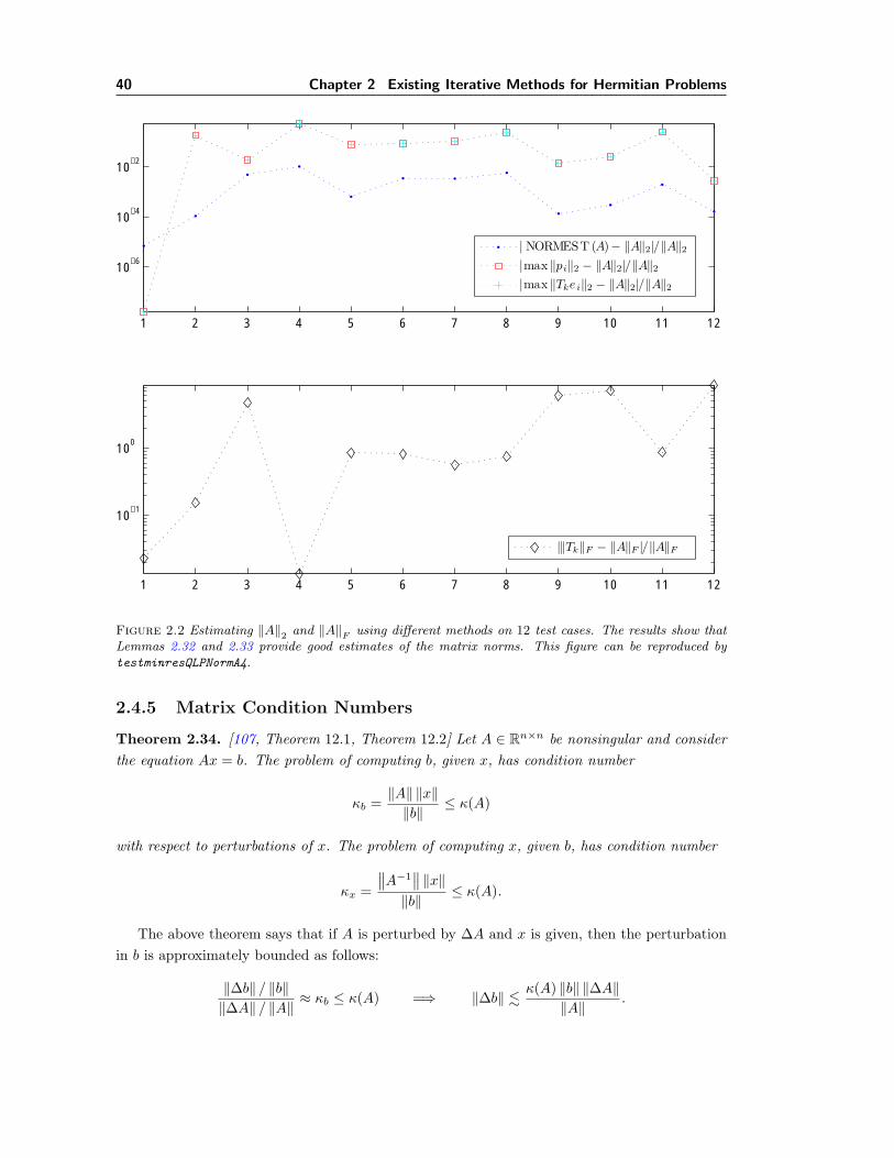
2.1 The loss of orthogonality in Lanczos implies convergence of solution in Ax = b. . 182.2 Estimating ‖A‖2 and ‖A‖F using different methods in MINRES. . . . . . . . . . 40
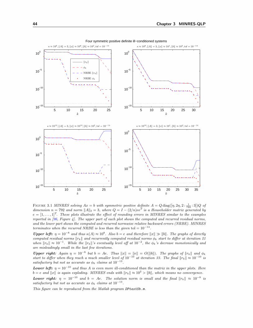
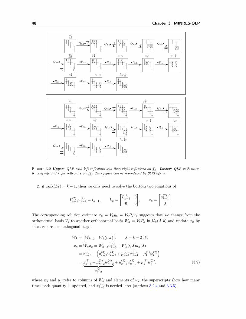
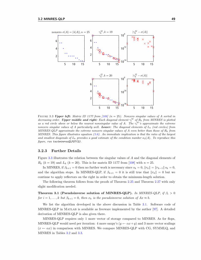
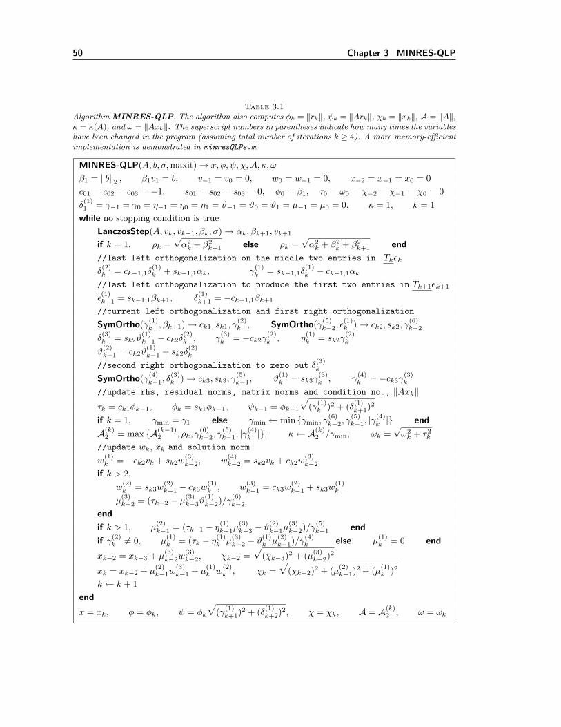
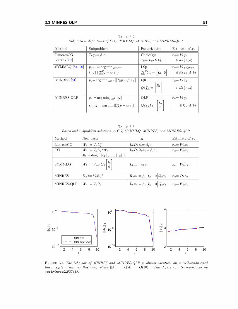
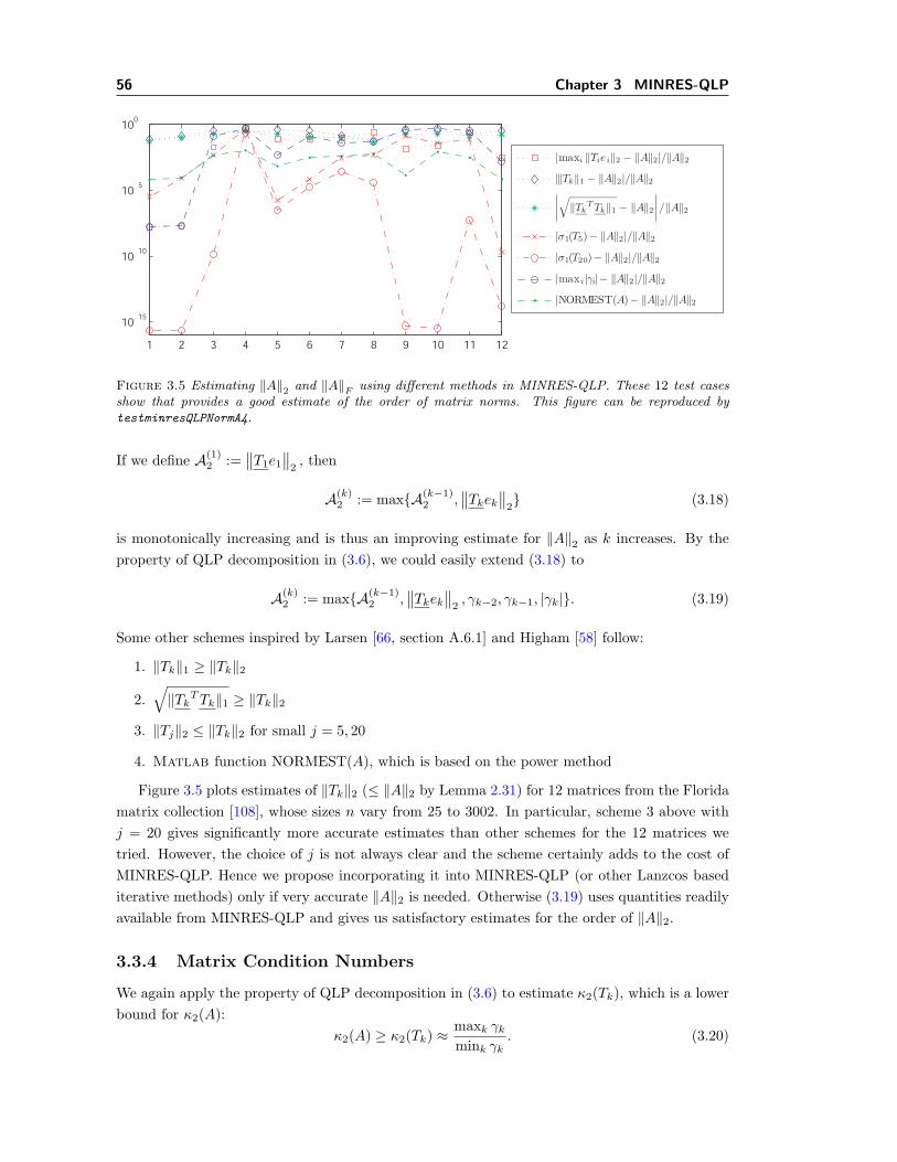
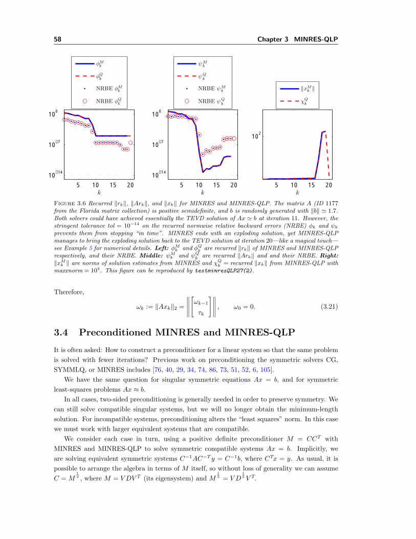
3.1 Rounding errors in MINRES on ill-conditioned systems. . . . . . . . . . . . . . . 443.2 MINRES-QLP with and without interleaving left and right reflectors. . . . . . . 483.3 The ratio of Lk’s extreme diagonal entries from MINRES-QLP approximates κ(A). 493.4 MINRES and MINRES-QLP on a well-conditioned linear system. . . . . . . . . . 513.5 Estimating ‖A‖2 using different methods in MINRES-QLP. . . . . . . . . . . . . 563.6 Norms of solution estimates from MINRES and MINRES-QLP min ‖Ax− b‖. . . 58
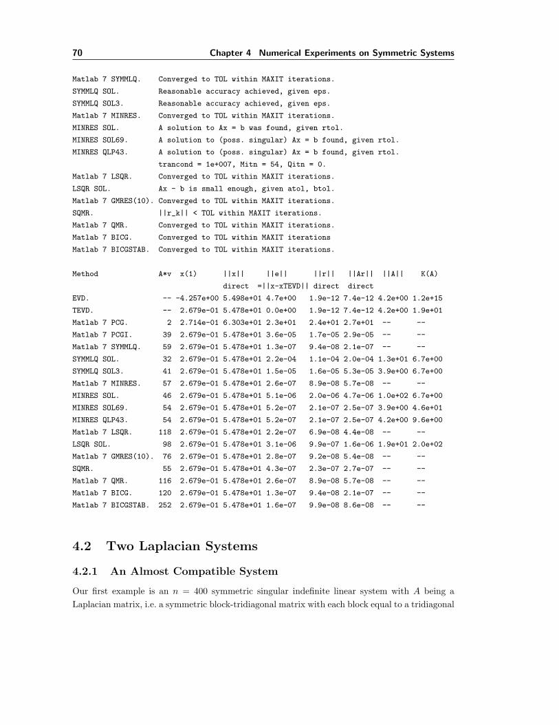
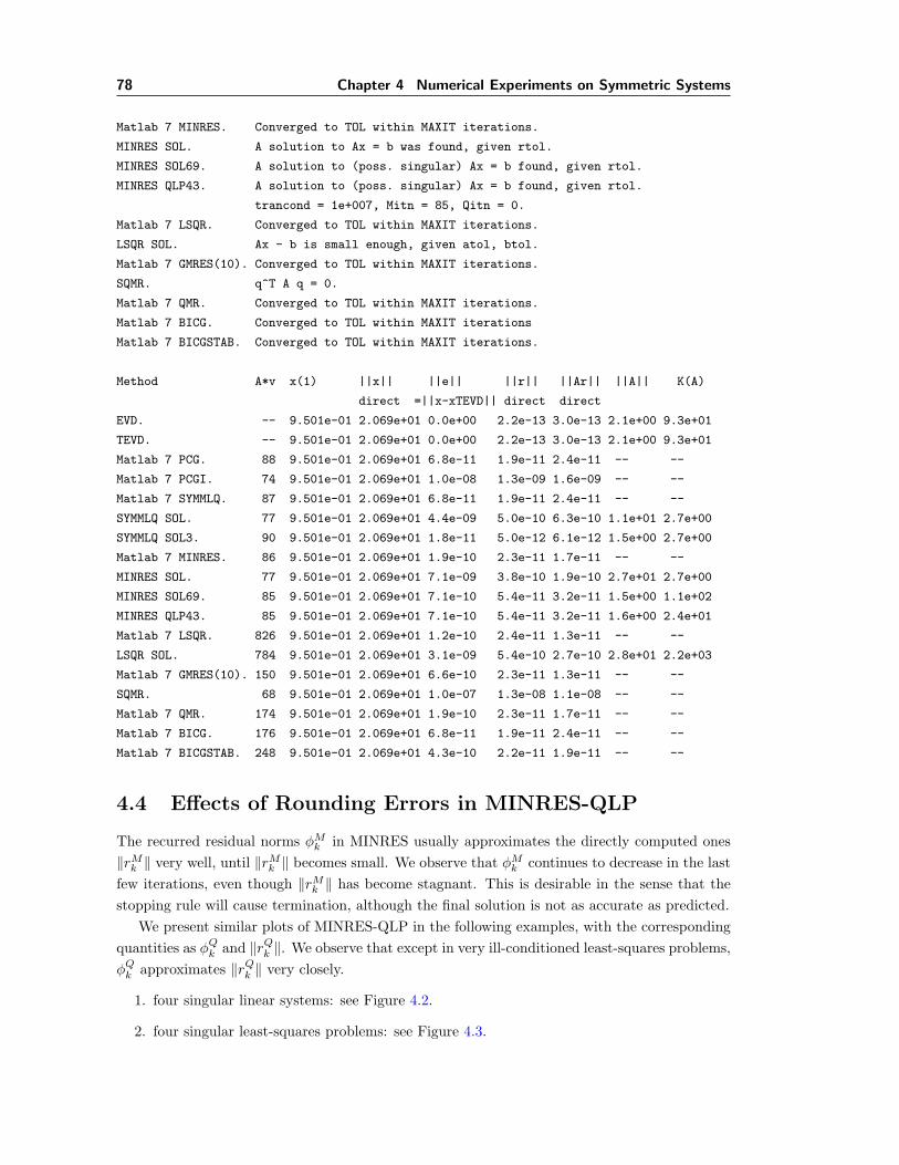
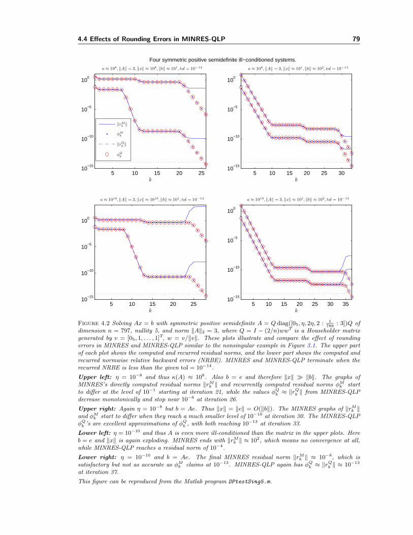
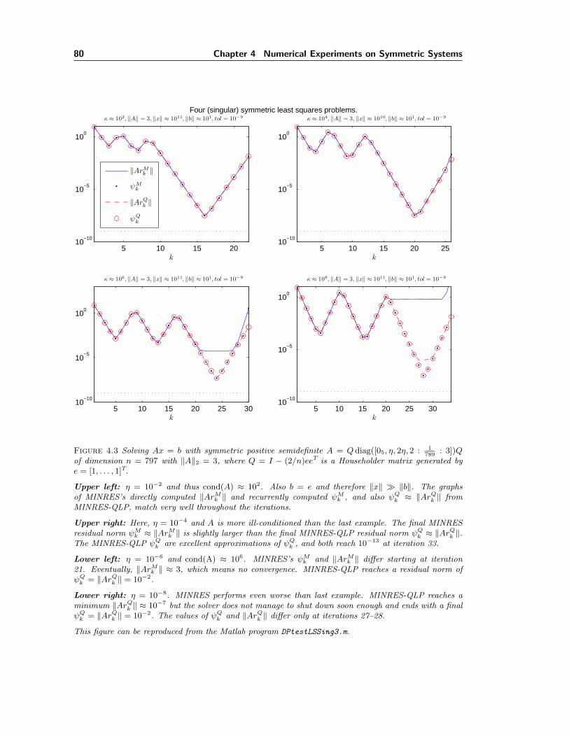
4.1 Example: Indefinite and singular Ax = b. . . . . . . . . . . . . . . . . . . . . . . 714.2 Rounding errors in MINRES-QLP (cf. MINRES) on ill-conditioned systems. . . . 794.3 Rounding errors in MINRES-QLP (cf. MINRES) on least-squares problems. . . . 80
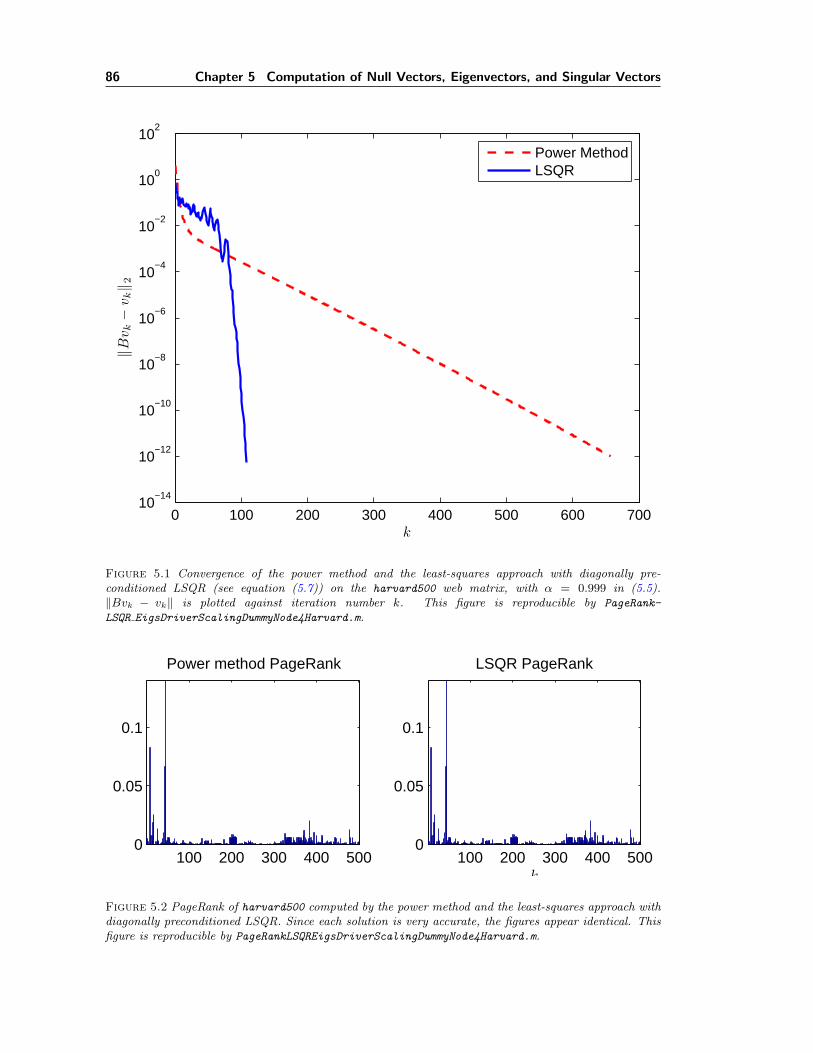
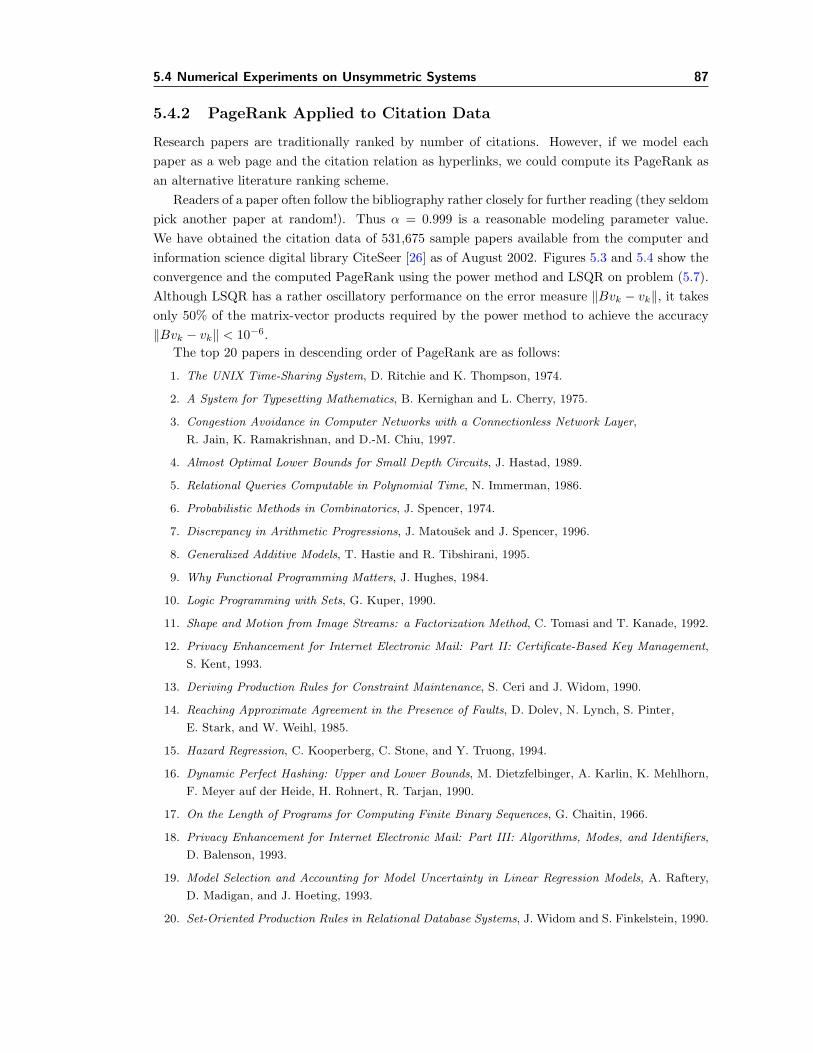
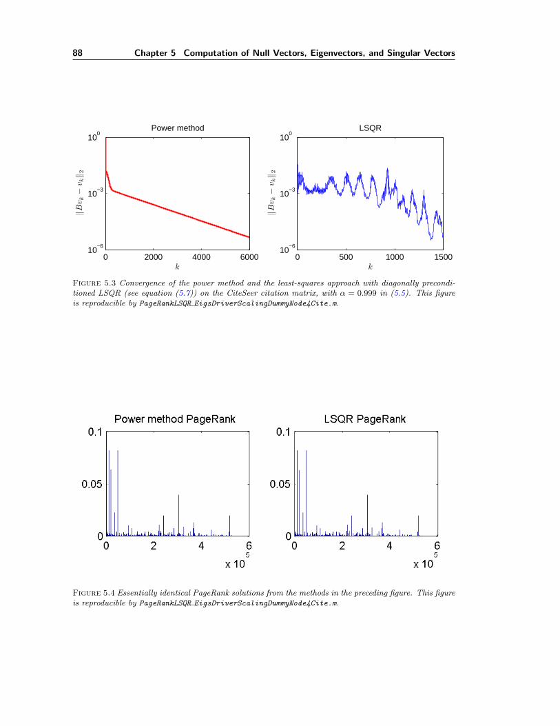
5.1 Convergence of the power method and LSQR on harvard500. . . . . . . . . . . . 865.2 PageRank of harvard500. . . . . . . . . . . . . . . . . . . . . . . . . . . . . . . . 865.3 Convergence of the power method and LSQR on CiteSeer data. . . . . . . . . . . 885.4 PageRank of CiteSeer data. . . . . . . . . . . . . . . . . . . . . . . . . . . . . . . 885.5 A multiple null-vector problem that arises from helioseismology. . . . . . . . . . . 89
xiv
Chapter 1
Introduction
1.1 The Motivating Problem
In 1998 when the Google PageRank algorithm was first described [16], the World Wide Webcontained about 150 million web pages and the classical power method appeared to be effectivefor computing the relevant matrix eigenvector. By 2003, the number of web pages had grown to 2billion, and the power method was still being used (monthly) to compute an up-to-date rankingvector. Given some initial eigenvector estimate v0, the power method involves the iteration
where A is a square matrix with rows and columns corresponding to web pages, and Aij 6= 0if there is a link from page j to page i. Each column of A sums to 1 and thus A is called acolumn-stochastic matrix. Moreover, if its underlying graph is strongly connected, then by thePerron-Frobenius theorem, A would have a simple dominant eigenvalue of 1 and thus the powermethod is applicable. In practice, the convergence of (1.1) appeared to be remarkably good. Therequired number of iterations kP was at most a few hundred.
Much analysis has since been done (e.g., [31, 64]), but at this stage, there was still room foroptimistic researchers [18, 42, 46] to believe that Krylov subspace methods might prove usefulin place of the power method. Since the related eigenvalue is known to be 1, the method ofinverse iteration [50, p. 362], [87] could be used. This involves a sequence of linear systems inthe following iteration:
(A− I)xk = vk−1, vk = xk/‖xk‖, k = 1, . . . , kI , (1.2)
where the number of iterations kI would be only 1 or 2. The matrix A−I is intentionally singular,and the computed solutions xk are expected to grow extremely large (‖xk‖ ≈ 1/ε, where ε isthe machine precision), so that the normalized vectors vk would satisfy (A− I)vk ≈ 0 and henceAvk ≈ vk as required.
Of course, Krylov subspace methods involve many matrix-vector products Av (as in the powermethod) and additional storage in the form of some very large work vectors.
1.1.1 Null Vectors
The Google matrix A is square but unsymmetric. With the PageRank computation in mind, wewere motivated to investigate the use of LSQR [82, 83] on singular least-squares systems
minx‖Ax− b‖2, A ∈ Rm×n, rank(A) < n (1.3)
1
2 Chapter 1 Introduction
in order to compute null vectors v satisfying Av ≈ 0. (We have now replaced A − I by A,and A may be rectangular.) For almost any nonzero vector b, the computed solution x shouldbe extremely large in norm, and the normalized vector v = x/‖x‖ will be a null vector of A.
Our first test matrix A was derived from AH , the 500 × 500 unsymmetric Harvard matrixcalled harvard500 assembled by Cleve Moler [71] to simulate the PageRank problem. Withnormal stopping tolerances in place, we found that LSQR converged to a least-squares solutionthat did not have large norm (and was not a null vector of A). Only after disabling all stoppingconditions were we able to force LSQR to continue iterating until the solution norm finallyincreased toward 1/ε, giving a null vector v = x/‖x‖ as required.
1.1.2 A Revelation
The question arose: Which solution x was LSQR converging to with the normal stopping ruleswhen A was singular? Probably it was the minimum-length solution in which ‖x‖2 is minimizedamong the (infinitely many) solutions that minimize ‖Ax − b‖2. In any case, the associatedresidual vector r = b − Ax was satisfying ATr = 0 because LSQR’s stopping rules require‖ATr‖/(‖A‖‖r‖) to be small when ‖r‖ 6= 0. Suddenly we realized that we were computing a nullvector for the transpose matrix AT. This implied that to obtain a null vector for the singularmatrix A in (1.3), we could solve the least-squares problem
miny‖ATy − c‖2, A ∈ Rm×n, rank(A) < n (1.4)
with some rather arbitrary vector c. The optimal residual s = c − ATy would satisfy As = 0,and the required null vector would be v = s/‖s‖. Furthermore, LSQR should converge sooneron (1.4) than if we force it to compute a very large x for (1.3).
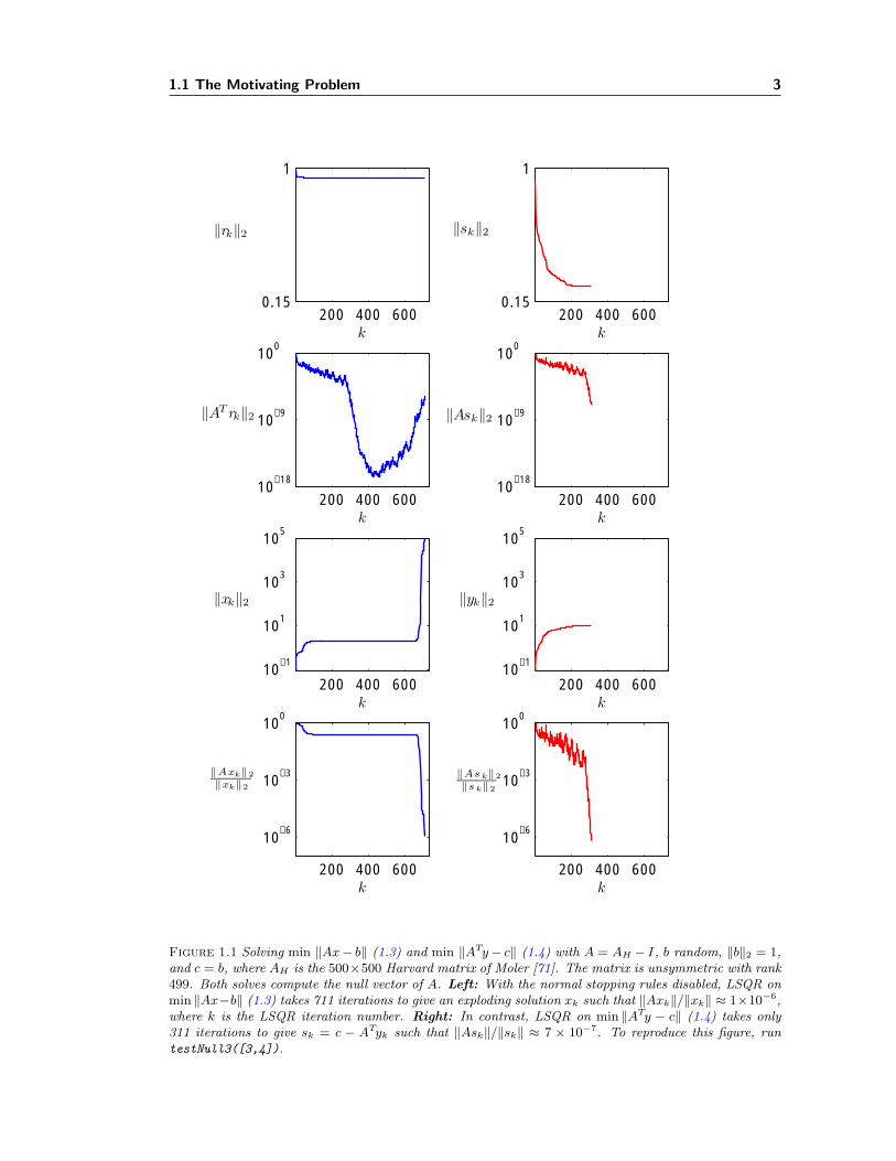
Figure 1.1 shows LSQR converging twice as quickly on (1.4) compared to (1.3).
1.1.3 Symmetric Systems
At some point another question arose: What would happen in the symmetric case? Both thesystems (1.3) and (1.4) take the form
minx‖Ax− b‖2, A ∈ Rn×n and symmetric, rank(A) < n. (1.5)
For general symmetric A (not necessarily positive definite), the natural Krylov subspace methodsare SYMMLQ and MINRES [81]. When A is singular, MINRES is the logical choice because itallows the residual r = b−Ax to be nonzero. In all cases, the optimal residual satisfies Ar = 0.If b happens to lie in the range of A, the optimal residual is r = 0, but otherwise—for example, ifb is a random vector—we can expect r 6= 0, so that v = r/‖r‖ will be a null vector, and again itwill be obtained sooner than if we force iterations to continue until ‖x‖ is extremely large. In aleast-squares problem, ‖r‖ > 0 and thus MINRES would need new stopping conditions to detectif ‖Ax‖/‖x‖ or ‖Ar‖/‖r‖ were small enough. We derive recurrence relations for ‖Ax‖ and ‖Ar‖that give us accurate estimates without extra matrix-vector multiplications.
We created our second test matrix from harvard500 by defining A = AH + ATH and con-structing a diagonal matrix D with diagonal elements d(i) = 1/
√‖A(i, :)‖1, which is well-defined
1.1 The Motivating Problem 3
200 400 6000.15
1
‖rk‖2
k
200 400 60010
−18
10−9
100
‖AT rk‖2
k
200 400 60010
−1
101
103
105
‖xk‖2
k
200 400 600
10−6
10−3
100
‖Axk‖2‖xk‖2
k
200 400 6000.15
1
‖sk‖2
k
200 400 60010
−18
10−9
100
‖Ask‖2
k
200 400 60010
−1
101
103
105
‖yk‖2
k
200 400 600
10−6
10−3
100
‖As k‖2‖s k‖2
k
Figure 1.1 Solving min ‖Ax− b‖ (1.3) and min ‖ATy− c‖ (1.4) with A = AH − I, b random, ‖b‖2 = 1,and c = b, where AH is the 500×500 Harvard matrix of Moler [71]. The matrix is unsymmetric with rank499. Both solves compute the null vector of A. Left: With the normal stopping rules disabled, LSQR onmin ‖Ax−b‖ (1.3) takes 711 iterations to give an exploding solution xk such that ‖Axk‖/‖xk‖ ≈ 1×10⁻⁶,where k is the LSQR iteration number. Right: In contrast, LSQR on min ‖ATy − c‖ (1.4) takes only311 iterations to give sk = c − ATyk such that ‖Ask‖/‖sk‖ ≈ 7 × 10⁻⁷. To reproduce this figure, runtestNull3([3,4]).
4 Chapter 1 Introduction
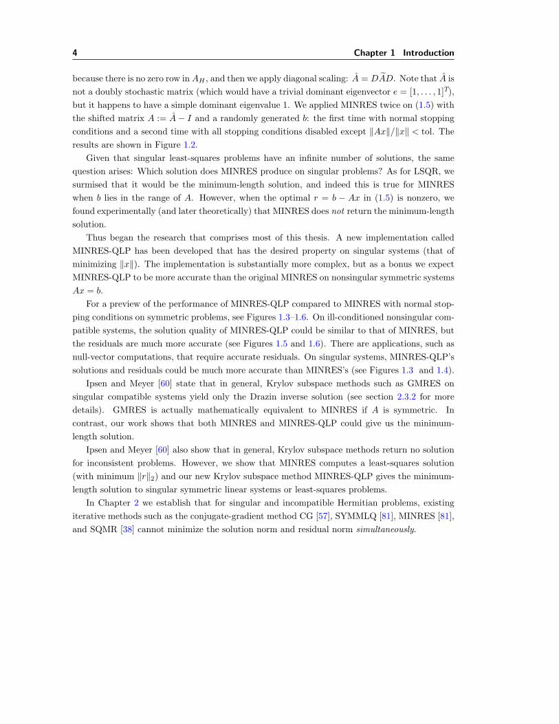
because there is no zero row in AH , and then we apply diagonal scaling: A = DAD. Note that A isnot a doubly stochastic matrix (which would have a trivial dominant eigenvector e = [1, . . . , 1]T),but it happens to have a simple dominant eigenvalue 1. We applied MINRES twice on (1.5) withthe shifted matrix A := A− I and a randomly generated b: the first time with normal stoppingconditions and a second time with all stopping conditions disabled except ‖Ax‖/‖x‖ < tol. Theresults are shown in Figure 1.2.
Given that singular least-squares problems have an infinite number of solutions, the samequestion arises: Which solution does MINRES produce on singular problems? As for LSQR, wesurmised that it would be the minimum-length solution, and indeed this is true for MINRESwhen b lies in the range of A. However, when the optimal r = b − Ax in (1.5) is nonzero, wefound experimentally (and later theoretically) that MINRES does not return the minimum-lengthsolution.
Thus began the research that comprises most of this thesis. A new implementation calledMINRES-QLP has been developed that has the desired property on singular systems (that ofminimizing ‖x‖). The implementation is substantially more complex, but as a bonus we expectMINRES-QLP to be more accurate than the original MINRES on nonsingular symmetric systemsAx = b.
For a preview of the performance of MINRES-QLP compared to MINRES with normal stop-ping conditions on symmetric problems, see Figures 1.3–1.6. On ill-conditioned nonsingular com-patible systems, the solution quality of MINRES-QLP could be similar to that of MINRES, butthe residuals are much more accurate (see Figures 1.5 and 1.6). There are applications, such asnull-vector computations, that require accurate residuals. On singular systems, MINRES-QLP’ssolutions and residuals could be much more accurate than MINRES’s (see Figures 1.3 and 1.4).
Ipsen and Meyer [60] state that in general, Krylov subspace methods such as GMRES onsingular compatible systems yield only the Drazin inverse solution (see section 2.3.2 for moredetails). GMRES is actually mathematically equivalent to MINRES if A is symmetric. Incontrast, our work shows that both MINRES and MINRES-QLP could give us the minimum-length solution.
Ipsen and Meyer [60] also show that in general, Krylov subspace methods return no solutionfor inconsistent problems. However, we show that MINRES computes a least-squares solution(with minimum ‖r‖2) and our new Krylov subspace method MINRES-QLP gives the minimum-length solution to singular symmetric linear systems or least-squares problems.
In Chapter 2 we establish that for singular and incompatible Hermitian problems, existingiterative methods such as the conjugate-gradient method CG [57], SYMMLQ [81], MINRES [81],and SQMR [38] cannot minimize the solution norm and residual norm simultaneously.
1.1 The Motivating Problem 5
20 40 60 800.75
0.8
0.85
‖rk‖2
k
20 40 60 8010
−9
10−6
10−3
100
‖Ark‖2
k
20 40 60 80
101
103
105
‖xk‖2
k
20 40 60 80
10−5
10−3
10−1
‖Axk‖2‖xk‖2
k
20 40 60 800.75
0.8
0.85
‖rk‖2
k
20 40 60 8010
−9
10−6
10−3
100
‖Ark‖2
k
20 40 60 80
101
103
105
‖xk‖2
k
20 40 60 80
10−5
10−3
10−1
‖Ark‖2‖rk‖2
k
Figure 1.2 Solving min ‖Ax− b‖ (1.5) with A := A− I, where A is a symmetrized and scaled form ofthe 500 × 500 Harvard matrix AH (see text in section 1.1.3), b random, and ‖b‖2 = 1. The matrix hasrank 499. Left: With all stopping rules disabled except ‖Axk‖/‖xk‖ < tol = 10−5, MINRES takes 77iterations to give an exploding solution xk such that ‖xk‖ ≈ 8× 10⁴ and ‖Axk‖/‖xk‖ ≈ 7× 10⁻⁶.Right: In contrast, MINRES with normal stopping conditions takes only about 42 iterations to give rk
such that ‖rk‖ ≈ 0.78 and ‖Ark‖/‖rk‖ ≈ 1 × 10⁻⁵. Since the system is incompatible, MINRES needsnew stopping conditions to detect if ‖Axk‖/‖xk‖ or ‖Ark‖ is small enough. To reproduce this figure, runtestNull3([5,6]).
6 Chapter 1 Introduction
20 40 60 800.75
0.8
0.85
‖rk‖2
k20 40 60 80
10−9
10−6
10−3
100
‖Ark‖2
k20 40 60 80
101
103
105
‖xk‖2
k
MINRES
MINRES−QLP
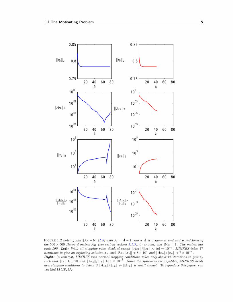
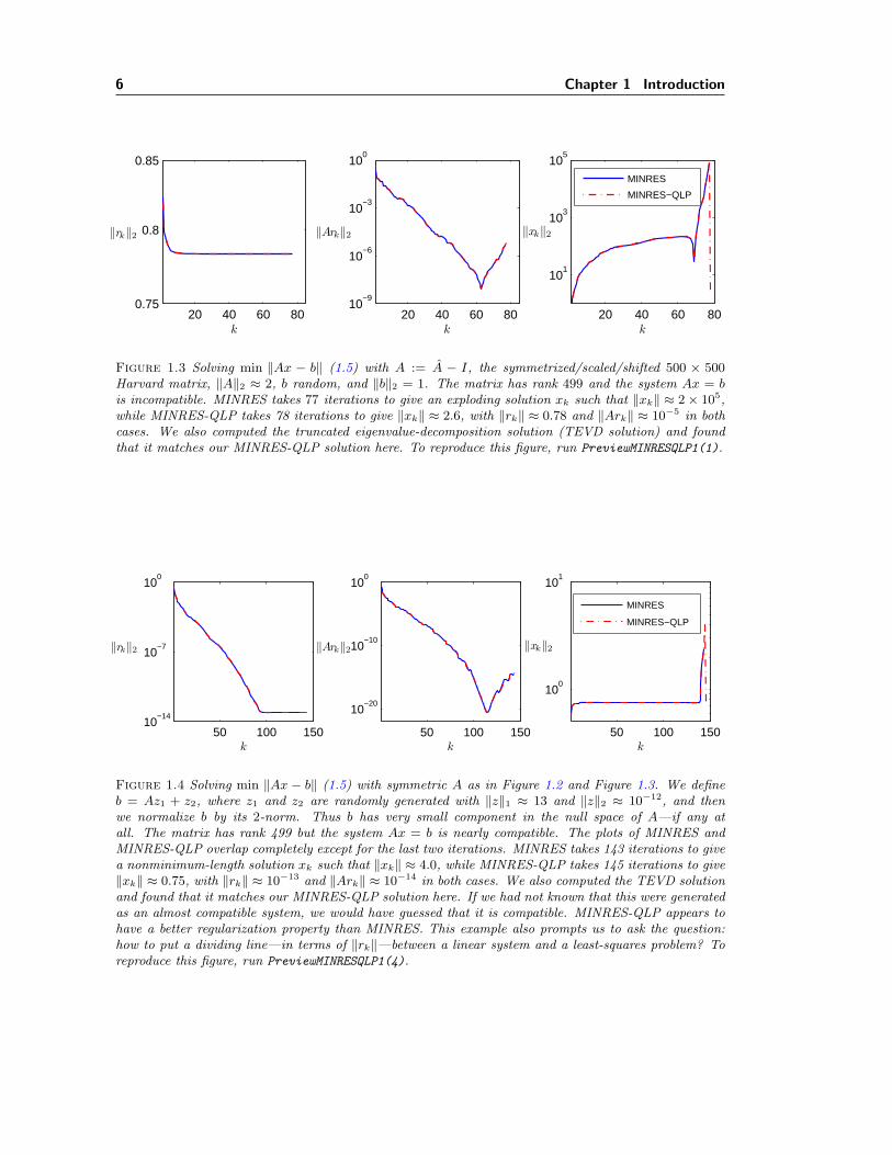
Figure 1.3 Solving min ‖Ax − b‖ (1.5) with A := A − I, the symmetrized/scaled/shifted 500 × 500Harvard matrix, ‖A‖2 ≈ 2, b random, and ‖b‖2 = 1. The matrix has rank 499 and the system Ax = bis incompatible. MINRES takes 77 iterations to give an exploding solution xk such that ‖xk‖ ≈ 2× 10⁵,while MINRES-QLP takes 78 iterations to give ‖xk‖ ≈ 2.6, with ‖rk‖ ≈ 0.78 and ‖Ark‖ ≈ 10−5 in bothcases. We also computed the truncated eigenvalue-decomposition solution (TEVD solution) and foundthat it matches our MINRES-QLP solution here. To reproduce this figure, run PreviewMINRESQLP1(1).
50 100 15010
−14
10−7
100
‖rk‖2
k50 100 150
10−20
10−10
100
‖Ark‖2
k50 100 150
100
101
‖xk‖2
k
MINRES
MINRES−QLP
Figure 1.4 Solving min ‖Ax − b‖ (1.5) with symmetric A as in Figure 1.2 and Figure 1.3. We defineb = Az1 + z2, where z1 and z2 are randomly generated with ‖z‖1 ≈ 13 and ‖z‖2 ≈ 10−12, and thenwe normalize b by its 2-norm. Thus b has very small component in the null space of A—if any atall. The matrix has rank 499 but the system Ax = b is nearly compatible. The plots of MINRES andMINRES-QLP overlap completely except for the last two iterations. MINRES takes 143 iterations to givea nonminimum-length solution xk such that ‖xk‖ ≈ 4.0, while MINRES-QLP takes 145 iterations to give‖xk‖ ≈ 0.75, with ‖rk‖ ≈ 10−13 and ‖Ark‖ ≈ 10−14 in both cases. We also computed the TEVD solutionand found that it matches our MINRES-QLP solution here. If we had not known that this were generatedas an almost compatible system, we would have guessed that it is compatible. MINRES-QLP appears tohave a better regularization property than MINRES. This example also prompts us to ask the question:how to put a dividing line—in terms of ‖rk‖—between a linear system and a least-squares problem? Toreproduce this figure, run PreviewMINRESQLP1(4).
1.1 The Motivating Problem 7
10 20 3027
28
29
‖xk‖2
k10 20 30
10−12
10−8
10−4
100
k
‖rk‖2
10 20 3010
−14
10−7
100
‖Ark‖2
k
MINRES
MINRES−QLP
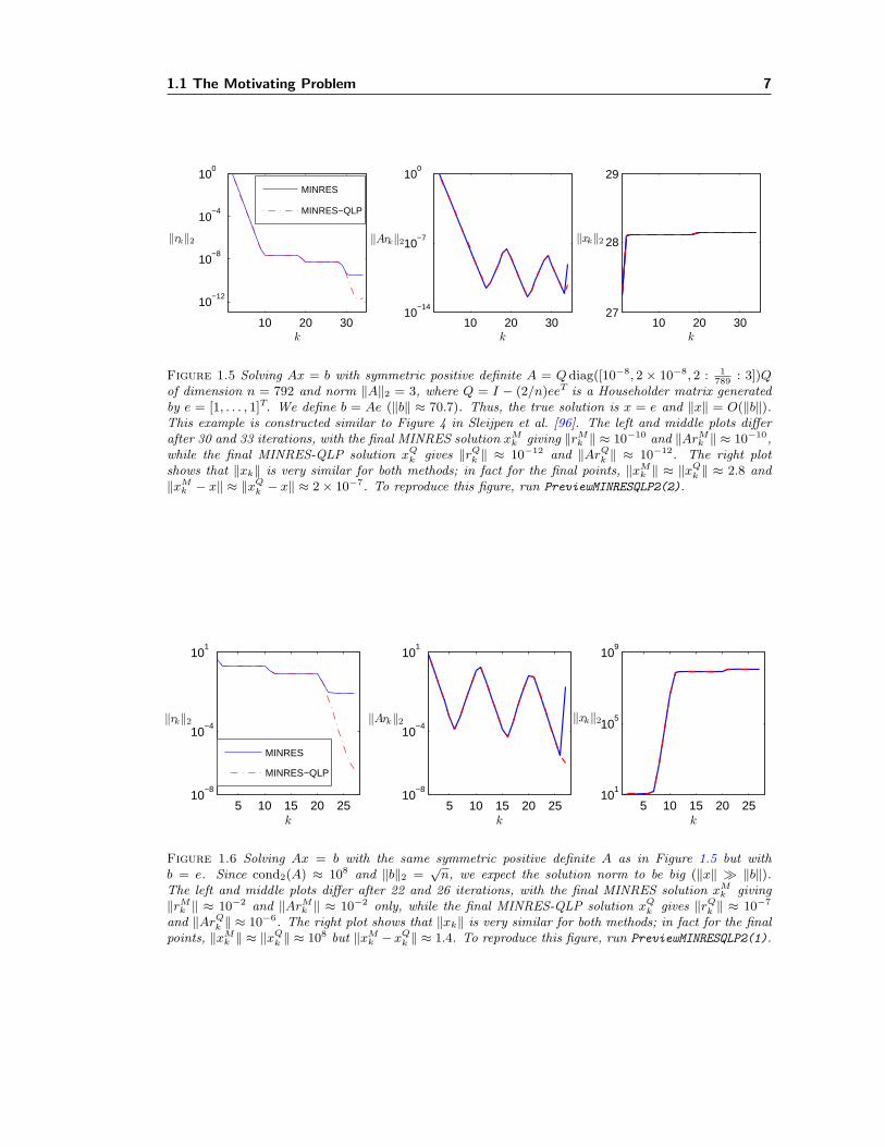
Figure 1.5 Solving Ax = b with symmetric positive definite A = Qdiag([10−8, 2 × 10⁻⁸, 2 : 1789
: 3])Qof dimension n = 792 and norm ‖A‖2 = 3, where Q = I − (2/n)eeT is a Householder matrix generatedby e = [1, . . . , 1]T. We define b = Ae (‖b‖ ≈ 70.7). Thus, the true solution is x = e and ‖x‖ = O(‖b‖).This example is constructed similar to Figure 4 in Sleijpen et al. [96]. The left and middle plots differafter 30 and 33 iterations, with the final MINRES solution xM
k giving ‖rMk ‖ ≈ 10−10 and ‖ArM
k ‖ ≈ 10−10,while the final MINRES-QLP solution xQ
k gives ‖rQk ‖ ≈ 10−12 and ‖ArQ
k ‖ ≈ 10−12. The right plotshows that ‖xk‖ is very similar for both methods; in fact for the final points, ‖xM
k ‖ ≈ ‖xQk ‖ ≈ 2.8 and
‖xMk − x‖ ≈ ‖xQ
k − x‖ ≈ 2× 10⁻⁷. To reproduce this figure, run PreviewMINRESQLP2(2).
5 10 15 20 2510
−8
10−4
101
k
‖rk‖2
5 10 15 20 2510
−8
10−4
101
‖Ark‖2
k5 10 15 20 25
101
105
109
‖xk‖2
k
MINRES
MINRES−QLP
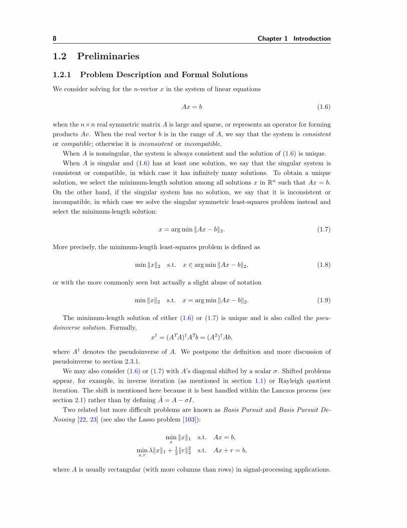
Figure 1.6 Solving Ax = b with the same symmetric positive definite A as in Figure 1.5 but withb = e. Since cond2(A) ≈ 108 and ‖b‖2 =
√n, we expect the solution norm to be big (‖x‖ � ‖b‖).
The left and middle plots differ after 22 and 26 iterations, with the final MINRES solution xMk giving
‖rMk ‖ ≈ 10−2 and ‖ArM
k ‖ ≈ 10−2 only, while the final MINRES-QLP solution xQk gives ‖rQ
k ‖ ≈ 10−7
and ‖ArQk ‖ ≈ 10−6. The right plot shows that ‖xk‖ is very similar for both methods; in fact for the final
points, ‖xMk ‖ ≈ ‖xQ
k ‖ ≈ 108 but ‖xMk −xQ
k ‖ ≈ 1.4. To reproduce this figure, run PreviewMINRESQLP2(1).
8 Chapter 1 Introduction
1.2 Preliminaries
1.2.1 Problem Description and Formal Solutions
We consider solving for the n-vector x in the system of linear equations
Ax = b (1.6)
when the n×n real symmetric matrix A is large and sparse, or represents an operator for formingproducts Av. When the real vector b is in the range of A, we say that the system is consistentor compatible; otherwise it is inconsistent or incompatible.
When A is nonsingular, the system is always consistent and the solution of (1.6) is unique.When A is singular and (1.6) has at least one solution, we say that the singular system is
consistent or compatible, in which case it has infinitely many solutions. To obtain a uniquesolution, we select the minimum-length solution among all solutions x in Rn such that Ax = b.On the other hand, if the singular system has no solution, we say that it is inconsistent orincompatible, in which case we solve the singular symmetric least-squares problem instead andselect the minimum-length solution:
x = arg min ‖Ax− b‖2. (1.7)
More precisely, the minimum-length least-squares problem is defined as
min ‖x‖2 s.t. x ∈ arg min ‖Ax− b‖2, (1.8)
or with the more commonly seen but actually a slight abuse of notation
min ‖x‖2 s.t. x = arg min ‖Ax− b‖2. (1.9)
The minimum-length solution of either (1.6) or (1.7) is unique and is also called the pseu-doinverse solution. Formally,
x† = (ATA)†ATb = (A2)†Ab,
where A† denotes the pseudoinverse of A. We postpone the definition and more discussion ofpseudoinverse to section 2.3.1.
We may also consider (1.6) or (1.7) with A’s diagonal shifted by a scalar σ. Shifted problemsappear, for example, in inverse iteration (as mentioned in section 1.1) or Rayleigh quotientiteration. The shift is mentioned here because it is best handled within the Lanczos process (seesection 2.1) rather than by defining A = A− σI.
Two related but more difficult problems are known as Basis Pursuit and Basis Pursuit De-Noising [22, 23] (see also the Lasso problem [103]):
minx‖x‖1 s.t. Ax = b,
minx,r
λ‖x‖1 + 12‖r‖
22 s.t. Ax+ r = b,
where A is usually rectangular (with more columns than rows) in signal-processing applications.
1.2 Preliminaries 9
Table 1.1Existing iterative algorithms since CG was created in 1952. All methods require products Avk for asequence of vectors {vk}. The last column indicates whether a method also requires ATuk for a sequenceof vectors {uk}.
Linear Equations Authors Properties of A AT ?
CG Hestenes and Stiefel (1952) [57] Symmetric positive definite
CRAIG Faddeev and Faddeeva (1963)[33] Square or rectangular yesMINRES Paige and Saunders (1975) [81] Symmetric indefinite
SYMMLQ Paige and Saunders (1975) [81] Symmetric indefinite
Bi-CG Fletcher (1976)[35] Square unsymmetric yesLSQR Paige and Saunders (1982) [82, 83] Square or rectangular yesGMRES Saad and Schultz (1986) [89] Square unsymmetric
CGS Sonneveld (1989) [98] Square unsymmetric
QMR Freund and Nachtigal (1991) [37] Square unsymmetric yesBi-CGSTAB Van der Vorst (1992) [109] Square unsymmetric yesTFQMR Freund (1993) [36] Square unsymmetric
SQMR Freund and Nachtigal (1994) [38] Symmetric
Least Squares Authors Properties of A AT ?
CGLS Hestenes and Stiefel (1952) [57] Square or rectangular yesRRLS Chen (1975) [24] Square or rectangular yesRRLSQR Paige and Saunders (1982) [82] Square or rectangular yesLSQR Paige and Saunders (1982) [82] Square or rectangular yes
1.2.2 Existing Numerical Algorithms
In this thesis, we are interested in sparse matrices that are so large that direct factorizationmethods such as Gaussian elimination or Cholesky decomposition are not immediately applicable.Instead, iterative methods and in particular Krylov subspace methods are usually the methods ofchoice. For example, CG is designed for a symmetric positive definite matrix A (whose eigenvaluesare all positive), while SYMMLQ and MINRES are for an indefinite and symmetric matrix A
(whose eigenvalues could be positive, negative, or zero).The main existing iterative methods for symmetric and unsymmetric A are listed in Table 1.1.
1.2.3 Background for MINRES
MINRES, first proposed in [81, section 6], is an algorithm for solving indefinite symmetric linearsystems. A number of acceleration methods for MINRES using (block) preconditioners have beenproposed in [73, 51, 105]. Researchers in various science and engineering disciplines have foundMINRES useful in a range of applications, including:
• interior eigenvalue problems [72, 114]
• augmented systems [34]
• nonlinear eigenvalue problems [20]
10 Chapter 1 Introduction
• characterization of null spaces [21]
• symmetric generalized eigenvalue problems [74]
• singular value computations [112]
• semidefinite programming [111]
• generalized least-squares problems [115].
1.2.4 Notation
We keep the lower-case letters i, j, k as subscripts to denote integer indices, c and s to denotecosine and sine of some angle θ, n for order of matrices and length of vectors, and other lower-caseletters such as b, u, v, w and x (possibly with integer subscripts) to denote column vectors oflength n. In particular, ek denotes the kth unit vector. We use upper-case italic letters (possiblywith integer subscripts) to denote matrices. The exception is superscript T , which denotes thetranspose of a vector or matrix. We reserve Ik to denote identity matrix of order k, and Qk andPk for orthogonal matrices. Lower-case Greek letters denote scalars. The symbol ‖·‖ denotesthe 2-norm of a vector or the Frobenius norm of a matrix. We use κ(A) to denote the conditionnumber of matrix A; R(A) and N (A) to denote the range and null space of A; Kk(A, b) to denotethe kth Krylov subspace of A and b; and A† is the pseudoinverse of A. We use A � 0 to denotethat A is positive definite, A � 0 to mean that A is not positive definite (so A could be negativedefinite, non-negative definite, indefinite, and so on). When we have a compatible linear system,we often write Ax = b. If the linear system is incompatible, we write Ax ≈ b as shorthand for thecorresponding linear least-squares problem min ‖Ax− b‖2. We use symbols ‖ to denote parallelvectors, and ⊥ to denote orthogonality.
Most of the results in our discussion are directly extendable to problems with complex matricesand vectors. When special care is needed in handling complex problems, we will be very specific.We use superscript H to denote the conjugate transpose of a complex matrix or vector.
1.2.5 Computations
We use Matlab 7.0 and double precision for computations unless otherwise specified. Weuse ε (varepsilon) to denote machine precision (= 2−52 ≈ 2.2 × 10⁻¹⁶). In an algorithm, weuse // to indicate comments. For measuring mathematical quantities or complexity of algorithms,sometimes we use big-oh O(·) to denote an asymptotic upper bound [94, Definition 7.2]:
f(n) = O(g(n)) if ∃ c > 0 and a positive integer n0 ∈ N such that ∀n ∈ N, n ≥ n0,f(n) ≤ cg(n).
Thus a nonzero constant α = O(1) = O(n) and αn = O(n). We note that f(n) = O(g(n)) is aslight abuse of notation—to be precise, it is f(n) ∈ O(g(n)).
Following the philosophy of reproducible computational research as advocated in [27, 25], foreach figure and example we mention either the source or the specific Matlab command.
1.2 Preliminaries 11
1.2.6 Roadmap
We review the iterative algorithms CG, SYMMLQ, and MINRES for Hermitian linear systemsand least-squares problems in Chapter 2, and show that MINRES gives a nonminimum-lengthsolution for inconsistent systems. We also review other Krylov subspace methods such as LSQRand GMRES for non-Hermitian problems, and we derive new recursive formulas for efficientestimation of ‖Ark‖, ‖Axk‖, and the condition number of A for MINRES.
In Chapter 3, we present a new algorithm MINRES-QLP for symmetric and possibly singularsystems. Chapter 4 gives numerical examples that contrast the solutions of MINRES with theminimum-length solutions of MINRES-QLP on symmetric and Hermitian systems.
In Chapter 5, we return to the null-vector problem for sparse matrices or linear operators,and apply the previously mentioned iterative solvers.
Chapter 6 summarizes our contributions and ongoing work.
12
Chapter 2
Existing Iterative Methods for
Hermitian Problems
In this chapter, we review the Lanczos process and the three best known algorithms for Hermi-tian linear systems: CG, SYMMLQ, and MINRES. In particular, we emphasize the recurrencerelations of various mathematical objects. We assume throughout that A ∈ Rn×n, b ∈ Rn, A 6= 0,and b 6= 0. However, the algorithms are readily extended to Hermitian A and complex b.
2.1 The Lanczos Process
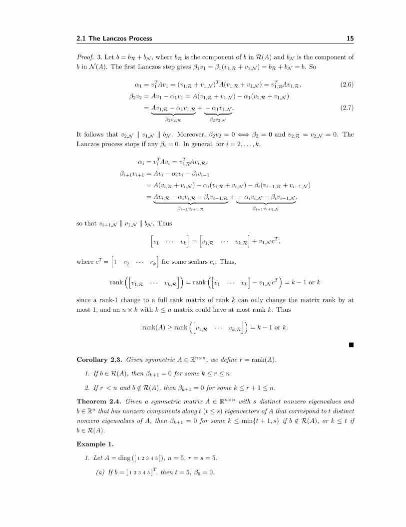
The Lanczos process transforms a symmetric matrix A to a symmetric tridiagonal matrix withan additional row at the bottom:
Tk =
α1 β2
β2 α2 β3
β3 α3. . .
. . . . . . βk
βk αk
βk+1
.
If we define Tk to be the first k rows of Tk, then Tk is square and symmetric, and
Tk =
[Tk
βk+1eTk
], Tk =
[Tk−1 βkek−1
βkeTk−1 αk
].
The Lanczos process iteratively computes vectors vk as follows:
v0 = 0, β1v1 = b, where β1 serves to normalize v1, (2.1)
pk = Avk, αk = vTkpk,
βk+1vk+1 = pk − αkvk − βkvk−1, where βk+1 serves to normalize vk+1. (2.2)
In matrix form,AVk = Vk+1Tk, where Vk =
[v1 · · · vk
]. (2.3)
In exact arithmetic, the columns of Vk are orthonormal and the process stops when βk+1 = 0(k ≤ n), and then we obtain
AVk = VkTk. (2.4)
13
14 Chapter 2 Existing Iterative Methods for Hermitian Problems
Tridiag(A, b, σ,maxit)→ Tk, Vk //partial tridiagonalization of A− σIβ1 = ‖b‖2, v0 = 0, β1 = ‖b‖, k = 1if β1 6= 0, v1 = b/β1 end
while βk 6= 0 and k ≤ maxitLanczosStep(A, vk, vk−1, βk, σ)→ αk, βk+1, vk+1
k ← k + 1end
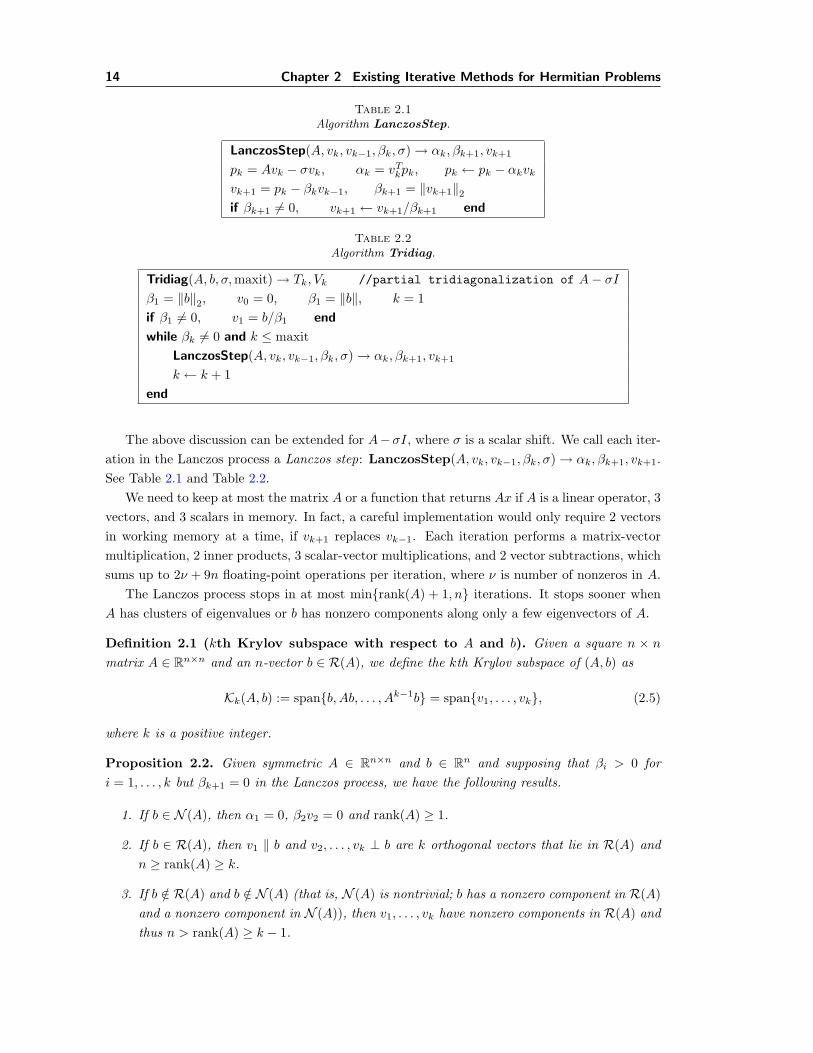
The above discussion can be extended for A−σI, where σ is a scalar shift. We call each iter-ation in the Lanczos process a Lanczos step: LanczosStep(A, vk, vk−1, βk, σ)→ αk, βk+1, vk+1.See Table 2.1 and Table 2.2.
We need to keep at most the matrix A or a function that returns Ax if A is a linear operator, 3vectors, and 3 scalars in memory. In fact, a careful implementation would only require 2 vectorsin working memory at a time, if vk+1 replaces vk−1. Each iteration performs a matrix-vectormultiplication, 2 inner products, 3 scalar-vector multiplications, and 2 vector subtractions, whichsums up to 2ν + 9n floating-point operations per iteration, where ν is number of nonzeros in A.
The Lanczos process stops in at most min{rank(A) + 1, n} iterations. It stops sooner whenA has clusters of eigenvalues or b has nonzero components along only a few eigenvectors of A.
Definition 2.1 (kth Krylov subspace with respect to A and b). Given a square n × nmatrix A ∈ Rn×n and an n-vector b ∈ R(A), we define the kth Krylov subspace of (A, b) as
Proposition 2.2. Given symmetric A ∈ Rn×n and b ∈ Rn and supposing that βi > 0 fori = 1, . . . , k but βk+1 = 0 in the Lanczos process, we have the following results.
1. If b ∈ N (A), then α1 = 0, β2v2 = 0 and rank(A) ≥ 1.
2. If b ∈ R(A), then v1 ‖ b and v2, . . . , vk ⊥ b are k orthogonal vectors that lie in R(A) andn ≥ rank(A) ≥ k.
3. If b /∈ R(A) and b /∈ N (A) (that is, N (A) is nontrivial; b has a nonzero component in R(A)and a nonzero component in N (A)), then v1, . . . , vk have nonzero components in R(A) andthus n > rank(A) ≥ k − 1.
2.1 The Lanczos Process 15
Proof. 3. Let b = bR + bN , where bR is the component of b in R(A) and bN is the component ofb in N (A). The first Lanczos step gives β1v1 = β1(v1,R + v1,N ) = bR + bN = b. So
It follows that v2,N ‖ v1,N ‖ bN . Moreover, β2v2 = 0 ⇐⇒ β2 = 0 and v2,R = v2,N = 0. TheLanczos process stops if any βi = 0. In general, for i = 2, . . . , k,
since a rank-1 change to a full rank matrix of rank k can only change the matrix rank by atmost 1, and an n× k with k ≤ n matrix could have at most rank k. Thus
rank(A) ≥ rank([v1,R · · · vk,R
])= k − 1 or k.
�
Corollary 2.3. Given symmetric A ∈ Rn×n, we define r = rank(A).
1. If b ∈ R(A), then βk+1 = 0 for some k ≤ r ≤ n.
2. If r < n and b /∈ R(A), then βk+1 = 0 for some k ≤ r + 1 ≤ n.
Theorem 2.4. Given a symmetric matrix A ∈ Rn×n with s distinct nonzero eigenvalues andb ∈ Rn that has nonzero components along t (t ≤ s) eigenvectors of A that correspond to t distinctnonzero eigenvalues of A, then βk+1 = 0 for some k ≤ min{t + 1, s} if b /∈ R(A), or k ≤ t ifb ∈ R(A).
Example 1.
1. Let A = diag ([ 1 2 3 4 5 ]), n = 5, r = s = 5.
(a) If b = [ 1 2 3 4 5 ]T, then t = 5, β6 = 0.
16 Chapter 2 Existing Iterative Methods for Hermitian Problems
(b) If b = [ 1 2 0 0 0 ]T, then t = 2, β3 = 0.
2. Let A = diag ([ 1 2 3 0 0 ]), n = 5, r = s = 3.
(a) If b = [ 1 2 0 0 0 ]T, then b ∈ R(A), t = 2, β3 = 0.
(b) If b = [ 1 0 0 0 0 ]T, then b ∈ R(A), t = 1, β2 = 0.
(c) If b = [ 1 2 3 4 0 ]T, then b /∈ R(A), t = 3, β4 = 0.
(d) If b = [ 1 0 0 4 0 ]T, then b /∈ R(A), t = 1, β3 = 0.
3. Let A = diag ([ 2 2 3 0 0 ]) , r = 3, s = 2.
(a) If b = [ 1 2 0 0 0 ]T, then b ∈ R(A), t = 1, β3 = 0.
(b) If b = [ 1 2 3 4 0 ]T, then b /∈ R(A), t = 2, β4 = 0.
(c) If b = [ 1 0 0 4 0 ]T, then b /∈ R(A), t = 1, β3 = 0.
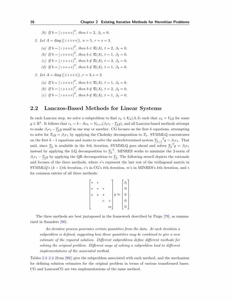
2.2 Lanczos-Based Methods for Linear Systems
In each Lanczos step, we solve a subproblem to find xk ∈ Kk(A, b) such that xk = Vky for somey ∈ Rk. It follows that rk = b−Axk = Vk+1(β1e1−Tky), and all Lanczos-based methods attemptto make β1e1−Tky small in one way or another. CG focuses on the first k equations, attemptingto solve for Tky = β1e1 by applying the Cholesky decomposition to Tk. SYMMLQ concentrateson the first k−1 equations and wants to solve the underdetermined system Tk−1
Ty = β1e1. Thatsaid, since Tk is available in the kth iteration, SYMMLQ goes ahead and solves TkTy = β1e1
instead by applying the LQ decomposition to TkT. MINRES works to minimize the 2-norm ofβ1e1 − Tky by applying the QR decomposition to Tk. The following stencil depicts the rationaleand focuses of the three methods, where s’s represent the last row of the tridiagonal matrix inSYMMLQ’s (k− 1)th iteration, c’s in CG’s kth iteration, m’s in MINRES’s kth iteration, and ∗for common entries of all three methods:
∗ ∗∗ ∗ ∗s s s
c c
m
y ≈
β1
0
0
0
0
.
The three methods are best juxtaposed in the framework described by Paige [79], as summa-rized in Saunders [90]:
An iterative process generates certain quantities from the data. At each iteration asubproblem is defined, suggesting how those quantities may be combined to give a newestimate of the required solution. Different subproblems define different methods forsolving the original problem. Different ways of solving a subproblem lead to differentimplementations of the associated method.
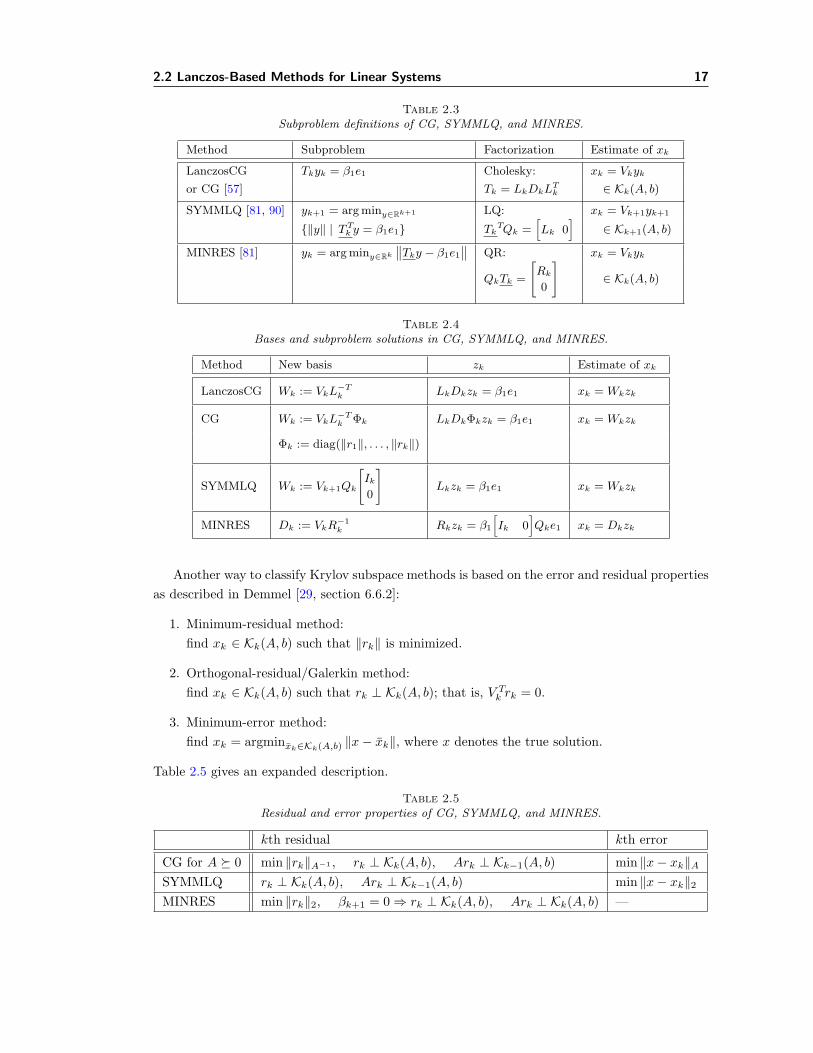
Tables 2.3–2.4 (from [90]) give the subproblem associated with each method, and the mechanismfor defining solution estimates for the original problem in terms of various transformed bases.CG and LanczosCG are two implementations of the same method.
2.2 Lanczos-Based Methods for Linear Systems 17
Table 2.3Subproblem definitions of CG, SYMMLQ, and MINRES.
Table 2.4Bases and subproblem solutions in CG, SYMMLQ, and MINRES.
Method New basis zk Estimate of xk
LanczosCG Wk := VkL−Tk LkDkzk = β1e1 xk = Wkzk
CG Wk := VkL−Tk Φk LkDkΦkzk = β1e1 xk = Wkzk
Φk := diag(‖r1‖, . . . , ‖rk‖)
SYMMLQ Wk := Vk+1Qk
[Ik
0
]Lkzk = β1e1 xk = Wkzk
MINRES Dk := VkR−1k Rkzk = β1
[Ik 0
]Qke1 xk = Dkzk
Another way to classify Krylov subspace methods is based on the error and residual propertiesas described in Demmel [29, section 6.6.2]:
1. Minimum-residual method:find xk ∈ Kk(A, b) such that ‖rk‖ is minimized.
2. Orthogonal-residual/Galerkin method:find xk ∈ Kk(A, b) such that rk ⊥ Kk(A, b); that is, V Tk rk = 0.
3. Minimum-error method:find xk = argminxk∈Kk(A,b) ‖x− xk‖, where x denotes the true solution.
Table 2.5 gives an expanded description.
Table 2.5Residual and error properties of CG, SYMMLQ, and MINRES.
kth residual kth error
CG for A � 0 min ‖rk‖A−1 , rk ⊥ Kk(A, b), Ark ⊥ Kk−1(A, b) min ‖x− xk‖ASYMMLQ rk ⊥ Kk(A, b), Ark ⊥ Kk−1(A, b) min ‖x− xk‖2MINRES min ‖rk‖2, βk+1 = 0⇒ rk ⊥ Kk(A, b), Ark ⊥ Kk(A, b) —
18 Chapter 2 Existing Iterative Methods for Hermitian Problems
20 40 60 80
10−15
10−10
10−5
|| VkT V
k − I ||∞
Iteration k Iteration k
localglobal
CSPY( | VkT V
k − I |)
0
2e−010
0
1e−007
3e−006
0.0001
0.002
20 40 60 80
10−10
10−5
MINRES−SOL63 ||rk||
Iteration k
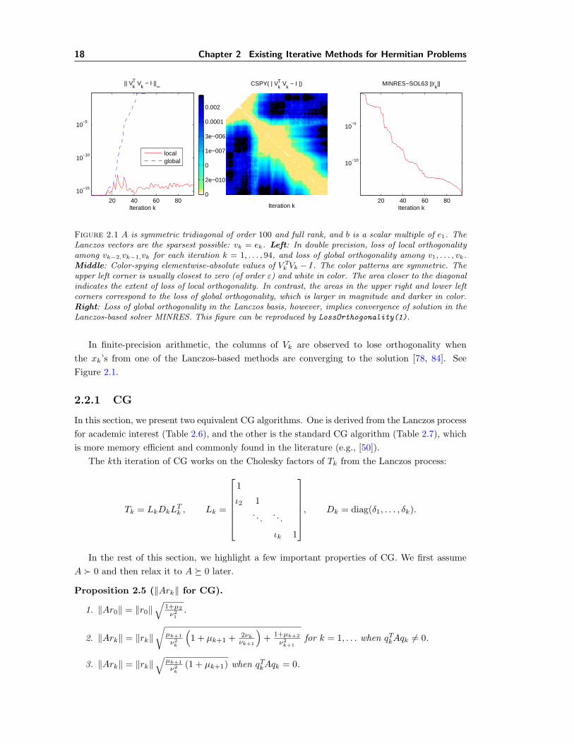
Figure 2.1 A is symmetric tridiagonal of order 100 and full rank, and b is a scalar multiple of e1. TheLanczos vectors are the sparsest possible: vk = ek. Left: In double precision, loss of local orthogonalityamong vk−2,vk−1,vk for each iteration k = 1, . . . , 94, and loss of global orthogonality among v1, . . . , vk.Middle: Color-spying elementwise-absolute values of V T
k Vk − I. The color patterns are symmetric. Theupper left corner is usually closest to zero (of order ε) and white in color. The area closer to the diagonalindicates the extent of loss of local orthogonality. In contrast, the areas in the upper right and lower leftcorners correspond to the loss of global orthogonality, which is larger in magnitude and darker in color.Right: Loss of global orthogonality in the Lanczos basis, however, implies convergence of solution in theLanczos-based solver MINRES. This figure can be reproduced by LossOrthogonality(1).
In finite-precision arithmetic, the columns of Vk are observed to lose orthogonality whenthe xk’s from one of the Lanczos-based methods are converging to the solution [78, 84]. SeeFigure 2.1.
2.2.1 CG
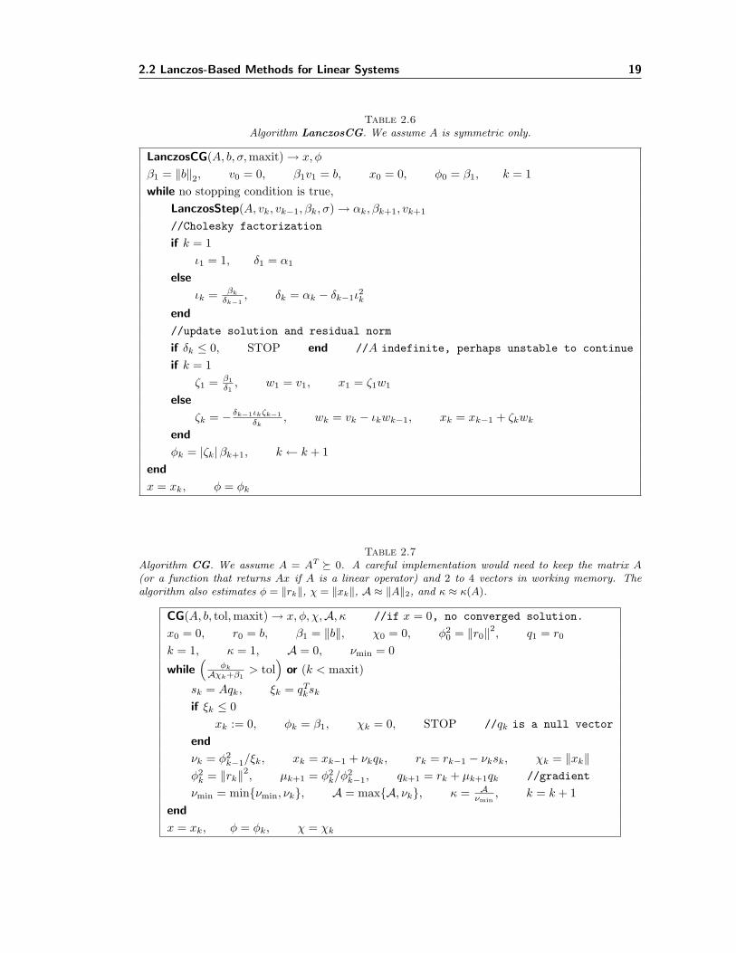
In this section, we present two equivalent CG algorithms. One is derived from the Lanczos processfor academic interest (Table 2.6), and the other is the standard CG algorithm (Table 2.7), whichis more memory efficient and commonly found in the literature (e.g., [50]).
The kth iteration of CG works on the Cholesky factors of Tk from the Lanczos process:
Tk = LkDkLTk , Lk =
1
ι2 1. . . . . .
ιk 1
, Dk = diag(δ1, . . . , δk).
In the rest of this section, we highlight a few important properties of CG. We first assumeA � 0 and then relax it to A � 0 later.
Proposition 2.5 (‖Ark‖ for CG).
1. ‖Ar0‖ = ‖r0‖√
1+µ2ν21
.
2. ‖Ark‖ = ‖rk‖√
µk+1
ν2k
(1 + µk+1 + 2νk
νk+1
)+ 1+µk+2
ν2k+1
for k = 1, . . . when qTkAqk 6= 0.
3. ‖Ark‖ = ‖rk‖√
µk+1
ν2k
(1 + µk+1) when qTkAqk = 0.
2.2 Lanczos-Based Methods for Linear Systems 19
Table 2.6Algorithm LanczosCG. We assume A is symmetric only.
LanczosCG(A, b, σ,maxit)→ x, φ
β1 = ‖b‖2, v0 = 0, β1v1 = b, x0 = 0, φ0 = β1, k = 1while no stopping condition is true,
LanczosStep(A, vk, vk−1, βk, σ)→ αk, βk+1, vk+1
//Cholesky factorization
if k = 1ι1 = 1, δ1 = α1
else
ιk = βk
δk−1, δk = αk − δk−1ι
2k
end
//update solution and residual norm
if δk ≤ 0, STOP end //A indefinite, perhaps unstable to continue
if k = 1ζ1 = β1
δ1, w1 = v1, x1 = ζ1w1
else
ζk = − δk−1ιkζk−1δk
, wk = vk − ιkwk−1, xk = xk−1 + ζkwk
end
φk = |ζk|βk+1, k ← k + 1end
x = xk, φ = φk
Table 2.7Algorithm CG. We assume A = AT � 0. A careful implementation would need to keep the matrix A(or a function that returns Ax if A is a linear operator) and 2 to 4 vectors in working memory. Thealgorithm also estimates φ = ‖rk‖, χ = ‖xk‖, A ≈ ‖A‖2, and κ ≈ κ(A).
CG(A, b, tol,maxit)→ x, φ, χ,A, κ //if x = 0, no converged solution.
20 Chapter 2 Existing Iterative Methods for Hermitian Problems
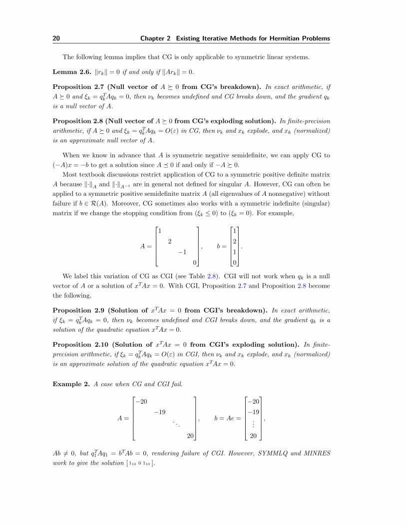
The following lemma implies that CG is only applicable to symmetric linear systems.
Lemma 2.6. ‖rk‖ = 0 if and only if ‖Ark‖ = 0.
Proposition 2.7 (Null vector of A � 0 from CG’s breakdown). In exact arithmetic, ifA � 0 and ξk = qTkAqk = 0, then νk becomes undefined and CG breaks down, and the gradient qkis a null vector of A.
Proposition 2.8 (Null vector of A � 0 from CG’s exploding solution). In finite-precisionarithmetic, if A � 0 and ξk = qTkAqk = O(ε) in CG, then νk and xk explode, and xk (normalized)is an approximate null vector of A.
When we know in advance that A is symmetric negative semidefinite, we can apply CG to(−A)x = −b to get a solution since A � 0 if and only if −A � 0.
Most textbook discussions restrict application of CG to a symmetric positive definite matrixA because ‖·‖A and ‖·‖A−1 are in general not defined for singular A. However, CG can often beapplied to a symmetric positive semidefinite matrix A (all eigenvalues of A nonnegative) withoutfailure if b ∈ R(A). Moreover, CG sometimes also works with a symmetric indefinite (singular)matrix if we change the stopping condition from (ξk ≤ 0) to (ξk = 0). For example,
A =
1
2
−1
0
, b =
1
2
1
0
.We label this variation of CG as CGI (see Table 2.8). CGI will not work when qk is a null
vector of A or a solution of xTAx = 0. With CGI, Proposition 2.7 and Proposition 2.8 becomethe following.
Proposition 2.9 (Solution of xTAx = 0 from CGI’s breakdown). In exact arithmetic,if ξk = qTkAqk = 0, then νk becomes undefined and CGI breaks down, and the gradient qk is asolution of the quadratic equation xTAx = 0.
Proposition 2.10 (Solution of xTAx = 0 from CGI’s exploding solution). In finite-precision arithmetic, if ξk = qTkAqk = O(ε) in CGI, then νk and xk explode, and xk (normalized)is an approximate solution of the quadratic equation xTAx = 0.
Example 2. A case when CG and CGI fail.
A =
−20
−19. . .
20
, b = Ae =
−20
−19...
20
,
Ab 6= 0, but qT1Aq1 = bTAb = 0, rendering failure of CGI. However, SYMMLQ and MINRESwork to give the solution [ 110 0 110 ].
2.2 Lanczos-Based Methods for Linear Systems 21
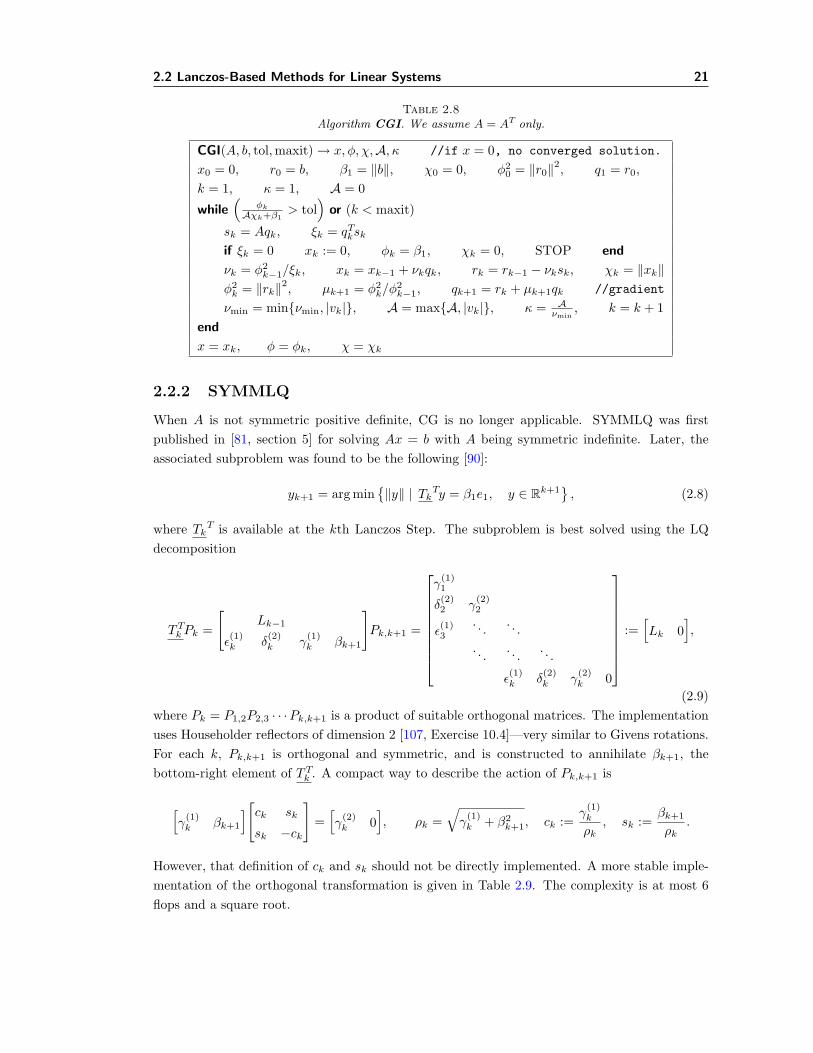
Table 2.8Algorithm CGI. We assume A = AT only.
CGI(A, b, tol,maxit)→ x, φ, χ,A, κ //if x = 0, no converged solution.
When A is not symmetric positive definite, CG is no longer applicable. SYMMLQ was firstpublished in [81, section 5] for solving Ax = b with A being symmetric indefinite. Later, theassociated subproblem was found to be the following [90]:
yk+1 = arg min{‖y‖ | TkTy = β1e1, y ∈ Rk+1
}, (2.8)
where TkT is available at the kth Lanczos Step. The subproblem is best solved using the LQdecomposition
TTkPk =
[Lk−1
ε(1)k δ
(2)k γ
(1)k βk+1
]Pk,k+1 =
γ(1)1
δ(2)2 γ
(2)2
ε(1)3
. . . . . .
. . . . . . . . .
ε(1)k δ
(2)k γ
(2)k 0
:=[Lk 0
],
(2.9)where Pk = P1,2P2,3 · · ·Pk,k+1 is a product of suitable orthogonal matrices. The implementationuses Householder reflectors of dimension 2 [107, Exercise 10.4]—very similar to Givens rotations.For each k, Pk,k+1 is orthogonal and symmetric, and is constructed to annihilate βk+1, thebottom-right element of TTk . A compact way to describe the action of Pk,k+1 is
[γ
(1)k βk+1
][ck sk
sk −ck
]=[γ
(2)k 0
], ρk =
√γ
(1)k + β2
k+1, ck :=γ
(1)k
ρk, sk :=
βk+1
ρk.
However, that definition of ck and sk should not be directly implemented. A more stable imple-mentation of the orthogonal transformation is given in Table 2.9. The complexity is at most 6flops and a square root.
22 Chapter 2 Existing Iterative Methods for Hermitian Problems
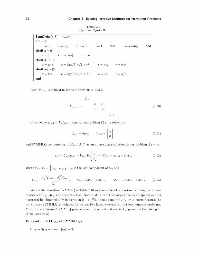
Table 2.9Algorithm SymOrtho.
SymOrtho(a, b)→ c, s, r
if b = 0s = 0, r = |a|, if a = 0, c = 1 else c = sign(a) end
elseif a = 0c = 0, s = sign(b), r = |b|
elseif |b| > |a|τ = a/b, s = sign(b)/
√1 + τ2, c = sτ , r = b/s
elseif |a| > |b|τ = b/a, c = sign(a)/
√1 + τ2, s = cτ , r = a/c
end
Each Pi,i+1 is defined in terms of previous ci and si:
Pi,i+1 :=
Ii−1
ci si
si −ciIk−i
. (2.10)
If we define yk+1 = Pkzk+1, then our subproblem (2.8) is solved by
Lkz = β1e1, zk+1 =
[zk
0
], (2.11)
and SYMMLQ computes xk in Kk+1(A, b) as an approximate solution to our problem Ax = b:
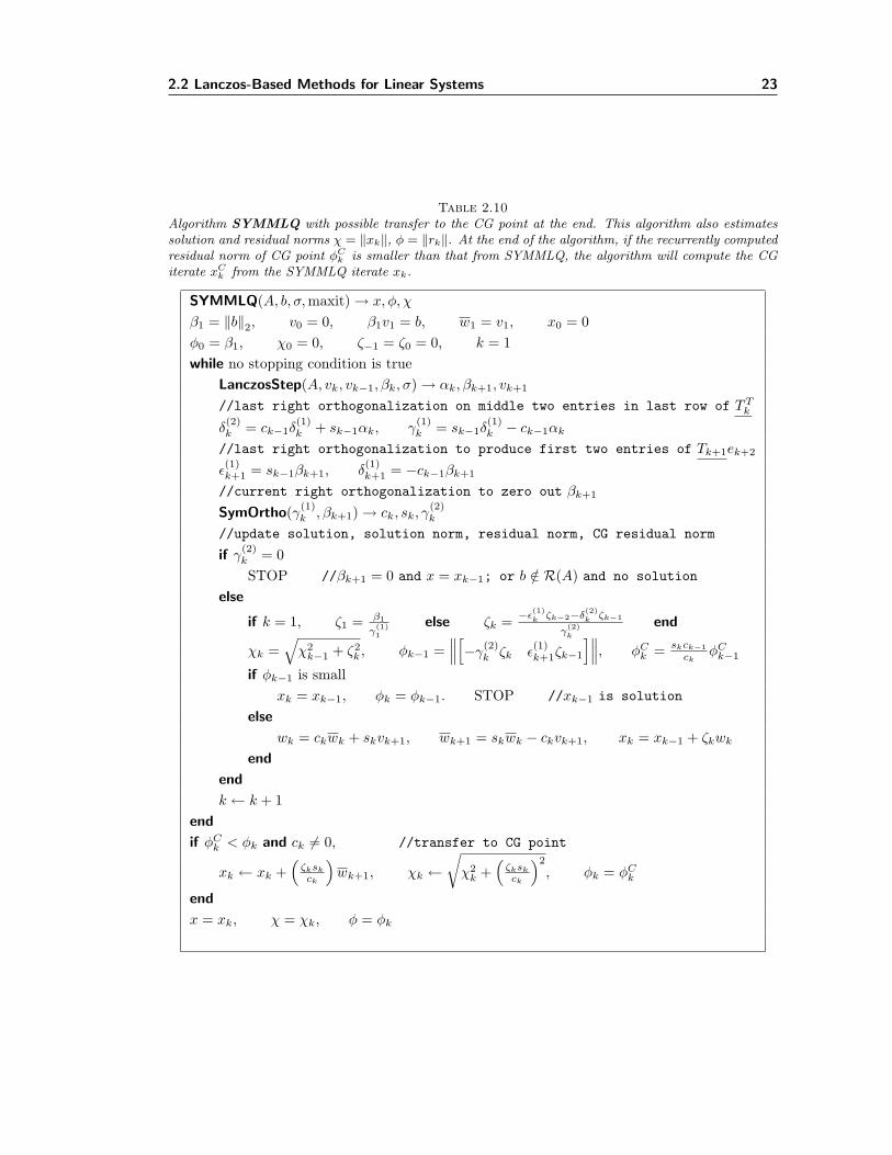
We list the algorithm SYMMLQ in Table 2.10 and give a list of properties including recurrencerelations for rk, Ark, and their 2-norms. Note that rk is not usually explicitly computed and itsnorm can be obtained only in iteration k + 1. We do not compute Ark or its norm because (aswe will see) SYMMLQ is designed for compatible linear systems but not least-squares problems.Most of the following SYMMLQ properties are presented and succinctly proved in the later partof [81, section 5].
Proposition 2.11 (rk of SYMMLQ).
1. r0 = β1v1 = b and ‖r0‖ = β1.
2.2 Lanczos-Based Methods for Linear Systems 23
Table 2.10Algorithm SYMMLQ with possible transfer to the CG point at the end. This algorithm also estimatessolution and residual norms χ = ‖xk‖, φ = ‖rk‖. At the end of the algorithm, if the recurrently computedresidual norm of CG point φC
k is smaller than that from SYMMLQ, the algorithm will compute the CGiterate xC
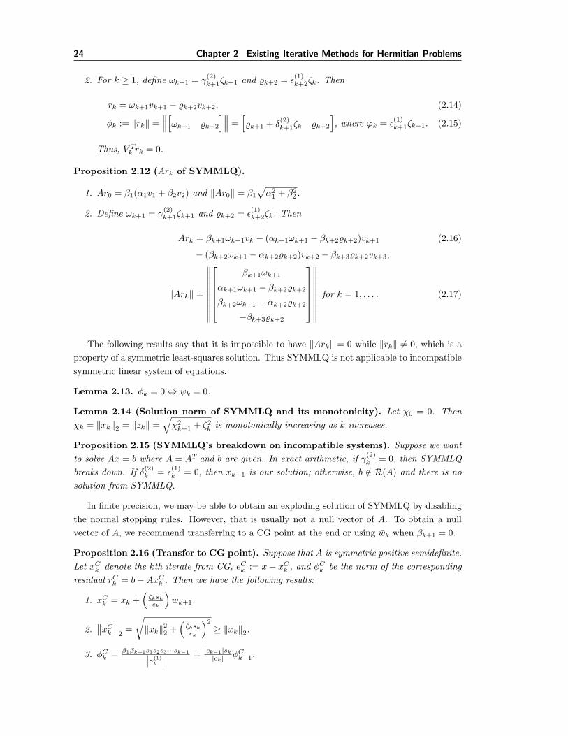
The following results say that it is impossible to have ‖Ark‖ = 0 while ‖rk‖ 6= 0, which is aproperty of a symmetric least-squares solution. Thus SYMMLQ is not applicable to incompatiblesymmetric linear system of equations.
Lemma 2.13. φk = 0⇔ ψk = 0.
Lemma 2.14 (Solution norm of SYMMLQ and its monotonicity). Let χ0 = 0. Thenχk = ‖xk‖2 = ‖zk‖ =
√χ2k−1 + ζ2
k is monotonically increasing as k increases.
Proposition 2.15 (SYMMLQ’s breakdown on incompatible systems). Suppose we wantto solve Ax = b where A = AT and b are given. In exact arithmetic, if γ(2)
k = 0, then SYMMLQbreaks down. If δ(2)k = ε
(1)k = 0, then xk−1 is our solution; otherwise, b /∈ R(A) and there is no
solution from SYMMLQ.
In finite precision, we may be able to obtain an exploding solution of SYMMLQ by disablingthe normal stopping rules. However, that is usually not a null vector of A. To obtain a nullvector of A, we recommend transferring to a CG point at the end or using wk when βk+1 = 0.
Proposition 2.16 (Transfer to CG point). Suppose that A is symmetric positive semidefinite.Let xCk denote the kth iterate from CG, eCk := x− xCk , and φCk be the norm of the correspondingresidual rCk = b−AxCk . Then we have the following results:
1. xCk = xk +(ζksk
ck
)wk+1.
2.∥∥xCk ∥∥2
=
√‖xk‖22 +
(ζksk
ck
)2
≥ ‖xk‖2.
3. φCk = β1βk+1s1s2s3···sk−1∣∣∣γ(1)k
∣∣∣ = |ck−1|sk
|ck| φCk−1.
2.2 Lanczos-Based Methods for Linear Systems 25
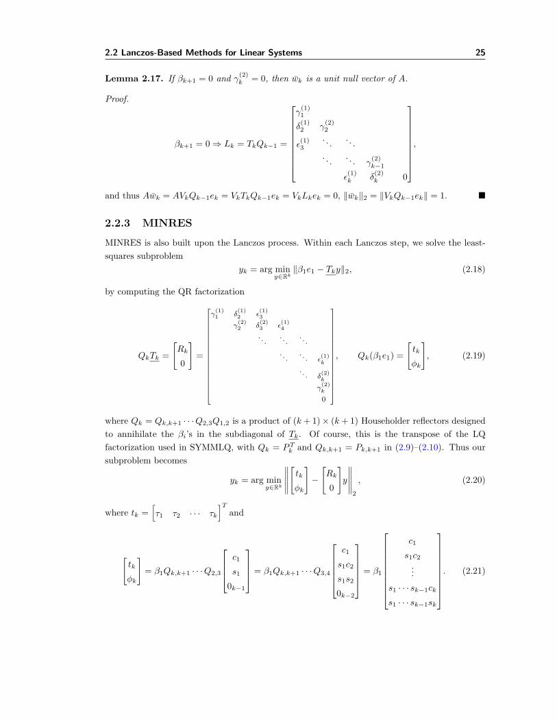
Lemma 2.17. If βk+1 = 0 and γ(2)k = 0, then wk is a unit null vector of A.
MINRES is also built upon the Lanczos process. Within each Lanczos step, we solve the least-squares subproblem
yk = arg miny∈Rk
‖β1e1 − Tky‖2, (2.18)
by computing the QR factorization
QkTk =
[Rk
0
]=
γ(1)1 δ
(1)2 ε
(1)3
γ(2)2 δ
(2)3 ε
(1)4
. . .. . .
. . .
. . .. . . ε
(1)k
. . . δ(2)k
γ(2)k
0
, Qk(β1e1) =
[tk
φk
], (2.19)
where Qk = Qk,k+1 · · ·Q2,3Q1,2 is a product of (k+ 1)× (k+ 1) Householder reflectors designedto annihilate the βi’s in the subdiagonal of Tk. Of course, this is the transpose of the LQfactorization used in SYMMLQ, with Qk = PTk and Qk,k+1 = Pk,k+1 in (2.9)–(2.10). Thus oursubproblem becomes
yk = arg miny∈Rk
∥∥∥∥∥[tk
φk
]−
[Rk
0
]y
∥∥∥∥∥2
, (2.20)
where tk =[τ1 τ2 · · · τk
]Tand
[tk
φk
]= β1Qk,k+1 · · ·Q2,3
c1
s1
0k−1
= β1Qk,k+1 · · ·Q3,4
c1
s1c2
s1s2
0k−2
= β1
c1
s1c2...
s1 · · · sk−1ck
s1 · · · sk−1sk
. (2.21)
26 Chapter 2 Existing Iterative Methods for Hermitian Problems
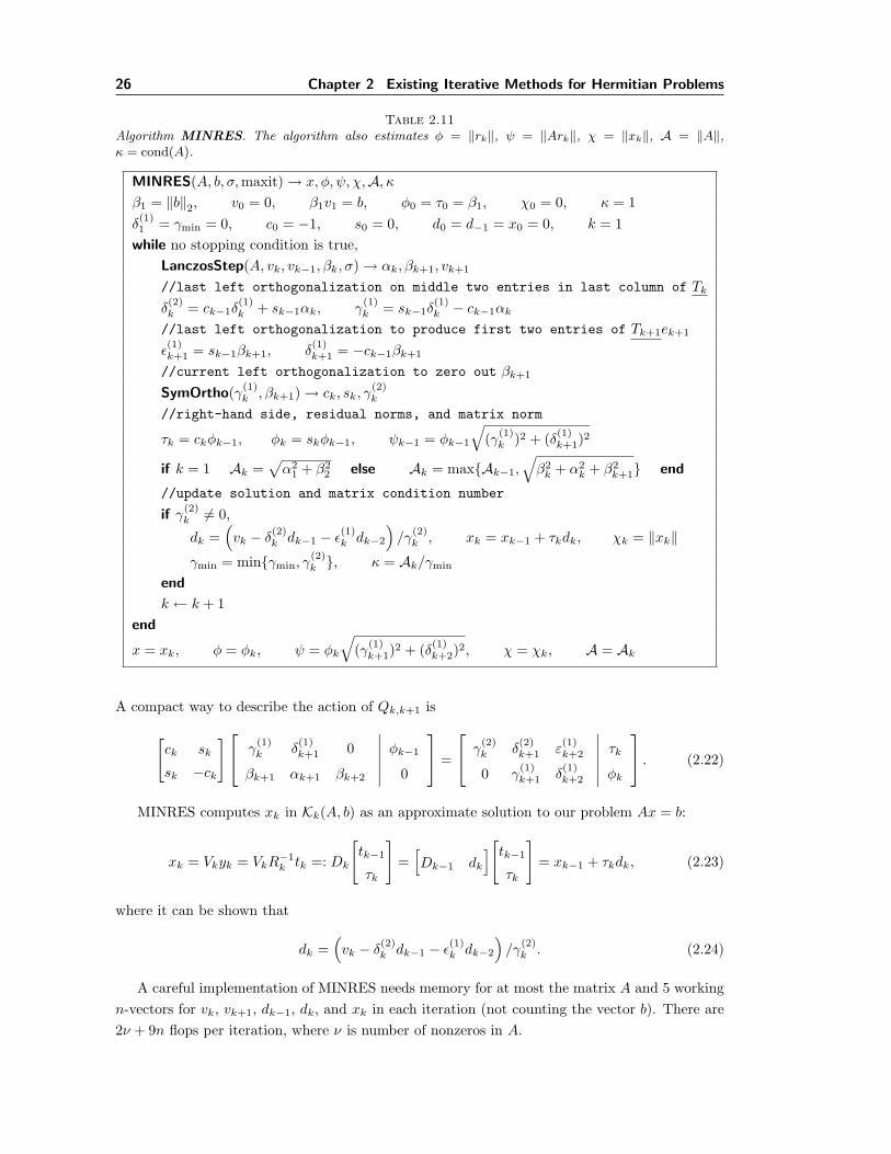
Table 2.11Algorithm MINRES. The algorithm also estimates φ = ‖rk‖, ψ = ‖Ark‖, χ = ‖xk‖, A = ‖A‖,κ = cond(A).
while no stopping condition is true,LanczosStep(A, vk, vk−1, βk, σ)→ αk, βk+1, vk+1
//last left orthogonalization on middle two entries in last column of Tk
δ(2)k = ck−1δ
(1)k + sk−1αk, γ
(1)k = sk−1δ
(1)k − ck−1αk
//last left orthogonalization to produce first two entries of Tk+1ek+1
ε(1)k+1 = sk−1βk+1, δ
(1)k+1 = −ck−1βk+1
//current left orthogonalization to zero out βk+1
SymOrtho(γ(1)k , βk+1)→ ck, sk, γ
(2)k
//right-hand side, residual norms, and matrix norm
τk = ckφk−1, φk = skφk−1, ψk−1 = φk−1
√(γ(1)k )2 + (δ(1)k+1)2
if k = 1 Ak =√α2
1 + β22 else Ak = max{Ak−1,
√β2k + α2
k + β2k+1} end
//update solution and matrix condition number
if γ(2)k 6= 0,
dk =(vk − δ(2)k dk−1 − ε(1)k dk−2
)/γ
(2)k , xk = xk−1 + τkdk, χk = ‖xk‖
γmin = min{γmin, γ(2)k }, κ = Ak/γmin
end
k ← k + 1end
x = xk, φ = φk, ψ = φk
√(γ(1)k+1)2 + (δ(1)k+2)2, χ = χk, A = Ak
A compact way to describe the action of Qk,k+1 is
[ck sk
sk −ck
] γ(1)k δ
(1)k+1 0
βk+1 αk+1 βk+2
∣∣∣∣∣∣ φk−1
0
=
γ(2)k δ
(2)k+1 ε
(1)k+2
0 γ(1)k+1 δ
(1)k+2
∣∣∣∣∣∣ τkφk . (2.22)
MINRES computes xk in Kk(A, b) as an approximate solution to our problem Ax = b:
xk = Vkyk = VkR−1k tk =: Dk
[tk−1
τk
]=[Dk−1 dk
][tk−1
τk
]= xk−1 + τkdk, (2.23)
where it can be shown that
dk =(vk − δ(2)k dk−1 − ε(1)k dk−2
)/γ
(2)k . (2.24)
A careful implementation of MINRES needs memory for at most the matrix A and 5 workingn-vectors for vk, vk+1, dk−1, dk, and xk in each iteration (not counting the vector b). There are2ν + 9n flops per iteration, where ν is number of nonzeros in A.
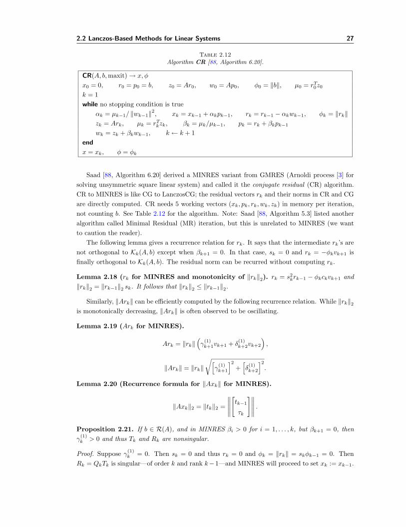
Saad [88, Algorithm 6.20] derived a MINRES variant from GMRES (Arnoldi process [3] forsolving unsymmetric square linear system) and called it the conjugate residual (CR) algorithm.CR to MINRES is like CG to LanczosCG; the residual vectors rk and their norms in CR and CGare directly computed. CR needs 5 working vectors (xk, pk, rk, wk, zk) in memory per iteration,not counting b. See Table 2.12 for the algorithm. Note: Saad [88, Algorithm 5.3] listed anotheralgorithm called Minimal Residual (MR) iteration, but this is unrelated to MINRES (we wantto caution the reader).
The following lemma gives a recurrence relation for rk. It says that the intermediate rk’s arenot orthogonal to Kk(A, b) except when βk+1 = 0. In that case, sk = 0 and rk = −φkvk+1 isfinally orthogonal to Kk(A, b). The residual norm can be recurred without computing rk.
Lemma 2.18 (rk for MINRES and monotonicity of ‖rk‖2). rk = s2krk−1 − φkckvk+1 and‖rk‖2 = ‖rk−1‖2 sk. It follows that ‖rk‖2 ≤ ‖rk−1‖2.
Similarly, ‖Ark‖ can be efficiently computed by the following recurrence relation. While ‖rk‖2is monotonically decreasing, ‖Ark‖ is often observed to be oscillating.
Lemma 2.19 (Ark for MINRES).
Ark = ‖rk‖(γ
(1)k+1vk+1 + δ
(1)k+2vk+2
),
‖Ark‖ = ‖rk‖√[
γ(1)k+1
]2+[δ(1)k+2
]2.
Lemma 2.20 (Recurrence formula for ‖Axk‖ for MINRES).
‖Axk‖2 = ‖tk‖2 =
∥∥∥∥∥[tk−1
τk
]∥∥∥∥∥ .Proposition 2.21. If b ∈ R(A), and in MINRES βi > 0 for i = 1, . . . , k, but βk+1 = 0, thenγ
(1)k > 0 and thus Tk and Rk are nonsingular.
Proof. Suppose γ(1)k = 0. Then sk = 0 and thus rk = 0 and φk = ‖rk‖ = skφk−1 = 0. Then
Rk = QkTk is singular—of order k and rank k−1—and MINRES will proceed to set xk := xk−1.
28 Chapter 2 Existing Iterative Methods for Hermitian Problems
It follows that rk := rk−1 and φk = φk−1 = 0. However, this contradicts the fact that MINREShad not stopped at the (k − 1)th iteration. �
Corollary 2.22. If in MINRES βi > 0 for i = 1, . . . , k, and βk+1 = 0, and γ(1)k = 0, then Tk
and Rk are singular (both of order k and rank k − 1) and b /∈ R(A).
In the following, we review the definition of minimum-length solution or pseudoinverse solutionfor a linear system. Then we prove that MINRES returns the unique minimum-length solutionfor any symmetric compatible (possibly singular) system.
Definition 2.23 (Moore-Penrose conditions and pseudoinverse [50]). Given any m× nmatrix A, X is the pseudoinverse of A if it satisfies the four Moore-Penrose conditions:
1. AXA = A.
2. XAX = X.
3. (AX)H = AX.
4. (XA)H = XA.
Theorem 2.24 (Existence and uniqueness of the pseudoinverse). The pseudoinverse ofa matrix always exists and is unique.
If A is square and nonsingular, then A†, the pseudoinverse of A, is the matrix inverse A−1.Even if A is square and nonsingular, we rarely compute A−1. Instead, we would compute
say the LU decomposition PA = LU or QR decomposition A = QR. If we want the solutionof Ax = b, we do not compute x = A−1b but instead, solve the triangular systems Ly = Pb
and Ux = y if we have computed LU decomposition of A, or Rx = QTb in the case of QRdecomposition. Likewise, we rarely compute the pseudoinverse of A. It is mainly an analyticaltool. If A is singular, A−1 does not exist, but Ax = b may have a solution. In that case, there areinfinitely many solutions. In some applications we want the unique minimum-length solution,which could be written in terms of the pseudoinverse of A: x† = A†b. However, to compute x†, wewould not compute A†. Instead we could compute some rank-revealing factorization of A such asthe reduced singular value decomposition A = UΣV T, where U and V have orthogonal columnsand Σ is diagonal with positive entries. Then the minimum-length solution is x† = V Σ−1UTb.
Theorem 2.25. If b ∈ R(A), and in MINRES βi > 0 for i = 1, . . . , k, but βk+1 = 0, then xk isthe pseudoinverse solution of Ax = b.
Proof. We know that span(v1, . . . , vk) ⊆ R(A). However, we assume span(v1, . . . , vk) = R(A).Without this assumption, the result is still true but the proof will be more complicated.
By Proposition 2.21, when βk+1 = 0, R−1k exists. Moreover,
xk = Vkyk = VkR−1k tk = VkR
−1k β1Qk−1e1 = VkR
−1k Qk−1V
Tk b. (2.25)
Thus, we define
A\ := VkR−1k Qk−1V
Tk = VkT
−1k V Tk since Qk−1Tk = Rk.
2.3 Existing Iterative Methods for Hermitian Least-Squares 29
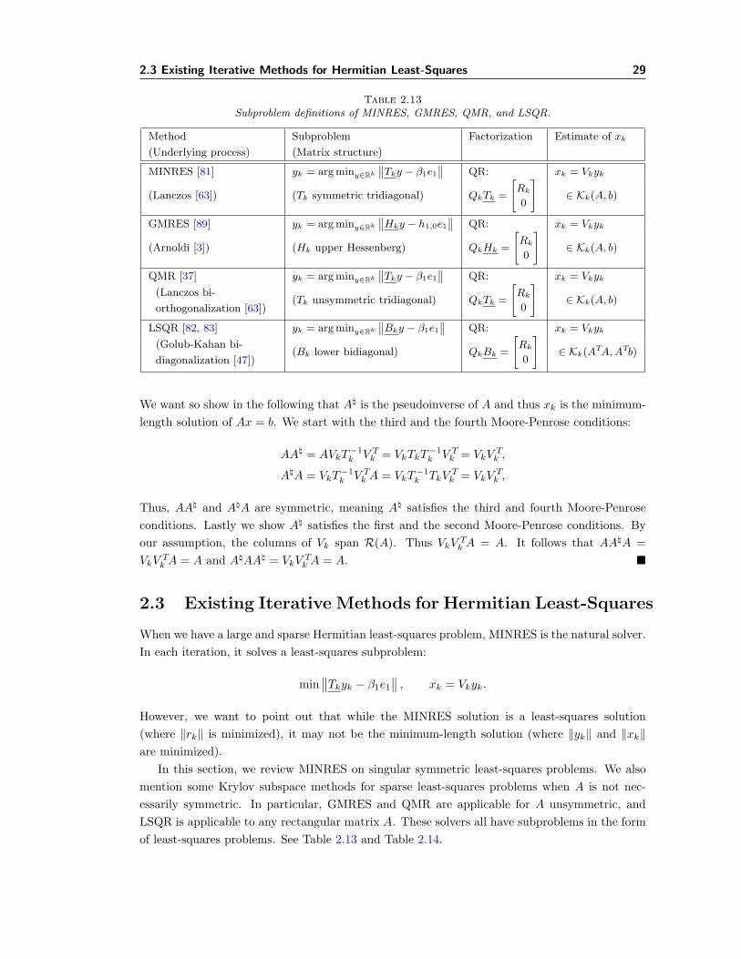
Table 2.13Subproblem definitions of MINRES, GMRES, QMR, and LSQR.
We want so show in the following that A\ is the pseudoinverse of A and thus xk is the minimum-length solution of Ax = b. We start with the third and the fourth Moore-Penrose conditions:
AA\ = AVkT−1k V Tk = VkTkT
−1k V Tk = VkV
Tk ,
A\A = VkT−1k V Tk A = VkT
−1k TkV
Tk = VkV
Tk ,
Thus, AA\ and A\A are symmetric, meaning A\ satisfies the third and fourth Moore-Penroseconditions. Lastly we show A\ satisfies the first and the second Moore-Penrose conditions. Byour assumption, the columns of Vk span R(A). Thus VkV Tk A = A. It follows that AA\A =VkV
Tk A = A and A\AA\ = VkV
Tk A = A. �
2.3 Existing Iterative Methods for Hermitian Least-Squares
When we have a large and sparse Hermitian least-squares problem, MINRES is the natural solver.In each iteration, it solves a least-squares subproblem:
min∥∥Tkyk − β1e1
∥∥ , xk = Vkyk.
However, we want to point out that while the MINRES solution is a least-squares solution(where ‖rk‖ is minimized), it may not be the minimum-length solution (where ‖yk‖ and ‖xk‖are minimized).
In this section, we review MINRES on singular symmetric least-squares problems. We alsomention some Krylov subspace methods for sparse least-squares problems when A is not nec-essarily symmetric. In particular, GMRES and QMR are applicable for A unsymmetric, andLSQR is applicable to any rectangular matrix A. These solvers all have subproblems in the formof least-squares problems. See Table 2.13 and Table 2.14.
30 Chapter 2 Existing Iterative Methods for Hermitian Problems
Table 2.14Bases and subproblem solutions in MINRES, GMRES, QMR, and LSQR.
Method New basis zk Estimate of xk
MINRES Dk := VkR−1k Rkzk = β1
[Ik 0
]Qke1 xk = Dkzk
GMRES – – xk = Vkyk
QMR Wk := VkR−1k Rkzk = β1
[Ik 0
]Qke1 xk = Wkzk
LSQR Wk := VkR−1k Rkzk = β1
[Ik 0
]Qke1 xk = Wkzk
2.3.1 MINRES
In this section, we want to show that MINRES produces a generalized-inverse solution when wehave a least-squares problem min ‖Ax− b‖, where A is singular and b /∈ R(A).
The pseudoinverse is a kind of generalized inverse and there are other kinds (see [7]). Gener-alized inverses of a rank-deficient matrix may not be unique.
Definition 2.26 (Generalized inverses). For i = 1, 2, 3, 4, X is the {i}-inverse of an m× nmatrix A if it satisfies the ith Moore-Penrose condition. Likewise, X is the {i, j}-inverse of A ifit satisfies both the ith and jth Moore-Penrose conditions. Lastly, X is the {i, j, k}-inverse of Aif it satisfies the ith, jth, and kth Moore-Penrose conditions.
Theorem 2.27. Consider a symmetric linear least-squares problem min ‖Ax− b‖, with A = AT
singular and b /∈ R(A). If βi 6= 0 for i = 1, . . . , k, βk+1 = γ(1)k = 0 and ‖Ark‖ = 0, then
xk := xk−1 is a {2, 3}-inverse solution, meaning xk = Xb for some X being a {2, 3}-inverseof A. Moreover, xk is a {1, 2, 3}-inverse solution if the columns of Vk span R(A).
Proof. If βk+1 = 0 and also γ(1)k = 0 in (2.20), then iteration k is going to be our last iteration in
the Lanczos process, and (2.20) becomes the following underdetermined least-squares problem:
min
∥∥∥∥∥∥∥∥Rk−1 s
0 0
0
[yk−1
ηk
]−
tk−1
φk−1
0
∥∥∥∥∥∥∥∥ = min
∥∥∥∥∥[Rk−1 s][yk−1
ηk
]−
[tk−1
φk−1
]∥∥∥∥∥ ,
wheres :=
[ε(1)k ek−2
δ(2)k
]6= 0 since ε
(1)k = sk−2βk.
We choose to set ηk = 0, thus simplifying the subproblem to Rk−1yk−1 = tk−1, which is actuallyour previous subproblem in the (k − 1)th iteration. Therefore
xk := xk−1 = Vk−1yk−1 = Vkyk, where yk :=
[yk−1
0
], (2.26)
‖rk‖ = ‖rk−1‖ = φk−1 > 0 (or we would have stopped in the (k − 1)th iteration), (2.27)
‖Ark‖ = ‖Ark−1‖ = ‖rk−1‖√[
γ(2)k
]2+[δ(2)k+1
]2= 0, (2.28)
since βk+1 = γ(1)k = 0 =⇒ γ
(2)k = δ
(2)k+1 = 0 by (2.22), confirming that xk−1 is our least-squares
2.3 Existing Iterative Methods for Hermitian Least-Squares 31
solution. Moreover, by (2.26)
xk = Vkyk = Vk
[yk−1
0
]= Vk
[R−1k−1 0
0 0
][tk−1
φk−1
]= Vk
[R−1k−1 0
0 0
](β1Qk−1e1) (2.29)
= VkR]kQk−1V
Tk b, where R]k :=
[R−1k−1 0
0 0
](2.30)
= A]b, where A] := VkR]kQk−1V
Tk . (2.31)
We will check if A] satisfies any of the Moore-Penrose conditions in the following. Recall thatwhen βk+1 = γ
(1)k = 0, then
AVk = Vk+1Tk = VkTk = VkQTk−1Rk, Rk =
[Rk−1 s
0 0
], V Tk AVk = Tk. (2.32)
First, we show that A] satisfies the third but not the fourth Moore-Penrose conditions:
AA] = AVkR]kQk−1V
Tk = VkQ
Tk−1RkR
]kQk−1V
Tk = VkQ
Tk−1
[Ik−1
0
]Qk−1V
Tk , (2.33)
A]A = VkR]kQk−1V
Tk A = VkR
]
kQk−1TkVTk = VkR
]kRkV
Tk , (2.34)
so that AA] is symmetric, but(R]kRk
)T=[Ik−1 R
−1k−1s
0 0
]T6= R]kRk, since s 6= 0 by (2.27). Thus
A]A is not symmetric.Next, we check the first Moore-Penrose condition:
AA]A = (AVk)R]kQk−1
(V Tk A
)=(VkQ
Tk−1Rk
)R]kQk−1
(TkV
Tk
)by (2.31) – (2.32) (2.35)
= VkQTk−1RkR
]kRkV
Tk = VkQ
Tk−1RkV
Tk since it is easy to verify RkR
]kRk = Rk (2.36)
= AVkVTk by (2.32) (2.37)
= A(Vk,R + v1,N cT )(Vk,R + v1,N c
T )T, where Vk,R =[v1,R · · · vk,R
]by (2.2) (2.38)
= AVk,RVTk,R= A if the columns of Vk,R span R(A). (2.39)
Lastly, A] satisfies the second Moore-Penrose condition:
A]AA] = VkR]kRkV
Tk VkR
]kQk−1V
Tk by (2.34) (2.40)
= VkR]kRkR
]kQk−1V
Tk = VkR
]kQk−1V
Tk = A] since R]kRkR
]k = R]k. (2.41)
�
Example 3. MINRES on min ‖Ax − b‖ with A =[
1 0 00 1 00 0 0
], b =
[111
]. The minimum-length
solution is x† =[
110
]and the residuals are r† = b−Ax† =
[001
]and Ar† = 0. However, MINRES
returns a least-squares solution x] =[
111
]with residuals r] = b− Ax] =
[001
]and Ar] = 0. Thus
we need a new stopping condition ‖Ark‖ ≤ tol and a modified MINRES algorithm to get theminimum-length solution.
32 Chapter 2 Existing Iterative Methods for Hermitian Problems
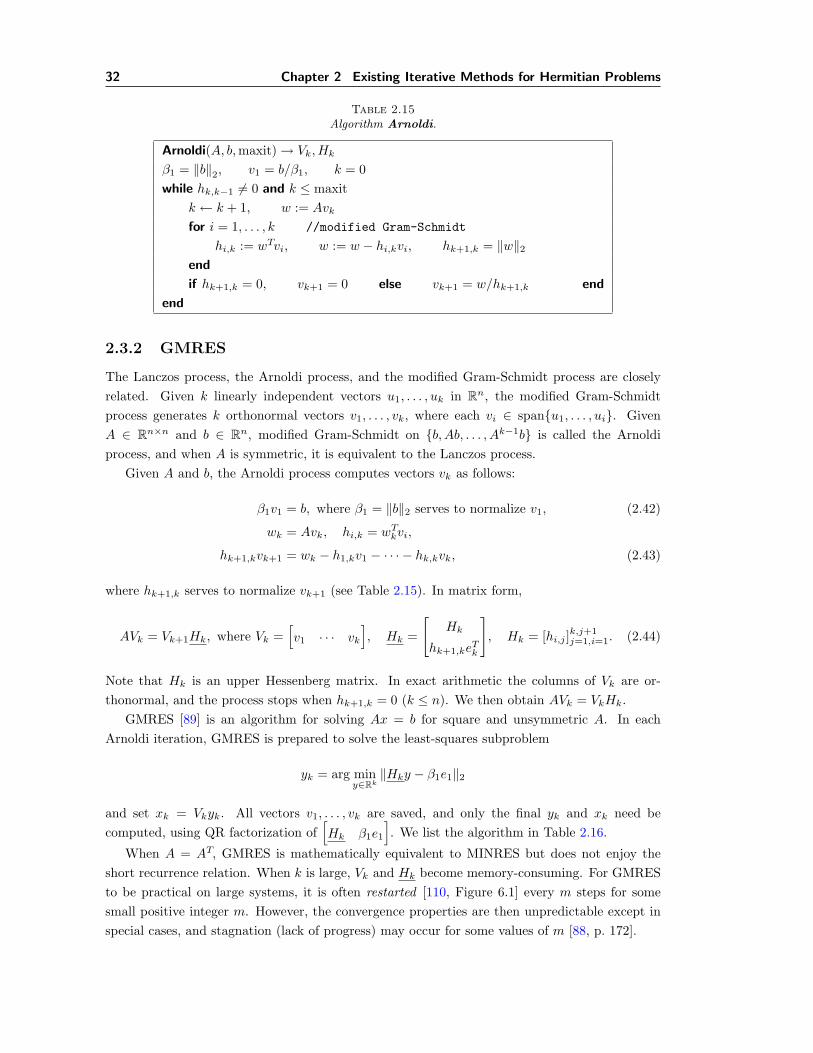
Table 2.15Algorithm Arnoldi.
Arnoldi(A, b,maxit)→ Vk,Hk
β1 = ‖b‖2, v1 = b/β1, k = 0while hk,k−1 6= 0 and k ≤ maxit
k ← k + 1, w := Avk
for i = 1, . . . , k //modified Gram-Schmidt
hi,k := wTvi, w := w − hi,kvi, hk+1,k = ‖w‖2end
if hk+1,k = 0, vk+1 = 0 else vk+1 = w/hk+1,k end
end
2.3.2 GMRES
The Lanczos process, the Arnoldi process, and the modified Gram-Schmidt process are closelyrelated. Given k linearly independent vectors u1, . . . , uk in Rn, the modified Gram-Schmidtprocess generates k orthonormal vectors v1, . . . , vk, where each vi ∈ span{u1, . . . , ui}. GivenA ∈ Rn×n and b ∈ Rn, modified Gram-Schmidt on {b, Ab, . . . , Ak−1b} is called the Arnoldiprocess, and when A is symmetric, it is equivalent to the Lanczos process.
Given A and b, the Arnoldi process computes vectors vk as follows:
β1v1 = b, where β1 = ‖b‖2 serves to normalize v1, (2.42)
wk = Avk, hi,k = wTkvi,
hk+1,kvk+1 = wk − h1,kv1 − · · · − hk,kvk, (2.43)
where hk+1,k serves to normalize vk+1 (see Table 2.15). In matrix form,
AVk = Vk+1Hk, where Vk =[v1 · · · vk
], Hk =
[Hk
hk+1,keTk
], Hk = [hi,j ]
k,j+1j=1,i=1. (2.44)
Note that Hk is an upper Hessenberg matrix. In exact arithmetic the columns of Vk are or-thonormal, and the process stops when hk+1,k = 0 (k ≤ n). We then obtain AVk = VkHk.
GMRES [89] is an algorithm for solving Ax = b for square and unsymmetric A. In eachArnoldi iteration, GMRES is prepared to solve the least-squares subproblem
yk = arg miny∈Rk
‖Hky − β1e1‖2
and set xk = Vkyk. All vectors v1, . . . , vk are saved, and only the final yk and xk need becomputed, using QR factorization of
[Hk β1e1
]. We list the algorithm in Table 2.16.
When A = AT, GMRES is mathematically equivalent to MINRES but does not enjoy theshort recurrence relation. When k is large, Vk and Hk become memory-consuming. For GMRESto be practical on large systems, it is often restarted [110, Figure 6.1] every m steps for somesmall positive integer m. However, the convergence properties are then unpredictable except inspecial cases, and stagnation (lack of progress) may occur for some values of m [88, p. 172].
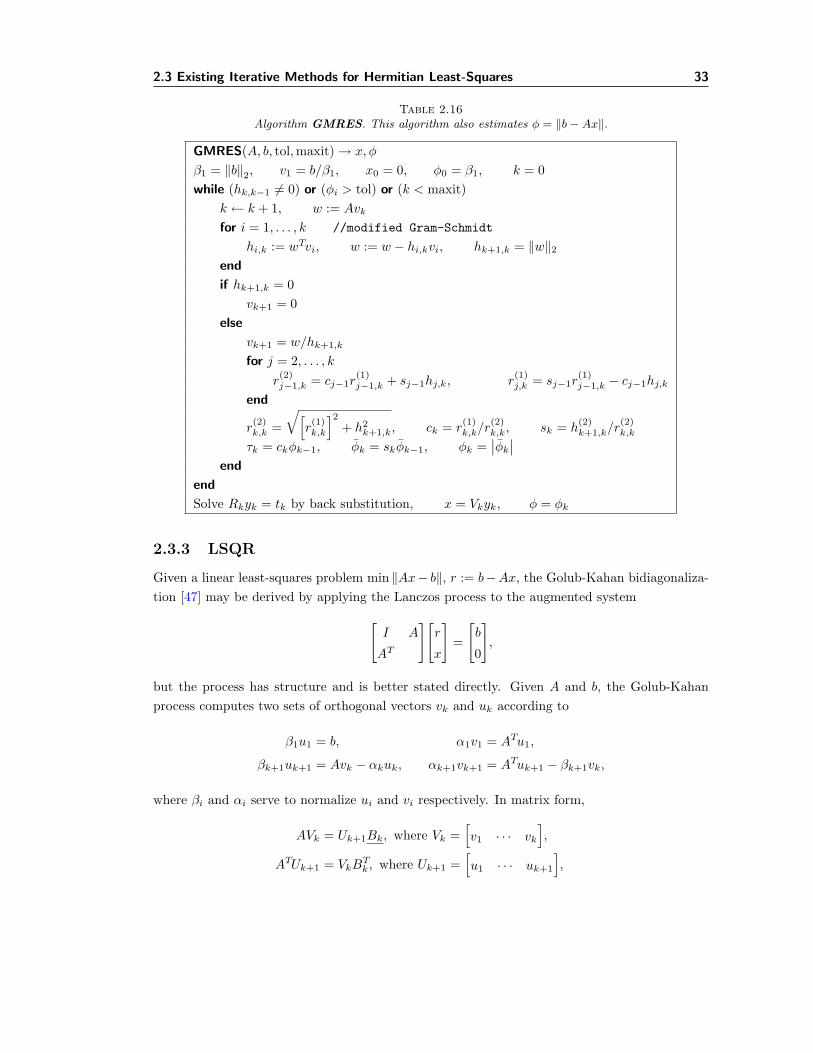
2.3 Existing Iterative Methods for Hermitian Least-Squares 33
Table 2.16Algorithm GMRES. This algorithm also estimates φ = ‖b−Ax‖.
GMRES(A, b, tol,maxit)→ x, φ
β1 = ‖b‖2, v1 = b/β1, x0 = 0, φ0 = β1, k = 0while (hk,k−1 6= 0) or (φi > tol) or (k < maxit)
k ← k + 1, w := Avk
for i = 1, . . . , k //modified Gram-Schmidt
hi,k := wTvi, w := w − hi,kvi, hk+1,k = ‖w‖2end
if hk+1,k = 0vk+1 = 0
else
vk+1 = w/hk+1,k
for j = 2, . . . , kr(2)j−1,k = cj−1r
(1)j−1,k + sj−1hj,k, r
(1)j,k = sj−1r
(1)j−1,k − cj−1hj,k
end
r(2)k,k =
√[r(1)k,k
]2+ h2
k+1,k, ck = r(1)k,k/r
(2)k,k, sk = h
(2)k+1,k/r
(2)k,k
τk = ckφk−1, φk = skφk−1, φk =∣∣φk∣∣
end
end
Solve Rkyk = tk by back substitution, x = Vkyk, φ = φk
2.3.3 LSQR
Given a linear least-squares problem min ‖Ax− b‖, r := b−Ax, the Golub-Kahan bidiagonaliza-tion [47] may be derived by applying the Lanczos process to the augmented system[
I A
AT
][r
x
]=
[b
0
],
but the process has structure and is better stated directly. Given A and b, the Golub-Kahanprocess computes two sets of orthogonal vectors vk and uk according to
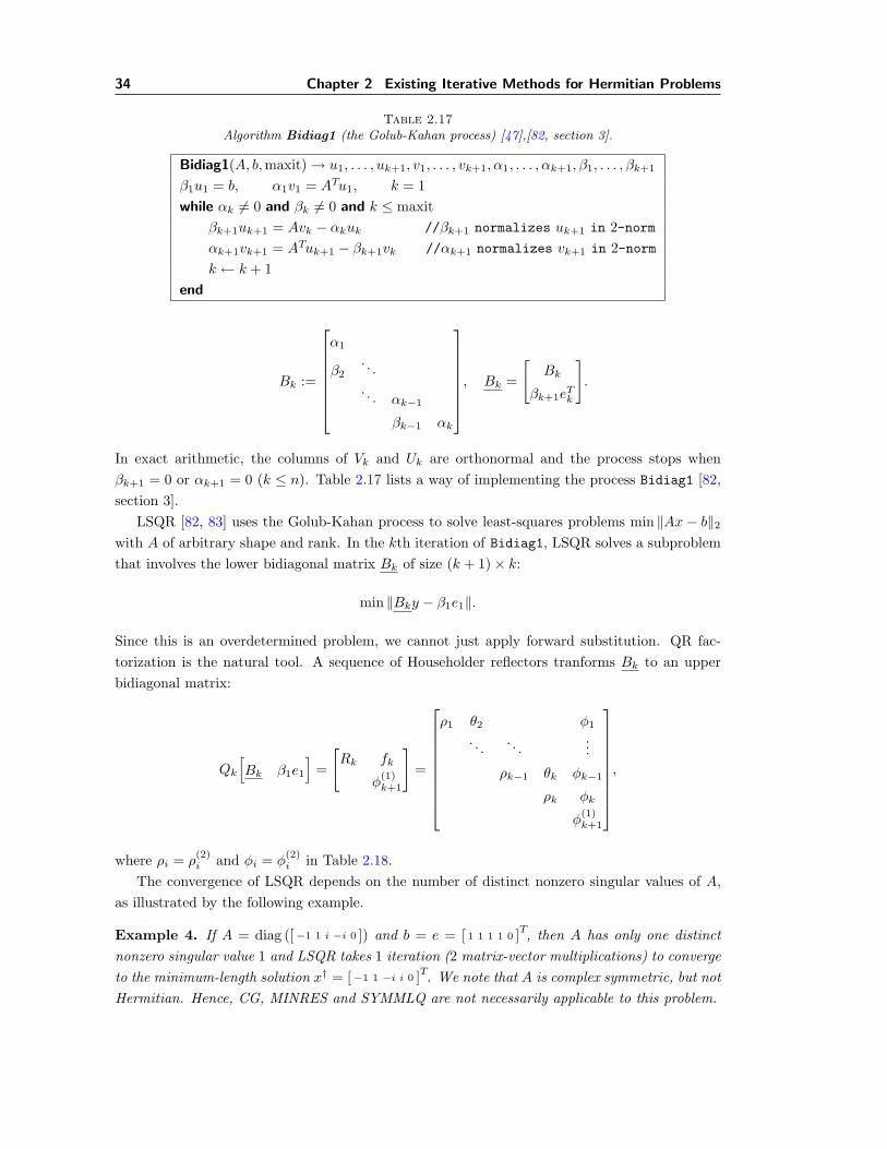
β1u1 = b, α1v1 = ATu1, k = 1while αk 6= 0 and βk 6= 0 and k ≤ maxit
βk+1uk+1 = Avk − αkuk //βk+1 normalizes uk+1 in 2-normαk+1vk+1 = ATuk+1 − βk+1vk //αk+1 normalizes vk+1 in 2-normk ← k + 1
end
Bk :=
α1
β2. . .. . . αk−1
βk−1 αk
, Bk =
[Bk
βk+1eTk
].
In exact arithmetic, the columns of Vk and Uk are orthonormal and the process stops whenβk+1 = 0 or αk+1 = 0 (k ≤ n). Table 2.17 lists a way of implementing the process Bidiag1 [82,section 3].
LSQR [82, 83] uses the Golub-Kahan process to solve least-squares problems min ‖Ax − b‖2with A of arbitrary shape and rank. In the kth iteration of Bidiag1, LSQR solves a subproblemthat involves the lower bidiagonal matrix Bk of size (k + 1)× k:
min ‖Bky − β1e1‖.
Since this is an overdetermined problem, we cannot just apply forward substitution. QR fac-torization is the natural tool. A sequence of Householder reflectors tranforms Bk to an upperbidiagonal matrix:
Qk
[Bk β1e1
]=
[Rk fk
φ(1)k+1
]=
ρ1 θ2 φ1
. . . . . ....
ρk−1 θk φk−1
ρk φk
φ(1)k+1
,
where ρi = ρ(2)i and φi = φ
(2)i in Table 2.18.
The convergence of LSQR depends on the number of distinct nonzero singular values of A,as illustrated by the following example.
Example 4. If A = diag ([−1 1 i −i 0 ]) and b = e = [ 1 1 1 1 0 ]T, then A has only one distinctnonzero singular value 1 and LSQR takes 1 iteration (2 matrix-vector multiplications) to convergeto the minimum-length solution x† = [−1 1 −i i 0 ]T. We note that A is complex symmetric, but notHermitian. Hence, CG, MINRES and SYMMLQ are not necessarily applicable to this problem.
2.4 Stopping Conditions and Norm Estimates 35
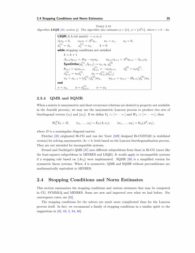
Table 2.18Algorithm LSQR [82, section 4]. This algorithm also estimates φ = ‖r‖, ψ = ‖ATr‖, where r = b−Ax.
LSQR(A, b, tol,maxit)→ x, φ, ψ
β1u1 = b, α1v1 = ATu1, w1 = v1, x0 = 0,φ
(1)1 = β1, ρ
(1)1 = α1, k = 0
while stopping conditions not satisfiedk = k + 1βk+1uk+1 = Avk − αkuk, αk+1vk+1 = ATuk+1 − βk+1vk
SymOrtho(ρ(1)k , βk+1)→ ck, sk, ρ
(2)k
θk+1 = skαk+1, ρ(1)k+1 = −ckαk+1, φ
(2)k = ckφ
(1)k ,
φ(1)k+1 = skφ
(1)k , ψk = φ
(1)k+1|ρ
(1)k+1|
xk = xk−1 + (φ(2)k /ρ
(2)k )wk, wk+1 = vk+1 − (θk+1/ρ
(2)k )wk
end
x = xk, φ = φ(1)k+1, ψ = ψk
2.3.4 QMR and SQMR
When a matrix is unsymmetric and short recurrence relations are desired (a property not availablein the Arnoldi process), we may use the unsymmetric Lanczos process to produce two sets ofbiorthogonal vectors {vi} and {wi}. If we define Vk := [ v1 ... vk ] and Wk := [w1 ... wk ], then
where D is a nonsingular diagonal matrix.Fletcher [35] originated Bi-CG and van der Vorst [109] designed Bi-CGSTAB (a stabilized
version) for solving unsymmetric Ax = b, both based on the Lanczos biorthogonalization process.They are not intended for incompatible systems.
Freund and Nachtigal’s QMR [37] uses different subproblems from those in Bi-CG (more likethe least-squares subproblems in MINRES and LSQR). It would apply to incompatible systemsif a stopping rule based on ‖Ark‖ were implemented. SQMR [38] is a simplified version forsymmetric linear systems. When A is symmetric, QMR and SQMR without preconditioner aremathematically equivalent to MINRES.
2.4 Stopping Conditions and Norm Estimates
This section summarizes the stopping conditions and various estimates that may be computedin CG, SYMMLQ and MINRES. Some are new and improved over what we had before. Forconvergence rates, see [62].
The stopping conditions for the solvers are much more complicated than for the Lanczosprocess itself. In fact, we recommend a family of stopping conditions in a similar spirit to thesuggestions in [82, 83, 2, 84, 80]:
36 Chapter 2 Existing Iterative Methods for Hermitian Problems
k = maxit ‖Ark‖2/ (‖A‖‖rk‖) ≤ tol ‖xk‖2 ≥ maxxnorm
where tol, maxit, maxcond, and maxxnorm are input parameters. All quantities are estimatedcheaply by updating estimates from the preceding iteration. The estimate of ‖Ark‖ is needed forincompatible systems.
Different relative residual norms have been defined and we prefer the following:
‖rk‖2‖A‖F ‖xk‖2 + ‖b‖2
and‖Ark‖2‖A‖F ‖rk‖2
, (2.45)
or‖rk‖2
‖A‖2 ‖xk‖2 + ‖b‖2and
‖Ark‖2‖A‖2 ‖rk‖2
. (2.46)
Relative norms are much more telling than absolute norms when ‖A‖, ‖b‖, or ‖x‖ are tiny or large.Since ‖A‖F =
√∑σ2i ≥ σ1 = ‖A‖2, (2.45) could make the algorithms stop sooner than (2.46).
2.4.1 Residual and Residual Norm
In CG, ‖rk‖ is directly computed while rk is given by a short recurrence relation. In LanczosCG,it can be shown that
rk = (−1)k ‖rk‖ vk+1, ‖rk‖2 = |ζk|βk+1.
For SYMMLQ, by Proposition 2.11, r0 = β1v1 and ‖r0‖ = β1. Moreover, if we defineωk+1 = γ
(2)k+1ζk+1 and %k+2 = ε
(1)k+2ζk, we have
rk = ωk+1vk+1 − %k+2vk+2, ‖rk‖2 =∥∥∥[ωk+1 %k+2
]∥∥∥ .
For MINRES, by Lemma 2.18, the residual in the kth step is
For LanczosCG, ‖Ark‖ can be obtained only in iteration k + 1 when βk+2 is available:
Ar0 = ‖r0‖ (β2v2 + α1v1) , ‖Ar0‖ = ‖r0‖√α2
1 + β22 ,
Ark = (−1)k ‖rk‖ (βk+2vk+2 + αk+1vk+1 + βk+1vk) ,
‖Ark‖ = ‖rk‖√β2k+1 + α2
k+1 + β2k+2 for k = 1, . . . .
2.4 Stopping Conditions and Norm Estimates 37
For CG, by Lemma 2.5, ‖Ark‖ can be computed when µk+2 and νk+1 are available in iterationk + 1:
‖Ar0‖ = ‖r0‖
√1 + µ2
ν21
,
‖Ark‖ = ‖rk‖
õk+1
ν2k
(1 + µk+1 +
2νkνk+1
)+
1 + µk+2
ν2k+1
for k = 1, . . . when qTkAqk 6= 0,
‖Ark‖ = ‖rk‖√µk+1
ν2k
(1 + µk+1) when qTkAqk = 0.
Lemma 2.6 says that CG is good for compatible symmetric linear systems, but not linear least-squares problem. Thus we usually do not compute Ark or its norm.
For SYMMLQ, recall from Proposition 2.12, with %k+2 := ε(1)k+2ζk:
Ar0 = β1(α1v1 + β2v2), ‖Ar0‖ = β1
√α2
1 + β22 ,
Ark =βk+1ωk+1vk − (αk+1ωk+1 − βk+2%k+2)vk+1
− (βk+2ωk+1 − αk+2%k+2)vk+2 − βk+3%k+2vk+3,
‖Ark‖ =
∥∥∥∥∥∥∥∥∥∥
βk+1ωk+1
αk+1ωk+1 − βk+2%k+2
βk+2ωk+1 − αk+2%k+2
−βk+3%k+2
∥∥∥∥∥∥∥∥∥∥
for k = 1, . . . .
However, by Lemma 2.13, SYMMLQ is like CG: good for linear systems but not least-squaresproblems. Thus, we usually do not compute Ark or its norm.
Lastly for MINRES, by Lemma 2.19,
Ark = ‖rk‖(γ
(1)k+1vk+1 + δ
(1)k+2vk+2
), ‖Ark‖ = ‖rk‖
√[γ
(1)k+1
]2+[δ(1)k+2
]2.
2.4.3 Solution Norms
For CG and MINRES, we recommend computing ‖xk‖ directly. For SYMMLQ, by Lemma 2.14,we have the following short recurrence relation:
χ1 = ‖x1‖2 = ζ1, ‖xk‖2 = ‖zk‖ =√χ2k−1 + ζ2
k , k > 1.
2.4.4 Matrix Norms
The relative stopping conditions (2.45)–(2.46) require estimates of ‖A‖2 and ‖A‖F . We nowdiscuss a few methods for estimating these two matrix norms.
The Matlab function NORMEST applies the power method on ATA to estimate ‖A‖2 up tosome specified tolerance and is recommended for large and sparse A. The method could failfor reasons that the power method could fail—for example, if the initial vector is orthogonalto the dominant eigenvector of ATA or if it lies in the nullspace of A. However, unlike thestandard power method, it would work even if ATA has multiple dominant eigenvalues of the
38 Chapter 2 Existing Iterative Methods for Hermitian Problems
same magnitude because the convergence condition is∣∣∣‖Ax(k)‖ − ‖Ax(k−1)‖∣∣∣ < tol ‖Ax(k)‖.
Lemma 2.28 ([107, Theorem 5.3]). Let A = UΣV T be the full singular value decompositionof A with Σ = diag(σ1, . . . , σn), where σ1 ≥ σ2 ≥ · · · ≥ σr > 0 and σi = 0 for i > r = rank(A).Then ‖A‖2 = σ1 and ‖A‖F =
(∑ri=1 σ
2i
)1/2 = ‖Σ‖F ≥ ‖A‖2.
Given a matrix, we can estimate its singular values from any submatrix.
Theorem 2.29 (Interlacing property of matrix singular values [102]). Suppose A is acomplex matrix of size m × n and B is a submatrix of A obtained by deleting 1 column (or 1row) from A. Define r := min{m,n} and s := min{m,n − 1}. Clearly, s = r or s = r − 1. Letσ1, . . . , σr denote the singular values of A sorted in descending order (σ1 ≥ · · · ≥ σr ≥ 0) andγ1, . . . , γs be the singular values of B, also in descending order. Then
σ1 ≥ γ1 ≥ σ2 ≥ γ2 ≥ · · · ≥ σr−1 ≥ γr−1 ≥ σr if s = r − 1,
σ1 ≥ γ1 ≥ σ2 ≥ γ2 ≥ · · · ≥ σr−1 ≥ γr−1 ≥ σr ≥ γr if s = r.
In particular, the equalities hold if the deleted column (or row) is a zero vector.
Since ‖A‖2 = σ1(A), an immediate result of the interlacing theorem is the following.
Corollary 2.30. The two-norm of a matrix is greater than or equal to that of its submatrix.
Lemma 2.31. For LanczosCG, SYMMLQ, and MINRES, ‖A‖2 ≥∥∥Tk∥∥2
≥ ‖Tk‖2.
Proof. Assuming exact arithmetic, Vk has orthonormal columns. It follows that
‖A‖2 = sup‖x‖2=1
‖Ax‖2 ≥ sup‖Vkx‖2=‖x‖2=1
‖AVkx‖2 = ‖AVk‖2 =∥∥Vk+1Tk
∥∥2
=∥∥Tk∥∥2
≥ ‖Tk‖2 by Corollary 2.30.
�
To estimate a lower bound for ‖A‖ from within the Lanczos process, we can use maxi=1,...,k ‖pi‖with pi = Avi, because vi is a unit vector. The largest ‖pi‖ is the best estimate. However,pi = Avi is the i-th column of AVi = Vi+1Ti and hence pi = Vi+1Tiei. A good approximation to‖pi‖ should therefore be ∥∥Tiei∥∥2
=∥∥∥∥[βi αi βi+1
]T∥∥∥∥ ,which is cheaper than directly computing ‖pi‖. Although orthogonality of Vi+1 is assumed, thenorms are essentially the same in practice. See Figure 2.2 to see how typically close they are. Infact, Paige [78, equation (19)] showed that if A has at most m nonzeros per row,∣∣∣∣∣
∥∥∥∥[βk αk βk+1
]T∥∥∥∥2
− ‖pk‖2∣∣∣∣∣ ≤ 4k(3n+ 19 +m ‖pk − αkvk‖) ‖A‖22 ε.
2.4 Stopping Conditions and Norm Estimates 39
We have proven the following lemma, which allows us to estimate a lower bound for ‖A‖2from k samples within SYMMLQ and MINRES, without having to use NORMEST as we haverecommended in the CG case.
Lemma 2.32. For LanczosCG, SYMMLQ, and MINRES, ‖A‖2 ≥ max{∥∥T1e1
∥∥2, . . . ,
∥∥Tkek∥∥2},
where∥∥Tiei∥∥2
=∥∥[ βi αi βi+1 ]T
∥∥. If we define A(1)2 =
∥∥T1e1∥∥
2, then A(k)
2 = max{A(k−1)2 ,
∥∥Tkek∥∥2}
is monotonically increasing and thus gives an improving estimate of ‖A‖2 as k increases.
A lower bound for ‖A‖2 in (2.45) means that the Lanczos-based algorithms may iterate morethan necessary, so we want a good lower bound. With the test cases we have run, Lemma 2.32does seem to provide a good estimate of the order of matrix norms—see Figure 2.2 for the normestimates on 12 matrices of different sizes from the Florida matrix collection [108].
If (2.46) is to be used instead of (2.45), then the following lemma would be helpful.
Lemma 2.33. For LanczosCG, MINRES, and SYMMLQ, ‖A‖F ≥∥∥Tk∥∥F . Moreover, if we
define A(1)F :=
∥∥T1
∥∥F
=∥∥[ α1 β2 ]T
∥∥2, then A(k)
F :=√
(A(k−1)F )2 +
∥∥Tkek∥∥2
2is strictly increasing
and thus gives an improving estimate of ‖A‖F as k increases.
Proof. Assuming exact arithmetic, Vk has orthonormal columns. Let A = UΣV T be the fullsingular value decomposition of A. It follows that∥∥Tk∥∥F =
∥∥Vk+1Tk∥∥F
= ‖AVk‖F =∥∥UΣV TVk
∥∥F
=∥∥ΣV TVk∥∥F =: ‖ΣW‖F ,
where W = V TVk is of size n× k (n ≥ k) with orthonormal columns. Thus
‖ΣW‖2F = trace(ΣWWTΣ) = trace(ΣZΣ), where Z := WWT
=n∑i=1
σ2i zii =
n∑i=1
σ2i
k∑j=1
w2ij
=n∑i=1
σ2i ‖W (i, :)‖22 , where W (i, :) denotes the ith row of W
≤n∑i=1
σ2i ‖W‖
22 by Corollary 2.30
≤n∑i=1
σ2i = ‖Σ‖2F = ‖A‖2F since σ1(W ) = 1 = ‖W‖2 .
�
Earlier implementations of SYMMLQ and MINRES use ‖A‖F estimated from ‖Tk‖F , but itis an upper bound for ‖A‖2 by Lemma 2.28. This upper bound actually works well in most testcases we have tried. However, when there are many iterations (meaning Tk has high dimensionpossibly > n), it could be a large overestimate and lead to premature termination.
40 Chapter 2 Existing Iterative Methods for Hermitian Problems
Figure 2.2 Estimating ‖A‖2 and ‖A‖F using different methods on 12 test cases. The results show thatLemmas 2.32 and 2.33 provide good estimates of the matrix norms. This figure can be reproduced bytestminresQLPNormA4.
2.4.5 Matrix Condition Numbers
Theorem 2.34. [107, Theorem 12.1, Theorem 12.2] Let A ∈ Rn×n be nonsingular and considerthe equation Ax = b. The problem of computing b, given x, has condition number
κb =‖A‖ ‖x‖‖b‖
≤ κ(A)
with respect to perturbations of x. The problem of computing x, given b, has condition number
κx =
∥∥A−1∥∥ ‖x‖‖b‖
≤ κ(A).
The above theorem says that if A is perturbed by ∆A and x is given, then the perturbationin b is approximately bounded as follows:
‖∆b‖ / ‖b‖‖∆A‖ / ‖A‖
≈ κb ≤ κ(A) =⇒ ‖∆b‖ .κ(A) ‖b‖ ‖∆A‖
‖A‖.
2.4 Stopping Conditions and Norm Estimates 41
Likewise, if A is perturbed by ∆A and b is given, then the perturbation in x is approximatelybounded as follows:
‖∆x‖ / ‖x‖‖∆A‖ / ‖A‖
≈ κx ≤ κ(A) =⇒ ‖∆x‖ .κ(A) ‖x‖ ‖∆A‖
‖A‖.
Suppose ‖∆A‖ = O(ε). Then the output could be perturbed by κ(A)‖b‖‖A‖ O (ε). If κ(A) is too large,
then the perturbed output may no longer be a good approximation. Hence, in iterative methodswhere matrix-vector multiplications are carried out repeatedly, it is important to monitor κ(A).
The matrix condition number with respect to the two-norm could be expensive. If the matrixis triangular, we use the following lemma to estimate the condition number with respect to theinfinity norm, which is much cheaper.
Lemma 2.35 ([41, Exercise 4.9]). Given a nonsingular upper-triangular matrix U , the diag-onal elements of U−1 are the reciprocals of the diagonal elements of U . Moreover,
‖U‖∞ ≥ maxi|uii| ,
∥∥U−1∥∥∞ ≥
1mini |uii|
, κ∞(U) ≥ maxi |uii|mini |uii|
. (2.47)
Similarly for a nonsingular lower-triangular matrix.In LanczosCG, since the subproblem Tkyk= β1e1 involves Tk, we are interested in κ(Tk).
‖Tk‖∞ =∥∥LkDkL
Tk
∥∥∞ ≤ ‖Lk‖∞ ‖Dk‖∞
∥∥LTk ∥∥∞ ≈ maxiδi,∥∥T−1
k
∥∥∞ =
∥∥L−Tk D−1k L−1
k
∥∥∞ ≤
∥∥L−Tk ∥∥∞
∥∥D−1k
∥∥∞
∥∥L−1k
∥∥∞ ≈
1mini δi
,
κ∞(Tk) = ‖Tk‖∞∥∥T−1
k
∥∥∞ ≈
maxi δimini δi
. (2.48)
For CG, it can be shown that δk = 1νk
, and thus (2.48) becomes
‖Tk‖∞ ≈1
mini νi,
∥∥T−1k
∥∥∞ ≈ max νi, κ∞(Tk) ≈
maxi νimini νi
. (2.49)
As for MINRES and SYMMLQ, assuming orthogonality of Vk,
κ2(AVk) = κ2(Vk+1Tk) = κ2(Tk)
= κ2(QkTk) = κ2(Rk) = κ2(Rk) by Theorem 2.29
= κ2(LTk ) = κ2(Lk).
κ∞(Rk) ≈maxi γ
(2)i
mini γ(2)i
. (2.50)
42
Chapter 3
MINRES-QLP: an Algorithm for
Hermitian Systems
3.1 Introduction
This chapter develops the main new algorithm in our thesis: MINRES-QLP. The aim is todeal reliably with singular symmetric systems, and to return the minimum-length least-squaressolution. At the same time, we improve the accuracy of MINRES on ill-conditioned nonsingularsystems.
3.1.1 Effects of Rounding Errors in MINRES
Recall that in the kth Lanczos iteration, MINRES is based on the subproblem
min ‖Tkyk − β1e1‖2, xk = Vkyk,
the QR factorization
Qk
[Tk β1e1
]=
[Rk tk
0 φk
], (3.1)
and the updatexk = (VkR
−1k )tk ≡ Dktk ≡ xk−1 + τkdk.
The algorithm should stop if Rk is singular (which would imply singularity of A). Singularitywas not discussed by Paige and Saunders [81], but they did raise the question: Is MINRES stablewhen Rk is ill-conditioned? Their concern was that ‖Dk‖ could be large and there could becancellation in forming xk−1 + τkdk.
Sleijpen, Van der Vorst, and Modersitzki [96] analyze the effects of rounding errors in MINRESand report examples of apparent failure with a matrix of the form A = QDQT, where D isan ill-conditioned diagonal matrix and Q involves a single Givens rotation. We attempted butunfortunately failed to reproduce MINRES’s performance on the two examples defined in Figure 4of their paper. We modified their examples by using an n × n Householder transformationfor Q, and then observed similar problems with MINRES—see Figure 3.1. The recurred residualnorms φk are good approximations of the directly computed ‖rk‖ until the last few iterations.The φk’s then keep decreasing but the directly computed ‖rk‖’s become stagnant or even increase.
The analysis in [96] focuses on the rounding errors involved in the n triangular solves for therows of Dk, compared to the single triangular solve Rkyk = tk and then xk = Vkyk that wouldbe possible (at the final k) if Vk were stored as in GMRES. The key feature of MINRES-QLP isthat a single (lower) triangular solve suffices with no need to store Vk (much like in SYMMLQ).
Four symmetric positive definite ill−conditioned systems
Figure 3.1 MINRES solving Ax = b with symmetric positive definite A = Qdiag([η, 2η, 2 : 1789
: 3])Q ofdimension n = 792 and norm ‖A‖2 = 3, where Q = I − (2/n)eeT is a Householder matrix generated bye = [1, . . . , 1]T. These plots illustrate the effect of rounding errors in MINRES similar to the examplesreported in [96, Figure 4]. The upper part of each plot shows the computed and recurred residual norms,and the lower part shows the computed and recurred normwise relative backward errors (NRBE). MINRESterminates when the recurred NRBE is less than the given tol = 10−14.
Upper left: η = 10−8 and thus κ(A) ≈ 108. Also b = e and therefore ‖x‖ � ‖b‖. The graphs of directlycomputed residual norms ‖rk‖ and recurrently computed residual norms φk start to differ at iteration 21when ‖rk‖ ≈ 10−1. While the ‖rk‖’s eventually level off at 10−2, the φk’s decrease monotonically andare misleadingly small in the last few iterations.
Upper right: Again η = 10−8 but b = Ae. Thus ‖x‖ = ‖e‖ = O(‖b‖). The graphs of ‖rk‖ and φk
start to differ when they reach a much smaller level of 10−10 at iteration 33. The final ‖rk‖ ≈ 10−10 issatisfactory but not as accurate as φk claims at 10−13.
Lower left: η = 10−10 and thus A is even more ill-conditioned than the matrix in the upper plots. Hereb = e and ‖x‖ is again exploding. MINRES ends with ‖rk‖ ≈ 102 > ‖b‖, which means no convergence.
Lower right: η = 10−10 and b = Ae. The solution norm is small and the final ‖rk‖ ≈ 10−8 issatisfactory but not as accurate as φk claims at 10−13.
This figure can be reproduced from the Matlab program DPtest5b.m.
3.1 Introduction 45
3.1.2 Existing Approaches to Solving Hermitian Least-Squares
If we talk about a symmetric or Hermitian least-squares problem min ‖Ax− b‖, we mean that Ais singular (otherwise Ax = b is simply a linear system with unique solution).
Inconsistent (singular) symmetric systems could arise from discretized semidefinite Neumannboundary value problems [61, section 6], and naturally any systems involving measurement errorsin b. Another potential application is large symmetric indefinite singular Toeplitz least-squaresproblems as described in [39, section 6].
Recall from Theorem 2.27 that MINRES does not give the minimum-length least-squaressolution to an inconsistent symmetric system Ax ≈ b. To obtain the minimum-length solution,we could apply MINRES to various modified compatible systems as follows (cf. Theorem 2.25).(We write AT at times because some of the methods are applicable to general least-squaresproblems.)
Normal equations: The classical symmetric compatible system is ATAx = ATb (or A2x = Ab
in the symmetric case), but when A is ill-conditioned there will be loss of accuracy informing ATb and the products AT(Avk) in the Lanczos process.
Augmented systems: We could apply MINRES to the larger compatible system[γI A
AT δI
][s
x
]=
[b
0
](3.2)
with γ = 1 and δ ≤ 0. However, LSQR already does that more efficiently. On the otherhand, a special version of MINRES does seem a viable approach for solving (3.2) whenγ > 0 and δ > 0; in fact, AMRES [97] is such a method. One purpose of AMRES isfor computing left or right singular vectors of A by inverse iteration (with γ = δ = σi, asingular value of A).
LSQR and AMRES are both based on the Golub-Kahan process for (A, b) in place ofLanczos on the augmented system (3.2), and their convergence rate is governed by theeigenvalues of ATA− γδI.
Two-step procedure: Another approach [12, Algorithm 6.1] is equivalent to solving one least-squares problem followed by one linear system:
1. Compute a least-squares solution xLS of min ‖Ax− b‖, e.g., using MINRES.
2. Compute the minimum-length solution of the compatible system Ax = AxLS .
Note that only AxLS is required in step 2 (not xLS itself). This could be obtained invarious ways. For example, if we know an orthogonal basis Y for the range space R(A)or an orthogonal basis Z for the null space N (AT ) (e.g., [17, section 4]), then we haveAxLS = Y Y Tb = b− ZZTb. In either case, step 1 is not needed.
MINRES-L: Bobrovnikova and Vavasis [14] treat weighted least-squares problems by applyingMINRES to certain symmetric, indefinite, singular systems.
These approaches are expensive or numerically not ideal. We see the need for a MINRES-likemethod that can handle singular incompatible systems directly.
46 Chapter 3 MINRES-QLP
3.1.3 Orthogonal Matrix Decompositions for Singular Matrices
A complete orthogonal decomposition of a singular matrix A takes the form A = U [ T 00 0 ]V for
some orthogonal matrices U and V and triangular T [10].The singular value decomposition (SVD) is clearly a complete orthogonal decomposition. It
is well known that it is rank-revealing, while the QR decomposition is sometimes not. However,the SVD of a large matrix is usually too expensive to compute.
In 1965 Golub originated QR decomposition with column pivoting (QRP) for solving least-squares problems [19, 43]:
QAΠ = R, (3.3)
where Q is orthogonal, Π a permutation matrix, and R upper triangular. The diagonal elementsof R, later called the R-values by Stewart [100], are generally good estimates for the singularvalues σi of A. If A is singular, so is R, and we can write R =
[R1 S0 0
], where R1 is upper
triangular and S is rectangular. Although QRP is often rank-revealing, it is not a completeorthogonal decomposition.
Hanson and Lawson in 1969 [56] applied a series of Householder transformations from theright of [R1 S ] to yield [R2 0 ], where R2 is upper triangular:
QAΠH =
[R1 S
0 0
]H =
[R2 0
0 0
].
This is a complete orthogonal decomposition of A. It takes advantage of the triangularity of R1.In 1999 Stewart proposed the pivoted QLP decomposition [100], which is equivalent to two
consecutive QRP decompositions: on A as before (see (3.3)), then on RT :
QRAΠR =
[R1 S
0 0
], QL
[RT1 0
ST 0
]ΠL =
[R2 0
0 0
]. (3.4)
This gives
A = QLP, where Q = QTRΠL, L =
[RT2 0
0 0
], P = QLΠT
R, (3.5)
with Q and P orthogonal. Stewart demonstrates that the diagonal elements of L (the L-values)are better singular-value estimates than the R-values, and the accuracy is particularly good forthe extreme singular values σ1 and σn:
Rii ≈ σi, Lii ≈ σi, σ1 ≥ maxiLii ≥ max
iRii, min
iRii ≥ min
iLii ≥ σn. (3.6)
The first permutation ΠR in pivoted-QLP is as important as in QRP. However, the main purposeof the second permutation ΠL is to make sure the L-values present themselves monotonically de-creasing, and is not always necessary. (If ΠR = ΠL = I, we call it simply the QLP decomposition.)
As a historical note, Golub and Van Loan [49, section 5.4.2], [50, sections 5.4–5.5] used QRPand then QR to obtain a pivoted QLP decomposition (with ΠL = I) without naming it so. Ashere, the context was minimum-length solution of singular least-squares problems.
3.2 MINRES-QLP 47
3.2 MINRES-QLP
In this section, we develop MINRES-QLP for solving ill-conditioned or singular symmetric sys-tems Ax ≈ b. The Lanczos framework is the same as in MINRES, but we allow the subproblemto be singular.
3.2.1 The MINRES-QLP Subproblem
When A is singular, both Tk and Tk in the Lanczos process could also be singular (rank < k).The subproblem that defines MINRES-QLP is therefore chosen to be
miny‖y‖ s.t. y = arg min
y∈Rk‖Tky − β1e1‖. (3.7)
The solution yk then defines xk = Vkyk ∈ Kk(A, b) as the kth approximation to x. In thenonsingular case, yk and xk are the same as in MINRES.
As usual, yk is not actually computed because all elements change when k increases.
3.2.2 Solving the Subproblem
Ideally, we would like to compute a pivoted QLP decomposition of each Tk. However, for imple-mentation reasons it must be without pivoting, to permit updating of the factors as k increases.Perhaps because of the tridiagonal structure of Tk and the convergence properties of the under-lying Lanczos process, our experience is that the desired rank-revealing properties are retained.
The unpivoted QLP decomposition is the MINRES QR factorization followed by an LQfactorization of the triangular factor:
QkTk =
[Rk
0
], RkPk = Lk,
where Rk is upper tridiagonal and Lk is lower tridiagonal. As in MINRES, Qk is a product ofHouseholder reflectors, while Pk involves a product of pairs of reflectors:
Conceptually, the QR and LQ factorizations could proceed separately as in Figure 3.2 (upperpart). However, to be efficient, in the kth iteration of MINRES-QLP, the left reflector Qk,k+1
and right reflectors Pk−2,k, Pk−1,k are interleaved so that only the lower-right 3× 3 submatricesof Tk are changed, as in Figure 3.2 (lower part).
The QLP decomposition allows subproblem (3.7) with y = Pku to be written equivalently as
minu‖u‖ s.t. u = arg min
u∈Rk
∥∥∥∥∥[Lk
0
]u−
[tk
φk
]∥∥∥∥∥ , (3.8)
where tk and φk are as in (3.1). At iteration k, the first k − 3 components of uk are alreadyknown. The remainder depend on the rank of Lk. In particular,
1. if rank(Lk) = k, then we need to solve the bottom three equations of Lkuk = tk;
48 Chapter 3 MINRES-QLP
T5
R5
L5
T5
L5
•P3,5
•P1,2
Q4,5•
•P2,3
•P4,5
•P1,3
Q1,2• Q3,4•Q2,3•
•P2,4
•P3,4
Q5,6•
•P3,5
•P2,3
Q3.4•
•P2,4
•P4,5
Q4,5•
Q1,2• •P1,2Q2,3•
•P3,4
Q5,6•
•P1,3
Figure 3.2 Upper: QLP with left reflectors and then right reflectors on T5. Lower: QLP with inter-leaving left and right reflectors on T5. This figure can be reproduced by QLPfig3.m.
2. if rank(Lk) = k − 1, then we only need to solve the bottom two equations of
L(2)k−1u
(2)k−1 = tk−1, Lk =
[L
(2)k−1 0
0 0
], uk =
[u
(2)k−1
0
].
The corresponding solution estimate xk = Vkyk = VkPkuk suggests that we change from theorthonormal basis Vk to another orthonormal basis Wk = VkPk in Kk(A, b) and update xk byshort-recurrence orthogonal steps:
Wk =[Wk−3 Wk(:, J)
], J = k − 2 : k,
xk = Wkuk = Wk−3u(3)k−3 +Wk(:, J)uk(J)
= x(2)k−3 +
(µ
(3)k−2w
(4)k−2 + µ
(2)k−1w
(3)k−1 + µ
(1)k w
(2)k
)= x
(2)k−3 + µ
(3)k−2w
(4)k−2︸ ︷︷ ︸
x(2)k−2
+ µ(2)k−1w
(3)k−1 + µ
(1)k w
(2)k , (3.9)
where wj and µj refer to columns of Wk and elements of uk, the superscripts show how manytimes each quantity is updated, and x(2)
k−2 is needed later (sections 3.2.4 and 3.3.5).
3.2 MINRES-QLP 49
5 10 15
2
4
6
nonzero σ(A) = |λ(A)|,n = 25
5 10 15
2
4
6
γQk , k = 20
5 10 1510
−8
10−4
100
|γQk − σ(A)|
5 10 15
2
4
6
γMk , k = 19
5 10 1510
−4
10−2
100
|γMk − σ(A)|
Figure 3.3 Upper left: Matrix ID 1177 from [108] (n = 25). Nonzero singular values of A sorted indecreasing order. Upper middle and right: Each diagonal element γM
i of Rk from MINRES is plottedas a red circle above or below the nearest nonsingular value of A. The γM
i ’s approximate the extremenonzero singular values of A particularly well. Lower: The diagonal elements of Lk (red circles) fromMINRES-QLP approximate the extreme nonzero singular values of A even better than those of Rk fromMINRES. This figure illustrates equation (3.6). An immediate implication is that the ratio of the largestand smallest diagonals of Lk provides a good estimate of the condition number κ2(A). To reproduce thisfigure, run testminresQLP27(2).
3.2.3 Further Details
Figure 3.3 illustrates the relation between the singular values of A and the diagonal elements ofRk (k = 19) and Lk (k = 20). This is for matrix ID 1177 from [108] with n = 25.
In MINRES, if βk+1 = 0 then no further work is necessary since sk = 0, ‖rk‖ = ‖rk−1‖ sk = 0,and the algorithm stops. In MINRES-QLP, if βk+1 = 0 it is still true that ‖rk‖ = 0 but wecontinue to apply reflectors on the right in order to obtain the minimum-length solution.
The following theorem follows from the proofs of Theorem 2.25 and Theorem 2.27 with onlyslight modification needed.
Theorem 3.1 (Pseudoinverse solution of MINRES-QLP). In MINRES-QLP, if βi > 0for i = 1, . . . , k but βk+1 = 0, then xk is the pseudoinverse solution of Ax ≈ b.
We list the algorithm developed in the above discussion in Table 3.1. Software code ofMINRES-QLP in Matlab is available as freeware implemented by the author [97]. A detailedderivation of MINRES-QLP is also given there.
MINRES-QLP requires only 1 more vector of storage compared to MINRES. As for flops,MINRES-QLP would need per iteration: 4 more saxpy’s (y ← αx+y) and 3 more vector scalings(x ← αx) in comparison with MINRES. We compare MINRES-QLP with CG, SYMMLQ, andMINRES in Tables 3.2 and 3.3.
50 Chapter 3 MINRES-QLP
Table 3.1Algorithm MINRES-QLP. The algorithm also computes φk = ‖rk‖, ψk = ‖Ark‖, χk = ‖xk‖, A = ‖A‖,κ = κ(A), and ω = ‖Axk‖. The superscript numbers in parentheses indicate how many times the variableshave been changed in the program (assuming total number of iterations k ≥ 4). A more memory-efficientimplementation is demonstrated in minresQLPs.m.
Table 3.3Bases and subproblem solutions in CG, SYMMLQ, MINRES, and MINRES-QLP.
Method New basis zk Estimate of xk
LanczosCG Wk := VkL−Tk LkDkzk= β1e1 xk= Wkzk
CG Wk := VkL−Tk Φk LkDkΦkzk= β1e1 xk= Wkzk
Φk:= diag ( ‖r1‖ , . . . , ‖rk‖ )
SYMMLQ Wk := Vk+1Qk
[Ik
0
]Lkzk= β1e1 xk= Wkzk
MINRES Dk := VkR−1k Rkzk = β1
[Ik 0
]Qke1 xk= Dkzk
MINRES-QLP Wk := VkPk Lkuk = β1
[Ik 0
]Qke1 xk= Wkzk
2 4 6 8 1010
−12
10−6
100
k
‖rk‖ 2
MINRES
MINRES−QLP
2 4 6 8 1010
−10
10−5
100
‖Ar k‖ 2
k2 4 6 8 10
2
3
4
‖xk‖ 2
k
Figure 3.4 The behavior of MINRES and MINRES-QLP is almost identical on a well-conditionedlinear system such as this one, where ‖A‖ = κ(A) = O(10). This figure can be reproduced bytestminresQLP27(1).
52 Chapter 3 MINRES-QLP
3.2.4 Transfer from MINRES to MINRES-QLP
The behavior of MINRES and MINRES-QLP is very similar on well-conditioned linear systems.For example, see Figure 3.4. However, MINRES is cheaper in terms of both memory and flops.Thus it would be a desirable feature to invoke MINRES-QLP from MINRES only if A is ill-conditioned or if we have a least-squares problem at hand. The key idea is to transfer fromMINRES to MINRES-QLP at an iteration where Tk is not yet too ill-conditioned. At such apoint, the MINRES and MINRES-QLP solution estimates are the same:
xMk = xk ⇐⇒ Dktk = Wkuk = WkL−1k tk.
Therefore,Wk = DkLk (3.10)
and the last three columns of Wk can be obtained from the last three columns of Dk and Lk.(Thus, we transfer the three MINRES basis vectors dk−2, dk−1, dk to wk−2, wk−1, wk.) In addi-tion, we need to generate x(2)
k−2 using (3.9):
x(2)k−2 = xMk − µ
(2)k−1w
(3)k−1 − µ
(1)k w
(2)k . (3.11)
It is clear from (3.10) that we still need to do the right orthogonalizations RkPk = Lk inthe MINRES phase and keep the lower-right 3 × 3 submatrix of Lk for each k so that we areready to transfer to MINRES-QLP when necessary. We then obtain a short recurrence for ‖xk‖(see section 3.3.5) and thus save flops relative to the original MINRES algorithm, where ‖xk‖ iscomputed directly.
In the implementation, an input parameter trancond determines when the transfer from theMINRES iterates to the MINRES-QLP iterates should occur: when an estimate of the conditionnumber of Tk (see (3.20)) exceeds trancond. Thus, trancond > 1/ε leads to MINRES iteratesthroughout, while trancond = 1 generates MINRES-QLP iterates from the start.
3.3 Stopping Conditions and Norm Estimates
This section summarizes the stopping conditions and various estimates computed in MINRES-QLP. Some of them are new and improved estimates relative to those presented in section 2.4.We derive a recurrence relation for ‖xk‖ whose cost is as cheap as computing the norm of a 3-or 4- vector. This feature is not available in MINRES.
MINRES-QLP uses the same three groups of stopping conditions as MINRES:
k = maxit ‖Ark‖2/ (‖A‖‖rk‖) ≤ tol ‖xk‖2 ≥ maxxnorm
where tol, maxit, maxcond, and maxxnorm are input parameters.
3.3 Stopping Conditions and Norm Estimates 53
3.3.1 Residual and Residual Norm
The following proposition says that the intermediate rk’s in MINRES-QLP are not orthogonal toKk(A, b); only if βk+1 = 0, then sk = 0 and thus rk = −φkvk+1 is finally orthogonal to Kk(A, b).Moreover, ‖rk‖2 can be obtained without computing rk.
Proposition 3.2 (rk for MINRES-QLP and monotonicity of ‖rk‖2).
rk =
s2krk−1 − φkckvk+1 if rank(Lk) = k
rk−1 if rank(Lk) = k − 1,
‖rk‖2 =
‖rk−1‖2 sk if rank(Lk) = k
‖rk−1‖2 if rank(Lk) = k − 1.
It follows that ‖rk‖2 ≤ ‖rk−1‖2.
Proof. The residual in the kth step is
rk = b−Axk = β1v1 −AVkyk = β1v1 − Vk+1Tkyk = Vk+1
(β1e1 − Tkyk
)= Vk+1Q
Tk
(β1Qke1 −
[Rk
0
]Pkuk
)where yk = Pkuk
= Vk+1QTk
([tk
φk
]−
[Lk
0
]uk
)where tk =:
τ1
τ2...
τk
= β1
c1
s1c2...
s1s2 · · · sk−1ck
= Vk+1Q
Tk
([tk
φk
]−
[Lkuk
0
]). (3.12)
Note that φk = β1s1s2 · · · sk−1sk ≥ 0 since βi = ‖vi‖2 ≥ 0 and si = βi+1√[δ(1)i
]2+β2
i+1
≥ 0.
Case 1 If rank(Lk) = k, we can solve Lkuk = tk and simplify (3.12):
rk = φkVk+1QTkek+1 (3.13)
= φkVk+1
[QTk−1
1
]Qk,k+1ek+1
= φk
[Vk vk+1
][QTk−1
1
]Ik−1
ck sk
sk −ck
0k−1
0
1
= φk
[Vk vk+1
][QTk−1
1
][skek
−ck
]= φk
[Vk vk+1
][skQTk−1ek
−ck
](3.14)
= φkskVkQTk−1ek − φkckvk+1 = φk−1s
2kVkQ
Tk−1ek − φkckvk+1
= s2krk−1 − φkckvk+1 by (3.13). (3.15)
54 Chapter 3 MINRES-QLP
By (3.14), the recurrence relation for the kth residual norm is
‖rk‖2 = φk
∥∥∥∥∥[skQ
Tk−1ek
−ck
]∥∥∥∥∥2
= φk
√∥∥skQTk−1ek∥∥2
2+ c2k = φk
√‖skek‖22 + c2k = φk
√s2k + c2k
= φk = φk−1sk = ‖rk−1‖2 sk.
Case 2 If rank(Lk) = k−1, then the last column and row of Lk are zero. Thus ‖rk‖2 = ‖rk−1‖2.
�
3.3.2 Norm of Ark
Next we want to derive recurrence relations for Ark and its norm. The following proposition alsoshows that Ark is orthogonal to Kk(A, b).
Case 2 If rank(Lk) = k − 1, then Ark = Ark−1 and ψk := ‖Ark‖ = ‖Ark−1‖.�
3.3.3 Matrix Norms
If A is symmetric and nonsingular, then κ2(A) = max|λi|min|λi| = ‖A‖2‖A−1‖2. However, if A is
symmetric and singular, then κ2(A) = max|λi|minλi 6=0|λi| = ‖A‖2‖A†‖2. In both cases, we say that A
is ill-conditioned if the smallest nonzero eigenvalue in magnitude is tiny relative to the largesteigenvalue in magnitude. Consequently, an ill-conditioned matrix has a large condition numberand κ2(A)� ‖A‖2. For a well-conditioned matrix such as diag(1, 3), we may have κ2(A) = ‖A‖2.
As in MINRES and Lemma 2.32, the following is used to estimate ‖A‖2 in MINRES-QLP:
‖A‖2 ≥ max{∥∥T1e1
∥∥2, . . . ,
∥∥Tkek∥∥2
}, where
∥∥Tiei∥∥2=
∥∥∥∥∥∥∥∥βi
αi
βi+1
∥∥∥∥∥∥∥∥ .
56 Chapter 3 MINRES-QLP
1 2 3 4 5 6 7 8 9 10 11 12
10 15
10 10
10 5
100
|maxi ‖Tie i‖2 − ‖A‖2|/‖A‖2
|‖Tk‖1 − ‖A‖2|/‖A‖2
∣∣∣∣√‖Tk
T Tk‖1 − ‖A‖2
∣∣∣∣/‖A‖2
|σ1(T5)− ‖A‖2|/‖A‖2
|σ1(T20)− ‖A‖2|/‖A‖2
|maxi |γi|− ‖A‖2|/‖A‖2
|NORMEST(A)− ‖A‖2|/‖A‖2
Figure 3.5 Estimating ‖A‖2 and ‖A‖F using different methods in MINRES-QLP. These 12 test casesshow that provides a good estimate of the order of matrix norms. This figure can be reproduced bytestminresQLPNormA4.
If we define A(1)2 :=
∥∥T1e1∥∥
2, then
A(k)2 := max{A(k−1)
2 ,∥∥Tkek∥∥2
} (3.18)
is monotonically increasing and is thus an improving estimate for ‖A‖2 as k increases. By theproperty of QLP decomposition in (3.6), we could easily extend (3.18) to
A(k)2 := max{A(k−1)
2 ,∥∥Tkek∥∥2
, γk−2, γk−1, |γk|}. (3.19)
Some other schemes inspired by Larsen [66, section A.6.1] and Higham [58] follow:
1. ‖Tk‖1 ≥ ‖Tk‖2
2.√‖TkTTk‖1 ≥ ‖Tk‖2
3. ‖Tj‖2 ≤ ‖Tk‖2 for small j = 5, 20
4. Matlab function NORMEST(A), which is based on the power method
Figure 3.5 plots estimates of ‖Tk‖2 (≤ ‖A‖2 by Lemma 2.31) for 12 matrices from the Floridamatrix collection [108], whose sizes n vary from 25 to 3002. In particular, scheme 3 above withj = 20 gives significantly more accurate estimates than other schemes for the 12 matrices wetried. However, the choice of j is not always clear and the scheme certainly adds to the cost ofMINRES-QLP. Hence we propose incorporating it into MINRES-QLP (or other Lanzcos basediterative methods) only if very accurate ‖A‖2 is needed. Otherwise (3.19) uses quantities readilyavailable from MINRES-QLP and gives us satisfactory estimates for the order of ‖A‖2.
3.3.4 Matrix Condition Numbers
We again apply the property of QLP decomposition in (3.6) to estimate κ2(Tk), which is a lowerbound for κ2(A):
κ2(A) ≥ κ2(Tk) ≈maxk γkmink γk
. (3.20)
3.3 Stopping Conditions and Norm Estimates 57
3.3.5 Solution Norms
Since ‖xk‖ = ‖VkPkuk‖ = ‖uk‖, we can estimate ‖xk‖ by computing χk := ‖uk‖. However, thelast two components of uk change in uk+1 (and a new component µ(1)
k+1 is added). We thereforemaintain
ξ = ‖uk(1 : k − 2)‖ = ‖x(2)k−2‖ cf. (3.9)
by updating its previous value and then using it according to
ξ ←
∥∥∥∥∥[
ξ
µ(3)k−2
]∥∥∥∥∥ , χk = ‖xk‖ =
∥∥∥∥∥∥∥∥
ξ
µ(2)k−1
µ(1)k
∥∥∥∥∥∥∥∥ .
Thus ξ increases monotonically but we cannot guarantee that ‖xk‖ and its recurred estimate χkare increasing, and indeed they do not in some examples (e.g., see Figures 1.3 and 3.6).
The following example illustrates the regularizing effect of MINRES-QLP with the stoppingcondition χk ≤ maxxnorm.
Example 5. For k ≥ 18 in Figure 3.6, we observe the following numerical values:
χ18 =∥∥∥∥[2.51 3.87× 10⁻¹¹ 1.38× 10²
]T∥∥∥∥ = 1.38× 10²,
χ19 =∥∥∥∥[2.51 −8.00× 10⁻¹⁰ −1.52× 10²
]T∥∥∥∥ = 1.52× 10²,
χ20 =∥∥∥∥[2.51 1.62× 10⁻¹⁰ −1.62× 10⁶
]T∥∥∥∥ = 1.62× 10⁶ > maxxnorm = 104.
Because the last value exceeds maxxnorm, MINRES-QLP regards the last diagonal element of Lkas a singular value to be ignored (in the spirit of truncated SVD solutions). It discards the lastcomponent of u20 and updates
χ20 ←∥∥∥∥[2.51 1.62× 10⁻¹⁰ 0
]T∥∥∥∥ = 2.51.
The full truncation strategy used in the implementation is justified by the fact that xk = Wkuk
with Wk orthogonal. When ‖xk‖ becomes large, the last element of uk is treated as zero. If ‖xk‖is still large, the second-to-last element of uk is treated as zero. If ‖xk‖ is still large, the third-to-last element of uk is treated as zero.
3.3.6 Projection of Right-hand Side onto Krylov Subspaces
In least-squares problems, sometimes projections of the right-hand side vector b onto Kk(A, b)are required [91]. We can derive a simple recurrence relation for ‖Axk‖:
Figure 3.6 Recurred ‖rk‖, ‖Ark‖, and ‖xk‖ for MINRES and MINRES-QLP. The matrix A (ID 1177from the Florida matrix collection) is positive semidefinite, and b is randomly generated with ‖b‖ ' 1.7.Both solvers could have achieved essentially the TEVD solution of Ax ' b at iteration 11. However, thestringent tolerance tol = 10−14 on the recurred normwise relative backward errors (NRBE) φk and ψk
prevents them from stopping “in time”. MINRES ends with an exploding solution, yet MINRES-QLPmanages to bring the exploding solution back to the TEVD solution at iteration 20—like a magical touch—see Example 5 for numerical details. Left: φM
k and φQk are recurred ‖rk‖ of MINRES and MINRES-QLP
respectively, and their NRBE. Middle: ψMk and ψQ
k are recurred ‖Ark‖ and and their NRBE. Right:‖xM
k ‖ are norms of solution estimates from MINRES and χQk = recurred ‖xk‖ from MINRES-QLP with
maxxnorm = 104. This figure can be reproduced by testminresQLP27(2).
Therefore,
ωk := ‖Axk‖2 =
∥∥∥∥∥[ωk−1
τk
]∥∥∥∥∥ , ω0 = 0. (3.21)
3.4 Preconditioned MINRES and MINRES-QLP
It is often asked: How to construct a preconditioner for a linear system so that the same problemis solved with fewer iterations? Previous work on preconditioning the symmetric solvers CG,SYMMLQ, or MINRES includes [76, 40, 29, 34, 74, 86, 73, 51, 52, 6, 105].
We have the same question for singular symmetric equations Ax = b, and for symmetricleast-squares problems Ax ≈ b.
In all cases, two-sided preconditioning is generally needed in order to preserve symmetry. Wecan still solve compatible singular systems, but we will no longer obtain the minimum-lengthsolution. For incompatible systems, preconditioning alters the “least squares” norm. In this casewe must work with larger equivalent systems that are compatible.
We consider each case in turn, using a positive definite preconditioner M = CCT withMINRES and MINRES-QLP to solve symmetric compatible systems Ax = b. Implicitly, weare solving equivalent symmetric systems C−1AC−T y = C−1b, where CTx = y. As usual, it ispossible to arrange the algebra in terms of M itself, so without loss of generality we can assumeC = M
12 , where M = V DV T (its eigensystem) and M
12 = V D
12 V T.
3.4 Preconditioned MINRES and MINRES-QLP 59
As the preconditioned conjugate-gradient method is often abbreviated PCG, we denote thepreconditioned MINRES algorithms as PMINRES and PMINRES-QLP respectively.
3.4.1 Derivation
Let A := M−12AM−
12 and b := M−
12 b. Given the linear system Ax = b, we derive PMINRES
by applying MINRES to the equivalent problem
Ax = b, M12 x = x. (3.22)
Preconditioned Lanczos Process
Let vk denote the Lanczos vectors of K(A, b). For notational convenience, we define v0 = 0, andas before, β1v1 = b. For k = 1, 2, . . . we define
zk = βkM12 vk, qk = βkM
−12 vk, so that Mqk = zk. (3.23)
Thenβk = ‖βkvk‖ = ‖M−
12zk‖ = ‖zk‖M−1 = ‖qk‖M =
√qTkzk,
where the square root is well-defined because M is positive definite, and the Lanczos iteration is
pk = Avk = M−12AM−
12 vk =
1
βkM−
12Aqk,
αk = vTk pk =1
β2k
qTkAqk,
βk+1vk+1 = M−12AM−
12 vk − αkvk − βkvk−1.
Multiplying the last equation by M12 we get
zk+1 = βk+1M12 vk+1 = AM−
12 vk − αkM
12 vk − βkM
12 vk−1
=1
βkAqk −
αk
βkzk −
βk
βk−1
zk−1. (3.24)
The last expression involving consecutive zj ’s replaces the three-term recurrence in vj ’s. Inaddition, we need to solve a linear system Mqk = zk (3.23) in each iteration.
PMINRES
Applying reflectors Qk to Tk and β1e1, we have
Rk = QkTk =
γ(2)1 δ
(2)2 ε
(1)3
. . . . . . ε(1)k
. . . δ(2)k
γ(2)k
0
,
[tk
φk
]= β1Qke1 =
τ1......
τk
φk
, (3.25)
60 Chapter 3 MINRES-QLP
which defines the subproblem miny∈Rk
∥∥∥Rky − tk∥∥∥. Changing basis of the subproblem from Vk to
Dk = VkR−1k , where the kth column of Vk is vk and xk = Dk tk, we have the following recurrence
for the kth column of Dk and xk:
dk =1
γ(2)k
(vk − δ(2)k dk−1 − ε(1)k dk−2
), xk = xk−1 + τkdk.
Multiplying the above two equations by M−12 on the left and defining dk = M−
PMINRES-QLP can be derived very similarly. See Table 3.5. The additional work is to applyright reflectors Pk to Rk, and the new subproblem bases are Wk := VkPk, with xk = Wkuk.Multiplying the new basis and solution estimate by M−
if k = 1, γmin = γ1 else γmin ← min {γmin, γ(6)k−2, γ
(5)k−1, |γ
(4)k |} end
A(k)2 = max {A(k−1)
2 , ρk, γ(6)k−2, γ
(5)k−1, |γ
(4)k |}, κ← A(k)
2 /γmin, ωk =√ω2k + τ2
k
//update wk, xk and solution norm
w(1)k = −(ck2/βk)qk + sk2w
(3)k−2, w
(4)k−2 = (sk2/βk)qk + ck2w
(3)k−2
if k > 2,w
(2)k = sk3w
(2)k−1 − ck3w
(1)k , w
(3)k−1 = ck3w
(2)k−1 + sk3w
(1)k
µ(3)k−2 = (τk−2 − µ(3)
k−3ϑ(1)k−2)/γ
(6)k−2
end
if k > 1, µ(2)k−1 = (τk−1 − ηk−1µ
(3)k−3 − ϑ
(2)k−1µ
(3)k−2)/γ
(5)k−1 end
if γ(2)k 6= 0, µ
(1)k = (τk − η(1)
k µ(3)k−2 − ϑ
(1)k µ
(2)k−1)/γ
(4)k else µ
(1)k = 0 end
xk−2 = xk−3 + µ(3)k−2w
(3)k−2, χk−2 =
√(χk−3)2 + (µ(3)
k−2)2
xk = xk−2 + µ(2)k−1w
(3)k−1 + µ
(1)k w
(2)k , χk =
√(χk−2)2 + (µ(2)
k−1)2 + (µ(1)
k )2
k ← k + 1end
x = xk, φ = φk, ψ=φk
√(γ(1)k+1)
2 + (δ(1)k+2)2, χ = χk, A = A(k)
2 , ω = ωk
62 Chapter 3 MINRES-QLP
To summarize, if A and C are nonsingular and the eigenvalues of C−1AC−T are more clusteredthan those of A, and if systems Mq = b with M = CCT are easy to solve, then we could expectpreconditioned CG-type methods to converge to x† more efficiently than without preconditioning.
The requirement of positive-definite preconditioners M in PMINRES and PMINRES-QLPmay seem unnatural for a problem with indefinite A since we cannot achieve M−
12AM−
12 ≈ I.
However, as shown in [40], we can achieve M−12AM−
12 ≈
[I−I]
using an approximate block-LDLT factorization A ≈ LDLT to get M = L|D|LT, where D is indefinite with blocks of order 1and 2, and |D| has the same eigensystem as D except negative eigenvalues are changed in sign.
Otherwise, SQMR [38] could work directly with an indefinite preconditioner (such as LDLT ).
3.4.2 Preconditioning Singular Ax = b
For singular compatible systems Ax = b, MINRES-QLP finds the minimum-length solution (seeTheorem 3.1). If M is nonsingular, the preconditioned system Ax = b (3.22) is also compatible
with minimum-length solution x. The unpreconditioned solution x = M−12 x is a solution to
Ax = b, but is not necessarily a minimum-length solution.
Example 6.
1. If A =[
21
0
], b =
[210
], M =
[ 1 √2
1
], then CG on Ax = b converges in 2 iterations to
x† =[
110
]. But MAM =
[2
20
]and CG converges in 1 iteration to y = (MAM)†Mb =[
The matrix A is of rank 2 and Ax = b is a compatible system. The minimum-length solutionis x† = [ 0.79657 1.0375 1.2740 0.34481 ]T. By binormalization (see section 3.5.2), we constructthe diagonal matrix D = diag( 1.0590 0.61899 0.52000 1.6378 ). The minimum-length solution ofthe diagonally preconditioned problem DADy = Db is y† = [ 1.2452 1.2851 1.2834 1.2872 ]T. Itfollows that x = Dy† = [ 1.3187 0.79543 0.66738 2.1081 ]T is a solution of Ax = b but x 6= x†.
3.4.3 Preconditioning Singular Ax ≈ b
We propose the following techniques for obtaining minimum-residual, but not necessarily minimum-length, solutions of singular incompatible problems. We assume A = AT throughout this section.
Augmented system
When A is singular, the augmented system [ I AA ] [ rx ] = [ b0 ] is also singular. However, the systemis always compatible, and thus preconditioning always gives us a solution [ rx ]. Note that x isnot necessarily the minimum-length solution x† for the original problem min ‖Ax− b‖, meaningx = x† + xN for some possibly nonzero xN ∈ N (A), but r = b−Ax = b−Ax† is unique.
A Giant KKT System
The minimum-length least-squares problem min ‖x‖22 subject to min ‖Ax − b‖22 is equivalent tomin [ rx ]T [ 0 0
0 I ] [ rx ] subject to [ I AA 0 ] [ rx ] = [ b0 ], which is an equality-contrained quadratic program.
3.4 Preconditioned MINRES and MINRES-QLP 63
The corresponding KKT (Karush-Kuhn-Tucker) system [75, section 16.1] is both symmetric andcompatible:
I A
±I A
I A
A
r
x
y
z
=
0
0
b
0
. (3.28)
Although this is still a singular system, the upper-left 3× 3 block-submatrix is nonsingular andtherefore
[ rxy
]is unique and a preconditioner applied to the KKT system would give x as the
minimum-length solution of our original problem.
Regularization
When the numerical rank of a given matrix is ill-determined, such as with ill-conditioned weightedleast-squares problems minx ‖D
12Ax−b‖ with D diagonal positive definite but ill-conditioned [14],
we may want to regularize the problem [30, 54]. The regularized least-squares problem is reallydifferent from the original problem; it minimizes min ‖Ax− b‖22 + ‖δx‖22:
min
∥∥∥∥∥[A
δI
]x−
[b
0
]∥∥∥∥∥2
2
, (3.29)
where δ > 0 is a small parameter. The matrix[AδI
]is of full-rank and always better conditioned.
Alternatively, we could transform (3.29) into the following symmetric and compatible systemsbefore applying preconditioning techniques:
Normal equation:(ATA+ δ2I)x = ATb. (3.30)
Augmented system: [I A
AT −δ2I
][r
x
]=
[b
0
]. (3.31)
A two-layered problem: If we eliminate v from[
I ATAATA −δ2ATA
][ xv ] =
[0ATb
], we obtain (3.30).
Thus x from the solution of the following system (with A = AT ) is also a solution of ourregularized problem (3.29): [
I A2
A2 −δ2A2
][x
v
]=
[0
Ab
]. (3.32)
This is equivalent to the two-layered formulation (4.3) in Bobrovnikova and Vavasis [14](with A1 = A, A2 = D1 = D2 = I, b1 = b, b2 = 0, δ1 = 1, δ2 = δ2). A key property is thatx→ x† as δ → 0.
A KKT-like system: If we define y = −Av and r = b − Ax − δ2y, then we can show (by
64 Chapter 3 MINRES-QLP
eliminating r and y from the following system) that x from the solution ofI A
−I AT
I A δ2I
AT
r
x
y
v
=
0
0
b
0
(3.33)
is also a solution of (3.32) and thus of (3.29). The upper-left 3×3 block-submatrix of (3.33)is nonsingular, and the correct limiting behavior occurs: x → x† as δ → 0. In fact, (3.33)reduces to (3.28).
3.5 General Preconditioners
Construction of preconditioners is very problem-dependent. If we do not know in advance muchabout the structure of matrix A, then we could only consider general methods such as diagonalpreconditioning and incomplete Cholesky factorization. These methods require access to thenonzero elements of Aij . (They are not applicable if A exists only as an operator for returningthe product Ax.)
For a comprehensive survey of preconditioning techniques, see Benzi [8].
3.5.1 Diagonal Preconditioning
If A has entries that are very large and different in magnitude, we can perform diagonal pre-conditioning to make the matrix better conditioned. Further, if A is diagonally dominant andnonsingular, we can define D = diag(d1, . . . , dn), where
dj = 1/√|ajj |, j = 1, . . . , n. (3.34)
Instead of solving Ax = b, we solve DADy = Db, where DAD is still diagonally dominant andnonsingular with all entries ≤ 1 in magnitude, and x = Dy.
More generally, if A is not diagonally dominant and possibly singular, we can safeguarddivision-by-zero errors by defining
dj(δ) = 1/max{δ,√|ajj |,max
i 6=j|ai,j |}, j = 1, . . . , n (3.35)
for some parameter δ > 0.
Example 7.
1. If A =
[−1 10−8
10−8 1 104
104 00
], then κ2(A) ≈ 104. Let δ = 1, D = diag(1, 10−2, 10−2, 1) in (3.35).
Then DAD =
[−1 10−10
10−10 10−4 11 0
0
]and κ2(DAD) ≈ 1.
2. A =
[10−4 10−8
10−8 10−4 10−8
10−8 00
]contains mostly very small entries, and κ2(A) ≈ 1010. Let δ = 10−8
3.5 General Preconditioners 65
and D = diag(102, 102, 108, 108). Then DAD =
[1 10−4
10−4 1 102
102 00
]and κ2(DAD) ≈ 102.
(The choice of δ makes a critical difference in this case: with δ = 1, we have D = I.)
3.5.2 Binormalization (BIN)
Livne and Golub [70] scale a symmetric matrix by a series of k diagonal matrices on both sidesuntil all rows and columns of the scaled matrix have unit 2-norm:
DAD = Dk · · ·D1AD1 · · ·Dk. (3.36)
Example 8. If A =[
10−8 11 10−8 104
104 0
], then κ2(A) ≈ 1012. With just one sweep of BIN, we obtain
D = diag(8.1 × 10⁻³, 6.6 × 10⁻⁵, 1.5), DAD ≈[
6.5×10⁻¹ 5.3×10⁻¹ 05.3×10⁻¹ 0 1
0 1 0
]and κ2(DAD) ≈ 2.6 even
though the rows and columns have not converged to one in the two-norm. In contrast, diagonalscaling (3.35) defined by δ = 1 and D = diag(1, 10−4, 10−4) reduces the condition number toapproximately 104.
3.5.3 Incomplete Cholesky Factorization
For a sparse symmetric positive definite matrix A, we could compute a preconditioner by theincomplete Cholesky factorization that preserves the sparsity pattern of A. This is known as IC0in the literature. Sometimes there exists a permutation P such that the IC0 factor of PAPT ismore sparse than that of A.
When A is semidefinite or indefinite, IC0 may not exist, but a simple variant that may workis incomplete Cholesky-infinity factorization [116, section 5].
66
Chapter 4
Numerical Experiments on
Symmetric Systems
We compare the computational results of MINRES-QLP and various other Krylov subspacemethods to solutions computed directly by the eigenvalue decomposition (EVD) and the trun-cated eigenvalue decompositions (TEVD) of A. Let A = UΛUT, where Λ := diag(λ1, . . . , λn).Then we have
xEVD :=∑|λi|>0
1λiuiu
Ti b,
xTEVD :=∑
|λi|>c‖A‖2ε
1λiuiu
Ti b, where c is some positive real parameter,
‖A‖EVD2 = ‖A‖TEVD2 = max |λi| ,
κEVD2 (A) =max |λi|min|λi|>0
|λi|, κTEVD2 (A) =
max |λi|min
|λi|>c‖A‖2ε|λi|
.
We note that c in TEVD is often set to 1 and sometimes set to a moderate positive numbersuch as 10 or 20; it helps to define a “cut-off” point relative to the largest eigenvalue of A.For example, with matrix ID 1239 (section 4.1) we noticed that all eigenvalues are between 0.1and 5 in magnitude except for two: −3.72× 10⁻¹⁵ and −1.68× 10⁻¹⁵, just slightly bigger than‖A‖2 ε ≈ 10−16. We expect TEVD to work better when the two small eigenvalues are excluded.
Table 4.1 reviews the key features of software implementations available as Matlab files.Note that Matlab MINRES and Matlab SYMMLQ are Matlab’s implementation of MINRESand SYMMLQ repectively. We also reset iteration of Matlab SYMMLQ to the length of itsresvec output. Lacking the correct stopping condition for singular problems, Matlab SYMMLQworks more than necessary and then selects the smallest residual norm from all computed iterates;it would sometimes report that the method did not converge while the selected estimate appearedto be reasonably accurate.
Matlab’s implementation of MINRES and SYMMLQ incorporate local reorthogonalizationof the Lanczos vector v2, which could enhance the accuracy of the computations if b is close toan eigenvector of A [69]:
Second Lanczos step: β1v1 = b, and q2 := β2v2 = Av1 − α1v1, (4.1)
Initial local reorthogonalization: q2 ← q2 − (vT1 q2)v1.
The computations in this chapter were performed on a Windows XP machine with a 3.2GHzIntel Pentium D Processor 940 and 3GB RAM.
67
68 Chapter 4 Numerical Experiments on Symmetric Systems
Table 4.1Different Matlab implementations of various Krylov subspace methods from SOL [97] and The Math-Works.
Matlab GMRES(10) GMRES in Table 2.16 with restart 10 ‖rk‖β1
< tol
Matlab 7 LSQR LSQR in Table 2.18 ‖rk‖β1
< tol
SOL LSQR LSQR in Table 2.18 φk
A(k)F ‖xk‖+β1
< tol
with right-orthogonalization to recur ‖xk‖
Matlab 7 BiCG BiCG ‖rk‖β1
< tol
Matlab 7 BiCGSTAB BiCGSTAB ‖rk‖β1
< tol
Matlab 7 QMR QMR ‖rk‖β1
< tol
SQMR SQMR ‖rk‖β1
< tol
4.1 A Singular Indefinite System 69
Tests were performed with each solver on four types of problem:
1. symmetric linear systems,
2. mildly incompatible symmetric systems (meaning ‖r‖ is rather small with respect to ‖b‖),
3. symmetric (and singular) least-squares problems, and
4. compatible Hermitian systems.
For a compatible system, we generate a random right-hand side vector b that is in the rangeof the test matrix (b := Ay, yi ∼ U(0, 1)). For a least-squares problem, we generate a randomright-hand side vector b that is not in the range of the test matrix (bi ∼ U(0, 1) often suffices).
We could say from the results that the Lanczos-based methods have built-in regularizationfeatures [62], often matching the TEVD solutions very well.
4.1 A Singular Indefinite System
In this example, A is indefinite and singular of order n = 3002; it is available from University ofFloria sparse matrix collection [108] (matrix ID 1239, contributed by Gould, Hu, & Scott). Weset b = Ae, where e is the vector of all 1’s giving a compatible system. Matlab PCG (withoutpreconditioner) terminates early because of the indefiniteness, but PCGI, which is Matlab
PCG with stopping conditions changed as we defined in CGI, works competitively. All variationsof SYMMLQ and MINRES converge to the TEVD solution, although they stop at differentiterations due to different stopping conditions: Matlab MINRES and SYMMLQ use rk
β1≤ tol
and run more iterations than the other solvers; PCGI and MINRES-SOL69 use ‖rk‖A2‖xk‖+β1
≤ tol,
where A2 estimates ‖A‖2; MINRES-SOL uses ‖rk‖AF ‖xk‖+β1
≤ tol, where AF estimates ‖A‖F .EVD (or TEVD) took about 6 minutes to produce the solution, while all iterative methods
together took less than 1 second.We plot residual and solution norms in Figure 4.1 at each iteration from the most competitive
solvers PCGI, MINRES-SOL69, and SYMMLQ-SOL3. MINRES-SOL69 and MINRES-QLP43achieve the minimum-residual norm (by design) and also the smallest solution norm over mostiterations. We observe a spike in PCGI’s solution norms and more ups and downs in PCGIand SYMMLQ’s residual norms, although they do not prevent the methods from convergingaccurately in this case. To reproduce this example, run testminresQLP27(9).
Matrix ID = 1239, title = Gould, Hu, & Scott:
n = 3002, maxit = 500, nnz = 9000, nnz / n = 3, numerical rank = 3000
Our first example is an n = 400 symmetric singular indefinite linear system with A being aLaplacian matrix, i.e. a symmetric block-tridiagonal matrix with each block equal to a tridiagonal
4.2 Two Laplacian Systems 71
10 20 30 40 5010
−8
10−4
100
‖rk‖ 2
k
CGISYMMLQMINRESMINRES−QLP
10 20 30 40 5020
40
65
‖xk‖ 2
k
Figure 4.1 Indefinite and singular Ax = b, with A from University of Florida sparse matrix col-lection (Matrix ID 1239) and b = Ae. For details, see section 4.1. To reproduce this figure, runtestminresQLP27(9).
matrix T of order N = 20 with all nonzeros equal to 1:
A =
T T
T T. . .
. . . . . . T
T T
n×n
, T =
1 1
1 1. . .
. . . . . . 1
1 1
N×N
.
The right-hand side b = Ay+10−10z (with yi and zi ∼ U(0, 1)) has a very small incompatiblecomponent. MINRES-SOL gives a larger solution than MINRES-QLP. This example has aresidual norm of about 1.7× 10⁻¹⁰, so it is not clear whether to classify it as a linear system or aleast-squares problem. To the credit of PCGI and Matlab SYMMLQ, they think it is a linearsystem and return good solutions. LSQR converges but with more than twice the number ofiterations of MINRES-QLP. The other solvers fall short in some way. To reproduce this example,run testminresQLP27(24).
The termination message for MINRES-QLP shows that the first 424 iterations were in stan-dard “MINRES mode”, with a transfer to “MINRES-QLP mode” for the last 278 iterations.
Title = FINITE ELEMENT PROBLEM. LAPLACIAN ON A 20 BY 20 GRID.
n = 400, maxit = 1200, nnz = 3364, nnz / n = 9, numerical rank = 361
This example is a clear-cut least-squares problem with A again the Laplace matrix in the last ex-ample, while b = 10×rand(n, 1). The residual norm is about 16. MINRES gives a least-squares so-lution. MINRES-QLP is the only solver that matches the solution of TEVD. All the other solversare not satisfactory in performance. To reproduce this example, run testminresQLP27(25).
4.2 Two Laplacian Systems 73
Title = FINITE ELEMENT PROBLEM. LAPLACIAN ON A 20 BY 20 GRID.
n = 400, maxit = 500, nnz = 3364, nnz / n = 9, numerical rank = 361
74 Chapter 4 Numerical Experiments on Symmetric Systems
4.3 Hermitian Problems
If A is Hermitian, then vHAv is real for all complex vectors v. In this example, A is the onlyHermitian matrix found in Matrix Market as of April 2006, and b = Az with zi ∼ U(0, 1).
Numerically (in double precision), all αk = vHk Avk turn out to have small imaginary parts inthe first few iterations and snowball to have large imaginary parts in later iterations. This wouldresult in a poor estimation of ‖Tk‖F or ‖A‖F , and unnecessary error in the Lanczos iteration.Thus we made sure to typecast αk = real(vHk Avk) in MINRES-QLP and MINRES-SOL.
The matrix is positive definite but not diagonally dominant. Some elements have magnitudeof order ε; the other nonzeros are between 2.5× 10⁻¹⁰ and 53.2.
4.3.1 Without Preconditioning
The matrix condition number of A is approximately 1011. All iterative solvers exhibit slowconvergence; after n iterations the solution estimates are all different from the TEVD solution.To reproduce this example, run testminresQLP27(21).
Title = Matrix Market, MHD1280B: Alfven Spectra in Magnetohydrodynamics
n = 1280, maxit = 1280, nnz = 22778, nnz / n = 18, numerical rank = 1280
We applied diagonal preconditioning. The matrix condition number of DAD is approximately104 with δ = 1 in (3.35), the performance of all solvers improve. To reproduce this example, runtestminresQLP27(27).
Title = Matrix Market, MHD1280B: Alfven Spectra in Magnetohydrodynamics
n = 1280, maxit = 2560, nnz = 22778, nnz / n = 18, numerical rank = 1280
We ran the example again with δ = 10−10 in the diagonal scaling (3.35). The conditionnumber of DAD was then approximately 102, and the number of iterations reduced further.
Title = Matrix Market, MHD1280B: Alfven Spectra in Magnetohydrodynamics
n = 1280, maxit = 2560, nnz = 22778, nnz / n = 18, numerical rank = 1280
Ten sweeps of BIN took 1.5 seconds and produced κ(DAD) ≈ 100. The number of iter-ations of the Hermitian solvers reduced to less than 100. To reproduce this example, runtestminresQLP27(30).
Title = Matrix Market, MHD1280B: Alfven Spectra in Magnetohydrodynamics
n = 1280, maxit = 2560, nnz = 22778, nnz / n = 18, numerical rank = 1280
The recurred residual norms φMk in MINRES usually approximates the directly computed ones‖rMk ‖ very well, until ‖rMk ‖ becomes small. We observe that φMk continues to decrease in the lastfew iterations, even though ‖rMk ‖ has become stagnant. This is desirable in the sense that thestopping rule will cause termination, although the final solution is not as accurate as predicted.
We present similar plots of MINRES-QLP in the following examples, with the correspondingquantities as φQk and ‖rQk ‖. We observe that except in very ill-conditioned least-squares problems,φQk approximates ‖rQk ‖ very closely.
1. four singular linear systems: see Figure 4.2.
2. four singular least-squares problems: see Figure 4.3.
Four symmetric positive semidefinite ill−conditioned systems.
Figure 4.2 Solving Ax = b with symmetric positive semidefinite A = Qdiag([05, η, 2η, 2 : 1789
: 3])Q ofdimension n = 797, nullity 5, and norm ‖A‖2 = 3, where Q = I − (2/n)wwT is a Householder matrixgenerated by v = [05, 1, . . . , 1]T, w = v/‖v‖. These plots illustrate and compare the effect of roundingerrors in MINRES and MINRES-QLP similar to the nonsingular example in Figure 3.1. The upper partof each plot shows the computed and recurred residual norms, and the lower part shows the computed andrecurred normwise relative backward errors (NRBE). MINRES and MINRES-QLP terminate when therecurred NRBE is less than the given tol = 10−14.
Upper left: η = 10−8 and thus κ(A) ≈ 108. Also b = e and therefore ‖x‖ � ‖b‖. The graphs ofMINRES’s directly computed residual norms ‖rM
k ‖ and recurrently computed residual norms φMk start
to differ at the level of 10−1 starting at iteration 21, while the values φQk ≈ ‖rQ
k ‖ from MINRES-QLPdecrease monotonically and stop near 10−6 at iteration 26.
Upper right: Again η = 10−8 but b = Ae. Thus ‖x‖ = ‖e‖ = O(‖b‖). The MINRES graphs of ‖rMk ‖
and φMk start to differ when they reach a much smaller level of 10−10 at iteration 30. The MINRES-QLP
φQk ’s are excellent approximations of φQ
k , with both reaching 10−13 at iteration 33.
Lower left: η = 10−10 and thus A is even more ill-conditioned than the matrix in the upper plots. Hereb = e and ‖x‖ is again exploding. MINRES ends with ‖rM
k ‖ ≈ 102, which means no convergence at all,while MINRES-QLP reaches a residual norm of 10−4.
Lower right: η = 10−10 and b = Ae. The final MINRES residual norm ‖rMk ‖ ≈ 10−8, which is
satisfactory but not as accurate as φMk claims at 10−13. MINRES-QLP again has φQ
k ≈ ‖rQk ‖ ≈ 10−13
at iteration 37.
This figure can be reproduced from the Matlab program DPtestSing5.m.
80 Chapter 4 Numerical Experiments on Symmetric Systems
Figure 4.3 Solving Ax = b with symmetric positive semidefinite A = Qdiag([05, η, 2η, 2 : 1789
: 3])Qof dimension n = 797 with ‖A‖2 = 3, where Q = I − (2/n)eeT is a Householder matrix generated bye = [1, . . . , 1]T.
Upper left: η = 10−2 and thus cond(A) ≈ 102. Also b = e and therefore ‖x‖ � ‖b‖. The graphsof MINRES’s directly computed ‖ArM
k ‖ and recurrently computed ψMk , and also ψQ
k ≈ ‖ArQk ‖ from
MINRES-QLP, match very well throughout the iterations.
Upper right: Here, η = 10−4 and A is more ill-conditioned than the last example. The final MINRESresidual norm ψM
k ≈ ‖ArMk ‖ is slightly larger than the final MINRES-QLP residual norm ψQ
k ≈ ‖ArQk ‖.
The MINRES-QLP ψQk are excellent approximations of ψQ
k , and both reach 10−13 at iteration 33.
Lower left: η = 10−6 and cond(A) ≈ 106. MINRES’s ψMk and ‖ArM
k ‖ differ starting at iteration21. Eventually, ‖ArM
k ‖ ≈ 3, which means no convergence. MINRES-QLP reaches a residual norm ofψQ
k = ‖ArQk ‖ = 10−2.
Lower right: η = 10−8. MINRES performs even worse than last example. MINRES-QLP reaches aminimum ‖ArQ
k ‖ ≈ 10−7 but the solver does not manage to shut down soon enough and ends with a finalψQ
k = ‖ArQk ‖ = 10−2. The values of ψQ
k and ‖ArQk ‖ differ only at iterations 27–28.
This figure can be reproduced from the Matlab program DPtestLSSing3.m.
Chapter 5
Computation of Null Vectors,
Eigenvectors, and Singular Vectors
We return now to the original motivating problem described in Chapter 1: that of computing anull vector for an arbitrary matrix A. If the nullity of A is one, then the null vector is unique upto a (complex) scalar multiple and we consider the null-vector problem well-posed. Otherwise,it is ill-posed and we are satisfied with a set of orthogonal unit vectors that span N (A).
5.1 Applications
5.1.1 Eigenvalue Problem
If an eigenvalue λ of a given matrix A is known or approximated, the method of inverse iterationas defined in (1.2) or Rayleigh quotient iteration in (5.1) could be used in conjunction with Krylovsubspace solvers [87, 81, 101, 5, 77, 9]. Either scheme involves a sequence of linear systems inthe following iteration:
(A− λI)xk = vk−1, vk = xk/‖xk‖, λ← vTkAvk, k = 1, . . . , kI , (5.1)
where the number of iterations kI would be only 1 or few. The matrix A − λI is intentionallysingular, and the computed solutions xk are expected to grow extremely large (‖xk‖ = O(1/ε),where ε is the machine precision), so that the normalized vectors vk would satisfy
(A− λI)vk ≈ 0 (5.2)
and hence Avk ≈ λvk as required.ARPACK [67] provides alternative Lanczos- and Arnoldi-based approaches for computing
several eigenvalues and/or vectors.
5.1.2 Singular Value Problem
The singular value problem Avi = σiui, ATui = σivi, may be reformulated as an eigenvalueproblem, or a null-vector problem when σi is known:[
A
AT
][ui
vi
]= σi
[ui
vi
]⇔
([A
AT
]− σiI
)[ui
vi
]= 0.
AMRES [97] is a special version of MINRES for this purpose. ARPACK [67] operates on thesame matrix to obtain several singular values/vectors. PROPACK [65] operates directly on A.
81
82 Chapter 5 Computation of Null Vectors, Eigenvectors, and Singular Vectors
5.1.3 Generalized, Quadratic, and Polynomial Eigenvalue Problems
Given matrices A0, A1, . . . , Ad ∈ Cn×n, we want to find an eigenvalue λ ∈ C and its correspondingeigenvector x ∈ Cn, x 6= 0 such that
(A0 + λA1 + · · ·+ λdAd)x = 0. (5.3)
This is called the polynomial eigenvalue problem [95, 28, 104, 59].In particular, when d = 2, it is called the quadratic eigenvalue problem. When d = 1, it
is called the generalized eigenvalue problem. One may also encounter rectangular generalizedeigenvalue problems [15, 99], where A0 and A1 are rectangular matrices of the same size.
Clearly, when A1 = I, the generalized eigenvalue problem reduces to an eigenvalue problem.However, these two problem classes are very different in nature. An eigenvalue problem has neigenvalues guaranteed by the roots of the degree-n characteristic polynomial pn(λ) = det(A−λI).A generalized eigenvalue problem may not have n eigenvalues. For example, if A0 = I and A1 = 0,then A0 + λA1 = I 6= 0 for any scalar λ. Generally speaking, the number of eigenvalues in ageneralized eigenvalue problem is given by the nullity of A0 + λA1.
When λ is known in a polynomial eigenvalue problem (5.3), we effectively have a null-vectorproblem. The corresponding generalized eigenvector may be solved by inverse iteration coupledwith CG-type methods [68, 117, 29, 5, 113].
5.1.4 Multiparameter Eigenvalue Problem
For this problem problem [4, 1] we want to find scalars λ1, . . . , λd ∈ C and a correspondingeigenvector x ∈ Cn, x 6= 0 such that
(A0 + λ1A1 + · · ·+ λdAd)x = 0. (5.4)
5.2 Computing a Single Null Vector
We may abstract problems (1.2) and (5.2) by writing A in place of the (nearly) singular A− λI,and likewise for the other more general eigenvalue problems. This gives us a null-vector problem(or homogeneous equation) Av ≈ 0, with A essentially singular.
Chapter 1 already discussed the following iterative methods:
Inverse iteration: For a random vector b, apply LSQR or MINRES to the least-squares problemminx ‖Ax− b‖2, A ∈ Rm×n, rank(A) < n. The normalized vector v = x/‖x‖ approximatesa null vector of A.
Least-squares approach: For a random vector c, apply LSQR, MINRES or MINRES-QLP tothe problem miny ‖ATy − c‖2, A ∈ Rm×n, rank(A) < n. The optimal residual s = c−ATysatisfies As = 0, and the required null vector is v = s/‖s‖. Convergence should occursooner than with inverse iteration, as we have seen in Figures 1.1–1.2.
We compare the vectors involved in the inverse-iteration approach and the least-squares approachin Table 5.1.
5.3 Computing Multiple Null Vectors 83
Table 5.1Null vectors from various Krylov subspace methods using the inverse-iteration and matrix-transpose ap-proaches.
Method Stopping Conditions Disabled Normal Stopping Conditions
CG xk/‖xk‖, or qk/‖qk‖ rk/‖rk‖SYMMLQ xCk /‖xCk ‖ rk/‖rk‖ or wkMINRES xk/‖xk‖ rk/‖rk‖MINRES-QLP xk/‖xk‖ rk/‖rk‖LSQR xk/‖xk‖ rk/‖rk‖
Table 5.2Algorithm MCGLS [66] for solving a sequence of least-squares problems min ‖Ax− b(k)‖.
for k = 1, 2, . . . , q//select the kth system as seed
p0 = s0 = ATr(k)0 , γ0 = ‖s0‖22, i = 0
while γi > operatornametol and i ≤ maxit//take a CGLS step
qi = Api, αi = γi/‖qi‖22, x(k)i+1 = x
(k)i + αipi, r
(k)i+1 = r
(k)i − αiqi,
si+1 = AT r(k)i+1, γi+1 = ‖si+1‖, βi = γi+1/γi
//Perform Galerkin projection
for j = k + 1, k + 2, . . . , qηj = (qTi r
(j)0 )αi/γi, x
(j)0 = x
(j)0 + ηjpi, r
(j)0 = r
(j)0 − ηjqi,
end
pi+1 = si+1 + βipi, i = i+ 1end
end
5.3 Computing Multiple Null Vectors
If the nullity of A is bigger than one and we wish to compute q null vectors for some q such that1 < q ≤ nullity(A), a first strategy is to apply the least-squares approach repeatedly, solving qsingular least-squares problems with different random right-hand sides c (chosen in advance).
5.3.1 MCGLS: Least-Squares with Multiple Right-Hand Sides
Larsen [66, Paper A, section 4.2] has proposed MCGLS for this purpose; see Table 5.2 for solvinga sequence of least-squares problems min ‖Ax−b(k)‖, k = 1, 2, . . . , q. We would apply the methodto the problems y(k) = arg min ‖ATy − c(k)‖ with q random vectors c(k). At the end, we couldorthogonalize all the residual vectors r(k) = c(k)−ATy(k) by the modified Gram-Schmidt process.
84 Chapter 5 Computation of Null Vectors, Eigenvectors, and Singular Vectors
Choose random vector cOrthogonalize c to r1, . . . , ri−1
c← c/‖c‖y = LSQR(AT, c, tol,maxit)ri = c−ATyif ‖ri‖ < tol(‖A‖‖y‖+ ‖c‖) // ATy ≈ c is compatible
nullity = i− 1, STOPend
end
5.3.2 MLSQR: Least-Squares with Multiple Right-Hand Sides
In [82, section 8.7] (see also [13]), it is demonstrated that CGLS and LSQR have comparablenumerical performance on well-conditioned least-squares problems, but the latter can be supe-rior on ill-conditioned problems. Thus it is natural to consider using LSQR instead of CGLS inan ill-conditioned least-squares problem with multiple right-hand sides. This was already sug-gested by Larsen [66, Paper A] with the caution that reorthogonalization (or at least partialreorthogonalization) would be necessary in the Golub-Kahan process.
We should note Bjorck’s [11] band decomposition for least-squares with multiple right-handsides—a natural extension of the Golub-Kahan bidiagonalization and LSQR.
5.3.3 MLSQRnull: Multiple Null Vectors
For our null-vector problem, we do not have to generate all right-hand sides in the beginningand thus we can be more memory efficient. Also, we can generate random right-hand sidesin increasingly small subspaces in the following fashion, so that the LSQR iterations might bereduced.
With a slight change of notation, suppose we have obtained the first null vector r1 normalizedso that ‖r1‖ = 1 from the solution y1 of miny ‖ATy − c1‖. To obtain the second null vector, wechoose a nonzero vector c2 /∈ R(AT ) and c2 ⊥ r1. Then the residual r2 = c2 − ATy2 from thesolution y2 of miny ‖ATy − c2‖ is orthogonal to r1 because
Thus, r2 is a second null vector of A. We can proceed to choose c3 /∈ R(AT ) and make c3 ⊥ r1, r2by the modified Gram-Schmidt process. Repeat the procedure to get all the null vectors of A.
We list the steps as algorithm MLSQRnull in Table 5.3.In practice, to produce a vector not in R(AT ) for a given singular matrix A, we simply
generate a random vector: the probability of it having no component in N (A) is zero.
5.4 Numerical Experiments on Unsymmetric Systems 85
5.4 Numerical Experiments on Unsymmetric Systems
5.4.1 The PageRank Problem
In this application, we happen to know an exact eigenvalue of an unsymmetric matrix, and wewish to compute the corresponding eigenvector x. It is the dominant eigenvector of an n × nMarkov matrix A that arises from PageRank [16] (see [64] for a survey):
A := αP +1− αn
eeT, α ∈ (0, 1), Ax = x,
where P is sparse, unsymmetric, and column-stochastic (satisfying PTe = e). Note that A is denseand thus not explicitly formed. Also, A is both column-stochastic and irreducible (its underlyinggraph is strongly connected), even if P is reducible. By the Perron-Frobenius theorem, A hasa simple maximal eigenvalue equal to 1. The corresponding right-eigenvector x is non-negative,and when normalized to unit 1-norm it is known as the stationary probability distribution of theMarkov chain represented by AT. Under the PageRank model, xi measures the importance ofthe ith web page.
In practice, P could have some zero columns, and then A will not be column-stochastic.In this case, we can define an irreducible column-stochastic matrix B of order n + 1 and itseigenvector as follows (extending Tomlin [106] to handle zero columns in P ):
B =
[αP 1
ne
eT− α(eTP ) 0
], Bv = v, where v =
[x
θ
]. (5.5)
In essence, the graph of B has one extra node that links to every other node in the graph of P .When n is extremely large (currently many billions for the whole WWW), perhaps the only
practical approach is to apply the classical power method, as in the original paper [16].In the following numerical experiment, we used P from the harvard500 web-graph—a col-
lection of 500 hyperlinked Harvard web pages assembled by Moler [71]. We defined B usingα = 0.999 and computed its eigenvector v by the power method and by our least-squares ap-proach of finding the (essentially unique) null vector of C := BT− I:
miny‖Cy − b‖, r = b− Cy, v = r/‖r‖ x = v(1 :n)/‖v(1 :n)‖1. (5.6)
To improve the performance of LSQR on this problem, we used NBIN [70] to compute diagonalmatrices S and T , then solved the scaled problem
miny‖(SCT )y − b‖, s = S(b− (SCT )y), v = s/‖s‖, x = v(1 :n)/‖v(1 :n)‖1. (5.7)
Note that we usually cannot use two-sided preconditioning on least-squares problems, and indeedy 6= T y above, but we do have CTv = 0 in both cases (and hence Bv = v).
The power method required about 650 iterations (each consisting of 1 matrix-vector multi-plication) to achieve a final error ‖Bvk − vk‖ ≈ 10−12, while LSQR took 115 iterations (eachrequiring two matrix-vector multiplications). Figure 5.1 compares ‖Bvk − vk‖ for the two meth-ods. For reference purposes, Figure 5.2 is a bar-graph of the PageRank x.
86 Chapter 5 Computation of Null Vectors, Eigenvectors, and Singular Vectors
0 100 200 300 400 500 600 70010
−14
10−12
10−10
10−8
10−6
10−4
10−2
100
102
k
‖Bv k−v k‖ 2
Power MethodLSQR
Figure 5.1 Convergence of the power method and the least-squares approach with diagonally pre-conditioned LSQR (see equation (5.7)) on the harvard500 web matrix, with α = 0.999 in (5.5).‖Bvk − vk‖ is plotted against iteration number k. This figure is reproducible by PageRank-
LSQR EigsDriverScalingDummyNode4Harvard.m.
100 200 300 400 5000
0.05
0.1
Power method PageRank
100 200 300 400 5000
0.05
0.1
LSQR PageRank
k
Figure 5.2 PageRank of harvard500 computed by the power method and the least-squares approach withdiagonally preconditioned LSQR. Since each solution is very accurate, the figures appear identical. Thisfigure is reproducible by PageRankLSQREigsDriverScalingDummyNode4Harvard.m.
5.4 Numerical Experiments on Unsymmetric Systems 87
5.4.2 PageRank Applied to Citation Data
Research papers are traditionally ranked by number of citations. However, if we model eachpaper as a web page and the citation relation as hyperlinks, we could compute its PageRank asan alternative literature ranking scheme.
Readers of a paper often follow the bibliography rather closely for further reading (they seldompick another paper at random!). Thus α = 0.999 is a reasonable modeling parameter value.We have obtained the citation data of 531,675 sample papers available from the computer andinformation science digital library CiteSeer [26] as of August 2002. Figures 5.3 and 5.4 show theconvergence and the computed PageRank using the power method and LSQR on problem (5.7).Although LSQR has a rather oscillatory performance on the error measure ‖Bvk − vk‖, it takesonly 50% of the matrix-vector products required by the power method to achieve the accuracy‖Bvk − vk‖ < 10−6.
The top 20 papers in descending order of PageRank are as follows:
1. The UNIX Time-Sharing System, D. Ritchie and K. Thompson, 1974.
2. A System for Typesetting Mathematics, B. Kernighan and L. Cherry, 1975.
3. Congestion Avoidance in Computer Networks with a Connectionless Network Layer,
R. Jain, K. Ramakrishnan, and D.-M. Chiu, 1997.
4. Almost Optimal Lower Bounds for Small Depth Circuits, J. Hastad, 1989.
5. Relational Queries Computable in Polynomial Time, N. Immerman, 1986.
6. Probabilistic Methods in Combinatorics, J. Spencer, 1974.
7. Discrepancy in Arithmetic Progressions, J. Matousek and J. Spencer, 1996.
8. Generalized Additive Models, T. Hastie and R. Tibshirani, 1995.
9. Why Functional Programming Matters, J. Hughes, 1984.
10. Logic Programming with Sets, G. Kuper, 1990.
11. Shape and Motion from Image Streams: a Factorization Method, C. Tomasi and T. Kanade, 1992.
12. Privacy Enhancement for Internet Electronic Mail: Part II: Certificate-Based Key Management,
S. Kent, 1993.
13. Deriving Production Rules for Constraint Maintenance, S. Ceri and J. Widom, 1990.
14. Reaching Approximate Agreement in the Presence of Faults, D. Dolev, N. Lynch, S. Pinter,
E. Stark, and W. Weihl, 1985.
15. Hazard Regression, C. Kooperberg, C. Stone, and Y. Truong, 1994.
16. Dynamic Perfect Hashing: Upper and Lower Bounds, M. Dietzfelbinger, A. Karlin, K. Mehlhorn,
F. Meyer auf der Heide, H. Rohnert, R. Tarjan, 1990.
17. On the Length of Programs for Computing Finite Binary Sequences, G. Chaitin, 1966.
18. Privacy Enhancement for Internet Electronic Mail: Part III: Algorithms, Modes, and Identifiers,
D. Balenson, 1993.
19. Model Selection and Accounting for Model Uncertainty in Linear Regression Models, A. Raftery,
D. Madigan, and J. Hoeting, 1993.
20. Set-Oriented Production Rules in Relational Database Systems, J. Widom and S. Finkelstein, 1990.
88 Chapter 5 Computation of Null Vectors, Eigenvectors, and Singular Vectors
0 2000 4000 600010
−6
10−3
100
‖Bv k−v k‖ 2
k
Power method
0 500 1000 150010
−6
10−3
100
‖Bv k−v k‖ 2
k
LSQR
Figure 5.3 Convergence of the power method and the least-squares approach with diagonally precondi-tioned LSQR (see equation (5.7)) on the CiteSeer citation matrix, with α = 0.999 in (5.5). This figureis reproducible by PageRankLSQR EigsDriverScalingDummyNode4Cite.m.
Figure 5.4 Essentially identical PageRank solutions from the methods in the preceding figure. This figureis reproducible by PageRankLSQR EigsDriverScalingDummyNode4Cite.m.
5.4 Numerical Experiments on Unsymmetric Systems 89
5.4.3 A Multiple Null-Vector Problem from Helioseismology
Here we present a problem that arises from a helioseismology application at HEPL (the HansenExperimental Physics Laboratory at Stanford) in 2003. Using algorithm MLSQRnull in Table 5.3,we computed several null vectors of a dense, square matrix A of order n = 540, 672 and conditionnumber κ(A) = O(104). In this case, A is defined by convolution operators for computing Axand ATy, given inputs x and y.
Figure 5.5 shows ‖rk‖ and ‖Ark‖ for each LSQR iteration on min ‖ATx − c‖ (where rk =c − ATxk), along with the kth estimates of x(1) and ‖A‖, using a particular random vector c.The figures for the other null-vectors are similar and thus omitted.
0 500 1000 1500 20000.3
0.4
0.5
0.6
0.7
0.8
nullvec6 ||rk||
0 500 1000 1500 200010
−4
10−3
10−2
10−1
100
log10 (||Ark||/(||A|| ||r
k||))
0 500 1000 1500 2000−2
0
2
4
6
8
10
12x 10
−3 x(1)
0 500 1000 1500 20000
100
200
300
400
500
600
700norm(A)
Figure 5.5 An application that arises from helioseismology. A is a large, dense, unsymmetric squarematrix of order n = 540, 672. We compute x = LSQR(AT, c) for a random vector c. The residualvector r = c − ATx is a null vector of A. This experiment was performed on a 2.4GHz Intel XeonLinux machine with 2GB RAM. It took 5 hours for 2,000 iterations. To reproduce this figure, runtd inversion nullvec6.m.
90
Chapter 6
Conclusions and Future Work
6.1 Summary
Krylov subspace methods find approximate solutions to linear systems Ax = b or least-squaresproblems min ‖Ax − b‖. Each iteration requires one matrix-vector product Avk (and possi-bly one product ATuk) for a certain vector vk (and uk) generated by the method. This isthe mechanism by which A makes itself known. The kth approximate solution xk lies in theKrylov subspace spanned by the vectors {b, Ab,A2b, . . . , Ak−1b} (in most cases) or by the vectors{ATb, (ATA)ATb, (ATA)2ATb, . . . , (ATA)k−1ATb}.
Table 6.1 summarizes the main Krylov subspace methods according to problem types. Oursolver MINRES-QLP fills a gap by extending the symmetric solver MINRES to the case ofsingular or ill-conditioned symmetric systems.
Table 6.1Problem types and algorithms. CGLS applies to the same categories as LSQR. The condition number ofA is denoted by κ.
Problem A full rank or rank-deficient A unknown rank
compatible
Ax = b
incompatible
min ‖Ax− b‖unknown compatibility
unknown κ
square
A = A∗
±A � 0:
CG
±A � 0, κ = O(1):
MINRES
SYMMLQ
SQMR
±A � 0, κ� 1:
MINRES-QLP
minimum-length solution:
MINRES-QLP
LSQR
least-squares solution:
MINRES
SQMR
MINRES-QLP
LSQR
square
A 6= A∗
LSQR
GMRES
QMR
Bi-CGSTAB
LSQR LSQR
rectangular LSQR LSQR LSQR
91
92 Chapter 6 Conclusions and Future Work
6.2 Contributions
This research began with a new approach for null-vector computation, based on least-squaresproblems and the observation that min ‖Ax − b‖ gives a residual vector r = b − Ax satisfyingATr = 0.
Applications include eigenvector and singular vector computations, as an alternative to inverseiteration when an exact eigenvalue or singular value is known. Iterative solution of the singularleast-squares problem converges sooner than when the solver is forced to compute an explodingsolution.
The approach extends to computing multiple null vectors, and thus estimating the nullity ofa sparse matrix and obtaining an orthogonal null basis (assuming the nullity is relatively small).
Our experimentation with LSQR on singular least-squares problems led us to focus on thebehavior of MINRES on singular symmetric systems. We realized that MINRES computes theminimum-length solution for singular compatible systems Ax = b, but not for singular symmetricleast-squares problems min ‖Ax − b‖. The major part of our research became the developmentof a new algorithm (MINRES-QLP) for this purpose.
MINRES-QLP constructs its kth iterate with orthogonal steps: xQk = (VkPk)uk. One trian-gular system Lkuk = Qk(β1e1) is involved for each k, compared to the n systems present in thestandard MINRES computation VkR
−1k (that is, the n lower-triangular systems RTkD
Tk = V Tk ).
Thus MINRES-QLP overcomes the potential instability predicted by the MINRES authors [81]and analyzed by Sleijpen et al. [96]. The additional work and storage are moderate, and max-imum efficiency is retained by transferring from MINRES to the MINRES-QLP iterates onlywhen the estimated condition number of A exceeds a specified value.
MINRES and MINRES-QLP are readily applicable to Hermitian matrices, once αk is typecastas a real scalar in finite-precision arithmetic. For both algorithms, we derived recurrence relationsfor ‖Ark‖ and ‖Axk‖ and used them to formulate new stopping conditions for singular problems.
TEVD or TSVD are commonly known to use rank-k approximations to A to find approximatesolutions to min ‖Ax − b‖ that serve as a form of regularization. Krylov subspace methods alsohave regularization properties [55, 53, 62]. Since MINRES-QLP monitors more carefully therank of Tk, which could be k or k − 1, we may say that regularization is a stronger feature inMINRES-QLP, as we have shown in our numerical examples.
6.3 Ongoing Work
We hope to study more in depth the error and convergence analysis for MINRES and MINRES-QLP in the fashion of [96]. Specifically, their kth iterates xMk = (VkR−1
k )tk and xQk = (VkPk)ukgive some hints on better rounding-error properties of MINRES-QLP. The question remainswhether MINRES-QLP is capable of delivering the level of accuracy in finite precision as expectedfrom the norm-wise relative backward errors.
Like all solvers, MINRES-QLP is challenged by very ill-conditioned least-squares problems,including the weighted least-squares problems studied in Bobrovnikova and Vavasis [14]. Thedifficulties are more pronounced for matrices whose numerical rank is ill-determined. Regulariza-tion schemes [54], selective and partial reorthogonalization [85, 92, 93, 65] remain helpful. Theseare certainly active areas of research not restricted to symmetric problems.
6.3 Ongoing Work 93
Our approach in extending MINRES to MINRES-QLP may be applied to existing iterativealgorithms such as GMRES and QMR for unsymmetric singular least-squares problems. Clearly,both methods need efficient estimates of ‖ATrk‖ for singular least-squares problems. If GMRESwithout restarting is practical (in terms of memory), a modified version GMRES-QLP couldcompute QLP factors of the Arnoldi Hessenberg matrix at the final iteration k:
QkHk = Rk =
[Rk
0
], RkPk = Lk.
This would probably reveal rank better and thus give a more regularized solution xk = VkPkuk
with uk(k) = 0. But if restarting is necessary after m steps (where m cannot be too large), theHessenberg matrix Hm need not be singular nor ill-conditioned (that is, not rank revealing), inwhich case QLP factors of Hm may not be helpful.
We are also interested in studying the convergence of ‖Awk‖ for singular A and b /∈ R(A) inSYMMLQ. This has applications in null-vector computations.
As pointed out by Larsen [66], least-squares problems with multiple right-hand sides are lessstudied than linear systems with multiple right-hand sides. We would like to pursue the design ofefficient algorithms for large least-squares problems with multiple right-hand sides, as suggestedby Larsen in connection with his PROPACK software [65]. Such algorithms could be applied tolarge-scale multiple null-vector problems.
LSQR has a connection to partial least squares (PLS) [32]. We can expect similar character-istics of MINRES-QLP in the symmetric case.
Lastly, it would be ideal to estimate upper and lower bounds for the error norm ||x− xk|| inMINRES and MINRES-QLP using moments and quadrature techniques following the series ofwork published by Golub on symmetric positive definite matrices [44, 45, 48].
94
Bibliography
[1] M. A. Amer. Constructive solutions for nonlinear multiparameter eigenvalue problems.Comput. Math. Appl., 35(11):83–90, 1998.
[2] M. Arioli, I. Duff, and D. Ruiz. Stopping criteria for iterative solvers. SIAM J. MatrixAnal. Appl., 13(1):138–144, 1992.
[3] W. E. Arnoldi. The principle of minimized iteration in the solution of the matrix eigenvalueproblem. Quart. Appl. Math., 9:17–29, 1951.
[4] F. V. Atkinson. Multiparameter Eigenvalue Problems. Academic Press, New York, 1972.
[5] Z. Bai, J. Demmel, J. Dongarra, A. Ruhe, and H. van der Vorst, editors. Templates for theSolution of Algebraic Eigenvalue Problems. SIAM, Philadelphia, PA, 2000.
[6] Z.-Z. Bai and G.-Q. Li. Restrictively preconditioned conjugate gradient methods for systemsof linear equations. IMA J. Numer. Anal., 23(4):561–580, 2003.
[7] A. Ben-Israel and T. N. E. Greville. Generalized Inverses: Theory and Applications.Springer-Verlag, New York, second edition, 2003.
[8] M. Benzi. Preconditioning techniques for large linear systems: a survey. J. Comput. Phys.,182(2):418–477, 2002.
[9] J. Berns-Muller, I. G. Graham, and A. Spence. Inexact inverse iteration for symmetricmatrices. Linear Algebra Appl., 416(2-3):389–413, 2006.
[10] A. Bjorck. Numerical Methods for Least Squares Problems. SIAM, Philadelphia, PA, 1996.
[11] A. Bjorck. Bidiagonal decomposition and statistical computing. Presented at the 15thInternational Workshop on Matrices and Statistics, University of Uppsala, Sweden, 2006.
[12] A. Bjorck and T. Elfving. Accelerated projection methods for computing pseudoinversesolutions of systems of linear equations. BIT, 19(2):145–163, 1979.
[13] A. Bjorck, T. Elfving, and Z. Strakos. Stability of conjugate gradient and Lanczos methodsfor linear least squares problems. SIAM J. Matrix Anal. Appl., 19(3):720–736, 1998.
[14] E. Y. Bobrovnikova and S. A. Vavasis. Accurate solution of weighted least squares byiterative methods. SIAM J. Matrix Anal. Appl., 22(4):1153–1174, 2001.
[15] D. Boley. Computing rank-deficiency of rectangular matrix pencils. Systems Control Lett.,9(3):207–214, 1987.
[16] S. Brin and L. Page. The anatomy of a large-scale hypertextual web search engine. InWWW7: Proceedings of the Seventh International Conference on World Wide Web, pages107–117. Elsevier Science Publishers B. V., Amsterdam, The Netherlands, 1998.
95
96 Bibliography
[17] P. N. Brown and H. F. Walker. GMRES on (nearly) singular systems. SIAM J. MatrixAnal. Appl., 18(1):37–51, 1997.
[18] J. C. Browne, M. Yalamanchi, K. Kane, and K. Sankaralingam. General parallel compu-tations on desktop grid and p2p systems. In LCR ’04: Proceedings of the 7th Workshopon Languages, Compilers, and Run-Time Support for Scalable Systems, pages 1–8. ACMPress, New York, NY, USA, 2004.
[19] P. Businger and G. H. Golub. Linear least squares solutions by Householder transforma-tions. Numer. Math., 7:269–276, 1965.
[20] S.-L. Chang and C.-S. Chien. A multigrid-Lanczos algorithm for the numerical solutionsof nonlinear eigenvalue problems. Internat. J. Bifur. Chaos Appl. Sci. Engrg., 13(5):1217–1228, 2003.
[21] D. Chen and S. Toledo. Combinatorial characterization of the null spaces of symmetricH-matrices. Linear Algebra Appl., 392:71–90, 2004.
[22] S. S. Chen, D. L. Donoho, and M. A. Saunders. Atomic decomposition by basis pursuit.SIAM J. Sci. Comput., 20(1):33–61, 1998.
[23] S. S. Chen, D. L. Donoho, and M. A. Saunders. Atomic decomposition by basis pursuit.SIAM Review, 43(1):129–159, 2001.
[24] Y. T. Chen. Iterative methods for linear least-squares problems. Res. Rep. CS-75-04,Department of Computer Science, University of Waterloo, ON, Canada, 1975.
[25] S.-C. Choi, D. L. Donoho, A. G. Flesia, X. Huo, O. Levi, and D. Shi. About Beamlab—atoolbox for new multiscale methodologies. http://www-stat.stanford.edu/˜beamlab/, 2002.
[26] CiteSeer.IST Scientific Digital Library. http://citeseer.ist.psu.edu/.
[27] J. Claerbout. Hypertext documents about reproducible research.http://sepwww.stanford.edu.
[28] J.-P. Dedieu and F. Tisseur. Perturbation theory for homogeneous polynomial eigenvalueproblems. Linear Algebra Appl., 358:71–94, 2003.
[29] F. A. Dul. MINRES and MINERR are better than SYMMLQ in eigenpair computations.SIAM J. Sci. Comput., 19(6):1767–1782, 1998.
[30] L. Elden. Algorithms for the regularization of ill-conditioned least squares problems.Nordisk Tidskr. Informationsbehandling (BIT), 17(2):134–145, 1977.
[31] L. Elden. The eigenvalues of the Google matrix. Tech. Rep. LiTHMAT-R-04-01, LinkopingUniversity, Linkoping, Sweden, 2004.
[32] L. Elden. Partial least-squares vs. Lanczos bidiagonalization. I. Analysis of a projectionmethod for multiple regression. Comput. Statist. Data Anal., 46(1):11–31, 2004.
[33] D. K. Faddeev and V. N. Faddeeva. Computational Methods of Linear Algebra. Translatedby Robert C. Williams. W. H. Freeman and Co., San Francisco, 1963.
Bibliography 97
[34] B. Fischer, A. Ramage, D. J. Silvester, and A. J. Wathen. Minimum residual methods foraugmented systems. BIT, 38(3):527–543, 1998.
[35] R. Fletcher. Conjugate gradient methods for indefinite systems. In Numerical Analysis(Proc 6th Biennial Dundee Conf., Univ. Dundee, Dundee, 1975), pages 73–89. LectureNotes in Math., Vol. 506. Springer, Berlin, 1976.
[36] R. W. Freund. A transpose-free quasi-minimal residual algorithm for non-Hermitian linearsystems. SIAM J. Sci. Comput., 14(2):470–482, 1993.
[37] R. W. Freund and N. M. Nachtigal. QMR: a quasi-minimal residual method for non-Hermitian linear systems. Numer. Math., 60(3):315–339, 1991.
[38] R. W. Freund and N. M. Nachtigal. A new Krylov-subspace method for symmetric indefinitelinear systems. In W. F. Ames, editor, Proceedings of the 14th IMACS World Congress onComputational and Applied Mathematics, pages 1253–1256. IMACS, 1994.
[39] K. A. Gallivan, S. Thirumalai, P. Van Dooren, and V. Vermaut. High performance algo-rithms for Toeplitz and block Toeplitz matrices. In Proceedings of the Fourth Conference ofthe International Linear Algebra Society (Rotterdam, 1994), volume 241/243, pages 343–388, 1996.
[40] P. E. Gill, W. Murray, D. B. Ponceleon, and M. A. Saunders. Preconditioners for indefinitesystems arising in optimization. SIAM J. Matrix Anal. Appl., 13(1):292–311, 1992.
[41] P. E. Gill, W. Murray, and M. H. Wright. Numerical Linear Algebra and Optimization.Vol. 1. Addison-Wesley Publishing Company Advanced Book Program, Redwood City,CA, 1991.
[42] D. Gleich, L. Zhukov, and P. Berkhin. Fast parallel PageRank: A linear system approach.Technical Report YRL-2004-038, Yahoo! Research Labs, 2004.
[43] G. H. Golub. Numerical methods for solving linear least squares problems. Numer. Math.,7:206–216, 1965.
[44] G. H. Golub. Matrix computation and the theory of moments. In Proceedings of theInternational Congress of Mathematicians, Vol. 1, 2 (Zurich, 1994), pages 1440–1448.Birkhauser, Basel, 1995.
[45] G. H. Golub. Matrix computation and the theory of moments. Bull. Belg. Math. Soc.Simon Stevin, suppl.:1–9, 1996. Numerical analysis (Louvain-la-Neuve, 1995).
[46] G. H. Golub and C. Greif. An Arnoldi-type algorithm for computing PageRank. BITNumerical Mathematics, published online (Springerlink), 2006.
[47] G. H. Golub and W. M. Kahan. Calculating the singular values and pseudo-inverse of amatrix. J. Soc. Indust. Appl. Math. Ser. B Numer. Anal., 2:205–224, 1965.
[48] G. H. Golub and G. Meurant. Matrices, moments and quadrature. II. How to compute thenorm of the error in iterative methods. BIT, 37(3):687–705, 1997.
98 Bibliography
[49] G. H. Golub and C. F. Van Loan. Matrix Computations. Johns Hopkins University Press,Baltimore, MD, second edition, 1989.
[50] G. H. Golub and C. F. Van Loan. Matrix Computations. Johns Hopkins University Press,Baltimore, MD, third edition, 1996.
[51] M. H. Gutknecht and M. Rozloznik. Residual smoothing techniques: do they improve thelimiting accuracy of iterative solvers? BIT, 41(1):86–114, 2001.
[52] W. W. Hager. Iterative methods for nearly singular linear systems. SIAM J. Sci. Comput.,22(2):747–766, 2000.
[53] M. Hanke and J. G. Nagy. Restoration of atmospherically blurred images by symmetricindefinite conjugate gradient techniques. Inverse Problems, 12(2):157–173, 1996.
[54] P. C. Hansen. Truncated singular value decomposition solutions to discrete ill-posed prob-lems with ill-determined numerical rank. SIAM J. Sci. Statist. Comput., 11(3):503–518,1990.
[55] P. C. Hansen and D. P. O’Leary. The use of the L-curve in the regularization of discreteill-posed problems. SIAM J. Sci. Comput., 14(6):1487–1503, 1993.
[56] R. J. Hanson and C. L. Lawson. Extensions and applications of the Householder algorithmfor solving linear least squares problems. Math. Comp., 23:787–812, 1969.
[57] M. R. Hestenes and E. Stiefel. Methods of conjugate gradients for solving linear systems.J. Research Nat. Bur. Standards, 49:409–436, 1952.
[58] N. J. Higham. Accuracy and Stability of Numerical Algorithms. SIAM, Philadelphia, PA,second edition, 2002.
[59] N. J. Higham and F. Tisseur. More on pseudospectra for polynomial eigenvalue problemsand applications in control theory. Linear Algebra Appl., 351/352:435–453, 2002.
[60] I. C. F. Ipsen and C. D. Meyer. The idea behind Krylov methods. Amer. Math. Monthly,105(10):889–899, 1998.
[61] E. F. Kaasschieter. Preconditioned conjugate gradients for solving singular systems. J.Comput. Appl. Math., 24(1-2):265–275, 1988.
[62] M. Kilmer and G. W. Stewart. Iterative regularization and MINRES. SIAM J. MatrixAnal. Appl., 21(2):613–628, 1999.
[63] C. Lanczos. An iteration method for the solution of the eigenvalue problem of lineardifferential and integral operators. J. Research Nat. Bur. Standards, 45:255–282, 1950.
[64] A. N. Langville and C. D. Meyer. Google’s PageRank and Beyond: The Science of SearchEngine Rankings. Princeton University Press, Princeton, NJ, 2006.
[65] R. M. Larsen. PROPACK downloadable software.http://soi.stanford.edu/˜rmunk/PROPACK/index.html.
Bibliography 99
[66] R. M. Larsen. Efficient Algorithms for Helioseismic Inversion. PhD thesis, Dept of Com-puter Science, University of Aarhus, 1998.
[67] R. B. Lehoucq, D. C. Sorensen, and C. Yang. ARPACK Users’ Guide. SIAM, Philadelphia,PA, 1998.
[68] A. Y. T. Leung. Inverse iteration for the quadratic eigenvalue problem. J. Sound Vibration,124(2):249–267, 1988.
[69] J. G. Lewis. Algorithms for Sparse Matrix Eigenvalue Problems. PhD thesis, Dept ofComputer Science, Stanford University, 1976.
[70] O. E. Livne and G. H. Golub. Scaling by binormalization. Numer. Algorithms, 35(1):97–120, 2004.
[71] C. B. Moler. Numerical Computing with MATLAB. SIAM, Philadelphia, PA, 2004.
[72] R. B. Morgan. Computing interior eigenvalues of large matrices. Linear Algebra Appl.,154/156:289–309, 1991.
[73] M. F. Murphy, G. H. Golub, and A. J. Wathen. A note on preconditioning for indefinitelinear systems. SIAM J. Sci. Comput., 21(6):1969–1972, 2000.
[74] M. G. Neytcheva and P. S. Vassilevski. Preconditioning of indefinite and almost singularfinite element elliptic equations. SIAM J. Sci. Comput., 19(5):1471–1485, 1998.
[75] J. Nocedal and S. J. Wright. Numerical Optimization. Springer, New York, second edition,2006.
[76] Y. Notay. Solving positive (semi)definite linear systems by preconditioned iterative meth-ods. In Preconditioned Conjugate Gradient Methods (Nijmegen, 1989), volume 1457 ofLecture Notes in Math., pages 105–125. Springer, Berlin, 1990.
[77] Y. Notay. Combination of Jacobi-Davidson and conjugate gradients for the partial sym-metric eigenproblem. Numer. Linear Algebra Appl., 9(1):21–44, 2002.
[78] C. C. Paige. Error analysis of the Lanczos algorithm for tridiagonalizing a symmetricmatrix. J. Inst. Math. Appl., 18(3):341–349, 1976.
[79] C. C. Paige. Krylov subspace processes, Krylov subspace methods, and iteration polynomi-als. In Proceedings of the Cornelius Lanczos International Centenary Conference (Raleigh,NC, 1993), pages 83–92. SIAM. Philadelphia, PA, 1994.
[80] C. C. Paige, M. Rozloznık, and Z. Strakos. Modified Gram-Schmidt (MGS), least squares,and backward stability of MGS-GMRES. SIAM J. Matrix Anal. Appl., 28(1):264–284,2006.
[81] C. C. Paige and M. A. Saunders. Solution of sparse indefinite systems of linear equations.SIAM J. Numer. Anal., 12(4):617–629, 1975.
[82] C. C. Paige and M. A. Saunders. LSQR: an algorithm for sparse linear equations andsparse least squares. ACM Trans. Math. Software, 8(1):43–71, 1982.
100 Bibliography
[83] C. C. Paige and M. A. Saunders. algorithm 583; LSQR: Sparse linear equations and least-squares problems. ACM Trans. Math. Software, 8(2):195–209, 1982.
[84] B. N. Parlett. The Symmetric Eigenvalue Problem. SIAM, Philadelphia, PA, 1998.
[85] B. N. Parlett and D. S. Scott. The Lanczos algorithm with selective orthogonalization.Math. Comp., 33(145):217–238, 1979.
[86] W.-q. Ren and J.-x. Zhao. Iterative methods with preconditioners for indefinite systems.J. Comput. Math., 17(1):89–96, 1999.
[87] A. Ruhe and T. Wiberg. The method of conjugate gradients used in inverse iteration.Nordisk Tidskr. Informationsbehandling (BIT), 12:543–554, 1972.
[88] Y. Saad. Iterative Methods for Sparse Linear Systems. SIAM, Philadelphia, PA, secondedition, 2003.
[89] Y. Saad and M. H. Schultz. GMRES: a generalized minimal residual algorithm for solvingnonsymmetric linear systems. SIAM J. Sci. Statist. Comput., 7(3):856–869, 1986.
[90] M. A. Saunders. Solution of sparse rectangular systems using LSQR and Craig. BIT,35(4):588–604, 1995.
[91] M. A. Saunders. Computing projections with LSQR. BIT, 37(1):96–104, 1997.
[92] H. D. Simon. Analysis of the symmetric Lanczos algorithm with reorthogonalization meth-ods. Linear Algebra Appl., 61:101–131, 1984.
[93] H. D. Simon. The Lanczos algorithm with partial reorthogonalization. Math. Comp.,42(165):115–142, 1984.
[94] M. Sipser. Introduction to the Theory of Computation. PWS Publishing Company, Boston,MA, 1997.
[95] G. L. G. Sleijpen, A. G. L. Booten, D. R. Fokkema, and H. A. Van der Vorst. Jacobi-Davidson type methods for generalized eigenproblems and polynomial eigenproblems. BIT,36(3):595–633, 1996.
[96] G. L. G. Sleijpen, H. A. Van der Vorst, and J. Modersitzki. Differences in the effects ofrounding errors in Krylov solvers for symmetric indefinite linear systems. SIAM J. MatrixAnal. Appl., 22(3):726–751, 2000.
[98] P. Sonneveld. CGS, a fast Lanczos-type solver for nonsymmetric linear systems. SIAM J.Sci. Statist. Comput., 10(1):36–52, 1989.
[99] G. W. Stewart. Perturbation theory for rectangular matrix pencils. Linear Algebra Appl.,208/209:297–301, 1994.
Bibliography 101
[100] G. W. Stewart. The QLP approximation to the singular value decomposition. SIAM J.Sci. Comput., 20(4):1336–1348, 1999.
[101] D. B. Szyld and O. B. Widlund. Applications of conjugate gradient type methods to eigen-value calculations. In Advances in Computer Methods for Partial Differential Equations,III (Proc. Third IMACS Internat. Sympos., Lehigh Univ., Bethlehem, Pa., 1979), pages167–173. IMACS, New Brunswick, N.J., 1979.
[102] R. C. Thompson. Principal submatrices. IX. Interlacing inequalities for singular values ofsubmatrices. Linear Algebra and Appl., 5:1–12, 1972.
[103] R. Tibshirani. Regression shrinkage and selection via the lasso. J. Roy. Statist. Soc. Ser.B, 58(1):267–288, 1996.
[104] F. Tisseur. Backward error and condition of polynomial eigenvalue problems. In Proceedingsof the International Workshop on Accurate Solution of Eigenvalue Problems (UniversityPark, PA, 1998), volume 309, pages 339–361, 2000.
[105] K.-C. Toh, K.-K. Phoon, and S.-H. Chan. Block preconditioners for symmetric indefinitelinear systems. Internat. J. Numer. Methods Engrg., 60(8):1361–1381, 2004.
[106] J. A. Tomlin. A new paradigm for ranking pages on the world wide web. In Proceedings ofthe World Wide Web conference 2003 (WWW2003), pages 350–355, May 2003.
[107] L. N. Trefethen and D. Bau, III. Numerical Linear Algebra. SIAM, Philadelphia, PA, 1997.
[108] University of Florida sparse matrix collection.http://www.cise.ufl.edu/research/sparse/matrices/.
[109] H. A. Van der Vorst. Bi-CGSTAB: a fast and smoothly converging variant of Bi-CG for thesolution of nonsymmetric linear systems. SIAM J. Sci. Statist. Comput., 13(2):631–644,1992.
[110] H. A. Van der Vorst. Iterative Krylov Methods for Large Linear Systems. CambridgeUniversity Press, Cambridge, 2003.
[111] L. Vandenberghe and S. Boyd. Semidefinite programming. SIAM Rev., 38(1):49–95, 1996.
[112] S. Varadhan, M. W. Berry, and G. H. Golub. Approximating dominant singular triplets oflarge sparse matrices via modified moments. Numer. Algorithms, 13(1-2):123–152, 1996.
[113] C.-h. Yu and O. Axelsson. A process for solving a few extreme eigenpairs of large sparsepositive definite generalized eigenvalue problem. J. Comput. Math., 18(4):387–402, 2000.
[114] H.-G. Yu and G. Nyman. A spectral transform minimum residual filter diagonalizationmethod for interior eigenvalues of physical systems. J. Chem. Phys., 110(23):11133–11140,1999.
[115] J. Y. Yuan. Numerical methods for generalized least squares problems. In Proceedingsof the Sixth International Congress on Computational and Applied Mathematics (Leuven,1994), volume 66, pages 571–584, 1996.
102 Bibliography
[116] Y. Zhang. Solving large-scale linear programs by interior-point methods under the MAT-LAB environment. Optim. Methods Softw., 10(1):1–31, 1998.
[117] T. S. Zheng, W. M. Liu, and Z. B. Cai. A generalized inverse iteration method for solutionof quadratic eigenvalue problems in structural dynamic analysis. Comput. & Structures,33(5):1139–1143, 1989.