Iterative methods for use with the Fast Multipole Method Ramani Duraiswami Perceptual Interfaces and Reality Lab. Computer Science & UMIACS University of Maryland, College Park, MD Joint work with Nail A. Gumerov
Transcript
Iterative methods for use with the Fast
Multipole MethodRamani Duraiswami
Perceptual Interfaces and Reality Lab.Computer Science & UMIACS
University of Maryland, College Park, MD
Joint work with Nail A. Gumerov
Fast Multipole MethodsFollows from seminal work of Rokhlin and Greengard (1987)General method for accelerating large classes of dense matrix vector products
Apply to matrices whose entries are associated with computations of pairs of pointsReduce computational/memory complexity from O(N2) to O(N log N)
Potentially reduce many O(N2)/O(N3) calculations to O(N log N)Nail Gumerov and I are applying it to many areas
Acoustics (JASA 2002,2005), Room impulse responses (IEEE Trans. SAP, 2006), book (Elsevier, 2005)Maxwell’s equations in 3D and scattering (submitted, 2006)Fast statistics (NIPS 2004), similarity measures (CVPR 2005), image processing, segmentation (ICCV 2003), tracking, learning (Data Mining 2006)Non uniform fast Fourier transforms and reconstructionBiharmonic equation (JCP 2006), fitting thin-plate splines
Solving Linear SystemsTypically the FMM is used with an iterative method
some preliminary work aims at directly constructing the inverse approximately (Rokhlin, Martinsson, Gimbutas, Cheng)
FMM reduces the cost of the matrix-vector product step in the iterative solution of linear systems, and for an iteration requiring Niter steps, the complexity is O(NiterNlogN). To bound Niter appropriate pre-conditioning strategies must be used with the dense matrix. However, many conventional pre-conditioning strategies rely on sparsity in the matrix, or are ineffective
Preconditioner costTo be effective with the FMM the preconditioner cost should be O(N log N) or lessOtherwise we negate the advantage of the FMMWe present results for two preconditioners we have used
First, for highly oscillatory kernel --- multiple scattering with the Helmholtz equation Second, we accelerate a highly successful preconditioner developed by Faul, Powell and Goodsell (2005), but which has a complexity of O(N2) to O(N log N).
Radial basis function (RBF) interpolation• Construct interpolating function for scattered
data, with the interpolating function expressed as a sum of RBFs centered at the data points.
• Much work by Powell, Beatson and co-workersCulmination of this work: an iterative Krylov subspace algorithm Faul et al. (2005)
A. C. Faul, G. Goodsell, M. J. D. Powell, "A Krylovsubspace algorithm for multiquadric interpolation in many dimensions," IMA Journal of Numerical Analysis (2005) 25, 1--24
RBF Interpolation
x are points in Rd
f are values of the function to be interpolateds is the interpolating functionλ are the interpolation coefficientsInterpolating RBFs are “multiquadric” or biharmonic
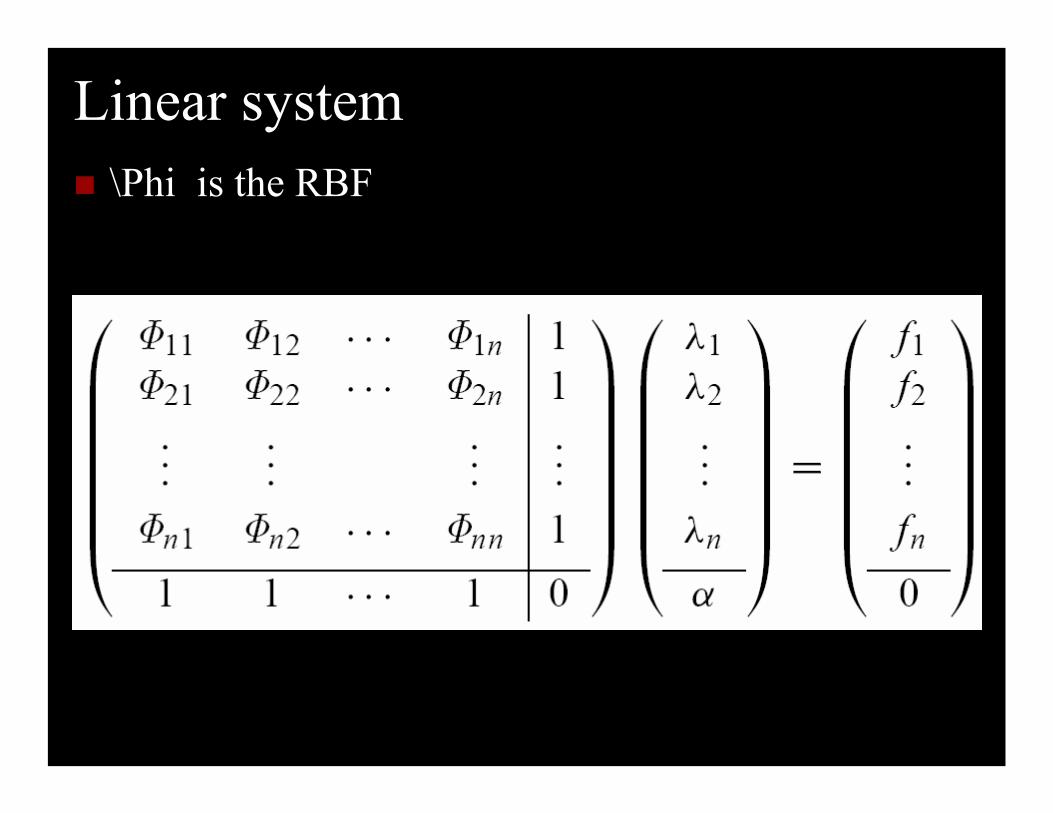
Linear system\Phi is the RBF
Preconditioner via cardinal functionsBeatson and Powell (1992) created preconditioners via approximate cardinal functionsPreconditioner must be close to the inverseCardinal function has value one at the point and zeros at all other pointsThus a cardinal function “c” satisfiesAc = [ 0 0 … 1 … 0 0]t
If we stack cardinal functions for each row, we obtain A-1 fBP92, proposed to use the smoothness of the interpolant and required the cardinality properties at each point and several other points in the domain (not the whole set)Selection of which points to include and which points to
exclude, and their influence on preconditioner performance is the subject of several subsequent papers by the groups of Powell and Beatson.
Empirical comparison of iterative methodsWe compared several strategies proposed by the authors, and found that the proposal of Faul et al. 2005, works bestFor some of the proposed strategies, for very large (106 or more points), some of the proposed preconditioners do not converge within 1000 iterations.However Faul et al.’s preconditioned iterative algorithm converges robustly within about 50 iterations.
Accelerating the Faul et al. algorithmMatrix vector product can be accelerated via the FMM (e.g., Gumerov and Duraiswami, 2006, JCP)Choice of points for the approximate cardinal functions is very particular in Faul et al.Chooses the point that is a member of the closest pair of points, and its q closest neighbors and builds an interpolantThe first point is eliminated from future considerationAlgorithm is recursively applied and a fine-to-coarse structure of the sets of approximate cardinal functions are obtainedPreconditioned Conjugate Direction algorithm is applied along the directions of these functions Search for q closest neighbors with removal of points from the set is O(N2).
Converting it to O(N log N)Use FMM data structure to build lists of closest neighborsUse heaps to develop a dynamic data structure that allows deletionsEmployed a lemma that bounds the number of closest neighbors a point can have is a fixed number that is a function of the dimensionAchieve a point selection that is O(N log N).Details in a preprint being prepared.For a 110,000 point problem, time of the preset set went down from 2445.89 seconds to 115 seconds in 3D biharmonic interpolation
Original unstructured data104502 points
RBF/FMM interpolationto regular spatial grid
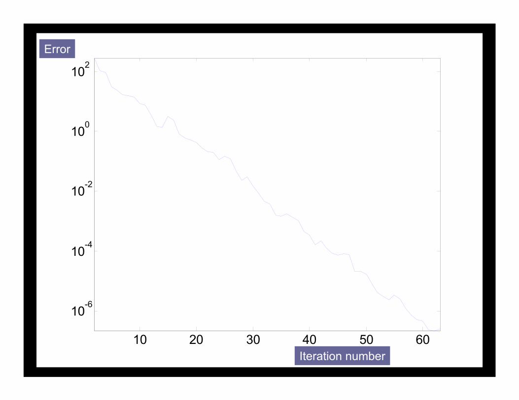
FMM algorithm cost per iteration:9.6 seconds on a Pentium IV 3.2 GHz desktop
10 20 30 40 50 60
10-6
10-4
10-2
100
102
Error
Iteration number
Original Data:
surface mesh with34834 vertices and69451 faces
RBF interpolation to the spatial grid + isosurface(size of the grid is shown near each figure)
5x5x5 11x11x11
26x26x26 51x51x51
101x101x101 201x201x201
0 100 200 300 400 5000 100 200 300 400 500
Original Image 10 percent samples drawn from image
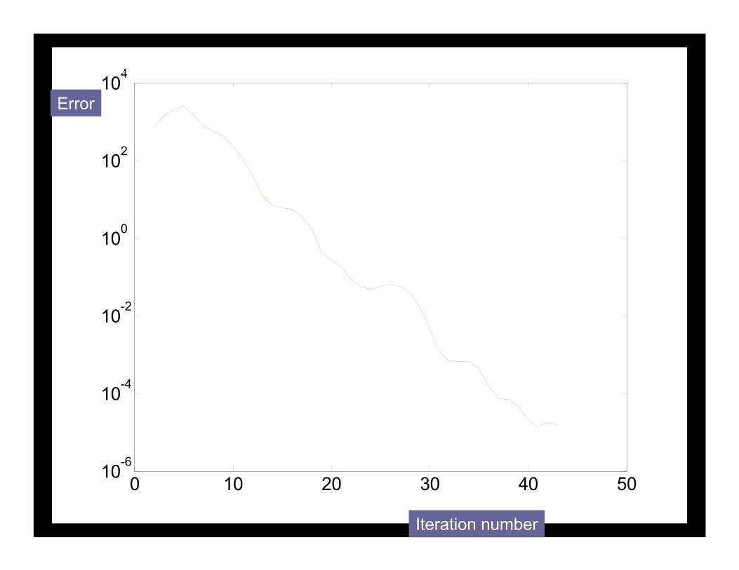
FMM algorithm cost per iteration:6.2 seconds on a Pentium IV 3.2 GHz desktop
0 10 20 30 40 5010-6
10-4
10-2
100
102
104Multiquadric Interpolation of a 2D imageError
Iteration number
0 100 200 300 00 00
Interpolated Result Difference Image
14 seconds to interpolate whole image from the fit data
Equations and Boundary Conditions
Helmholtz Equation
Impedance Boundary Conditions
Field Decomposition
Sommerfield Radiation Condition
4
2
1
6
5
3
Incident Wave
Formulation
Wave EquationFourierTransform
Scattered Field DecompositionT-Matrix Method
Expansion Coefficients
Singular Basis Functions Hankel Functions
Spherical Harmonics
Vector Form:
dot product
Scattered field expressed in terms of singular (multipole) wave functions that satisfy the Sommerfeld condition
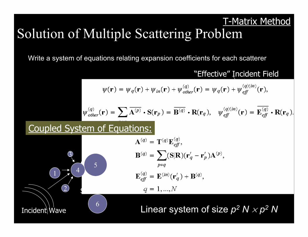
Solution of Multiple Scattering ProblemT-Matrix Method
4
2
1
6
53
Incident Wave
Scattered Wave
Coupled System of Equations:
(S|R)-TranslationMatrix
“Effective” Incident Field
Write a system of equations relating expansion coefficients for each scatterer
Linear system of size p2 N × p2 N
Three Spheres Comparisons ofBEM & MultisphereHelmholtz
T-matrix Method
BEM: 5184 triangular elementsMH: Ntrunc = 9 (100 coefficients for each sphere)
-12
-9
-6
-3
0
3
6
9
12
-180 -90 0 90 180
Angle φ1 (deg)
HR
TF (d
B)
BEMMultisphereHelmholtz
θ1 = 0o
30o
60o
90o
60o
30o
90o
120o
120o
150o
150o
180o
Three Spheres, ka1 =3.0255.
Krylov Subspace Method (GMRES)Iterative Methods
Diagonal Matrix
The product of this matrix byAn arbitrary input vector can bedone fast with the FMM
For larger systems use an iterative method
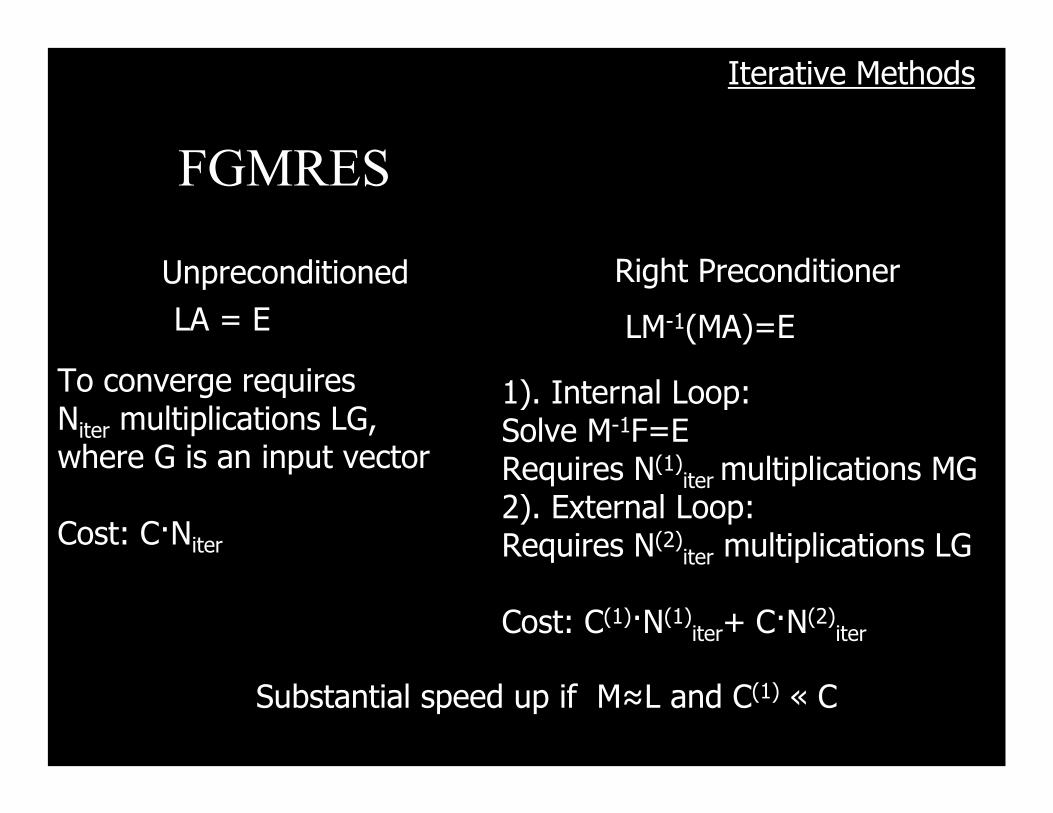
FGMRES
Iterative Methods
LA = E LM-1(MA)=E
Unpreconditioned Right Preconditioner
1). Internal Loop:Solve M-1F=ERequires N(1)
iter multiplications MG2). External Loop:Requires N(2)
iter multiplications LG
Cost: C(1)·N(1)iter+ C·N(2)
iter
To converge requiresNiter multiplications LG,where G is an input vector
Cost: C·Niter
Substantial speed up if M≈L and C(1) « C
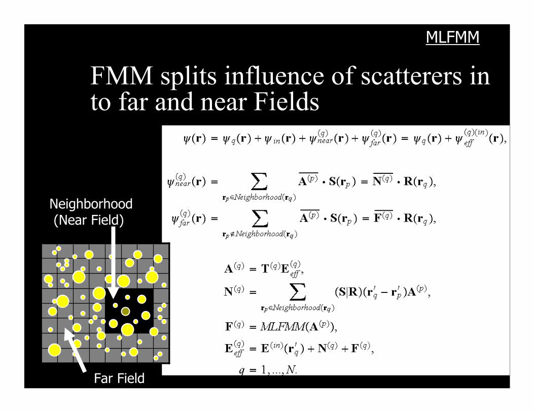
FMM splits influence of scatterers in to far and near Fields
MLFMM
Neighborhood(Near Field)
Far Field
Computation of the Far Field (1)
MLFMM
1). Set Data Structure (hierarchically subdivide space with an oct-tree)
2). multipole to multipole translate S-expansions for all scatterers in a box at the finest level to the center of the box and sum up (determine contribution to Far Field for each box at the finest level).
3). Recursively multipole to multipole translate S-expansions to center of the parent box and sum up (determine contribution to Far Field for each box at all coarser levels).
UpwardPass
(From the finestto the coarsest
level)xixc
(n,L)
y
Computation of the Far Field (2)
MLFMM
4). Multipole-to-local translate S-expansions for boxes which are inside the parent neighborhood but outside the box neighborhood to the center of the box (convert S-expansion to R-expansion).
5). Local-to-local translate R-expansions from the center of the box to the center of its children boxes (determine Far Field for each box at all levels).
DownwardPass
(From the coarsest
to the finest level)
Steps 4 and 5 performed one after the other recursively
6). local translation of R-expansions from the center of the boxes at the finest level to the centers of the spheres.
Preconditioned FGMRES FGMRES
Choice of preconditioning operator: near (sparse) or far (dense)?
Experimentally we found that the far (dense) operator works well in all tests
Range of ParametersNumber of Spheres: 1-105;ka: 0.1-50;Random and regularly spaced grids of spheres;Polydispersity: 0.5-1.5 (ratio to the mean radius);Volume fractions: 0.01-0.25
Results
100 random spheres (MLFMM)
Results
ka = 1.6
Plane Wave Plane Wave
ka = 2.8ka = 1.6
Plane Wave Plane Wave
ka = 2.8
1000 random spheres
ka=1
Results
10000 random spheres
ka = 0.75kD0 = 90
Results
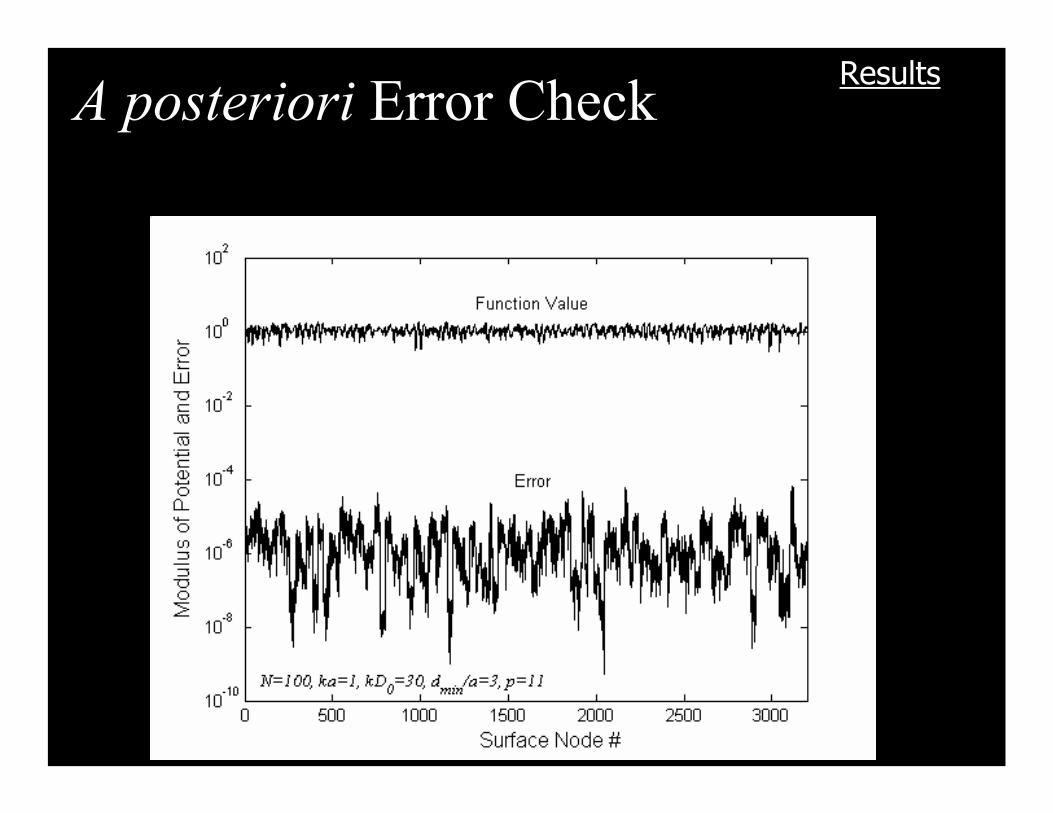
A posteriori Error Check Results
GMRES vs FGMRES
Results
Volume Fraction = 0.2ka = 0.5, D0/a = 60, p2=225
3.2GHz, Xeon,3.5 MB RAM
Performance Test Results
0.1
1
10
100
1000
10000
10 100 1000 10000
Number of Scatterers
CP
U T
ime
(s)
Total
Matrix-Vector Multiplication
External Loop
Internal Loop
y = ax
y = bx
y = cx 1.25
FMM+FGMRES
y=cx1.25
Volume fraction = 0.2,ka = 0.5, p2=225
3.2GHz, Xeon,3.5 MB RAM
ConclusionsNeed for preconditioners for dense matrices for FMM based algorithmsFor a highly oscillatory kernel, preconditioner based on the FMM algorithm itself gives good resultsPreconditioner theoretical performance remains to be provedApproach that interpolates the “cardinal” function approximately on carefully chosen data appears very promising for smoother kernelsGeometrical computations involved in this method reduced to O(N log N)
Extension to other kernels of this approach is the subject of