62
Iterative Methods Summer semester 2008 Part II of “Software for Numerical Linear Algebra” Martin H. Gutknecht ETH Zurich c Martin H. Gutknecht, 2006
Iterative Methods
Summer semester 2008
Part II of “Software for Numerical Linear Algebra”
Martin H. Gutknecht
ETH Zurich
c© Martin H. Gutknecht, 2006
Iterative Methods Contents
Contents
1 Some Basic Ideas 1-1
1.1 Sparse Matrices . . . . . . . . . . . . . . . . . . . . . . . . 1-1
1.2 Sparse Direct Methods . . . . . . . . . . . . . . . . . . . . 1-5
1.3 Fixed Point and Jacobi Iteration . . . . . . . . . . . . . . 1-6
1.4 Iterations Based on Matrix Splittings . . . . . . . . . . . . 1-10
1.5 Krylov Subspaces and Krylov Space Solvers . . . . . . . . 1-14
1.6 Chebyshev Iteration . . . . . . . . . . . . . . . . . . . . . 1-20
1.7 Preconditioning . . . . . . . . . . . . . . . . . . . . . . . . 1-26
1.8 Some Basic Preconditioning Techniques . . . . . . . . . . 1-28
1.8.1 Preconditioning based on classical matrix splittings1-28
1.8.2 Incomplete LU and Cholesky factorizations . . . . 1-29
1.8.3 Polynomial preconditioning . . . . . . . . . . . . . 1-31
1.8.4 Inner-outer iteration . . . . . . . . . . . . . . . . . 1-31
2 The Conjugate Gradient Method 2-1
2.1 Energy Norm Minimization . . . . . . . . . . . . . . . . . 2-1
2.2 Steepest Descent . . . . . . . . . . . . . . . . . . . . . . . 2-2
2.3 Conjugate Direction Methods . . . . . . . . . . . . . . . . 2-3
2.4 The Conjugate Gradient (CG) method . . . . . . . . . . . 2-5
2.5 The Conjugate Residual (CR) Method . . . . . . . . . . . 2-12
2.6 A Bound for the Convergence . . . . . . . . . . . . . . . . 2-15
2.7 Preconditioned CG Algorithms . . . . . . . . . . . . . . . 2-16
2.8 CG and CR for Complex Systems . . . . . . . . . . . . . . 2-18
2.9 CG for Least Squares Problems . . . . . . . . . . . . . . . 2-18
c©M.H. Gutknecht May 20, 2008 IM Script Contents–i
Iterative Methods Sparse Matrices
Chapter 1
Some Basic Ideas
1.1 Sparse Matrices
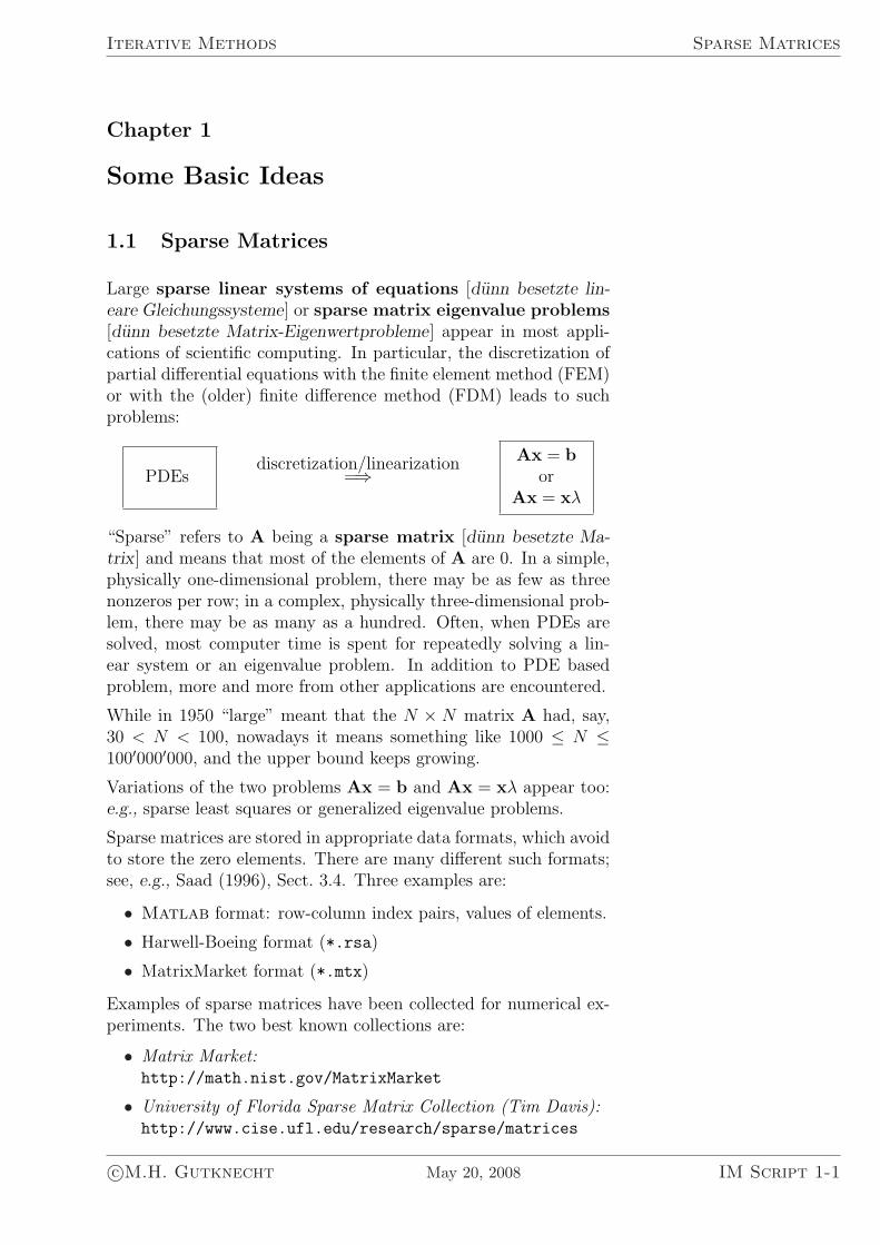
Large sparse linear systems of equations [dunn besetzte lin-eare Gleichungssysteme] or sparse matrix eigenvalue problems[dunn besetzte Matrix-Eigenwertprobleme] appear in most appli-cations of scientific computing. In particular, the discretization ofpartial differential equations with the finite element method (FEM)or with the (older) finite difference method (FDM) leads to suchproblems:
PDEsdiscretization/linearization
=⇒Ax = b
orAx = xλ
“Sparse” refers to A being a sparse matrix [dunn besetzte Ma-trix] and means that most of the elements of A are 0. In a simple,physically one-dimensional problem, there may be as few as threenonzeros per row; in a complex, physically three-dimensional prob-lem, there may be as many as a hundred. Often, when PDEs aresolved, most computer time is spent for repeatedly solving a lin-ear system or an eigenvalue problem. In addition to PDE basedproblem, more and more from other applications are encountered.
While in 1950 “large” meant that the N × N matrix A had, say,30 < N < 100, nowadays it means something like 1000 ≤ N ≤100′000′000, and the upper bound keeps growing.
Variations of the two problems Ax = b and Ax = xλ appear too:e.g., sparse least squares or generalized eigenvalue problems.
Sparse matrices are stored in appropriate data formats, which avoidto store the zero elements. There are many different such formats;see, e.g., Saad (1996), Sect. 3.4. Three examples are:
• Matlab format: row-column index pairs, values of elements.
• Harwell-Boeing format (*.rsa)
• MatrixMarket format (*.mtx)
Examples of sparse matrices have been collected for numerical ex-periments. The two best known collections are:
• Matrix Market:http://math.nist.gov/MatrixMarket
• University of Florida Sparse Matrix Collection (Tim Davis):http://www.cise.ufl.edu/research/sparse/matrices
c©M.H. Gutknecht May 20, 2008 IM Script 1-1
Some Basic Ideas Iterative Methods
Matlab provides commands that extend many operations andfunctions to sparse matrices.
• Help command: help sparfun
• Directory of m-files: matlab/toolbox/matlab/sparfun
• Examples of “sparse Matlab” commands:
sparse converts full to sparse matrixfull converts sparse to full matrixspeye sparse unit matrixspy visualizes the sparsity pattern of a sparse matrix+, -, * also applicable to sparse matrices\ , / also for solving a linear system with sparse matrix
In the iterative methods discussed here A is only needed to computeAy for any y ∈ RN (or any y ∈ CN if the matrix is complex). Thus,A may be given as a procedure/function
A : y 7→ Ay .
We will refer to this operation as a matrix-vector multiplication(MV) [Matrix-Vektor-Multiplikation], although in practice the re-quired computation may be much more complicated than multi-plying a sparse matrix with a vector; in general, Ay is just anabbreviation for finding the result of a possibly lengthy calculation(which, e.g., may include solving certain other linear systems).
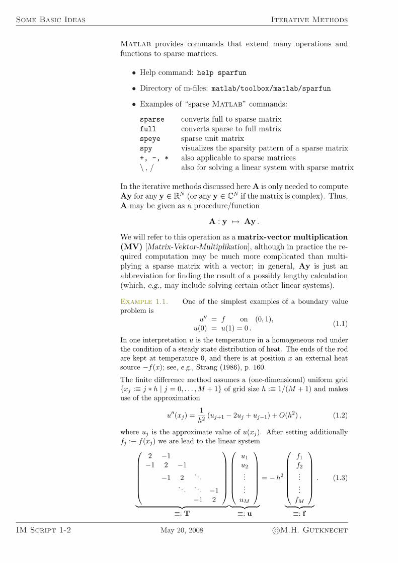
Example 1.1. One of the simplest examples of a boundary valueproblem is
u′′ = f on (0, 1),u(0) = u(1) = 0 .
(1.1)
In one interpretation u is the temperature in a homogeneous rod underthe condition of a steady state distribution of heat. The ends of the rodare kept at temperature 0, and there is at position x an external heatsource −f(x); see, e.g., Strang (1986), p. 160.
The finite difference method assumes a (one-dimensional) uniform grid{xj :≡ j ∗ h | j = 0, . . . ,M + 1} of grid size h :≡ 1/(M + 1) and makesuse of the approximation
u′′(xj) =1h2
(uj+1 − 2uj + uj−1) + O(h2) , (1.2)
where uj is the approximate value of u(xj). After setting additionallyfj :≡ f(xj) we are lead to the linear system
2 −1−1 2 −1
−1 2. . .
. . . . . . −1−1 2
︸ ︷︷ ︸≡: T
u1
u2......
uM
︸ ︷︷ ︸≡: u
= −h2
f1
f2......
fM
︸ ︷︷ ︸≡: f
. (1.3)
IM Script 1-2 May 20, 2008 c©M.H. Gutknecht
Iterative Methods Sparse Matrices
Here the M ×M system matrix T is symmetric tridiagonal and can beseen to be positive definite. (It is weakly diagonally dominant.) Thesystem could be solved easily by Gaussian elimination, that is by LUfactorization, by LDLT factorization, or by Cholesky factorization. Thecost of such a factorization is only O(M) since the factors are bidiagonal.There exist yet other efficient recursive algorithms for solving such asystem, for example, cyclic reduction or fast Toeplitz solvers, since Thas also Toeplitz structure (i.e., tij only depends on i− j).
The corresponding two-dimensional example is the Poisson problem
∆u = f on S :≡ (0, 1)× (0, 1) ,u(x, y) = 0 on ∂S ,
(1.4)
where
∆u :≡ ∂2u
∂x2+
∂2u
∂y2.
Here ∂S denotes the boundary of the unit square S. In analogy to (1.2)we apply the approximation
∆u(xj , yj) =1h2
[(uj+1 − 2uj + uj−1) + (uj+M − 2uj + uj−M )]+O(h2) ,
(1.5)where we assume that the N :≡ M2 interior points are numbered row byrow from the upper left corner to the lower right one. This transforms(1.4) into the linear system
Au = −h2f (1.6)
with the block matrix A of size N ×N = M2 ×M2 defined by
A :≡
T −I O · · · · · · O
−I T −I. . .
...
O −I T. . . . . .
......
. . . . . . . . . −I O...
. . . −I T −I
O · · · · · · O −I T
. (1.7)
Here, I is the M ×M unit matrix and
T :≡
4 −1−1 4 −1
−1 4. . .
. . . . . . −1−1 4
is also of size M ×M . The system matrix A is still symmetric positivedefinite and banded, but the total bandwidth is now 2M +1. Clearly, inthree dimensions we would have N = M3 and obtain a matrix with totalbandwidth 2M2 + 1 and with at most seven nonzeros per row, namelyone number six and at most six minus ones.
Note that the matrices depend on the numbering or order of the points.For example, if in the first problem (1.3) we take all the currently odd
c©M.H. Gutknecht May 20, 2008 IM Script 1-3
Some Basic Ideas Iterative Methods
numbered points first, followed by all even numbered points — a one-dimensional version of what is called red-black ordering — the matrixT is transformed into
T :≡(
2 I −B1
−BT1 2 I
), (1.8)
where B1 is a lower bidiagonal matrix of ones of size 12M if M is even.
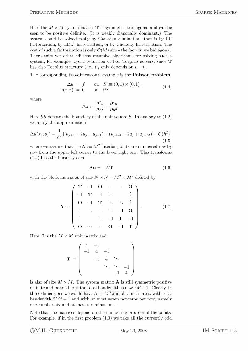
Likewise, by using red-black ordering in the two-dimensional problem(1.6) and assuming M odd we can replace A by
A :≡(
4I1 −B2
−BT2 4I2
), (1.9)
where I1 is the unit matrix of size1 d12M2e and I2 is the unit matrix
of size b12M2c, while B2 is a (non-square) Toeplitz matrices with four
co-diagonals of ones (but not all next to each other). The nonzeros ofA are shown in the following “spy plot” (with M = 9, N = 81):
0 10 20 30 40 50 60 70 80
0
10
20
30
40
50
60
70
80
nz = 369
It was generated with the following Matlab commands:
M = 9; N = M2;A = gallery(′poisson′,M);p = [1 : 2 : N, 2 : 2 : N ];Atilde = A(p, p);spy(Atilde) ¨
In most applications the data are real, i.e., A ∈ RN×N and b ∈ RN .But, e.g., in electrical engineering there are also problems whereA ∈ CN×N and b ∈ CN . Most of what we say is true for both cases.To handle them at once we will write A ∈ EN×N , b ∈ EN withE :≡ R or C, and use x? :≡ xT if E = R and x? :≡ xH if E = C.
Except in the sections on least squares we will assume that A isnonsingular. In many applications A is real symmetric or Hermitianand positive definite (or, briefer: spd or Hpd) — in which case allthe eigenvalues are positive, and there is an orthonormal basis ofeigenvectors. We will see that solving the linear system Ax = b isthen much easier than when A is indefinite or even nonsymmetric.
1dye denotes the smallest integer larger or equal to y, and byc denotes thelargest integer smaller or equal to y.
IM Script 1-4 May 20, 2008 c©M.H. Gutknecht
Iterative Methods Sparse Direct Methods
1.2 Sparse Direct Methods
In connection with the solution of sparse linear systems the term“direct method” is used for all methods that are in a wide sensevariations of Gaussian elimination or — what is essentially the same— LU decomposition (or LU factorization) :
PA = LU .
Here, P is a permutation matrix representing possible row inter-changes, and the matrices L and U are lower and upper triangular,respectively.
The cost of such a decomposition is roughly
∼ 23N3 flops in general
∼ 2b2N flops if A banded, bandwidth b ¿ N
reduced by ∼ 50% if A sym. pos. def.
These variations of Gauss elimination for sparse linear systems arecalled sparse direct methods or sparse direct solvers. But themore A differs from a narrowly banded matrix, the less effectivethey are due to fill-in: the matrix L + R may contain many morenonzeros than A.
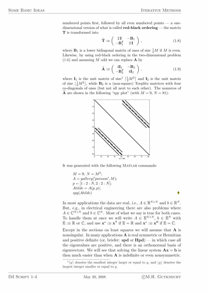
If the original physical problem is 2- or 3-dimensional, A will be farfrom being narrowly banded. For example, the Cholesky factors ofthe matrices A and A of the previous section have the followingnonzero patterns:
0 20 40 60 80
0
10
20
30
40
50
60
70
80
nz = 7370 20 40 60 80
0
10
20
30
40
50
60
70
80
nz = 531
The ordering of equations and unknowns effects the fill-in, and canbe used to reduce it. There exist several well established algorithmsto achieve this. But pivoting complicates matters further.
In the last twenty years enormous effort has been spent for vector-izing and parallelizing sparse direct solvers; see, e.g., the programPARDISO by Schenk (2000).
Also in Matlab a sparse direct solver is implemented. It is calledwhenever a linear system Ax = b or wTA = cT with a sparsematrix A is solved by writing x = A\b or w’ = c’/A, respectively.
Freely available software for sparse direct solvers and for some otherlinear algebra tasks can be found on
http://www.netlib.org/utk/people/JackDongarra/la-sw.html
c©M.H. Gutknecht May 20, 2008 IM Script 1-5
Some Basic Ideas Iterative Methods
1.3 Fixed Point and Jacobi Iteration
Pure mathematicians often write nonlinear equations in fixed pointform as x = Φ(x), and solve them under the assumption that Φis a contraction by the so-called Picard iteration or fixed pointiteration [Fixpunkt-Iteration] xn+1 := Φ(xn). This idea is alsoapplicable to a linear system Ax = b: we rewrite it in fixed pointform as
x = Bx + b with B :≡ I−A (1.10)
and apply fixed point iteration: starting with some x0, we computefor n = 0, 1, 2, . . .
xn+1 := Bxn + b . (1.11)
Here, xn is the nth approximation of the fixed point x? satisfyingx? = Bx? +b, i.e., Ax? = b; it is also called nth iterate [Iterierte].
If ak,k = 1 (∀k), i.e., bk,k = 0 (∀k), then iteration (1.11) is calledJacobi iteration [Gesamtschritt-Verfahren]. Note that ak,k = 1can be achieved whenever ak,k 6= 0 by scaling the kth equation.
In the linear case, Φ : x 7→ Bx is called a contraction [Kon-traktion] if ‖B‖ < 1 in some norm. Then the linear fixed pointiteration converges globally, that is, for every x0. The proof is leftas an easy exercise. But we can establish a sharper result becausethe underlying space is finite dimensional:
Theorem 1.3.1 For the (linear) fixed point iteration (1.11) holds
xn → x? for any x0 ⇐⇒ ρ(B) < 1 , (1.12)
where ρ(B) :≡ max{|λ|∣∣ λ eigenvalue of B} is the spectral ra-
dius of B.
Proof. Let BV = VΛ be an eigenvalue decomposition of B, so thatΛ is diagonal or, in general, the Jordan canonical form [JordanscheNormalform] of B. Clearly,
xn − x? = B(xn−1 − x?) = Bn(x0 − x?) ,
so convergence occurs if and only if Bn → O as n →∞. This, in turn,happens if and only if Λn → O as n →∞.
If Λ is diagonal, the equivalence (1.12) clearly follows. But in general,Λ is block diagonal and may contain bidiagonal Jordan blocks [Jor-dansche Blocke] like
Jk :≡
λk 1 0 · · · 0
0 λk 1. . .
......
. . . . . . . . . 0...
. . . λk 10 · · · · · · 0 λk
. (1.13)
IM Script 1-6 May 20, 2008 c©M.H. Gutknecht
Iterative Methods Fixed Point and Jacobi Iteration
It remains to show that Jnk → O as n → ∞. Assume Jk is of size
mk ×mk. We write it as Jk = λkI + S and note that S` is zero exceptfor ones on the `th upper codiagonal. In particular, S` = O when` ≥ mk. Therefore, if n ≥ mk − 1,
Jnk = (λkI + S)n =
n∑
i=0
(n
i
)λn−i
k Si =mk−1∑
i=0
(n
i
)λn−i
k Si . (1.14)
In this finite sum, in view of |λk| < 1, in each term we have, as n →∞,(
n
i
)λn−i
k =n(n− 1) · (n− i + 1)
i!λn−i
k → 0 .
Consequently, Jnk → O as n →∞. ¤
Remark. A matrix norm is called compatible [kompatibel] witha given vector norm if ‖By‖ ≤ ‖B‖ ‖y‖ for any square matrix Band any vector y of matching size. For a compatible matrix normwe have ‖B‖ ≥ ρ(B) as is seen by choosing for y an eigenvectorcorresponding to an eigenvalue of largest absolute value, so that‖By‖ = ρ(B) ‖y‖. So, ρ(B) < 1 if ‖B‖ < 1 for some norm. H
Theorem 1.3.1 can be recast as follows: linear fixed point iterationin EN is globally convergent if and only if ρ(B) < 1. By a carefulanalysis of its proof we can also specify the speed of convergence2.
What can we say about the rate of convergence?
Theorem 1.3.2 If ρ(B) < 1 then, for any x0, the iterates of thelinear fixed point iteration (1.11) satisfy
lim supn→∞
‖xn − x?‖1/n ≤ ρ(B) , (1.15)
and for some x0 equality holds.So, if 0 < ρ(B) < 1, linear fixed point iteration converges linearlywith a root-convergence factor of at most ρ(B), while if ρ(B) = 0,it converges superlinearly.
Proof. We have, as in the proof of Theorem 1.3.1,
‖xn − x?‖1/n = ‖VΛnV−1(x0 − x?)‖1/n ≤ ‖V‖1/n‖Λnw0‖1/n ,
where w0 :≡ V−1(x0 − x?). Since ‖V‖1/n → 1, all depends on Λn,whose diagonal blocks are eigenvalues or Jordan blocks Jk. The powers
2A sequence {xn} ⊂ CN is said to converge R-linearly to x? if the R-factoror root-convergence factor [Wurzel-Konvergenzfaktor]
κR{xn} :≡ lim supn→∞
‖xn − x?‖1/n
lies in (0, 1). An iterative process J that generates a nonempty set C(J ,x?)of sequences that converge R-linearly to the limit point x? has R-factor
κR(J ) :≡ sup {R{xn} | {xn} ∈ C(J ,x?)} .
c©M.H. Gutknecht May 20, 2008 IM Script 1-7
Some Basic Ideas Iterative Methods
of the latter were considered in (1.14). If we write, with ρ :≡ ρ(B),
Jnk = ρn
mk−1∑
i=0
(n
i
)λ−i
k
(λk
ρ
)n
Si , (1.16)
it is evident that only eigenvalues of maximum absolute value count,because for the others the nth power of the fraction λk/ρ tends to zero.If |λk| = ρ, the dominant term in the sum (1.16) is
(n
mk − 1
)λn−mk+1
k Smk−1 .
There may be several such terms. In any case, ‖Λnw0‖1/n behavesasymptotically at worst like the nth root of the absolute value of sucha term, hence like |λk| = ρ. So this is asymptotically a bound for‖xn−x?‖1/n. To see that this bound is sharp we just have to choose x0
so that w0 is an eigenvector of Λ for a dominant eigenvalue λk. ¤
The applicability of fixed point or Jacobi iteration in practice isquite limited since, if ρ(B) < 1 holds at all, then typically onlywith ρ(B) nearly 1, so that convergence is very slow. But we needa good approximate solution in n ¿ N steps.
Example 1.2. We continue Example 1.1: it can be seen that theM ×M matrix T in (1.3) has the eigenvalues
λj = 2− 2 cosjπ
M + 1= 4 sin2 jπ
2(M + 1)= 4 sin2 hjπ
2.
Thus, when we divide every equation by 2, so that ak,k = 12 tk,k = 1 and
bk,k = 1− ak,k = 0, then
ρ(B) = ρ(I− 12T) = cos
π
M + 1= coshπ . (1.17)
For example, when M = 100, then ρ(B) = 0.9995 1628...
In order to reduce the error by a factor of 10, we need 4760 iterations!
It helps to use a courser grid: for M = 10 we have ρ(B) = 0.9594 9297..,and “only” 56 iterations are needed to reduce the error by a factor of10, but of course this is still excessive for a 10× 10 system.
To verify (1.17) with Matlab, B and its spectral radius can be foundby
B = gallery(′tridiag′,M, 0.5, 0, 0.5);rhoB = norm(full(B))
or better by
B = gallery(′tridiag′,M, 0.5, 0, 0.5);svd6 = svds(B); rhoB = svd6(1)
¨
IM Script 1-8 May 20, 2008 c©M.H. Gutknecht
Iterative Methods Fixed Point and Jacobi Iteration
Since we cannot compute the nth error (vector) [Fehler(vektor)]
dn :≡ xn − x? (1.18)
for checking the convergence of an iteration, i.e., for checking the“quality” of the approximate solution (or, iterate) xn, we use thenth residual (vector) [Residuum, Residuenvektor]
rn :≡ b−Axn . (1.19)
Note thatrn = −A(xn − x?) = −Adn . (1.20)
For the linear fixed point iteration we have
rn = b−Axn = Bxn + b− xn = xn+1 − xn ,
so we can rewrite it as
xn+1 := xn + rn , (1.21)
and, by multiplying it by−A, we obtain a recursion for the residual,
rn+1 := rn −Arn = Brn . (1.22)
We see that we can compute the residual rn either according to thedefinition (1.19) or by using the recursion (1.22). In either case,we need one matrix-vector multiplication. Once, rn is known, thenew iterate xn+1 is obtained without any matrix-vector multiplica-tion from (1.21). Mathematically both ways of computing rn areequivalent, but roundoff errors may cause the results to differ.
Assignment (1.21) is a typical update formula for the iterate: thenew approximation of the solution is obtained by adding a correc-tion, here rn, to the old one.
From (1.22) it follows by induction that
rn = pn(A)r0 ∈ span {r0,Ar0, . . . ,Anr0} , (1.23)
where pn is a polynomial of exact degree n, actually pn(ζ) = (1−ζ)n.Moreover, from (1.21) we conclude that
xn = x0 + r0 + · · ·+ rn−1 (1.24a)
= x0 + qn−1(A)r0 (1.24b)
∈ x0 + span{r0,Ar0, . . . ,A
n−1r0
}(1.24c)
with a polynomial qn−1 of exact degree n−1. We note that here x0+span {r0,Ar0, . . . ,A
n−1r0} is an affine space, i.e., a linear subspaceshifted by the translation x0.
Building up xn = x0 + qn−1(A)r0 and rn = pn(A)r0 requires inparticular a total of n + 1 matrix-vector multiplications and this isthe main work of the whole iteration process (unless A is extremelysparse). With roughly the same work we can construct any othervector xn in the same affine space and its corresponding residual.We may hope that by making a better choice in this space we willfind a sequence (xn) that converges faster.
c©M.H. Gutknecht May 20, 2008 IM Script 1-9
Some Basic Ideas Iterative Methods
1.4 Iterations Based on Matrix Splittings
We introduced the Jacobi iteration as fixed point iteration (1.11)with a matrix B whose diagonal elements are zero. If we start froman arbitrary nonsingular system Ax = b and let D be the diagonalmatrix with the diagonal of A, we thus replace the system by
x = Bx + b with B :≡ I−D−1A , b :≡ D−1b (1.25)
and apply the fixed point iteration xn+1 := Bxn + b.
Written in terms of the components of xn ≡:(
x(n)1 . . . x
(n)N
)T
one step — or, as it is often called, one sweep — of Jacobi iterationbecomes
x(n+1)j :=
1
ajj
(bj −
j−1∑
k=1
ajk x(n)k −
N∑
k=j+1
ajk x(n)k
), j = 1, . . . , N .
(1.26)It seems that Gauss was the one who discovered that the conver-gence is usually improved if we replace in the first sum of (1.26)
the old values x(k)n by the already computed new values x
(k)n+1:
x(n+1)j :=
1
ajj
(bj −
j−1∑
k=1
ajk x(n+1)k −
N∑
k=j+1
ajk x(n)k
), j = 1, . . . , N .
(1.27)This is called Gauss-Seidel method [Gauss-Seidel-Verfahren oderEinzelschrittverfahren]. To recast it in matrix notation we write Aas
A = D− E− F , (1.28)
where E and F are strictly lower and upper triangular, respectively.Then (1.27) becomes
Dxn+1 := Exn+1 + Fxn + b
or(D− E)xn+1 := Fxn + b , (1.29)
which can be brought into the form of fixed point iteration with
B :≡ (D− E)−1F , b :≡ (D− E)−1b . (1.30)
Of course, we never intend to compute the lower triangular matrix(D− E)−1, but implement this recursion as the sweep (1.27). Therepresentation as fixed point iteration tells us that for a convergenceanalysis we have to determine the spectral radius of B.
In the notation (1.28) Jacobi iteration takes the form
xn+1 := D−1(E + F)xn + D−1b = xn + D−1rn (1.31)
IM Script 1-10 May 20, 2008 c©M.H. Gutknecht
Iterative Methods Iterations Based on Matrix Splittings
and has the iteration matrix
B :≡ D−1(E + F) . (1.32)
A classical idea is to apply here is that of relaxation [Relaxation]:we multiply the correction D−1rn in the Jacobi iteration (1.31) by arelaxation factor [Relaxationsfaktor] ω, which typically satisfies0 < ω < 1:
xn+1 := xn + D−1rnω . (1.33)
Naturally this method is called the damped Jacobi iteration[gedampftes Gesamtschritt-Verfahren]. It has also been referredto as Jacobi overrelaxation (JOR) method or as stationaryRichardson iteration. (In general, Richardson iteration is non-stationary, that is, ω :≡ ωn depends on n.)
Note that
xn+1 = xn + D−1 [b−Axn] ω
= xn(1− ω) + D−1 [(E + F)xn + b] ω
= xn(1− ω) + xJacn+1ω . (1.34)
So the new iterate xn+1 is the weighted mean of the old iterate xn
and one step of Jacobi, (1.31), starting from xn.
The iteration matrix is now
B :≡ (1− ω)I + ωD−1(E + F) = I− ωD−1A . (1.35)
If the spectrum of D−1A lies, e.g., on the interval [α, β] of the
positive real axis, the one of B lies on [1− ωβ, 1− ωα]. Therefore,if ω > 0 is chosen such that ωβ < 2, we will have convergence(according to Theorem 1.3.1). Moreover, ω could be chosen easilysuch that max{|1−ωβ|, |1−ωα|} is minimal, and thus ω is optimal.
It was Young (1950) who realized in his dissertation that the ideaof relaxation is particularly effective in connection with the Gauss-Seidel method: we take componentwise a weighted mean of the olditerate x
(j)n and a step of Gauss-Seidel for that component, as given
by (1.27):
x(n+1)j := x
(n)j (1− ω) + x
(n+1,GS)j ω (1.36)
= x(n)j (1− ω) +
ω
ajj
(bj −
j−1∑
k=1
ajk x(n+1)k −
N∑
k=j+1
ajk x(n)k
),
j = 1, . . . , N .
This translates into
(D− ωE)xn+1 := [(1− ω)D + ωF]xn + ωb (1.37)
c©M.H. Gutknecht May 20, 2008 IM Script 1-11
Some Basic Ideas Iterative Methods
or the fixed point iteration with
B :≡ (1ωD− E
)−1 [(1ω− 1
)D + F
], b :≡ (
1ωD− E
)−1b
(1.38)and is called successive overrelaxation (SOR) method [Ver-fahren der sukzessiven Uberrelaxation]. It can be shown that forfixed ω in the interval 0 < ω < 2 the method converges for any sys-tem with Hpd matrix A. (For a proof, see, e.g., p. 56 of Schwarz,Rutishauser and Stiefel (1968).)
There remains the question on how to choose ω so that convergenceis fastest. Young (1950) derived a beautiful theory leading to theoptimal ω for matrices that have the so-called Property A and areconsistently ordered [konsistent geordnet]. The class of matriceswith Property A includes many examples obtained by discretizingpartial differential equations with the finite difference method. Theproperty is (by definition) invariant under simultaneous column androw permutations of the matrix, but for optimal convergence weneed rows and columns so-called consistently ordered.
For example, the matrix A of (1.7) has Property A, but only Aof (1.9) is also consistently ordered. Although we do not exactlydefine Property A and consistent ordering here, we give a statementof Young’s convergence result. For partial proofs under slightlyvarying assumptions see, e.g., pages 59–65 and 208–211 of Schwarzet al. (1968) (for A spd), pages 112–116 of Saad (1996) (discussionof consistent ordering, but no proof of optimal ω), and pages 149–154 of Greenbaum (1997) (no discussion of consistent ordering).
Theorem 1.4.1 For a consistently ordered matrix A with Prop-erty A and real eigenvalues of D−1A, the optimal relaxation fac-tor ωopt of the SOR method is
ωopt :≡ 2
1 +√
1− λ2max
, (1.39)
where, in terms of notation (1.28), λmax is the largest eigenvalueof the matrix D−1(E + F), which is the iteration matrix of theJacobi method. The spectral radius of the optimal SOR iterationmatrix Bopt is then
ρ(Bopt) = ωopt − 1 , (1.40)
An interesting aspect is that, under the assumptions of the theorem,the real eigenvalues of D−1A are mapped by SOR with optimal ωonto the circle with radius ρ(Bopt). So all the eigenvalues of Bopt,although in general complex, have the same absolute value.
A further related method is the symmetric SOR (SSOR)method, where each step is a double step consisting of an SORstep followed by a backward SOR step; in short form:
IM Script 1-12 May 20, 2008 c©M.H. Gutknecht
Iterative Methods Iterations Based on Matrix Splittings
(D− ωE)xn+ 12
:= [(1− ω)D + ωF]xn + ωb ,
(D− ωF)xn+1 := [(1− ω)D + ωE]xn+ 12
+ ωb .(1.41)
The convergence analysis is even more complicated than for SOR.
There are also block versions of all these schemes. For example, onemay consider the equations and the unknowns that belong to pointson a line of the discretized Poisson equation (1.6) as a group defininga diagonal block of A. Then, in (1.28), D will be a block diagonalmatrix and E, F the corresponding block triangular parts. Withthis new meaning for D, E, and F, the various methods discussedin this section can be redefined.
Except for SSOR all the methods discussed in this section can beviewed as applications of the general principle of improving fixedpoint iteration by matrix splitting: we write
A = M−N , (1.42)
where M is chosen so that, for any y, the system Mx = y is easyto solve for x. Then an iterative method can be defined by
Mxn+1 := Nxn + b = Mxn + rn . (1.43)
In every step a linear system with the matrix M has to be solved.Formally, the method is equivalent with
xn+1 := M−1Nxn + M−1b = xn + M−1rn . (1.44)
This is just a linear fixed point iteration with
B :≡ M−1N , b :≡ M−1b . (1.45)
Therefore, the iteration converges if and only if ρ(M−1N) < 1. So,the aim must be to find splittings (1.42) where this spectral ra-dius is small. Unfortunately, in general it is difficult to concludefrom the spectrum of A on that of B = M−1N. But there is theimportant class of so-called M-matrices [M-Matrizen] and corre-sponding so-called regular splittings [regulare Splittings] whereat least convergence can be proved.
Table 1.1 summarizes the meanings of M and N in our abovetreated classical methods. These methods, in particular SOR, werevery popular in the 1950ies and 1960ies, but they are hardly usednowadays for the original purpose. We will come back to them inSection 1.8 on basic preconditioning techniques, however.
c©M.H. Gutknecht May 20, 2008 IM Script 1-13
Some Basic Ideas Iterative Methods
Table 1.1 Some matrix splittings based on A = D− E− F.
method M N
Jacobi D E + FGauss-Seidel D− E Fdamped Jacobi 1
ωD
(1ω− 1
)D + E + F
SOR 1ωD− E
(1ω− 1
)D + F
backward SOR 1ωD− F
(1ω− 1
)D + E
1.5 Krylov Subspaces and Krylov Space Solvers
The discussion of the Jacobi method in Section 1.3 suggests to lookfor better approximate solutions lying in the following affine space:
xn ∈ x0 + span{r0,Ar0, . . . ,A
n−1r0
},
see (1.24c). We first investigate the subspace that appears in thisformula.
Definition. Given a nonsingular N × N matrix A and anN -vector y 6= o, the nth Krylov (sub)space Kn(A,y) [Krylov–Raum] generated by A from y is
Kn :≡ Kn(A,y) :≡ span (y,Ay, . . . ,An−1y). (1.46)
N
Clearly, by this definition, whenever z ∈ Kn(A,y), there is a poly-nomial p of degree at most n− 1 such that z = p(A)y. In general,this polynomial may be not unique since the spanning set in (1.46)may be linearly dependent. We can say more about this in a mo-ment.
Definition (1.46) associates with a matrix A and a starting vectory a whole nested sequence of Krylov subspaces:
K1 ⊆ K2 ⊆ K3 ⊆ ... .
The following lemma answers the question of the equality signs.
Lemma 1.5.1 There is a positive integer ν :≡ ν(y,A) such that
dim Kn(A,y) =
{n if n ≤ ν ,ν if n ≥ ν .
The inequalities 1 ≤ ν ≤ N hold, and ν < N is possible if N > 1.
Definition. The positive integer ν :≡ ν(y,A) of Lemma 1.5.1is called grade of y with respect to A [Grad von y bezuglichA]. N
Proof of Lemma 1.5.1. By definition (1.46),
Kn :≡ Kn(A,y) :≡ span (y,Ay, . . . ,An−1y) ,
IM Script 1-14 May 20, 2008 c©M.H. Gutknecht
Iterative Methods Krylov Subspaces and Krylov Space Solvers
with some y 6= o. So, dimK1 = 1, and if y,Ay, . . . ,An−1y are linearlyindependent, then dimKn = n. Let n = ν be the first n for whichy,Ay, . . . ,An−1y,Any are linearly dependent. Then Any = Aνy is alinear combination of the linearly independent vectors y,Ay, . . . ,Aν−1y:
Aνy = yγ0 + Ayγ1 + · · ·+ Aν−1yγν−1 . (1.47)
Here, γ0 6= 0, because otherwise, after multiplication by A−1, we wouldhave
Aν−1y = yγ1 + Ayγ2 + · · ·+ Aν−2yγν−1 ,
in contrast to the assumption that the vectors on the right-hand sideare linearly independent.
If we consider the definition (1.46) for some n > ν, then, by using (1.47),all terms Aky with k ≥ ν in the span can be recursively replaced bysums of terms with k < ν. So, the dimension cannot be larger than ν;and of course, it cannot be smaller since Kn ⊇ Kν if n ≥ ν.
If we choose y as an eigenvector of A, then ν = 1, so ν can be smallerthan N if N > 1. ¤
We can say more and understand the structure of the Krylov sub-spaces better if we consider the Jordan canonical form of A (as inthe proof if Theorem 1.3.1) and recall the notion of the minimalpolynomial of A. So we let A = VΛV−1 be the Jordan decompo-sition of A, i.e., Λ is a block-diagonal matrix of the form
Λ =
J1
. . .
Jµ
, where Jk =
λk 1
λk. . .. . . 1
λk
∈ Cmk×mk
(1.48)are either bidiagonal Jordan blocks or 1×1 blocks (λk). Some of theeigenvalues λk in the different blocks may coincide, and we choose torearrange the blocks so that a full set of Jordan blocks of maximumsize mk corresponding to all the µ distinct eigenvalues λ1, . . . , λµ isat the top. So, if µ < µ, then λµ+1, . . . , λµ all coincide with someeigenvalue among the first µ, and the block sizes mk for k > µ areat most as large as the corresponding ones for the same eigenvaluewith k ≤ µ. Then the minimal polynomial [Minimalpolynom]χA of A is defined by
χA(t) :≡µ∏
k=1
(t− λk)mk . (1.49)
It is a divisor of the characteristic polynomial
χA(t) :≡µ∏
k=1
(t− λk)mk (1.50)
c©M.H. Gutknecht May 20, 2008 IM Script 1-15
Some Basic Ideas Iterative Methods
(where the product runs now over all µ diagonal blocks Jk of theJordan decomposition (1.48)). Its degree M :≡ ∂χA satisfies
M :≡ ∂χA =
µ∑
k=1
mk ≤µ∑
k=1
mk = ∂ψ = N .
We claim that if we insert t := A into the minimal polynomial (sothat it becomes a matrix polynomial), we get the zero matrix.
Theorem 1.5.2 If χA denotes the minimal polynomial of A,then
χA(A) =
µ∏
k=1
(A− λkI)mk = O . (1.51)
Proof. We have
χA(A) = V χA(Λ)V−1 = V
(µ∏
k=1
(Λ− λkI)mk
)V−1 ,
and here all the factors of the product, and hence the product itself,is block diagonal. Consider, the block (Jk − λkI)mk of the kth factor.In the notation of (1.14) it equals Smk , where, in this factor, S is themk×mk matrix with ones on the upper bidiagonal and zeros elsewhere.So, Smk = O. Hence, in the product in question, there is for each k afactor where the kth block is zero. Consequently, the whole product isa zero matrix, and thus also χA(Λ) and χA(A). ¤
Since the minimal polynomial is a divisor of the characteristic poly-nomial, the following famous Caley-Hamilton theorem followsimmediately.
Corollary 1.5.3 If χA denotes the characteristic polynomial ofA, then χA(A) = O.
Now we are ready to prove the following result on the grade ν thatappeared in Lemma 1.5.1.
Lemma 1.5.4 The nonnegative integer ν of Lemma 1.5.1 satisfies
ν = min{n
∣∣ A−1y ∈ Kn(A,y)} ≤ ∂χA,
where ∂χA denotes the degree of the minimal polynomial of A.
Proof. Multiplying (1.47) by A−1 we see that
A−1y =(Aν−1y −Aν−2yγν−1 − · · · −Ayγ2 − yγ1
) 1γ0
, (1.52)
so A−1y ∈ Kν(A,y). We cannot replace ν by some n < ν here, becausethis would lead to a contradiction to the minimality of ν in (1.47).
It remains to show that ν ≤ ∂χA. The product formula for χA(A) = Oin (1.51) could be written as a linear combination of I, A, . . . , AM thatis zero, but the coefficient of AM is 1 (here, again, M :≡ ∂χA). This
IM Script 1-16 May 20, 2008 c©M.H. Gutknecht
Iterative Methods Krylov Subspaces and Krylov Space Solvers
remains valid if we post-multiply each term by any y. So, for any y, theKrylov subspace KM+1(A,y) has dimension at most M , and in view ofLemma 1.5.1 the same is true for Kn(A,y) for any n. ¤
Of course, the actual dimension may be smaller for some y. Infact, it is, if in the representation of y in terms of the basis asso-ciated with the Jordan decomposition of A some of the relevantcoordinates vanish.
We can conclude that as long as n ≤ ν(y,A), the vectors y, Ay,. . . , An−1y in (1.46) are linearly independent, and thus the poly-nomial p representing some z = p(A)y ∈ Kn(A,y) is uniquelydetermined. In other words, as long as n ≤ ν, there is a naturalone-to-one correspondence (actually, an isomorphism) between thelinear space Kn and the linear space Pn−1 of polynomials of degreeat most n− 1.
Unfortunately, even for n ≤ ν the vectors y, Ay, . . . , An−1y formtypically a very ill-conditioned basis for Kn, since they tend to benearly linearly dependent. In fact, one can easily show that if A hasa unique eigenvalue of largest absolute value and of algebraic multi-plicity one, and if y is not orthogonal to a corresponding normalizedeigenvector v, then Aky/‖Aky‖ → ±v as k → ∞. Therefore, inpractice, we will never make use of this so-called Krylov basis[Krylovbasis].
In connection with the iterative solution of a linear systemLemma 1.5.4 yields a most welcome corollary.
Corollary 1.5.5 Let x? be the solution of Ax = b and let x0
be any initial approximation of it and r0 :≡ b − Ax0 the corre-sponding residual. Moreover, let ν :≡ ν(r0,A). Then
x? ∈ x0 +Kν(A, r0) .
Proof. By (1.18), (1.20), and by Lemma 1.5.4,
x? − x0 = d0 = −A−1r0 ∈ Kν(A, r0) .¤
This corollary shows that if we choose xn from the affine spacex0 + Kn(A, r0) there is a chance that we find the exact solutionwithin at most ν steps. We say then that our method has thefinite termination property. We will see that it is easy to deducemethods that have this property. In fact, it suffices to insure thatthe residuals rn are linearly independent as long as they are nonzero.Of course, once rn = o for some n, the linear system is solved.
However, in practice the finite termination property is normallynot important, since ν is typically much larger than the maximumnumber of iterations we are willing to execute. We rather want anapproximation with sufficiently small residual quickly.
The corollary and the analogy to the relation (1.24c) now motivatethe following definition.
c©M.H. Gutknecht May 20, 2008 IM Script 1-17
Some Basic Ideas Iterative Methods
Definition. A (standard) Krylov space method for solv-ing a linear system [(Standard-)Krylov-Raum-Methode] Ax = bor, briefly, a (standard) Krylov space solver 3, is an iterativemethod starting from some initial approximation x0 and the corre-sponding residual r0 :≡ b−Ax0 and generating for all, or at leastmost n, iterates xn such that
xn − x0 = qn−1(A)r0 ∈ Kn(A, r0) (1.53)
with a polynomial qn−1 of exact degree n− 1. N
We first note that (1.53) implies that
dn − d0 = qn−1(A)r0 ∈ Kn(A, r0) , (1.54)
rn − r0 = −Aqn−1(A)r0 ∈ AKn(A, r0) . (1.55)
From the second equation we find a result that shows that thesemethods generalize the Jacobi iteration; cf. (1.23).
Lemma 1.5.6 The residuals of a Krylov space solver satisfy
rn = pn(A)r0 ∈ r0 + AKn(A, r0) ⊆ Kn+1(A, r0) , (1.56)
where pn is a polynomial of degree n, which is related to the poly-nomial qn−1 of (1.53) by
pn(ζ) = 1− ζqn−1(ζ) . (1.57)
In particular,
pn(0) = 1 . (1.58)
Definition. The polynomials pn ∈ Pn in (1.56) are the residualpolynomials [Residualpolynome] of the Krylov space solver. Eq.(1.58) is their consistency condition [Konsistenz-Bedingung ].
N
In certain Krylov space solvers there may exist exceptional situa-tions where for some n the iterate xn and the residual rn are notdefined. There are also nonstandard Krylov space methods[Nicht-Standard-Krylov-Raum-Methode] where the approximationspace for xn − x0 is still a Krylov space, but one that differs fromKn(A, r0).
Krylov space methods are a very important class of numerical meth-ods. With respect to the “influence on the development and prac-tice of science and engineering in the 20th century”, they are con-sidered as one of the ten most important classes (Dongarra andSullivan, 2000; van der Vorst, 2000).
3Many authors use the term Krylov subspace method instead, but, ofcourse, any subspace of a linear space is itself a linear space. We certainly wantto avoid the German “Krylov-Unterraum-Methode”.
IM Script 1-18 May 20, 2008 c©M.H. Gutknecht
Iterative Methods Krylov Subspaces and Krylov Space Solvers
Krylov space methods have been the most important topic of sparsematrix analysis through the whole second part of the last century,although there exist other approaches for solving sparse linear sys-tems that do not fit into this class. Moreover, the Krylov spaceapproach is also applicable to eigenvalue problems.
As we will see there are various ways to derive suitable Krylov spacesolvers. Depending on the way they were used and the time period,various names have been given to the class of methods called Krylovspace solvers here: gradient methods (Rutishauser, 1959), semi-iterative methods (Varga, 1962; Young, 1971), polynomial ac-celeration methods, polynomial preconditioners, Krylovsubspace iterations (van der Vorst, 2000).
In view of rn = −Adn (see (1.20) and (1.54)–(1.55)) Lemma 1.5.6implies an analogous result on the error vectors.
Lemma 1.5.7 The error vectors of a Krylov space solver satisfy
dn = pn(A)d0 ∈ d0 + AKn(A,d0) ⊆ Kn+1(A,d0) , (1.59)
where pn is the nth residual polynomial.
Note, however, that the Krylov space Kn(A,d0) that appears here,is different from the one we normally consider, Kn(A, r0).
c©M.H. Gutknecht May 20, 2008 IM Script 1-19
Some Basic Ideas Iterative Methods
1.6 Chebyshev Iteration
As we have mentioned beforehand, the simplest way — thoughnot always the best way — to check the convergence of a Krylovspace solver is to evaluate a norm of the residual vector. A naturalapproach to designing a Krylov space solver is therefore to try tominimize a residual norm. The representation (1.56), rn = pn(A)r0,of the residual and the spectral decomposition AU = UΛ of thematrix A yield rn = Upn(Λ)U−1r0. Therefore, in the 2-norm ofthe vectors and the induced spectral norm for the matrices,
‖rn‖/‖r0‖ ≤ κ(U)‖pn(Λ)‖ (1.60)
with κ(U) :≡ ‖U‖ ‖U−1‖ the (spectral) condition number of U. IfΛ is diagonal, Λ ≡: diag {λ1, . . . , λN},
‖pn(Λ)‖ = maxi=1,...,N
|pn(λi)| , (1.61)
so the problem of finding a good Krylov space solver for a particularA can be reduced to the approximation problem
maxi=1,...,N
|pn(λi)| = min! subject to pn ∈ Pn, pn(0) = 1 .
(1.62)
There are some problems with this approach, however. First, ingeneral we cannot assume that the eigenvalues of A are known;their computation is normally much more costly than solving alinear system with the same matrix. Second, the condition numberκ(U) may be very large, and the inequality in (1.60) may be far fromsharp. Third, the approximation problem (1.62) is very difficult tosolve if there are complex eigenvalues.
But let us assume here that A is real symmetric or Hermitian andpositive definite (i.e., spd or Hpd), so that Λ is diagonal, the eigen-values are positive, and U is unitary and thus κ(U) = 1. Thereis still the difficulty that the individual eigenvalues are not known.Any norm of A yields an upper bound for the eigenvalues, and oftena positive lower bound can be found somehow. So, assume
λi ∈ I :≡ [α− δ, α + δ] (i = 1, . . . , N) (1.63)
with α > 0 and 0 < δ < α. Then
‖rn‖/‖r0‖ ≤ ‖pn(Λ)‖ = maxi=1,...,N
|pn(λi)| ≤ maxτ∈I
|pn(τ)| . (1.64)
This suggests to replace the approximation problem (1.62) by
maxτ∈I
|pn(τ)| = min! subject to pn ∈ Pn, pn(0) = 1 . (1.65)
IM Script 1-20 May 20, 2008 c©M.H. Gutknecht
Iterative Methods Chebyshev Iteration
We claim that this real polynomial approximation problem can besolved analytically and that the optimal polynomial is just a shiftedand scaled Chebyshev polynomial [Tschebyscheff–Polynom] ofdegree n, which on R is defined by
Tn(ξ) :≡{
cos(n arccos(ξ)) if |ξ| ≤ 1((sign (ξ)
)ncosh(n arcosh(|ξ|)) if |ξ| ≥ 1
and satisfies the three-term recursion
Tn+1(ξ) := 2ξTn(ξ)− Tn−1(ξ) (n > 1) (1.66)
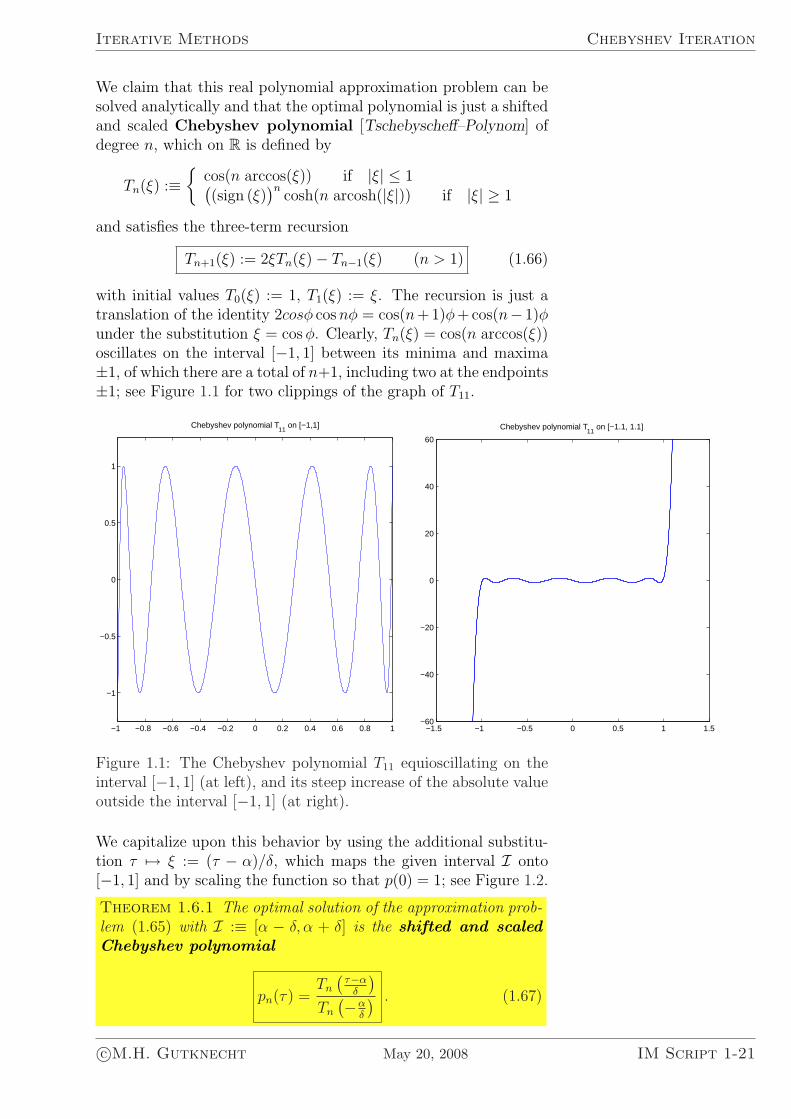
with initial values T0(ξ) := 1, T1(ξ) := ξ. The recursion is just atranslation of the identity 2cosφ cos nφ = cos(n+1)φ+cos(n− 1)φunder the substitution ξ = cos φ. Clearly, Tn(ξ) = cos(n arccos(ξ))oscillates on the interval [−1, 1] between its minima and maxima±1, of which there are a total of n+1, including two at the endpoints±1; see Figure 1.1 for two clippings of the graph of T11.
−1 −0.8 −0.6 −0.4 −0.2 0 0.2 0.4 0.6 0.8 1
−1
−0.5
0
0.5
1
Chebyshev polynomial T11
on [−1,1]
−1.5 −1 −0.5 0 0.5 1 1.5−60
−40
−20
0
20
40
60
Chebyshev polynomial T11
on [−1.1, 1.1]
Figure 1.1: The Chebyshev polynomial T11 equioscillating on theinterval [−1, 1] (at left), and its steep increase of the absolute valueoutside the interval [−1, 1] (at right).
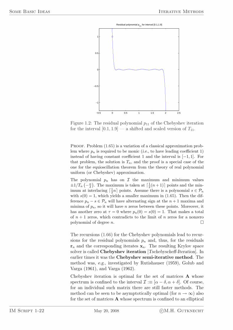
We capitalize upon this behavior by using the additional substitu-tion τ 7→ ξ := (τ − α)/δ, which maps the given interval I onto[−1, 1] and by scaling the function so that p(0) = 1; see Figure 1.2.
Theorem 1.6.1 The optimal solution of the approximation prob-lem (1.65) with I :≡ [α − δ, α + δ] is the shifted and scaledChebyshev polynomial
pn(τ) =Tn
(τ−α
δ
)
Tn
(−αδ
) . (1.67)
c©M.H. Gutknecht May 20, 2008 IM Script 1-21
Some Basic Ideas Iterative Methods
−0.5 0 0.5 1 1.5 2 2.5
−1
−0.5
0
0.5
1
Residual polynomial p11
for interval [0.1,1.9]
Figure 1.2: The residual polynomial p11 of the Chebyshev iterationfor the interval [0.1, 1.9] — a shifted and scaled version of T11.
Proof. Problem (1.65) is a variation of a classical approximation prob-lem where pn is required to be monic (i.e., to have leading coefficient 1)instead of having constant coefficient 1 and the interval is [−1, 1]. Forthat problem, the solution is Tn, and the proof is a special case of theone for the equioscillation theorem from the theory of real polynomialuniform (or Chebyshev) approximation.
The polynomial pn has on I the maximum and minimum values±1/Tn
(−αδ
). The maximum is taken at d1
2(n + 1)e points and the min-imum at interlacing d1
2ne points. Assume there is a polynomial s ∈ Pn
with s(0) = 1, which yields a smaller maximum in (1.65). Then the dif-ference pn − s ∈ Pn will have alternating sign at the n + 1 maxima andminima of pn, so it will have n zeros between these points. Moreover, ithas another zero at τ = 0 where pn(0) = s(0) = 1. That makes a totalof n + 1 zeros, which contradicts to the limit of n zeros for a nonzeropolynomial of degree n. ¤
The recursions (1.66) for the Chebyshev polynomials lead to recur-sions for the residual polynomials pn and, thus, for the residualsrn and the corresponding iterates xn. The resulting Krylov spacesolver is called Chebyshev iteration [Tschebyscheff-Iteration]. Inearlier times it was the Chebyshev semi-iterative method. Themethod was, e.g., investigated by Rutishauser (1959), Golub andVarga (1961), and Varga (1962).
Chebyshev iteration is optimal for the set of matrices A whosespectrum is confined to the interval I :≡ [α− δ, α + δ]. Of course,for an individual such matrix there are still faster methods. Themethod can be seen to be asymptotically optimal (for n →∞) alsofor the set of matrices A whose spectrum is confined to an elliptical
IM Script 1-22 May 20, 2008 c©M.H. Gutknecht
Iterative Methods Chebyshev Iteration
domain E with foci α−δ and α+δ that does not contain the origin.But, in general, it is not optimal in this case, see Fischer and Freund(1990) and Fischer and Freund (1991): exceptions exists even withα, δ ∈ R. Moreover, in the case where A is not real symmetric orHermitian, the factor κ(U) in (1.60) will normally not be 1.
Although our derivation is limited to the case of eigenvalues in areal interval I, we formulate the method here so that the case ofcomplex eigenvalues is included.
Algorithm 1.1 (Chebyshev Iteration) .For solving Ax = b choose x0 ∈ EN and let r0 := b −Ax0. Setr−1 := x−1 := o.Choose the parameters α and δ so that the spectrum of A lies onthe interval I :≡ [α − δ, α + δ] or on an elliptical domain E withfoci α ± δ, but so that 0 6∈ I or 0 6∈ E , respectively. Then letη :≡ −α/δ,
β−1 := 0 , β0 :=δ
2
1
η= − δ2
2α, γ0 := −α , (1.68a)
and compute, for n = 0, 1, . . . until convergence,
βn−1 :≡ δ
2
Tn−1(η)
Tn(η):=
(δ
2
)21
γn−1
if n ≥ 2, (1.68b)
γn :≡ δ
2
Tn+1(η)
Tn(η):= −(α + βn−1) if n ≥ 1, (1.68c)
xn+1 := −(rn + xnα + xn−1βn−1
)/γn , (1.68d)
rn+1 :=(Arn − rnα− rn−1βn−1
)/γn . (1.68e)
Note that in the case of real foci, η :≡ −α/δ < −1, so that in(1.68b) and (1.68c) the formula Tn(η) = (−1)n cosh(n arcosh(−η))should be used.
For the Chebyshev iteration we can specify a bound for the residualnorm reduction and thus estimate the speed of convergence. Thisrequires a little bit more classical analysis; additionally, complexanalysis is also helpful for understanding the background of themethod.
Let us again assume that A is Hpd and that its spectrum is knownto be in I = [α− δ, α + δ], where α > δ > 0. Moreover, let us set
κI :≡ α + δ
α− δ. (1.69)
Note that κI is a bound for the spectral condition number κ(A),and that κI = κ(A) if I is chosen smallest possible, that is so thatα± δ are the smallest and the largest eigenvalues of A. Recall thatthe two bounds in (1.64) hold. The one in the middle,
‖rn‖/‖r0‖ ≤ maxi=1,...,N
|pn(λi)| , (1.70)
is sharp in the sense that for any n we can specify an x0 so that
c©M.H. Gutknecht May 20, 2008 IM Script 1-23
Some Basic Ideas Iterative Methods
equality holds. In fact, if m is the index for which the maximum istaken in (1.70), and if um is the eigenvector corresponding to λm,then we just need to choose x0 := x?−um. Then r0 = A(x?−x0) =umλm and rn = umλmpn(λm) = r0pn(λm).
Since (τ − α)/δ ∈ [−1, 1] if τ ∈ I we conclude further that
maxi=1,...,N
|pn(λi)| = |pn(λm)| ≤ 1∣∣Tn
(−αδ
)∣∣ =1
|Tn(η)| . (1.71)
Here, since η < −1, we have |Tn(η)|−1 < 1, which means that‖rn‖ < ‖r0‖ if n > 0. The bound in (1.71) is sharp in the sensethat there are matrices with spectrum contained in I for whichequality holds.
As is easy to verify, ϑ :≡ exp(arcosh(−η)
)> 1 satisfies
1
2
(ϑ +
1
ϑ
)= −η . (1.72)
In terms of ϑ the value Tn(η) can be written as
Tn(η) =(−1)n
2
(ϑn +
1
ϑn
). (1.73)
Relation (1.72), which, up to the minus sign, describes theJoukowski transformation (Henrici, 1974), means that ϑ2 +2ηϑ + 1 = 0 and yields
ϑ = −η ±√
η2 − 1. (1.74)
In terms of κI we have from (1.69)
η = −κI + 1
κI − 1, (1.75)
and, after some manipulation, we find the two reciprocal solutions
ϑ =
√κI + 1√κI − 1
or ϑ =
√κI − 1√κI + 1
, (1.76)
which both yield
|Tn(η)| = 1
2
[(√κI + 1√κI − 1
)n
+
(√κI − 1√κI + 1
)n]. (1.77)
Actually, only the first solution, the one with ϑ > 1 is consistentwith our definition of ϑ based on the principal branch of arcosh. Insummary, (1.70), (1.71), and (1.77) yield the following estimate.
Theorem 1.6.2 The residual norm reduction of the Chebysheviteration, when applied to an Hpd system whose condition numberis bounded by κI, is bounded according to
‖rn‖‖r0‖ ≤ 2
[(√κI + 1√κI − 1
)n
+
(√κI − 1√κI + 1
)n]−1
≤ 2
(√κI − 1√κI + 1
)n
.
(1.78)The first bound is sharp in the sense that there are matrices Awith spectrum in I and suitable initial vectors x0 such that thebound is attained.
IM Script 1-24 May 20, 2008 c©M.H. Gutknecht
Iterative Methods Chebyshev Iteration
The theorem means that, in general, the residuals in the Chebysheviteration converge linearly. The asymptotic (root-)convergencefactor is bounded according to
(‖rn‖‖r0‖
)1/n
≤√
κI − 1√κI + 1
=1
ϑ= e−arcosh(−η) = |η| −
√η2 − 1 .
(1.79)
Using some of the formulas given above, it is easy to show thatthe coefficients βn and γn of the Chebyshev iteration converge asn →∞, that is βn → β and γn → γ. In fact, from (1.73) we have
Tn−1(η)
Tn(η)= − ϑn−1 + ϑ−(n−1)
ϑn + ϑ−n→ − 1
ϑas n →∞ .
Therefore, by (1.68b) and (1.68c), we have
βn−1 → β :≡ − δ
2ϑ= − δ
2
(|η| −
√η2 − 1
), (1.80)
γn → γ :≡ − δϑ
2= − δ
2
(|η|+
√η2 − 1
), (1.81)
and thus
β + γ = −δ
2
(ϑ + ϑ−1
)= δη = −α , (1.82)
as required by the limit of (1.68c).
Redefining in the recursions (1.68d) and (1.68e) γ0 := −α andβn−1 := β, γn := γ if n > 0, we obtain another Krylov spacesolver, which is also asymptotically optimal for the same intervaland the same set of confocal ellipses. It is called second-orderRichardson iteration. In contrast to the Chebyshev iteration ituses a stationary three-term recursion for rn, that is, the coefficientsdo not depend on n. Actually, the recursion involves again fourterms, but the underlying recursion for the residual polynomialshas only three terms if we write τpn(τ)− αpn(τ) as (τ − α)pn(τ).
Like for SOR, the main disadvantage of these two methods is thatsome knowledge of the spectrum of A is required, in particular alower bound for the distance of the smallest eigenvalue from theorigin.
c©M.H. Gutknecht May 20, 2008 IM Script 1-25
Some Basic Ideas Iterative Methods
1.7 Preconditioning
When applied to large real-world problems Krylov space solversoften converge very slowly — if at all. In practice, Krylov spacesolvers are therefore nearly always applied with preconditioning[Vorkonditionierung, Prakonditionierung ]. The basic idea behind itis to replace the given linear system Ax = b by an equivalent onewhose matrix is more suitable for a treatment by the chosen Krylovspace method. In particular, it is normally expected to have muchbetter condition. Ideal are matrices whose eigenvalues are clusteredaround one point except for a few outliers, and such that the clusteris well separated from the origin. Other properties, like the degreeof nonnormality, also play a role, since highly nonnormal matricesoften cause a delay of the convergence. Minor perturbations of suchmatrices can cause the spectrum to change much. Note that again,this new matrix needs not be available explicitly.
There are several ways of preconditioning. In the simplest case,called left preconditioning [linke Vorkonditionierung ], the sys-tem is just multiplied from the left by some matrix C that is insome sense an approximation of the inverse of A:
CA︸︷︷︸A
x = Cb︸︷︷︸b
. (1.83)
C is then called a left preconditioner [linker Vorkonditionierer]or, more appropriately, an approximate inverse [approximativeInverse] applied on the left-hand side. Of course, C should be sparseor specially structured, so that the matrix-vector product Cy canbe calculated quickly for any y.
Often, given is not C but its inverse M :≡ C−1, which is also calledleft preconditioner. In this case, we need to be able to solveMz = y quickly for any y.
An alterative is to substitute x by x :≡ C−1x, so that Ax = b isreplaced by
AC︸︷︷︸A
C−1x︸ ︷︷ ︸x
= b . (1.84)
This is right preconditioning [rechte Vorkonditionierung ]. Here,logically, C is called a right preconditioner [rechter Vorkondi-tionierer] or, an approximate inverse applied on the right-hand side.Again, we may not have C available but its inverse M. Note thatin the situation of (1.84) we do not need C−1 because we will firstobtain x and so have to compute x = Cx.
Sometimes it is most appropriate to combine these approaches byso-called split preconditioning [gesplittete Vorkonditionierung ].
In general, the effect of preconditioning on the formulation andconvergence of a Krylov space solver can be understood as the re-
IM Script 1-26 May 20, 2008 c©M.H. Gutknecht
Iterative Methods Preconditioning
placement of the system Ax = b by
CLACR︸ ︷︷ ︸A
C−1R x︸ ︷︷ ︸x
= CLb︸︷︷︸b
, (1.85)
where we allow either CL or CR to be the identity, or by
M−1L AM−1
R︸ ︷︷ ︸A
MRx︸ ︷︷ ︸x
= M−1L b︸ ︷︷ ︸b
, (1.86)
where now at most either ML or MR is the identity. The productC :≡ CL CR or the product M :≡ MR ML, respectively, is calledsplit preconditioner [gesplitteter Vorkonditionierer].
Split preconditioning is particularly useful if A is real symmetric (orHermitian) and we choose as the right preconditioner the transpose(or, in the complex case, the Hermitian transpose) of the left one,
so that A is still symmetric. In particular, if MR and CL are lowertriangular matrices L and K, respectively, we have
M = LL? , C = KK? , (1.87)
and these can be viewed as the Cholesky decompositions[Cholesky-Zerlegungen] of M and C, respectively.
Left preconditioning effects the residuals: it involves the precon-ditioned residual vectors
rn :≡ CL rn = M−1L rn = M−1
L (bn −Axn) . (1.88)
On the other hand, right preconditioning effects the error vectors:it involves the preconditioned error vectors
xn − x? :≡ MR (xn − x?) = MR dn = C−1R (xn − x?) . (1.89)
Of course, the difficult part in preconditioning is to find the pre-conditioner, be it CL, CR, ML, MR, L, or K. Yet another questionis how to efficiently combine the Krylov space solver with the pre-conditioner. Of course, one could just replace A, b, and x by A,b, and x, but there are sometimes more efficient ways to build apreconditioner into a Krylov space solver. We will treat such casesin Section 2.7, where, in various ways, preconditioning is built intoconjugate gradient algorithms.
c©M.H. Gutknecht May 20, 2008 IM Script 1-27
Some Basic Ideas Iterative Methods
1.8 Some Basic Preconditioning Techniques
1.8.1 Preconditioning based on classical matrix splittings
Recall from Section 1.4 that a matrix splitting A = M −N withappropriately chosen N may be used to speed up the linear fixedpoint iteration
xn+1 := Bxn + b with B :≡ I−A (1.90)
by replacing it by
xn+1 := Bxn + b (1.91)
with
B :≡ M−1N = M−1(M−A) , b :≡ M−1b . (1.92)
While (1.90) is the straightforward fixed point iteration for thelinear system Ax = b, the modified iteration (1.91)–(1.92) is thefixed point iteration for the left-preconditioned system M−1Ax =M−1b.
So the methods based on matrix splittings that we discussed inSection 1.4 can all be understood as linear fixed point iterationsfor preconditioned systems. There the aim of the preconditioningwas to make the spectral radius ρ(B) as small as possible, sincethis spectral radius equals the asymptotic rate of convergence. Inany case it has to be smaller than 1, since this is a necessary andsufficient condition for convergence for all x0. This condition alsoguarantees that A :≡ M−1A = I− B is nonsingular.
The same preconditioners M can also be used with other Krylovspace solvers. For example, we could use the matrix M from ablock Jacobi splitting or the one from an SSOR splitting as a leftpreconditioner in the Chebyshev method or in many of the Krylovspace solvers we will discuss later. This simple approach to precon-ditioning is quite popular. Note that here the preconditioning hasthe effect that all eigenvalues of A lie in a circle of radius ρ(B) < 1around the point 1. We do not iterate with, say block Jacobi orSSOR, but we only use the underlying splitting to obtain a betterconditioned matrix A. In some sense, we combine each step of theKrylov space solver with one step of the iteration based on splitting.
The SOR splitting is not appropriate for preconditioning. In thiscase, as we mentioned, if A has Property A and is consistentlyordered, and if D−1A has real eigenvalues, then the eigenvalues ofB lie for the optimal ω on the circle with radius ρ(B) < 1 and center
0, those of A lie on a circle with the same radius but center 1. Thiskind of spectrum is not very suitable for Krylov space solvers unlessρ(B) is really small.
IM Script 1-28 May 20, 2008 c©M.H. Gutknecht
Iterative Methods Some Basic Preconditioning Techniques
1.8.2 Incomplete LU and Cholesky factorizations
If we knew a Gaussian LU factorization of A, say A = PTLU witha permutation matrix P, a lower triangular matrix L, and an uppertriangular matrix U, we could choose
M :≡ PTLU (1.93)
as a left preconditioner, which means that A = M−1A = I would beoptimally preconditioned. Application of this preconditioner wouldrequire to forward substitute with U, back substitute with L, andto permute components according to P. But application of M−1 tor0 would yield in one step
x? = x0 − d0 = x0 + M−1r0 . (1.94)
Of course, when we choose x0 := o, so that r0 = b, then this isessentially just the application of Gauss elimination.
As we mentioned in Section 1.2 the problem with the LU factoriza-tion is that for most large sparse matrices (except for banded oneswith a very dense band) this approach is inefficient because theLU factors are much denser than A and thus their computation iscostly and their memory requirement is large. The set of additionalnonzero elements in L and U in positions of zero elements in A iscalled fill-in.
An often very effective alternative is to compute an approximateLU factorization that is as sparse as A or at least nearly assparse: we choose sparse matrices L and U and a permutationmatrix P so that the difference LU − PA is small. The prod-uct M :≡ PTLU ≈ A is then called an incomplete LU (ILU)factorization [unvollstandige LU-Zerlegung ]. For the case of spdand Hpd matrices there are analogous products M :≡ LLT ≈ Acalled incomplete Cholesky (IC) factorization [unvollstandigeCholesky-Zerlegung ].
There are many variants of ILU and IC factorizations. Often,no pivoting is used even in the unsymmetric ILU decomposition;that is, P = I. In the simplest variant we compute an LU or aCholesky factorization, but where A has a zero element we replaceany nonzero element of L or U by a zero. That is, zero fill-in isenforced.
The next step of sophistication is to prescribe some pattern[Muster] P of forced zeros:
P ⊆ {(i, j)
∣∣ i 6= j, ai,j = 0, 1 ≤ i ≤ N, 1 ≤ j ≤ N}
. (1.95)
One version of the corresponding ILU factorization algorithm with-out pivoting looks as follows:
c©M.H. Gutknecht May 20, 2008 IM Script 1-29

Some Basic Ideas Iterative Methods
Algorithm 1.2 (ILU factorization with fixed pattern P )
for k = 1, . . . , n− 1 dofor i = k + 1, . . . , n do
if (i, k) 6∈ P ,aik := aik/akk ;for j = k + 1, . . . , n do
if (i, j) 6∈ P ,aij := aij − aik ∗ akj ;
endifendfor
endifendfor
endfor
Of course, there is no guarantee that this decomposition exists, evenwhen A is nonsingular, since we do not include pivoting here. Butworse, the ILU decomposition may not exist even when the full LUdecomposition of A exists. For example, even when A is spd, theILU decomposition or the corresponding IC decomposition need notexist. But there are classes of matrices for which it can be shownthat the ILU decomposition exists, at least in exact arithmetic.
It is easy to show that after the ILU decomposition — if it can becompleted — holds
A = LU−R , (1.96)
wherelij = 0 if i < j or (i, j) ∈ P ,uij = 0 if i < j or (i, j) ∈ P ,rij = 0 if (i, j) 6∈ P .
(1.97)
If one wants to avoid the assumption (i, j) ∈ P =⇒ ai,j = 0 inthe definition of P , then one needs the following assignment beforeexecuting the algorithm
∀(i, j) ∈ P with aij 6= 0 : rij := −aij , aij := 0 . (1.98)
But this is hardly ever required in practice.
In other versions of ILU algorithms the pattern P is not fixed inadvance, but depends on the sizes of the matrix elements that areconstructed: any constructed small element of L or U is deletedon the spot by comparison with a threshold (drop tolerance) T .This version is called ILUT. A detailed treatment of various ILUalgorithms is given in Saad (1996).
Matlab provides for example:
[L,U,P] = luinc(A,’0’): ILU with pivoting, no fill-in[L,U,P] = luinc(A,droptol): ILUT with pivoting[L,U,P] = cholinc(A,’0’): IC with no fill-in[L,U,P] = cholinc(A,droptol): IC with drop tolerance
IM Script 1-30 May 20, 2008 c©M.H. Gutknecht
Iterative Methods Some Basic Preconditioning Techniques
1.8.3 Polynomial preconditioning
Given A and c, a Krylov space solver applied to Aw = c deliversapproximations w` of w? :≡ A−1c, and according to (1.53) we have,when choosing w0 := o,
w` = q`−1(A)c ∈ K`(A, c) . (1.99)
In some Krylov space solvers, the polynomial q`−1 ∈ P`−1 dependson the right-hand side c, but in others, like Jacobi or Chebysheviteration, it does not. Let us assume the latter case. Then q`−1(A)can be viewed as an operator that maps any c into an approximationof A−1c. In particular, if c := Aw is considered as an image pointof A (and if A is nonsingular, it always can be considered so), thenq`−1(A)A can be viewed as an approximation of the identity. So,C := q`−1(A) is an approximate inverse of A. It is often calledpolynomial preconditioner [polynomialer Prakonditionierer].
In summary: given any Krylov space solver whose recurrence coeffi-cients only depend on A but not on c, and given any fixed iterationnumber `, if q`−1 ∈ P`−1 is the polynomial representing the `th iter-ate w` when solving Aw = c, then C := q`−1(A) is an approximateinverse of A.
To implement this preconditioner for computing, say, CAz, we firstcompute c := Az and then perform ` steps of the Krylov spacesolver applied to Aw = c; so that w` = CAz.
As early as 1959, it was suggested by Rutishauser (1959) to useChebyshev iteration in this way as a preconditioner (although thenotion of “preconditioning” did not yet exist at that time).
1.8.4 Inner-outer iteration
A natural generalization of polynomial preconditioning is to allowany Krylov space solver, even one where q`−1 depends on c, and alsoto allow ` to vary from one application of C to the next; so we shouldwrite Cn when applying the inner iteration [innere Iteration] thenth time, that is, in the nth step of the outer iteration [aussereIteration]. Instead of choosing ` in advance, we may then terminateeach inner iteration when the inner residual
cn −Awn,`n = cn −A qn,`n−1(A)︸ ︷︷ ︸≡: Cn
cn = (I−Aqn,`n−1(A))︸ ︷︷ ︸≡: pn,`n(A)
cn
is considered small enough. It need not be very small. The com-bination of such a flexible preconditioning [flexible Vorkondi-tionierung ] with a Krylov space solver as outer iteration is calledinner-outer iteration and has become very fashionable.
c©M.H. Gutknecht May 20, 2008 IM Script 1-31

Some Basic Ideas Iterative Methods
IM Script 1-32 May 20, 2008 c©M.H. Gutknecht
Iterative Methods Energy Norm Minimization
Chapter 2
The Conjugate Gradient Method
2.1 Energy Norm Minimization
In many areas of science and technology stable states are charac-terized by minimum energy. Discretization then leads in the firstapproximation to the minimization of a quadratic function in sev-eral variables,
Ψ(x) :≡ 12xTAx− bTx + γ (2.1)
with an spd matrix A. (We assume real data in Sections 2.1–2.6.)Such a function Ψ is well known to be convex since its secondderivative is the matrix A. So it has a unique minimum, which canbe found by setting the first derivative, the gradient, equal to o.The gradient can be seen to be
∇Ψ(x) = Ax− b = −r , (2.2)
where r is the residual corresponding to x. Hence,
x minimizer of Ψ ⇐⇒ ∇Ψ(x) = o ⇐⇒ Ax = b .
(2.3)As before, we let x? be the minimizer, i.e., the solution of Ax = b,and d :≡ x−x? be the error of x. If we define the A-norm as usualby
‖y‖A :≡√
yTAy , (2.4)
it is easily seen that
‖d‖2A = ‖x− x?‖2
A = ‖Ax− b‖2A−1 = ‖r‖2
A−1 = 2 Ψ(x) (2.5)
if in (2.1)γ :≡ 1
2bTA−1b . (2.6)
Of course, the value of the constant γ has no influence on the solu-tion, so we can assume from now on that we have made this choice;thus, in other words, we are minimizing the A-norm of the error,which is often referred to as the energy norm [Energienorm].
In summary: If A is spd, to minimize the quadratic function Ψmeans to minimize the energy norm of the error vector of the linearsystem Ax = b.
Since A is spd, the level curves Ψ(x) = const are ellipses if N = 2and ellipsoids if N = 3.
c©M.H. Gutknecht May 20, 2008 IM Script 2-1
CG and Symmetric Lanczos Iterative Methods
2.2 Steepest Descent
The interpretation of the solution of a linear system as the min-imizer of convex quadratic function Ψ suggests to find this mini-mizer by moving down the surface representing Ψ in the directionof steepest descent given by minus the gradient.
However, to follow approximately the so defined curve would requireto make many small steps and to evaluate the gradient at everystep. We prefer to follow a piecewise straight line with rather longpieces, that is, to make a long step whenever the gradient and thusthe direction of steepest descent has been computed. So, in the nthstep, we proceed from (xn, Ψ(xn)) on a straight line in the oppositedirection of the gradient ∇Ψ(x), that is, in the direction of rn. Anatural choice is to go to the point with the minimum value of Ψon that line. In general, finding the minimum value of a functionalon a line is called line search, but here, since Ψ is quadratic, thelength of the step is easy to compute. On the line
ω 7→ xn + rnω (2.7)
the minimum
xn+1 := xn + rnωn (2.8)
of ‖xn+1 − x?‖2A = ‖rn+1‖2
A−1 is readily found: xn+1 = xn + rnωn
implies that rn+1 = rn −Arnωn, so that
‖rn+1‖2A−1 = ‖rn −Arnωn‖2
A−1
= ‖rn‖2A−1 − 2 〈rn,Arn〉A−1 ωn + ‖Arn‖2
A−1 ω2n
= ‖rn‖2A−1 − 2 〈rn, rn〉 ωn + 〈rn,Arn〉 ω2
n .
As a function of ωn, this expression has a vanishing derivative (andis thus minimal) when
ωn :≡ 〈rn, rn〉〈rn,Arn〉 . (2.9)
This is the method of steepest descent [Methode des steilstenAbstiegs]. Comparing its formulas (2.8) and (2.9) with (1.21) we seethat it differs from the Jacobi iteration only in the (locally optimal)choice of the step length.
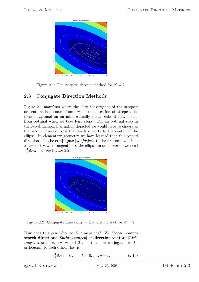
However, this method may converge very slowly even if N is only2. This is easily seen if we assume that N = 2 and that the two(positive) eigenvalues of A differ very much in size. Then the levelcurves of Ψ are concentric ellipses with a large axis ratio of λ1/λ2,and the search directions are orthogonal to these ellipses. Obvi-ously, there are situations, where it takes many steps to come closeto the center of the ellipses; see Figure 2.1. It is also clear that, ingeneral, this method does not converge in at most N steps.
IM Script 2-2 May 20, 2008 c©M.H. Gutknecht
Iterative Methods Conjugate Direction Methods
−3 −2 −1 0 1 2 3 4 5 6 7 8
−7
−6
−5
−4
−3
−2
−1
0
1
2
3
4Steepest descent method
x0
x1
x2
x3
x4
x*
Figure 2.1: The steepest descent method for N = 2.
2.3 Conjugate Direction Methods
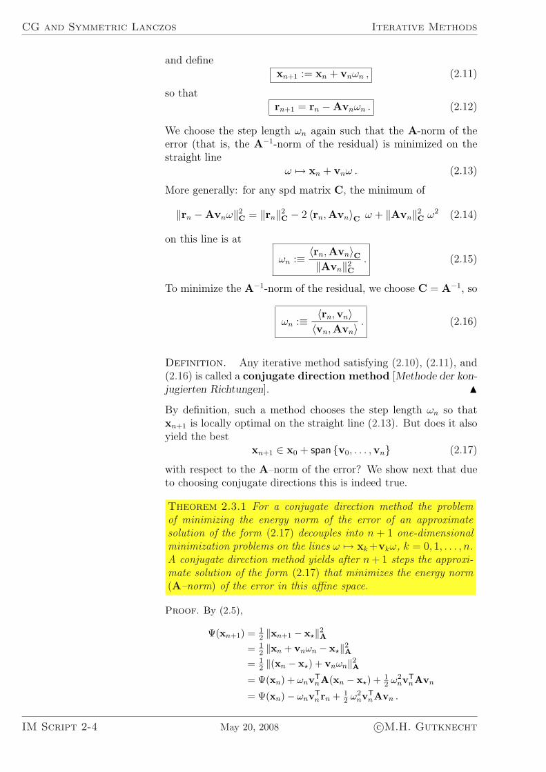
Figure 2.1 manifests where the slow convergence of the steepestdescent method comes from: while the direction of steepest de-scent is optimal on an infinitesimally small scale, it may be farfrom optimal when we take long steps. For an optimal step inthe two-dimensional situation depicted we would have to choose asthe second direction one that leads directly to the center of theellipse. In elementary geometry we have learned that this seconddirection must be conjugate [konjugiert] to the first one, which atx1 := x0 +v0ω0 is tangential to the ellipse; in other words, we needvT
1 Av0 = 0, see Figure 2.2.
−3 −2 −1 0 1 2 3 4 5 6 7 8−8
−6
−4
−2
0
2
4Conjugate gradient method
x0
x1
x*
Figure 2.2: Conjugate directions — the CG method for N = 2.
How does this generalize to N dimensions? We choose nonzerosearch directions [Suchrichtungen] or direction vectors [Rich-tungsvektoren] vn (n = 0, 1, 2, . . . ) that are conjugate or A–orthogonal to each other, that is
vTnAvk = 0 , k = 0, . . . , n− 1, (2.10)
c©M.H. Gutknecht May 20, 2008 IM Script 2-3
CG and Symmetric Lanczos Iterative Methods
and definexn+1 := xn + vnωn , (2.11)
so thatrn+1 = rn −Avnωn . (2.12)
We choose the step length ωn again such that the A-norm of theerror (that is, the A−1-norm of the residual) is minimized on thestraight line
ω 7→ xn + vnω . (2.13)
More generally: for any spd matrix C, the minimum of
‖rn −Avnω‖2C = ‖rn‖2
C − 2 〈rn,Avn〉C ω + ‖Avn‖2C ω2 (2.14)
on this line is at
ωn :≡ 〈rn,Avn〉C‖Avn‖2
C
. (2.15)
To minimize the A−1-norm of the residual, we choose C = A−1, so
ωn :≡ 〈rn,vn〉〈vn,Avn〉 . (2.16)
Definition. Any iterative method satisfying (2.10), (2.11), and(2.16) is called a conjugate direction method [Methode der kon-jugierten Richtungen]. N
By definition, such a method chooses the step length ωn so thatxn+1 is locally optimal on the straight line (2.13). But does it alsoyield the best
xn+1 ∈ x0 + span {v0, . . . ,vn} (2.17)
with respect to the A–norm of the error? We show next that dueto choosing conjugate directions this is indeed true.
Theorem 2.3.1 For a conjugate direction method the problemof minimizing the energy norm of the error of an approximatesolution of the form (2.17) decouples into n + 1 one-dimensionalminimization problems on the lines ω 7→ xk +vkω, k = 0, 1, . . . , n.A conjugate direction method yields after n + 1 steps the approxi-mate solution of the form (2.17) that minimizes the energy norm(A–norm) of the error in this affine space.
Proof. By (2.5),
Ψ(xn+1) = 12 ‖xn+1 − x?‖2
A
= 12 ‖xn + vnωn − x?‖2
A
= 12 ‖(xn − x?) + vnωn‖2
A
= Ψ(xn) + ωnvTnA(xn − x?) + 1
2 ω2nv
TnAvn
= Ψ(xn)− ωnvTnrn + 1
2 ω2nv
TnAvn .
IM Script 2-4 May 20, 2008 c©M.H. Gutknecht
Iterative Methods The Conjugate Gradient (CG) method
As a consequence of (2.10) we get
vTnrn = vT
n (r0 + A(x0 − xn))
= vTnr0 − vT
nA(v0ω0 + · · ·+ vn−1ωn−1)
= vTnr0 .
Therefore,
Ψ(xn+1) = Ψ(xn)− ωnvTnr0 + 1
2 ω2nv
TnAvn . (2.18)
Here, the last two terms on the right-hand side are independent of v0,. . . , vn−1 and ω0, . . . , ωn−1. So from (2.18) we conclude that the prob-lem of finding the global minimum with respect to the search direc-tions v0, . . . ,vn decouples into the one of minimizing with respect tov0, . . . ,vn−1 (which by induction we may assume to yield xn) and theone-dimensional minimization (line search) with respect to vn. The op-timal ωn in (2.18) is given by ωn = (vT
nr0)/(vTnAvn), but in view of
(2.10) this yields the same as (2.16). By induction, finding the globalminimum of Ψ(xn) decouples further into n one-dimensional minimumproblems. ¤
Conjugate direction methods in this general sense, as well as thespecial case of the conjugate gradient method treated next havebeen introduced by Hestenes and Stiefel (1952).
2.4 The Conjugate Gradient (CG) method
In general, conjugate direction methods are not Krylov spacesolvers, but if we choose the search directions in a suitable Krylovsubspace, we obtain one. From the relation
xn+1 = x0 +v0ω0 + · · ·+vnωn ∈ x0 + span {v0,v1, . . . ,vn} (2.19)
we see that we need to choose search directions v0, . . . ,vn so that
span {v0, . . . ,vn} = Kn+1(A, r0) , n = 0, 1, 2, . . . . (2.20)
Actually, we need primarily that span {v0, . . . ,vn} ⊆ Kn+1, but theconjugacy condition (2.10) and the requirement vn 6= 0 imply thatequality must hold.
Definition. The conjugate gradient (CG) method [Meth-ode der konjugierten Gradienten] is the conjugate direction methodwith the choice (2.20). N
Theorem 2.3.1 immediately leads to the main result on this method:
Theorem 2.4.1 The CG method yields approximate solutionsxn ∈ x0 + Kn(A, r0) that are optimal in the sense that they min-imize the energy norm (A–norm) of the error vector for xn fromthis affine space, or, equivalently, it minimizes the A−1–norm ofthe residual.
c©M.H. Gutknecht May 20, 2008 IM Script 2-5
CG and Symmetric Lanczos Iterative Methods
By the two conditions (2.10) and (2.20) the search directions vn
have to satisfy, they are uniquely determined up to a scalar factor.But how can we construct them efficiently?
We note that if rn ∈ Kn+1\Kn, we may normalize vn so that
vn − rn ∈ Kn . (2.21)
Before we can proceed we need
Lemma 2.4.2 The CG method produces mutually orthogonalresiduals:
rTnrk = 0 , k = 0, . . . , n− 1 . (2.22)
So, if r0, . . . , rn−1 6= o,
span {r0, . . . , rn−1} = Kn(A, r0) ⊥ rn . (2.23)
Proof. Let us insert the optimal ωn of (2.16) into the update formula(2.12) for rn:
rn+1 = rn −Avnωn
= rn −Avn〈rn,vn〉〈vn,Avn〉 . (2.24)
By induction, assuming that o 6= rk ⊥ Kk for k ≤ n, which implies that(2.23) holds, we see using (2.21) and (2.10), respectively, that
〈rn, rn〉 = 〈rn,vn〉 , 〈rn,Avn〉 = 〈vn,Avn〉 . (2.25)
Multiplying (2.24) from the left by rTn we conclude that rn+1 ⊥ rn. And
multiplying it by rTk with k < n shows likewise that rn+1 ⊥ rk. So,
(2.22) and (2.23) hold with n replaced by n + 1. ¤
Note that in the formula (2.16) for ωn we can replace 〈rn,vn〉 by〈rn, rn〉; see (2.25). So,
ωn =〈rn, rn〉〈vn,Avn〉 =
δn
δ′n, (2.26)
where δn :≡ 〈rn, rn〉, δ′n :≡ 〈vn,Avn〉.
In view of the above we can choose
vn+1 := rn+1 − linear combination of v0,v1, . . . ,vn .
But we may try the simpler ansatz
vn+1 := rn+1 − vnψn . (2.27)
Since Avk ∈ Kn+1 for k < n, we find from Lemma 2.4.2 that(Avk)
Trn+1 = 0 for k < n. Therefore, by multiplying (2.27) fromthe left by (Avk)
T with k < n we see that 〈vn+1,Avk〉 = 0 (k < n)as required. Moreover, we also get 〈vn+1,Avn〉 = 0 if we choose
IM Script 2-6 May 20, 2008 c©M.H. Gutknecht
Iterative Methods The Conjugate Gradient (CG) method
ψn = 〈rn+1,Avn〉 / 〈vn,Avn〉. Substituting in numerator and de-nominator Avn = (rn − rn+1)
1ωn
(from the update formula (2.21)for rn) and making use of 〈vn, rn〉 = 〈rn, rn〉 we finally obtain
ψn :≡ 〈rn+1,Avn〉〈vn,Avn〉 = − 〈rn+1, rn+1〉
〈rn, rn〉 = − δn+1
δn
. (2.28)
Putting things together we now get a detailed algorithm for the CGmethod. We will see that there exist other algorithms using differ-ent recursions, but here we get the (standard) Hestenes-Stiefelalgorithm, which is also called coupled two-term version orOMin version of the method. The terminology “coupled two-term” refers to the fact that for both the residuals and the searchdirections two-term recursions, namely (2.12) and (2.27), are usedfor updating. The similar recursion for the iterates xn follows fromthe one for the residuals. Again, these recursions actually containthree terms, but only two belong to the same sequence. The name“OMin” refers to orthogonality and minimality and will be put ina broader context later.
Algorithm 2.1 (OMin form of the CG method) .For solving Ax = b choose an initial approximation x0, and letv0 := r0 := b −Ax0 and δ0 := ‖r0‖2. Then, for n = 0, 1, 2, . . . ,compute
δ′n := ‖vn‖2A , (2.29a)
ωn := δn/δ′n , (2.29b)
xn+1 := xn + vnωn , (2.29c)
rn+1 := rn −Avnωn , (2.29d)
δn+1 := ‖rn+1‖2, (2.29e)
ψn := −δn+1/δn , (2.29f)
vn+1 := rn+1 − vnψn . (2.29g)
If ‖rn+1‖ ≤ tol, the algorithm terminates and xn+1 is a suffi-ciently accurate approximation of the solution.
In Matlab: x = pcg(A,b) , but there are many options:
[X,FLAG,RELRES,ITER,RESVEC] = PCG(A,B,TOL,MAXIT,M1,M2,X0)
These options include: multiple right-hand sides, tolerance, maxi-mum number of iterations, preconditioning, stopping flag, residualnorm, iteration number, residual history.
Since the CG method produces optimal approximations from theaffine spaces x0 + Kn it is clear that it finds the solution in theminimum number of steps, and from Corollary 1.5.5 we know thatν(r0,A) steps are needed:
c©M.H. Gutknecht May 20, 2008 IM Script 2-7
CG and Symmetric Lanczos Iterative Methods
Theorem 2.4.3 The conjugate gradient method yields (in exactarithmetic) the solution of Ax = b in the minimum numberν(r0,A) of steps.
However, it is important to point out that this is a theoretical result,which does not hold in practice due to rounding errors. These oftenhave a very strong effect on the method. Nevertheless, in most casesthe method still converges, and in fact delivers very small residualsin far less than ν(r0,A) steps. We stop when some measure ofthe error is small enough, and ‖rn+1‖ is a simple such measure.However, since the CG method minimizes the energy norm withineach Krylov subspace, it might be more appropriate to check thesize of ‖dn+1‖A = ‖rn+1‖A−1 . Hestenes and Stiefel (1952) alsoshowed how this can be done efficiently.
Next we want to illustrate how the recursions Krylov space solversare based on can be described by matrix equations. We note thatthe recursions (2.29c), (2.29d), and (2.29g) mean that
vn = − (xn − xn+1)1
ωn,
Avn = (rn − rn+1)1
ωn,
rn+1 = vn+1 + vnψn .
If we let
Rm :≡ (r0 r1 · · · rm−1
), (2.30a)
Vm :≡ (v0 v1 · · · vm−1
), (2.30b)
Xm :≡ (x0 x1 · · · xm−1
), (2.30c)
and assume m > n, we can write them as
vn = − (x0 · · · xn−1 xn xn+1 xn+2 . . . xm
)︸ ︷︷ ︸
Xm+1
0...0
ω−1n
−ω−1n
0...0
,
Avn =(
r0 · · · rn−1 rn rn+1 rn+2 . . . rm
)︸ ︷︷ ︸
Rm+1
0...0
ω−1n
−ω−1n
0...0
,
and
IM Script 2-8 May 20, 2008 c©M.H. Gutknecht
Iterative Methods The Conjugate Gradient (CG) method
rn+1 =(
v0 · · · vn−1 vn vn+1 vn+2 . . . vm−1
)︸ ︷︷ ︸
Vm
0...0ψn
10...0
.
Let us further introduce the matrices
Um :≡
1 ψ0
1 ψ1
1. . .. . . ψm−2
1
, (2.31)
L◦m :≡
ω−10
−ω−10 ω−1
1
−ω−11 ω−1
2. . . . . .
−ω−1m−2 ω−1
m−1
−ω−1m−1
, (2.32)
Em :≡
1−1 1
−1 1. . . . . .
−1 1−1
, (2.33)
andDω; m :≡ diag {ω0, ω1, . . . , ωm−1} , (2.34)
so thatL◦m = Em D−1
ω; m . (2.35)
L◦m and Em are “extended” lower bidiagonal matrices of the size(m + 1)×m whose column sums vanish1.
In terms of all these matrices the coupled two-term CG recursions(2.29d) for n = −1, . . . , m− 2 and (2.29g) for n = 0, . . . ,m− 1 canbe summarized as
Rm = VmUm , AVm = Rm+1L◦m (m ≤ ν) , (2.36)
and the additional recursion (2.29c) for the iterates turns into
Vm = −Xm+1L◦m (m ≤ ν) . (2.37)
1By underlining Em we want to indicate that we augment this matrix byan additional row. We suggest reading Em as “E sub m extended”. The samenotation will be used on other occasions.
c©M.H. Gutknecht May 20, 2008 IM Script 2-9
CG and Symmetric Lanczos Iterative Methods
Eliminating the direction vectors contained in Vm yields
ARm = Rm+1T◦m , Rm = −Xm+1T
◦m (m ≤ ν) , (2.38)
whereT◦
m :≡ L◦mUm (2.39)
is an ‘extended’ tridiagonal matrix:
T◦m ≡:
T◦m
γm−1lTm
≡:
α0 β0
γ0 α1 β1
γ1 α2. . .
. . . . . . βm−2
γm−2 αm−1
γm−1
,
(2.40)where lTm is the last row of the unit matrix of size m.
The characteristic property of a matrix Z with column sums 0 is
that eTZ = oT for e :≡ (1 1 . . . 1
)Tof appropriate size. So,
eTL◦m = oT, and therefore also
eTT◦m = eTL◦mUm = oT . (2.41)
Thus, T◦m has column sums zero too: if we let β−1 :≡ 0, then
γn = −αn − βn−1 , n = 0, 1, . . . , m− 1 ≤ ν − 1 . (2.42)
According to (2.38) the CG residuals and iterates satisfy three-termrecursions:
rn+1γn = (Arn − rnαn − rn−1βn−1) , (2.43a)
xn+1γn = −(rn + xnαn + xn−1βn−1) , (2.43b)
but what remains to find are formulas for αn and βn−1. InLemma 2.4.2 we have seen that the residuals are orthogonal toeach other, and, when multiplying (2.43a) from the left by rT
n andrT
n−1 this property gives
αn =rT
nArn
rTnrn
, βn−1 =rT
n−1Arn
rTn−1rn−1
.
Here, since A is symmetric and since the three-term recursion andthe orthogonality property of Lemma 2.4.2 hold,
rTn−1Arn = (Arn−1)
Trn
= (rnγn−1 + rn−1αn−1 + rn−2βn−2)Trn
= rTnrnγn−1 ,
so, we only need to compute two inner products, 〈rn,Arn〉 and〈rn, rn〉 per step since 〈rn−1, rn−1〉 and γn−1 will be known from theprevious step, while γn is computed from (2.42).
IM Script 2-10 May 20, 2008 c©M.H. Gutknecht
Iterative Methods The Conjugate Gradient (CG) method
Summarizing everything we obtain a new algorithm for the CGmethod, which is called three-term version or ORes version ofthe method, the latter because it makes direct use of the orthogo-nality of the residuals.
Algorithm 2.2 (ORes form of the CG method) .For solving Ax = b with an Hpd matrix A, choose an initialapproximation x0, and let r0 := b − Ax0, β−1 := 0, and δ0 :=‖r0‖2. Then, for n = 0, 1, . . . , compute
αn := ‖rn‖2A / δn , (2.44a)
βn−1 := γn−1δn/δn−1 (if n > 0), (2.44b)
γn := −αn − βn−1 , (2.44c)
xn+1 := −(rn + xnαn + xn−1βn−1)/γn , (2.44d)
rn+1 := (Arn − rnαn − rn−1βn−1)/γn , (2.44e)
δn+1 := ‖rn+1‖2 . (2.44f)
If ‖rn+1‖ ≤ tol, the algorithm terminates and xn+1 is a suffi-ciently accurate approximation of the solution.
Of course, Arn, which is needed in (2.44a) and (2.44e), is computedonly once and stored in a temporary vector.
There is yet another version of the CG method. Instead of Vm onecan eliminate Rm in (2.36) to obtain
AVm = Vm+1T′m (m ≤ ν) , (2.45)
where
T′m :≡ Um+1L
◦m (2.46)
is again an ‘extended’ tridiagonal matrix. Here, (2.45) describes a3-term recursion for the direction vectors:
vn+1γ′n = Avn − vnα
′n − vn−1β
′n−1 , (2.47)
where we are free to choose γ′n 6= 0, while α′n and β′n−1 have to bedetermined such that
vTnAvn+1 = 0 , vT
n−1Avn+1 = 0 . (2.48)
It is easy to verify that the search direction are then all conjugateto each other, as required by (2.10). In general, T′
m does not havecolumn sums zero.
To update the residuals and iterates we can use (2.29d) and (2.29c)from the OMin version. Altogether we obtain yet another algo-rithm, which is called ODir version of the CG method, as it makesexplicit usage of the A–orthogonality of the search directions.
c©M.H. Gutknecht May 20, 2008 IM Script 2-11
CG and Symmetric Lanczos Iterative Methods
Algorithm 2.3 (ODir form of the CG method) .For solving Ax = b, choose an initial approximation x0, and letv0 := r0 := b−Ax0, β′−1 := 0.Then, for n = 0, 1, . . . , compute
δ′n := ‖vn‖2A , (2.49a)
ω′n := 〈rn,vn〉 /δ′n , (2.49b)
xn+1 := xn + vnω′n , (2.49c)
rn+1 := rn −Avnω′n , (2.49d)
α′n := ‖Avn‖2/δ′n , (2.49e)
β′n−1 := γ′n−1δ′n/δ′n−1 (if n > 0), (2.49f)
vn+1 := (Avn − vnα′n − vn−1β
′n−1)/γ
′n , (2.49g)
where γ′n 6= 0 can be chosen (e.g., to normalize vn+1).If ‖rn+1‖ ≤ tol, the algorithm terminates and xn+1 is a suffi-ciently accurate approximation of the solution.
Remark. Both in (2.44e) and (2.49g) it is preferable to use themodified Gram-Schmidt algorithm, which also means to modify theformulas (2.44a) for αn and (2.49e) for α′n. But, since there are onlytwo terms to subtract, the difference will be marginal. H
Remark. Each step in the sequence
T◦m à (L◦m, Um ) à T′
m à (L′m, U′m ) (2.50)
is essentially half a step of Rutihauser’s quotient-difference (qd)algorithm (Rutishauser, 1957), except that here the matrices arenot square. H
2.5 The Conjugate Residual (CR) Method
We can replace the aim of minimizing the energy norm consideredin Section 2.1 by the aim of minimizing the 2-norm of the residual.Let us still assume that A is symmetric positive definite (spd), sothat this is the same as minimizing the A2–norm of the error:
‖x− x?‖2A2 = ‖d‖2
A2 = ‖r‖2 = ‖Ax− b‖2 = 2 Ψ(x) (2.51)
if
Ψ(x) :≡ 12xTA2x− bTAx + 1
2bTb . (2.52)
Now we have
∇Ψ(x) = A2x−Ab = −Ar (2.53)
and
x minimizer of Ψ ⇐⇒ ∇Ψ(x) = o ⇐⇒ Ar = o .
(2.54)
IM Script 2-12 May 20, 2008 c©M.H. Gutknecht
Iterative Methods The Conjugate Residual (CR) Method
It should be no surprise that we can develop a variation of theconjugate gradient method adapted to this error norm by replac-ing in the derivations of Sections 2.3 and 2.4 the occurrences ofthe A–inner product by those of the A2–inner product, and theoccurrences of the standard inner product by those of the A–innerproduct. In particular, the search directions are chosen from agrowing sequence of Krylov subspaces as in (2.20), but are nowA2–orthogonal:
vTnA2vk = 0 , k = 0, . . . , n− 1 . (2.55)
The new iterates are again found by line search,
xn+1 := xn + vnωn , (2.56)
where now the step length ωn is chosen such that the 2-norm ofthe residual is minimized on the line ω 7→ xn + vnω . In (2.15) thisrequires that C = I, hence
ωn :≡ 〈rn,Avn〉‖Avn‖2
. (2.57)
Definition. The Krylov space solver satisfying (2.20), (2.55),(2.56), and (2.57) is called the conjugate residual (CR) method[Methode der konjugierten Residuen]. N
The CR method comes again in three basic version, OMin, ORes,and ODir, analogous to those for CG. A straightforward adapta-tion leads to two matrix-vector products (MVs) per step, but itis possible to replace one by a recursion. (This causes additionalroundoff error propagation, however.) Again some of the formulasfor the coefficients can be simplified.
Below is an OMin version that requires only one MV per iteration,namely for computing Arn+1, which is needed in (2.58e) and is thenalso used in (2.58h). The algorithm requires to store the actualwn :≡ Avn, but this is only one extra vector in addition to thethree that are needed in the OMin version: xn, rn, and vn. TheORes version also needs four: xn, xn−1, rn, and rn−1.
Note that wn = o implies n = ν, hence, δ′n :≡ ‖wn‖2 cannot vanishbefore the Krylov space is exhausted and we have found the solutionof the linear system.
c©M.H. Gutknecht May 20, 2008 IM Script 2-13
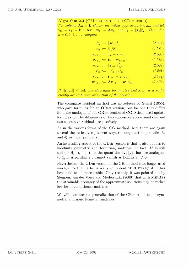
CG and Symmetric Lanczos Iterative Methods
Algorithm 2.4 (OMin form of the CR method) .For solving Ax = b choose an initial approximation x0, and letv0 := r0 := b − Ax0, w0 := Av0, and δ0 := ‖r0‖2
A. Then, forn = 0, 1, 2, . . . , compute
δ′n := ‖wn‖2 , (2.58a)
ωn := δn/δ′n , (2.58b)
xn+1 := xn + vnωn , (2.58c)
rn+1 := rn −wnωn , (2.58d)
δn+1 := ‖rn+1‖2A, (2.58e)
ψn := −δn+1/δn , (2.58f)
vn+1 := rn+1 − vnψn , (2.58g)
wn+1 := Arn+1 −wnψn . (2.58h)
If ‖rn+1‖ ≤ tol, the algorithm terminates and xn+1 is a suffi-ciently accurate approximation of the solution.
The conjugate residual method was introduces by Stiefel (1955),who gave formulas for an ORes version, but for one that differsfrom the analogue of our ORes version of CG. Stiefel used updateformulas for the differences of two successive approximations andtwo successive residuals, respectively.
As in the various forms of the CG method, here there are againseveral theoretically equivalent ways to compute the quantities δn
and δ′n as inner products.
An interesting aspect of the ODir version is that it also applies toindefinite symmetric (or Hermitian) matrices. In fact, A2 is stillspd (or Hpd), and thus the quantities ‖vn‖A2 that are analogousto δ′n in Algorithm 2.3 cannot vanish as long as vn 6= o.
Nevertheless, the ODir version of the CR method is no longer usedmuch, since the mathematically equivalent MinRes algorithm hasbeen said to be more stable. Only recently, it was pointed out bySleijpen, van der Vorst and Modersitzki (2000) that with MinResthe attainable accuracy of the approximate solutions may be ratherlow for ill-conditioned matrices.
We will later treat a generalization of the CR method to nonsym-metric and non-Hermitian matrices.
IM Script 2-14 May 20, 2008 c©M.H. Gutknecht
Iterative Methods A Bound for the Convergence
2.6 A Bound for the Convergence
For the moment, let us assume that A is symmetric and considerthe C-norm of the error vector dn, where C = A` is a positivepower of A. If A is indefinite, we need an even power to make CHpd. Then, since A = UΛU−1 with U orthogonal and Λ diagonal,and since, for any Krylov space solver, dn = pn(A)d0 according to(1.59), we have
‖dn‖C = ‖A`/2pn(A)d0‖ = ‖Upn(Λ)U−1A`/2d0‖≤ ‖pn(Λ)‖ ‖A`/2d0‖ = ‖pn(Λ)‖ ‖d0‖C= max
i=1,...,N|pn(λi)| ‖d0‖C . (2.59)
Further, we assume that the spectrum of A lies on the intervalI = [α − δ, α + δ] of the positive real axis, and we consider theChebyshev iteration for that interval. We denote its nth error vec-tor and residual polynomial by dCheb
n and pChebn , respectively, while
dn is assumed to be the error for a Krylov space solver that is op-timal in the ‖.‖C–norm of the error when applied to Ax = b witha matrix whose spectrum lies on I. Then we have
‖dn‖C‖d0‖C ≤ ‖dCheb
n ‖C‖d0‖C ≤ max
i=1,...,N|pCheb
n (λi)| ≤ minp∈Pn
p(0)=1
maxτ∈I
|p(τ)| .
(2.60)
Note that in this estimate the dependence of the residual polyno-mial on the initial residual and on the norm used is lost: we esti-mate the error of any optimal method by the error of the Chebyshevmethod, and in the estimate of the latter, the norm used has noeffect on the bound for the error reduction.
In particular, the estimate is applicable for the CG method, whichis optimal in the A–norm of the error, and for the CR method,which is optimal in the A2–norm of the error, that is, in the 2–norm of the residual.
The bound on the right-hand side of (2.60) was estimated in thederivation of Theorem 1.6.2, and we can conclude that the boundsobtained in that theorem hold here too.
Theorem 2.6.1 The residual norm reduction of the CR methodand the energy norm reduction of the CG method, when appliedto an spd system whose condition number is bounded by κI, havethe bounds given in (1.78) for the residual norm reduction of theChebyshev iteration.
c©M.H. Gutknecht May 20, 2008 IM Script 2-15
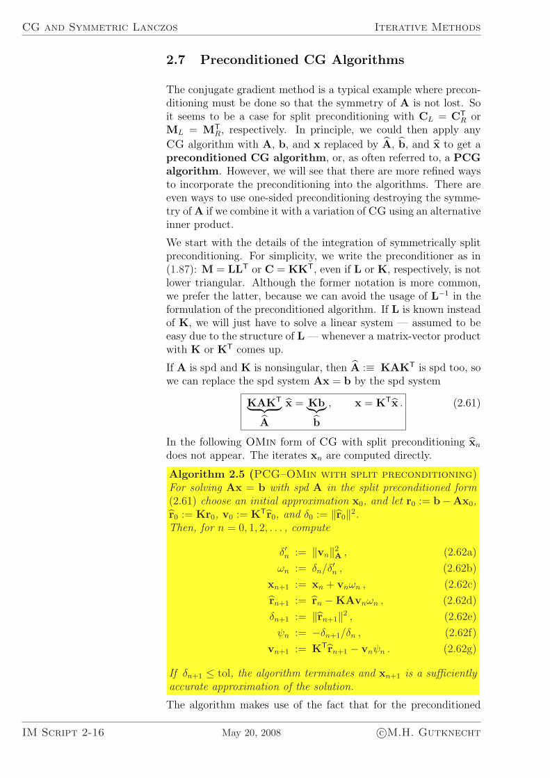
CG and Symmetric Lanczos Iterative Methods
2.7 Preconditioned CG Algorithms
The conjugate gradient method is a typical example where precon-ditioning must be done so that the symmetry of A is not lost. Soit seems to be a case for split preconditioning with CL = CT
R orML = MT
R, respectively. In principle, we could then apply any
CG algorithm with A, b, and x replaced by A, b, and x to get apreconditioned CG algorithm, or, as often referred to, a PCGalgorithm. However, we will see that there are more refined waysto incorporate the preconditioning into the algorithms. There areeven ways to use one-sided preconditioning destroying the symme-try of A if we combine it with a variation of CG using an alternativeinner product.
We start with the details of the integration of symmetrically splitpreconditioning. For simplicity, we write the preconditioner as in(1.87): M = LLT or C = KKT, even if L or K, respectively, is notlower triangular. Although the former notation is more common,we prefer the latter, because we can avoid the usage of L−1 in theformulation of the preconditioned algorithm. If L is known insteadof K, we will just have to solve a linear system — assumed to beeasy due to the structure of L — whenever a matrix-vector productwith K or KT comes up.
If A is spd and K is nonsingular, then A :≡ KAKT is spd too, sowe can replace the spd system Ax = b by the spd system
KAKT︸ ︷︷ ︸A
x = Kb︸︷︷︸b
, x = KTx . (2.61)
In the following OMin form of CG with split preconditioning xn
does not appear. The iterates xn are computed directly.
Algorithm 2.5 (PCG–OMin with split preconditioning)For solving Ax = b with spd A in the split preconditioned form(2.61) choose an initial approximation x0, and let r0 := b−Ax0,r0 := Kr0, v0 := KTr0, and δ0 := ‖r0‖2.Then, for n = 0, 1, 2, . . . , compute
δ′n := ‖vn‖2A , (2.62a)
ωn := δn/δ′n , (2.62b)
xn+1 := xn + vnωn , (2.62c)
rn+1 := rn −KAvnωn , (2.62d)
δn+1 := ‖rn+1‖2 , (2.62e)
ψn := −δn+1/δn , (2.62f)
vn+1 := KTrn+1 − vnψn . (2.62g)
If δn+1 ≤ tol, the algorithm terminates and xn+1 is a sufficientlyaccurate approximation of the solution.
The algorithm makes use of the fact that for the preconditioned
IM Script 2-16 May 20, 2008 c©M.H. Gutknecht
Iterative Methods CG and CR for complex systems
direction vectors vn :≡ K−Tvn, which do not appear, we have
‖vn‖2A
=⟨vn, Avn
⟩=
⟨K−Tvn, AK−Tvn
⟩= 〈vn,Avn〉 = ‖vn‖2
A .
Let us now turn to a widely used alternative based on precondi-tioning Ax = b on the left with the inverse M−1 of an spd matrixM that is in some sense an approximation of A. So, we solve (asin (1.83), but in different notation),
M−1A︸ ︷︷ ︸A
x = M−1b︸ ︷︷ ︸b
. (2.63)
The CG method can be defined for any inner product space, inparticular for RN with the inner product induced by M, the so-called M–inner product [M–Skalarprodukt],
〈x,y〉M :≡ 〈x,My〉 = 〈Mx,y〉 .
The matrix A :≡ M−1A in (2.63) is M–self-adjoint [M–selbst-adjungiert], that is, it is self-adjoint (or, symmetric) with respectto the M–inner product:
⟨M−1Ax,y
⟩M
= 〈Ax,y〉 = 〈x,Ay〉 =⟨x,M−1Ay
⟩M
. (2.64)
Noting that
〈rn, rn〉M = 〈rn, rn〉 ,⟨vn,M−1Avn
⟩M
= 〈vn,Avn〉
we obtain the following version of a PCG algorithm suggested byMeijerink and van der Vorst (1977):
Algorithm 2.6 (PCG–OMin with M–inner product) Forsolving Ax = b with spd A and an spd left preconditioner M as in(2.63) choose an initial approximation x0, and let r0 := b−Ax0,v0 := r0 := M−1r0, and δ0 := 〈r0, r0〉.Then, for n = 0, 1, 2, . . . , compute
δ′n := ‖vn‖2A , (2.65a)
ωn := δn/δ′n , (2.65b)
xn+1 := xn + vnωn , (2.65c)
rn+1 := rn −Avnωn , (2.65d)
rn+1 := M−1rn+1 , (2.65e)
δn+1 := 〈rn+1, rn+1〉 , (2.65f)
ψn := −δn+1/δn , (2.65g)
vn+1 := rn+1 − vnψn . (2.65h)
If δn+1 ≤ tol (or, if ‖rn+1‖2 ≤ tol), the algorithm terminates andxn+1 is a sufficiently accurate approximation of the solution.
c©M.H. Gutknecht May 20, 2008 IM Script 2-17
CG and Symmetric Lanczos Iterative Methods
2.8 CG and CR for Complex Systems
The CG and CR methods can also be applied to linear systemsAx = b with complex data A and b, but again, for CG the matrixmust be Hermitian positive definite (Hpd), and for CR it must beHermitian. Of course, in the formulas AT has to be replaced byAH, and 〈x,y〉 :≡ xTy becomes2 〈x,y〉 :≡ xHy.
Some adaptations are necessary in the treatment of error functionalminimization: In particular, in (2.1) bTx is replaced by Re (bHx) =Re 〈b,x〉, and in (2.52) we have Re (bHAx) = Re 〈b,Ax〉.With these changes, virtually everything remains correct.
In the following we normally allow that the data are complex, al-though in nearly all applications they are real. Recall that we letE :≡ R or C to combine the real and the complex cases, and thatwe denote the adjoint of A by A? — so this is the transpose AT ifA is real, and the Hermitian transpose AH if A is complex.
2.9 CG for Least Squares Problems
When parameters of a linear model are determined by measure-ments, the influence of measurement errors can be reduced by mak-ing many more measurements than the number of parameters. Thisleads to an overdetermined linear system Ax ≈ b of M equa-tions in N unknowns, where M > N .
The classical approach to this problem, introduced by Gauss, is todetermine the approximate solution for which the (Euclidean) 2-norm of the residual is minimized, or, what amounts to the same,where the square of this 2-norm is minimized:
‖r‖2 = ‖b−Ax‖2 = min! (2.66)
Since ‖r‖2 =∑
r2i , Gauss called this approximation the least
squares solution. The geometric properties of the Euclideanspace imply that the residual of the least squares solution is or-thogonal to the column space of A, so A?r = o or
A?Ax = A?b . (2.67)
These are the normal equations. We assume that A has fullcolumn rank (i.e., rankA = N). Then A?A is Hpd and the CGmethod can be applied to the normal equations (2.67). This ap-proach is known as the CGNR method; the “N” and “R” refer tothe normal equations and the residual, respectively. It means thatthe approximate solutions are chosen such that
xn − x0 ∈ Kn(A?A,A?r0) , where r0 :≡ b−Ax0 . (2.68)
2Attention: many mathematicians define 〈x,y〉 :≡ yHx instead.
IM Script 2-18 May 20, 2008 c©M.H. Gutknecht
Iterative Methods CG for Least Squares Problems
Hence, with B :≡ AA?, the residuals rn :≡ b−Axn satisfy
rn − r0 ∈ AKn(A?A,A?r0) = AA?Kn(AA?, r0) = BKn(B, r0) .
(2.69)
Applying CG to the normal equations means that the residualssn :≡ A?rn of the normal equations are orthogonal, so they satisfy
sn − s0 ∈ A?AKn(A?A, s0) , sn ⊥ Kn(A?A, s0) . (2.70)
It follows that for the residuals rn = b−Axn of the given systemholds the Galerkin condition
rn ⊥ AKn(A?A,A?r0) = BKn(B, r0) . (2.71)
Let us summarize some of these results:
Theorem 2.9.1 Let a full rank overdetermined rectangular sys-tem Ax = b be given; so A is M × N , rankA = N ≤ M . Itsleast squares solution minimizing (2.66) is the unique solution ofthe normal equations (2.67).The CGNR method consisting of applying the CG method to thesenormal equations has the following properties:
• The iterates xn minimize the 2-norm of the residuals rn :≡b − Axn of the original system subject to the condition(2.68), and in this sense they are least squares solution ofthe given system restricted further by (2.68).
• The residuals rn satisfy (2.69) and (2.71). For the residualssn of the normal equations holds (2.70).
On the other hand, if the given system Ax = b is an underde-termined linear system of M equations in N unknowns, whereM < N , then we can restrict x to the image of A? in order to definea unique solution if A has full rank M , which we assume again. Wedefine z by
x ≡: A?z (2.72)
and write the given system as
AA?z = b , (2.73)
which is again referred to as normal equations. We claim that(2.72) restricts x to be orthogonal to the nullspace (or, kernel) ofA. In fact, we can write any x′ ∈ EN as
x′ = x⊥ + A?z , where x⊥ ⊥ imA? , z ∈ EM . (2.74)
The latter means that⟨x⊥,A?w
⟩= 0 (∀w ∈ EM) or Ax⊥ ⊥ EM ,
which implies that Ax⊥ = o. In other words, x⊥ lies in the kernelof A. Actually, it is a well-known fact from matrix theory thatthe kernel (or null space) of A and the image (or range) of A? are
c©M.H. Gutknecht May 20, 2008 IM Script 2-19
CG and Symmetric Lanczos Iterative Methods
orthogonal complementary subspaces. We conclude that Ax′ =AA?z. So any solution of the given system Ax′ = b has the form(2.74) with z = z being a solution of (2.73) and x⊥ ∈ ker A. FromPythagoras’ theorem we can conclude further that
‖x′‖2 = ‖x⊥‖2 + ‖A?z‖2 .
Hence, x = A?z is the shortest solution. In other words, if A hasfull rank M (< N), then under the substitution x = A?z the system(2.73) is equivalent with
Ax = b , ‖x‖ = min! (2.75)
Since AA? is Hpd, we can apply CG to the normal equations (2.73).This is the CGNE method, where “E” now refers to the error. Itis also called Craig’s method. If zn is any approximate solution,the corresponding residual is
‖rn‖ = ‖b−AA?zn‖ = ‖b−Axn‖ (2.76)
and is also the residual of the original system. So, implicitly, CGNEyields approximate solutions zn of the normal equations (2.73) with
zn − z0 ∈ Kn(AA?, r0) = Kn(B, r0) , (2.77)
corresponding approximate solutions of the original system with
xn − x0 ∈ A?Kn(AA?, r0) = Kn(A?A,A?r0) , (2.78)
as well as residuals that satisfy again (2.69) and, as can be seen,
rn ⊥ Kn(AA?, r0) = Kn(B, r0) . (2.79)
Consequently, the relevant Krylov space is the same as for CGNR,but the Galerkin condition is different.
In the nth step, the AA?-norm or B-norm of the error zn−(AA?)−1bof (2.73) is minimized subject to the condition (2.77). This is thesame as minimizing the 2-norm of the error xn − x? of the originalsystem subject to the condition (2.78).
IM Script 2-20 May 20, 2008 c©M.H. Gutknecht
Iterative Methods CG for Least Squares Problems
Theorem 2.9.2 Let a full rank underdetermined rectangular sys-tem Ax = b be given; so A is M × N , rankA = M < N .Its least squares solution minimizing (2.75) is the unique solu-tion of the normal equations (2.73). Any other solution is of theform x = x⊥ + A?z, where x⊥ ⊥ imA?, which is equivalent tox⊥ ∈ ker A.The CGNE algorithm consisting of applying the CG method tothese normal equations has the following properties:
• zn minimizes the B-norm of the error of the normal equa-tions (2.73) subject to (2.77), where B :≡ AA?.
• The corresponding original approximations xn = A?zn min-imize the 2-norm of the errors xn−x? of the original systemsubject to the condition (2.78).
• The residuals rn, which are both the residuals of the origi-nal system and the normal equations, satisfy (2.69) (as inCGNR) and the Galerkin condition (2.79).
The theorem remains correct for M = N if we let x⊥ := o. Thecondition ‖x‖ = min! in (2.75) can be dropped because Ax = bhas then a unique solution.
Let us now look at the normally used OMin algorithms of theCGNR and CGNE methods. We have to adapt Algorithm 2.1 ofSection 2.4 so that it is applied to the normal equations (2.67) and(2.73), respectively.
For CGNR the relevant residuals that are orthogonal to each otherare the residuals sn(= A?r0) of the normal equations that satisfy(2.70). They also determine δn. The search directions vn are nowA?A-orthogonal, and thus δ′n := ‖vn‖2
A?A = ‖Avn‖2.
Algorithm 2.7 (OMin form of the CGNR method) .For solving the least squares problem (2.66) via the normal equa-tions (2.67) choose an initial approximation x0, and let r0 :=b−Ax0, v0 := s0 := A?r0, δ0 := ‖s0‖2, and ψ−1 := 0. Then, forn = 0, 1, 2, . . . , compute
δ′n := ‖Avn‖2 , (2.80a)
ωn := δn/δ′n , (2.80b)
xn+1 := xn + vnωn , (2.80c)
rn+1 := rn −Avnωn , (2.80d)
sn+1 := A?rn+1 , (2.80e)
δn+1 := ‖sn+1‖2 , (2.80f)
ψn := − δn+1/δn , (2.80g)
vn+1 := sn+1 − vnψn . (2.80h)
If ‖rn+1‖ ≤ tol, the algorithm terminates and xn+1 is a suffi-ciently accurate approximation of the solution.
c©M.H. Gutknecht May 20, 2008 IM Script 2-21
CG and Symmetric Lanczos Iterative Methods
We have chosen to update in (2.80d) also rn, which allows us torely on ‖rn+1‖ for termination. One could instead update directlysn according to
sn+1 := sn −A?Avnωn , (2.81)
but then termination must rely on ‖sn+1‖.For CGNE the residuals rn are the same for the original and thenormal equations (2.73), but the iterates seem to change to zn.However, it turns out that instead everything can be formulatedin terms of the approximate solutions xn = A?zn of the originalsystem and the corresponding search directions.
Algorithm 2.8 (OMin form of the CGNE method) .For solving the minimum solution least squares problem (2.75) viathe normal equations (2.73) choose an initial approximation x0,and let v0 := r0 := b−Ax0, δ0 := ‖r0‖2, and ψ−1 := 0.Then, for n = 0, 1, 2, . . . , compute
δ′n := ‖vn‖2 , (2.82a)
ωn := δn/δ′n , (2.82b)
xn+1 := xn + vnωn , (2.82c)
rn+1 := rn −Avnωn , (2.82d)
δn+1 := ‖rn+1‖2 , (2.82e)
ψn := − δn+1/δn , (2.82f)
vn+1 := A?rn+1 − vnψn . (2.82g)
If ‖rn+1‖ ≤ tol, the algorithm terminates and xn+1 is a suffi-ciently accurate approximation of the solution.
A potential disadvantage of using the normal equations (2.67) and(2.73) is that the condition number of A?A and AA? may be largecompared to the one of the triangular matrix R in a QR decompo-sition of A. In particular, if A is square and nonsingular,
κ2(A?A) = κ2(AA?) = (κ2(A))2 = (κ2(R))2 .
IM Script 2-22 May 20, 2008 c©M.H. Gutknecht
Iterative Methods References
Bibliography
W. E. Arnoldi (1951), ‘The principle of minimized iterations in the solu-tion of the matrix eigenvalue problem’, Quart. Appl. Math. 9, 17–29.
S. F. Ashby, T. A. Manteuffel and P. E. Saylor (1990), ‘A taxonomyfor conjugate gradient methods’, SIAM J. Numer. Anal. 27, 1542–1568.
J. K. Cullum and R. A. Willoughby (1985), Lanczos Algorithms forLarge Symmetric Eigenvalue Computations (2 Vols.), Birkhauser,Boston-Basel-Stuttgart.
J. Dongarra and F. Sullivan (2000), ‘Guest editors’ introduction to thetop 10 algorithms’, Computing in Science and Engineering 2(1), 22–23.
B. Fischer and R. W. Freund (1990), ‘On the constrained Chebyshev ap-proximation problem on ellipses’, Journal of Approximation Theory62, 297–315.
B. Fischer and R. W. Freund (1991), ‘Chebyshev polynomials are notalways optimal’, Journal of Approximation Theory 65, 261–272.
R. Fletcher (1976), Conjugate gradient methods for indefinite systems,in Numerical Analysis, Dundee, 1975 (G. A. Watson, ed.), Vol. 506of Lecture Notes in Mathematics, Springer, Berlin, pp. 73–89.
R. W. Freund and N. M. Nachtigal (1991), ‘QMR: a quasi-minimalresidual method for non-Hermitian linear systems’, Numer. Math.60, 315–339. Received Feb. 19, 1991.
G. H. Golub and R. S. Varga (1961), ‘Chebyshev semiiterative meth-ods, successive overrelaxation iterative methods, and second orderRichardson iterative methods’, Numer. Math. 3, 147–168.
A. Greenbaum (1997), Iterative Methods for Solving Linear Systems,SIAM, Philadelphia, PA.
P. Henrici (1974), Applied and Computational Complex Analysis, Vol.1, Wiley, New York.
M. R. Hestenes and E. Stiefel (1952), ‘Methods of conjugate gradients forsolving linear systems’, J. Res. Nat. Bureau Standards 49, 409–435.
R. A. Horn and C. R. Johnson (1985), Matrix Analysis, CambridgeUniversity Press, New York.
c©M.H. Gutknecht May 20, 2008 IM Script Refs.-1
References Iterative Methods
C. Lanczos (1950), ‘An iteration method for the solution of the eigen-value problem of linear differential and integral operators’, J. Res.Nat. Bureau Standards 45, 255–281.
C. Lanczos (1952), ‘Solution of systems of linear equations by minimizediterations’, J. Res. Nat. Bureau Standards 49, 33–53.
J. A. Meijerink and H. A. van der Vorst (1977), ‘An iterative solutionmethod for linear equations systems of which the coefficient matrixis a symmetric M-matrix’, Math. Comp. 31, 148–162.
C. C. Paige (1971), The computations of eigenvalues and eigenvectorsof very large sparse matrices, PhD thesis, University of London.
C. C. Paige and M. A. Saunders (1975), ‘Solution of sparse indefinitesystems of linear equations’, SIAM J. Numer. Anal. 12, 617–629.
B. N. Parlett (1980), The Symmetric Eigenvalue Problem, Prentice-Hall,Englewood Cliffs, N.J.
H. Rutishauser (1957), Der Quotienten-Differenzen-Algorithmus, Mitt.Inst. angew. Math. ETH, Nr. 7, Birkhauser, Basel.
H. Rutishauser (1959), Theory of gradient methods, in Refined IterativeMethods for Computation of the Solution and the Eigenvalues ofSelf-Adjoint Boundary Value Problems, Mitt. Inst. angew. Math.ETH Zurich, Nr. 8, Birkhauser, Basel, pp. 24–49.
Y. Saad (1996), Iterative Methods for Sparse Linear Systems, PWS Pub-lishing, Boston.
Y. Saad and M. H. Schultz (1985), ‘Conjugate gradient-like algorithmsfor solving nonsymmetric linear systems’, Math. Comp. 44, 417–424.
O. Schenk (2000), Scalable Parallel Sparse LU Factorization Methodson Shared Memory Multiprocessors, PhD thesis, Diss. No. 13515,ETH Zurich, Zurich, Switzerland.
H. R. Schwarz, H. Rutishauser and E. Stiefel (1968), Numerik sym-metrischer Matrizen, Teubner, Stuttgart.
G. L. G. Sleijpen, H. A. van der Vorst and J. Modersitzki (2000),‘Differences in the effects of rounding errors in Krylov solvers forsymmetric indefinite linear systems’, SIAM J. Matrix Anal. Appl.22(3), 726–751.
E. Stiefel (1955), ‘Relaxationsmethoden bester Strategie zur Losung lin-earer Gleichungssysteme’, Comm. Math. Helv. 29, 157–179.
G. Strang (1986), Introduction to Applied Mathematics, Wellesley–Cambridge Press, Wellesley, MA, U.S.A.
H. A. van der Vorst (2000), ‘Krylov subspace iteration’, Computing inScience and Engineering 2, 32–37.
R. S. Varga (1962), Matrix Iterative Analysis, Prentice-Hall, EnglewoodCliffs, N.J. Rev. 2nd ed., Springer-Verlag, 1999.
IM Script Refs.-2 May 20, 2008 c©M.H. Gutknecht

Iterative Methods References
H. F. Walker and L. Zhou (1994), ‘A simpler GMRES’, Numer. LinearAlgebra Appl. 1(6), 571–581.
D. M. Young (1950), Iterative Methods for Solving Partial Differ-ence Equations of Elliptic Type, PhD thesis, Harvard University.http://www.cs.utexas.edu/users/young/david young thesis.pdf.
D. M. Young (1971), Iterative Solution of Large Linear Systems, Aca-demic Press, Orlando.
c©M.H. Gutknecht May 20, 2008 IM Script Refs.-3
Index
E, 1-4M–Skalarprodukt, 2-17M–inner product, 2-17M–selbst-adjungiert, 2-17M–self-adjoint, 2-17aussere Iteration, 1-31CGNE method
OMin form, 2-22CGNR method
OMin form, 2-21CG method, 2-5
ODir form, 2-11OMin form, 2-7ORes form, 2-11convergence bound, 2-15coupled two-term version, 2-7Hestenes-Stiefel algorithm, 2-7preconditioned, 2-16three-term version, 2-11
CR method, 2-13OMin form, 2-13convergence bound, 2-15
ODir form of CG, 2-11OMin form of CG, 2-7OMin form of CGNE, 2-22OMin form of CGNR, 2-21OMin form of CR, 2-13OMin form of PCG
with split preconditioning, 2-16with with M–inner product, 2-17
ORes form of CG, 2-7, 2-11PCG algorithm, 2-16PCG method
OMin form with split preconditioning,2-16
OMin form with with M–inner product,2-17
CGNE method, 2-20CGNR method, 2-18
approximate inverse, 1-26approximative Inverse, 1-26
Caley-Hamilton theorem, 1-16Chebyshev iteration, 1-20, 1-22, 1-23
Chebyshev polynomial, 1-21shifted and scaled, 1-21
Chebyshev semi-iterative method, 1-22Cholesky decomposition, 1-27Cholesky factorization
incomplete, 1-29Cholesky-Zerlegung, 1-27
unvollstandige, 1-29compatible norm, 1-7conjugate direction, 2-3conjugate direction method, 2-4conjugate gradient method, 2-5conjugate residual (CR) method, 2-13consistency condition
polynomial version, 1-18consistently ordered, 1-12contraction, 1-6convergence bound, 2-15convergence factor
asymptotic, 1-25Craig’s method, 2-20
dunn besetzte Matrix, 1-1dunn besetztes lineares Gleichungssystem,
1-1dunn besetztes Matrix-Eigenwertproblem,
1-1damped Jacobi iteration, 1-11direct method, 1-5direction
conjugate, 2-3of steepest descent, 2-2
direction vector, 2-3
Eigenwert-Zerlegung, 1-6eigenvalue decomposition, 1-6Einzelschrittverfahren, 1-10Energienorm, 2-1energy norm, 2-1error (vector), 1-9error vector
preconditioned, 1-27
Fehler(vektor), 1-9fill-in, 1-5, 1-29
Index-1
Index Iterative Methods
finite termination property, 1-17fixed point iteration, 1-6Fixpunkt-Iteration, 1-6flexible preconditioning, 1-31flexible Vorkonditionierung, 1-31
Gauss-Seidel method, 1-10Gauss-Seidel-Verfahren, 1-10gedampftes Gesamtschritt-Verfahren, 1-11Grad, 1-14grade, 1-14
Hestenes-Stiefel algorithm, 2-7Hpd, 1-4, 1-20, 2-18
IC factorization, 1-29ILU factorization, 1-29ILUT, 1-30incomplete Cholesky (IC) factorization, 1-29incomplete LU (ILU) factorization, 1-29inner iteration, 1-31inner-outer iteration, 1-31innere Iteration, 1-31Inverse
approximative, 1-26inverse
approximate, 1-26iterate, 1-6Iterierte, 1-6
Jacobi iteration, 1-6, 1-10damped, 1-11
Jacobi overrelaxation (JOR) method, 1-11JOR, 1-11Jordan block, 1-6Jordan canonical form, 1-6Jordansche Normalform, 1-6Jordanscher Block, 1-6Joukowski transformation, 1-24
kompatible Norm, 1-7konjugierte Richtung, 2-3konsistent geordnet, 1-12Konsistenz-Bedingung, 1-18Kontraktion, 1-6Krylov (sub)space, 1-14Krylov basis, 1-17Krylov space method
(standard), 1-18nonstandard, 1-18
Krylov space solver(standard), 1-18
Krylov subspace method, 1-18Krylov-Raum-Methode
(Standard-), 1-18Nicht-Standard, 1-18
Krylovbasis, 1-17
least squares solution, 2-18line search, 2-2linear system
overdetermined, 2-18underdetermined, 2-19
LU decomposition, 1-5LU factorization, 1-5
incomplete, 1-29LU-Zerlegung
unvollstandige, 1-29
M-Matrix, 1-13M-matrix, 1-13Matrix
dunn besetzt, 1-1matrix
sparse, 1-1matrix splitting, 1-13matrix-vector multiplication (MV), 1-2Matrix-Vektor-Multiplikation, 1-2method
of conjugate directions, 2-4of conjugate residuals, 2-13
method of steepest descent, 2-2Methode
der konjugierten Gradienten, 2-5Methode der konjugierten Residuen, 2-13Methode der konjugierten Richtungen, 2-4Methode des steilsten Abstiegs, 2-2minimal polynomial, 1-15Minimalpolynom, 1-15Muster, 1-29MV, 1-2
normcompatible, 1-7energy, 2-1
normal equations, 2-18, 2-19
outer iteration, 1-31overdetermined linear system, 2-18
pattern, 1-29Picard iteration, 1-6Poisson problem, 1-3polynomial preconditioner, 1-31polynomialer Prakonditionierer, 1-31Prakonditionierer
polynomialer, 1-31Prakonditionierung, 1-26
IM Script Index-2 May 20, 2008 c©M.H. Gutknecht
Iterative Methods Index
preconditionerleft, 1-26polynomial, 1-31right, 1-26split, 1-27
preconditioning, 1-26flexible, 1-31left, 1-26right, 1-26split, 1-26
Property A, 1-12
quotient-difference (qd) algorithm, 2-12
R-factor, 1-7recursion
three-termstationary, 1-25
recursionsthree-term, 2-10
red-black ordering, 1-4regulares Splitting, 1-13regular splitting, 1-13Relaxation, 1-11relaxation, 1-11relaxation factor, 1-11Relaxationsfaktor, 1-11residual (vector), 1-9residual polynomial, 1-18residual vector
preconditioned, 1-27Residualpolynom, 1-18Residuenvektor, 1-9Residuum, 1-9Richardson iteration
non-stationary, 1-11second-order, 1-25stationary, 1-11
Richtungkonjugiert, 2-3
Richtungsvektor, 2-3root-convergence factor
asymptotic, 1-25root-convergence factor, 1-7
search direction, 2-3second-order Richardson iteration, 1-25SOR method, 1-12
symmetric, 1-12sparse direct method, 1-5sparse direct solver, 1-5sparse linear system of equations, 1-1sparse matrix, 1-1
sparse matrix eigenvalue problem, 1-1spd, 1-4, 1-20spectral radius, 1-6stationary Richardson iteration, 1-11steepest descent, 2-2step size
optimal, 2-4successive overrelaxation (SOR) method,
1-12Suchrichtung, 2-3sweep, 1-10symmetric SOR (SSOR) method, 1-12
Tschebyscheff–Polynom, 1-21Tschebyscheff-Iteration, 1-22
underdetermined linear system, 2-19unvollstandige Cholesky-Zerlegung, 1-29unvollstandige LU-Zerlegung, 1-29
Verfahren der sukzessiven Uberrelaxation,1-12
Vorkonditionierergesplitteter, 1-27linker, 1-26rechter, 1-26
Vorkonditionierung, 1-26flexible, 1-31gesplittete, 1-26linke, 1-26rechte, 1-26
Wurzel-Konvergenzfaktor, 1-7
c©M.H. Gutknecht May 20, 2008 IM Script Index-3


