Iterative Numerical Methods for Real Eigenvalues and Eigenvectors of Matrices John Coffey, Cheshire, UK. August 2016 Key words: matrix, eigenvalue, eigenvector, iteration, power method, inverse power method, shifting, Rayleigh quotient, LU decomposition, matrix deflation, rank order reduction, QR, Schur decomposition, geometric series, Jacobi method, Hessenberg matrix, Householder reflector, Francis’ implicitly shifted QR algorithms. 1 Introduction This article gives a brief, informal account of some aspects of iterative numerical methods for finding the real eigenvalues and eigenvectors of square matrices with real elements. There is a large, well documented literature on this subject and many computer algorithms and sophisticated programs to implement them. The whole subject is interesting because of the innovative methods that have been devised to persuade matrices to reveal their eigen pairs (values and vectors). This article touches on only a few aspects which I have looked at for personal interest, my aim being to remind myself of the properties of matrices and thence to gain some understanding of the numerical techniques which have been developed. I came to this subject through the modelling of vibrating structures using finite element methods. In these the structure is represented by elastic elements defined over a mesh of nodes, and the mass and stiffness are represented by symmetric matrices M and K respectively. In a previous article on www.mathstudio.co.uk entitled ‘Periodic Forced Vibrations, Normal Modes and Damping, with Measurements on a ’Cello’ I explain how the equations of motion can be written in the form Kx =-ω 2 Mx or M -1 Kx = ω 2 x . (1) This is a linear eigenvalue problem with the standard form Ep = λp where the natural frequencies of vibration are given by the square roots of the eigenvalues λ = ω 2 . The corresponding eigenvectors p give the relative amplitudes of motion at the mesh nodes. When these calculations are carried out by finite element programs, the eigenvalue/eigenvector pairs are determined to chosen precision by iterative numerical methods. This contrasts with the approach in analytical mathematics where the steps are as follows: 1. Let the n × n square matrix be E and let I be the unit matrix of the same dimension. Form E - λI where λ is a scalar to be determined. 2. Evaluate the determinant of E - λI. This will be a polynomial in λ of degree n. Solve for the n zeros, which may be real and distinct, real with multiplicity or in complex conjugate pairs. These are the eigenvalues λ 1 , λ 2 , ... λ n . 1
Transcript
Iterative Numerical Methods for Real
Eigenvalues and Eigenvectors of Matrices
John Coffey, Cheshire, UK.
August 2016
Key words: matrix, eigenvalue, eigenvector, iteration, power method, inverse power method,shifting, Rayleigh quotient, LU decomposition, matrix deflation, rank order reduction, QR, Schur
This article gives a brief, informal account of some aspects of iterative numerical methods for findingthe real eigenvalues and eigenvectors of square matrices with real elements. There is a large, welldocumented literature on this subject and many computer algorithms and sophisticated programs toimplement them. The whole subject is interesting because of the innovative methods that have beendevised to persuade matrices to reveal their eigen pairs (values and vectors). This article touches ononly a few aspects which I have looked at for personal interest, my aim being to remind myself ofthe properties of matrices and thence to gain some understanding of the numerical techniques whichhave been developed.
I came to this subject through the modelling of vibrating structures using finite elementmethods. In these the structure is represented by elastic elements defined over a mesh of nodes, andthe mass and stiffness are represented by symmetric matrices M and K respectively. In a previousarticle on www.mathstudio.co.uk entitled ‘Periodic Forced Vibrations, Normal Modes and Damping,with Measurements on a ’Cello’ I explain how the equations of motion can be written in the form
Kx = −ω2Mx or M−1Kx = ω2x . (1)
This is a linear eigenvalue problem with the standard form Ep = λp where the natural frequenciesof vibration are given by the square roots of the eigenvalues λ = ω2. The corresponding eigenvectorsp give the relative amplitudes of motion at the mesh nodes. When these calculations are carried outby finite element programs, the eigenvalue/eigenvector pairs are determined to chosen precision byiterative numerical methods. This contrasts with the approach in analytical mathematics where thesteps are as follows:
1. Let the n × n square matrix be E and let I be the unit matrix of the same dimension. FormE − λI where λ is a scalar to be determined.
2. Evaluate the determinant of E − λI. This will be a polynomial in λ of degree n. Solve for then zeros, which may be real and distinct, real with multiplicity or in complex conjugate pairs.These are the eigenvalues λ1, λ2, ... λn.
1
3. To find the corresponding eigenvectors, substitute λj into E − λI = 0. The result will bea singular matrix which represents the coefficients of a set of simultaneous equations in thecomponents of the eigenvector pj . Take one of these components to have a given value (usually1) and solve for the other n − 1 components. This can be done by inverting the n − 1 by n − 1matrix obtained by deleting the row and column indexed by the chosen component.
This procedure is of wide applicability and would in principle give the exact eigenvalues andeigenvectors provided arbitrary precision arithmetic were used. It applies equally to real matriceswith real eigenvalues, ones with some complex conjugate eigenvalue pairs, and to matrices withcomplex elements. However, in practice it is only applicable to relatively small matrices – say up to10×10. The effort in evaluating the determinant, solving numerically for all n roots, and then solvingthe set of n − 1 simultaneous equations is prohibitive for large matrices and rounding errors becometroublesome. Bear in mind that some matrices in finite element calculations may have thousandsof elements, making computer storage an issue even today. To avoid the obstacles to computationin the direct approach, several iterative numerical schemes have been developed over many years.There are three main computational challenges:
� to find all the eigenvalues and eigenvectors, or at least all of interest. In vibration problemsoften the eigenvalues with smallest magnitude are most important because they correspond tothe lowest frequencies,
� for any identified eigenvalue, to converge rapidly and accurately,
� for any identified eigenvector, to converge rapidly and accurately. Some methods converge onboth an eigenvector its eigenvalue simultaneously.
I deal entirely with real square matrices, and most examples will have only real eigenvalues.I describe some of the basic methods, commenting on convergence rates and applicability, but thereis no deep analysis of stability or the computational effort required. Though these matter are centralto numerical analysis, the reader must look to the literature for such details. Four books which givethorough accounts of this large subject are
� ‘The Algebraic Eigenvalue Problem’ by J. H. Wilkinson, Oxford Univ, Press, 1965
� ‘Matrix Computations’ by Gene H. Golub and Charles F. Van Loan, Third Edn. 1996, JohnHopkins Univ Press. Available electronically on the internet.
� ‘The Matrix Eigenvalue Problem: GR and Krylov Subspace Methods’ by David S. Watkins,pub. SIAM, 2007
� ‘Fundamentals of Matrix Computations’ by David S. Watkins, Third Edn. 2010. Pub. JohnWiley.
There are also many original papers and lecture notes on the internet, including the review of theQR algorithm 50 years on by Gene Golub and Frank Uhlig1.
In this article the scene is set in §2 by listing some useful properties of matrices and theireigenvalues and eigenvectors and giving numerical illustrations in §3. The similarity transformationis perhaps the most important concept because it changes the matrix to a more tractable formwithout changing its eigenvalues. The next two sections are all related to the Power Method by
1 IMA Journal of Numerical Analysis Vol 29, 467-485, 2009.
2
which the dominant eigenvalue (the one with largest absolute value) and its eigenvector are foundsimultaneously. §4 describes the basic, direct power method with an example. Shifting the diagonalof the matrix by subtracting a constant can lead to faster convergence since the rate depends onthe ratio of eigenvalues. §5 explains how fast convergence can be obtained with the inverse powermethod, and how the direct power and inverse power methods can be use together to find one eigenpair at a time. The inverse method in principle involves the inverse of the given matrix, but theproblems in actually finding the inverse are in practice circumvented by the equivalent process ofsolving a system of simultaneous equations, and this in turn is made straightforward by factorisingthe given matrix into a product LU of a lower (L) and an upper (U) triangular matrix.
After the dominant and possibly one or two other eigen pairs have been found, ‘matrixdeflation’ may be used to allow more to be found. Deflation means finding a smaller matrix whichhas the same eigenvalues and vectors as the given matrix expect for one or two known eigen pairswhich have been removed. It is a way of chopping off the eigen pairs which have already beendetermined from the matrix, allowing further calculation of the dominant eigenpairs in the reducedmatrix which has smaller eigenvalues. Some deflation and matrix order reduction algorithms aredescribed in §6.
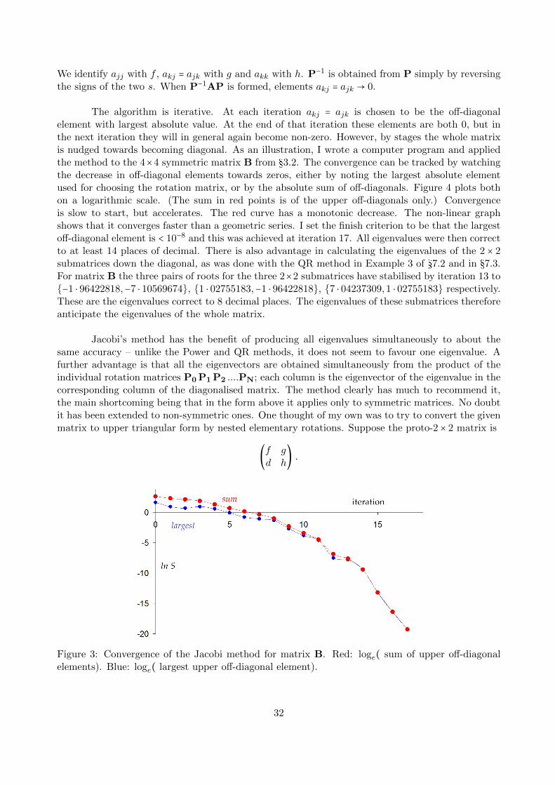
§7 deals with an algorithm first described by Carl Jacobi in 1841. Though this is effective onlyfor symmetric matrices, it has the attractive property of converging on all eigenvalues simultaneously,in contrast with the power method. It is probably the earliest method with this property. Jacobi’smethod works through a sequence of nested similarity transformations at each of which one pair ofthe elements in the lower left and upper right of the matrix is mapped to 0 by, in effect, a rotationof axes. In this way the matrix is gradually transformed to a diagonal matrix where the eigenvaluescan be read down the diagonal.
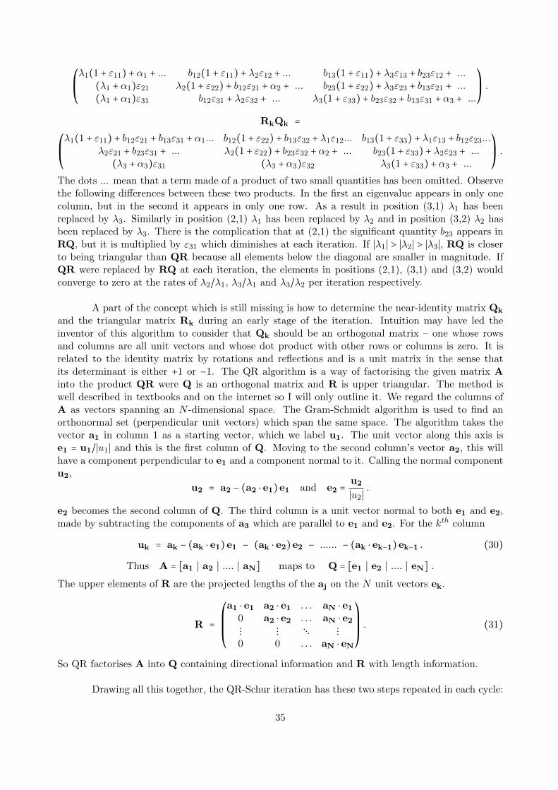
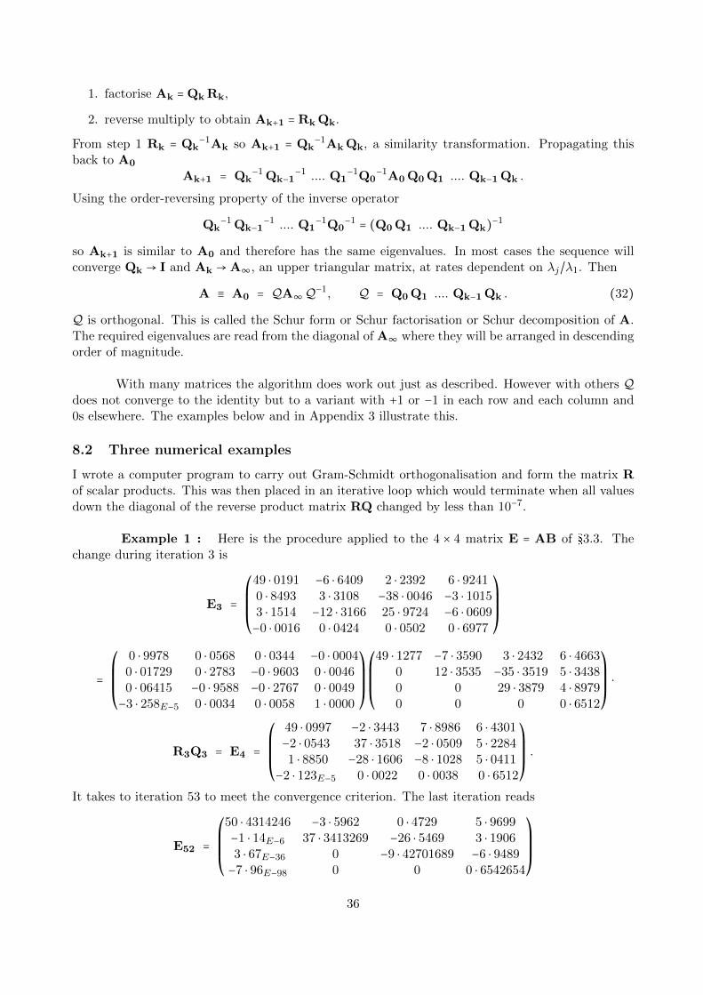
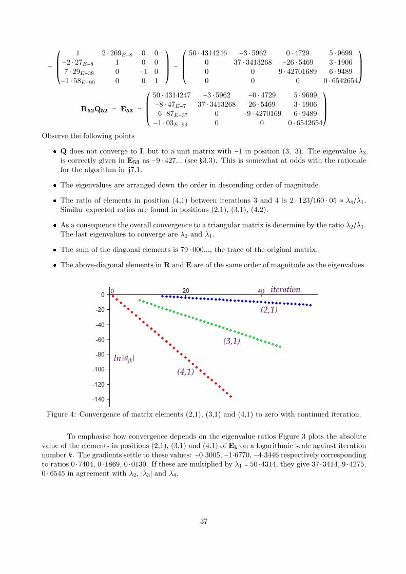
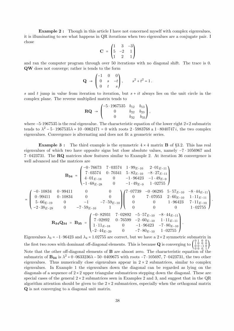
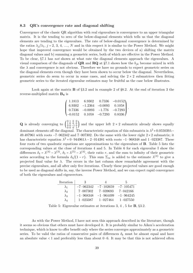
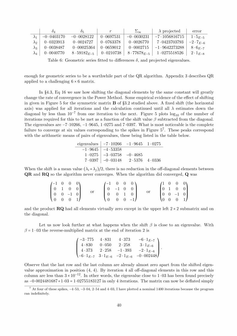
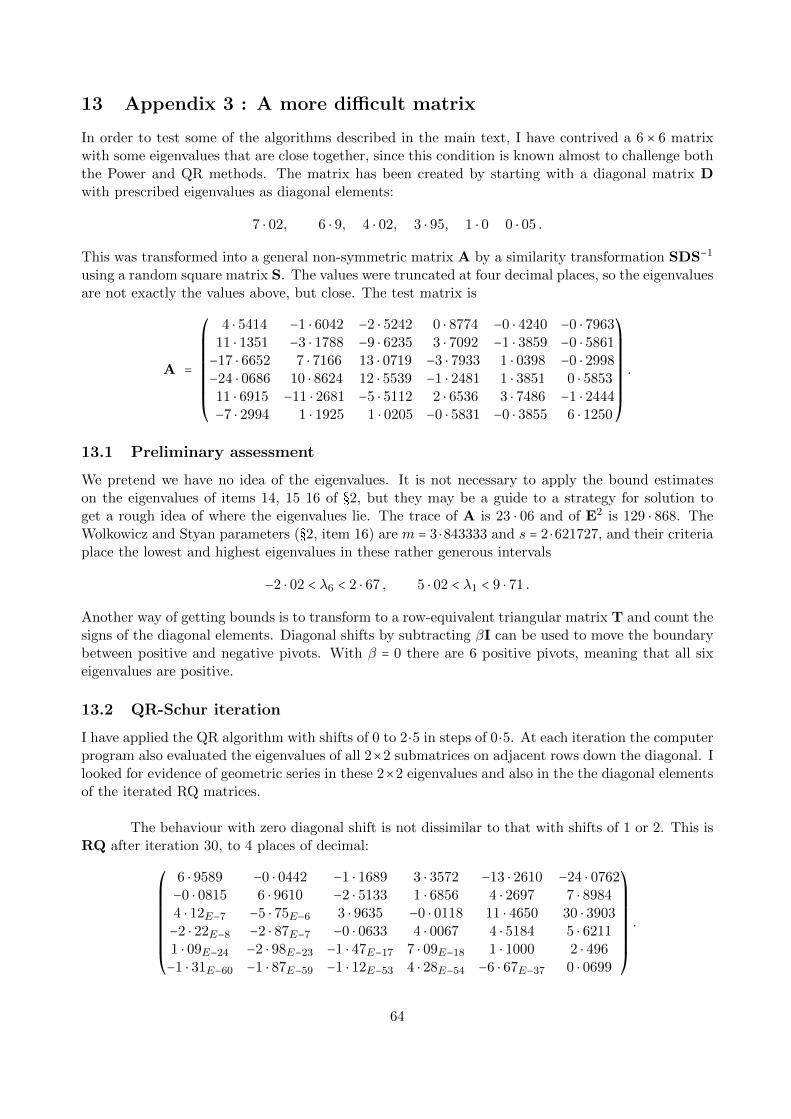
§8 returns to the idea of factorising a matrix into a product of two with special properties.Historically, the LU decomposition described in §5 was extended by Heinz Rutishauser in the late1950s into an iterative algorithm called LR. This had serious stability problems for some types ofmatrix, but the idea was sound and was part of the inspiration of John Francis in Britain andVera Kublanovskaya in Russia to develop the more stable QR method in about 1960. The basicor ‘explicit’ QR method is described with examples in §8. At each stage of iteration the startingmatrix A is factored into the product QR where Q is an orthogonal matrix, found by the Gram-Schmidt procedure, and R is upper triangular, the so-called Schur equivalent form of A. Thesefactors are then multiplied in reverse order RQ which happens to have smaller elements below themain diagonal. After several iterations RQ is itself almost triangular, at which stage the all theeigenvalues can be read down the diagonal.
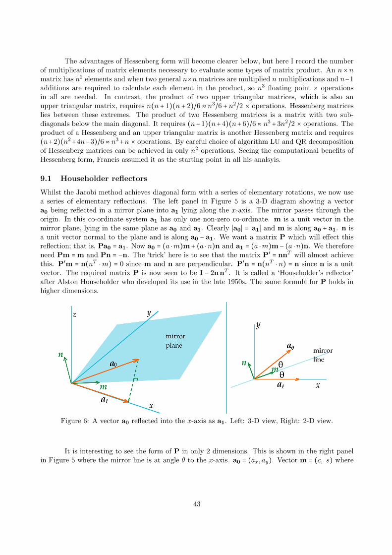
John Francis published two seminal papers in 1960 and 1961 respectively. In the second hedeveloped modifications of the QR method which were so profound that they constitute a distinctand powerful algorithm which has since been known as the ‘implicitly shifted QR algorithm’. Inrecent years David Watkins of Washington State University, who has written extensively on thesubject, has urged that it be renamed ‘Francis’s algorithm’, pointing out that it is better understoodin its own right rather than as a version of the basic QR algorithm. Francis’ algorithm requires firstthat the given matrix be put into so-called Hessenberg form in which all elements below the sub-diagonal (lower off-diagonal) are zero. Methods for transforming to Hessenberg form using matricesequivalent to reflections are described in §9. Francis’ single and double shift algorithms are outlinedin §10.
3
Paradoxically, though my interest was stimulated by eigenvalue solutions of finite elementmodels, I do not say much in this article about the numerical methods most suited to the large,sparse matrices which typically arise with finite elements. Very large matrices are best not storedin a computer as n × n arrays in which almost all elements are zero, but rather as a list of thenon-zero elements together with their two positional indices. Several of the more powerful numericalmethods for general, dense matrices, such as the QR family of algorithms, involve matrix-by-matrixmultiplication and in this a matrix which starts as sparse generally becomes densely filled-in withinone or two iterations. If the computer storage cannot cope with these large, dense product matrices,the method cannot be applied. For this reason the powerful ‘implicitly single and double shifted QR’methods due to John Francis are not suitable for very large matrices. Instead, an algorithm mustbe used which avoids matrix-by-matrix multiplication, and has nothing more dense than matrix-by-vector multiplication. The most popular is called the ‘implicitly restarted Arnoldi’ algorithm. Imention it fleetingly, along with Krylov subspaces, in §8.4.
Appendix 1, §11, is an analysis of the sum of two or more geometric series, a feature of thePower Method. I show how the coefficients of each series can be determined by iterative solution ofa set of simultaneous non-linear equations, and the results used to give an accurate estimation of theeigenvalue and eigenvector. Appendix 2, §12, is an example of the range of Power Methods beingapplied to solve a straightforward 5×5 real matrix. Appendix 3, §13 tackles a problem matrix whichhas some eigenvalues close together. Such matrices can defeat the Power Method but the QR-Schurdecomposition solves it, and Francis’ single shift algorithm makes light work of it.
2 Some properties of eigenvalues and eigenvectors
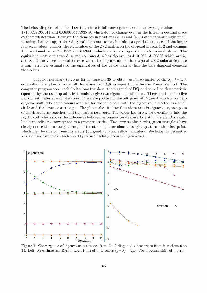
This section lists some facts in no particular order and §3 gives numerical examples. The n×n squarematrix E is assumed to have real elements, but is otherwise arbitrary unless stated. Some of theseproperties will also apply to complex elements, but they are not of interest to my type of vibrationmodelling, so I ignore them. The eigenvalues are λj and eigenvectors are pj , j = 1, n. v is a generaln-vector.
1. Eigenvalues and eigenvectors arise as solutions of the equation Ep = λp for all square matrices,invertible and non-invertible. Symmetric matrices have E = ET , where T denotes transpose.A symmetric matrix with real coefficients always has real eigenvalues and its eigenvectors aremutually orthogonal. A ‘positive definite’ matrix is a symmetric matrix such that for everyvector v, vTEv > 0 ; all its eigenvalues are real and positive. The form vTEv appears in thephysics of vibration as 1
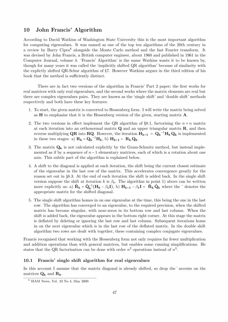
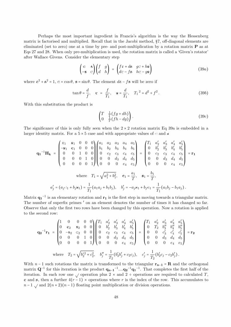
2vTMv for the kinetic energy and 1
2vTKv for potential strain energy.
M and K must be positive definite as energy cannot be negative.
2. The eigenvectors pj are only determined up to the ratio of their components. They are usuallynormalised by multiplying by a scale factor chosen to give one component the value 1, or tomake the modulus 1 so that each pj is a unit vector.
3. The trace of a square matrix (the algebraic sum of its diagonal elements) equals the algebraicsum of the eigenvalues. Hence in an n×n matrix if n− 1 eigenvalues have been found, the lastis given by subtracting from the trace.
4. Given an eigenvector p, the corresponding eigenvalue is readily found in one of two ways. i)Normalise the vector so that one component is 1 then multiply by E; that component will bereplaced by the eigenvalue. ii) Since Ep = λp, pTEp = λpTp. The dot product pTp = ∣p∣2so λ = pTEp/∣p∣2. This quantity is called the Rayleigh quotient after Lord Rayleigh who
4
introduced it in volume 1 of his book ‘The Theory of Sound’, his §90, page 113 et seq.. TheRayleigh quotient of a matrix achieves its least value when λ is the smallest absolute eigenvalue,corresponding for a vibrating system with the lowest frequency.
5. The eigenvectors are linearly independent, though not orthogonal unless the matrix is sym-metric. Two or more eigenvectors can share the same eigenvalue; the eigenvalue is then saidto be degenerate. For a non-degenerate matrix the eigenvectors form a complete basis set ofdimension n, meaning that they span the space of n dimensions. Then any other vector v inn dimensions can be written as a linear combination
v = c1p1 + c2p2 + ....cnpn. (2)
6. An important consequence of item 5 is that powers of E applied to an arbitrary vector vconverge to the eigenvector with the largest absolute eigenvalue. To see this, suppose that withsome relabelling λ1 > λ2 > ... > λn. Apply E repeatedly to Eq 2.
Ekv = c1λk1p1 + c2λk2p2 + ....cnλk1pn,
= c1λk1 (p1 +
c2λk2
c1λk1p2 + .... cnλ
kn
c1λk1) .
→ c1λk1p1 as k →∞ .
(3)
This is the basis of the Power Method for finding the eigenvalue of largest absolute valueand simultaneously the corresponding eigenvector. The method is described in §3. Clearlyconvergence depends on both the choice of initial vector (through c2/c1) and on the ratio ofabsolute eigenvalues ∣λ2∣/∣λ1∣.
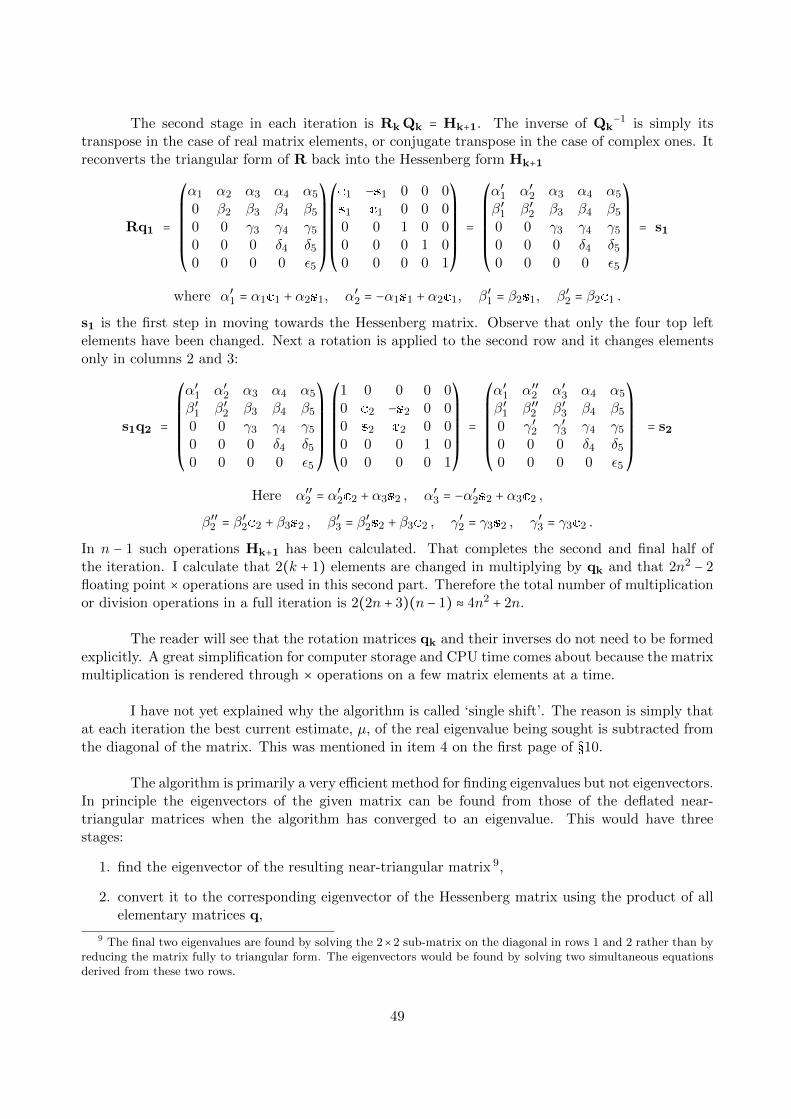
7. If elementary row operations of replacing a row by itself plus a multiple of another row areused to convert a matrix to triangular form, the signs of the diagonal elements (called the‘pivots’) give the signs of the eigenvalues, though not their values. The product of all thepivots happens to be the determinant of the original matrix. However, the elementary rowand column operations in general change the trace, the characteristic equation and hence theeigenvalues and eigenvectors.
8. If a constant β is subtracted from all the diagonal elements of E, the eigenvalues of E− βI areλj − β, 1 ≤ j ≤ n. This is called ‘shifting’. The proof is quite simple; (E − βI)p = λp − βIp =(λ − β)p. Shifting by a carefully chosen constant can be used to enhance the convergence ofthe Power Method by changing the ratio λ2/λ1.
9. The eigenvalues of the transpose ET are the same as those of E, but the eigenvectors aredifferent unless the matrix is symmetric. To prove this suppose that
Ep = λp and ETq = µq .
Using the order-reversing property of transposes,
qTE = µqT so qTEp = µqTp .
But qTEp is also obtained by multiplying Ep = λp on the left by qT , and it gives qTλp. Thisequals µqTp only if µ = λ.The relation qTE = λqT explains why qT is referred to as the ‘left eigenvector’ of E. p wouldthen be called the right eigenvector.
5
10. The eigenvectors of the inverse of a matrix E−1 are the same as the eigenvectors of E and itseigenvalues are the reciprocals 1/λj . The proof is: E−1Epj = E−1λj pj so pj = λjE−1 pj orE−1 pj = 1/λj pj . There is a close relation between the eigenvectors of the inverse E−1 and theeigenvectors of the transpose ET , described and used in §?? on ‘matrix deflation’ which is thename given to eliminating a selected eigenvalue-vector pair from a matrix.
11. Suppose we have three n×n matrices, E, F and G, where G is invertible. If they are related byE =G−1FG, then E and F are said to be ‘similar’ and linked by the similarity transformation(also called conjugate transformation) of pre-and post-multiplication by G. E and F have thesame determinant, characteristic equation, trace, and the same eigenvalues, though differenteigenvectors. To see this, observe that if Ep = λp, then FGp = λGp. So F also has eigenvalueλ, but eigenvector Gp. Similar matrices represent the same linear transformation of a spacefrom different sets of basis vectors.
12. A special case of the previous item is that a square matrix can be diagonalised – that is,represented by a diagonal matrix with the same eigenvalues and eigenvectors. The operationis effected by the matrix P whose columns are the column eigenvectors pj , i ≤ j ≤ n. Thus
D = P−1EP (4)
is diagonal, and its elements are its eigenvalues which are also the eigenvalues of E. Theeigenvectors are the orthogonal set (1,0,0, ...0), (0,1,0, ...0), .... ., (0,0,0, ....1). We have herea method for producing an infinite family of matrices with the same prescribed eigenvalues:start with a diagonal matrix built of the given eigenvalues and transform it with any choseninvertible matrix in a similarity transformation.
13. A triangular matrix (one with 0s below or above the main diagonal) also has its eigenvaluesarrayed down the diagonal. Only the diagonal elements contribute to the characteristic polyno-mial. If the eigenvalues are all real, the characteristic polynomial is a product of linear factors(λ1 − d11)(λ2 − d22) . . . (λN − dNN) where djj are the diagonal elements.
14. Several mathematicians have proved bounds on eigenvalues in terms of the value of the matrixelements. A simple test by Alfred Brauer, 1946, is based on the absolute values of the elements.Let aij be the elements, Ri = ∑j ∣aij ∣ be the sum of absolute values along the ith row and
Cj = ∑i ∣aij ∣ the sum down the jth column. Let R be the largest Ri and C the largest Cj . Thenfor all eigenvalues ∣λ∣ ≤min(R, C).
15. Other bounds were derived by Gershgorin (1931) by analogy with the diagonalised matrix Din item 11. He judged that if the off-diagonal elements are relatively small compared with thediagonal ones, the eigenvalues cannot be too far away from the values down the diagonal. Thisis quantified in Gershgorin’s two Circle Theorems. Let the n×n matrix have elements aij , andalong each row i add up the absolute values ∣aij ∣, i /= j of the off-diagonal elements. Call thissum ri. Next, in the complex plane mark a point on the real axis at the point correspondingto the diagonal element aii. Using this as centre, draw a circle with radius ri. Repeat thisfor all rows to give n such circles. These will overlap if some diagonal elements are close toeach other. Theorem I states that every eigenvalue lies within at least one of these circles.Theorem II states that if n1 circles overlap each other and another n2 overlap each other butare disjoint from the first set, then exactly n1 eigenvalues lie in the first set and n2 in thesecond. The circles allow for the possibility of the eigenvalues being complex, though I shallnot be concerned with such matrices. The theorem also holds if the sums of absolute valuesare taken down the columns instead of across the rows.
6
16. A third set of bounds on eigenvalues has been given by Wolkowicz and Styan (‘Bounds oneigenvalues using traces’ in Linear Algebra and its Applications, Vol 29, p 471-506, 1980).Suppose the n real eigenvalues of an n × n matrix are ordered λ1 ≥ λ2 ≥ ....λk ≥ .... ≥ λn. Byanalogy with statistics, Wolkowicz and Styan define a mean m and standard deviation s forthe trace of a matrix by
m = TrE
n= 1
n
n
∑j
λj , s2 = 1
n
2
[nTr(E2) − (TrE)2] = 1
nTr(E2) −m2 .
Then m − s√n − 1 ≤ λmin ≤ m − s√
n − 1,
m + s√n − 1
≤ λmax ≤ m + s√n − 1 ,
m − s√
k − 1
n − k + 1≤ λk ≤ m + s
√n − kk
.
As a special case, when n = 3
m − s√
2 ≤ λ3 ≤ m − s√2
≤ λ2 ≤ m + s√2
≤ λ1 ≤ m + s√
2 . (5)
17. There is a special class of matrix which arises is vibration analysis; a non-symmetric matrixmade by the product of two symmetric matrices. The eigenvectors of these have orthogonalityproperties which are crucial for vibration modal analysis2. This is seen in Eq 1 where M, M−1
and K are symmetric. If the eigenvectors of E =M−1K are pj , the orthogonality condition is
pTj Mpi = 0 if i /= j . (6)
If i = j, the product is non-zero and used to scale and normalise the components of theeigenvectors to make pTj Mpj = I, an operation called ‘mass normalisation’.
18. A matrix problem is said to be ‘ill-conditioned’ if numerical attempts to determine its solutions,such as finding the eigenvalues and eigenvectors, are over-sensitive to the precision of or errorsin the input numbers. The ‘condition number’ ≥ 1 is defined as the ratio of error in outputto error in the input and is given numerically as the product of the direct and inverse norms,∥E−1 ∥ . ∥E∥. Here ∥ ... ∥ denotes the Euclidean norm (also called the spectral or L2 norm)which is the square root of the sum of the squares of all the matrix elements. A large conditionnumber indicates troublesome sensitivity to input. Ill-conditioned matrices can arise in finite-element models where a few matrix elements are orders of magnitude different from the rest.In practice finding E−1 is a challenge so the condition number may have to be estimated fromintermediate numbers produced during a calculation.
19. The Cayley-Hamilton theorem: Each matrix satisfies its own characteristic equation. So ifthe matrix is E and its characteristic equation is anλ
n + an−1λn−1 + ..... + a1λ + a0 = 0, thenanE
n + an−1En−1 + .....+ a1E+ a0I = 0, the zero matrix. This provides a method for calculatinghigher powers of E, since En = −(an−1En−1 + .....+ a1E+ a0I)/an. Moreover, the inverse can befound as a polynomial in E since anE
n−1 + an−1En−2 + ..... + a1I = −a0E−1.
2 Proof of orthogonality is given in §2 of my article on modal vibration analysis on www.mathstudio.co.uk, entitled‘Periodic Forced Vibrations, Normal Modes and Damping, with Measurements on a ’Cello’.
7
20. The eigenvalues and eigenvectors of a positive definite matrix have a geometrical representationin terms of a ‘representation ellipsoid’. This is most readily envisaged with a diagonalised3-dimensional matrix, D. (Recall that all eigenvalues are real and positive and lie on thediagonal.) Consider the product vTDv with v = (x, y, z). This is the dot or inner product ofthe vectors v and Dv and evaluates to λ1x
2 + λ2y2 + λ3z2. The locus of points which satisfyλ1x
2 + λ2y2 + λ3z2 = 1 is an ellipsoid with semi-axes of lengths 1/√λ1, 1/
√λ2, 1/
√λ3 and
with principal axes along the x, y and z axes. If E is similar to D, it will also represent aquartic surface, but skewed and distorted. However three position vectors will be unchangedin direction by the transformation – these are the eigenvectors. The ellipsoid will be stretchedin these directions by amounts given by the respective eigenvalues. Note that each of thelengths 1/
√λj is a local maximum, minimum or stationary value with respect to small changes
in the vector direction. This has prompted an important concept that the eigenvalues andvectors in a more general sense maximise or minimise some function of the matrix. The areaof mathematical which investigates such problems is the ‘calculus of variations’.
3 Illustrative examples of matrix properties
Some numerical examples will help the reader appreciate the above interesting facts. I will take theeigenvalue with largest absolute value to be λ1, the next to be λ2.
3.1 A general 3 × 3 matrix
Our first example matrix is
E =⎛⎜⎝
−4 −2 31 3 4−1 1 5
⎞⎟⎠. (7)
Its trace is 4. To find bounds on the eigenvalues first apply Brauer’s criterion, §2.1, item 12. Thelargest absolute row sum is 9 and largest column sum is 12, so ∣λj ∣ ≤ 9. The matrix is not diagonallydominant, but let us see what Gershgorin theorems state as bounds of the eigenvalues. Applied tothe rows, the circle centres are at −4, 3 and 5 and the respective radii are 5, 5 and 2. These overlapand span from −9 to +8. Applied to the columns the circles span from −6 to 12 so together theeigenvalues must lie within (−6, 8), a modest narrowing of bounds from ±9. The circle for column1 spans (−6,2) and the other two overlap and together span (−2, 12). They only touch at −2 so itis likely that there is only one eigenvalue in (−6, −2) and two in (−2,8).
Solving for the eigenvalues in the classical analytic way, the characteristic equation is
and the zero matrix does result. Since we have here E2, we can evaluate the Wolkowicz-Styan boundsusing Eq 5 of item 14. m = 4/3 and s2 = 48/3−16/9 so s = 8
√2/3 = 3 ⋅77. The eigenvalues are bounded
−4 < λ < −113 < λ < 4 < λ < 62
3 .
8
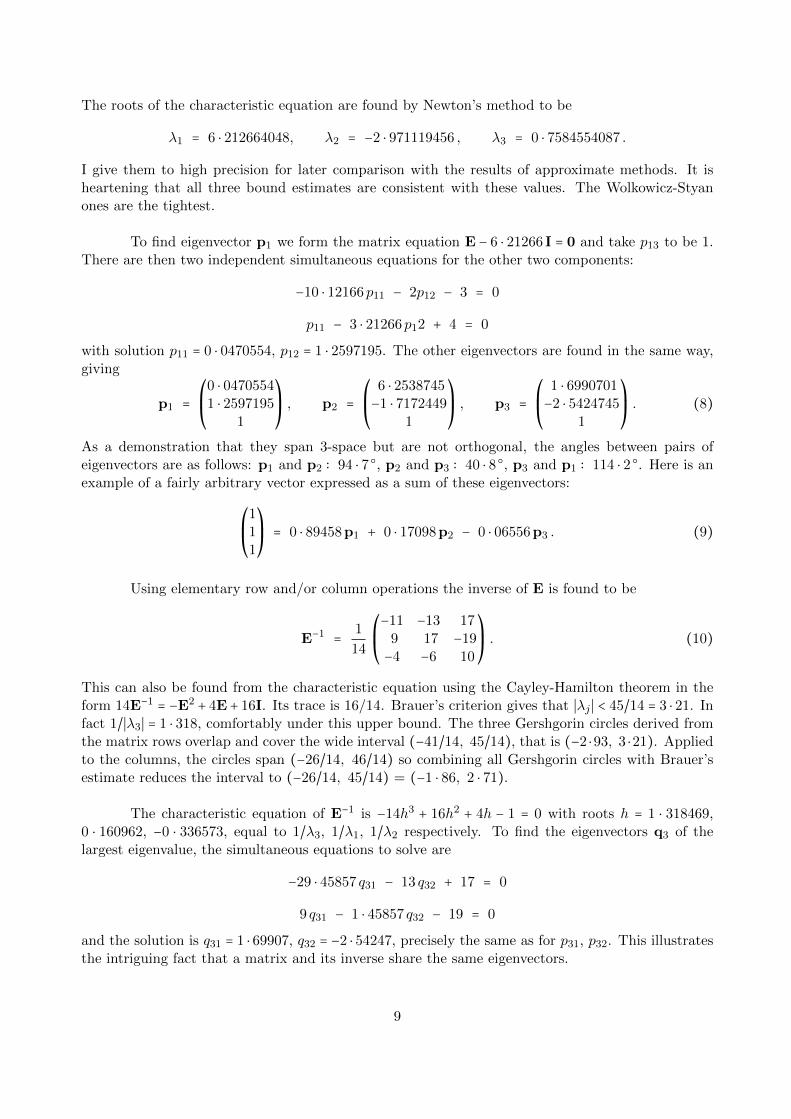
The roots of the characteristic equation are found by Newton’s method to be
I give them to high precision for later comparison with the results of approximate methods. It isheartening that all three bound estimates are consistent with these values. The Wolkowicz-Styanones are the tightest.
To find eigenvector p1 we form the matrix equation E − 6 ⋅ 21266 I = 0 and take p13 to be 1.There are then two independent simultaneous equations for the other two components:
−10 ⋅ 12166p11 − 2p12 − 3 = 0
p11 − 3 ⋅ 21266p12 + 4 = 0
with solution p11 = 0 ⋅ 0470554, p12 = 1 ⋅ 2597195. The other eigenvectors are found in the same way,giving
p1 =⎛⎜⎝
0 ⋅ 04705541 ⋅ 2597195
1
⎞⎟⎠, p2 =
⎛⎜⎝
6 ⋅ 2538745−1 ⋅ 7172449
1
⎞⎟⎠, p3 =
⎛⎜⎝
1 ⋅ 6990701−2 ⋅ 5424745
1
⎞⎟⎠. (8)
As a demonstration that they span 3-space but are not orthogonal, the angles between pairs ofeigenvectors are as follows: p1 and p2 ∶ 94 ⋅ 7 ○, p2 and p3 ∶ 40 ⋅ 8 ○, p3 and p1 ∶ 114 ⋅ 2 ○. Here is anexample of a fairly arbitrary vector expressed as a sum of these eigenvectors:
⎛⎜⎝
111
⎞⎟⎠
= 0 ⋅ 89458p1 + 0 ⋅ 17098p2 − 0 ⋅ 06556p3 . (9)
Using elementary row and/or column operations the inverse of E is found to be
E−1 = 1
14
⎛⎜⎝
−11 −13 179 17 −19−4 −6 10
⎞⎟⎠. (10)
This can also be found from the characteristic equation using the Cayley-Hamilton theorem in theform 14E−1 = −E2 + 4E+ 16I. Its trace is 16/14. Brauer’s criterion gives that ∣λj ∣ < 45/14 = 3 ⋅ 21. Infact 1/∣λ3∣ = 1 ⋅ 318, comfortably under this upper bound. The three Gershgorin circles derived fromthe matrix rows overlap and cover the wide interval (−41/14, 45/14), that is (−2 ⋅93, 3 ⋅21). Appliedto the columns, the circles span (−26/14, 46/14) so combining all Gershgorin circles with Brauer’sestimate reduces the interval to (−26/14, 45/14) = (−1 ⋅ 86, 2 ⋅ 71).
The characteristic equation of E−1 is −14h3 + 16h2 + 4h − 1 = 0 with roots h = 1 ⋅ 318469,0 ⋅ 160962, −0 ⋅ 336573, equal to 1/λ3, 1/λ1, 1/λ2 respectively. To find the eigenvectors q3 of thelargest eigenvalue, the simultaneous equations to solve are
−29 ⋅ 45857 q31 − 13 q32 + 17 = 0
9 q31 − 1 ⋅ 45857 q32 − 19 = 0
and the solution is q31 = 1 ⋅ 69907, q32 = −2 ⋅ 54247, precisely the same as for p31, p32. This illustratesthe intriguing fact that a matrix and its inverse share the same eigenvectors.
9
The matrix P and its inverse which will diagonalise E are
The transposed matrix ET has the same eigenvalues but these eigenvectors, which are pro-portional to the respective rows of P−1:
q1 =⎛⎜⎝
−0 ⋅ 0635640 ⋅ 350839
1
⎞⎟⎠, q2 =
⎛⎜⎝
−1 ⋅ 682395−0 ⋅ 730984
1
⎞⎟⎠, q3 =
⎛⎜⎝
−0 ⋅ 374042−0 ⋅ 779856
1
⎞⎟⎠.
Direct calculation shows that the dot (inner) product qTi pj = 0 if i /= j. Therefore qi and pj areorthogonal. A useful normalisation of the non-zero products sets the ∣pj ∣ = 1 and qTj pj = 1. I makeuse of this scheme in §5 on matrix deflation, but there introduce notation which has the eigenvectorsof E denoted x and normalised ∣xj ∣ = 1, and the eigenvectors of ET denoted y with yTj xj = 1. Thisleaves p and q meaning the same eigenvectors normalised such that the last vector component is 1.
3.2 A symmetric matrix
As an example, take
B =⎛⎜⎜⎜⎝
1 1 3 −11 2 5 13 5 −2 3−1 1 3 −2
⎞⎟⎟⎟⎠
and let us see what we can learn about its eigenvalues without solving the characteristic equation.The trace is −1. Brauer’s row-and-column sum test gives all ∣λ∣ < 13. In Wolkowicz and Styan’sstatistics criterion the trace of B2 is 105, so m = −1/4, s = 5 ⋅ 12. The intervals in which the foureigenvalues are predicted to lie overlap:
Using elementary row addition and multiplication operations I have transformed B to arow-equivalent triangular matrix
T =⎛⎜⎜⎜⎝
1 1 3 −10 1 2 20 0 −15 20 0 0 −101
⎞⎟⎟⎟⎠.
Note that no target row is multiplied by a negative number in these row operations as that wouldchange the sign of the pivot. The pivots are the diagonal elements and their signs show that two
10
eigenvalues are positive, two negative. We can immediately revise the bounds from Wolkowicz andStyan to
By subtracting a constant β from the diagonal elements, the value dividing positive from negativeeigenvalues is moved by β. This allows us to test various ranges to see if an eigenvalue lies within agiven range. For instance, take β = 4. The shifted matrix and its row-equivalent triangular matrixare
⎛⎜⎜⎜⎝
−3 1 3 −11 −2 5 13 5 −6 3−1 1 3 −6
⎞⎟⎟⎟⎠→
⎛⎜⎜⎜⎝
−3 1 3 −10 −30 108 120 0 93 220 0 0 −599
⎞⎟⎟⎟⎠.
This has three negative pivots so only one of λj − 4, j = 1, 4 is positive: that is, only one eigenvalueis > 4. Since there are two < 0, there must be exactly one in the interval (0, 4). Similarly shiftingby adding 4 gives
⎛⎜⎜⎜⎝
5 1 3 −11 6 5 13 5 2 3−1 1 3 2
⎞⎟⎟⎟⎠→
⎛⎜⎜⎜⎝
5 1 3 −10 29 22 60 0 −7 60 0 0 27
⎞⎟⎟⎟⎠
which has only one negative pivot. So one of λj + 4 is < 0, or one < −4. Taking all this evidencetogether we know that the eigenvalues are ordered
This case study illustrates how we can gain a rough idea of the positions of the eigenvalues on thereal number line. This may guide the choice of algorithms and indeed the whole strategy for solvingthe problem. However, we still have no idea as to the eigenvectors.
Solving in the classic way, the characteristic equation is λ4 + λ3 − 52λ2 − 47λ + 101 = 0 withsolutions
where they are indexed in order of absolute value. These values lie within the predicted intervals.The corresponding eigenvectors are
p1 =⎛⎜⎜⎜⎝
0 ⋅ 67053590 ⋅ 7691055−1 ⋅ 7347554
1
⎞⎟⎟⎟⎠, p2 =
⎛⎜⎜⎜⎝
1 ⋅ 59495803 ⋅ 02932222 ⋅ 5360030
1
⎞⎟⎟⎟⎠, p3 =
⎛⎜⎜⎜⎝
0 ⋅ 2432323−0 ⋅ 74350090 ⋅ 3408350
1
⎞⎟⎟⎟⎠, p4 =
⎛⎜⎜⎜⎝
−2 ⋅ 08499730 ⋅ 69996240 ⋅ 0808640
1
⎞⎟⎟⎟⎠.
The pair-wise dot products of these are all zero to within machine accuracy, proving that these area mutually orthogonal set. This is always the case with symmetric matrices.
3.3 Products of symmetric matrices
Matrices of the form AB, where A and B are symmetric, occur in finite element calculations asM−1K where M and K represent the mass and stiffness distributions of the structure. Here is asimple contrived example to illustrate that the eigenvectors are orthogonal with respect to weight
11
functions A−1 and B. Two arbitrary symmetric matrices will in general give complex eigenvalues,so I have chose A and B so that E =AB has only real ones. Let
A =⎛⎜⎜⎜⎝
1 1 4 01 2 5 04 5 −2 10 0 1 6
⎞⎟⎟⎟⎠, B =
⎛⎜⎜⎜⎝
1 1 3 −11 2 5 13 5 −2 3−1 1 3 −2
⎞⎟⎟⎟⎠.
We also need to know that
A−1 = 1
115
⎛⎜⎜⎜⎝
176 −133 18 −3−133 109 6 −118 6 −6 1−3 −1 1 19
⎞⎟⎟⎟⎠, E =AB =
⎛⎜⎜⎜⎝
14 23 0 1218 30 3 162 5 44 −7−3 11 16 −9
⎞⎟⎟⎟⎠.
The characteristic equation for E is λ4 − 79λ3 + 1107λ2 + 17062λ − 11615 = 0 with roots 50 ⋅ 43142,37 ⋅ 34133, −9 ⋅ 42702, 0 ⋅ 65427 and respective eigenvectors pj
⎛⎜⎜⎜⎝
2 ⋅ 278003 ⋅ 086562 ⋅ 01958
1
⎞⎟⎟⎟⎠,
⎛⎜⎜⎜⎝
−3 ⋅ 2814−3 ⋅ 851844 ⋅ 92921
1
⎞⎟⎟⎟⎠,
⎛⎜⎜⎜⎝
−0 ⋅ 183353−0 ⋅ 3349820 ⋅ 169233
1
⎞⎟⎟⎟⎠,
⎛⎜⎜⎜⎝
−1 ⋅ 309000 ⋅ 2378100 ⋅ 194459
1
⎞⎟⎟⎟⎠.
Incidentally, there is no simple relationship between the eigenvalues and eigenvectors of A, B andE. The point to be demonstrated is that pi
TA−1pj = 0 and piiBPj = 0 unless i = j. I have confirmed
this for the above matrices, obtaining products of typically 10−14, which is essentially 0 to machineaccuracy.
Here is a proof of this intriguing fact. The eigenvalue equation is A−1Bpi = λipi. Use theproperty of transposes that CDT =DTCT to show that
pTi BT (A−1)T = λipTi .
Since A, and hence A−1, and B are symmetric,
pTi BA−1 = λipTi .
Now multiply on the right by Apj to get
pTi Bpj = λipTi Apj . (11a)
Swap the labels and take the transform
(pTj Bpi)T = λj(pTj Api)T .
pTi Bpj = λjpTi Apj . (11b)
The left sides of Eq 6a and b are the same and their right sides differ only through the subscripts onλ. But the eigenvalues λi and λj are not equal, so their multiplying factors must be zero.
12
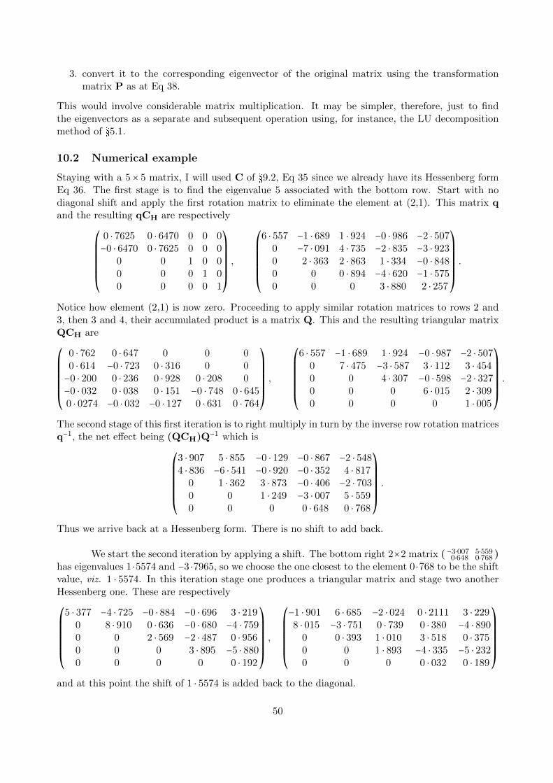
3.4 A degenerate matrix
Here is an example of a matrix with three equal eigenvalues: λ1 = λ2 = λ3 = 3, λ4 = 1.
A =⎛⎜⎜⎜⎝
3 0 0 0−2 2 0 10 0 3 02 1 0 2
⎞⎟⎟⎟⎠.
The trace is 10, the determinant 27 and the characteristic equation is (λ−3)3 (λ−1) = 0. Substitutingλ = 1 into (A−λI)p gives the eigenvector p4 = (0,−1,0,1). Substituting λ = 3 gives only one relationamongst the vector components 2pj1 + pj2 − pj4 = 0, j = 1,3. Geometrically, this is the equation of aplane and so must be spanned by two independent vectors. There is wide scope to choose two basisvectors for this space, but (0,1,1,1) and (14 ,
12 ,0,1) will serve – they both have the last component
equal to 1. Alternatively the Gram-Schmidt procedure can be used to produce two orthonormal basevectors
b1 =⎛⎜⎜⎜⎝
0 ⋅ 574285−0 ⋅ 6075170 ⋅ 0915490 ⋅ 541053
⎞⎟⎟⎟⎠, b2 =
⎛⎜⎜⎜⎝
−0 ⋅ 0345080 ⋅ 3600200 ⋅ 8857260 ⋅ 291005
⎞⎟⎟⎟⎠.
We see that each of the three equal eigenvalues does not have associated with it a unique eigenvector,but instead the three share a space, here equivalent to a plane. Degenerate matrices are likely to arisein engineering and physics where the structure being described has rotational or mirror symmetry.
4 The direct power method
The Power Method was known in Victorian times as an iterative procedure converging on the eigen-value with the largest absolute value and simultaneously upon its eigenvector. Indeed, the algorithmfocuses on the eigenvector and produces the eigenvalue as a by-product. It exists to two forms,direct and inverse, the latter being described in the next section, §4. As above, the largest absoluteeigenvalue is called λ1, the second λ2, etc.
4.1 Matrix multiplication in the basic power method
The basic power method operates as follows. Using the example in §3.1, apply E of Eq 7 repeatedlyto the vector v = (1,1,1). This is a fairly arbitrary starting place, though the linear expansion interms of the eigenvectors at Eq 8 does show that p1 makes the largest contribution. Some values are
E3v =⎛⎜⎝
−18278210
⎞⎟⎠, E4v =
⎛⎜⎝
14616561346
⎞⎟⎠, E5v =
⎛⎜⎝
142104988240
⎞⎟⎠, E6v =
⎛⎜⎝
31566459651556
⎞⎟⎠.
This looks opaque until the matrices are normalised by scaling so that, say, the bottom componentis 1. Some values are
E3v →⎛⎜⎝
−0 ⋅ 085711 ⋅ 32381
1
⎞⎟⎠, E4v →
⎛⎜⎝
0 ⋅ 108471 ⋅ 23031
1
⎞⎟⎠, E5v →
⎛⎜⎝
0 ⋅ 017231 ⋅ 27403
1
⎞⎟⎠, E6v →
⎛⎜⎝
0 ⋅ 061211 ⋅ 25293
1
⎞⎟⎠.
By iteration 20 the agreement with p1 is correct to 6 decimal places. If a further multiplication ismake on the normalised vector we get
v20 =⎛⎜⎝
0 ⋅ 04705441 ⋅ 2597199
1
⎞⎟⎠, Ev20 ≈ λ1v20 =
⎛⎜⎝
0 ⋅ 29233807 ⋅ 82621356 ⋅ 2126633
⎞⎟⎠.
13
The bottom component is the largest eigenvalue, λ1, correct almost to 6 decimal places. In practicethe normalisation would be performed at each iteration and the cycle stopped when the differencebetween successive iterations is less than, say, 10−8.
The subtleties are in encouraging the method to converge fairly rapidly whatever the valuesof the eigenvectors. I now give some algebraic analysis of convergence. Using superscripts to indexthe iterations, suppose that the starting guess is the vector in Eq 2,
v(0) = c1p1 + c2p2 + .... cnpn Copy of (2)
where the last component of each pj is 1 and the eigenvalues are ordered ∣λ1∣ > ∣λ2∣ > .... > ∣λn∣.Multiply by E and renormalise:
Even though c1 may be much smaller that c2 (a possibility examined below), it is clear that (λ1/λ2)m
will grow indefinitely with m while (λ2/λ1)m will shrink. Therefore c(m)1 → 1 and c
(m)j → 0, j ≥ 2,
and v(m) → p1. Subject to control of rounding errors, the iterations will almost certainly convergeon the eigenvector for the largest eigenvalue, provided ∣λ2∣ /= λ1.
What starting vector would give the worse convergence? Theoretically if c1 = 0, convergenceto p1 should be impossible. Because the eigenvectors are not orthogonal, it is not sufficient to inventa starting vector v(0) which is just a linear combination of p2 and p2; it is also necessary for it beto normal to p1. The vector with these properties is (9 ⋅ 4104456, −1 ⋅ 1453442, 1). After only twomultiplications by E it is clear that the pull of λ1 has been suppressed and that the v(j) are tendingtowards the second largest eigenvector, p2. Closest approach to p2 is attained at 12 iterations wherethe error in λ2 is about 3×10⁻⁷. Perhaps surprisingly, with more iterations it diverges from p2 in thedirection of p1. After 50 iterations the method has λ1 and its eigenvector correct to 3 decimal places.The power method, therefore, has an inevitability pull towards the eigenvector whose eigenvalue hasthe largest magnitude.
Even with a favourable choice of starting vector the rate of convergence will depend stronglyon λ1/λ2 and to a lesser extent on c1/c2. To emphasise these, let us evaluate the difference δm+1 =
14
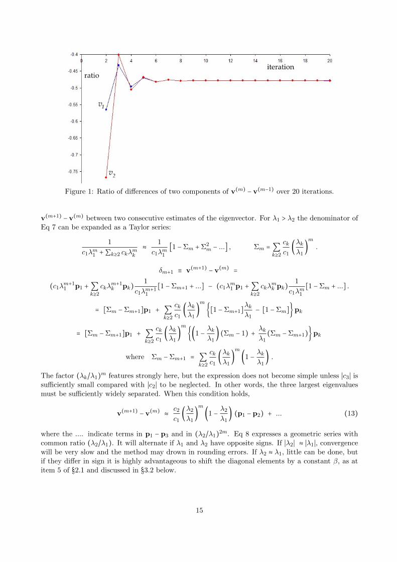
Figure 1: Ratio of differences of two components of v(m) − v(m−1) over 20 iterations.
v(m+1) −v(m) between two consecutive estimates of the eigenvector. For λ1 > λ2 the denominator ofEq 7 can be expanded as a Taylor series:
1
c1λm1 +∑k≥2 ckλmk≈ 1
c1λm1[1 −Σm +Σ2
m − ...] , Σm = ∑k≥2
ckc1
(λkλ1
)m
.
δm+1 ≡ v(m+1) − v(m) =
(c1λm+11 p1 +∑k≥2
ckλm+1k pk)
1
c1λm+11
[1 −Σm+1 + ...] − (c1λm1 p1 +∑k≥2
ckλmk pk)
1
c1λm1[1 −Σm + ...] .
= [Σm −Σm+1]p1 + ∑k≥2
ckc1
(λkλ1
)m
{[1 −Σm+1]λkλ1
− [1 −Σm]}pk
= [Σm −Σm+1]p1 + ∑k≥2
ckc1
(λkλ1
)m
{(1 − λkλ1
) (Σm − 1) + λkλ1
(Σm −Σm+1)}pk
where Σm −Σm+1 = ∑k≥2
ckc1
(λkλ1
)m
(1 − λkλ1
) .
The factor (λk/λ1)m features strongly here, but the expression does not become simple unless ∣c3∣ issufficiently small compared with ∣c2∣ to be neglected. In other words, the three largest eigenvaluesmust be sufficiently widely separated. When this condition holds,
v(m+1) − v(m) ≈ c2c1
(λ2λ1
)m
(1 − λ2λ1
) (p1 − p2) + ... (13)
where the .... indicate terms in p1 − p3 and in (λ2/λ1)2m. Eq 8 expresses a geometric series withcommon ratio (λ2/λ1). It will alternate if λ1 and λ2 have opposite signs. If ∣λ2∣ ≈ ∣λ1∣, convergencewill be very slow and the method may drown in rounding errors. If λ2 ≈ λ1, little can be done, butif they differ in sign it is highly advantageous to shift the diagonal elements by a constant β, as atitem 5 of §2.1 and discussed in §3.2 below.
15
As numerical evidence for a geometric series, Figure 1 plots in blue the ratio
v(m)1 − v(m−1)1
v(m−1)1 − v(m−2)1
of the first component v(m)1 of v(m) obtained with the matrix E of §3.1. The red points are ratios
for the second component v(m)2 . (The third component is normalised to 1 for all v(m) .) Even at
iteration 5 the ratios for the two components are close, being respectively −0 ⋅ 470 and −0 ⋅ 468. Atiteration 10 they agree on −0 ⋅ 478430 to 6 decimal places. At this stage the λ1 eigenvalue has beendetermined as 6 ⋅215 so the common ratio tells us that λ2 is close to −2 ⋅973. Moreover, if all we wereinterested in were the eigenvalues and not the other two eigenvectors for this 3 × 3 matrix E, λ3 isTrace−λ1 − λ2 = 0 ⋅ 758. All three eigenvalues have been found from one short sequence of iterationson one starting vector.
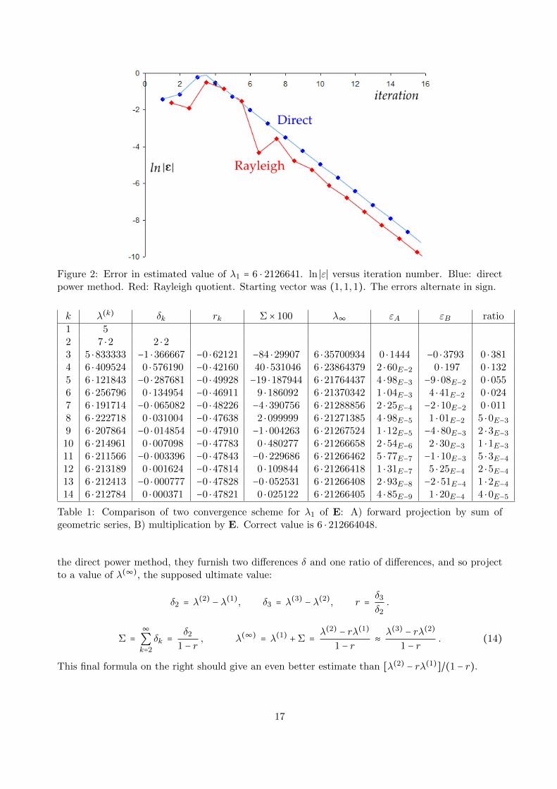
4.1.1 Rayleigh quotients
I should point out that there is an alternative way of calculating the iterated eigenvalue using theRayleigh quotient, introduced at item 3 in §2. Writing µk for the estimated eigenvalue at the kth
iteration (so as not to confuse it with the λ obtained by direct multiplication)
Ev(k) = µkv(k) so v(k)TEv(k) = µkv(k)Tv(k) and µk =v(k)TEv(k)
v(k)Tv(k).
The expression on the right is the Rayleigh quotient. It involves extra calculation beyond determiningEv(k) and so is a half-way-house between iterations k and k + 1 of the direct power method. Toillustrate this Figure 2 plots the natural logarithm of the absolute error in the estimated eigenvalueof our example matrix E of Eq 7. The number of the iteration forms the horizontal axis and I haveplotted the points for the direct power method at integer values and the Rayleigh quotient valuesat the next 1
2 . For this case Rayleigh quotient is slightly more accurate than the next direct powerestimate, though it converges at the same rate. It is a matter of judgement whether it is worth theextra effort in calculation compared with making another couple of multiplications by E.
4.2 Predicted values using summed geometric series
There is considerable scope to improve the estimation of the eigenvector components and leadingeigenvalue using the fact that the differences between successive iterations form geometric series. Ipresent here a summary and refer the reader to Appendix 1 for supporting analysis. The essentialconcept is that if the first term C and common ratio r of a geometric series can be identified, thenthe sum to infinity, S, is given by the formula we learned at school
S = C1 − r
, ∣r∣ < 1 .
This allows the value currently estimated by the basic power method – by multiplication by E – tobe projected as if through an infinity of further iterations to the true value. Indeed if the differencesδm did form exactly a single geometric series, the precise values of p and λ would be known after onlythree consecutive iterates. I have not seen this aspect of the Power Method described in textbooksor the literature, but it seems quite obvious so I suppose it to be well known. The analysis here ismy own.
Consider the first order approximation where a single geometric series is used to project avalue for the eigenvalue. When three consecutive evaluations, λ(1), λ(2), λ(3), have been made by
16
Figure 2: Error in estimated value of λ1 = 6 ⋅ 2126641. ln ∣ε∣ versus iteration number. Blue: directpower method. Red: Rayleigh quotient. Starting vector was (1,1,1). The errors alternate in sign.
Table 1: Comparison of two convergence scheme for λ1 of E: A) forward projection by sum ofgeometric series, B) multiplication by E. Correct value is 6 ⋅ 212664048.
the direct power method, they furnish two differences δ and one ratio of differences, and so projectto a value of λ(∞), the supposed ultimate value:
δ2 = λ(2) − λ(1), δ3 = λ(3) − λ(2), r = δ3δ2.
Σ =∞∑k=2
δk = δ21 − r
, λ(∞) = λ(1) +Σ = λ(2) − rλ(1)
1 − r≈ λ(3) − rλ(2)
1 − r. (14)
This final formula on the right should give an even better estimate than [λ(2) − rλ(1)]/(1 − r).
17
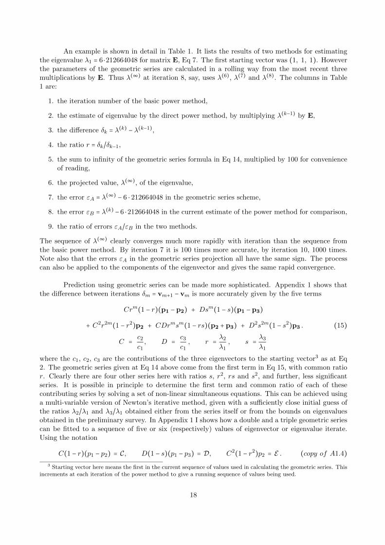
An example is shown in detail in Table 1. It lists the results of two methods for estimatingthe eigenvalue λ1 = 6 ⋅212664048 for matrix E, Eq 7. The first starting vector was (1, 1, 1). Howeverthe parameters of the geometric series are calculated in a rolling way from the most recent threemultiplications by E. Thus λ(∞) at iteration 8, say, uses λ(6), λ(7) and λ(8). The columns in Table1 are:
1. the iteration number of the basic power method,
2. the estimate of eigenvalue by the direct power method, by multiplying λ(k−1) by E,
3. the difference δk = λ(k) − λ(k−1),
4. the ratio r = δk/δk−1,
5. the sum to infinity of the geometric series formula in Eq 14, multiplied by 100 for convenienceof reading,
6. the projected value, λ(∞), of the eigenvalue,
7. the error εA = λ(∞) − 6 ⋅ 212664048 in the geometric series scheme,
8. the error εB = λ(k) −6 ⋅212664048 in the current estimate of the power method for comparison,
9. the ratio of errors εA/εB in the two methods.
The sequence of λ(∞) clearly converges much more rapidly with iteration than the sequence fromthe basic power method. By iteration 7 it is 100 times more accurate, by iteration 10, 1000 times.Note also that the errors εA in the geometric series projection all have the same sign. The processcan also be applied to the components of the eigenvector and gives the same rapid convergence.
Prediction using geometric series can be made more sophisticated. Appendix 1 shows thatthe difference between iterations δm = vm+1 − vm is more accurately given by the five terms
where the c1, c2, c3 are the contributions of the three eigenvectors to the starting vector3 as at Eq2. The geometric series given at Eq 14 above come from the first term in Eq 15, with common ratior. Clearly there are four other series here with ratios s, r2, rs and s2, and further, less significantseries. It is possible in principle to determine the first term and common ratio of each of thesecontributing series by solving a set of non-linear simultaneous equations. This can be achieved usinga multi-variable version of Newton’s iterative method, given with a sufficiently close initial guess ofthe ratios λ2/λ1 and λ3/λ1 obtained either from the series itself or from the bounds on eigenvaluesobtained in the preliminary survey. In Appendix 1 I shows how a double and a triple geometric seriescan be fitted to a sequence of five or six (respectively) values of eigenvector or eigenvalue iterate.Using the notation
C(1 − r)(p1 − p2) = C, D(1 − s)(p1 − p3) = D, C2(1 − r2)p2 = E . (copy of A1.4)3 Starting vector here means the first in the current sequence of values used in calculating the geometric series. This
increments at each iteration of the power method to give a running sequence of values being used.
18
iteration power single double triplemethod series series series
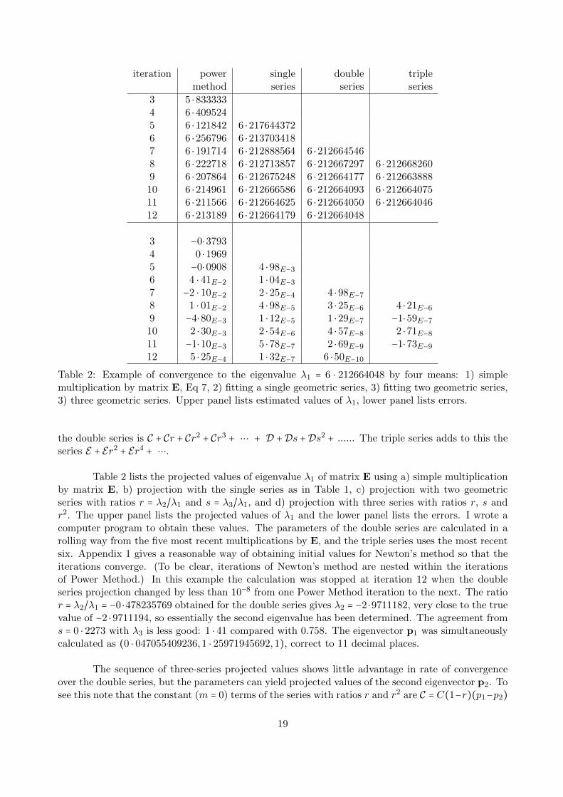
Table 2: Example of convergence to the eigenvalue λ1 = 6 ⋅ 212664048 by four means: 1) simplemultiplication by matrix E, Eq 7, 2) fitting a single geometric series, 3) fitting two geometric series,3) three geometric series. Upper panel lists estimated values of λ1, lower panel lists errors.
the double series is C + Cr + Cr2 + Cr3 + ⋯ + D +Ds +Ds2 + ...... The triple series adds to this theseries E + Er2 + Er4 + ⋯.
Table 2 lists the projected values of eigenvalue λ1 of matrix E using a) simple multiplicationby matrix E, b) projection with the single series as in Table 1, c) projection with two geometricseries with ratios r = λ2/λ1 and s = λ3/λ1, and d) projection with three series with ratios r, s andr2. The upper panel lists the projected values of λ1 and the lower panel lists the errors. I wrote acomputer program to obtain these values. The parameters of the double series are calculated in arolling way from the five most recent multiplications by E, and the triple series uses the most recentsix. Appendix 1 gives a reasonable way of obtaining initial values for Newton’s method so that theiterations converge. (To be clear, iterations of Newton’s method are nested within the iterationsof Power Method.) In this example the calculation was stopped at iteration 12 when the doubleseries projection changed by less than 10−8 from one Power Method iteration to the next. The ratior = λ2/λ1 = −0 ⋅478235769 obtained for the double series gives λ2 = −2 ⋅9711182, very close to the truevalue of −2 ⋅ 9711194, so essentially the second eigenvalue has been determined. The agreement froms = 0 ⋅ 2273 with λ3 is less good: 1 ⋅ 41 compared with 0.758. The eigenvector p1 was simultaneouslycalculated as (0 ⋅ 047055409236,1 ⋅ 25971945692,1), correct to 11 decimal places.
The sequence of three-series projected values shows little advantage in rate of convergenceover the double series, but the parameters can yield projected values of the second eigenvector p2. Tosee this note that the constant (m = 0) terms of the series with ratios r and r2 are C = C(1−r)(p1−p2)
19
and EC2(1 − r2)p2 respectively. Given numerical values for these and of the component p1 justcalculated, we have two simultaneous quadratic equations in C and p2. For example, in the calculationwhich gave Table 2 at iteration 11 the parameters for the first component of the dominant eigenvectorwere
C = −0 ⋅ 02098 , E = 0 ⋅ 00002338 , r = −0.478236 .
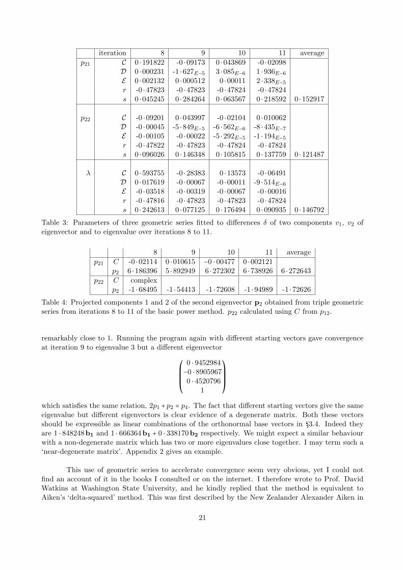
The solution is C = c2/c1 = 0 ⋅ 002121, p2 = 6 ⋅ 739. If you refer back the exact eigenvector as Eq 8,the correct value is about 6 ⋅ 254. The parameters fitted to the triple geometric series for iterations8 to 11 are listed in Table 3. p21 refers to the first component of the eigenvector p2, and p22 to thesecond, the third being normalised to 1. A few things to note in this table are
� the values of r = λ2/λ1 are very close and consistent and agree to about 6 decimal places withthe r values in the double series.
� the values of s = λ3/λ1 are more scattered. Averages are shown in the right panel. Theseaverages give λ3 = 0 ⋅ 87, to compare with the true value of 0 ⋅ 758. Although the double serieshas a much more consistent value of s at 0 ⋅ 227, the projected λ3 = 1 ⋅ 41 is about twice thecorrect value.
The above solution of two simultaneous equations can be done for each iteration, so I list thesolutions, C = c2/c1 and p21, in Table 4. The first column states the component of p2 and the secondnames the variables in the simultaneous equations. With the first eigenvector component solutionsat all four iterations are consistent. Their average is 6 ⋅ 2726 which compares well with the correctvalue of 6 ⋅ 264 (refer to Eq 8, §2.2.1). It is disappointing to find that the solutions for the secondvector component are complex. I have no explanation for this. However in any iteration the value ofC obtained for component p21 should also hold for p21. Using this C with the values of C in the p22panel of Table 3 give the values in the bottom row of Table 4. These average at −1 ⋅ 726, comparedwith the true value of −1 ⋅ 717.
To summarise, by fitting a double and a triple geometric series to four or then five consecutivevalues of the differences δ maximum information has been wrung from the power series iterations.The basic power method would have resulted in an estimate of p1 and λ1 accurate after 12 iterationsto 5× 10⁻⁴. After the same 12 iterations the double series has found p1 and λ1 to 6× 10⁻¹⁰, and alsoλ2 to 6 decimal places. The triple geometric series has added a useful approximation to the secondeigenvector p2 as (6 ⋅ 273, −1 ⋅ 726, 1). This is an excellent starting point for a power method searchfor precise p2 = (6 ⋅ 254, −1 ⋅ 7171, 1). The weakness in fitting the double and triple geometric seriesis in obtaining convergence of Newton’s method.
It is interesting to see what the power method with geometric series project makes of thedegenerate matrix of §3.4. I ran the computer program I had written to implement the direct powermethod, giving three arbitrary starting vectors from which the program chooses the best after threeiterations. At iteration 9 it stopped, having converged through the triple-series projection to λ1 = 3with error (that is, change from the last iteration) less that 2 ⋅ 5 × 10−9 and eigenvector
⎛⎜⎜⎜⎝
1 ⋅ 0614213−1 ⋅ 12284260 ⋅ 1692047
1
⎞⎟⎟⎟⎠.
This does satisfy the relation amongst the vector component given in §3.4 that 2p1 + p2 = p4 for anyp3. The ratio r in the geometric series pointed to the second largest eigenvalue being 0 ⋅ 999985,
Table 3: Parameters of three geometric series fitted to differences δ of two components v1, v2 ofeigenvector and to eigenvalue over iterations 8 to 11.
Table 4: Projected components 1 and 2 of the second eigenvector p2 obtained from triple geometricseries from iterations 8 to 11 of the basic power method. p22 calculated using C from p12.
remarkably close to 1. Running the program again with different starting vectors gave convergenceat iteration 9 to eigenvalue 3 but a different eigenvector
⎛⎜⎜⎜⎝
0 ⋅ 9452984−0 ⋅ 89059670 ⋅ 4520796
1
⎞⎟⎟⎟⎠
which satisfies the same relation, 2p1 +p2 = p4. The fact that different starting vectors give the sameeigenvalue but different eigenvectors is clear evidence of a degenerate matrix. Both these vectorsshould be expressible as linear combinations of the orthonormal base vectors in §3.4. Indeed theyare 1 ⋅ 848248b1 and 1 ⋅ 666364b1 + 0 ⋅ 338170b2 respectively. We might expect a similar behaviourwith a non-degenerate matrix which has two or more eigenvalues close together. I may term such a‘near-degenerate matrix’. Appendix 2 gives an example.
This use of geometric series to accelerate convergence seem very obvious, yet I could notfind an account of it in the books I consulted or on the internet. I therefore wrote to Prof. DavidWatkins at Washington State University, and he kindly replied that the method is equivalent toAiken’s ‘delta-squared’ method. This was first described by the New Zealander Alexander Aiken in
21
1927 as a general method for accelerating the convergence of any series that is geometric or almostgeometric. David Watkins explains
The extrapolation technique is equivalent to Aitken acceleration (Aitken’s delta-squaredprocess), found in Wilkinson’s book (page 578) and covered in many numerical analysistexts. It is not usually presented in terms of geometric series, but it is nevertheless thesame. I didn’t make use of Aitken acceleration in either of my books.
Aitken acceleration is useful whenever a sequence converges linearly, or geometricallyas you call it. The QR algorithm with standard shifting strategies normally convergesquadratically, so Aitken is not of use there. I think that is the reason Aitken has notbecome an important tool in the world of eigenvalue computations. It is only good foraccelerating linearly convergent processes, and it is not competitive against quadraticallyconvergent processes.
4.3 Shifting to improve convergence
Shifting the diagonal elements of the matrix is a way to manipulate the ratio of largest to next largesteigenvalues and so promote convergence. As shown at point 7 in §2.1, the offset β changes the ratioof eigenvalues to
λ1 + βλ2 + β
(16)
and this is largest when β = −λ2. Using our example 3 × 3 matrix E, suppose that with some happyguess of starting vector it is becoming clear after a few iterations that λ1 is near 6 ⋅ 2. Now λ2 isunknown, but we do know that the average value of λ2 and λ3 is (Trace−λ1)/2. The convergencerate towards λ1 can be increased with β = (4− 6 ⋅ 2)/2 = −1 ⋅ 1, the mean of the other eigenvalues. Toconfirm this numerically note the following alternative calculations. Taking (1, 1, 1 ) as the startingvector v(0) and no shift of diagonal elements, the first five estimates of largest eigenvalue are 5, 7 ⋅ 2,5 ⋅ 83, 6 ⋅ 4 and 6 ⋅ 12. A measure of change between consecutive estimates v(m) and v(m+1) next
is required, so I use δ defined as√
(∑[v(m+1)j − v(m)j ]2) where v(m)j is the jth component of vector
v(m). δ is the length of the vector joining the points defined by v(m) and v(m+1) when regarded asposition vectors. If the iterations continue with no shift, δ reduces to 7 ⋅ 6 × 10−7 at 21 iterations ofthe direct power method. If instead E is replaced by E − 1 ⋅ 1 I after the first five iterations, δ hasreduced to the same level after 9 further iterations, making 14 in all. This is not a great saving incalculational effort in this case, but still cuts it to 2/3. The eigenvalue arrived at is 7 ⋅ 312665 whichneeds adjusting downwards by 1 ⋅ 1. The other two eigenvalues, could they be found, are −1 ⋅ 87 and+1 ⋅ 86, straddling zero evenly, the best that could be achieved by choice of β.
Having found λ1 a second eigenvalue-vector pair can be found by shifting by β = λ1 tomake λ1 play no role in the iteration sequence. If λ1 is positive and λ2 is negative, as here, theshifted sequence will converge to λ2. If λ2 is also positive, shifting by λ1 will give convergence onλ3. Multiplying (1, 1, 1 ) a few times by E − 6 ⋅ 2 I, the first four eigenvalue estimates are −1 ⋅ 2,−10 ⋅ 4, −9 ⋅ 75, −9 ⋅ 5 and, if allowed to continue with β = 6 ⋅ 2, δ falls to 9 × 10⁻⁷ by iteration 27.It is possible to optimise β as above based on the estimate λ2 ≈ −9 ⋅ 2 + 6 ⋅ 2 = −3 ⋅ 0. With β setto (Trace−(−3 ⋅ 0))/2 = 3 ⋅ 5 after the first four iterations, in a further 15 iterations (19 in all) δ hasreduced to 7 × 10⁻⁷, another modest but worthwhile improvement in convergence rate. The othertwo eigenvalues have been shifted to 2 ⋅ 71 and −2 ⋅ 74 giving the smallest absolute value of the nextlargest eigenvalue.
22
This suggests a two stage approach to finding an eigenvalue λ. First a few iterations onthe starting vector are used to find a rough value, then a shift of matrix diagonal is introduced toenhance the rate of convergence. Since a poor choice of starting vector will give poor convergence atthe start of the process, it is probably worth trying two or three vectors and picking the one whichhas the smallest change δ at each step, since small changes in the iterates signal closeness of thetrue value. Three starting choices might be (1, 1, 1 ), (1, −2, 1 ) and (−1, 0, 1 ), which are mutuallyorthogonal. Further increase is the rate of convergence will probably be possible using the summedgeometric series described in §3.2. We see that in the direct power method there is considerablescope for rapidly finding at least some of the eigenvector-value pairs.
In Appendix 1, §9, I give details of an attempt to find the eigen pairs of a challenging 6 × 6matrix which has some eigenvalues close together.
5 Inverse power method with LU decomposition
Can the Power Method be adapted further to find the third and further eigenvalue-eigenvector pairs?The Inverse Power Method is a scheme which applies the iteration process not to E but to its inverseto take advantage of the fact that the eigenvalues of E−1are reciprocals 1/λ:
Ep = λp so p = λE−1p , E−1p = 1
λp .
Suppose one suspected an eigenvalue of E near β. Shifting the diagonal by β will make that eigenvalueshift to near zero and then its reciprocal will be very large. Convergence through multiplication bythe inverse shifted matrix should therefore be very rapid. Finally the resulting eigenvalue must betransformed into an eigenvalue of E by reverse shift of its reciprocal.
Though this sounds a good scheme, it would be of little practical use if we actually had toinvert E. With large matrices this would be a heavy challenge subject to rounding errors. Insteadthe equation
E−1 v(m) = 1
λm+1v(m+1) is written E (v
(m+1)
λm+1) = v(m) (17)
and the simultaneous equations implied by the second form are solved for the components ofv(m+1)/λm+1. Solution is made easier by factorising E using ‘LU decomposition’.
5.1 LU decomposition
LU decomposition is well described in texts on linear algebra so I mention it only briefly. The ideais to factor the given matrix into the product of two triangular matrices, L and U where L has 1son the diagonal and 0s above the diagonal, and U has 0s below the diagonal. The motivation is thatthe given equation Au = v, say, can be replaced by two equations each of which is far easier to solve:
Au = v → LUu = v → Lw = v, Uu =w . (18)
With L and U being strictly triangular, solving each of the sets of simultaneous equations on the rightis simply by a sequence of substitutions from row to row, solving one equation in one variable at eachrow. U is produced by applying elementary row operations except swapping rows 4 to A. Each such
4 Not all matrices can be LU decomposed without some swapping of rows. The technique can be extended to theseby multiplying L on the left by an elementary permutation matrix.
23
row operation is effected by multiplying by an invertible matrix ej . Suppose that U = en ...e2 e1A.Then L = e−11 e−12 ...e−1n .
I will now find an LU decomposition of our example matrix E (without a shift) and use itwith the inverse power method to find the eigenvector with smallest magnitude. The answer shouldbe 0 ⋅ 7584554. The matrix is
E =⎛⎜⎝
−4 −2 31 3 4−1 1 5
⎞⎟⎠.
There is not a unique decomposition – they differ depending on the order and nature of the elementaryrow operations. The scheme I have used has 7 steps:
R1 → −14 R1, R2 → R2 −R1, ,R2 → 2
5R2, R3 → R3 +R1,
R3 → 23R3, R3 → R3 −R2, R3 → 15
14R3 .
The elementary matrices start
e1 = (− 1
40 0
0 1 00 0 1
) , e2 = ( 1 0 0−1 1 00 0 1
) , e3 = (1 0 00 2
50
0 0 1) , e4 = ( 1 0 0
0 0 01 0 1
)
and these have inverses
e−11 = ( −4 0 00 1 00 0 1
) , e−12 = ( 1 0 01 1 00 0 1
) , e−13 = (1 0 00 5
20
0 0 1) , e−14 = ( 1 0 0
0 0 0−1 0 1
) .
The product of inverses gives L and the LU decomposition
E =⎛⎜⎜⎜⎝
−4 0 0
1 52 0
−1 32
75
⎞⎟⎟⎟⎠
⎛⎜⎜⎜⎝
1 12 −3
4
0 1 1910
0 0 1
⎞⎟⎟⎟⎠. (19a)
It will be observed that L is made from the non-zero elements of the e−1j and this provides a shortcut to writing L once U has been found. Note also that since none of the ej has changed the signof a row, the signs of the diagonal elements of L, namely −4, 5/2, 7/5, give the signs of the threeeigenvalues, one negative, two positive. Their product is −14, the determinant of E.
It is possible to factor L itself into a lower triangular matrix L′ with 1s on the diagonal anda diagonal matrix d . Observe that
⎛⎜⎜⎜⎝
−14 0 0
0 25 0
0 0 57
⎞⎟⎟⎟⎠L =
⎛⎜⎜⎜⎝
1 0 0
−14 1 014
35 1
⎞⎟⎟⎟⎠
= L′ .
so
⎛⎜⎜⎜⎝
1 0 0
−14 1 014
35 1
⎞⎟⎟⎟⎠
⎛⎜⎜⎜⎝
−4 0 0
0 52 0
0 0 75
⎞⎟⎟⎟⎠U = E .
This is called ‘LDU decomposition’ though I do not see that it offers any advantage over the two-product LU version. Despite a superficial resemblance to a similarity transformation, the above
24
product is not similar to E because L′−1 ≠ U and the eigenvalues −4, 5/2 and 7/5 are not the
eigenvalues of E. It does, however, point to an alternative LU factorisation as L′.(DU):
⎛⎜⎜⎜⎝
1 0 0
−14 1 014
35 1
⎞⎟⎟⎟⎠
⎛⎜⎜⎜⎝
−4 −2 3
0 52
194
0 0 75
⎞⎟⎟⎟⎠
= E . (19b)
Since the eigenvector to λ1 of E was fairly close in direction to (1, 1, 1), I will choose thestarting vector for 1/λ3 to be orthogonal, namely v(0) = (1, −2, 1). The first iteration runs as follows.Solving Lw = (1, −2, 1) gives w = (−1
4 , −710 ,
97). Next, solving Uv = w gives v = 1
7(16, −22, 9). The
normalised first iterate is therefore v(1) = (1 ⋅ 7778, −2 ⋅ 4444, 1). Continuing this two-step process,the second and third iterations give (1 ⋅ 665, −2 ⋅ 538, 1) and (1 ⋅ 706, −2 ⋅ 540, 1) and the estimated(reciprocal) eigenvalue is 1 ⋅ 326. At this point we have at least two options:
Option 1 : Continue with the inverse power method for a few more iterations and fit a dou-ble geometric series to the sequence of eigenvalue estimates. This sequence runs
Fitting a double geometric series to the last four values of δ gives first terms C = 0 ⋅ 052984,D = 0 ⋅ 019449 and common ratios r = −0 ⋅ 2567216, s = 0 ⋅ 12950. (Refer to §4.1 and Appendix1.) The projected sum to infinity is 0 ⋅ 0645030. Adding this to the second λ iterate above gives1 ⋅ 31873 = 1/0 ⋅ 758454. This is the third eigenvalue with error of 1 in the 6th decimal place (shouldbe 5). The ratio r points to λ2 ≈ −2 ⋅ 92; the true value is −2 ⋅ 97.
Option 2 : The agreement between v(2) and v(3) is already probably sufficient for us to take1 ⋅ 326 as an estimate of the eigenvalue and consider a shift β given by (Trace−1 ⋅ 326)/2 to speedconvergence. Unfortunately this is not straightforward since we know neither E−1 not its trace5.Instead we can shift the diagonal of E. The current estimate is λ3 ≈ 1/1 ⋅ 326 = 0 ⋅ 754. Subtract thisfrom the diagonal of E and the shifted eigenvalue will be close to zero and its reciprocal large. Toapply the inverse power method we now need the LU decomposition of
⎛⎜⎝
−4 ⋅ 754 −2 31 2 ⋅ 246 4−1 1 4 ⋅ 246
⎞⎟⎠
=⎛⎜⎝
−4 ⋅ 7540 0 01 1 ⋅ 8253 0−1 1 ⋅ 4207 0 ⋅ 0104
⎞⎟⎠
⎛⎜⎝
1 0 ⋅ 4207 −0 ⋅ 63100 1 2 ⋅ 53710 0 1
⎞⎟⎠.
Use the last estimate of the eigenvector, (1 ⋅ 706, −2 ⋅ 540, 1), and convergence is very fast. In twoiterations the eigenvalue estimate is 224 ⋅ 4467 and in three it is 224 ⋅ 4463, giving λ3 of E to be0 ⋅ 75845540876 which is correct to 9 decimal places. The eigenvector is similarly precise. There islittle value in using geometric series here as convergence through shifting is very rapid..
The effort in the inverse power method is largely in calculating the LU decomposition, thoughthis need be done only once, and then using it with back or forwards substitution to solve for
5 The trace of E−1 bears no simple relation to the traces of L and U, and finding E−1 would require finding bothL−1 and U−1.
25
the next estimate of the eigenvector. It can be used judiciously with the direct power method toimprove convergence once the direct method has given a rough value for an eigenvalue, say λ1. Theprocedure would be to take β equal to the λ1 estimate, subtract it from the diagonal of E, find theLU decomposition of the resulting matrix and operate with this on the best estimate so far of theeigenvector.
5.2 Rayleigh quotient iteration
In Option 2 of the previous subsection we applied a constant shift of 0 ⋅ 754 to E to make thereciprocal of the shifted λ3 large. We might suspect that, as the iteration sequence converges towardsan eigenvalue, the shift could be adjusted at each step to accelerate convergence. The natural choiceof shift is the most recent estimate of λ. This is known as Rayleigh quotient iteration because thelast estimate of λ is given by the Rayleigh quotient defined in §2, item 3 for symmetric matrices asthe quotient of two scalar products, pTEp / ∣p∣2.
To see what improvement it makes, here is the inverse power method applied to finding λ3 asin the previous subsection, but modified by continual shifting. I start with zero shift and the startingvector used previously, v(0) = (1, −2, 1). The first iteration gives reciprocal eigenvalue estimate 9/7and hence λ
(1)3 = 7/9 = 0 ⋅ 7778. So 7/9 is subtracted from the diagonal of E; call this E1. The LU
decomposition of this is now found and E1−1v(1) calculated. Its value is (−84 ⋅ 007, 125 ⋅ 662,
− 49 ⋅ 4216 ) from which the estimate of the eigenvalue of this shifted matrix E1 is −49 ⋅ 4216 =−1/0 ⋅ 020234. Normalising the vector, v(2) = (1 ⋅ 6998, −2 ⋅ 54265, 1 ). The current estimate of λ3is 0 ⋅ 7778 − 0 ⋅ 020234 = 0 ⋅ 75754. So E is shifted by this amount to form E2 and the next cyclecarried out. This gives a change in λ3 of 1/1096 ⋅ 8 and the next iteration adds a further change of−1/(1 ⋅ 9156× 107). The total shift is now 0 ⋅ 758455408744, which is λ3 correct to 12 decimal places.The eigenvector is similarly accurate at (1 ⋅ 69907005196, −2 ⋅ 54247453929, 1).
As we expected, convergence has been remarkably fast, but it has required a new LU decom-position at every iteration to solve the inverse matrix multiplication. It will be a matter of judgementhow to trade between convergence rate and the efforts of LU decomposition.
Rayleigh quotient iteration is essentially the above process of shifting the diagonal at eachiteration, except that the shift λj is calculated by the Rayleigh quotient rather than simple multi-plication by E. The formula for the next iteration is
λj =vTj Evj
vTj vj, vj+1 = G
∣G∣, G = (E − λjI)−1 vj (20)
where j refers to the iteration index.
In Appendix 2, §10 I illustrate a combined direct-inverse power method with diagonal shiftingand geometric series projection all being applied to a challenging 6 × 6 matrix which has some veryclose eigenvalues.
6 Matrix deflation and reduction
The direct and indirect versions of the power method essentially just determine the eigen pair withthe largest absolute value. The largest eigenvalue has a magnetic effect on iteration schemes, pullingsuccessive iterations towards itself even if the intent is to determine a different eigen pair. It is
26
necessary, therefore, to have some way for setting aside the largest pair as they are found so that thenext largest eigenvalue/vector pair can be determined. Several ways of eliminating an eigenvalue froma given matrix have been proposed, and the process is known as ‘matrix deflation’. I suppose whoeverinvented the term pictured the matrix like a punctured balloon or tyre losing air and collapsing. Thereare also algorithms to decreased the order of the matrix and leave an (n − 1) × (n − 1) matrix withthe same eigenvalues as E except λ1.
6.1 Hotelling deflation
The most simple scheme is probably that known as Hotelling deflation after Harold Hotelling, aneconomics professor late of Stanford University. It has the great advantage that the other eigenvaluesand eigenvector are not changed. This is my own account.
Consider the given matrix E subject to a similarity transformation (§2, item 11, Eq 4) whichconverts it to the diagonal matrix D. The transformation matrix P is constructed from the columneigenvectors pj of E. Now the diagonal entries of D are the eigenvalues and D can be split into asum of matrices each of which involves only one eigenvalue. I illustrate it for a 3 by 3 matrix.
D = λ1m1 + λ2m2 + λ3m3 , (21)
m1 =⎛⎜⎝
1 0 00 0 00 0 0
⎞⎟⎠, m2 =
⎛⎜⎝
0 0 00 1 00 0 0
⎞⎟⎠, m3 =
⎛⎜⎝
0 0 00 0 00 0 1
⎞⎟⎠.
The essential step is to form D − λ1m1 which clearly has eigenvalues 0, λ2, λ3; that is, λ1 hasbeen replaced by zero. The inverse of Eq 9 is E = PDP−1 and this carries through to the sum ofone-eigenvalue terms:
E − λ1Pm1P−1 = λ2Pm2P
−1 + λ3Pm3P−1 (22)
and this too has eigenvalues 0, λ2, λ3 while the eigenvectors p2 and p3 have not been changed. Thematrix has been deflated.
True though the above is, it is not much help to the power method as it stands because onlyone eigenvector, p1 would have been found; the matrix P requires p2 and p3 as well. Fortunatelythere is a route to Pm1P
−1 which does not require p2 and p3. We use the properties of the transposedmatrix E and its eigenvectors briefly introduced at item 9 in §2 and at the end of the example in §3.1.It aids the analysis greatly if we change the normalisation of the eigenvectors. To avoid confusionI will retain pj as the eigenvectors of E normalised with the final vector component set to 1, as sofar in this article. I introduce xj to denote the same eigenvectors but normalised to be unit vectors:∣xj ∣ = 1.
Let yj be the eigenvectors of ET . Here is a proof that xj and yj are orthogonal. We have
Exj = λjxj and ETyk = µkyk .
Hence yTkExj = λjyTk xj and xTj ETyk = µkxTj yk .
Use the reversing property of the matrix transpose operator to obtain
(xTj ETyk)T = yTkExj = µkyTj xj
which is identical to the line above and means, with j = k, that µk = λk. In words, a matrix andits transpose share the same eigenvalues. Where the eigenvalues are all different (no degeneracy),
27
λk ≠ λj , j ≠ k, implies that yTk xj = xTj yk = 0. This proves orthogonality. For j = k it will be
expedient to normalise yj so that the dot product yTj xj = 1. (This does not generally make yj intoa unit vector.) Now form the transformations matrix X from the columns xj , j = 1, 3. This is theequivalent of P. Also form Y from the columns yj . The orthogonality of the vector pairs xj and ykleads to X and Y being related by YTX = I, the identity matrix. Therefore
YT = X−1 . (23)
Revisit Eq 19 with the renormalised eigenvectors.
E − λ1Xm1X−1 = λ2Xm2X
−1 + λ3Xm3X−1
E − λ1Xm1YT = λ2Xm2Y
T + λ3Xm3YT .
The final step is to see that Xm1YT = x1y
T1 , a 3×3 matrix. If we write X and X as block matrices,
Xm1YT ≡ ( x1 ∣ x2 ∣ x3)
⎛⎜⎜⎜⎝
1 0 0
0 0 0
0 0 0
⎞⎟⎟⎟⎠
⎛⎜⎜⎜⎜⎜⎜⎜⎝
yT1
yT2
yT3
⎞⎟⎟⎟⎟⎟⎟⎟⎠
= ( x1 ∣ x2 ∣ x3)
⎛⎜⎜⎜⎜⎜⎜⎜⎝
yT1
0
0
⎞⎟⎟⎟⎟⎟⎟⎟⎠
= x1yT1 .
The matrix m1 ensures that neither x2 nor x3 features. The consequence for the power method isthat once λ1 and x1 ( ≡ p1) have been found, E can be deflated by removal of λ1 provided we investin also determining y1 for ET . For a symmetric matrix ET = E and there is no extra work involved.For a general matrix the inverse power method should allow y1 to be found quickly since we cansubtract, say, 0 ⋅ 98λ1 from the diagonal of E to make the reciprocal shifted eigenvalue very large.
Here is an illustration for the matrix E of Eq 7, previously examined at length. We pick upfrom §3 where λ1 and p1 were found. p1 is renormalised to x1 = (0 ⋅0292438, 0 ⋅7828865, 0 ⋅6214769).To find y1 subtract about 0 ⋅ 98λ1 = 6 ⋅ 1 from the diagonal and carry out LU decomposition on ET .I have used (1,−2,1) as the starting vector. After eight iterations of the inverse power method theshifted reciprocal eigenvalue has changed by only 2 ⋅ 6 × 10−9 and settled at 8 ⋅ 87594597336. Then6 ⋅ 1 + 1/8 ⋅ 87594597336 is λ1 correct to 11 decimal places. The corresponding eigenvector is equallyprecise; its first few digits are
This is the deflated matrix with eigenvalues 0, λ2, λ3 and trace 4 − λ1 = −2 ⋅ 212664. It is now asingular matrix without an inverse so it cannot be used as it stands in the inverse power method.It is, however, all right in the direct power method and can be used to find a precise value for λ2and particularly the eigenvector p2. (In truth λ2 is already known to high precision from the Trace-
28
λ1 − λ3, all now determined.) In §4.1 Table 4 the geometric series projected value of λ2 (from theratio r) was 2 ⋅ 9711182 and p2 was (6 ⋅ 273, −1 ⋅ 726, 1). When this is used as starting vector in thedirect power method with the deflated matrix Eq 21, convergence is rapid, and can be made evenmore rapid by shifting by about (−2 ⋅212664+2 ⋅9711182)/2 = λ3/2 ≈ 0 ⋅4 and/or using the geometricseries projection.
I have quoted several iterations of λ and p to high precision to emphasise that such precisionis necessary where several eigen pairs are to be found, because rounding errors in the first few pairsaccumulate and propagate to later pairs. A constant check is that the sum of eigenvalues shouldequal the trace of the original matrix.
There is a more general deflation process named after Wielandt. It has the advantage that isdoes not require the eigenvector y of ET to be found, but suffers because the eigenvectors x ≡ p arenot those of the original matrix. It is therefore a way for finding eigenvalues only. The eigenvectorswould have to be found in a separate operation by solving (E − λI)p = 0.
6.2 Matrix order reduction
I found the scheme described below in an old book on numerical methods by Louis G. Kelly, Addison-Wesley 1967, page 134. It is a way of simultaneously eliminating one chosen eigen pair and reducingthe matrix order by one. It is simple to use, but has the limitation of Wielandt deflation that theeigenvectors are not preserved. I will describe the method first through an example then give aproof.
Let us remove λ1, p1 from matrix E of Eq 7. The matrix is partitioned to separate theright-most column and the bottom row. The eigenvector, normalised so its last component is 1, isalso partitioned:
The eigenvalues of E1 are λ2 and λ3 of E. Its eigenvectors are respectively (−2 ⋅ 0849491,1) and(−0 ⋅ 4344898,1).
Whoever thought up this ingenious device probably had in mind to effect a partial diago-nalisation of E so that the eigenvalue of interest is isolated on the diagonal by being alone in a rowor column of zeros. Just as a full diagonalisation is effected by a similarity transformation usinga matrix whose columns are the n eigenvectors of the n eigenvalues, so partial diagonalisation forone eigen pair may be achieved by a similarity transformation in which the transformation matrixuses the one known eigenvector. The partitioning of E and p1 as above anticipate the structure ofthe partially diagonalised matrix E1. The transformation matrix, T may originally have been anintuitive guess:
T = ( I w1
0 1) , T−1 = ( I −w1
0 1) .
29
Here I denotes a block whose elements are those of the identify matrix of order n−1. The similaritytransformation is
T−1ET = ( B −w1s Bw1 + r −w1(w1s + c)s w1s + c
) .
From this we pick out elements of the eigenvalue equation
Ep1 = λ1p1 equivalent to ( B r
s c) (w1
1) = (Bw1 + r
w1s + c) = (λ1w1
λ1) .
The upper right block in T−1ET is zero and the partially diagonalised matrix is
H = ( B −w1s 0
s λ1) . (26)
Being a similarity transformation, this has exactly the same eigenvalues as the original matrix thoughof course the eigenvectors are different because the transformation is geometrically equivalent torotation and stretching of the co-ordinate axes.
What about the eigenvectors of E1, which would be found if, say, the Power Method wereapplied to it? I find that it is possible to wind the deflation and matrix reduction process backwardsand recover the eigenvector p2 once λ2 has been found from E1. The steps are:
1. Find the eigenvalue λ2 of E1 and its n−1 row eigenvector which I will call q2. The componentsof this satisfy the same n−1 simultaneous equations as they would in the n×n matrix H sincethe coefficient of the last column in H is 0.
2. Let the components of q2 be multiplied by a constant β. Take the dot product of the bottomrow of H−λ2I with βq2 and solve for the β that makes this dot product zero. The eigenvectorof H corresponding to q2 is the block matrix (βq2,1)T .
3. Form an n×n matrix in which this column eigenvector is the first column and the other columnsare all 0 except for their last rows which are 1. Call this matrix G.
4. Apply the reverse similarity transformation to G. The first column of TGT−1 will be therequired eigenvector p2 of E. The second column will recover the eigenvector p1.
This is how it works for E1 of Eq 23. λ2 = −2 ⋅ 971119 and q2 = (−2 ⋅ 084949,1) have beenfound. Refer to the last row of H − λ2I3 and solve the dot product
The first column is p2, the second is p1 as given at Eq 8. I have not seen this recovery of theeigenvector describes in the literature, but again I assume it to be well known.
Sections §4, 5 and 6 plus Appendix 1 have presented several tools that can be tried todetermine the real eigen pairs of a given matrix. It seems likely that no one approach will solve alleigenvalues of all matrices so some informed thinking may be needed to shape the approach in eachcase. As a test case and example of an overall strategy, Appendix 2 §10 sets out my attempt to solvea 5 × 5 non-symmetric matrix with real, fairly well spaced eigenvalues. This should not prove toodifficult. A much more challenging matrix is tackled in Appendix 3, §11.
30
7 Jacobi’s method for symmetric matrices
In 1846 the mathematical prodigy Carl Jacobi published a method equivalent to finding the eigen-values and eigenvectors of a symmetric matrix by rotating the axes to reduce the off-diagonal elementsto zero. This is achieved by a similarity transformation so the diagonalised matrix has the eigenvaluesof the original one down its diagonal. The method was picked up again by Wallace Givens and othersin the 1950s.
To understand the method, first consider a 2×2 symmetric real matrix A as describing somesymmetric physical quantity. Item 20 in §2 explained that diagonalising A is equivalent to rotatingit to align its principal axes with the co-ordinate frame being used to measure the elements of A.Rotation is effected by multiplication by a matrix of the form
P = ( cos θ sin θ− sin θ cos θ
) . (27)
Since we want a similarity transformation to present the eigenvalues, the rotation P and its inverseare used as a pair. Writing c for cos θ, s for sin θ, the calculation runs
P−1AP ≡ (c −ss c
)(f gg h
)( c s−s c
)
= (−g sin 2θ − 12(f − h) cos 2θ − 1
2(f + h) g cos 2θ + 12(f − h) sin 2θ
g cos 2θ + 12(f − h) sin 2θ g sin 2θ − 1
2(f − h) cos 2θ + 12(f + h)
) .
This is symmetric. The off-diagonal elements can be made zero by suitable choice of θ, namely
tan 2θ = 2g
h − f. (28)
From this c and s can be found by taking nested square roots:
c = ±√
12(1 ±R) , s = ±
√12(1 ∓R) , R2 = 1
T 2 + 1, , T = 2g
h − f.
Note that R2 is always positive so the root is a real number. It is necessary to choose the outer andinner signs, − or +, according to the signs of g and h − f . I find that this choice works:
This concept is now extended to an n × n symmetric matrix, n > 2. This is pictured as a symmetricquantity in n dimensions being rotated about one axis at a time. If rotation involves the jth row andthe kth column, P is the identity matrix with a 2 × 2 rotation inserted:
We identify ajj with f , akj = ajk with g and akk with h. P−1 is obtained from P simply by reversingthe signs of the two s. When P−1AP is formed, elements akj = ajk → 0.
The algorithm is iterative. At each iteration akj = ajk is chosen to be the off-diagonalelement with largest absolute value. At the end of that iteration these elements are both 0, but inthe next iteration they will in general again become non-zero. However, by stages the whole matrixis nudged towards becoming diagonal. As an illustration, I wrote a computer program and appliedthe method to the 4×4 symmetric matrix B from §3.2. The convergence can be tracked by watchingthe decrease in off-diagonal elements towards zeros, either by noting the largest absolute elementused for choosing the rotation matrix, or by the absolute sum of off-diagonals. Figure 4 plots bothon a logarithmic scale. (The sum in red points is of the upper off-diagonals only.) Convergenceis slow to start, but accelerates. The red curve has a monotonic decrease. The non-linear graphshows that it converges faster than a geometric series. I set the finish criterion to be that the largestoff-diagonal element is < 10−8 and this was achieved at iteration 17. All eigenvalues were then correctto at least 14 places of decimal. There is also advantage in calculating the eigenvalues of the 2 × 2submatrices down the diagonal, as was done with the QR method in Example 3 of §7.2 and in §7.3.For matrix B the three pairs of roots for the three 2×2 submatrices have stabilised by iteration 13 to{−1 ⋅ 96422818,−7 ⋅ 10569674}, {1 ⋅ 02755183,−1 ⋅ 96422818}, {7 ⋅ 04237309,1 ⋅ 02755183} respectively.These are the eigenvalues correct to 8 decimal places. The eigenvalues of these submatrices thereforeanticipate the eigenvalues of the whole matrix.
Jacobi’s method has the benefit of producing all eigenvalues simultaneously to about thesame accuracy – unlike the Power and QR methods, it does not seem to favour one eigenvalue. Afurther advantage is that all the eigenvectors are obtained simultaneously from the product of theindividual rotation matrices P0P1P2 ....PN; each column is the eigenvector of the eigenvalue in thecorresponding column of the diagonalised matrix. The method clearly has much to recommend it,the main shortcoming being that in the form above it applies only to symmetric matrices. No doubtit has been extended to non-symmetric ones. One thought of my own was to try to convert the givenmatrix to upper triangular form by nested elementary rotations. Suppose the proto-2 × 2 matrix is
(f gd h
) .
Figure 3: Convergence of the Jacobi method for matrix B. Red: loge( sum of upper off-diagonalelements). Blue: loge( largest upper off-diagonal element).
32
I find that d can be set to zero by rotation through angle θ if
c = (d + g)s2 − d(f − h)s
= 0 , c = cos θ, s = sin θ.
This can be solved as a quadratic in s2 to give
s2 = 2d(d + g) + (f − h)2 ± (f − h)R2D
, c2 = 2g(d + g) + (f − h)2 ∓ (f − h)R2D
,
R =√
(f − h)2 + 4dg , D = (d + g)2 + (f − h)2 . (29)
The result, however, is real only provided (f −h)2 + 4dg ≥ 0, otherwise s and c are complex. Shiftingthe diagonal does not overcome this problem because f − h remains the same. I have written acomputer program to effect this variant of Jacobi’s method. To deal in some limited way withiterations in which R would be complex, if the largest absolute element in the lower off-diagonalsgives R2 negative, the second largest element is substituted for the first. If that too gives R2 negative,the third largest is used, and if that too gives R2 negative, the program terminates.
The program runs to correct completion with the 3×3 matrix E of §3.1 using at each iterationonly the largest off-diagonal element. In this matrix the lower off diagonals are fairly small comparedwith the diagonal elements, and this favours R2 being positive. At iteration 13 the sum of loweroff-diagonal elements was 1 ⋅ 4 × 10−11 and all three eigenvalues were to at least 10 decimal places.In addition the eigenvector of the eigenvalue at position (1, 1) was correctly given. This bonus isgranted because the upper triangular matrix in locally diagonalised in its first column.
The method failed to converge with both test matrices in Appendices 2 and 3. I examinedseveral 6 × 6 matrices which were diagonally dominated. With most the algorithm also failed toconverge. It seems that unless R2 is positive for the largest element at every iteration, the lowertriangle never reduces towards zero, but instead the sum of lower off-diagonal elements can increaseor decrease in an apparently random way. One matrix for which it did converge, though only afterover 60 iterations, was
Note that all diagonal elements are relatively large except in the last row. At iteration 69 the largestoff-diagonal element was 9 ⋅ 5 × 10−9 and the eigenvalues given as
in that order down the diagonal. The first eigenvector is also given, but not the others. At everyiteration R2 was positive for the largest element; this may well be a criterion for convergence. Clearly,my extension of Jacobi’s method is not of wide applicability and does not converge particularlyquickly. However R2 becoming negative does tell you that the method is not applicable.
33
8 Eigenvalues by QR-Schur decomposition
We now turn to another and more widely applicable iterative algorithm which also solves for all Neigenvalues at the same time. The QR algorithm was developed independently by John Francis inEngland and Vera Kublanovskaya in Russia in 1959 to 1961, though only Francis implemented it ona computer. The name Schur is also associated with QR decomposition. Issai Schur was of RussianJewish descent, but studied under Frobenius in Berlin then worked all his adult life in Germany untilforced to flee in 1939. He died in Tel Aviv in 1941.
8.1 A rationale for the basic QR algorithm
The first paper by John Francis6 describes some of his thinking in developing this algorithm. Hewas building on an iteration scheme developed a year on so earlier by Heinz Rutishauser involvingLU decomposition, the so-called LR transformation algorithm. Here is my own invented rationale ofhow we might imagine the algorithm coming about.
The aim is to develop an algorithm which will find all eigenvalues of a matrix A simultane-ously. (The eigenvectors can be ignored for the time being.) We know that in a diagonal matrix alleigenvalues appear with equal status along the main diagonal, so it would be attractive to devise ascheme which will diagonalise our given matrix A. We need a similarity transformation involving asquare matrix Q such that Q−1AQ is diagonal and has the same eigenvalues as A. In fact we do notneed a diagonal matrix – that is too demanding – since an upper or lower triangular matrix also hasits eigenvalues down the diagonal (§2 item 13). So the concept is, by iteration, to effect a similaritytransformation A ≡ A0 → A∞ where A∞ is upper triangular. In fact there is a theorem proved bySchur that any square matrix is similar to an upper triangular matrix, the transformation matrixbeing orthogonal (or unitary in the complex case).
Suppose that the overall similarity transformation is compounded from a sequence of sub-similarity transformations of the form Ak+1 = Qk
−1AkQk. As the iteration process draws to itsconclusion, Ak ≈Ak+1 ≈A∞. That implies that Qk → I, the identity matrix and that Ak is almosttriangular. How might an iteration be engineered? Suppose we factorise Ak+1 as follows:
Ak+1 ≡ Qk−1AkQk = RkQk where Rk =Qk
−1Ak so Ak =QkRk .
The iteration would then involve the two steps of factorising Ak into QkRk and then reverse mul-tiplying RkQk = Ak+1. Qk will be made orthogonal (or unitary) and Rk made upper triangular,consistent with the limiting behaviour of Ak.
Can a scheme along these lines actually converge? To answer this let us examine the resultof multiplying an almost triangular matrix by an almost identity matrix. I will illustrate this for3 × 3 matrices. To fit with conventional notation let
Qk =⎛⎜⎝
1 + ε11 ε12 ε13ε21 1 + ε22 ε32ε31 ε32 1 + ε31
⎞⎟⎠, Rk =
⎛⎜⎝
λ1 + α1 b12 b130 λ2 + α2 b230 0 λ3 + α3
⎞⎟⎠
where the εjk and αj are small deviations from zero. The bjk may be more substantial. We needboth the left and right products:
QkRk =6 ‘The QR transformation, a unitary analogue to the LR transformation - Part 1’ Computer Journal, Vol 4, 265-271,
The dots ... mean that a term made of a product of two small quantities has been omitted. Observethe following differences between these two products. In the first an eigenvalue appears in only onecolumn, but in the second it appears in only one row. As a result in position (3,1) λ1 has beenreplaced by λ3. Similarly in position (2,1) λ1 has been replaced by λ2 and in position (3,2) λ2 hasbeen replaced by λ3. There is the complication that at (2,1) the significant quantity b23 appears inRQ, but it is multiplied by ε31 which diminishes at each iteration. If ∣λ1∣ > ∣λ2∣ > ∣λ3∣, RQ is closerto being triangular than QR because all elements below the diagonal are smaller in magnitude. IfQR were replaced by RQ at each iteration, the elements in positions (2,1), (3,1) and (3,2) wouldconverge to zero at the rates of λ2/λ1, λ3/λ1 and λ3/λ2 per iteration respectively.
A part of the concept which is still missing is how to determine the near-identity matrix Qk
and the triangular matrix Rk during an early stage of the iteration. Intuition may have led theinventor of this algorithm to consider that Qk should be an orthogonal matrix – one whose rowsand columns are all unit vectors and whose dot product with other rows or columns is zero. It isrelated to the identity matrix by rotations and reflections and is a unit matrix in the sense thatits determinant is either +1 or −1. The QR algorithm is a way of factorising the given matrix Ainto the product QR were Q is an orthogonal matrix and R is upper triangular. The method iswell described in textbooks and on the internet so I will only outline it. We regard the columns ofA as vectors spanning an N -dimensional space. The Gram-Schmidt algorithm is used to find anorthonormal set (perpendicular unit vectors) which span the same space. The algorithm takes thevector a1 in column 1 as a starting vector, which we label u1. The unit vector along this axis ise1 = u1/∣u1∣ and this is the first column of Q. Moving to the second column’s vector a2, this willhave a component perpendicular to e1 and a component normal to it. Calling the normal componentu2,
u2 = a2 − (a2 ⋅ e1)e1 and e2 =u2
∣u2∣.
e2 becomes the second column of Q. The third column is a unit vector normal to both e1 and e2,made by subtracting the components of a3 which are parallel to e1 and e2. For the kth column
uk = ak − (ak ⋅ e1)e1 − (ak ⋅ e2)e2 − ...... − (ak ⋅ ek−1)ek−1 . (30)
The upper elements of R are the projected lengths of the aj on the N unit vectors ek.
R =⎛⎜⎜⎜⎝
a1 ⋅ e1 a2 ⋅ e1 . . . aN ⋅ e10 a2 ⋅ e2 . . . aN ⋅ e2⋮ ⋮ ⋱ ⋮0 0 . . . aN ⋅ eN
⎞⎟⎟⎟⎠. (31)
So QR factorises A into Q containing directional information and R with length information.
Drawing all this together, the QR-Schur iteration has these two steps repeated in each cycle:
35
1. factorise Ak =QkRk,
2. reverse multiply to obtain Ak+1 =RkQk.
From step 1 Rk = Qk−1Ak so Ak+1 = Qk
−1AkQk, a similarity transformation. Propagating thisback to A0
Ak+1 = Qk−1Qk−1
−1 .... Q1−1Q0
−1A0Q0Q1 .... Qk−1Qk .
Using the order-reversing property of the inverse operator
Qk−1Qk−1
−1 .... Q1−1Q0
−1 = (Q0Q1 .... Qk−1Qk)−1
so Ak+1 is similar to A0 and therefore has the same eigenvalues. In most cases the sequence willconverge Qk → I and Ak →A∞, an upper triangular matrix, at rates dependent on λj/λ1. Then
A ≡ A0 = QA∞Q−1, Q = Q0Q1 .... Qk−1Qk . (32)
Q is orthogonal. This is called the Schur form or Schur factorisation or Schur decomposition of A.The required eigenvalues are read from the diagonal of A∞ where they will be arranged in descendingorder of magnitude.
With many matrices the algorithm does work out just as described. However with others Qdoes not converge to the identity but to a variant with +1 or −1 in each row and each column and0s elsewhere. The examples below and in Appendix 3 illustrate this.
8.2 Three numerical examples
I wrote a computer program to carry out Gram-Schmidt orthogonalisation and form the matrix Rof scalar products. This was then placed in an iterative loop which would terminate when all valuesdown the diagonal of the reverse product matrix RQ changed by less than 10−7.
Example 1 : Here is the procedure applied to the 4 × 4 matrix E = AB of §3.3. Thechange during iteration 3 is
� Q does not converge to I, but to a unit matrix with −1 in position (3, 3). The eigenvalue λ3is correctly given in E53 as −9 ⋅ 427... (see §3.3). This is somewhat at odds with the rationalefor the algorithm in §7.1.
� The eigenvalues are arranged down the order in descending order of magnitude.
� The ratio of elements in position (4,1) between iterations 3 and 4 is 2 ⋅ 123/160 ⋅ 05 ≈ λ4/λ1.Similar expected ratios are found in positions (2,1), (3,1), (4,2).
� As a consequence the overall convergence to a triangular matrix is determine by the ratio λ2/λ1.The last eigenvalues to converge are λ2 and λ1.
� The sum of the diagonal elements is 79 ⋅ 000..., the trace of the original matrix.
� The above-diagonal elements in R and E are of the same order of magnitude as the eigenvalues.
Figure 4: Convergence of matrix elements (2,1), (3,1) and (4,1) to zero with continued iteration.
To emphasise how convergence depends on the eigenvalue ratios Figure 3 plots the absolutevalue of the elements in positions (2,1), (3,1) and (4.1) of Ek on a logarithmic scale against iterationnumber k. The gradients settle to these values: −0⋅3005, −1⋅6770, −4⋅3446 respectively correspondingto ratios 0 ⋅7404, 0 ⋅1869, 0 ⋅0130. If these are multiplied by λ1 = 50 ⋅4314, they give 37 ⋅3414, 9 ⋅4275,0 ⋅ 6545 in agreement with λ2, ∣λ3∣ and λ4.
37
Example 2 : Though in this article I have not concerned myself with complex eigenvalues,it is illuminating to see what happens in QR iterations when two eigenvalues are a conjugate pair. Ichose
C =⎛⎜⎝
1 3 −35 −2 11 2 1
⎞⎟⎠
and ran the computer program through over 50 iterations with no diagonal shift. The trace is 0.QW does not converge; rather is tends to the form
Q →⎛⎜⎝
−1 0 00 s −t0 t s
⎞⎟⎠, s2 + t2 = 1 .
s and t jump in value from iteration to iteration, but s + it always lies on the unit circle in thecomplex plane. The reverse multiplied matrix tends to
RQ →⎛⎜⎝
−5 ⋅ 1967535 b12 b130 b22 b230 b32 b33
⎞⎟⎠,
where −5⋅1967535 is the real eigenvalue. The characteristic equation of the lower right 2×2 submatrixtends to λ2 − 5 ⋅ 1967535λ + 10 ⋅ 0062471 = 0 with roots 2 ⋅ 5983768 ± 1 ⋅ 8040747 i, the two complexeigenvalues. Convergence is alternating and does not fit a geometric series.
Example 3 : The third example is the symmetric 4 × 4 matrix B of §3.2. This has realeigenvalues of which two have opposite signs but close absolute values, namely −7 ⋅ 1056967 and7 ⋅ 0423731. The RQ matrices show features similar to Example 2. At iteration 36 convergence iswell advanced and the matrices are
Eigenvalues λ3 = −1 ⋅96423 and λ4 = 1.02755 are correct, but we have a 2×2 symmetric submatrix in
the first two rows with dominant off-diagonal elements. This is because Q is converging to (0 1 0 01 0 0 00 0 −1 00 0 0 1
).
Note that the other off-diagonal elements of B are almost zero. The characteristic equation of thesubmatrix of B34 is λ2 + 0 ⋅ 0633236λ− 50 ⋅ 0409675 with roots −7 ⋅ 105697, 7 ⋅ 0423731, the two othereigenvalues. Thus numerically close eigenvalues appear in 2 × 2 submatrices, similar to complexeigenvalues. In Example 1 the eigenvalues down the diagonal can be regarded as lying on thediagonals of a sequence of 2×2 upper triangular submatrices stepping down the diagonal. These arespecial cases of the general 2 × 2 submatrices seen in Examples 2 and 3, and suggest that in the QRalgorithm attention should be given to the 2× 2 submatrices, especially when the orthogonal matrixQ is not converging to a diagonal unit matrix.
38
8.3 QR’s convergence rate and diagonal shifting
Convergence of the classic QR algorithm with real eigenvalues is convergence to an upper triangularmatrix. It is the tending to zero of the below-diagonal elements which tells us that the diagonalelements are tending to the eigenvalues. The rate of below-diagonal convergence is determined bythe ratios λj/λ1, j = 2, 3, 4, ...., N and in this respect it is similar to the Power Method. We mighthope that improved convergence would be obtained by the two devices of a) shifting the matrixdiagonal values and b) summing a geometric series, both of which are effective in the Power Method.To be clear, §7.1 has not shown at what rate the diagonal elements approach the eigenvalues. Avisual comparison of the diagonals of QR and RQ at §7.1 shows how the bjk become mixed in withthe λ and convergence is not obvious. Therefore we have no grounds to expect geometric series onthe diagonal elements even though they have been shown to occur below the diagonal. Nevertheless,geometric series do seem to occur in some cases, and solving the 2 × 2 submatrices then fittinggeometric series to the iterated eigenvalue estimates may be fruitful as the case below illustrates.
Look again at the matrix B of §3.2 and in example 2 of §8.2. At the end of iteration 3 thereverse-multiplied matrix B4 is
Q is already converging to (0 1 0 01 0 0 00 0 −1 00 0 0 1
) and the upper left 2 × 2 submatrix already shows equally
dominant elements off the diagonal. The characteristic equation of this submatrix is λ2+0.055039λ−49.487961 with roots −7 ⋅ 062342 and 7 ⋅ 007302. Do the same with the lower right 2× 2 submatrix; ithas characteristic equation λ2 + 0 ⋅ 944961λ − 2 ⋅ 014381 with roots −1 ⋅ 968348 and 1 ⋅ 023387. Thesefour roots of two quadratic equations are approximations to the eigenvalues of B. Table 5 lists thecorresponding values at the close of iterations 4 and 5. In Table 6 for each eigenvalue I show thedifferences δ4 = λ(4) − λ(3), δ5 = λ(5) − λ(4), their ratio r, and the sum to infinity of their geometricseries according to the formula δ5/(1 − r). This sum Σ∞ is added to the estimate λ(4) to give aprojected final value for λ. The errors in the last column show remarkable agreement with theprecise eigenvalues, and all after only five iterations. Clearly these projected values are good enoughto be used as diagonal shifts in, say, the inverse Power Method, and we can expect rapid convergenceof both the eigenvalues and eigenvectors.
Table 5: Eigenvalue estimates at iterations 3, 4 , 5 for B, §3.2.
As with the Power Method, I have not seen this approach described in the literature, thoughit seems so obvious that others must have developed it. It is probably similar to Aiken’s accelerationtechnique, which is know to offer benefit only where the series converges approximately as a geometricseries. To be valid the ratios of consecutive pairs of differences δk must be almost equal and havean absolute value < 1 and preferably less than about 0 ⋅ 6. It may be that this is not achieved often
Table 6: Geometric series fitted to differences δ, and projected eigenvalues.
enough for geometric series to be a worthwhile part of the QR algorithm. Appendix 3 describes QRapplied to a challenging 6 × 6 matrix.
In §4.3, Eq 16 we saw how shifting the diagonal elements by the same constant will greatlychange the rate of convergence in the Power Method. Some empirical evidence of the effect of shiftingin given in Figure 5 for the symmetric matrix B of §3.2 studied above. A fixed shift (the horizontalaxis) was applied for all iterations and the calculation continued until all λ estimates down thediagonal by less than 10−7 from one iteration to the next. Figure 5 plots log10 of the number ofiterations required for this to be met as a function of the shift value β subtracted from the diagonal.The eigenvalues are −7 ⋅10266, −1 ⋅9645, 1 ⋅0275 and 7 ⋅0397. What is most noticeable is the completefailure to converge at six values corresponding to the spikes in Figure 57. These peaks correspondwith the arithmetic means of pairs of eigenvalues, these being listed in the table below.
When the shift is a mean value (λi+λj)/2, there is no reduction in the off-diagonal elements betweenQR and RQ so the algorithm never converges. When the algorithm did converged, Q was
⎛⎜⎜⎜⎝
−1 0 0 00 1 0 00 0 −1 00 0 0 1
⎞⎟⎟⎟⎠
or
⎛⎜⎜⎜⎝
−1 0 0 00 −1 0 00 0 1 00 0 0 −1
⎞⎟⎟⎟⎠
or
⎛⎜⎜⎜⎝
1 0 0 00 1 0 00 0 −1 00 0 0 1
⎞⎟⎟⎟⎠
and the product RQ had all elements virtually zero except in the upper left 2× 2 submatrix and onthe diagonal.
Let us now look further at what happens when the shift β is close to an eigenvalue. Withβ = 1 ⋅ 03 the reverse-multiplied matrix at the end of iteration 2 is
Observe that the last row and the last column are already almost zero apart from the shifted eigen-value approximation in position (4, 4). By iteration 4 all off-diagonal elements in this row and thiscolumn are less than 3× 10⁻¹². In other words, the eigenvalue close to 1 ⋅ 03 has been found preciselyas −0 ⋅0024481687+1 ⋅03 = 1 ⋅02755183127 in only 4 iterations. The matrix can now be deflated simply
7 At four of these spikes, −4 ⋅53, −3 ⋅04, 2 ⋅54 and 4 ⋅03, I have plotted a nominal 1400 iterations because the programran indefinitely.
40
Figure 5: log10N where is N is the number of iterations for the convergence criterion to be met asa function of shift β subtracted form the diagonal of matrix B.
by deleting the bottom row and last column to leave a 3 × 3 matrix with the same three remainingeigenvalues. We then have a smaller matrix which will converge to its smallest absolute eigenvalueif given a close enough shift.
So how is a good estimate of an eigenvalue to be made to start the shifting process? Thebounds of Wolkowicz and Styan determined in §3.2 for B are one starting place, as is the method ofcounting positive and negative pivots under various shifts. Another approach could be to apply a fewiterations of the direct power method, which will point to the largest absolute eigenvalue. Following§3.2 suppose initially we take β = 2 and run the QR algorithm for a few iterations, calculating at eachiteration the eigenvalues of the 2× 2 submatrices down the diagonal. At iteration 4 with β = 2 thesepairs are (1 ⋅ 23,−6 ⋅ 78), (6 ⋅ 46,−1 ⋅ 97), (3 ⋅ 52,1 ⋅ 02516) respectively, so here already is 1 ⋅ 025 givinga good estimate of the smallest eigenvalue. Now run the algorithm with a shift of 1 ⋅ 02516 for onlyone iteration and evaluate the last (bottom right) 2 × 2 submatrix. Its eigenvalues are 0 ⋅ 00238089and −1 ⋅ 789406, so with the shift restored these are 1 ⋅ 027545 and −0 ⋅ 76424. Now take 1 ⋅ 027545 asa shift and run the algorithm for one further iteration. At this stage the bottom (fourth) row andlast column have all elements almost zero; the matrix has become almost singular. The appropriateeigenvalue of the last 2 × 2 submatrix is 6 ⋅ 790257 × 10−6 which, when shifted back by the latest β,gives a good eigenvalue approximation of 1 ⋅ 02755183. We saw this strategy of using the latest bestestimate of the eigenvalue as the shift β when assessing the Power Method, and clearly it works verywell with the QR method. Continual shifting was used by Francis as explained in §10.
8.4 Note on Krylov subspaces
As noted in the Introduction, §1, the QR method is effective for dense matrices (ones with no or onlya few zero elements), but has computer storage difficulties when matrices are very large, as are mostfrom finite element models. The Power Method, in contrast, requires only that the given matrix E(or a diagonally shifted copy) repeatedly multiply a vector. E is not changed in the process. Thismakes it a potentially useful starting point for developing algorithms for very large sparse matriceswhich can be stored only as an indexed list of their non-zero elements.
Recall that the Direct Power Method is started by making a guess at an eigenvector, v0.
41
This is multiplied several times by E, and vk = Ekv0 in many cases converges to the dominanteigenvector, simultaneously revealing the associated eigenvalue. I show in §4.2 and Appendix 1 thatif the sequence of vk, k = 1,2, ..., n is analysed as a geometric series, the eigenvector can be predictedand hence convergence accelerated. The set of vk so generated span a vector space called a ‘Krylovsubspace’after the Russian engineer Alexei Krylov who discussed their use in 1931. Several methodsfor large sparse matrices manipulate the Krylov subspace to find one or more eigen pairs. Sinceas k increases, the vk become closer and closer to each other and to the dominant eigenvector andso lose their independence, several of these algorithms first produce an orthonormal spanning setof independent vectors using either the Gram-Schmidt procedure, §8.1, or something similar. Onesimilar and more stable orthogonalisation scheme is the Arnoldi which produces an alternative setof orthonormal vectors spanning the Krylov subspace of dimension n. Approximate eigenvectors areobtained by finding a vector p within the Krylov subspace – that is, a linear combination of theorthonormal base vectors – which minimises some function which would be zero for the true solutionof the eigenvalue problem, such as the modulus of (E − λI)p.
Krylov subspace methods are also used to solve large systems of linear simultaneous equationswhich in matrix form are Ex = c. Formally the solution is x = E−1c and we recall that by the Cayley-Hamilton theorem the n×n inverse matrix E−1 can be written as a polynomial in E of degree n− 1.In many cases a polynomial of much lower degree can give a good enough approximation. We thenwould have x ≈ (a1E+a2E2+a3E3+....+amEm)c and we see that the vectors Ekc are the generators ofthe Krylov subspace of dimension m formed by E operating on the given vector c. The approximatesolution x is a vector lying within this Krylov subspace. The various iterative methods determinethe coefficients ak to minimise a suitable residual function.
According to Wikipedia the best known Krylov subspace methods for eigen pairs are theArnoldi, Lanczos (for symmetric matrices), Conjugate Gradient, IDR (Induced dimension reduction),GMRES (generalized minimum residual), BiCGSTAB (biconjugate gradient stabilized), QMR (quasi-minimal residual), TFQMR (transpose-free QMR), and MINRES (minimal residual) methods. I referthe interested reader to the literature.
9 Transformation to Hessenberg form
Both the Jacobi and basic QR methods gradually reduce a symmetric matrix to diagonal form, anda general matrix to triangular form, by a sequence of similarity transformation which preserve theeigenvalues. We now look at a half-way position in which similarity transformations convert theelements in the lower left corner of a general matrix into zeros, and correspondingly, the lower leftand upper right corners of a symmetric matrix into 0s. The former are called Hessenberg matricesafter Karl Hessenberg. They are nearly triangular, having all entries below the first sub-diagonalzero. In fact John Francis in his seminal papers calls them ‘almost triangular’. The equivalentfor a symmetric matrix is the tridiagonal form, with only the central three diagonals non-zero.Intuitively, we might expect that eliminating as many elements as possible would ease the eventualdetermination of the eigenvalues by reducing the number of necessary floating point operations in thecomputer. It is an interesting consequence of Niels Abel’s impossibility theorem that there cannot bean algorithm to produce a similarity transformation of a general matrix to diagonal form which doesnot require that the eigenvalues – that is, the diagonal elements – first be known. This is because theeigenvalues are equivalent to the roots of the characteristic polynomial, and Abel’s theorem statesthat for polynomials of degree 5 and greater there is no closed formula or finite algorithm for theroots. However, there are algorithms which will produce Hessenberg or tridiagonal form in a finitenumber of steps.
42
The advantages of Hessenberg form will become clearer below, but here I record the numberof multiplications of matrix elements necessary to evaluate some types of matrix product. An n × nmatrix has n2 elements and when two general n×n matrices are multiplied n multiplications and n−1additions are required to calculate each element in the product, so n3 floating point × operationsin all are needed. In contrast, the product of two upper triangular matrices, which is also anupper triangular matrix, requires n(n + 1)(n + 2)/6 ≈ n3/6 + n2/2 × operations. Hessenberg matriceslies between these extremes. The product of two Hessenberg matrices is a matrix with two sub-diagonals below the main diagonal. It requires (n−1)(n+4)(n+6)/6 ≈ n3 +3n2/2 × operations. Theproduct of a Hessenberg and an upper triangular matrix is another Hessenberg matrix and requires(n+2)(n2+4n−3)/6 ≈ n3+n × operations. By careful choice of algorithm LU and QR decompositionof Hessenberg matrices can be achieved in only n2 operations. Seeing the computational benefits ofHessenberg form, Francis assumed it as the starting point in all his analsyis.
9.1 Householder reflectors
Whilst the Jacobi method achieves diagonal form with a series of elementary rotations, we now usea series of elementary reflections. The left panel in Figure 5 is a 3-D diagram showing a vectora0 being reflected in a mirror plane into a1 lying along the x-axis. The mirror passes through theorigin. In this co-ordinate system a1 has only one non-zero co-ordinate. m is a unit vector in themirror plane, lying in the same plane as a0 and a1. Clearly ∣a0∣ = ∣a1∣ and m is along a0 + a1. n isa unit vector normal to the plane and is along a0 − a1. We want a matrix P which will effect thisreflection; that is, Pa0 = a1. Now a0 = (a ⋅m)m+ (a ⋅n)n and a1 = (a ⋅m)m− (a ⋅n)n. We thereforeneed Pm =m and Pn = −n. The ‘trick’ here is to see that the matrix P′ = nnT will almost achievethis. P′m = n(nT ⋅m) = 0 since m and n are perpendicular. P′n = n(nT ⋅ n) = n since n is a unitvector. The required matrix P is now seen to be I − 2nnT . It is called a ‘Householder’s reflector’after Alston Householder who developed its use in the late 1950s. The same formula for P holds inhigher dimensions.
Figure 6: A vector a0 reflected into the x-axis as a1. Left: 3-D view, Right: 2-D view.
It is interesting to see the form of P in only 2 dimensions. This is shown in the right panelin Figure 5 where the mirror line is at angle θ to the x-axis. a0 = (ax, ay). Vector m = (c, s) where
43
c = cos θ, s = sin θ, and n = (−s, c). Therefore
P′ ≡ nnT = (−sc) (−s c) = ( s
2 −cs−cs c2
) ,
P ≡ I − 2P′ = (1 − 2s2 2cs2cs 1 − 2c2
) = (cos 2θ sin 2θsin 2θ − cos 2θ
) = 1
∣a∣(ax ayay −ax
) . (33)
This presentation reveals the similarity with the rotation matrix used in Jacobi’s method, Eq 27.
InN dimension, if the vector being reflected is a0 = (a1, a2, a3, ...., aN) and if a1 = (∣a∣,0,0, ....,0),the unit normal is n = (a1 − ∣a∣, a2, a3, ...., aN)/
Not only is P symmetric but it has the very useful property of being its own inverse. Mathematicallythis arises in part from the normalisation of n to be a unit vector, but physically it corresponds toa double reflection in a mirror being identical to the original object.
A concrete numerical example may consolidate the above. Suppose that 4-D vector a0 =(3, 2, −2, 1 ) is reflected into axis 1. ∣a∣2 = 18 so the reflected vector will be a1 = (
This has five real eigenvalues. Observe that the first column contains the vector a0 = (3, 2, −2, 1 )for which P was found in the last subsection. We want to convert this into (
√18 , 0, 0, 0 ), thereby
introducing three zeros into C. Clearly P must be augmented to a 5×5 matrix before it can operateon C so we fill it out with part of the identity matrix. Call this P̂. Its block structure is
18. This is all fine, but it is not a similarity transformation so its eigenvalues willnot be those of C. We need to post-multiply by P̂−1 = P̂T . The result is
and this does have the same eigenvalues. The zeros in the first row and first column of P̂ preventthis second multiplication from destroying the zeros which the first multiplication so obliginglyintroduced.
Obviously the next step in moving to Hessenberg form is to apply a Housholder reflector tothe second column above. Now a0 = (0 ⋅ 8159, −1 ⋅ 7587, 1 ⋅ 3508 ) with ∣a∣ = 2 ⋅ 3629. The new unitnormal is n = (−0.5721, −0.6504, 0.4996 ) and the new P̂ is
A third step, operating on column 3, will complete the Hessenberg transformation. This time a0 =(0 ⋅ 8462, −0 ⋅ 2889), n = (−0 ⋅ 16378, −0 ⋅ 9865 ). We find the new
The non-zero 2 × 2 submatrix here has the form of Eq 29 and corresponds to reflection in a mirrorline inclined at −9 ⋅ 4○ to the (N − 1)st axis. The Hessenberg form is
To calculate eigenvectors it is necessary to keep track of the matrices P used in the similaritytransformations. Conversion to Hessenberg form is a stepping stone in crossing from the given matrixto triangular or diagonal form, so we need to know how the eigenvectors have been changed in theprocess. In the Jacobi method, §8, at each iteration the product was formed of the individual rotationmatrices P0P1P2 ....PN. Each column is the eigenvector of the eigenvalue in the correspondingcolumn of the diagonalised matrix. In converting to Hessenberg form the equivalent product ofreflection matrices needs to be calculated. The result to 3 decimal places is
This means that the eigenvectors of the tri-diagonal form must be multiplied (on the left) by P0P1
to give the eigenvectors of the original matrix B.
It is interesting to compare the tri-diagonal form with the iterated matrices in the Jacobi’sreduction of the same matrix, each of which has the same eigenvalues. Jacobi’s method graduallyturns the lower left and upper right elements to zeros, so is superficially similar to Hessenbergreduction. However even at iteration 4 the diagonal in Jacobi’s method bears some approximationto the eigenvalues:
The eigenvalues of the 2×2 diagonal submatrices are even better approximations at {−1⋅895,−7⋅086},{6 ⋅893,−1 ⋅896}, {7 ⋅037,0 ⋅945}. (The true values given in §3.2 are 7 ⋅042, 1 ⋅028, −1 ⋅964, −7 ⋅106.)In contrast the eigenvalues of the corresponding diagonal submatrices in the Hessenberg form bearno relation to the eigenvalues: they are {3 ⋅ 564,−3 ⋅ 291}, {6 ⋅ 083,−6 ⋅ 203}, {1 ⋅ 108,−2 ⋅ 380}. Theproblem now is clearly ‘How do we determine the eigenvalues of a tri-diagonal or Hessenberg form?’.
46
10 John Francis’ Algorithm
According to David Watkins of Washington State University this is the most important algorithmfor computing eigenvalues. It was named as one of the top ten algorithms of the 20th century ina review by Barry Cipra8 alongside the Monte Carlo method and the fast Fourier transform. Itwas devised by John Francis, a British computer engineer, about 1960 and published in 1961 in theComputer Journal, volume 4. ‘Francis’ Algorithm’ is the name Watkins wants it to be known by,though for many years it was called the ‘implicitly shifted QR algorithm’ because of similarity withthe explictly shifted QR-Schur algorithm of §7. However Watkins argues in the third edition of hisbook that the method is sufficiently distinct.
There are in fact two versions of the algorithm in Francis’ Part 2 paper; the first works forreal matrices with only real eigenvalues, and the second works where the matrix elements are real butthere are complex eigenvalues pairs. They are known as the ‘single shift’ and ‘double shift’ methodsrespectively and both have these key features:
1. To start, the given matrix is converted to Hessenberg form. I will write the matrix being solvedas H to emphasise that it is the Hessenberg version of the given, starting matrix A.
2. The two versions in effect implement the QR algorithm of §8.1, factorising the n × n matrixat each iteration into an orthonormal matrix Q and an upper triangular matrix R, and thenreverse multiplying QR into RQ. However, the iteration Hk+1 = Qk
−1HkQk is implementedin these two stages: a) Rk =Qk
−1Hk, b) Hk+1 = RkQk.
3. The matrix Qk is not calculated explicitly by the Gram-Schmitz method, but instead imple-mented as if by a sequence of n− 1 elementary matrices, each of which is a rotation about oneaxis. This subtle part of the algorithm is explained below.
4. A shift to the diagonal is applied at each iteration, the shift being the current closest estimateof the eigenvalue in the last row of the matrix. This accelerates convergence greatly for thereason set out in §8.3. At the end of each iteration the shift is added back. In the single shiftversion suppose the shift at iteration k is βk. The algorithm in point 1) above can be writtenmore explicitly as: a) R̂k = Q̂−1
k (Hk − βkI), b) Hk+1 − βkI = R̂k Q̂k where the ˆ denotes theappropriate matrix for the shifted diagonal.
5. The single shift algorithm homes in on one eigenvalue at the time, this being the one in the lastrow. The algorithm has converged to an eigenvalue, to the required precision, when the shiftedmatrix has become singular, with near-zeros in its bottom row and last column. When theshift is added back, the eigenvalue appears in the bottom right corner. At this stage the matrixis deflated by deleting or ignoring the last row and last column. Subsequent iterations homein on the next eigenvalue which is in the last row of the deflated matrix. In the double shiftalgorithm two rows are dealt with together, these containing complex conjugate eigenvalues.
Francis recognised that working with the Hessenberg form not only requires far fewer multiplicationand addition operations than with general matrices, but enables some cunning simplifications. Hestates that the QR factorisation can be done with order n2 operations instead of n3.
10.1 Francis’ single shift algorithm for real eigenvalues
In this account I assume that the matrix diagonal is already shifted, so drop the ˆ accents on thematrices Qk and Rk.
8 SIAM News, Vol. 33 No 4, May 2000
47
Perhaps the most important ingredient in Francis’s algorithm is the way the Hessenbergmatrix is factorised and multiplied. Recall that in the Jacobi method, §7, off-diagonal elements areeliminated (set to zero) one at a time by pre- and post-multiplication by a rotation matrix P as atEqs 27 and 28. When only pre-multiplication is used, the rotation matrix is called a ‘Given’s rotator’after Wallace Givens. Consider the elementary step
( c s
−s c
)(f gd h
) = (fc + ds gc + hsdc − fs hc − gs) (39a)
where c2 + s2 = 1, c = cos θ, s = sin θ. The element dc − fs will be zero if
tan θ = df, c = f
T1, s = d
T1, T1
2 = d2 + f2 . (39b)
With this substitution the product is
(T1T (fg + dh)
0 1T (fh − dg)) . (39c)
The significance of this is only fully seen when the 2 × 2 rotation matrix Eq 39a is embedded in alarger identity matrix. For a 5 × 5 case and with appropriate values of c and s
Matrix q1−1 is an elementary rotation and r1 is the first step in moving towards a triangular matrix.
The number of superfix primes ′ on an element denotes the number of times it has changed so far.Observe that only the first two rows have been changed by this operation. Now a rotation is appliedto the second row:
With n − 1 such rotations the matrix is transformed to the triangular rn−1 = R and the orthogonalmatrix Q−1 for this iteration is the product qn−1
−1....q2−1q1
−1. That completes the first half of theiteration. In each row one
√operation plus 2 × and 2 ÷ operations are required to calculated T ,
c and s, then a further 4(r − 1) × operations where r is the index of the row. This accumulates ton − 1
√and 2(n + 2)(n − 1) floating point multiplication or division operations.
48
The second stage in each iteration is RkQk = Hk+1. The inverse of Qk−1 is simply its
transpose in the case of real matrix elements, or conjugate transpose in the case of complex ones. Itreconverts the triangular form of R back into the Hessenberg form Hk+1
s1 is the first step in moving towards the Hessenberg matrix. Observe that only the four top leftelements have been changed. Next a rotation is applied to the second row and it changes elementsonly in columns 2 and 3:
In n − 1 such operations Hk+1 has been calculated. That completes the second and final half ofthe iteration. I calculate that 2(k + 1) elements are changed in multiplying by qk and that 2n2 − 2floating point × operations are used in this second part. Therefore the total number of multiplicationor division operations in a full iteration is 2(2n + 3)(n − 1) ≈ 4n2 + 2n.
The reader will see that the rotation matrices qk and their inverses do not need to be formedexplicitly. A great simplification for computer storage and CPU time comes about because the matrixmultiplication is rendered through × operations on a few matrix elements at a time.
I have not yet explained why the algorithm is called ‘single shift’. The reason is simply thatat each iteration the best current estimate, µ, of the real eigenvalue being sought is subtracted fromthe diagonal of the matrix. This was mentioned in item 4 on the first page of §10.
The algorithm is primarily a very efficient method for finding eigenvalues but not eigenvectors.In principle the eigenvectors of the given matrix can be found from those of the deflated near-triangular matrices when the algorithm has converged to an eigenvalue. This would have threestages:
1. find the eigenvector of the resulting near-triangular matrix 9,
2. convert it to the corresponding eigenvector of the Hessenberg matrix using the product of allelementary matrices q,
9 The final two eigenvalues are found by solving the 2×2 sub-matrix on the diagonal in rows 1 and 2 rather than byreducing the matrix fully to triangular form. The eigenvectors would be found by solving two simultaneous equationsderived from these two rows.
49
3. convert it to the corresponding eigenvector of the original matrix using the transformationmatrix P as at Eq 38.
This would involve considerable matrix multiplication. It may be simpler, therefore, just to findthe eigenvectors as a separate and subsequent operation using, for instance, the LU decompositionmethod of §5.1.
10.2 Numerical example
Staying with a 5 × 5 matrix, I will used C of §9.2, Eq 35 since we already have its Hessenberg formEq 36. The first stage is to find the eigenvalue 5 associated with the bottom row. Start with nodiagonal shift and apply the first rotation matrix to eliminate the element at (2,1). This matrix qand the resulting qCH are respectively
Notice how element (2,1) is now zero. Proceeding to apply similar rotation matrices to rows 2 and3, then 3 and 4, their accumulated product is a matrix Q. This and the resulting triangular matrixQCH are
Thus we arrive back at a Hessenberg form. There is no shift to add back.
We start the second iteration by applying a shift. The bottom right 2×2 matrix ( −3⋅007 5⋅5590⋅648 0⋅768 )
has eigenvalues 1 ⋅5574 and −3 ⋅7965, so we choose the one closest to the element 0 ⋅768 to be the shiftvalue, viz. 1 ⋅ 5574. In this iteration stage one produces a triangular matrix and stage two anotherHessenberg one. These are respectively
and at this point the shift of 1 ⋅ 5574 is added back to the diagonal.
50
On starting iteration 3 the shift derived from the bottom right 2 × 2 matrix is 1 ⋅ 7094. Atiteration 4 the shift is 1 ⋅73058, then 1 ⋅73064167, and at iteration 6 is 1 ⋅730641647064. The bottomrow of the Hessenberg matrix before the diagonal shift is added back is now
and now the bottom row is zero except for the last element, which must be the eigenvalue1 ⋅ 7306416470644.
The algorithm next deletes (or ignores) the last row and last column and continues withthe residual 4 × 4 matrix. The bottom 2 × 2 matrix of this is ( −3⋅690 1⋅961
0⋅390 3⋅633 ) and from this we takethe eigenvalue 3 ⋅ 7356, this being the closer to element 3 ⋅ 633. Continuing in this way, the staringHessenberg matrix is deflated until it is only the 2×2 ( −8⋅703 1⋅440
5⋅6E−5 6⋅003 ) with eigenvalues −8⋅703099780845and 6 ⋅ 002887274905, correct to 12 decimal places.
The shift and deflate strategies lead to rapid convergence. The convergence criterion wasthat the change between iterations be less than 10−8. 6 iterations were required for the bottomrow’s eigenvalue, 6 for the next, 5 for the next, then 2, and the last two are solve for analytically.
It is easy to find the eigenvectors of the final Hessenberg matrix by back substitution, andI have obtained these. However, they are of limited use in themselves. In order to relate them tothe eigenvectors of the staring Hessenberg matrix and hence to the original given matrix, it wouldbe necessary to trace back through the sequence of rotation matrices Q for all the iteration for alleigenvalues. Francis does not discuss obtaining the eigenvectors. I have calculated them by thetraditional direct method, outlined in §1, of substituting the eigenvalue into the original matrixand solving the resulting set of simultaneous equations for the components of the eigenvector. Forexample, if the eigenvalue −8 ⋅ 7031 is subtracted from the diagonal of C, we obtain the followingrow-equivalent triangular matrix by using elementary row operations, much as in LU decomposition:
When multiplied by the eigenvector, this equals the zero vector. We may therefore take the bottomcomponent of the eigenvector to be 1 and obtain the others by back substitution. The result is
⎛⎜⎜⎜⎜⎜⎜⎝
−1 ⋅ 019572 ⋅ 129602 ⋅ 30319−2 ⋅ 07844
1
⎞⎟⎟⎟⎟⎟⎟⎠
.
51
This article has concentrated on finding the real eigen pairs of real matrices, touching oncomplex eigenvalues of real matrices only lightly. However, it would be missing a great deal if Iwere not to outline John Francis’ second algorithm, previously called the ‘implicit double shift QRmethod’ which solves real matrices for real and complex pairs of eigenvalues. It has been describedby Prof. Nick Higham as the ‘jewel in the crown’ of eigenvalue algorithms.
10.3 Dealing with complex conjugate eigenvalues
If a matrix has entirely real elements, its eigenvalues must all be real or else involve one or more pairsof complex conjugates. If n is odd, an n×n matrix must have at least one real eigenvalue. The highrate of convergence in Francis’ the single shift version is attained by subtracting, at each iteration,the latest best estimate of the eigenvalue from the Hessenberg matrix’s diagonal. Clearly, if theeigenvalue is complex, a complex shift would be required and we have to conduct the algorithm incomplex numbers. In fact Francis found a clever way of avoiding complex arithmetic, using his doubleshift algorithm as described in the next subsection. At this stage, however, let us suppose that, forwhatever reason, we are interested only in the real eigenvalues. Can the single shift algorithm stillbe used to finds all of these while perhaps ignoring the complex conjugate pairs? I offer here my ownthoughts on this, with two numerical examples.
At each iteration the diagonal shifts have been chosen by solving the quadratic equationswhich yield the eigenvalues of the 2×2 submatrices down the diagonal of the Hessenberg matrix. Foran n × n matrix there will be n − 1 such matrices, each with two eigenvalues. Call these eigenvaluesrj , j = 1→ 2(n−1). Suppose we calculate all these – not a demanding task – and sort the real valuesby absolute size, ignoring the complex ones. It is likely that the largest will be rough approximationto the largest real eigenvalue of the whole matrix, and possibly similarly for the smallest. Either ofthese can be used as a trial shift to see if the iterations converge. I have written a computer programto see how this works in practice. The program uses the following procedure to select the diagonalshift at each iteration:
� for the first iteration for each new eigenvalue, the shift is the largest (in absolute value) of thereal rj ,
� for subsequent iterations the shift is set to the nearest (in absolute value) of the current set ofrj to the last shift used,
� a limit on the number of iterations is set to a small number, say 10. If there has not beenconvergence to an eigenvalue by then, another real rj may be chosen as starting point and wetry again
� if it appears that a real eigenvalue has been found, the latest Hessenberg matrix is checked toconfirm that it has only one non-zero element, in the last row, last column. More than onenon-zero element is incompatible with a real eigenvalue.
In limited trials I have had some success with this rough and ready approach. The firstexample is the 6 × 6 matrix
This has only two real eigenvalues −9 ⋅ 97116 and −4 ⋅ 41896. The complex conjugate pairs are4 ⋅ 128837 ± i0 ⋅ 251512 and 0 ⋅ 066222 ± i4 ⋅ 057590. To three decimal places the Hessenberg form is
The largest absolute one −7 ⋅ 54547 and this is taken as the shift for the first iteration. At the startof the second iteration new rj values are found from successive 2 × 2 submatrices down the diagonalof the new Hessenberg matrix. They are
The nearest of these to the previous shift is −6 ⋅ 50568 so this is the new shift. It happens also to bethe current largest. However at the start of iteration 3 the nearest is no longer the largest; the rj are
The shift used here is −5 ⋅94380. At iterations 4 to 7 the shifts are −4 ⋅66575, −4 ⋅419081, −4 ⋅41895887and −4 ⋅ 418958763 and here the process has converged on the eigenvalue −4 ⋅ 4189587629587 correctto 13 decimal places. The Hessenberg matrix at this stage is
whereupon it is deflated by ignoring the last row and column. Notice how the eigenvalue has beenpushed to the bottom. The search for the next eigenvalue is in the 5 × 5 matrix and starts againwith the largest rj which is −8 ⋅ 504.... At successive iterations the nearest rj happens in this case to
53
be the largest and at the end of iteration 5 there is convergence on the eigenvalue −9 ⋅ 971160. Thematrix is deflated to 4 × 4:
and this in fact has only complex eigenvalues. Of course the algorithm does not ‘know’ this soevaluates the rj values. Only the first (top left) 2×2 submatrix has real eigenvalues, so r1 = 4⋅5851795and r2 = 3 ⋅ 30976. The larger of these would be applied as the shift. At iteration 2 the rj values are
4 ⋅ 70729 0 ⋅ 05877Complex conjugates ignored
4 ⋅ 5851795 −0 ⋅ 96113
and it appears that it has converged on 4 ⋅ 5851795 as an eigenvalue since this is not just near to theprevious shift but identical. However, it is easily seen that this would be a false conclusion becausethe Hessenberg matrix at this juncture is
that is, it has two non-zero entries in the bottom row, not just one. This is inconsistent with a realeigenvalue so the process should stop and conclude, perhaps tentatively, that there are only two realeigenvalues – the two already found. Another clue comes simply in observing the difference betweensuccessive iterations to see whether they are converging or varying in a seemingly random manner.
This has 5 real eigenvalues and one conjugate pair. The algorithm works smoothly and solves for allreal eigenvalues in the order listed below. I have listed also the shift applied at the first iteration forthat eigenvalue, and the number of iterations to converge within the 10−8 criterion.
Note how good the initial shifts are! The final 2 × 2 matrix has only complex eigenvalues, and as abonus the program finds these to be −6 ⋅ 0712 ± i5 ⋅ 8022.
54
10.4 Francis’ double shift algorithm for complex eigenvalues
Francis was working in the early days of computers when memory and storage imposed severe con-straints. He wanted to find a way of dealing with complex conjugate eigenvalues without resorting tocomplex arithmetic. He therefore exploited the fact that a shift by one complex conjugate and thenby the other would result in the equal and opposite imaginary components cancelling each other,leaving a purely real number. The double shift algorithm, therefore, involves shifting by the twocomplex conjugates in succession with the arithmetic worked out as if this were a single iteration.The numbers remain real throughout.
We need to prove that carrying out two single shift iterations in succession is equivalent tofactorising the product of two shifted version of the same matrix. Suppose that H0 is the Hessenbergform of the given matrix A. I will write out the shift explicitly. As a point 4 at the opening of §10,H0 − β0I is first factorised into Q0R0, then H1 − β0I found by reverse multiplying. We thus have
H0 − β0I = Q0R0 , H1 − β0I = R0Q0 , (41a)
H1 − β1I = Q1R1 , H2 − β1I = R1Q1 . (41b)
These are the two shifts of the double shift algorithm. Now consider what matrix would have thefactorisation (Q0Q1)(R1R0) ? The answer is found by substituting from Eq 41a, b:
(Q0Q1)(R1R0) = Q0(Q1R1)R0 = Q0(H1 − β1I)R0
=Q0(R0Q0 + β0I − β1I)R0
= (Q0R0) (Q0R0) + (β0 − β1)Q0R0
= (H0 − β0I)2 + (β0 − β1)(H0 − β0I)
=H02 − 2β0H0 + β20I + β0H0 − β1H0 − β20I + β0β1I
= (H0 − β0I)(H0 − β1I) . (41c)
Thus the product matrix G = (H0−β0I)(H0−β1I) will factorise into the orthogonal matrix Q0Q1 andthe upper triangular matrix R1R0 (since the product of two triangular matrices is itself triangular).So two shifted iterations can be done as one by operating on the product G. Moreover, if β0 and β1are complex conjugates, βr ± iβi,
G → H02 − 2βrH0 + (β2r + β2i )I (42)
which is entirely real. This is just what Francis was looking for – the problem solvable using onlyreal arithmetic.
Again the properties of Hessenberg matrices and their manipulation by Givens rotators andHouseholder reflectors save us from having to calculate G explicitly before factorising it. As withthe single shift algorithm, we operate column by column in a process known in the trade as ‘bulgechasing’. The details, which are quite involved, are given in the Part 2 paper by Francis and explainedin the books by David Watkins referenced in §1. I refer the interested reader to these.
John Coffey, August 2016
55
11 Appendix 1 : Solving the sum of several geometric series
11.1 How the sum arises in the Power Method
This Appendix extends §3.1 and §3.2 on the basic power method. Sequences of differences betweensuccessive iterates of the power method (obtained by multiplying by the given matrix mathbfE)have the structure of the sum of several geometric series. At Eq 8 we saw the general term of themost dominant series whose common ratio is r = λ2/λ1. Eq 9 shows how series can be summed toinfinity and so give a much closer estimate of the λ1 and its eigenvector p1. Here I evaluate the nextfew terms in the difference δm+1 = v(m+1) − v(m) and show that each of these is the general term ofa further geometric series. Each series is readily summed to infinity by the formula ‘a/(1 − r)’ thatwe learned at school.
The starting point is the approximate eigenvector given at Eqs 2 and 3. I simplify theproblem by assuming that only three eigenvalues contribute; that is the eigenvector estimate at themth iteration is
and neglect higher terms. I have also simplified the notation from §3.1 as follows
vm ≡ v(m) , C = c2c1, D = c3
c1, r = λ2
λ1, s = λ3
λ1, Σm ≡ Crm +Dsm .
Eq A1.1 follows after the Taylor expansion has been taken of the denominator by which vm isnormalised. The difference between iterations δm = vm+1 − vm is
The geometric series given at Eq 9 in §3.2 is the first of these terms, with common ratio r. Clearlythere are four other series with ratios s, r2, rs and s2. Moreover, the Taylor series expansion of thedenominator (1 + Crm +Dsm)−1 was carried only to the first order of small quantities. Taking itto second order will add terms in C2r2m etc. arising from (Crm +Dsm)2. With many matrices theseries will decrease is numerical significance in the order listed above so we might judge it worthwhileretaining only the first two, in Cr and Ds, or perhaps including the next term in C2r2m. I ignoreterms in CDrmsm and D2s2. The sums to infinity of the three leading series are respectively
C(p1 − p2) , D(p1 − p3) , C2p2 , (A1.3)
the 1−r, 1−s, 1−r2 factors in Eq A1.2 cancelling. The vectors p1, p2 are treated as sets of separatevector components each with its own fitted geometric series. In the numerical procedure the total ofthese sums to infinity will be added to the first iterate to give projected values of p1 and λ1. Bearin mind that a running set of values vm is used, consisting of the most recent run of 5 or 6 powermethod iterates.
11.2 Multi-variable Newton’s method
The aim is to recover the constant terms and common ratio of each geometric series given a sequenceof 5 or 6 consecutive values of δ for a chosen component of the vector. This can be done using Newton’smethod provided the starting values are sufficiently close. To keep the notation uncluttered writefor any chosen vector component
The same will apply to the eigenvalue because it is essentially just the bottom/last component ofthe eigenvector before it is normalised to 1. The problem is to find C, D, E , r and s given successivevalues of δj which satisfy the equations
These are the triple series formulae. In the double series E = 0 and δ6 is not needed.
We are familiar from school maths with Newton’s formula for finding a better approximationto the root of an equation f(x) = 0 in the single variable x given a starting estimate:
xm+1 = xm − 1
f ′(xm)f(xm) . (A1.6)
Where there are N variables, there must be at least N independent equations for a solution, so bothx and f are replaced by N -vectors x and f . In f each element is an expression to be set to zero.The derivative f ′(x) is replaced by the matrix of partial derivatives with respect to the variables –the so-called Jacobian matrix, J. The reciprocal 1/f ′ is replaced by the matrix inverse J−1. Thegeneralised Newton’s method is therefore
xm+1 = xm − J−1m fm . (A1.7)
11.3 Sum of two geometric series
Solving one geometric series is trivial and certain – the ratio is common to every pair of consecutiveterms. We might expect that solving the sum of two series will require a fairly good initial guess,and that solving the sum of three series will be even more sensitive to the starting conditions. Theeigenvalue ratios ensure that after a few iterations ∣C∣ > ∣D∣ since ∣r∣ > ∣s∣. A starting value for r canbe taken from δ5/δ4 or, better, δ6/δ5 if δ6 has been evaluated.
With D set to δ2 − C there are only three variables. The matrices x and f , and the Jacobianand its inverse, become
x =⎛⎜⎝
Crs
⎞⎟⎠, f =
⎛⎜⎝
r C + (δ2 − C)s − δ3r2C + (δ2 − C)s2 − δ4r3C + (δ2 − C)s3 − δ5
⎞⎟⎠. J =
⎛⎜⎝
r − s C δ2 − Cr2 − s2 2Cr 2 (δ2 − C)sr3 − s3 3Cr2 3 (δ2 − C)s2
⎞⎟⎠,
J−1 = 1
(r − s)3
⎛⎜⎜⎜⎜⎜⎜⎜⎝
−6rs 3(r + s) −2
(2r+s)(r−s)sC − (r+2s)(r−s)C
r−sC
(r+2s)(r−s)rδ2−C − (2r+s)(r−s)δ2−C
r−sδ2−C
⎞⎟⎟⎟⎟⎟⎟⎟⎠
. (A1.8)
Here is a demonstration that the method works for one made-up example series. Table 5lists the first terms, common ratios and first few terms. The first approximation is C < 13, say 12,
Table 7: Test sum of two geometric series. The top line gives the indices j of δj .
and r ≈ 8 ⋅ 2/12 = 0 ⋅ 68. Take s to be something smaller, say 0 ⋅ 3. δ2 = 13, δ3 = 8 ⋅ 2, etc. from Table2. f is (0 ⋅ 26 ,0 ⋅ 2588 ,0 ⋅ 1782) and the iterated matrix x develops as follows
⎛⎜⎝
120 ⋅ 680 ⋅ 3
⎞⎟⎠,
⎛⎜⎝
10 ⋅ 4280 ⋅ 6940 ⋅ 474
⎞⎟⎠,
⎛⎜⎝
11 ⋅ 22360 ⋅ 69050 ⋅ 3206
⎞⎟⎠,
⎛⎜⎝
10 ⋅ 33550 ⋅ 69580 ⋅ 4047
⎞⎟⎠,
⎛⎜⎝
9 ⋅ 996140 ⋅ 699960 ⋅ 39947
⎞⎟⎠.
This is very close the the exact values of C = 10, r = 0 ⋅ 7 and s = 0 ⋅ 4. The second starting value D isfound from 13 − 9 ⋅ 996. In §9.4 below I present a more precise scheme for obtaining initial values.
To check sensitivity to starting values I evaluated the following sequence
⎛⎜⎝
60 ⋅ 90 ⋅ 5
⎞⎟⎠,
⎛⎜⎝
5 ⋅ 6560 ⋅ 8010 ⋅ 505
⎞⎟⎠,
⎛⎜⎝
8 ⋅ 6880 ⋅ 6970 ⋅ 457
⎞⎟⎠,
⎛⎜⎝
10 ⋅ 59250 ⋅ 69470 ⋅ 3962
⎞⎟⎠,
⎛⎜⎝
9 ⋅ 996180 ⋅ 699870 ⋅ 40122
⎞⎟⎠.
This is not computationally involved and the results are encouraging.
11.4 Sum of three series
Moving to three geometric series, the computational effort is in inverting the 4× 4 matrix. However,with symbolic algebra software this is readily obtained and the formulae can be cut and pasted intocomputer code. My limited experience with three series is that the biggest practical difficulty isin obtaining a sufficiently close starting estimate for Newton’s method to converge. Any computerprogram should continue with triple series only if there is convergence. Note that this is not themost general 3-series case because the ratio of the third series is r2.
We need a vector f with 4 expressions plus E = δ2 − C −D.
x =⎛⎜⎜⎜⎝
CDrs
⎞⎟⎟⎟⎠, f =
⎛⎜⎜⎜⎝
sD + r2 (δ2 − C −D) + r C − δ3s2D + r4 (δ2 − C −D) + r2 C − δ4s3D + r6 (δ2 − C −D) + r3 C − δ5s4D + r8 (δ2 − C −D) + r4 C − δ6
⎞⎟⎟⎟⎠.
J =⎛⎜⎜⎜⎝
r − r2 s − r2 2 r (δ2 − C −D) + C Dr2 − r4 s2 − r4 4 r3 (δ2 − C −D) + 2 r C 2 sDr3 − r6 s3 − r6 6 r5 (δ2 − C −D) + 3 r2 C 3 s2Dr4 − r8 s4 − r8 8 r7 (δ2 − C −D) + 4 r3 C 4 s3D
⎞⎟⎟⎟⎠. (A1.9)
The terms in r6, s6, r8, s8 should make us concerned that the route to a solution in likely to besensitive to the input values.
58
As expected, J−1 is complicated. Since we want formula into which numbers will be substi-tuted, I give the inverse of a general 4-by-4 matrix which can be matched to J:
M =⎛⎜⎜⎜⎝
t1 t2 t3 t4u1 u2 u3 u4v1 v2 v3 v4w1 w2 w3 w4
⎞⎟⎟⎟⎠.
The determinant ∆ is obtained from the four 3 × 3 cofactor submatrices:
The notation can be condensed by observing that each 2 × 2 determinant is identified by its firstproduct. For example (v3w4 − v4w3) can be abbreviated to {v3w4} without confusion. Using thisshorthand the determinant is
A test case is listed in Table 6. What guidance is there as to starting values? The ratios ofconsecutive terms are 0 ⋅ 656, 0 ⋅ 72862, 0 ⋅ 76, 0 ⋅ 78, trending towards about 0 ⋅ 8. Suppose the guessis r = 0 ⋅ 79. If the ratio δ3/δ2 is expanded as a Taylor series in D to linear terms the result is
Table 8: Sum of three geometric series with first terms 10, 4, 1 and ratios 0 ⋅ 8, 0 ⋅ 3, 0 ⋅ 82.
With d32 = 0 ⋅ 656, d43 = 0 ⋅ 72862, r = 0 ⋅ 79 we find D ≈ 0 ⋅ 313C and s ≈ 0 ⋅ 362. We have to guess avalue for E , suspecting it to be smaller than D. Taking E = 1 ⋅ 5, C ≈ (15 − 1 ⋅ 5)/1 ⋅ 313 = 10 ⋅ 28 andD ≈ 3 ⋅ 22. These are our starting values. The iterations give
⎛⎜⎜⎜⎝
10 ⋅ 283 ⋅ 220 ⋅ 790 ⋅ 362
⎞⎟⎟⎟⎠,
⎛⎜⎜⎜⎝
8 ⋅ 7043 ⋅ 1150 ⋅ 8100 ⋅ 238
⎞⎟⎟⎟⎠,
⎛⎜⎜⎜⎝
9 ⋅ 3263 ⋅ 6920 ⋅ 80560 ⋅ 2917
⎞⎟⎟⎟⎠,
⎛⎜⎜⎜⎝
10 ⋅ 0473 ⋅ 9810 ⋅ 79950 ⋅ 2999
⎞⎟⎟⎟⎠,
⎛⎜⎜⎜⎝
10 ⋅ 000013 ⋅ 999960 ⋅ 800000 ⋅ 30000
⎞⎟⎟⎟⎠.
We can be relieved that it has converged to the correct values.
However – and it is a big ‘however ’– the process can vary wildly for only slightly differentstarting values. I has found this sequence
⎛⎜⎜⎜⎝
114 ⋅ 50 ⋅ 70 ⋅ 35
⎞⎟⎟⎟⎠,
⎛⎜⎜⎜⎝
−0 ⋅ 372−10 ⋅ 990 ⋅ 920 ⋅ 076
⎞⎟⎟⎟⎠,
⎛⎜⎜⎜⎝
21 ⋅ 042 ⋅ 820 ⋅ 8660 ⋅ 044
⎞⎟⎟⎟⎠,
⎛⎜⎜⎜⎝
−1 ⋅ 372 ⋅ 3880 ⋅ 8880 ⋅ 153
⎞⎟⎟⎟⎠,
⎛⎜⎜⎜⎝
4 ⋅ 113 ⋅ 2160 ⋅ 8610 ⋅ 274
⎞⎟⎟⎟⎠,
⎛⎜⎜⎜⎝
−0 ⋅ 5984 ⋅ 1380 ⋅ 8960 ⋅ 309
⎞⎟⎟⎟⎠,
⎛⎜⎜⎜⎝
0 ⋅ 8534 ⋅ 1330 ⋅ 8850 ⋅ 304
⎞⎟⎟⎟⎠,
⎛⎜⎜⎜⎝
0 ⋅ 8894 ⋅ 1170 ⋅ 8840 ⋅ 303
⎞⎟⎟⎟⎠,
⎛⎜⎜⎜⎝
0 ⋅ 88614 ⋅ 11730 ⋅ 88380 ⋅ 3033
⎞⎟⎟⎟⎠,
⎛⎜⎜⎜⎝
0 ⋅ 886094 ⋅ 117350 ⋅ 883790 ⋅ 30330
⎞⎟⎟⎟⎠.
After thrashing around for a few iterations it has settled down and converged, but to a differentsolution! It has E = 9 ⋅ 996557 and indeed is a solution over the first five terms only
to compare with the bottom line in Table 3. This non-uniqueness is not acceptable though it makesonly a small numerical difference to the sum to infinity – 59 ⋅ 2 instead of 58 ⋅ 5. For this reason andbecause of the greater complexity of the three-series problem, I judge that it is not to be pursuedexcept in special circumstances. In contrast, on the basis of the little evidence above, the two-seriessolution seems reliable. I have therefore used it to enhance convergence of the Power Method.
Had the three-series solution worked more readily and reliably, use could have been madeof it to estimate the second eigenvector p2 which would be very useful as a starting point for anyiterative process to find it precisely. The basis of this claim is in the simultaneous solution of thesums to infinity at Eq A1.3. Calling these ΣC , ΣD, ΣE respectively,
C ≡ c2c1
= 1
2p1(ΣC +
√4p1ΣE +Σ2
C ) ,
60
p2 = 1
2ΣE(Σ2
C + 2p1ΣE − ΣC
√4p1ΣE +Σ2
C ) . (A1.11)
p1 is the component of the eigenvector already obtained. In Tables 3 and 4 of §3.1 I give an exampleof this to find the second most dominant eigenvalue and eigenvector.
61
12 Appendix 2 : A straightforward matrix by the Power Method
This Appendix takes a 5 × 5 matrix with well spaced real eigenvalues and solves it using the directand inverse power methods. The aim is to illustrate combined use of these methods, together withthe signs of the pivots of a row-equivalent triangular matrix, in what should be a straightforwardproblem.
I invented a matrix with eigenvalues near 9 ⋅ 3, 7 ⋅ 6, 3 ⋅ 1, 0 ⋅ 4 and −1 ⋅ 7 by starting within adiagonal matrix which had precisely these eigenvalues, then carrying out a similarity transformationwith an invertible square matrix whose elements were from a random number generator. Finally Irounded the resulting matrix to 3 places of decimal. Calling this G,
I have found it useful to obtain a rough picture of where the eigenvalues lie by running apreliminary computer program which I wrote to shift the diagonal, convert G to a row-equivalenttriangular matrix and count its positive and negative pivots. This is a fairly quick operation, so Ihave used a sequence of diagonal shifts at increments of 1 from −2 to +10. The results are best shownby marks on the number line:
Each * denotes that an eigenvalue lies in that interval. In other words, the eigenvalues are within±0 ⋅ 5 of −1 ⋅ 5, 0 ⋅ 5, 3 ⋅ 5, 7 ⋅ 5 and 9 ⋅ 5.
We will use the direct power method to find λ1 near 9 ⋅ 5, choosing a shift of diagonal whichwill enhance the ratio to the next largest eigenvector. The midpoint of 7⋅5 and −1⋅5 is 3, so try a shiftof 3. The three starting vectors were (1,1,0,0,1), (−1,0,0,1,1) and (1,−2,1,0,1) and from these thebest was chosen after three iterations. Convergence was disappointingly slow. The error criterion,being the required change from one iteration to the next, was < 10−8, and this had not been metby the single geometric series projection after 33 iterations and, moreover, the algorithm to fit twogeometric series to the differences was failing to converge. I therefore increased the number of allowediterations by 5 and changed the shift from 3 to 2. The double geometric series now converged and therequired precision was achieved at iteration 37, giving λ1 = 7 ⋅ 302578828 + 2 ⋅ 0 with error < 7 × 10⁻⁹.The eigenvector is similarly precise, though I will not quote it to save cluttering this Appendix withlong numbers. The single geometric series’ projected value at iteration 37 was 9 ⋅ 30257884, and thevalue from the basic power method multiplication was the disappointing 9 ⋅ 30266.
The ratio r of the double series is 0 ⋅ 76741 which means that the next largest eigenvalue is5 ⋅ 6041 + 2 ⋅ 0, in remarkable agreement with the actual value given above. The ratio s predicts thethird largest eigenvalue to be −1 ⋅ 13. In view of the slow convergence I did not attempt the triplegeometric series projection, knowing that it is even more sensitive to the starting values provided.
62
It may be that the shift of 2 proved better than 3 because it favoured one eigenvalue (7 ⋅ 3) over theother (−1 ⋅ 7); in contrast, a shift of 3 places these two eigenvalues equally distance from the shiftedλ1 and this perhaps ‘confuses’ the power method.
The strategy I have followed has been now to find the most negative eigenvalue because it canbe made the largest in absolute value by a suitable shift. Since the trace is 18⋅7 and the most negativeλ is about −1 ⋅ 5, the average value of the others is about 5. However, with a shift β = 5 the requiredprecision is not achieved after 38 iterations and the double series algorithm has consistently failedto converge. Suspecting that this may be another case of the power method becoming ‘confused’ bytwo eigenvalues almost equally distant from the currently largest, I adjusted the shift to 6. It thencompleted at iteration 29 with the two-series projection λ = −7 ⋅ 703752384 + 6, ε < 5 ⋅ 4 × 10−9. Theratio r implies another eigenvalue at −5 ⋅ 59947 + 6 = 0 ⋅ 40053 and another at 3 ⋅ 5609 + 6, this latterhaving already been found as λ1.
At this stage we have the most positive and most negative eigenvalue and vectors to 8 placesof decimal, plus close estimates of two others at 7 ⋅6041 and 0 ⋅40053. Since the trace is 18 ⋅7, the finaleigenvalue must be close to 3 ⋅09655, as indeed it is. The best way to refine these three values and tofind their eigenvectors is to use the inverse power method with shifts equal to these values. I do notthink it worthwhile using the strict Rayleigh quotient formula, Eq 18, because of the need to makeLU decompositions at each cycle. With 7 ⋅ 6041 subtracted from the diagonal the LU decompositionI used was
Observe that in the upper triangular matrix three pivots are negative, but the bottom one is almostzero, meaning that one eigenvalue is almost zero, consistent with the shift of 7 ⋅ 6041 being a closeestimate.
By iteration 5 the eigenvalue estimates changed in only the 7th decimal place to 5128 ⋅7455055 = 1/0 ⋅ 0001949794543, making λ = 7 ⋅ 60429497945, correct in all digits. The eigenvectorwas simultaneously found. The same inverse process can be applied to refine the two remainingeigenvalues and find their vectors. Apart from the slow convergence when finding the most positiveand most negative eigenvalues, the solution of this matrix has been straightforward.
63
13 Appendix 3 : A more difficult matrix
In order to test some of the algorithms described in the main text, I have contrived a 6 × 6 matrixwith some eigenvalues that are close together, since this condition is known almost to challenge boththe Power and QR methods. The matrix has been created by starting with a diagonal matrix Dwith prescribed eigenvalues as diagonal elements:
7 ⋅ 02, 6 ⋅ 9, 4 ⋅ 02, 3 ⋅ 95, 1 ⋅ 0 0 ⋅ 05 .
This was transformed into a general non-symmetric matrix A by a similarity transformation SDS−1
using a random square matrix S. The values were truncated at four decimal places, so the eigenvaluesare not exactly the values above, but close. The test matrix is
We pretend we have no idea of the eigenvalues. It is not necessary to apply the bound estimateson the eigenvalues of items 14, 15 16 of §2, but they may be a guide to a strategy for solution toget a rough idea of where the eigenvalues lie. The trace of A is 23 ⋅ 06 and of E2 is 129 ⋅ 868. TheWolkowicz and Styan parameters (§2, item 16) are m = 3 ⋅843333 and s = 2 ⋅621727, and their criteriaplace the lowest and highest eigenvalues in these rather generous intervals
−2 ⋅ 02 < λ6 < 2 ⋅ 67 , 5 ⋅ 02 < λ1 < 9 ⋅ 71 .
Another way of getting bounds is to transform to a row-equivalent triangular matrix T and count thesigns of the diagonal elements. Diagonal shifts by subtracting βI can be used to move the boundarybetween positive and negative pivots. With β = 0 there are 6 positive pivots, meaning that all sixeigenvalues are positive.
13.2 QR-Schur iteration
I have applied the QR algorithm with shifts of 0 to 2 ⋅5 in steps of 0 ⋅5. At each iteration the computerprogram also evaluated the eigenvalues of all 2×2 submatrices on adjacent rows down the diagonal. Ilooked for evidence of geometric series in these 2×2 eigenvalues and also in the the diagonal elementsof the iterated RQ matrices.
The behaviour with zero diagonal shift is not dissimilar to that with shifts of 1 or 2. This isRQ after iteration 30, to 4 places of decimal:
The below-diagonal elements show that there is full convergence to the last two eigenvalues,1 ⋅ 1000354966611 and 0.069933443993549, which do not change even in the fifteenth decimal placeat the next iteration. However the elements in positions (2, 1) and (4, 3) are not vanishingly small,meaning that the upper four diagonal elements cannot be taken as precise estimates of the largerfour eigenvalues. Rather, the eigenvalues of the 2×2 matrix on the diagonal in rows 1, 2 and columns1, 2 are found to be 7 ⋅ 01997 and 6.89994, which are λ1 and λ2 correct to 5 decimal places. Theequivalent matrix in rows 3, 4 and columns 3, 4 has eigenvalues 4 ⋅ 01986, 3 ⋅ 95026 which are λ3and λ4. Clearly here is another case where the eigenvalues of the diagonal 2 × 2 submatrices area much stronger estimate of the eigenvalues of the whole matrix than the bare diagonal elementsthemselves.
It is not necessary to go as far as iteration 30 to obtain useful estimates of the λj , j = 1,6,especially if the plan is to use all the values from QR as input to the Inverse Power Method. Thecomputer program took each 2× 2 submatrix down the diagonal of RQ and solved its characteristicequation by the usual quadratic formula to give two eigenvalue estimates. There are therefore fivepairs of estimates at each iteration. These are plotted in the left panel of Figure 4 which is for zerodiagonal shift. The same colours are used for the same pair, with the higher value plotted as a smallcircle and the lower as a triangle. The plot makes it clear that there are six eigenvalues, two pairsof which are close together, and the least is near zero. The colour key in Figure 4 continues into theright panel, which shows the differences between successive iterates on a logarithmic scale. A straightline here indicates convergence as a geometric series. Two curves (blue circles, green triangles) haveclearly not settled to straight lines, but the other eight are almost straight apart from their last point,which may be due to rounding errors (burgundy circles, yellow triangles). We hope for geometricseries on six estimates which should produce usefully accurate eigenvalues.
Figure 7: Convergence of eigenvalue estimates from 2 × 2 diagonal submatrices from iterations 6 to15. Left: λj estimates,. Right: Logarithm of differences δj = λj − λj−1. No diagonal shift of matrix.
65
The lowest line in the right panel is for the smallest eigenvalue, λ6. It clearly converges veryrapidly, and indeed the last point does not lie on the straight line probably because of roundingerrors. The ratio of differences at (iteration 8/iteration 7) is 0 ⋅ 0171 and consequent sum of thegeometric series is 7 ⋅ 5× 10−13. This gives λ6 = 0 ⋅ 069933443993547 which is in error by only 2 in thelast decimal place. High precision is also attained with the two estimates of λ5 (burgundy colouredtriangles and open circles). These each lie convincingly on a straight line. At iteration 8 the valuesof λ5 projected from the corresponding geometric series are 1 ⋅10003554 and 1 ⋅10003551, to comparewith the true value 1 ⋅ 10003549666. By iteration 12 one estimate has become correct to 9 decimalplaces and the other to 10.
The other plots in the right panel have lower gradient and some curvature which means thatthe common ratio in the fitted geometric series is large. The two orange curves in particular areconverging slowly. Eigenvalues from these solutions of the 2× 2 characteristic equations are going tobe less precise and less confident. Table 10 lists the values I obtain using the sections of plot in Figure4, right panel, which appear locally most like a straight line. For reference, the precise eigenvaluesare given alongside. These estimates are not good enough in themselves, but the eigenvalues haveall been separated and the estimates are good enough to input to the Inverse Power Method, whichwill also provide the eigenvectors.
Table 9: Eigenvalue estimates from characteristic polynomials of 2×2 diagonal submatrices, estimatesby fitting geometric series at selected iterations.
To complete the story, here is the inverse power method with a shift of 6 ⋅ 92, this being anaverage of the two λ2 estimates in Table 10, weighted roughly according to their precision. I chose asstarting vector (1, −1, 1, 0, −1, 1) and used LU decomposition as in §5.1. I kept the shift constantat 6 ⋅ 92 since to do otherwise (as in Rayleigh iteration) involves a new LU decomposition at eachstage. It takes to iteration 10 for the change in the eigenvectors to be in the fifth decimal place,and iteration 13 in the seventh. At iteration 16 the changes in the all the vector components areless than 5 × 10⁻¹⁰. The (shifted inverse) eigenvalue is −49 ⋅ 8538838 = 1/ − 0 ⋅ 020058618 which whenshifted back is 6 ⋅ 8999413822, correct to 10 decimal places. The eigenvector is
⎛⎜⎜⎜⎜⎜⎜⎜⎜⎝
0 ⋅ 5997837082 ⋅ 999185988
−2 ⋅ 6992173670−2 ⋅ 999024143−6 ⋅ 698556985
1
⎞⎟⎟⎟⎟⎟⎟⎟⎟⎠
.
13.3 Francis’ single shifted QR algorithm
This powerful algorithm uses the convergence-enhancing devices of diagonal shifting optimised ateach iteration, deflation and QR - RQ decomposition, so has in-built all the features described
66
above. The first step is conversion Hessenberg form, the result, written here to 3 decimal places,being
The search is firstly for the eigenvalue associated with the sixth row. Initially the diagonal shift is 0,and for subsequent shifts I used the eigenvalue of the bottom diagonal 2 × 2 matrix which is closestto the bottom right matrix element. These converge to the eigenvalue of the total matrix in thesequence over five iterations, as follows:
and at this stage the eigenvalue 0 ⋅0699334439935 has been found to better than 10−8. The matrix isnow deflated by ignoring the last row and last column, and the search for the eigenvalue associatedwith the new bottom row starts using a shift of 1 ⋅ 00839, this being the smaller eigenvalue of thenew bottom diagonal 2 × 2 matrix.
Numbering the eigenvalues by their row, number 6 is found in 5 iterations, number 5 in 4,number 4 in 4, and number 3 in 2 iterations whereupon the last two eigenvalues are found by solvingalgebraically the residual 2 × 2 matrix. So only 15 iterations have been needed. A check on thecalculated eigenvalues shows that they add to the trace of 23 ⋅06 with a discrepancy of only 3×10⁻¹⁶.No wonder this algorithm has been so highly praised and so widely used.