65
1 Photogrammetry & Robotics Lab Iterative Solution for the Relative Orientation Cyrill Stachniss

1
Photogrammetry & Robotics Lab
Iterative Solution for the Relative Orientation
Cyrill Stachniss

2
Motivation
Image courtesy: Collins

3
Table of Contents Iterative Solution for Computing the Relative Orientation 1. Iterative solution for computing the relative
orientation from corresponding points 2. Quality of the iterative solution 3. Quality of the relative orientation solution
using Gruber points

4
Relative Orientation
Last lecture Compute the essential matrix matrix given corresponding points using a direct method
Today’s Lecture § Compute the essential matrix given
corresponding points with an iterative least squares approach
§ Analyze the quality of our solution

5
Iterative Solution for the Relative Orientation from Corresponding Points
6
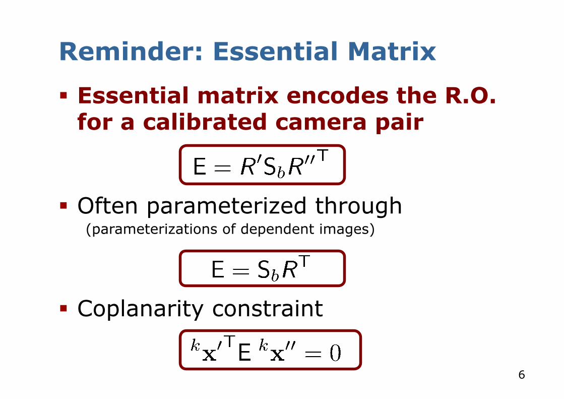
Reminder: Essential Matrix
§ Essential matrix encodes the R.O. for a calibrated camera pair
§ Often parameterized through
§ Coplanarity constraint
(parameterizations of dependent images)
7
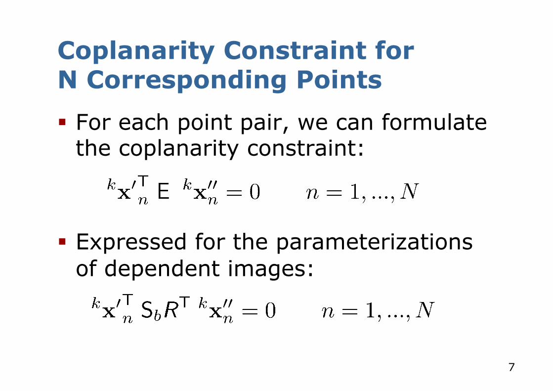
Coplanarity Constraint for N Corresponding Points § For each point pair, we can formulate
the coplanarity constraint:
§ Expressed for the parameterizations of dependent images:

8
Estimate the Essential Matrix (Here: Stereo Normal Case) § Estimate through least squares § Coplanarity constraint directly
yields an error function in the parameters of the R.O.
§ Coplanarity constraint is non-linear in the parameters
§ Thus, we need to iterate

9
Non-Linear Error Function
§ Coplanarity constraint yields a non-linear error function
Assumptions § Approximately stereo normal case § Classic photogrammetric parameteriz.
of dependent images ( , 5 parameters for the R.O.)
10
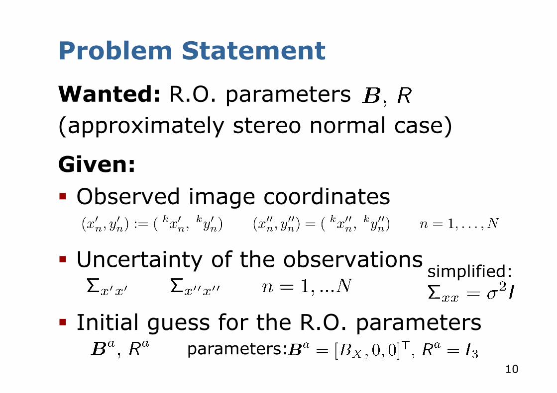
Problem Statement
Wanted: R.O. parameters (approximately stereo normal case)
Given: § Observed image coordinates
§ Uncertainty of the observations
§ Initial guess for the R.O. parameters parameters:
simplified:

11
Towards the Linearized Observation Equations § Starting point: § Initial guess: § Next goal: find the observation
equation for the Gauss-Markov model:
observation + correction = coefficients times corrections in unknowns

12
Towards the Linearized Observation Equations § Starting point: § Initial guess: § “How do variations in the parameters
effect the function itself?”
correction in x’
correction in x’’

13
Basis
§ Linearized equation for the basis
§ This leads to the skew-symmetric
2 unknowns
correction in Sb

14
Rotation
§ Linearized equation for the rotation
§ Coplanarity constraint (~normal case)
3 unknowns correction in R
15
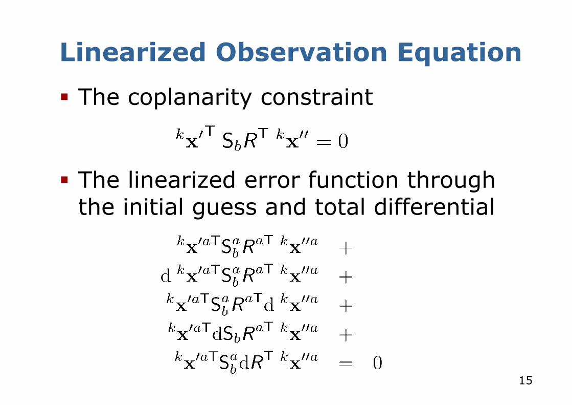
Linearized Observation Equation
§ The coplanarity constraint
§ The linearized error function through the initial guess and total differential
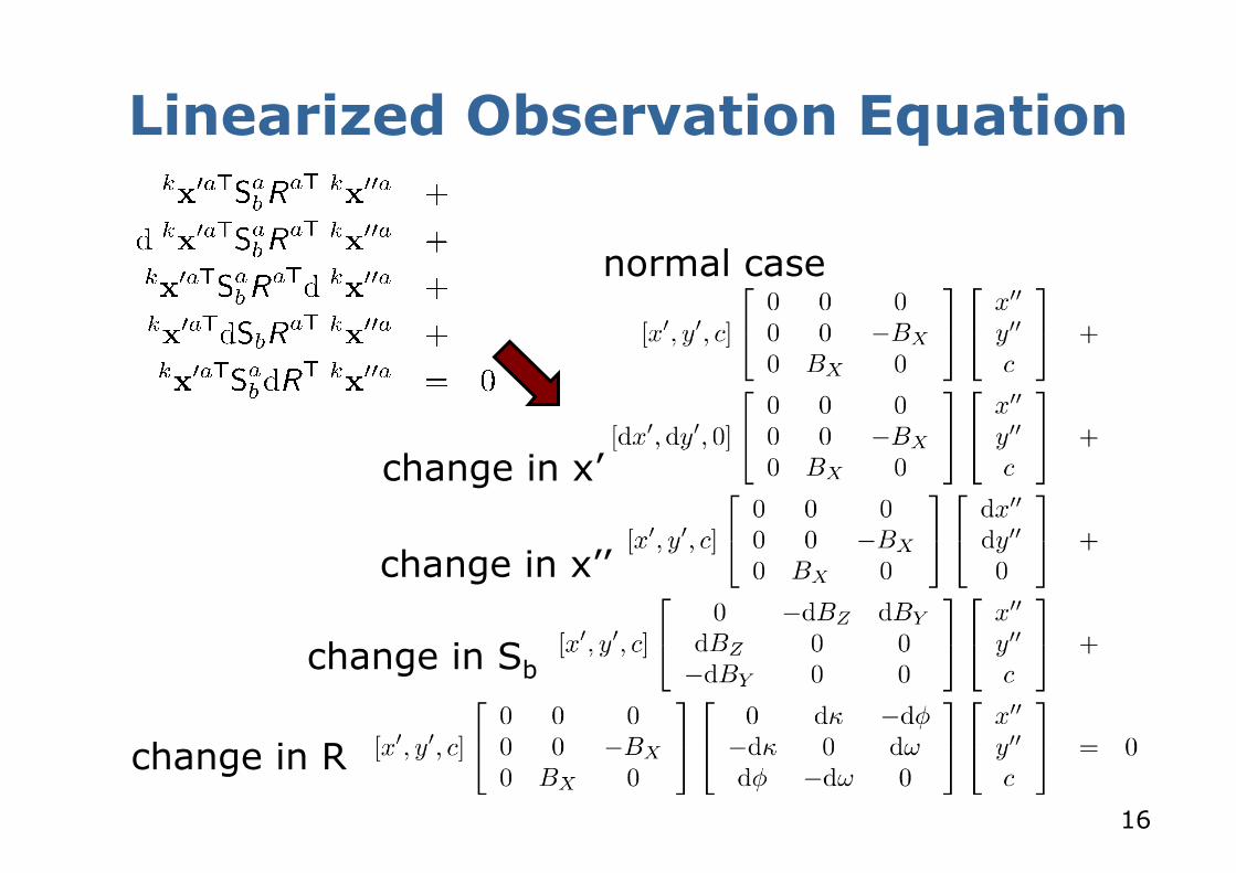
16
Linearized Observation Equation
change in x’’
change in Sb
change in R
change in x’
normal case

17
Linearized Observation Equation
change in x’’
change in Sb
change in R
change in x’
normal case
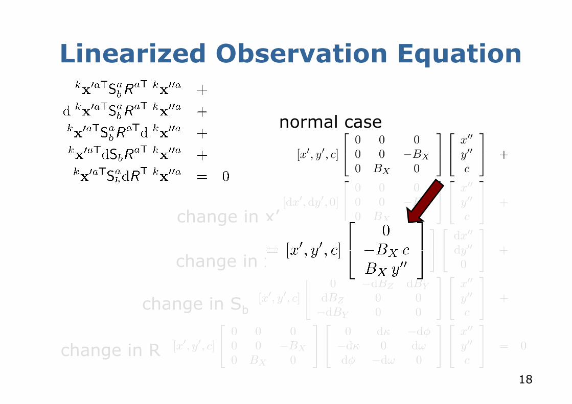
18
Linearized Observation Equation
change in x’’
change in Sb
change in R
change in x’
normal case

19
Linearized Observation Equation
change in x’’
change in Sb
change in R
change in x’
normal case

20
Linearized Observation Equation
change in x’’
change in Sb
change in R
change in x’
normal case
21
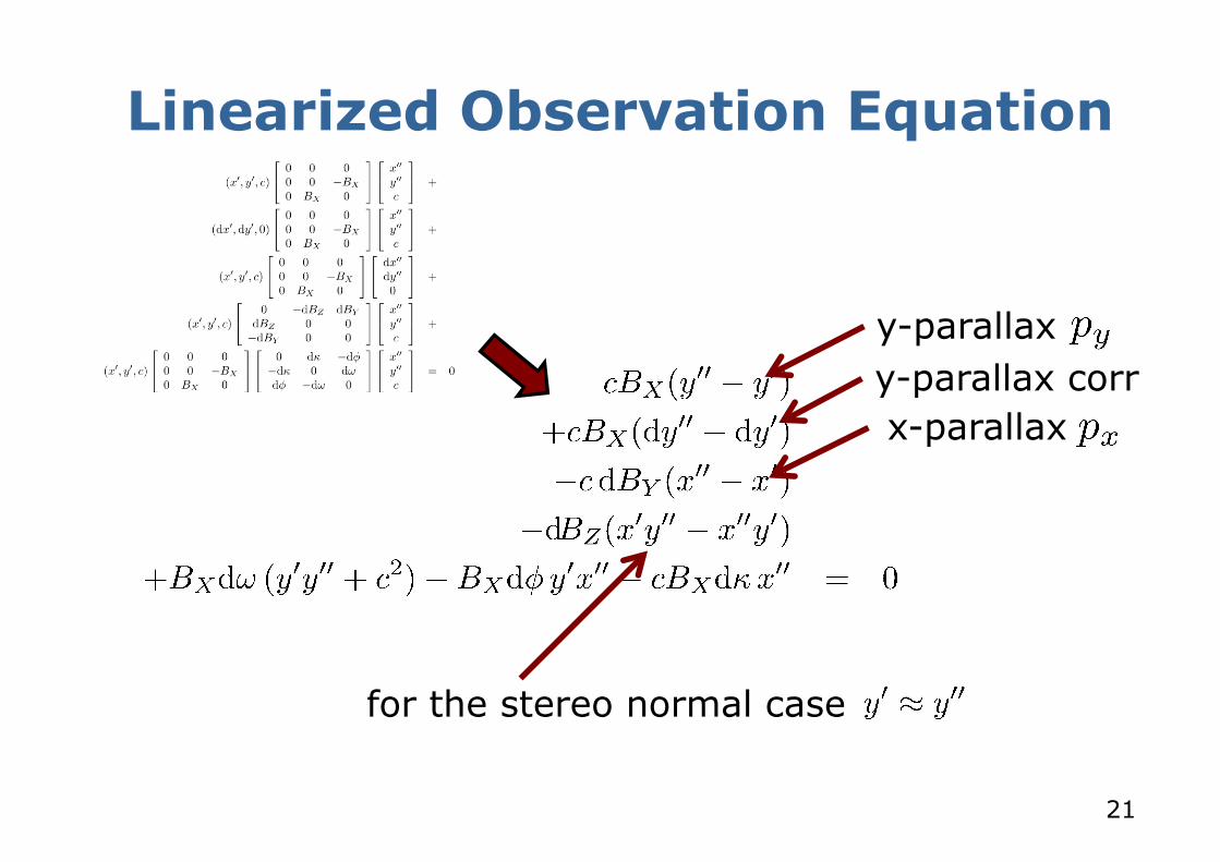
Linearized Observation Equation
for the stereo normal case
x-parallax
y-parallax y-parallax corr

22
Linearized Observation Equation Target py because this is the term to be zero (coplanarity constraint
for stereo normal)
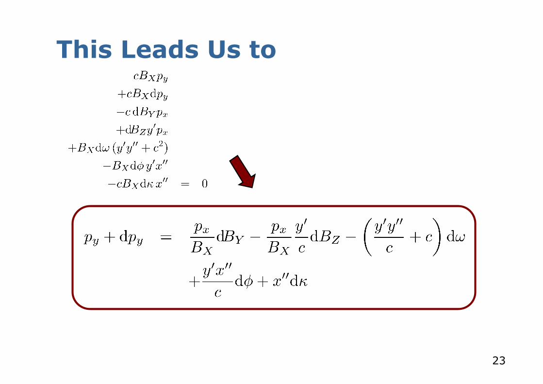
23
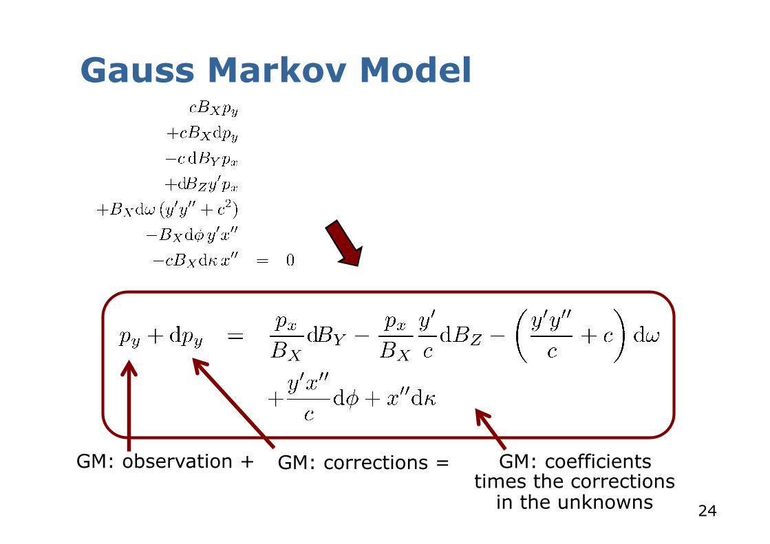
This Leads Us to
24
Gauss Markov Model
GM: observation + GM: corrections =
GM: coefficients times the corrections
in the unknowns

25
Observation Equation Written Using Vectors
coefficients times the corrections
in the unknowns

26
For All Observations, We Obtain
27
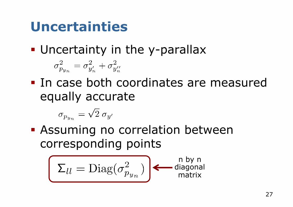
Uncertainties
§ Uncertainty in the y-parallax § In case both coordinates are measured
equally accurate
§ Assuming no correlation between corresponding points
n by n diagonal matrix
28
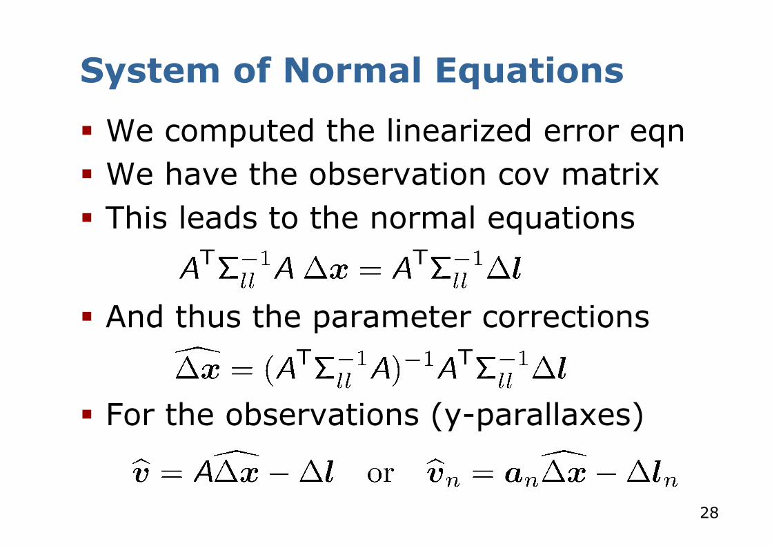
System of Normal Equations
§ We computed the linearized error eqn § We have the observation cov matrix § This leads to the normal equations
§ And thus the parameter corrections
§ For the observations (y-parallaxes)

29
Summary so far
§ Iterative least squares approach to estimate the relative orientation for calibrated cameras
§ We used the coplanarity constraint as our error function
§ Linearization § Yields GM model § Setup of a linear system § Solving it yields the corrections
30
Quality of the Result “How Good is a Solution?”

31
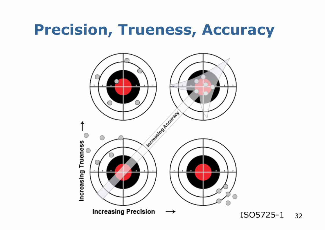
Precision, Trueness, Accuracy § Precision (DE: Präzision)
The closeness of agreement between independent test results obtained under the same conditions.
§ Trueness (DE: Richtigkeit) The closeness of agreement between the average value obtained from a large series of measurements and the true value.
§ Accuracy (DE: äußere Genauigk.) The closeness of agreement between a test result and the true value.
32
Precision, Trueness, Accuracy
ISO5725-1
33
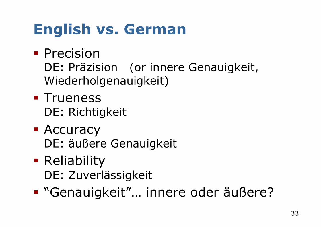
English vs. German § Precision
DE: Präzision (or innere Genauigkeit, Wiederholgenauigkeit)
§ Trueness DE: Richtigkeit
§ Accuracy DE: äußere Genauigkeit
§ Reliability DE: Zuverlässigkeit
§ “Genauigkeit”… innere oder äußere?

34
Precision for the Relative Orientation
§ Precision: How large is the influence of random noise on the result?
35
Precision & Reliability for the Relative Orientation
§ Precision: How large is the influence of random noise on the result?
§ Reliability: Can we detect measurement errors/outliers?

36
Precision
§ To analyze the precision, we need the covariance matrix of the unknowns
§ Theoretical precision
§ Empirical precision
§ Empirical and theoretical precision related through the variance factor

37
Variance Factor
§ Computation of the variance factor
§ Weighted sum of the squared corrections in the parallaxes after convergence
§ Redundancy

38
Empirical Precision
§ With a redundancy of R>30, we obtain realistic estimates of the precision of our unknown relative orientation

39
Correlation
§ We can also compute the correlation of the parameters
§ Large correlation values (=> +1/-1) between parameters can be a reason for instabilities of the solution

40
Reliability
§ Covariance matrix of the corrections
§ is smaller than § Redundancy components of
observations are defined as
§ Sum over all gives the redundancy

41
Reliability
§ Redundancy components tells which fraction of original errors we see in the residual parallaxes after the adjustment
§ Small values for indicate that outliers are hard to detect

42
Quality of the Relative Orientation
for the Stereo Normal Case
43
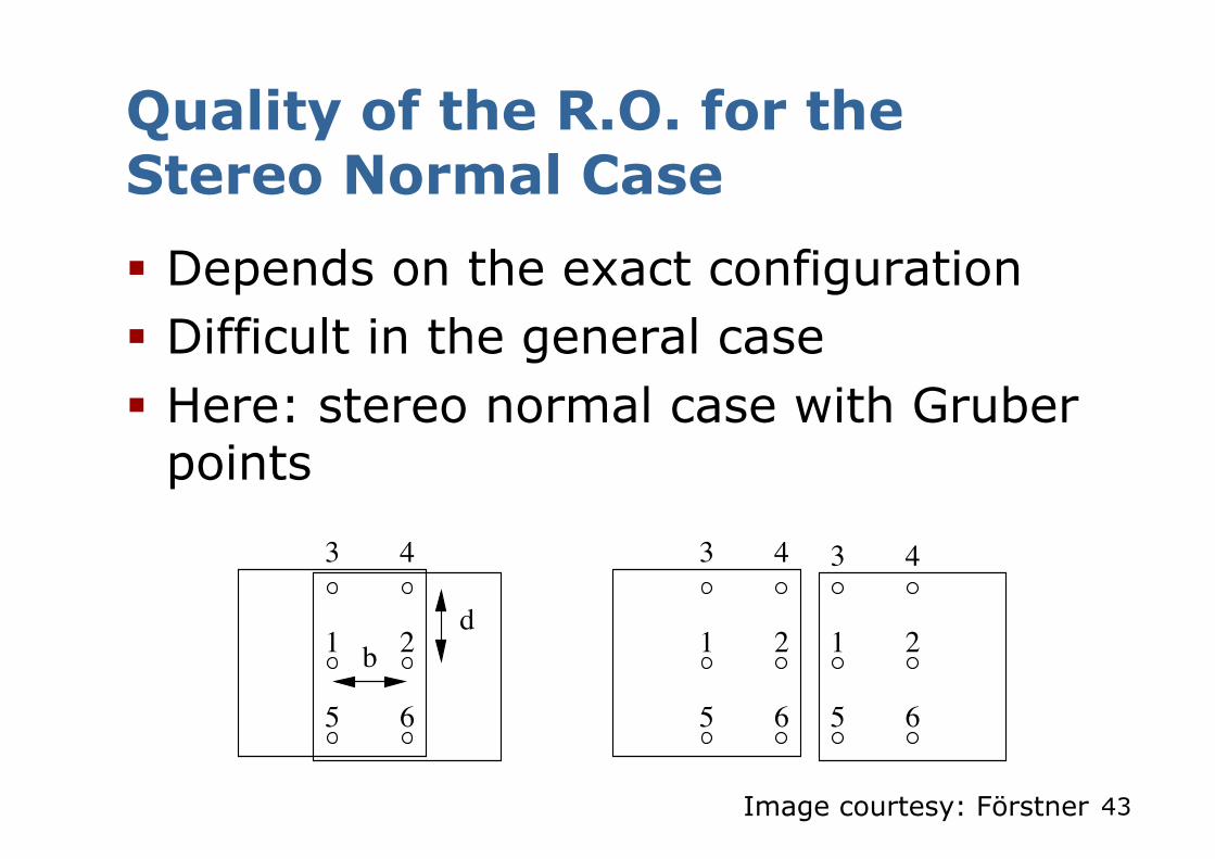
Quality of the R.O. for the Stereo Normal Case § Depends on the exact configuration § Difficult in the general case § Here: stereo normal case with Gruber
points
Image courtesy: Förstner
1 2
3 4
5 6
1,1’ 2,2’
3,3’ 4,4’
6,6’5,5’
2
3 4
5 6
1 2
3 4
65
1
6,6’
2,2’
4,4’3,3’
1,1’ 2,2’
3,3’ 4,4’
5,5’ 6,6’5,5’
1,1’
bd

44
Assumptions
§ Six corresponding points (Gruber points) in the overlapping area
§ Image overlap: 60% § Identical uncertainty in y-parallaxes
(weight=1, ) § Basis (image scale number
times image basis)
1 2
3 4
5 6
1,1’ 2,2’
3,3’ 4,4’
6,6’5,5’
2
3 4
5 6
1 2
3 4
65
1
6,6’
2,2’
4,4’3,3’
1,1’ 2,2’
3,3’ 4,4’
5,5’ 6,6’5,5’
1,1’
bd
Image courtesy: Förstner

45
Image Coordinates
1 2
3 4
5 6
1,1’ 2,2’
3,3’ 4,4’
6,6’5,5’
2
3 4
5 6
1 2
3 4
65
1
6,6’
2,2’
4,4’3,3’
1,1’ 2,2’
3,3’ 4,4’
5,5’ 6,6’5,5’
1,1’
bd
Image courtesy: Förstner

46
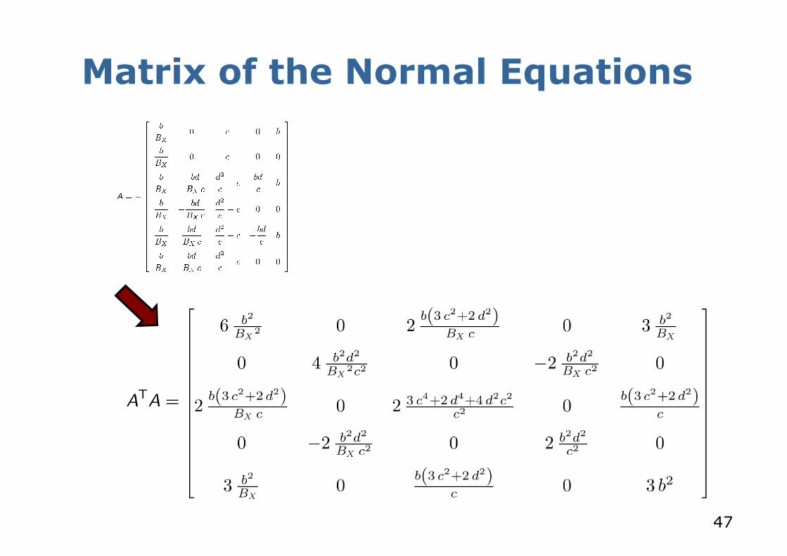
Coefficient Matrix
point 1
point 6
…
47
Matrix of the Normal Equations
48
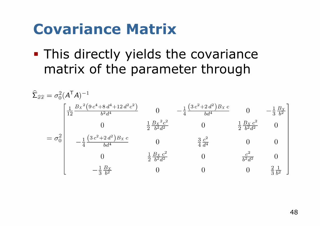
Covariance Matrix
§ This directly yields the covariance matrix of the parameter through
49
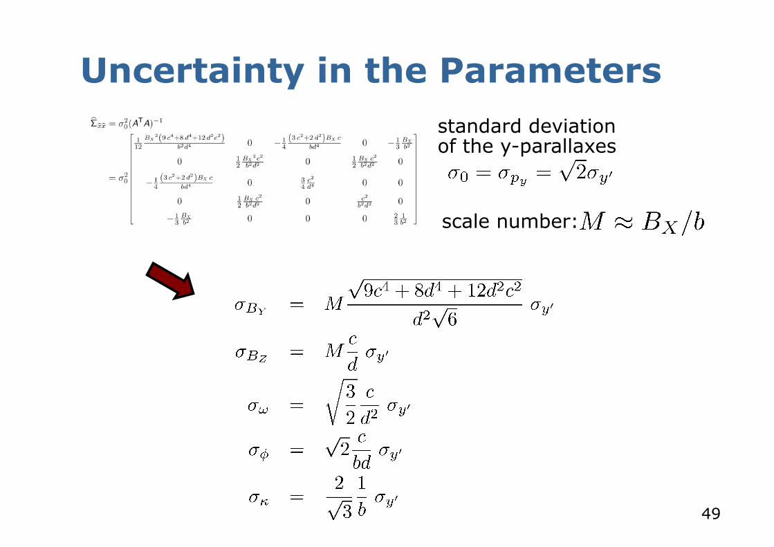
Uncertainty in the Parameters standard deviation of the y-parallaxes
scale number:

50
Discussion
§ Impact of the pixel measurements
“the more accurate one can measure the parallaxes, the better the result

51
Discussion
§ Size of the scene and overlap
“the larger the scene and the overlap, the better the result
1 2
3 4
5 6
1,1’ 2,2’
3,3’ 4,4’
6,6’5,5’
2
3 4
5 6
1 2
3 4
65
1
6,6’
2,2’
4,4’3,3’
1,1’ 2,2’
3,3’ 4,4’
5,5’ 6,6’5,5’
1,1’
bd

52
Discussion
“the spread of the points in the plane (b, d) strongly impacts roll and pitch”
1 2
3 4
5 6
1,1’ 2,2’
3,3’ 4,4’
6,6’5,5’
2
3 4
5 6
1 2
3 4
65
1
6,6’
2,2’
4,4’3,3’
1,1’ 2,2’
3,3’ 4,4’
5,5’ 6,6’5,5’
1,1’
bd
§ Size of the scene and overlap

53
Discussion
§ Camera constant
“the smaller the camera constant (at identical images), the better the result

54
Discussion
§ Scale number and the baseline
image scale number:
“the smaller the image scale number (or the larger the image scale), the better the resulting baseline

55
Discussion
§ All quantities are proportional to § increase with the scale number § d strongly influences
roll ( ) and pitch ( ) § If , all quantities
become more accurate with a larger basis
§ The more the overlap is exploited, the better
1 2
3 4
5 6
1,1’ 2,2’
3,3’ 4,4’
6,6’5,5’
2
3 4
5 6
1 2
3 4
65
1
6,6’
2,2’
4,4’3,3’
1,1’ 2,2’
3,3’ 4,4’
5,5’ 6,6’5,5’
1,1’
bd

56
Reliability
§ Covariance matrix of the corrections
§ and thus the redundancy components
57
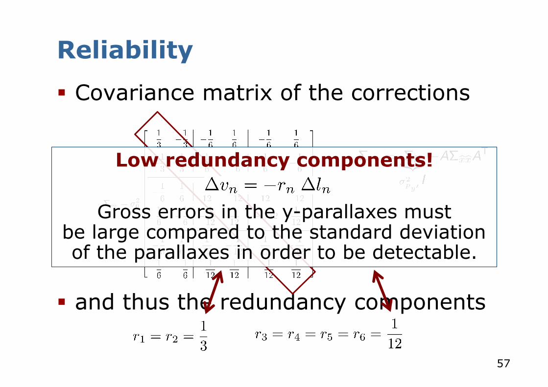
Reliability
§ Covariance matrix of the corrections
§ and thus the redundancy components
Low redundancy components!
Gross errors in the y-parallaxes must be large compared to the standard deviation of the parallaxes in order to be detectable.

58
Double Points/12 Gruber Points
Improving the result with 12 points
1 2
3 4
5 6
1,1’ 2,2’
3,3’ 4,4’
6,6’5,5’
2
3 4
5 6
1 2
3 4
65
1
6,6’
2,2’
4,4’3,3’
1,1’ 2,2’
3,3’ 4,4’
5,5’ 6,6’5,5’
1,1’
bd

59
Double Points
Improving the result with 12 points
1 2
3 4
5 6
1,1’ 2,2’
3,3’ 4,4’
6,6’5,5’
2
3 4
5 6
1 2
3 4
65
1
6,6’
2,2’
4,4’3,3’
1,1’ 2,2’
3,3’ 4,4’
5,5’ 6,6’5,5’
1,1’
bd
no. points
Furthermore: The more points we have, the easier we can detect outliers!

60
Double Points
Covariance of the parallax corrections which leads to the redundancy components

61
Double Points
Covariance of the parallax corrections which leads to the redundancy components
Outliers are much easier to detect with Gruber “double” points!

62
Double Points
Covariance of the parallax corrections which leads to the redundancy components
Outliers are much easier to detect with Gruber “double” points!
The more points we have, the easier we can detect outliers!

63
Summary
§ Estimating the relative orientation using a least squares approach
§ Solution for the normal stereo case (done without relinearizing)
§ Statistically optimal solution § Analysis of the solution based on
Gruber points § More points improve the results

64
Literature
§ Förstner, Skript Photogrammetrie II, Chapter 1.3
§ Förstner, Wrobel: Photogrammetric Computer Vision, Ch. 12.3.6 & 3.3.3

65
Slide Information § These slides have been created by Cyrill Stachniss as part of
the Photogrammetry II course taught in 2014/15. § The material heavily relies on the very well written scripts by
Wolfgang Förstner and the (upcoming) Photogrammetric Computer Vision book by Förstner and Wrobl.
§ I tried to acknowledge all people that contributed image or video material. In case I missed something, please let me know. If you adapt this course material, please make sure you keep the acknowledgements.
§ Feel free to use and change the slides. If you use them, I would appreciate an acknowledgement as well. To satisfy my own curiosity, please send me short email notice.
Cyrill Stachniss, 2014


