0

Iterative Timing Recovery

John R. Barry

School of Electrical and Computer Engineering, Georgia TechAtlanta, Georgia U.S.A.barry@ece.gatech.edu

1

Outline

Timing Recovery Tutorial

• Problem statement• TED: M&M, LMS, S-curves• PLL

Iterative Timing Recovery

• Motivation (powerful FEC)• 3-way strategy• Per-survivor strategy• Performance comparison

2

0 T 2T 5T

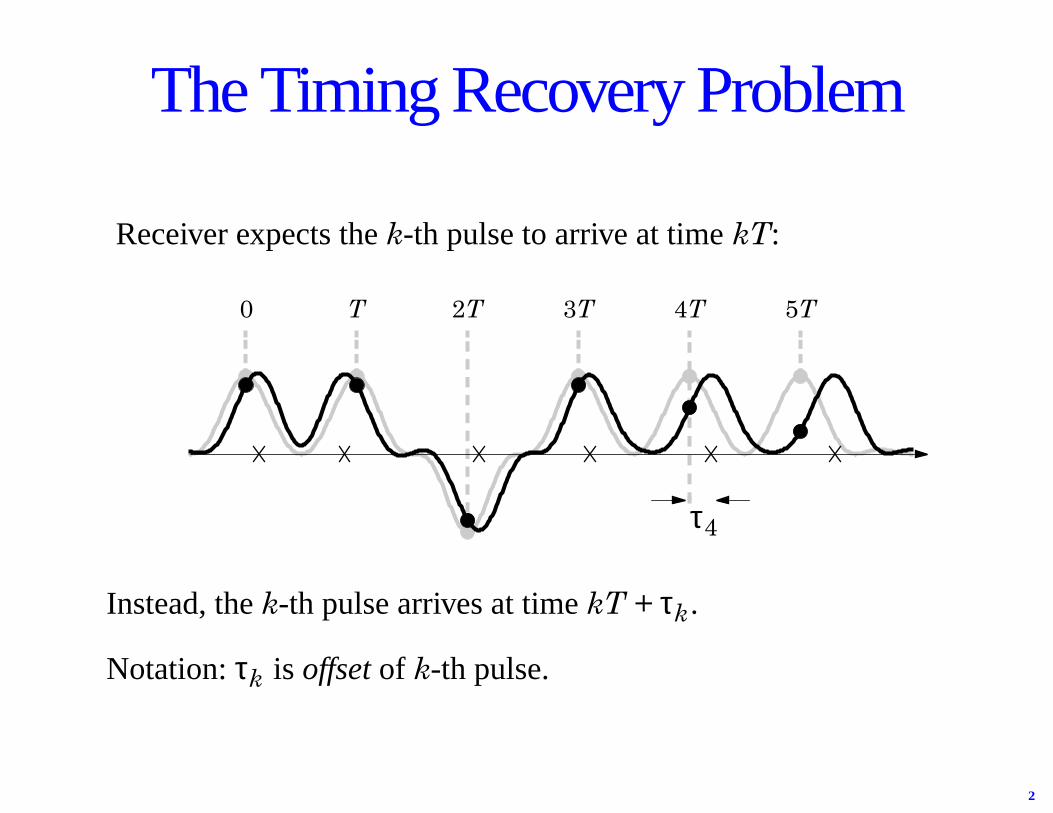
Receiver expects the k-th pulse to arrive at time kT:

3T 4T

Instead, the k-th pulse arrives at time kT + τk .

The Timing Recovery Problem

τ4

Notation: τk is offset of k-th pulse.

3

TIMINGRECOVERY

r( t )

kT + kτ

to digitaldetector

Sampling

Best sampling times are{kT + τk}.

Estimate{τk}

4

Timing Offset Models

CONSTANT

FREQUENCY OFFSET

RANDOM WALK

TIME

TIME

TIME

τk

τk

τk

⇒

⇒

⇒τk+1 = τk + N (0, σw2 )

RANDOM WALK + FREQUENCY OFFSET

τk+1 = τk + N (∆T, σw2 )

τk = τ0

τk+1 = τk + ∆T

5

The PR4 Model and Notation

TIMINGOFFSETS

ak r( t ) = ∑kdk g(t – kT – τk)g(t)

AWGNdk

τ1 – D2

2T 4T–2T 0

Define: • dk = ak – ak – 2 ∈{0, ±2} = 3-level “PR4” symbol

• k = receiver’s estimate ofdk

• τk = timing offset

• k = receiver’s estimate ofτk

• εk = τk – k estimate error, with stdσε.

• k = receiver’s estimate ofεk

d

ττ

ε

+ AWGN∈{±1} ∈{0, ±2}SINC FUNCTION

6

ML Estimate: Trained, Constant Offset

The ML estimate minimizes J( |a) = r( t ) – dig(t – iT – τ) dt .

Exhaustive search:

Try all values forτ, pick one that best representsr( t ) in MMSE sense.

τ τ∞–

∞∫

i∑

2

–2T –T 0 T 2T

J

τ

7

ANIMATION 1

8

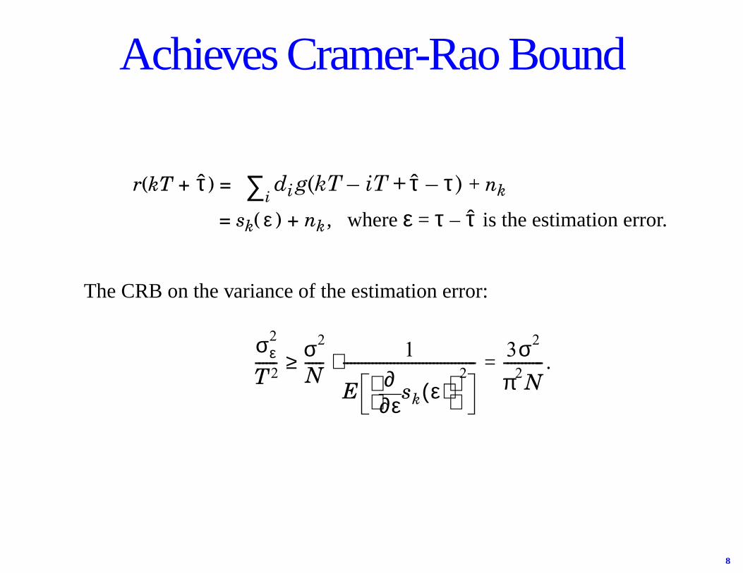
r(kT + ) = di g(kT – iT + – τ) + nk

= sk( ε ) + nk, whereε = τ – is the estimation error.

The CRB on the variance of the estimation error:

≥ = .

τi∑ τ

τ

σε2

T2------ σ2

N----- 1

Eε∂

∂ sk ε( ) 2

-------------------------------------⋅ 3σ2

π2N-----------

Achieves Cramer-Rao Bound

9

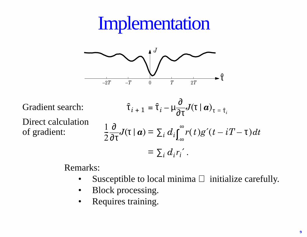
Gradient search: i + 1 = i – µ J(τ|a)

Direct calculationof gradient: J(τ|a) = r( t )g´(t – iT – τ)dt

= ri´ .

Remarks:• Susceptible to local minima⇒ initialize carefully.• Block processing.• Requires training.

τ τ τ∂∂

τ τi=

12---

τ∂∂ ∑i di

∞–

∞∫

∑i di

Implementation

–2T –T 0 T 2T

J

τ

10

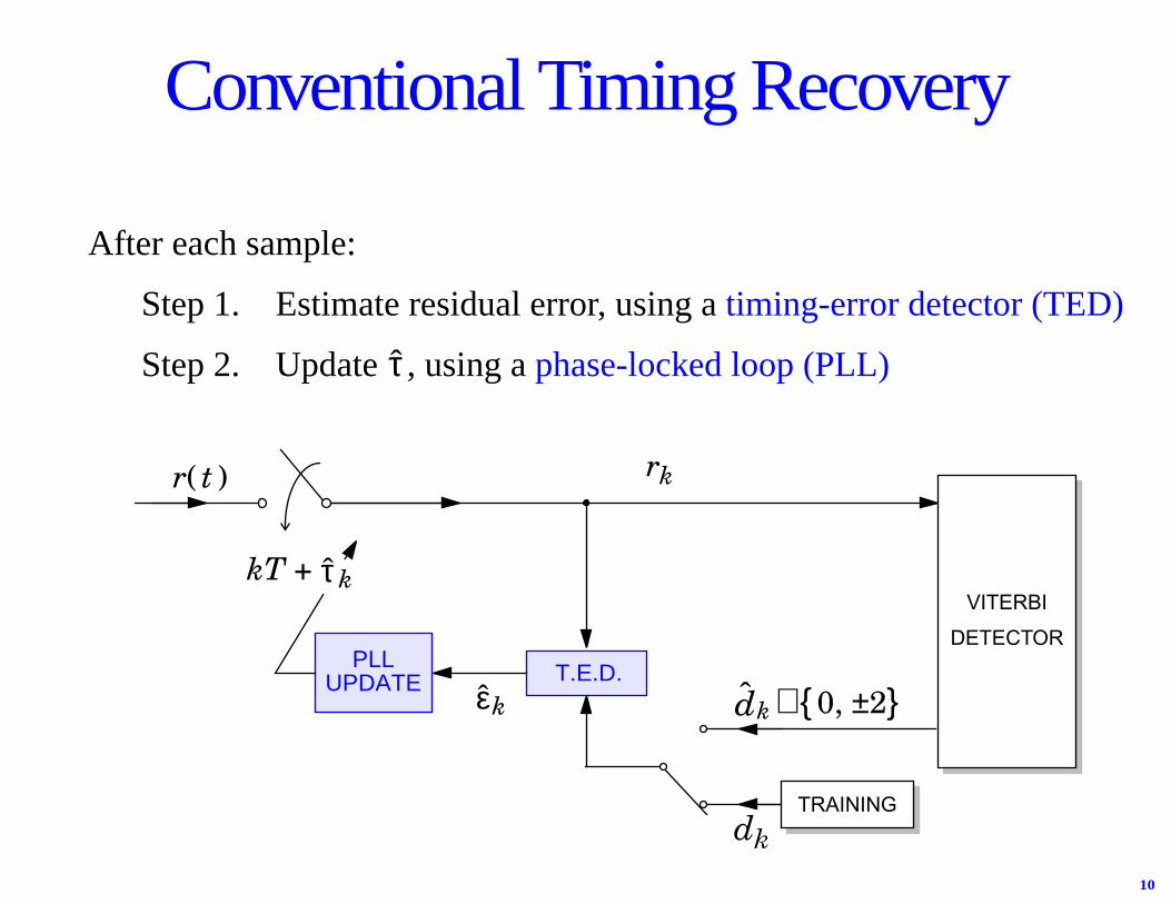
PLLUPDATE

r( t )

T.E.D.

kT + kτ

rk

∈{0, ±2}kε

Conventional Timing Recovery

After each sample:

Step 1. Estimate residual error, using a timing-error detector (TED)

Step 2. Update , using a phase-locked loop (PLL)τ

TRAININGdk

dk

VITERBI

DETECTOR

11

LMS Timing Recovery

MMSE cost function:

E rk – dk

2

LMS approach: k + 1 = k + µ k

where = – rk – dk .

τ τ ε

εk τ∂∂

2

τ τk=

what we want it to bek-th sample,rk = r(kT + k)τ

12

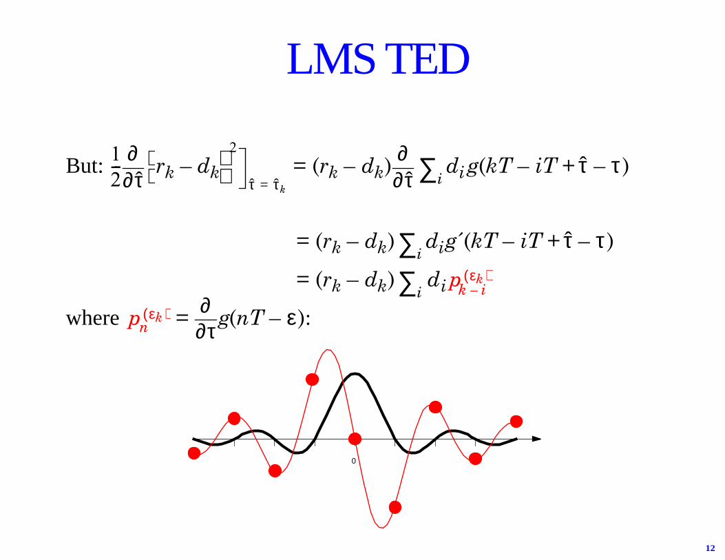
But: rk – dk = (rk – dk) di g(kT – iT + – τ)

= (rk – dk) dig´(kT – iT + – τ)

= (rk – dk) di

where = g(nT – ε):

12---

τ∂∂

2

τ τk= τ∂∂

i∑ τ

i∑ τ

i∑ pk i–εk( )

pnεk( )

τ∂∂

0

LMS TED

13

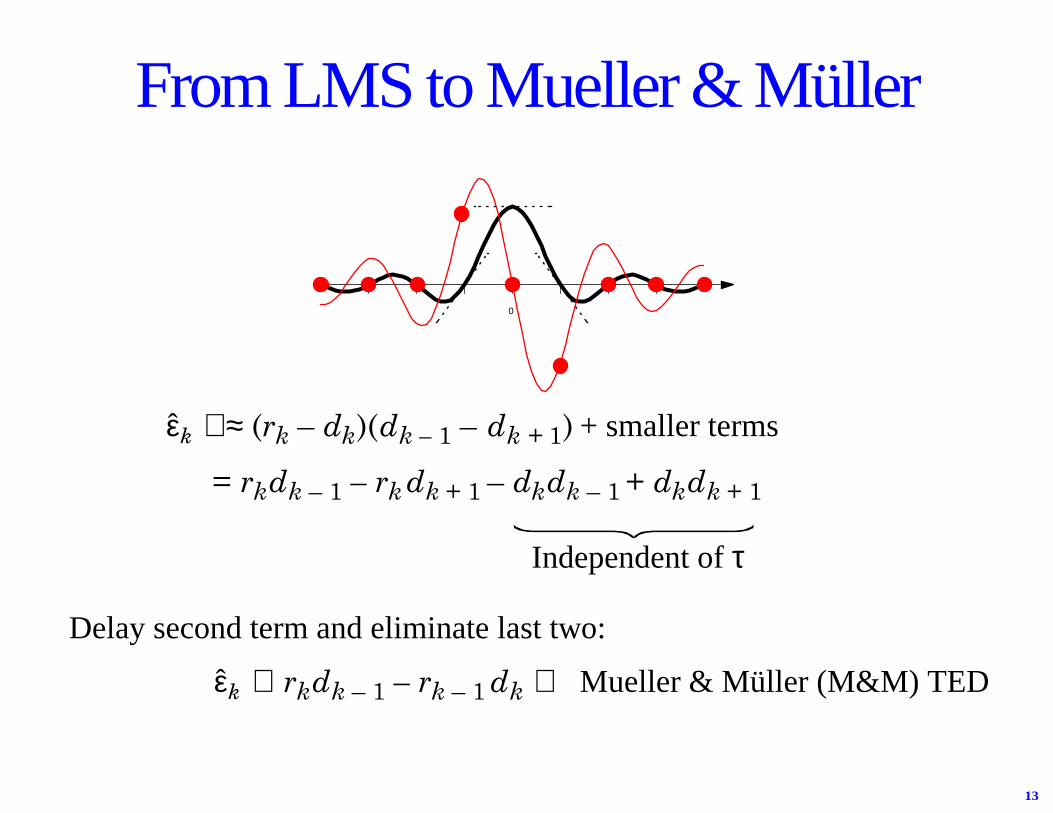
From LMS to Mueller & Müller

0

∝≈ (rk – dk)(dk – 1 – dk + 1) + smaller terms

= rkdk – 1 – rk dk + 1 – dkdk – 1 + dkdk + 1

Delay second term and eliminate last two:

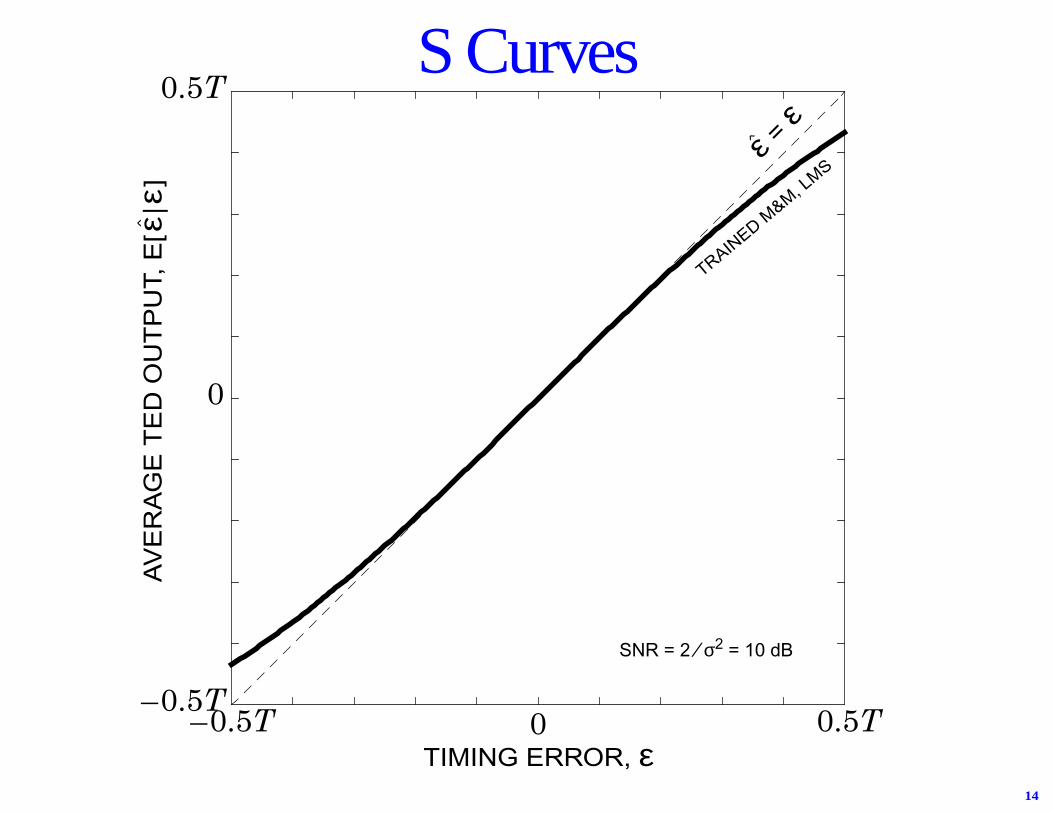
∝ rkdk – 1 – rk – 1 dk ⇒ Mueller & Müller (M&M) TED

εk

Independent ofτ

εk

14

–0.5T 0 0.5T–0.5T

0

0.5TS Curves

TIMING ERROR, ε

AV

ER

AG

E T

ED

OU

TP

UT,

E[ε

|ε]

^

TRAINED M

&M, LMS

ε =ε

^

SNR = 2 ⁄ σ2 = 10 dB

15

–0.5T 0 0.5T–0.5T

0

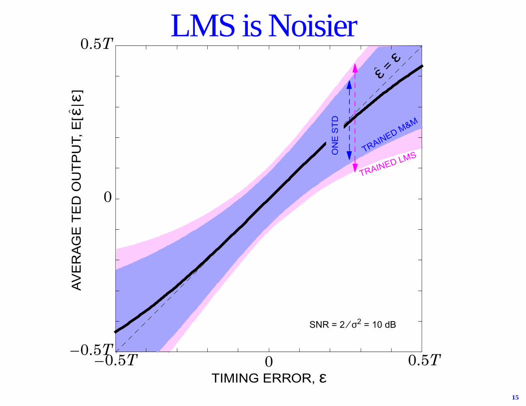
0.5TLMS is Noisier

TIMING ERROR, ε

AV

ER

AG

E T

ED

OU

TP

UT,

E[ε

|ε]

^

TRAINED M&M

ε =ε

^

TRAINED LMSON

E S

TD

SNR = 2 ⁄ σ2 = 10 dB

16

An Interpretation of M&M

• It passes through {0, ±2, ±2 ± 2j, ±2j} at times {kT + τ}.

• More often than not, in a counterclockwise direction.

0 2

–2

0

2

–2

Consider the complex signal r( t ) + jr(t – T).Its noiseless trajectory:

17

ANIMATION 2

18

Sampling Late by 20%Rk = rk + jrk – 1

Dk = dk + jdk – 1θ

The angle betweenRk andDk predicts timing error:

θ ≈ sinθ = Im ∝ rkdk – 1 – rk – 1dk ¶⇒ M&M.R*DRD

----------------

19

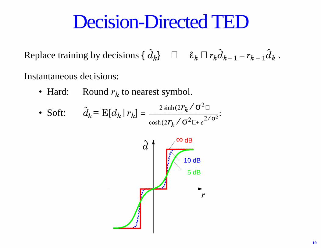
Decision-Directed TED

Replace training by decisions { k} ⇒ k ∝ rk k – 1 – rk – 1 k .

Instantaneous decisions:

• Hard: Round rk to nearest symbol.

• Soft: k = E[dk|rk] = :

d ε d d

d2 2rk σ2⁄( )sinh

2rk σ2⁄( )cosh e2 σ2⁄+

----------------------------------------------------------------

5 dB

10 dB

∞ dB

r

d

20

–0.5T 0 0.5T–0.5T

0

0.5T

TIMING ERROR, ε

AV

ER

AG

E T

ED

OU

TP

UT,

E[ε

|ε]

^

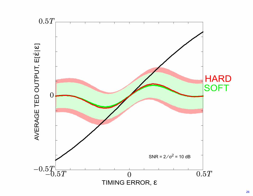
HARD M&M

SOFT M&M

TRAINED M

&M, LMS

SNR = 2 ⁄ σ2 = 10 dB

21

–0.5T 0 0.5T–0.5T

0

0.5T

TIMING ERROR, ε

AV

ER

AG

E T

ED

OU

TP

UT,

E[ε

|ε]

^

HARDSOFT

SNR = 2 ⁄ σ2 = 10 dB

22

DECODERTRELLIS

EQUALIZER

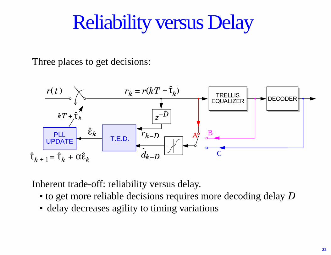
Reliability versus Delay

Three places to get decisions:

kT + kτ

r( t )DECODER

dk–D= + ατk 1+ τk εk

A B

C

rk = r(kT + k)TRELLIS

EQUALIZER

z–D

τ

rk–DPLLUPDATE T.E.D.

kε

Inherent trade-off: reliability versus delay.• to get more reliable decisions requires more decoding delayD• delay decreases agility to timing variations

23

Decision Delay Degrades Performance

0 0.02 0.04 0.06 0.08 0.12.5

3

3.5

4

4.5

5

5.5

PLL GAIN, α

RM

S T

IMIN

G J

ITT

ER

σ ε⁄T

(%)

D=

20

D=

10

D= 5

D = 0

D=

15Eb ⁄ N0 = 8 dBσw ⁄ T = 0.5%

TRAINED M&M1st-ORDER PLL

24

Averaged over 40,000 bits

Parameters

1st-order M&M PLLrandom walk σw ⁄ T = 0.5%

α optimized for SNR = 10 dB

0 5 10 15 20 251%

2%

3%

4%

5%

6%

7%

SNR (dB)

The Instantaneous-vs-Reliable Trade-Off

INSTANTANEOUS BUT

20 0.017100 0.006

0 0.046

Delay αopt

UNRELIABLE DECISIONS

DELAY-20,PERFECT DECISIONS

DELAY-100,PERFECT DECISIONS

Reliability becomes moreimportant at low SNR.

σε ⁄ TJITTER

25

αz 1–

1 1 α–( )z 1––-----------------------------------

Linearized Analysis

Assume = εk + independent noise= τk – k + nk

⇒1st order PLL, k + 1 = k + α(τk – k + nk), is a linear system:

εkτ

τ τ τ

τk

NOISE

τk

1-st order LPF

Ex: Random walk

αz 1–

1 1 α–( )z 1––-----------------------------------

τk τk

1-st order LPF

11 z 1––-----------------

wkWHITE

WHITE

⇒ derive optimal α

εk+– to minimize σε

2

α

26

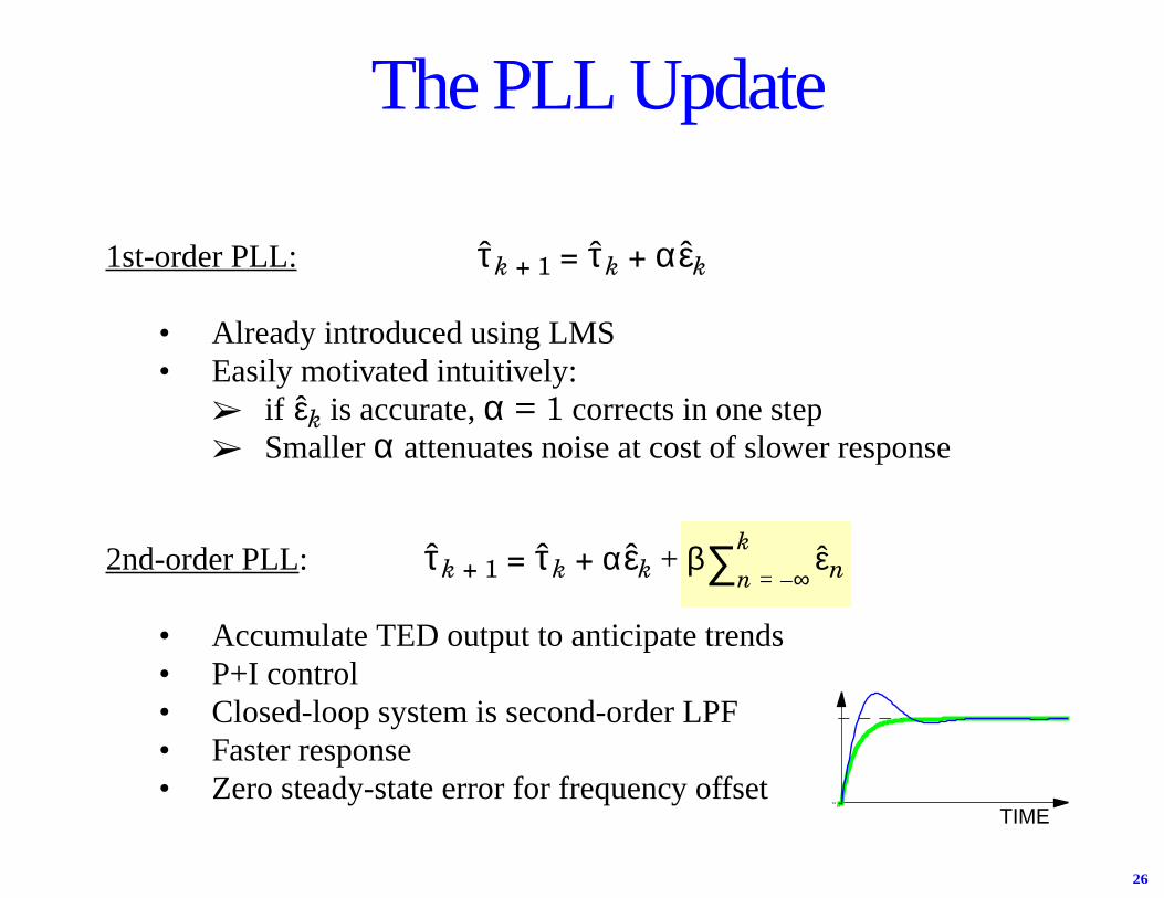
1st-order PLL: k + 1 = k + α k

• Already introduced using LMS• Easily motivated intuitively:

➢ if k is accurate, α = 1 corrects in one step➢ Smaller α attenuates noise at cost of slower response

2nd-order PLL: k + 1 = k + α k + β n

• Accumulate TED output to anticipate trends• P+I control• Closed-loop system is second-order LPF• Faster response• Zero steady-state error for frequency offset

τ τ ε

ε

τ τ ε εn ∞–=

k∑

The PLL Update

00

TIME

27

Equivalent Views of PLL

Analysis: Sample at {kT + k}, where

• k + 1 = k + α k + β n ,

• k is estimate of timing error at time k .

Implementation:

τ

τ τ ε εn ∞–=

k∑ε

PHASE DETECTORLOOP FILTER

TEDVCO

A ⁄ D

α β1 z 1––----------------+

εk

Accumulationimplicit in VCO

28

Iterative Timing Recovery

Motivation

• Powerful codes⇒ low SNR⇒ timing recovery is difficult

• traditional PLL approach ignores presence of code

Key Questions

• How can timing recovery exploit code?

• What performance gains can be expected?

• Is it practical?

29

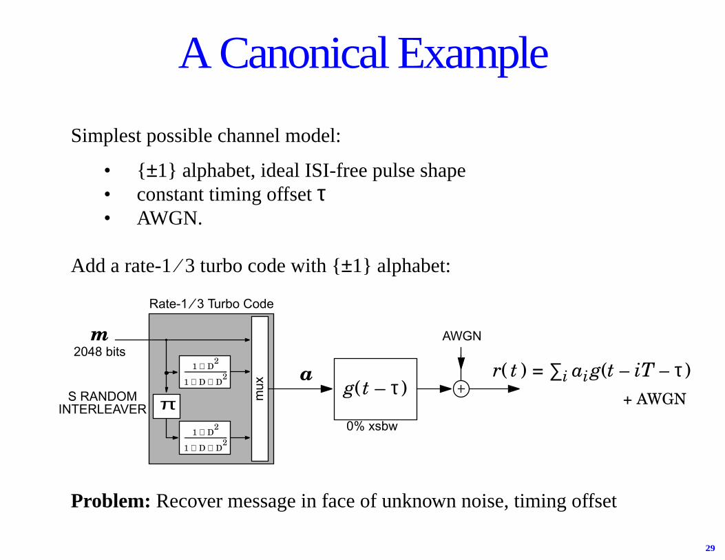
A Canonical Example

m

mux

AWGN

S RANDOM

Rate-1 ⁄ 3 Turbo Code

r( t ) = ∑i ai g(t – iT – τ)g(t – τ)

π0% xsbw

a

Simplest possible channel model:

• { ±1} alphabet, ideal ISI-free pulse shape• constant timing offsetτ• AWGN.

Add a rate-1⁄ 3 turbo code with {±1} alphabet:

INTERLEAVER

1 D2

⊕

1 D D2

⊕ ⊕-------------------------------

1 D2

⊕

1 D D2

⊕ ⊕-------------------------------

+ AWGN

Problem: Recover message in face of unknown noise, timing offset

2048 bits

30

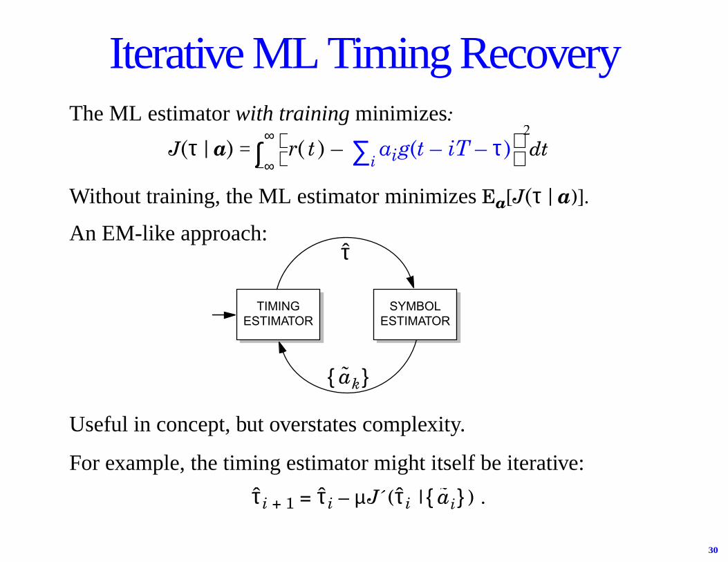
The ML estimatorwith training minimizes:

J( |a) = r( t ) – aig(t – iT – τ) dt

Without training, the ML estimator minimizesEa[J( |a)].

An EM-like approach:

τ∞–

∞∫

i∑

2

τ

Iterative ML Timing Recovery

ak{ }

SYMBOLESTIMATOR

τ

TIMINGESTIMATOR

Useful in concept, but overstates complexity.

For example, the timing estimator might itself be iterative:

i + 1 = i – µJ´ ( i | ) .τ τ τ ai{ }

31

A Reduced-Complexity Approach

Collapse three loops to a single loop.

Initialize 0

Iterate for i = 0, 1, 2, …

decode component 1

decode component 2

update timing estimate, i + 1 = i – µJ´ ( i | )

interpolate

end

As a benchmark, an iterative receiver that ignores the presence of FEC willreplace the pair of decoders by = tanh .

τ

τ τ τ ai{ }

aki( ) r kT τi+( )( ) σ2⁄( )

32

S = 16 random interleaver, length 2048

RM

S T

IMIN

G E

RR

OR

,σ ε

⁄T IGN

OR

E FEC4 dB

EX

PLO

IT F

EC

Trained ML,

Parameters

τ = 0.123T, AWGN channelRate-1 ⁄ 3 Turbo Code

N = 6150 coded bits

1 inner per outer iteration

K = 2048 message bits

Averaged over 180 trials0 5 10 15

0.2%

Eb ⁄ N0 (dB)

0.3%

0.4%

0.5%

1%

2%

3%

4%

5%

σε2 = E[( – )2]τ τ

Results

Cramer-Rao Bound

33

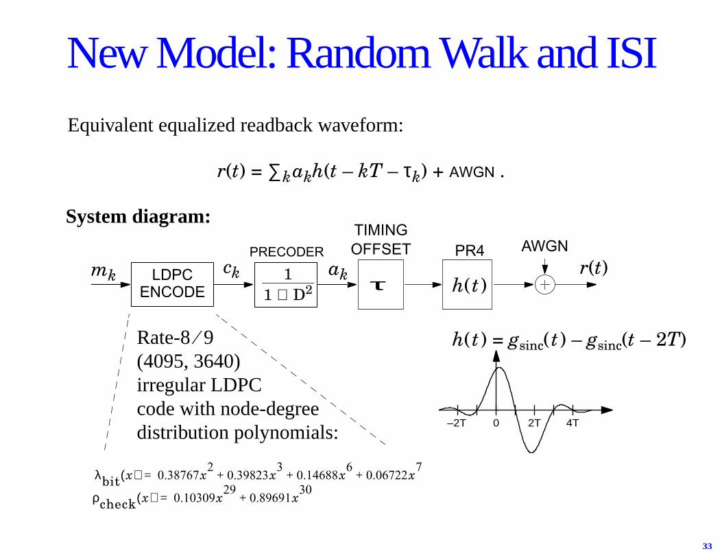
New Model: Random Walk and ISI

PRECODER

λbit x( ) 0.38767x20.39823x3

0.14688x60.06722x7

+ + +=

ρcheck x( ) 0.10309x290.89691x30

+=

mk akckLDPCENCODE

11 ⊕ D2 τ

r(t)

Rate-8⁄ 9(4095, 3640)irregular LDPCcode with node-degreedistribution polynomials:

h(t)

AWGNPR4TIMINGOFFSET

2T 4T–2T 0

Equivalent equalized readback waveform:

r(t) = ∑kakh(t – kT – τk) + AWGN .

h(t) = gsinc(t) – gsinc(t – 2T)

System diagram:

34

Conventional Turbo Equalizer + PLL

BCJR

PR trellis

–

+

–+

apriori

finaldecisions

PLL

BITNODES

CHECKNODES

kT τk+

λk

r(t)

= LLR(ck)

rk

35

Performance of Conventional Approach

4 5 6 7 810–6

10–5

10–4

10–3

10–2

10–1

1

SNR per bit (dB)

WO

RD

-ER

RO

RR

AT

E

σw ⁄T = 0.5% (α = 0.04)

σw ⁄T = 1% (α = 0.055)

KNOWN TIMING

Conventional: 25 ⁄ 5

Parameters

Known Timing: 10 ⁄ 5

max 10000000 words Big penalty as σw ⁄T increases: cycle slips.

36

Cycle-Slip Example

σw ⁄T = 1.0%

Parameters

SNRbit = 5.0 dB

0 2050 4100– 1.5T

–T

0

T

TIME k (in bit periods)

ES

TIM

AT

E O

F T

IMIN

G O

FF

SE

T(

)

ACTUAL τk

τ k

α = 0.055

T

τkCYCLESLIP

ESTIMATE

37

Nested Loops

BCJRPLLr(t)

τk{ }

LLR dk( ){ }

TURBO EQUALIZER

LLR ck( ){ }

LLR ck( ){ }

BITNODES

LDPC DECODER

EQ

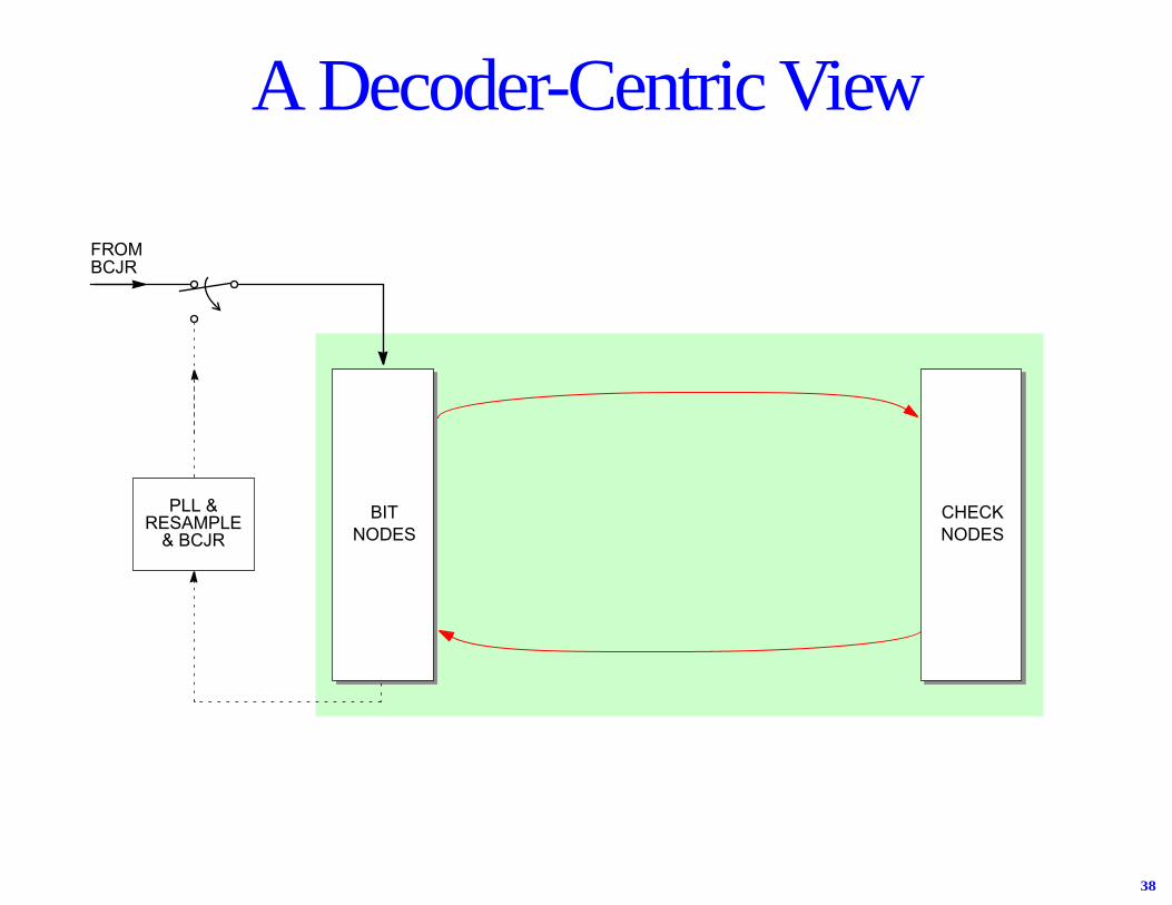
Iterate between PLL and turbo equalizer, which in turniterates between BCJR and LDPC decoder, which in turniterates between bit nodes and check nodes.

CHECKNODES

38

A Decoder-Centric View

BITNODES

PLL &RESAMPLE

& BCJR

FROMBCJR

CHECKNODES

39

CHECKNODES

BITNODES

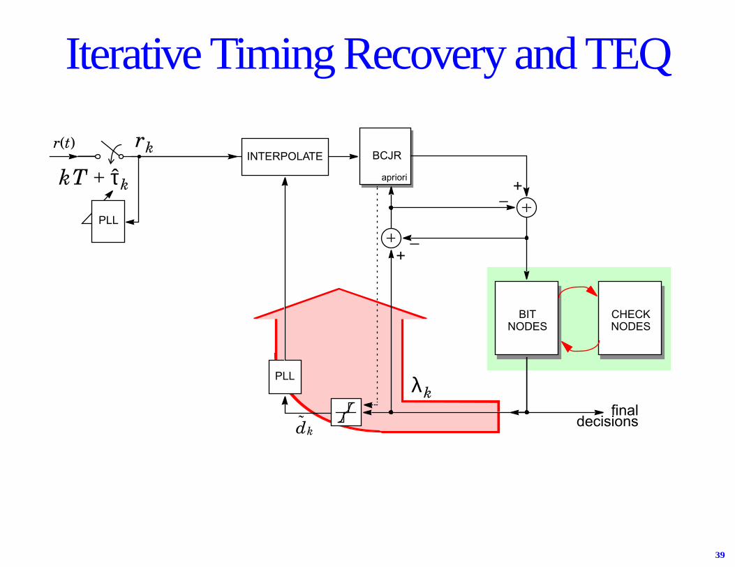
Iterative Timing Recovery and TEQ

BCJR

PLL

–+

–+

apriori

finaldecisions

PLL

r(t)

kT τk+

rk

dk

λk

INTERPOLATE

40

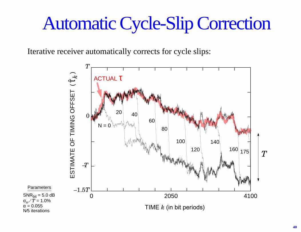
Iterative receiver automatically corrects for cycle slips:

Automatic Cycle-Slip Correction

σw ⁄T = 1.0%

Parameters

SNRbit = 5.0 dB 0 2050 4100– 1.5T

–T

0

T

TIME k (in bit periods)

ES

TIM

AT

E O

F T

IMIN

G O

FF

SE

T(

)ACTUAL τ

N = 0

20 4060

80

100

120140

160 175

τ k

α = 0.055N⁄5 iterations

T

41

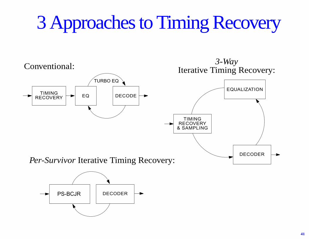
3 Approaches to Timing Recovery

TIMINGRECOVERY

& SAMPLING

EQUALIZATION

DECODER

TIMINGRECOVERY EQ DECODE

TURBO EQ

DECODER

Conventional: 3-Way

Per-Survivor Iterative Timing Recovery:

PS-BCJR

Iterative Timing Recovery:

42

Per-Survivor Processing

• A general framework for estimating Markov process with unknownparameters and independent noise

• Basic idea: Add a separate estimator to each survivor of Viterbi algorithm

• Has been applied to channel identification, adaptive sequence detection,carrier recovery

• Application to timing recovery [Kovintaveat et al., ISCAS 2003]:

❏ Start with traditional Viterbi algorithm on PR trellis❏ Run a separate PLL on each survivor, based on its decision history❏ Motivations:

➊ PLL is fully trained whenever correct path is chosen!➋ Can avoid decision delay altogether

[Raheli, Polydoros, Tzou 91-95]

43

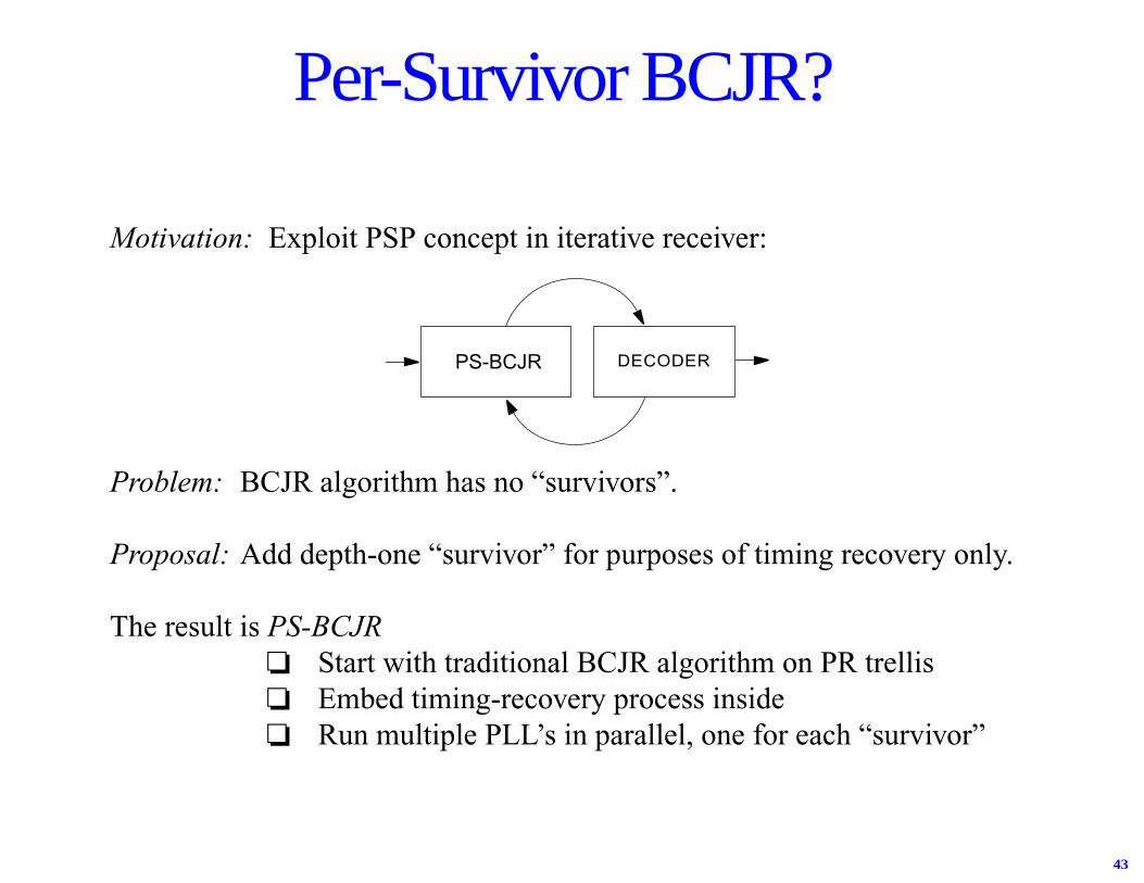
Motivation: Exploit PSP concept in iterative receiver:

Problem: BCJR algorithm has no “survivors”.

Proposal: Add depth-one “survivor” for purposes of timing recovery only.

The result is PS-BCJR❏ Start with traditional BCJR algorithm on PR trellis❏ Embed timing-recovery process inside❏ Run multiple PLL’s in parallel, one for each “survivor”

DECODERPS-BCJR

Per-Survivor BCJR?

44

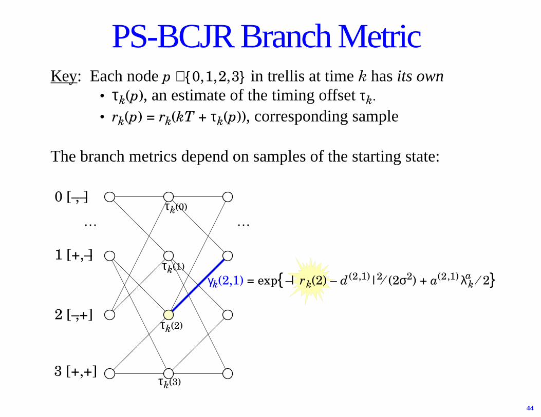
Key: Each node p ∈{0,1,2,3} in trellis at time k has its own• τk(p), an estimate of the timing offset τk.

• rk(p) = rk(kT + τk(p)), corresponding sample

The branch metrics depend on samples of the starting state:

… …

PS-BCJR Branch Metric

τk(0)

τk(1)

τk(2)

τk(3)

γk(2,1) = exp{–| rk(2) – d (2,1)|2⁄(2σ2) + a(2,1) λka ⁄2}

0 [–,–]

1 [+,–]

2 [–,+]

3 [+,+]

45

Per-Survivor BCJR: Forward Recursion

Associate with each node p ∈{0,1,2,3} at time k the following:• forward metric αk( p )• predecessor πk( p )• forward timing offset estimate τk( p )

αk+1(1) = 7 × 3 + 9 × 5 = 66

7

8

9

10

2

3

4

5

12

3

1

πk+1(1) = argmax0,2{7 × 3, 9 × 5} = 2τk+1(1) = τk( 2 ) + µ(rk(2)d(πk(2),2) – rk– 1(πk(2))d(2,1))

r(kT + τk(2)) r((k– 1)T + τk– 1(πk(2)))

Notation complicated, but idea is simple:update blue node timing using M&M PLL driven bythe samples & inputs corresponding to blue branches.

0

1

2

3

46

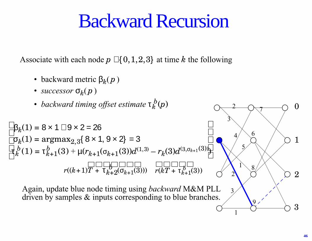
Backward Recursion

Associate with each node p ∈{0,1,2,3} at time k the following

• backward metric βk( p )• successor σk( p )

• backward timing offset estimate τkb(p)

βk(1) = 8 × 1 + 9 × 2 = 26

7

6

8

9

2

3

4

5

12

3

1

σk(1) = argmax2,3{8 × 1, 9 × 2} = 3τk

b (1) = τk+1b (3) + µ(rk+1(σk+1(3))d(1,3) – rk(3)d(3,σk+1(3)))

r((k+1)T + τk+2b (σk+1(3))) r(kT + τk+1

b (3))

Again, update blue node timing using backward M&M PLLdriven by samples & inputs corresponding to blue branches.

0

1

2

3

47

Compare Forward/Backward Timing

Backward timing estimates can exploit knowledge of forward estimates.

Option 1: Ignore forward estimates during backward pass.

Option 2: Average backward with forward estimate whenever they differ bymore than some threshold (say 0.1T) in absolute value.

48

PRECODER

mkakck 1

1 ⊕ D2

New Encoder

1 ⊕ D ⊕ D3 ⊕ D4

1 ⊕ D ⊕ D4 PU

NC

TU

RE π

S-RANDOMINTERLEAVER

(s = 16)

RATE-8 ⁄ 9LENGTH 4095

RSC ENCODER

49

TIMINGRECOVERY

& SAMPLING

EQUALIZATION

DECODER

TIMINGRECOVERY EQ DECODE

TURBO EQ

DECODER

Conventional:

Per-Survivor Iterative Timing Recovery:

PSP-BCJR

3-Way Iterative Timing Recovery:

Compare 3 Systems

Complexity = #IT × (PLL + BCJR + DEC)

Complexity = #IT × (8 × PLL + BCJR + DEC)

50

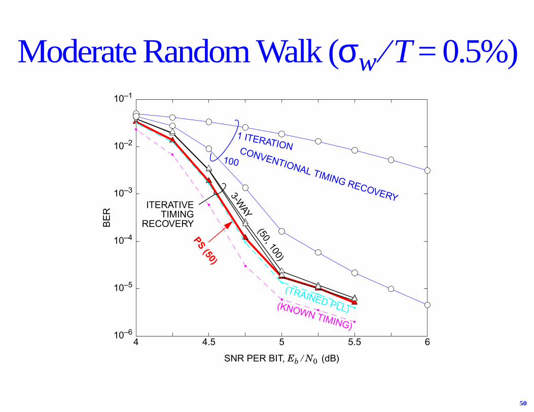
Moderate Random Walk (σw ⁄ T = 0.5%)

4 4.5 5 5.5 610–6

10–5

10–4

10–3

10–2

10–1

SNR PER BIT, Eb ⁄N0 (dB)

BE

R

CONVENTIONAL TIMING RECOVERY

1 ITERATION

100

(TRAINED PLL)

(50, 100)

3-WAY

PS (50)

(KNOWN TIMING)

ITERATIVETIMING

RECOVERY

51

4 4.5 5 5.5 6

SNR PER BIT, Eb ⁄N0 (dB)

10–6

10–5

10–4

10–3

10–2

10–1B

ER

Severe Random Walk (σw ⁄ T = 1%)

52

0 500 1000 1500 2000 2500 3000 3500 4000−0.5T

0

0.5T

T

1.5T

2T

2.5T

Timing Estimate

Tim

e (in

bit

perio

ds)

2

5

1

I−CTR (50)

Actual τ

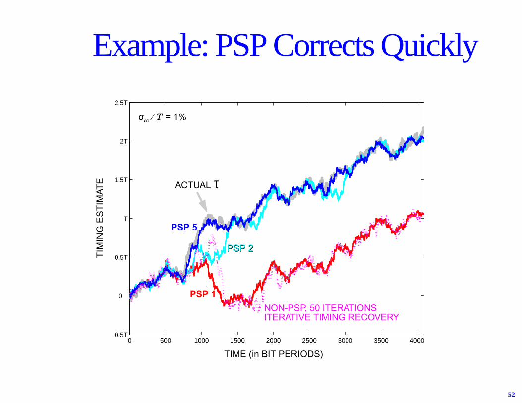
Example: PSP Corrects Quickly

ACTUAL τ

PSP 2PSP 2

PSP 5

PSP 1NON-PSP, 50 ITERATIONSITERATIVE TIMING RECOVERY

TIM

ING

ES

TIM

ATE

TIME (in BIT PERIODS)

σw ⁄T = 1%

53

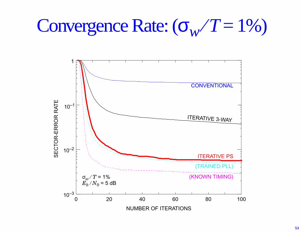
0 20 40 60 80 10010–3

10–2

1

NUMBER OF ITERATIONS

SE

CTO

R-E

RR

OR

RAT

E

10–1

σw ⁄T = 1%Eb ⁄N0 = 5 dB

(KNOWN TIMING)

(TRAINED PLL)

ITERATIVE PS

ITERATIVE 3-WAY

CONVENTIONAL

Convergence Rate: (σw ⁄ T = 1%)

54

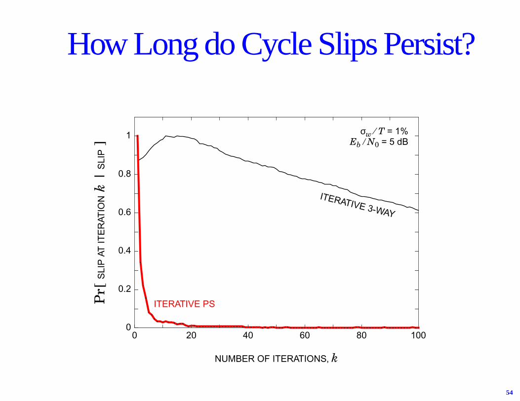
0 20 40 60 80 1000

0.2

0.4

0.6

0.8

1

Pr[

SLI

P A

T IT

ER

ATIO

Nk

|S

LIP

]

How Long do Cycle Slips Persist?

NUMBER OF ITERATIONS, k

ITERATIVE PS

ITERATIVE 3-WAY

σw ⁄T = 1%Eb ⁄N0 = 5 dB

55

❍ Powerful codes permit low SNR➢ conventional strategies fail➢ exploiting code is critical

❍ Problem is solvable

❍ We described two strategies for iterative timing recovery➢ Embed timing recovery inside turbo equalizer➢ Automatically corrects for cycle slips

❍ Challenges remaining➢ complexity➢ close gap to known timing

Summary