ITOMP: Incremental Trajectory Optimization for Real-time Replanning inDynamic Environments

Chonhyon Park and Jia Pan and Dinesh ManochaUniversity of North Carolina at Chapel Hill

http://gamma.cs.unc.edu/ITOMP/

Abstract

We present a novel optimization-based algorithm for motionplanning in dynamic environments. Our approach uses astochastic trajectory optimization framework to avoid colli-sions and satisfy smoothness and dynamics constraints. Ouralgorithm does not require a priori knowledge about globalmotion or trajectories of dynamic obstacles. Rather, we com-pute a conservative local bound on the position or trajectoryof each obstacle over a short time and use the bound to com-pute a collision-free trajectory for the robot in an incrementalmanner. Moreover, we interleave planning and execution ofthe robot in an adaptive manner to balance between the plan-ning horizon and responsiveness to obstacle. We highlight theperformance of our planner in a simulated dynamic environ-ment with the 7-DOF PR2 robot arm and dynamic obstacles.

1 IntroductionMotion planning is an important problem in many roboticsapplications, including autonomous navigation and taskplanning. Most of the earlier work on practical motion plan-ning algorithms is based on randomized algorithm (Kavrakiet al. 1996; Kuffner and LaValle 2000; LaValle 2006) andis mostly limited to static environments. However, robotsmust work reliably in dynamic environments with humansand other moving objects, e.g., when performing house-hold jobs like cleaning a room. Therefore, the robot needsto acquire the ability to safely navigate in the environ-ment and perform tasks in the presence of moving obsta-cles. In order to achieve this goal, many planning algorithmsfor dynamic environments have been proposed (van denBerg and Overmars 2005; Phillips and Likhachev 2011b;Hauser 2012). However, most of these methods assume thatthe future trajectories of dynamic obstacles are known a pri-ori during the planning computation. This assumption maynot hold in many real world applications. As a matter of fact,most moving objects’ motions are not precisely predictableor can only be approximated over a small or local time in-terval. Such uncertainty about moving objects makes it hardto plan a safe trajectory for the robot over a long horizon.

Another challenge in terms of planning in dynamic envi-ronments is that the planning algorithm must be responsive

Copyright c© 2012, Association for the Advancement of ArtificialIntelligence (www.aaai.org). All rights reserved.

to unpredictable situations, which requires real-time plan-ning capability in terms of computing or updating the trajec-tory. There is some recent work on accelerating high-DOFplaning algorithms, such as GPU parallelism (Pan, Lauter-bach, and Manocha 2010) or distributed systems (Devaurs,Simeon, and Cortes 2011). A real-time planner can improvethe responsiveness, but it may not provide an adequate so-lution for all situations. The reason is that there are difficultscenarios, e.g., narrow passages (LaValle 2006), which arehard for any planner in terms of real-time computation. Inthese cases, planning before task execution can lead to de-lays in the robot’s movement and decrease its safety. Onepossible solution for handling such scenarios is by interleav-ing planning with execution; the overall algorithm lands upcomputing partial or sub-optimal plans to avoid delays inits handling of moving obstacles (Petti and Fraichard 2005;Bekris and Kavraki 2007; Hauser 2012).

In order to overcome these challenges, we present an ef-ficient replanning framework based on optimization-basedapproaches. Our work is based on recent developmentsin optimization-based planning that can also handle dy-namic constraints efficiently (Kalakrishnan et al. 2011;Ratliff et al. 2009; Dragan, Ratliff, and Srinivasa 2011).In order to handle dynamic obstacles and perform realtimeplanning, our approach uses an incremental approach (IT-OMP). First, we estimate the trajectory of the moving obsta-cles over a short time horizon using simple estimation tech-niques. Next, we compute a conservative bound on the posi-tion of the moving obstacles based on the predicted motion.We then calculate a trajectory connecting robot’s initial andgoal configurations by solving an optimization problem thatavoids collisions with the obstacles and satisfies smooth-ness and torque constraints. In order to make the robot re-spond quickly to the dynamic environments, we interleaveplanning with task execution: that is, instead of solvingthe optimization problem completely, we assign a time bud-get for planning and interrupt the optimization solver whenthe time runs out. The computed trajectory may be sub-optimal, which means that 1) its objective cost may not beminimized; 2) the collision-free constraints or other addi-tional constraints may not be completely satisfied. The robotthen executes over the short time interval based on this sub-optimal path computation. We repeat these steps until therobot reaches the goal position. During each iterative step,

we update the conservative bound on the object’s positionand also account for any new objects that may have en-tered the robot’s workspace. The updated environment in-formation is incorporated into the optimization formulation,which uses the sub-optimal result from the last step as theinitial solution and tries to improve it incrementally withinthe given timing budget. We demonstrate the performanceof our replanning algorithm in the ROS simulation environ-ment where the PR2 robot tries to perform manipulation taskwith its 7-DOF robot arm.

The rest of the paper is organized as follows. We sur-vey related work on planning for dynamic environmentsand replanning in Section 2. Section 3 introduces the no-tation used in the paper and gives an overview of our ap-proach. We present our optimization-based replanning algo-rithm (ITOMP) in Section 4. We highlight its performanceon simulated dynamic environments in Section 5.

2 Related WorkIn this section, we give a brief overview of prior work onmotion planning in dynamic environments, realtime replan-ning and optimization-based planning.

Planning in Dynamic EnvironmentsMost of the approaches for motion planning in dynamic en-vironments assume that the trajectories of moving objectsare known a priori. Some of them model dynamic obstaclesas static obstacles with a short horizon and set a high costaround the obstacles. (Likhachev and Ferguson 2009). An-other common approach is to use velocity obstacles, whichare used to compute appropriate velocities to avoid col-lisions with dynamic obstacles (Fiorini and Shiller 1998;Wilkie, van den Berg, and Manocha 2009). However, thesemethods cannot give any guarantees on the optimality of theresulting trajectory.

Some of the planning methods handle the continuousstate space directly, e.g., RRT variants have been proposedfor planning in dynamic environments (Petti and Fraichard2005). For discrete state spaces, efficient planning algo-rithms for dynamic environment include variants of A* algo-rithm, which are based on classic heuristic searches (Phillipsand Likhachev 2011b; 2011a) and roadmap-based algo-rithms (van den Berg and Overmars 2005).

Most planning algorithms for dynamic envi-ronments (van den Berg and Overmars 2005;Phillips and Likhachev 2011b) assume that the inertialconstraints, such as acceleration and torque limit, arenegligible for the robot. Such an assumption implies thatthe robot can stop and accelerate instantaneously, whichmay not be the case for a physical robot.

Real-time ReplanningSince path planning can be computationally expensive, plan-ning before execution can lead to long delays during arobot’s movement. To handle such scenarios, real-time re-planning interleaves planning with execution so that therobot may decide to compute only partial or sub-optimalplans in order to avoid delays in the movement. Real-time

replanning methods differ in many aspects; one key differ-ence is the underlying planner used. Sample-based motionplanning algorithms such as RRT have been applied to real-time replanning for dynamic continuous systems (Hsu etal. 2002; Hauser 2012; Petti and Fraichard 2005). Thesemethods can handle high-dimensional configuration spacesbut usually cannot generate optimal solutions. A* variantssuch as D* (Koenig, Tovey, and Smirnov 2003) and anytimeA* (Likhachev et al. 2005) can efficiently perform replan-ning on discrete state spaces and provide optimal guarantees,but are mostly limited to low dimensional spaces. Most re-planning algorithms that interleave planning and executionuse fixed time steps (Petti and Fraichard 2005), althoughsome recent work (Hauser 2012) computes the interleavingtiming step in an adaptive manner so as to maintain a bal-ance between the safety, responsiveness, and completenessof the overall system.

Optimization-based Planning AlgorithmsThe most widely-used method of path optimization is theso-called ‘shortcut’ heuristic, which picks pairs of con-figurations along a collision-free path and invokes a localplanner to attempt to replace the intervening sub-path witha shorter one (Chen and Hwang 1998; Pan, Zhang, andManocha 2011). Another approach is based on Voronoidiagrams to compute collision-free paths (Garber and Lin2004). Other approaches are based on elastic bands or elas-tic strips, which use a combination of mass-spring systemsand gradient-based methods to compute minimum-energypaths (Brock and Khatib 2002; Quinlan and Khatib 1993).All these methods require a collision-free path as an ini-tial value to the optimization algorithm. Some recent ap-proaches, such as (Ratliff et al. 2009; Kalakrishnan et al.2011; Dragan, Ratliff, and Srinivasa 2011) directly encodethe collision-free constraints and use an optimization-basedsolver to transform a naive initial guess into a trajectory suit-able for robot execution.

3 OverviewIn this section, we introduce the notation used in the rest ofthe paper and give an overview of our approach.

We use the symbol C to represent the configuration spaceof a robot, including several C-obstacles and the free spaceCfree. Let the dimension of C be D. Each element in theconfiguration space, i.e., a configuration, is represented as adim-D vector q.

For a single planning step, suppose there areNs static ob-stacles and Nd dynamic obstacles in the environment. Thenumber of dynamic obstacles is changed between the stepsas the sensor introduces new obstacles and removes out ofrange obstacles and the information is kept for a planninginterval. We assume that these obstacles are all rigid bodies.For static obstacles, we denote them as Os

j , j = 1, ..., Ns.For dynamic obstacles, as their positions vary with time, wedenote them as Od

j (t), j = 1, ..., Nd. Osj and Od

j (t) corre-spond to the objects in the workspace, and we denote theircorresponding C-obstacles in the configuration space as COs

j

and COdj (t), respectively.

In the ideal case, we assume that we have completeknowledge about the motion and trajectory of dynamic ob-stacles, i.e., we know the functions Od

j (t) and COdj (t) ex-

actly. However, in real-world applications, we may onlyhave local estimates of the future movement of the dynamicobstacles. Moreover, the recent position and velocity of ob-stacles computed from the sensors may not be accurate dueto the sensing error. In order to guarantee safety of the plan-ning trajectory, we compute a conservative local bound onthe trajectories of dynamic obstacles during planning. Giventhe time instance tcur, the conservative bound for the mov-ing objectOd

j at time t > tcur bounds the shape correspond-ing to Od

j (t), and is computed as:

Od

j (t) = c(1 + es · t)Odj (t) (1)

where es is the maximum allowed sensing error. As thesensing error increases the conservative bound becomeslarger. When an obstacle has a constant velocity, it is guar-anteed that the conservative bound includes the obstacle dur-ing the time period corresponding to t > tcur with c = 1.However, if an obstacle changes its velocity, we have to usea larger value of c in our conservative bound, and it wouldbe valid for a shorter time interval. We can define the con-servative bound for a moving object Od

j during a given timeinterval I = [t0, t1] as follows:

Od

j (I) =⋃t∈IOd

j (t),∀t ∈ I, t > tcur. (2)

Similarly, we can define conservative bounds in the config-uration space, which are denoted as COd

j (t) and COd

j (I),respectively.

We treat motion planning in dynamic environments asan optimization problem in the configuration space, i.e.,we search for a smooth trajectory that minimizes the costcorresponding to collisions with moving objects and someadditional constraints, such as joint limit or accelerationlimit. Specifically, we consider trajectories correspondingto a fixed time duration T , discretized into N waypointsequally spaced in time. In other words, the discretized tra-jectory is composed of N configurations q1, ...,qN , whereqi is a trajectory waypoint at time i−1

N−1T . We can also rep-resent the trajectory as a vector Q ∈ RD·N :

Q = [qT1 ,q

T2 , ...,q

TN ]T . (3)

We assume that the start and goal configurations of the tra-jectory, i.e., qs and qg , are given, and are fixed during op-timization. Figure 1 illustrates the symbols used by ouroptimization-based planner.

Similarly to previous work (Ratliff et al. 2009; Kalakr-ishnan et al. 2011), our optimization problem is formalizedas:

minq1,...,qN

N∑i=1

c(qi) +1

2‖AQ‖2, (4)

where c(·) is an arbitrary state-dependent cost function,which can include obstacle costs for static and dynamicobjects, and additional constraints such as joint limit and

torque limit. That is, the cost function can be divided intothree parts:

c(q) = cs(q) + cd(q) + co(q), (5)

where cs(·) is the obstacle cost for static objects, cd(·) isthe obstacle cost for moving objects and co(·) is the cost foradditional constraints. As cd(·) changes along with time dueto movement of dynamic obstacles, we sometimes denote itas ctd(·) to show the dependency on time explicitly. A is amatrix that is used to represent the smoothness costs. Wechoose A such that ‖AQ‖2 represents the sum of squaredaccelerations along the trajectory. Specifically, A is of theform

A =

1 0 0 0 0 0−2 1 0 · · · 0 0 01 −2 1 0 0 0

.... . .

...0 0 0 1 −2 10 0 0 · · · 0 1 −20 0 0 0 0 1

⊗ID×D, (6)

where ⊗ denotes the Kronecker tensor product and ID×D isa square matrix of size D. It follows that Q = AQ, whereQ represents the second order derivative of the trajectory Q.

The solution to the optimization problem in Equation (4)corresponds to the optimal trajectory for the robot:

Q∗ = {q∗1 = qs,q∗2, ...,q

∗N−1,q

∗N = qg}. (7)

However, notice that Q∗ is guaranteed to be collision-freewith dynamic obstacles only during a short time horizon.Because we only have a rough estimation based on the ex-trapolation of the motion of the moving objects, rather thanan exact model of the moving objects’ motion, the cost func-tion ctd(·) is only valid within a short time interval. In orderto associate a period of validity with the result of our op-timization algorithm, we use Q∗I to represent the planningresult that is valid during the interval I = [t0, t1] ⊆ [0, T ].

In order to improve robot’s responsiveness and safety, weinterleave planning and execution threads, in which the robotexecutes a partial or suboptimal trajectory (based on a high-rate feedback controller) that is intermittently updated by thereplanning thread (at a lower rate) without interrupting theexecution. We assign a time budget ∆k to the k-th step ofreplanning, which is also the maximum allowed time for ex-ecution of the planning result from last step. We use a con-stant timing budget ∆t = ∆, but our approach can be easilyextended to use a dynamic timing budget that is adaptiveto replanning performance (Hauser 2012). The interleavingstrategy is subject to the constraint that the current trajectorybeing executed cannot be modified. Therefore, if the replan-ning result is sent to the robot for execution at time t, it isallowed to run for time ∆, and no portion of the computedtrajectory before t + ∆ may be modified. In other words,the planner should start planning from t + ∆. Due to lim-ited time budget, the planner may not be able to computean optimal solution of the optimization function shown inEquation (4) and the resulting trajectory may be, and usu-ally is, sub-optimal. Its cost may be greater than or equal to

dynamic obstacle COd

static obstacle COs

q1

qk

qN0

tT

C-Space at different time

I=

[t 0, t 1

]

COd([t0, t1])

Figure 1: Optimization-based motion planning for dynamic environments. We showhow the configuration space changes over time: each plane slice represents the con-figuration space at time t. In the environment, there are two C-obstacles: the staticobstacle COs and the dynamic obstacle COd. We need to plan a trajectory to avoidthese obstacles. The trajectory starts at time 0, stops at time T , and is represented bya set of way points q1, ..., qk , ..., qN . Supposing that the trajectory is to be executedby the robot during time interval I = [t0, t1], we only need to consider the conser-vative bound COd

([t0, t1]) for the dynamic obstacle during the time interval. TheC-obstacles shown in the red color correspond to the obstacles at time t ∈ I .

the cost of the optimal trajectory Q∗. i.e., f(Q∗I) ≤ f(Q∗I),

where we denote the resulting trajectory from the planner asQ∗I , and f(Q) =

∑Ni=1 c(qi) + 1

2‖AQ‖2.

4 ITOMP AlgorithmIn this section, we present our ITOMP algorithm for plan-ning in dynamic environments, i.e., how to solve the opti-mization problem corresponding to Equation (4). We firstintroduce the cost metric for static obstacles and dynamicobstacles. Next, we present our incremental optimizationalgorithm.

Obstacle CostsSimilarly to prior work (Kalakrishnan et al. 2011; Ratliffet al. 2009), we model the cost of static obstacles usingsigned Euclidean Distance Transform (EDT). We start witha boolean voxel representation of the static environment, ob-tained either from a laser scanner or from a triangle meshmodel. Next, the signed EDT d(x) for a 3D point x iscomputed throughout the voxel map. This provides infor-mation about the distance from x to the boundary of theclosest static obstacle, which is negative, zero or positivewhen x is inside, on the boundary or outside the obstacles,respectively. One advantage of EDT is that it can encodethe discretized information about penetration depth, contact

and proximity in a uniform manner and can make the op-timization algorithm more robust. After the signed EDT iscomputed, the planning algorithm can efficiently check forcollisions by table lookup in the voxel map. In order to com-pute the obstacle cost, we approximate the robot shape B bya set of overlapping spheres b ∈ B. The static obstacle costis as follows:

cs(qi) =∑b∈B

max(ε+ rb − d(xb), 0)‖xb‖, (8)

where rb is the radius of one sphere b, xb is the 3D pointof sphere b computed from the kinematic model of the robotin configuration qi, and ε is a small safety margin betweenrobot and the obstacles. The speed of sphere b, ‖xb‖, ismultiplied to penalize the robot when it tries to traverse ahigh-cost region quickly. The static obstacle cost is zerowhen all the sphere are at least ε distance away from theclosest obstacle.

EDT computation is efficient for static obstacles but can-not be applied to dynamic obstacles, though a GPU-basedparallel EDT computation algorithm could be used (Sud,Otaduy, and Manocha 2004). The reason is that the move-ment of dynamic obstacles implies that EDT needs to be re-computed during each time step and it is hard to performsuch computation in real-time on current CPUs. Instead, weperform geometric collision detection between the robot andmoving obstacles and use the collision result to formalizethe dynamic obstacle cost. Given a configuration qi on thetrajectory and the geometric representation of moving obsta-clesOs

j at the corresponding time (i.e., i−1N−1T ), the obstacle

cost corresponding to configuration qi is given as:

cd(qi) =∑j

is collide(Os

j(i− 1

N − 1T ),B), (9)

where is collide(·, ·) returns one when there is a colli-sion and zero otherwise. The is collide function can beperformed efficiently using object-space collision detectionalgorithms, such as (Gottschalk, Lin, and Manocha 1996).This obstacle cost function is only used during a short or lo-cal time interval, i.e. from replanning’s start time t to its endtime t + ∆, since the predicted positions of dynamic obsta-cles can have high uncertainty during a long time horizon.

Dynamic Environment and ReplanningITOMP makes no assumption about the global motion or tra-jectory of each moving obstacle. Instead, we predict the fu-ture position and the velocity of moving obstacles based ontheir recent positions, which are generated from noisy sen-sors. This prediction and maximum error bound are used tocompute a conservative bound on the moving obstacles dur-ing the local time interval. Therefore, the planning result isguaranteed to be safe only during a short time period. In or-der to offer quick response during unpredictable cases (e.g.,the trajectory prediction about some of the objects is not cor-rect or new moving obstacles enter the robot’s workspace),the robot must sense the environment frequently and theplanner needs to be interrupted to update the description ofthe environment.

PLANNING PLANNING PLANNING PLANNING

EXECUTION

EXEC.

EXECUTION

EXECUTION

step 0 step 1 step 2 step n− 1 step n

t0 t1 t2 tn−1 tn tn+1t3

∆0 ∆1 ∆2 ∆n−1 ∆n tf

goal

time

predict model in [t1, t2] predict model in [t2, t3] predict model in [t3, t4] predict model in [tn,∞]

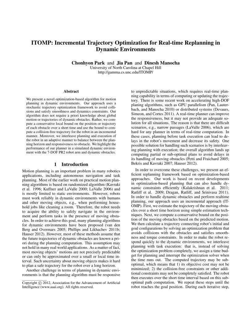
Figure 3: Interleaving of planning and execution. The planner starts at time t0. During the first planning time budget [t0, t1], it plans a safe trajectory for the first execution interval[t1, t2], which is also the next planning interval. In order to compute the safe trajectory, the planner needs to compute a conservative bound for each moving obstacle during [t1, t2].The planner is interrupted at time t1 and the ITOMP scheduling module notifies the controller to start execution. Meanwhile, the planner starts the planning computation for the nextinterval [t2, t3], after updating the bounds on the trajectory of the moving obstacles. Such interleaving of planning and execution is repeated until the robot reaches the goal position.In this example, n interleaving steps are used, and the time budget allocated to each step is ∆i, which can be fixed or changed adaptively. Notice that if the robot is currently is anopen space, the planner may compute an optimal solution before the time budget runs out (e.g., during [t2, t3]).

Ready

Monitor

Finish

Goal Motion Planner

RobotController

Sensor

Setting

Scheduling Module

Data

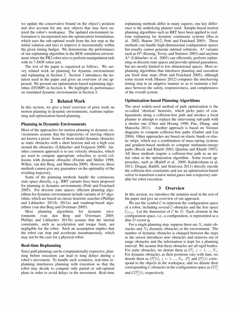
Figure 2: The overall pipeline of ITOMP: the scheduling module runs the main algo-rithm. It gets input from the user and interleaves the planning and execution threads.The Motion Planner module computes the trajectory for the robot and the Robot Con-troller module is used to execute the trajectory. The planner also receives updatedenvironment information frequently from sensors.

In order to handle uncertainty from moving obstacles andprovide high responsiveness, ITOMP interleaves planningand execution of the robot. As illustrated in Figure 2, IT-OMP consists of several parts: the scheduling module, themotion planner, the robot controller and the data-collectingsensor. The scheduling module gets the goal information asinput and controls the other modules. When a new goal po-sition is set, the scheduling module sends a new trajectorycomputation request to the motion planner. When the mo-tion planner computes a new trajectory that is safe within ashort horizon, the scheduling module notifies the robot con-troller to execute the trajectory. Meanwhile, it also sends anew request to the motion planner to compute a safe trajec-tory for the next execution interval. The planner also needsto incorporate the updated environment description from thesensor data. Since the motion planner runs in a separatethread, the scheduling module does not need to wait for theplanner to terminate. Instead, it checks whether the robotreaches the goal, updates the dynamic environment descrip-tion, and checks whether the planner has computed a newtrajectory.

The details about the interleaved planning and executionmethod are shown in Figure 3. The i-th time step of short-horizon planning has a time budget ∆i = ti+1− ti, which isalso the time budget for the current step of execution. Dur-ing the i-th time step, the planner tries to generate a trajec-tory by solving the optimization problem in Equation 4. Thetrajectory should be valid during the next step of execution,i.e., during the time interval [ti+1, ti+2].

Due to the limited time budget, the planner may only beable to compute a sub-optimal solution before it is inter-rupted. The sub-optimal solution may not be collision-freeor may violate some other constraints during the next execu-tion interval [ti+1, ti+2]. To handle such cases, we use twotechniques. First, we assign higher weights to the obstaclecosts related to the trajectory waypoints during the interval[ti+1, ti+2], which biases the optimization solver to reducethe cost during the execution interval. If the optimizationresult is not valid during the execution interval, ITOMP’sscheduling module chooses not to execute during the follow-ing execution interval. This approach keeps the planner fromviolating hard constraints(e.g. torque, end effector orienta-tion, etc.) and allocates more time to the planner to improvethe result. If the optimization result is valid but not optimal,i.e., the cost is not minimized during time interval [ti+2,∞],the planner can also improve it incrementally during follow-ing time intervals. The time budget for each step of short-horizon planning can be changed adaptively according to thequality of the resulting trajectory, which tries to balance therobot’s responsiveness and safety (Hauser 2012).

Notice that usually the optimization can converge to lo-cal optima quickly because during the i-th step planning weuse the result of (i − 1)-th step as the initial value. On theother hand, the optimization algorithm tends to compute asub-optimal solution when the robot is near a region withmultiple minima in the configuration space or a narrow pas-sage.

5 ResultsIn this section, we highlight the performance of our plan-ning algorithm in dynamic environments. We have imple-mented our algorithm in a simulator that uses the geometricand kinematic model of Willow Garage’s PR2 robot in theROS environment. All the experiments are performed on aPC equipped with an Intel i7-2600 8-core CPU 3.4GHz with8GB of memory. Our experiments are based on the accuracyof the PR2 robot’s LIDAR sensor (i.e. 30mm), and the plan-ning routines obtain information about dynamic obstacles(positions and velocities) every 200 ms.

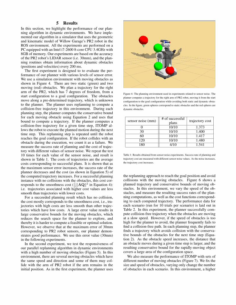
The first experiment is designed to to evaluate the per-formance of our planner with various levels of sensor error.We use a simulation environment with moving obstacles asshown in Figure 4. There are two static (green) and twomoving (red) obstacles. We plan a trajectory for the rightarm of the PR2, which has 7 degrees of freedom, from astart configuration to a goal configuration. The obstaclesmove along a pre-determined trajectory, which is unknownto the planner. The planner uses replanning to compute acollision-free trajectory in this environment. During eachplanning step, the planner computes the conservative boundfor each moving obstacle using Equation 2 and uses thatbound to compute a trajectory. If the planner computes acollision-free trajectory for a given time step, ITOMP al-lows the robot to execute the planned motion during the nexttime step. This replanning step is repeated until the robotreaches the goal configuration. If the robot collides with anobstacle during the execution, we count it as a failure. Wemeasure the success rate of planning and the cost of trajec-tory with different values of sensor noise. We repeat the test10 times for each value of the sensor noise, and result isshown in Table 1. The costs of trajectories are the averagecosts corresponding to successful plans. It is shown that asthe maximum sensor error increases, the success rate of theplanner decreases and the cost (as shown in Equation 5) ofthe computed trajectory increases. For a successful planninginstance with no collisions with the obstacles, this cost cor-responds to the smoothness cost ( 1

2‖AQ‖2 in Equation 4):i.e. trajectories associated with higher cost values are lesssmooth than trajectories with lower costs.

For a succeeded planning result which has no collision,the cost mostly corresponds to the smoothness cost, i.e., tra-jectories with high costs are less smooth than other trajec-tories which have low costs. A large error value results inlarge conservative bounds for the moving obstacles, whichreduces the search space for the planner to explore, andthereby it is harder to compute a feasible or optimal solution.However, we observe that at the maximum error of 30mmcorresponding to PR2 robot sensors, our planner demon-strates good performance. We use this error value (30mm)in the following experiments.

In the second experiment, we test the responsiveness ofour parallel replanning algorithm in dynamic environmentswith a high number of moving obstacles (Figure 5). In thisenvironment, there are several moving obstacles which havethe same speed and direction and some of them may col-lide with the arm of PR2 robot if the arm remains in theinitial position. As in the first experiment, the planner uses

Figure 4: The planning environment used in experiments related to sensor noise. Theplanner computes a trajectory for the right arm of PR2 robot, moving it from the startconfiguration to the goal configuration while avoiding both static and dynamic obsta-cles. In the figure, green spheres correspond to static obstacles and the red spheres aredynamic obstacles.

sensor noise (mm) # of successfulplans trajectory cost

0 10/10 1.37330 10/10 1.40060 10/10 1.417

120 10/10 1.480180 4/10 1.541

Table 1: Results obtained from sensor noise experiments. Success rate of planning andtrajectory cost are measured with different sensor noise values. As the noise increases,the trajectory cost increases.

the replanning approach to reach the goal position and avoidcollisions with the moving obstacles. Figure 6 shows aplanned trajectory and conservative bounds of moving ob-stacles. In this environment, we vary the speed of the ob-stacles, and measure the resulting success rates of the plan-ning computations, as well as the cost functions correspond-ing to each computed trajectory. The performance data foreach scenario (run for 10 trials per scenario) is laid out inTable 2. In this experiment, the planner successfully com-pute collision-free trajectory when the obstacles are movingat a slow speed. However, if the speed of obstacles is toohigh for the planner to avoid, the planner frequently fails tofind a collision-free path. In each planning step, the plannerfinds a trajectory which avoids collision with the conserva-tive bounds of the obstacles for the next time step (Equa-tion 2). As the obstacle speed increases, the distance thatan obstacle moves during a given time step is larger, and theresulting conservative bound for the rapidly-moving objectcovers a large area of the configuration space.

We also measure the performance of ITOMP with sets ofdifferent number of moving obstacles (Figure 7). We fix thesize and speed of obstacles, varying only change the numberof obstacles in each scenario. In this environment, a higher

(a) (b) (c) (d)

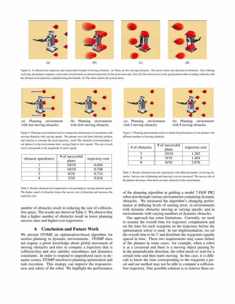
Figure 6: A collision-free trajectory and conservative bounds of moving obstacles. (a) There are five moving obstacles. The arrows shows the direction of obstacles. (b)(c) Duringeach step, the planner computes conservative local bounds on obstacle trajectory for the given time step. (b)(c)(d) The robot moves to the goal position while avoiding collisions withthe obstacle local trajectory computed using the bounds. (d) The robot reaches the goal position.

(a) Planning environmentwith fast-moving obstacles

(b) Planning environmentwith slow-moving obstacles

Figure 5: Planning environments used to evaluate the performance of our planner withmoving obstacles with varying speeds. The planner uses the latest obstacle positionand velocity to estimate the local trajectory. (a)(b) The obstacles (corresponding tored spheres) in the environment have varying (high or low) speeds. The size of eacharrow corresponds to the magnitude of each’s speed.

obstacle speed(m/s) # of successfulplans trajectory cost

1 10/10 0.6942 10/10 0.7483 8/10 0.7144 3/10 0.816

Table 2: Results obtained from experiments corresponding to varying obstacle speeds.The higher speed of obstacles lowers the success rate of planning and increases thetrajectory cost.

number of obstacles result in reducing the size of collision-free space. The results are shown in Table 3. We observe thatthat a higher number of obstacles result in lower planningsuccess rates and higher-cost trajectories.

6 Conclusion and Future WorkWe present ITOMP, an optimization-based algorithm formotion planning in dynamic environments. ITOMP doesnot require a priori knowledge about global movement ofmoving obstacles and tries to compute a trajectory that iscollision-free and also satisfies smoothness and dynamicsconstraints. In order to respond to unpredicted cases in dy-namic scenes, ITOMP interleaves planning optimization andtask execution. This strategy can improve the responsive-ness and safety of the robot. We highlight the performance

(a) Planning environmentwith 3 moving obstacles

(b) Planning environmentwith 8 moving obstacles

Figure 7: Planning environments used to evaluate the performance of our planner withdifferent numbers of moving obstacles.

# of obstacles # of successfulplans trajectory cost

3 10/10 1.3825 9/10 1.4048 6/10 2.876

Table 3: Results obtained from the experiments with different number of moving ob-stacles. Success rate of planning and trajectory cost are measured. The success rate ofthe planner decreases when there are more obstacles in the environment.

of the planning algorithm at guiding a model 7-DOF PR2robot arm through various environments containing dynamicobstacles. We measured the algorithm’s changing perfor-mance at differing levels of sensing error; in environmentswith dynamic obstacles moving at varying speeds; and inenvironments with varying numbers of dynamic obstacles.

Our approach has some limitations. Currently, we needto assume the overall time for trajectory computation andset the time for each waypoint on the trajectory before theoptimization solver is used. In our implementation, we setthe overall time to be T and distribute the waypoints equallyspaced in time. These two requirements may cause failureof the planner in some cases: for example, when a robotis at a crossroad and there is a moving object passing byin the perpendicular direction, the robot needs to wait for acertain time and then starts moving. In this case, it is diffi-cult to know the time corresponding to the waypoint a pri-ori and our method may not be able to compute a collision-free trajectory. One possible solution is to remove these as-

sumptions and solve the trajectory using dynamic program-ming similar to (Vernaza and Lee 2011). However, we needan incremental optimization solver to use interleaved plan-ning and execution to obtain high responsiveness and safety.Recently, we have developed a parallel version of ITOMPfor multi-core CPUs and many-core GPUs (Park, Pan, andManocha 2012). In particular, we show that by exploitingcommodity parallelism, we can considerably improve the re-sponsiveness and performance of the planner.

7 AcknowledgmentsThis work was supported by ARO Contract W911NF-10-1-0506, NSF awards 1000579 and 1117127, and WillowGarage.

ReferencesBekris, K., and Kavraki, L. 2007. Greedy but safe re-planning under kinodynamic constraints. In Robotics andAutomation, 2007 IEEE International Conference on, 704–710.Brock, O., and Khatib, O. 2002. Elastic strips: A frameworkfor motion generation in human environments. InternationalJournal of Robotics Research 21(12):1031–1052.Chen, P., and Hwang, Y. 1998. Sandros: a dynamic graphsearch algorithm for motion planning. IEEE Transactionson Robotics and Automation 14(3):390–403.Devaurs, D.; Simeon, T.; and Cortes, J. 2011. Paralleliz-ing rrt on distributed-memory architectures. In Proceedingsof IEEE International Conference on Robotics and Automa-tion, 2261 –2266.Dragan, A.; Ratliff, N.; and Srinivasa, S. 2011. Manipu-lation planning with goal sets using constrained trajectoryoptimization. In Proceedings of IEEE International Confer-ence on Robotics and Automation, 4582–4588.Fiorini, P., and Shiller, Z. 1998. Motion planning in dy-namic environments using velocity obstacles. InternationalJournal of Robotics Research 17(7):760–772.Garber, M., and Lin, M. C. 2004. Constraint-based mo-tion planning using voronoi diagrams. In Algorithmic Foun-dations of Robotics V, volume 7 of Springer Tracts in Ad-vanced Robotics. 541–558.Gottschalk, S.; Lin, M. C.; and Manocha, D. 1996. Obbtree:a hierarchical structure for rapid interference detection. InSIGGRAPH, 171–180.Hauser, K. 2012. On responsiveness, safety, and com-pleteness in real-time motion planning. Autonomous Robots32(1):35–48.Hsu, D.; Kindel, R.; Latombe, J.-C.; and Rock, S. 2002.Randomized kinodynamic motion planning with movingobstacles. International Journal of Robotics Research21(3):233–255.Kalakrishnan, M.; Chitta, S.; Theodorou, E.; Pastor, P.; andSchaal, S. 2011. STOMP: Stochastic trajectory optimizationfor motion planning. In Proceedings of IEEE InternationalConference on Robotics and Automation, 4569–4574.

Kavraki, L.; Svestka, P.; Latombe, J. C.; and Overmars, M.1996. Probabilistic roadmaps for path planning in high-dimensional configuration spaces. IEEE Transactions onRobotics and Automation 12(4):566–580.Koenig, S.; Tovey, C.; and Smirnov, Y. 2003. Performancebounds for planning in unknown terrain. Artificial Intelli-gence 147(1-2):253–279.Kuffner, J., and LaValle, S. 2000. RRT-connect: An effi-cient approach to single-query path planning. In Proceed-ings of IEEE International Conference on Robotics and Au-tomation, 995 – 1001.LaValle, S. M. 2006. Planning Algorithms. CambridgeUniversity Press.Likhachev, M., and Ferguson, D. 2009. Planning long dy-namically feasible maneuvers for autonomous vehicles. In-ternational Journal of Robotics Research 28(8):933–945.Likhachev, M.; Ferguson, D.; Gordon, G.; Stentz, A.; andThrun, S. 2005. Anytime dynamic A*: An anytime, replan-ning algorithm. In Proceedings of the International Confer-ence on Automated Planning and Scheduling.Pan, J.; Lauterbach, C.; and Manocha, D. 2010. g-Planner: Real-time motion planning and global navigationusing GPUs. In Proceedings of AAAI Conference on Artifi-cial Intelligence.Pan, J.; Zhang, L.; and Manocha, D. 2011. Collision-freeand curvature-continuous path smoothing in cluttered envi-ronments. In Proceedings of Robotics: Science and Systems.Park, C.; Pan, J.; and Manocha, D. 2012. Real-timeoptimization-based planning in dynamic environments usingGPUs. Technical report, Department of Computer Science,University of North Carolina at Chapel Hill.Petti, S., and Fraichard, T. 2005. Safe motion planningin dynamic environments. In Proceedings of IEEE/RSJ In-ternational Conference on Intelligent Robots and Systems,2210–2215.Phillips, M., and Likhachev, M. 2011a. Planning in do-mains with cost function dependent actions. In Proceedingsof AAAI Conference on Artificial Intelligence.Phillips, M., and Likhachev, M. 2011b. SIPP: Safe intervalpath planning for dynamic environments. In Proceedingsof IEEE International Conference on Robotics and Automa-tion, 5628–5635.Quinlan, S., and Khatib, O. 1993. Elastic bands: connectingpath planning and control. In Proceedings of IEEE Inter-national Conference on Robotics and Automation, 802–807vol.2.Ratliff, N.; Zucker, M.; Bagnell, J. A. D.; and Srinivasa,S. 2009. CHOMP: Gradient optimization techniques forefficient motion planning. In Proceedings of InternationalConference on Robotics and Automation, 489–494.Sud, A.; Otaduy, M. A.; and Manocha, D. 2004. DiFi:Fast 3d distance field computation using graphics hardware.Computer Graphics Forum 23(3):557–566.van den Berg, J., and Overmars, M. 2005. Roadmap-basedmotion planning in dynamic environments. IEEE Transac-tions on Robotics 21(5):885–897.

Vernaza, P., and Lee, D. D. 2011. Learning dimensionaldescent for optimal motion planning in high-dimensionalspaces. In Proceedings of AAAI Conference on ArtificialIntelligence.Wilkie, D.; van den Berg, J. P.; and Manocha, D. 2009.Generalized velocity obstacles. In Proceedings of IEEE/RSJInternational Conference on Intelligent Robots and Systems,5573–5578.