Linear algebra deals with systems of equations that are related linearly. It has many applications in multidimensional vector calculus, and related fields.
Systems of Linear Equations : a group of equations that share variables. The variables can be functions of other variables, as long as they are linear (simple polynomials).
Example: 5x + 2y –3z = 82x + z = 62z – y = 1
All three equations involve the variable x, y, and z with different coefficients.
Solving Systems of Linear Equations: determining numerical (or functional) values of the variables that satisfy ALL of the equations. There are two basic methods:
1. Elimination method: this is done by finding simple functional relationships between the variables, and substituting the functional forms:
Example: 5x + 2y –3z = 82x + z = 6 x = (6–z)/22z – y = 1 y = 2z–1
Plugging in the two functions of z into the first equation:
5x + 2y –3z = 5((6–z)/2 + 2(2z–1) – 3z = 8 15 – 5z/2 + 4z – 2 – 3z = 8 13 – 3z/2 = 8 z = 10/3 y = 17/3, and x = 4/3
The example shown above is very simple, and is not very general, since it is not always possible to write the simple functions. Instead, we must use some rules of algebra to come up with a better method.
2. Addition method: adding Linear Equations: If Eq1 and Eq2 are two linear equations that comprise a system of linear equations, then
mEq1 ± nEq2 (where n and m are real number multiples) is also a member of the system of linear equations. By doing this type of addition, one can eliminate variables from the equations to get a set of new equations, each consisting of only one of the variables.
Example: x + y – 3z = 2 5x + 5y – 15z = 10–5x – y + 5z = –3 x – 2y + 2z = 4
By adding 5 times equation 1 to equation 2, we get: 5x + 5y – 15z = 10
Adding equation 1 to equation 2 gives: x + y – 3z = 2 +(–5 x – y + 5 z = –3) –4x + 2z = –1
We can continue this until we have manageable equations that can be used as they were in the original problem, or we can go further and achieve the goal of getting three equations, each of 1 variable.
Note - Our examples contained 3 equations and 3 unknowns. Solutions to sets like that are said to be simple, since only one unique set of values for x, y, and z work. If there are MORE variables than equations, the best we can hope for is a set of solutions that rely on one or more of the variables remaining a variable. The "known" values will be expressed as functions of the "unknown" variables. This is the case with parallel lines.
Matrices
Matrix is an array of numbers in an n by m grid corresponding to a system of linear equations. Each cell in the grid corresponds to an element in one of the equations:
The variables, xj, are multiplied by the coefficients, akj, where k is the counting number for the equation and j is the counting number for the variable.
A matrix representation of the series of equations is (for simplicity we have shrunk it down to 3 equations):
(a11 a12 a13
a21 a22 a23
a31 a31 a33)( x1
x2
x3)=(b1
b2
b3) ⇔ Ax=b
Each row represents one of the equations, and each column (except the last) represents the coefficient of one of the variables. The last column contains the unique solutions to the equations represented in the rows of the matrix. We will come back to the systems of linear equations again later: first we have to learn a whole bunch of stuff about matrices.
Matrix Elements and Indices: Elements of a matrix are specified by a pair of indices: aij the first index is the number of the row, the second index of the column in the matrix
Dimension of Matrix: A matrix is said to be of m x n dimension if it has m rows and n columns
Vectors as Row Matrices: Vectors could be thought of as special cases of matrices where m or n=1. If m=1 we have a row vector:
x=(x1 , x2 , x3 )=x1 i+ x2 j+ x3 k(in the last equality written in some basis of i, j, k vectors).
If n = 1, like in the matrix form of three linear equations above, we have a column vector:
(x1
x2
x3)
Transpose of a Matrix or a Vector: Transpose turns a row into a column and vice versa. A transpose of a row vector x, for example would be a column vector xT, such that:
x=(x1 x2 x3 ) xT=(x1
x2
x3)
Row and column vectors are to some extent equivalent, however, each form serves a particular purpose in vector-matrix operations.
For a matrix, a transpose of m n matrix is an n m matrix, where rows became columns and columns rows:
A=(a11a21
a12a22
a13a23 ) AT=(a11
a12
a13
a21
a22
a23)
In matrix elements we write:aijT =a ji
In other words, the indices switched: row is column and column is row. Note that(AT)T = A
Symmetric matrices: symmetric matrix equals its transpose, i.e.AT = A
Oraij = aji
Note that only a square matrix (m = n) can be symmetric !
Example:
(1 44 3 ) ( 7 1+i 2 i
1+i 2 1−i2 i 1−i −5 )
Hermitian conjugate and Hermitian matrices: Hermitian conjugate A† to a matrix A is the transpose and complex conjugate (complex conjugate means that all elements become their complex conjugates):
Hermitian matrix is equal to its Hermitian conjugate:A = A†
A= ( 1 i−i −1 ) = (1
¿ (−i )¿
i¿ (−1 )¿ ) is Hermitian.
Note that any REAL symmetric matrix is also Hermitian (because the complex conjugate of a real number is the number itself), but a symmetric COMPLEX matrix is NOT:
(1 44 3 ) is Hermitian,
( 7 1+i 2 i1+i 2 1− i2 i 1−i −5 )
is not Hermitian.
Identity or Unity Matrix: To insure that matrices follow normal rules of algebra, there must be a matrix equivalent of the multiplicative identity, i.e. the number 1. For square matrices (i.e. those with the same number of rows as columns), for example for 3x3 matrices the identity or unity matrix is:
{ I=I=(1 0 00 1 00 0 1 )¿
This matrix falls into a special class of matrices known as Diagonal Matrices, since only elements along the diagonal are present. We will see later that a diagonal matrix has special properties.
Zero of Null matrix: A matrix whose elements are all zero
Other "special" matrices include "upper triangular matrices" where only the diagonal and elements above the diagonal appear, and "block diagonal" where the matrix looks like it is made of several smaller matrices, all strung together along the diagonal.
Matrix Algebra
Matrix Addition: Two matrices of the same dimension may be added. This is very similar to vector addition, i.e.:
(ad be
cf )+(g
jhk
il ) =(a+g
d+ jb+he+k
c+if + l )
note that the matrices have to be the same size (e.g. in this case 2 x 3)
Scalar Multiplication of a Matrix: A matrix may be multiplied by a number, resulting in a matrix whose elements are each scaled by the multiple, i.e.:
Multiplication of Matrices: The matrix multiplication is defined as a scalar product of the row of the first matrix with the column of the second matrix. As you recall, the scalar (dot) product of two vectors is the sum of product of all the elements. For this to work the two matrices must share the "inner dimension". I.e.
Amxn • Bnxp = CmxpThe dimension of the resultant matrix is always the row dimension of the first matrix and the column dimension of the second. This is the origin of the term "inner product".
In matrix multiplication, the scalar product of the i-th row of the first matrix with the j-th column of the second matrix gives the element in the i-th row and j-th column of the resulting matrix:
A ¿B=C
(a11
a21
a12
a22
a13
a23 ) ¿(b11b21b31
b12b22b32
)=( a11 b11+a12b21+a13 b31
first row and first columna11 b12+a12 b22+a13 b32
first row and second column
a21 b11+a22b21+a23 b31second row and first column
a21b12+a22b22+a23b32second row and second column
)=(c11 c12
c21 c22 )In the element notation, the multiplication of two matrices is written as:
c ik=∑j=1
n
a ij b jk, i = 1, 2 , …m; k = 1, 2, …, p
Note: Even though the "dot product" described in the vector algebra section of the course was invariant under commutation (i.e. A•B = B•A), the inner product of matrices does not share this property. In other words, multiplication of matrices is NOT commutative:
A•B B•AIt can be easily seen from the above examples, that for general rectangular matrices (m n) it cannot work:
(a11
a21
a12
a22
a13
a23 ) ¿ (b11 b12 b13
b21 b22 b23
b31 b32 b23)
=(a11 b11+a12b21+a13b31
a21b11+a22 b21+a23 b31
a11 b12+a12 b22+a13 b32
a21b12+a22b22+a23b32
a11 b13+a12b23+a13 b33
a21b13+a22b23+a23b33 ) (b11 b12 b13
b21 b22 b23
b31 b32 b23)¿(a
11a21
a12
a22
a13
a23 ) =Does NOT exist!
Even for square matrices, A•B and B•A is generally not the same thing:
(1 22 2 )¿(2 0
3 1 )=( 8 210 2 ) ≠ (2 0
3 1 ) ¿ (1 22 2 )=(2 2
5 8 )Transpose of the product of two matrices: the transpose of the product is the product of transposes of the individual matrices, but in reverse order:
(A • B)T = BT • AT
It is clear that the order must be reversed from the above discussion, since inner dimensions have to match.
Initially, when we introduced the matrix, we referred to the elements in matrix as the coefficients of the variables in the system of linear equations. We will improve upon that definition.
Operator: This is a matrix that acts as a function (or mapping) of a vector. When the operator operates on the vector, the result is also a vector!
Let us consider the system of equations:Eq 1: a11x + a12y + a13z = b1Eq 2: a21x + a22y + a23z = b2Eq 3: a31x + a32y + a33z = b3
In matrix notation, we wrote this as:A x=b
(a11 a12 a13
a21 a22 a23
a31 a32 a33)¿ ( x
yz )=(b1
b2
b3)
The “hat” symbol above the matrix denotes that it is an operator (usually it is omitted). The matrix here symbolizes some operation on the “input” vector (x) which yields some other, “output” vector b.
Examples: 1. rotation of a vector by an angle :
(ax'
a y' )=(cos (θ ) −sin (θ )
sin (θ ) cos (θ ) )(ax
a y) ax
' =ax cos (θ )−a y sin (θ )a y
' =ax sin (θ )+ay cos (θ )
2. mirror image of a vector with respect to xy plane:
(bx
b y
bz)=(1 0 0
0 1 00 0 −1 )(
ax
a y
az) bx = ax
b y = a ybz = −az
Operations on vectors can therefore be done by multiplying the vectors by operator matrices. Because vectors are only special cases of matrices, the rules of multiplication are the same. To operate on a vector with the matrix operator, the matrix has to have the same number of columns as the vector has rows. The result is a vector with the same number of rows as the matrix. In the
above example, the matrices were all square (2x2, 3x3), but it does not have to be the case. For example, in a system of linear equations, we can have different number of equations than unknowns. All the rules still hold:
(a11a21
a12a22
a13a23
) ¿(x1
x2
x3)=(a11 x1+a12 x2+a13 x3
a21 x1+a22 x2+a23 x3)=(b1b2)
(a11
a21
a31
a12
a22
a32) ¿(x
1x2)=(
a11 x1+a12 x2a21 x1+a22 x2a31 x1+a32 x2
)=(b1b2b3)
In components we can write:
∑j=1
n
aij x j=bi, i = 1, 2, … , m
Scalar Product of Vectors (dot product) in Matrix Notation. As mentioned before, vectors are just special cases of matrices (with just one row or one column). Knowing what we now know about matrix multiplication, how can we obtain the same result we did for ordinary vectors?
Recall, 1xN row matrices OR Nx1 column matrices represent ordinary vectors. Therefore, we have two options when it comes to multiplying:
A1xN • (BT)Nx1 = C1x1 = a scalar OR (AT)Nx1 • B1xN = DNxN = a matrix
When performing the dot product, we expect to obtain a number, i.e. a 1x1 matrix. Therefore, we would multiply a ROW vector by a COLUMN vector.
Determinants
Determinant of a matrix A, denoted det(A), it is a quantity that may be obtained from a square matrix by using the following rule:
det ( A )=|
a11 a12 . .. a1n
a21 a22 . .. a2n⋮ ⋮ ⋮ ⋮
an1 an 2 . .. ann
|=∑i=1
n
(−1 )i+ j a ji det (A ji )=∑j=1
n
(−1 )i+ j a ji det( A ji )
The difference between the two summations is that one is a sum across a row, and the other is a sum down a column: the formula is called an expansion of a determinant with respect to a row or column.
The term det(Aij) is called a "minor" and when multiplied by (1)i+j it is called a "cofactor".
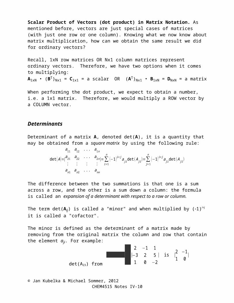
The minor is defined as the determinant of a matrix made by removing from the original matrix the column and row that contain the element aji. For example:
det(A23) from
|2 −1 1−3 2 51 0 −2
| is |2 −11 0
|
Example : The determinant of a 3x3 matrix:
det (A )=det(a11 a12 a13
a21 a22 a23
a31 a32 a33)=a11(−1)2 det (a22 a23
a32 a33 ) +a12(−1 )3det(a21 a23
a31 a33)+a13(−1 )4 det(a21 a22
a31 a32)
Each of the 2x2 determinants can be solved using the same technique. For example:
det (A11)=det(a22 a23
a32 a33)=a22(−1 )4 det (a33 )+a23(−1)5 det (a32)
where the determinant of a 1x1 matrix (i.e. a number) is the value of the element, e.g.det (a33 )=a33
giving:
det(a22 a23
a32 a33)=a22a33−a23 a32
which is the same as the following easy rule for any 2 x 2 determinant:
det(a bc d )=ad−bc
Any row or column could have been used as the starting point, for example, if the second column were used instead of the first row, the determinant would be:
det (A )=det(a11 a12 a13
a21 a22 a23
a31 a32 a33)=a12(−1 )3 det(a21 a23
a31 a33 ) +a22(−1 )4 det(a11 a13
a31 a33)+a32(−1)5 det (a11 a13
a21 a23)
In practice, it is best to pick one that has most zeros; it will greatly shorten and simplify the calculation!
1. Everything said about rows (or columns) applies equally to columns (or rows).
2. Expansion about a row (or column): if all elements except one in a row (or column) are zero, the determinant equals the product of that element by its cofactor (see definition of determinant and example above). In particular, if all elements of a row (or column) are zero the determinant is zero!
3. The value of a determinant remains the same if rows and columns are interchanged:det(A) = det(AT)
4. An interchange of any two rows (or columns) changes the sign of the determinant.
5. If all elements of any row (or column) are multiplied by a constant the determinant also multiplied by that constant.
6. If A is an n n matrix and c is a constant:det(cA) = cn det(A)
7. If any two rows (or columns) are the same or proportional (linearly dependent) the determinant is zero.
8. If elements of any row (or column) are multiplied by a number and added to another row (column) the value of the determinant remains the same (i.e. making a linear combination of rows or columns does not change the determinant).
9. If A, B are square matrices of the same order:det(AB) = det(A) det(B)
10. If v1, v2, …vn are row (column) vectors of an n n square matrix. Then det (A) = 0 if there exist scalar constants 1, 2, … n, such that:
1v1 + 2v2+ …+ nvn = 0
This condition is the same as saying that one of the vectors can be expressed as a linear combination of the other vectors, e.g.
v1 = (2/1)v2 + (3/1)v3 +…+ (n/1)vn = 0which, as we already know, means that the vectors are linearly dependent. Otherwise they are linearly independent. In other words if an n n matrix does not have n linearly independent rows or columns, its determinant is zero. Such matrix is called singular matrix. Otherwise it is called a non-singular or regular matrix.
Singular Matrix: A matrix is said to be singular if its determinant is 0. As we will see later, singular matrices have no inverse.
Matrix rank: The rank of a matrix A is the maximal number of linearly independent rows (or columns) of A.
The maximum rank of an mxn matrix is the minimum of m and n. A matrix that has a rank as large as possible is said to have full rank; otherwise, the matrix is rank deficient.
For a square matrix (nxn): if it has rank n is non-singular and its determinant is non-zero; if its rank < n, it is singular (determinant is zero).
3-D Vector Cross Product as a determinant: One of the most common uses of determinants is as mnemonic device to remember the cross product of 3 dimensional vectors. The vectors are written as the second and third rows of a 3x3 matrix. The first row is made up of the 3 unit
vectors (i.e. i , j , k ), and the cross product is calculated by evaluating the determinant using the first row as the starting point. In other words:
A×B=det( i j kxA y A z A
xB yB zB)= i det( y A z A
y B zB)− j det(x A z A
xB zB)+ k det(x A y A
xB yB)
= i ( y A z B−z A yB )− j ( x A z B−z A x B )+k (x A yB− y A x B)
Trace of a matrix
In linear algebra, the trace of an n × n square matrix A is defined to be the sum of the elements on the main diagonal (the diagonal from the upper left to the lower right) of A, i.e.,
Tr ( A )=a11+a22+. ..+ann=∑i=1
n
a ii
Properties of matrix trace:
1. Tr(A+B) = Tr(A) + Tr(B)
2. Tr(cA) = cTr(A)
3. If A is m × n and B is n × m then: Tr(AB) = Tr(BA)
4. A matrix and its transpose have the same trace: Tr(AT) = Tr(A)
Matrix inverse
Division of Matrices and Matrix Inverse: When we talked about operations with matrices, we have not covered matrix division. Division of a matrix A by a matrix B can be defined as multiplication of A by the inverse matrix of B or B-1. Since matrix multiplication is not commutative, we can have two different divisions - left and right:
A/B = A•B–1
A\B = A–1•Bwhere the inverse matrix B-1 is defined as:
where I is the unit matrix. Just like the matrix multiplication, the dimensions have to be right for these operations to make sense. Furthermore, the inverse matrix B1 must exist. This is true only for a non-singular, square matrix, i.e. if det(B) 0 ! This is important, so let’s say it again:
If A is non-singular square matrix, i.e. det(A) 0 there exists a unique inverse A1 so thatA–1 • A = A • A–1 = I
Important properties of the inverse:1. (A • B)-1 = B–1•A–1
2. (A–1) –1 = A
How do we determine the inverse of a Matrix? There are two methods: the row reduction method and using determinants. Both are practical only for small matrices, for large ones you generally need a computer.
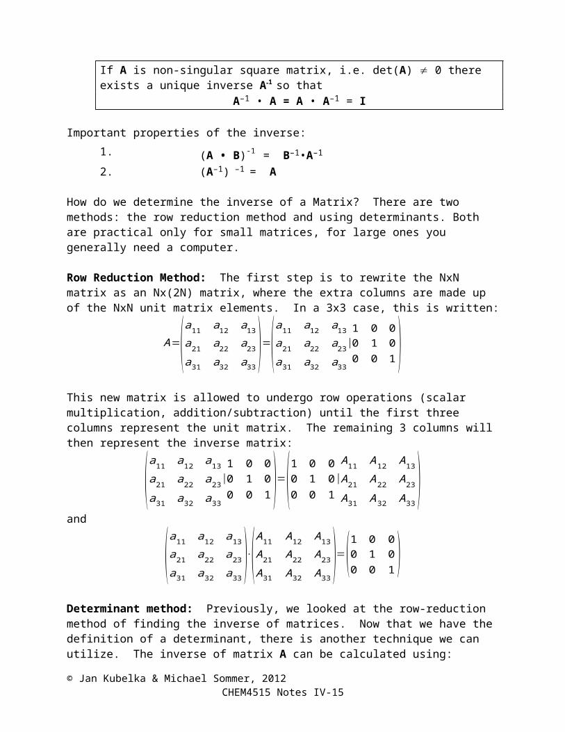
Row Reduction Method: The first step is to rewrite the NxN matrix as an Nx(2N) matrix, where the extra columns are made up of the NxN unit matrix elements. In a 3x3 case, this is written:
A=(a11 a12 a13
a21 a22 a23
a31 a32 a33)=(a11 a12 a13
a21 a22 a23
a31 a32 a33
|1 0 00 1 00 0 1 )
This new matrix is allowed to undergo row operations (scalar multiplication, addition/subtraction) until the first three columns represent the unit matrix. The remaining 3 columns will then represent the inverse matrix:
(a11 a12 a13
a21 a22 a23
a31 a32 a33
|1 0 00 1 00 0 1 )=(1 0 0
0 1 00 0 1
|A11 A12 A13
A21 A22 A23
A31 A32 A33)
and
(a11 a12 a13
a21 a22 a23
a31 a32 a33)⋅(A11 A12 A13
A21 A22 A23
A31 A32 A33)=(1 0 0
0 1 00 0 1 )
Determinant method: Previously, we looked at the row-reduction method of finding the inverse of matrices. Now that we have the definition of a determinant, there is another technique we can utilize. The inverse of matrix A can be calculated using:
A−1=(A jk )
T
det (A )where Ajk is the matrix of cofactors. This equality can be rearranged to give:
3. For an orthogonal matrix A, |det(A) | = 1, therefore det(A) is either +1 or 1.
Example:
The rotation matrix R=(cosθ sin θ
−sinθ cosθ ) is orthogonal.
Generalized inverse (Pseudo-inverse)
Rectangular matrices do not have an inverse (because determinant is always zero). However, rectangular matrices can be inverted in a generalized sense using pseudo-inverses. Recall that for any matrix A, the multiplication by its transpose AT (from either left or right) produces a square matrix. If this square matrix is regular, its inverse can be calculated. Then we say that the matrix has a left or right pseudo-inverse.
How can we tell which one can the matrix possibly has? Whichever of AT •A or A • AT gives the lower dimension square matrix has a chance of being regular (the one which gives the larger dimension matrix will not be regular for sure).
In other words, for an m n matrix A the square matrix AT •A will be n n and A • AT m m. If m > n the AT •A matrix is the lower dimension one (n n), and left pseudo-inverse may exist, such that:
(AT •A)-1 •(AT •A) =[(AT •A)-1 •AT] •A= In where In is an n n unit matrix.
The n m matrix [(AT •A)-1 •AT] is called the left pseudo-inverse, because it multiplies A from the left and gives the unit matrix.
If, on the other hand, m < n the right pseudo-inverse may exist:(A •AT) • (A •AT)-1 = A •[AT • (A •AT)-1] = Im
and [AT • (A •AT)-1] is the right pseudo-inverse of A, because it comes from the right.
Example: Find a pseudo-inverse for
This matrix is 3 2 and, so that an inverse for (2 2) matrix ATA may exist and therefore a left pseudo-inverse (2 3) of A may exist:
AT A=(21 11
−10 )( 2
1−1
110)=(6 3
3 2 )( AT A )−1=(6 3
3 2 )−1=(2 /3 −1
−1 2 ) (using, for example, the determinant method)
where A is an m n matrix, x is an n 1 matrix (column vector with n elements) and b is an m 1 matrix (column vector with m elements). This represents a completely general case of m equations of n unknowns. A special case where all b are zero:
The goal is to find the solution, i.e. the vector x which satisfies the above system or, equivalently, the matrix equation. Depending on what the A and b are, several general statements can be made about the possible solutions. It is helpful to define a so called augmented matrix where the right hand side b is added to A:
( A|b )=(a11 a12 . .. a1n
a21 a22 . .. a2n
⋮ ⋮ ⋮ ⋮am1 am2 . .. amn
|
b1
b2
⋮bn)
Now we can distinguish several important cases:
1. Non-homogeneous systems (b not all zeros).
a) m = n: the same number of equations as unknowns. If all the equations are independent, i.e. rank of A = rank of (A|b) is n, then there is a unique solution
x = A-1•b(Note that this is the same case as if m > n, but rank of A = rank of (A|b) = n, where n is the number of variables. It would still represent n independent equations of n unknowns, but we would have to use a pseudo-inverse, as true matrix inverse would not exist).
b) m > n: more equations than unknowns. This is known as an over-determined system. Strictly there may be no solution that exactly satisfies all the equations. However, the equations can be solved in the ‘least squares sense”, i.e. by x whose square differences from the exact solution to each equation are minimal. This is done by the left pseudo-inverse:
x = A-1•b, where A-1 = [(AT •A)-1 •AT]
c) Non homogeneous m < n or m = n but rank of A = rank of (A|b) < n unknowns. Fewer equations than unknowns. This is known as an underdetermined system, because there are not enough conditions to “fix” all the variables. There is an infinite number of solutions, where we are free to specify one or few of the x components and the remaining ones are determined by the equations. How many we can specify depends on the number of independent equations (rank) and the number of variables. For example 3 independent equations and five variables can be satisfied by choosing two variables independently and calculating the remaining three from the equations.
d) Non homogeneous m < n or m = n, rank of A < rank of (A|b). There is no solution.
2. Homogeneous systems (b = 0).
a) There is always a trivial solution x = 0
b) For n n homogeneous system the condition for a non-trivial solution of the homogeneous equation
A•x = 0to exist is that the A is singular matrix, i.e.
det(A) = 0This is an extremely important condition and the last equation is called a secular equation.
c) If the non trivial solution exists, there will be an infinite number of them because the system is underdetermined, i.e. the equation are linearly dependent and there is more unknowns that independente equations. The solution with some variables chosen independently may be found as in c) for non-homogeneous systems. A unique solution may be found by specifying additional conditions, e.g. normalization. We will see examples when we get to eigenvalue problems.
d) If det(A) 0 the only solution is the trivial solution (x = 0).
Cramer's Rule: The determinant can be used to find the solutions to a system of n non-homogeneous linear equations that have n variables. The technique, known as Cramer's rule, involves solving the determinant of the coefficient matrix and the determinant of a series of matrices constructed by replacing the variable's column by the solutions. An example will help illustrate the technique.
Example: Let’s look at the system of equations that satisfy the equation:
All the elements in the first column represent coefficients of x. The solutions to the equations are:
x1=det ( A1 )det ( A )
, x2=det ( A2)det ( A )
, x3=det( A3 )det( A )
where
det (A )=det(a11 a12 a13
a21 a22 a23
a31 a32 a33) , det( A1 )=det(b1 a12 a13
b2 a22 a23
b3 a32 a33)
det (A2 )=det(a11 b1 a13
a21 b2 a23
a31 b3 a33) , det( A3 )=det(a11 a12 b1
a21 a22 b2
a31 a32 b3)
Note that for this to work, det(A) must be nonzero.
Eigenvalues and Eigenvectors:
There are special cases of operators (matrices) that when they operate on a specific set of vectors the solution is the exactly the same vector, just multiplied by a constant. The set of vectors and corresponding constants are referred to as eigenvectors and eigenvalues of the matrix or operator. Symbolically, this is written:
A⋅X=λXor
(a11 a12 . .. a1n
a21 a22 . .. a2 n
⋮ ⋮ ⋮ ⋮an1 an 2 . .. ann
)(x1
x2
⋮xn)=λ (
x1
x2
⋮xn)
In order to perform the multiplication by a vector, we can notice that we can multiply the scalar by the elements of a unit matrix of the appropriate dimension:
Therefore, the matrix formed by the subtraction of the eigenvalue from the diagonal elements of the operator leads to a homogeneous system of equations.
Note that while the form of the equation (i.e. the matrix A) is known, the eigenvalues and the eigenvectors vectors are not! We therefore have n equations for n +1 unknowns (n components of the eigenvector xi and the eigenvalue ). How can we determine the eigenvalues and eigenvectors simultaneously?
Recall that for a homogeneous equation to have a non-trivial solution (i.e. not all xi equal to zero) the determinant of the matrix has to be equal zero (previous section, rule 2.b). Therefore, the above equation has non trivial solutions if and only if:
det(a11−λ a12 . . . a1n
a21 a22−λ . . . a2n
⋮ ⋮ ⋮ ⋮an 1 an 2 . . . ann− λ )=0
which can be also written as
det ( A−λ I )=0
This equation is called a secular equation. It leads to a polynomial of degree n, whose n roots are the eigenvalues. The polynomial equation, which follows from det (Â – Î) =0 by solving the determinant (for example by expansion along a row or a column) is called the characteristic equation.
Solving the characteristic equation therefore leads to n eigenvalues k ( k = 1, 2, …n ). Corresponding to each of the eigenvalues k will be an eigenvector Xk, which will be a non-trivial solution of the equation:
(a11−λk a12 . .. a1 n
a21 a22−λk . .. a2 n
⋮ ⋮ ⋮ ⋮an1 an 2 . .. ann−λk
)(x1
k
x2k
⋮xn
k )=(00⋮0)Example
: Find eigenvalues and eigenvectors of the following matrix: A=( 1 −2
−2 4 )
Characteristic equation of det ( A−λ I )=0 is:λ2−5 λ+0=0
with solutions, i.e. eigenvalues: λ1=0 , λ2=5
To find eigenvectors, substitute back to the matrix equation:
chose one of the variables and get the other one), so a possible eigenvector would be
x1= 1√5 (21)
where the prefactor 1/√5makes the vector normalized.
The other eigenvector for =5
(1−5 −2−2 4−5 )(x1
1
x21 )=0
−4 x11−2 x2
1=0−2x1
1−x21=0
which is solved by x11=−1/2 x2
1and the eigenvector would be:
x2= 1√5 ( 1
−2)
Theorems regarding eigenvalues and eigenvectors:
1. Eigenvalues of a Hermitian matrix are real.2. Eigenvalues of a unitary matrix (or its special case real orthogonal matrix) all have absolute value equal to one.3. Eigenvectors belonging to different eigenvalues of a Hermitian matrix (or its special case real symmetric matrix) are orthogonal
Coordinate Transformations:
We have already seen how we can transform, for example, (x, y, z) to (r, , ) using certain geometric equivalences. A similar process can be done to convert any arbitrary set of coordinates to a new, more convenient set of coordinates. Rotating the coordinate system to fit a particular case often does this. In terms of matrix operations, we can define a rotation matrix, R, that operates on a position vector, a, to give a rotated vector, a'.
Example: Rotation in 2-D. Find the matrix R that would rotate a vector by an angle .
Rotating a vector by is the same as rotating the coordinate system by in the opposite direction. (Remember the angles are oriented and therefore have signs: by convention rotation in the counter clockwise direction is positive, and clockwise in negative). So we do not write + or the sign comes from the sense of the rotation.
Let’s represent the the original (before rotation) system by unit vectors i and j and the vector as a = xi + yj. In the new (rotated) system i', j' the vector will be a’ = x’i' + y’j'.
One way to do this would be to use trigonometry. This, however, is quite tedious. Better way (which a smart person familiar with the vector algebra would take) is to use projections. Remember that coordinates are just projections on the system unit vectors. The vector a’ in the old system would therefore be:
a'x = x' = ai' = (xi + yj) i' = xii' + yji'
But (see figure):ii' = cos and ji' = cos(/2sin
therefore:x' = xcos ysin
The same goes for the other component:a'y = y' = aj' = (xi + yj) j' = xij' + yjj'
= xsin +ycos
All together we have:x' = xcos ysiny' = xsin +ycos
Or:
(x '
y' )=(cos (θ ) −sin (θ )sin (θ ) cos (θ ) )( x
y )The rotation matrix is, therefore:
R=(cos (θ ) −sin (θ )sin (θ ) cos (θ ) )
Just as vectors may be represented by coordinates, which are projections on the unit vectors in the system axes, so can be matrices. However, because matrices are two dimensional, each element needs two projections:
A=(a11 a12 a13
a21 a22 a23
a31 a32 a33) can be written as:
a11 i i+a12 i j+a13 i k+A= a21 j i+a22 j j+a23 j k+
a21k i+a22 kj+a23k k+
Just like we discussed for vectors, the matrix elements (coordinated of a matrix ) are also dependent on the coordinate system ( i, j, k). In a different coordinate system, the elements would have different values, in analogy to the vector components.
As se have just seen, vectors can be transformed between different coordinate systems by a transformation matrix:
a' = Ra
For matrices, since we have two indices, the transformation must involve the matrix twice. Exact derivation shows that the transformation of the basis for a matrix has the form:
A' = R–1 A R where A' is the matrix in the “new” basis (e.g. rotated by an angle) and R is the rotation matrix, just like above (R–1 is, of course, it inverse).
Diagonalizing Matrices:
Now let’s go back to the eigenvalue problem. For each eigenvalue/eigenvector we have:Âxk = xk
If we construct a matrix of eigenvectors X which will have each eigenvector (xk ) as a column, we can write this in matrix form :
(a11 a12 . .. a1n
a21 a22 . .. a2 n
⋮ ⋮ ⋮ ⋮an1 an 2 . .. ann
)(x1
1
x21
⋮xn
1
x12
x22
⋮xn
2
. ..
. ..⋮. ..
x1n
x2n
⋮xn
n )=(x1
1
x21
⋮xn
1
x12
x22
⋮xn
2
. ..
. ..⋮. ..
x1n
x2n
⋮xn
n)(λ1
0⋮0
0λ2
⋮0
. ..
. ..⋮. ..
00⋮λn)
orÂX = X
where is a diagonal matrix (with eigenvalues on the diagonal and zeros elsewhere).
It is important to keep in mind that each eigenvector has its own corresponding eigenvalue! Note that the eigenvectors in matrix X have to be ordered, i.e. the first column is the eigenvector one corresponding to the first eigenvalue position 1,1 in the eigenvalue matrixthe second column to the second one(2,2 position) etc. If you mix them up it is not going to work!
Now multiply this equation from the left by X–1:X–1ÂX = X–1X
X–1ÂX =
We have therefore reduced the matrix to a diagonal form, where all the elements except the diagonal are zero. Now recall that X–1ÂX is just a form of coordinate transformation. The coordinates we have just transformed the matrix to, however, are special: they are its own eigenvectors.
In the basis of its eigenvectors the matrix is diagonal. The diagonal elements are the eigenvalues.
Important special cases arise if the matrix A is Hermitian (or symmetric, in the real case). Then the eigenvalues are always real and the eigenvectors are orthogonal! Since the eigenvectors are orthogonal, the matrix X in the transformation above is a unitary matrix, whose special case (real
numbers) is the orthogonal matrix. Recall that for an orthogonal matrix the inverse equals its transpose, so that:
X†ÂX = or, for real matrices:
XTÂX =
These are called unitary (orthogonal) transformation, and correspond to the transformation of coordinates, rotations of the system etc. Since the absolute value of the determinant of a unitary (orthogonal) matrix is always one, these transformations are also called “norm preserving”: i.e. they will not change lengths of any vectors, only “rotate’ them.
Similar Matrices.
Matrices related by a coordinate transformationT–1ÂT =
are called similar matrices. Several important relationships between similar matrices follow from the rules for calculating traces and determinants:
1. Tr(T–1ÂT) = Tr() = Tr() 2. det(T–1ÂT) = det(B) = det() 3. rank(T–1ÂT) = rank(B) = rank() 4. Similar matrices have the same eigenvalues (though eigenvectors are generally different).
Important special cases, again, are matrices related by the unitary (orthogonal) transformation.
Functions of matrices
We know how to calculate a square of a matrix, or third and higher power of it. But can we calculate, for example a square root, exponential, logarithm or sin of a matrix? It turns out we can define arbitrary functions of matrices based on the square, third etc. powers. Remember the Taylor series? That is precisely what we use to define functions of matrices:
f (A )=f (0 )+ f '( 0)⋅A+12
f ' '(0 )⋅A2+13 !
f ' ' ' (0)⋅A3+. .
= f (0)+ f ' (0 )⋅A+12
f ' ' (0)⋅A⋅A+13 !
f ' ' ' (0 )⋅A⋅A⋅A+. ..
Because we can multiply matrices, we can calculate 2nd, 3rd etc. powers and therefore, in principle, we can calculate any function of a matrix. The problem of course is that we would have to sum the Taylor series up to infinity. However, we can completely avoid it, using what we have just learned about matrix diagonalization and similar matrices. Using:
X–1AX = where is diagonal matrix of eigenvalues and X is the matrix of eigenvectors, A can be written (by multiplying by X from left and X–1 from right):
Notice that X–1X = I and any matrix multiplied by I equals itself, and therefore we have:
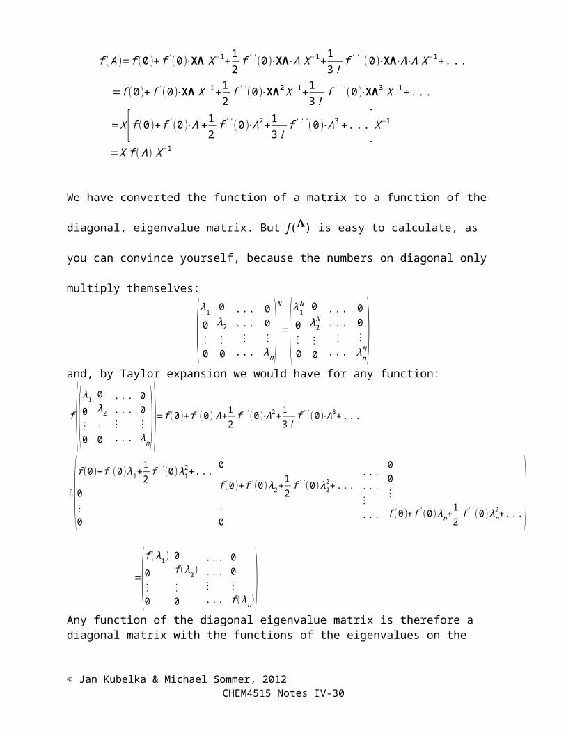
f (A )=f (0 )+ f '( 0)⋅XΛ X−1+12
f ' ' (0 )⋅XΛ⋅Λ X−1+13 !
f ' ' ' (0)⋅XΛ⋅Λ⋅Λ X−1+. . .
= f (0)+ f ' (0 )⋅XΛ X−1+12
f ' ' (0 )⋅XΛ2 X−1+13 !
f ' ' ' (0 )⋅XΛ3 X−1+. ..
=X [ f ( 0)+ f '( 0)⋅Λ +12
f ' ' (0)⋅Λ2+13 !
f ' ' ' (0 )⋅Λ3 +.. .]X−1
=X f ( Λ) X−1
We have converted the function of a matrix to a function of the diagonal, eigenvalue matrix. But
f() is easy to calculate, as you can convince yourself, because the numbers on diagonal only
multiply themselves:
(λ1
0⋮0
0λ2
⋮0
. . .
. . .⋮
. . .
00⋮λn)
N
=(λ1N
0⋮0
0λ2
N
⋮0
.. .
.. .⋮.. .
00⋮λn
N)and, by Taylor expansion we would have for any function:
f (( λ1
0⋮0
0λ2⋮0
.. .
.. .⋮.. .
00⋮λn))=f (0 )+ f ' (0 )⋅Λ+1
2f ' ' (0 )⋅Λ2+1
3!f ' ' (0)⋅Λ3+. . .
¿( f (0 )+ f '(0 ) λ1+12
f ' '(0 ) λ12+. . .
0⋮0
0
f (0 )+ f ' (0 )λ2+12
f ' ' (0 )λ22+. ..
⋮0
. ..
. ..⋮. ..
00⋮
f (0)+ f ' (0) λn+12
f ' ' (0 )λn2+. ..)
=(f ( λ1 )0⋮0
0f ( λ2 )⋮0
.. .
.. .⋮.. .
00⋮f ( λn )
)Any function of the diagonal eigenvalue matrix is therefore a diagonal matrix with the functions of the eigenvalues on the diagonal! This is a remarkable result, because it allows us to calculate functions of matrices. Putting it all together:
where X is the matrix of eigenvectors and X-1 its inverse. To calculate a function of a matrix,
you have to:
1. Calculate eigenvalues and eigenvectors
2. Build the eiganvalue and eigenvector matrices (remember the ordering - k-th
column in the eigenvector matrix is the eigenvector corresponding to k-th eigenvalue,
i.e. the value in position k,k in the eigenvalue matrix.) and find the inverse of the
eigenvector matrix.
3. Calculate the function of the eigenvalues and put them on the diagonal
4. Do the multiplications X f ( Λ ) X−1
Example: Exponential of a matrix.
Matrix exponentials are important, because they can be used to solve systems of first order differential equations (as we’ll see later). In general (from above) the matrix exponential is calculated as:
exp( A )=X⋅(exp( λ1)
0⋮0
0exp( λ2)
⋮0
. ..
. ..⋮. ..
00⋮
exp ( λn ))⋅X−1
as an example we try to calculate exponential of A=( 1 −2
−2 4 ) whose eigenvalues and
eigenvectors we already found above:
Λ=(0 00 5 ) , X= 1
√5 (2 11 −2 ) , X−1= XT= 1
√5 (2 11 −2 )
The eigenvector matrix is orthogonal, so it is really easy to find its inverse. But it is also always a good idea to check that the inverse is right:
In the MATLAB environment, a matrix is a rectangular array of numbers. Special meaning is sometimes attached to 1-by-1 matrices, which are scalars, and to matrices with only one row or column, which are vectors and, as we have already seen, vectors can represent functions. In general, all the mathematical (numerical) data can be thought of as matrices.
The operations in MATLAB are designed to be as natural as possible. Where other programming languages work with numbers one at a time, MATLAB allows you to work with entire matrices quickly and easily.
Entering Matrices
You can enter matrices into MATLAB in several different ways:
1. Enter an explicit list of elements.2. Load matrices from external data files.3. Generate some special matrices using built-in functions.
We will start by entering a matrix as a list of its elements. You already know how to enter an array (a row vector). To enter a matrix, you only need to know how to separate multiple rows. Here are the rules:
1. Separate the elements of a row with blanks or commas.2. Use a semicolon, ; , to indicate the end of each row.3. Surround the entire list of elements with square brackets, [ ].
To enter a matrix, simply type in the Command Window
>>A = [16 3 2 13; 5 10 11 8; 9 6 7 12; 4 15 14 1]
MATLAB displays the matrix you just entered:
A =16 3 2 13 5 10 11 8 9 6 7 12 4 15 14 1
Just as any array or number, once you have entered the matrix, it is automatically remembered in the MATLAB workspace. You can refer to it simply as A.
Special matrices
MATLAB software provides four functions that generate basic matrices.zeros(n,m) n by m matrix of all zerosones(n,m) n by m matrix of all ones
rand(n,m) n by m matrix of random numbers between 0 and 1randn(n,m) n by m matrix of normally distributed random numbers (mean 0, standard deviation 1)
We have already encountered the load function. The load function reads binary files containing matrices generated by earlier MATLAB sessions, or reads text files containing numeric data. The text file should be organized as a rectangular table of numbers, separated by blanks, with one row per line, and an equal number of elements in each row. For example, outside of MATLAB, create a text file containing these four lines:
Save the file as my_matrix.txt in the current directory. The statement load my_matrix.txt reads the file and creates a variable, my_matrix, containing the example matrix. An alternative form of the load command is
Then the data in the file is loaded and assigned to a variable A. Remember to use single quotes for your file name.
Subscripts
You already know subscripts from indexing arrays (points on your function plots, etc.). The element in row i and column j of A is denoted by A(i,j). For example, A(4,2) is the
number in the fourth row and second column. For the magic square, A(4,2) is 15. So to compute the sum of the elements in the fourth column of A, type
>>A(1,4) + A(2,4) + A(3,4) + A(4,4)
This subscript produces:
ans = 34
but is not the most elegant way of summing a single column. It is also possible to refer to the elements of a matrix with a single subscript, A(k). A single subscript is the usual way of referencing row and column vectors (i.e. arrays, as we already know). However, it can also apply to a fully two-dimensional matrix, in which case the array is regarded as one long column vector formed from the columns of the original matrix. So, for the magic square, A(8) is another way of referring to the value 15 stored in A(4,2). If you try to use the value of an element outside of the matrix, it is an error:
>> t=A(4,5)??? Attempted to access A(4,5); index out of bounds because size(A)=[4,4].
Conversely, if you store a value in an element outside of the matrix, the size increases to accommodate the new number:
However, there is a better way to perform this computation. The colon by itself refers to all the elements in a row or column of a matrix. To calculate the sum of the fourth column, we can simply write:
>> sum(A(:,4))ans = 34
We can also use the keyword end to refer to the entire last row or column. For example the sum of the last column would be:
sum(A(:,end))ans = 34
and of the last row:
>> sum(A(end,:))ans = 37
This has an important application when dealing with external data. Data are often stored as columns of a matrix. For example, assume I have a radiation density of the blackbody (Planck law) as a function of frequency for four different temperatures (500K, 1000K, 1500K, 2000K) in a file, called planck.txt that may look like this:
where the first column is the frequency (in Hz), the second column the radiation density (in J.s.m3) for 500K, the third column for 1000K, fourth at 1500K and the last at 2000K. Suppose I want to load and plot the data. First load the file:
Now nu, r500, r1000 etc. are vectors then can be plotted as you are already familiar with:
>> plot(nu,r500)>> hold on>> plot(nu,r1000,':r')>> plot(nu,r1500,'--g')>> plot(nu,r2000,'+-k')
giving:
An even shorter way to do this would be:
>> hold off>> plot(r(:,1),r(:,2:end))
In this case, we are plotting one x (first column of r r(:,1)) and many different y, which are specified by a range of columns r(:,2:end). MATLAB will automatically pick a different color for each (unless you specify otherwise).
Using this simple procedure you can read and process any kind of (unformatted) data. For example, I can easily calculate the maxima (all at the same time):
Because max will find maxima of all columns and return them (and their indices) in row vectors. Theindeces (imax) can be used to find where the maxima are (as you already know for single variable functions) by finding these indices in the nu:
Concatenation is the process of joining small matrices to make bigger ones. In fact, you made your first matrix by concatenating its individual elements. The pair of square brackets, [ ], is the concatenation operator. For an example, start with the 4-by-4 matrix A from your file my_matrix.txt and formB = [A A+32; A+48 A+16]:
However, using a single subscript deletes a single element, or sequence of elements, and reshapes the remaining elements into a row vector:
>> X(2:2:10)=[]X = 16 9 2 7 13 12 1
transpose and diag()
The matrix A we have saved in our file is a “magic square”, which has some interesting properties. If you take the sum along any row or column, or along either of the two main diagonals, you will always get the same number. Let us verify that using MATLAB. The first statement to try is
>>sum(A)
MATLAB replies with
ans = 34 34 34 34
You have computed a row vector containing the sums of the columns of A. Each of the columns has the same sum, 34. How about the row sums? MATLAB has a preference for working with the columns of a matrix, so one way to get the row sums is to transpose the matrix, compute the column sums of the transpose, and then transpose the result. For an additional way that avoids the double transpose use the dimension argument for the sum function. MATLAB has two transpose operators. The apostrophe operator (e.g., A') performs a complex conjugate transposition. It flips a matrix about its main diagonal, and also changes the sign of the imaginary component of any complex elements of the matrix. The dot-apostrophe operator (e.g., A.'), transposes without affecting the sign of complex elements. For matrices containing all real elements, the two operators return the same result. So
The sum of the elements on the main diagonal is obtained with the diag()function. The diag() when the argument is a matrix gives the diagonal elements as a vector:
>>diag(A)
produces
ans = 16 10 7 1
and
sum(diag(A))
gives
ans = 34
The other diagonal, the so-called antidiagonal, is not so important mathematically, so MATLAB does not have a ready-made function for it. But a function originally intended for use in graphics, fliplr, flips a matrix from left to right:
>>sum(diag(fliplr(A)))ans = 34
When the argument is a vector, the diag() function produces a matrix (n n where n is the length of the vector) with the vector on the main diagonal. This way diag()can be used to generate, for example, unit matrices (matrices that have ones on diagonal and zeros everywhere else):
Note that a matrix plus its transpose produces a symmetric matrix:
>> A+A'ans = 4 10 8 10 0 3 8 3 8
While matrix minus its transpose produces an anti-symmetric matrix (with zeros on the diagonal, as antisymmetric matrix must have)
>> A-A'ans = 0 -4 2 4 0 1 -2 -1 0
Multiplication of matrices:
>> A*Bans = 30 38 34 22 13 10 24 22 23
>> B*Aans = 11 6 12 62 9 36 44 17 46
Note that matrix multiplication is not commutative: A*B and B*A result in different matrices. Also note that the matrix dimensions have to be right for these operations to work.
>> A(:,end)=[]A = 2 3 7 0 3 1
>> A+B??? Error using ==> plusMatrix dimensions must agree.
>> A*B??? Error using ==> mtimesInner matrix dimensions must agree. >> B*Aans = 11 6 62 9 44 17
And note that multiplication of a matrix (not necessarily square) with its transpose produces a square symmetric matrix
It looks like we did not get a unit matrix, but we really did: numbers on the order of 10-16 are just the numerical “noise” (rounding errors etc.). This is a good example for realizing that on the computer everything has some finite precision (e.g. zero is good only to about 10-16).
What happens if we have a singular matrix? Let’s make the last column of S a linear combination of the first three:
Because for this matrix m > n, it should have a left pseudoinverse. The pseudoinverse matrix has to be n m (2 5 in this case), and give a unit matrix that is n n (2 2):
We could use inverse and pseudoinverse to solve systems of linear equations. But it is not necessary and it is much better and more efficient to use the left divide (backslash) operator.
It is not a bad idea to make sure the ranks of A and the augmented matrix (A|b) are consistent (besides it is a good exercise for concatenating matrices):
>> rank(A)ans = 3>> rank([A b])ans = 3
We have an exactly determined system and we could solve it by matrix inverse:
Notice that we get a vector x with three components x(1), x(2) and x(3), which correspond to x, y, z in the equation above.
We never do this in MATLAB in this way though. The reason is that exact calculation of the inverse is expensive. What we really have to do is matrix division
A\bwhich can be done more efficiently without explicit calculation of the inverse. We therefore use the left divide or backslash for this:
>> x=A\bx = -6.4068e-001 -6.9492e-001 6.8542e+000
It is extremely important to have the order right! You could switch A and b in the division and still get a result (by virtue that the dimensions correspond), but it would be wrong:
>> x=b\Ax = -6.8575e-002 -3.3289e-003 1.3915e-001
So never ever do this!
If we had an over-determined system, we could solve it using pinv, but, again, we never do that and use the backlash instead. For example:
So the pseudoinverse works, but we will always use the backslash:
>> x=A\bx = 1.0492e-001 4.4601e-001
An example of an over-determined system is a linear regression. Imagine I have the following data points:x=[0 1 2 3 4 5 6]; y=[1.5 0.3 0.85 0.1 1.9 4.3 8.0] and that I want to approximate them by a quadratic function: y = a2x2+a1x+a0. This can be written in the matrix form as:
(y1
y2
⋮yn)=(11⋮1
x1
x2
⋮xn
x12
x22
⋮xn
2)(a0
a1
a2)
and solved for the coefficients a2 , a1x and a0 (Note that x is not the unknown in this case - x are known, the unknowns are the coefficients, so don’t get confused).
These are my coefficients, corresponding , respectively, to the absolute, linear and quadratic term. I can set up the quadratic equation and make sure it fits my points:
>> yfit=a(1)+a(2)*x+a(3)*x.*x;>> hold on>> plot(x,yfit,'k')
This is how you can do a regression (fit) to any function that is linear in the coefficients: i.e. it does not have to be a linear function (quadratic that we just did is certainly not a linear function), but remember that the unknowns are the coefficients ak. As long as the function is linear in these coefficients, a simple backslash will work.
To calculate eigenvalues and eigenvectors, there is a function eig(). It has two outputs: first is the matrix of eigenvectors and second the diagonal matrix of eigenvalues.
We will try it on a Hermitian matrix H (we know that for a Hermitian matrix the eigenvalues should be real and eigenvectors orthogonal, so we can test it):
But how about the eigenvectors: are they orthogonal? We can figure that out by doing a few scalar products. Remember that for complex vectors, the norm is defined as:
|A| = A*Aso it is a scalar (dot) product but with a complex conjugate. Also remember that eigenvectors are columns of X.
Those are all very good zeros. Furthermore, the eigenvectors are normalized:
>> X(:,1)'*X(:,1)ans = 1.0000e+000
which makes X a unitary matrix. To test that, remember that the inverse of a unitary matrix equals its Hermitian conjugate. Therefore X† X should be a unit matrix:
which it indeed is, except for some numerical noise.
With eigenvalues and eigenvectors you can calculate any function of a matrix, as we discussed above. But since matrix exponential is so important, MATLAB has a dedicated function to do it, called expm(). To try it out, we will first show that exponential of a diagonal matrix is just the exponentials of its diagonal elements. To make this easy to see, I make the elements logarithms of 1, 2, 3 and 4:
where I made use of the fact that the eigenvectors of a symmetric matrix are orthogonal, and the inverse of the orthogonal matrix is the transpose. But even if I did not know it: