1 1 IV. MODELS FROM DATA 1 Data mining 2 Data mining MODELLING METHODS- Data mining data 3 Outline A) THEORETICAL BACKGROUND 1. Knowledge discovery in data bases (KDD) 2. Data mining • Data • Patterns • Data mining algorithms B) PRACTICAL IMPLEMENTATIONS 3. Applications: • Equations • Decision trees • Rules
Transcript
1
1
IV. MODELS FROM DATA
1
Data mining
2
Data mining
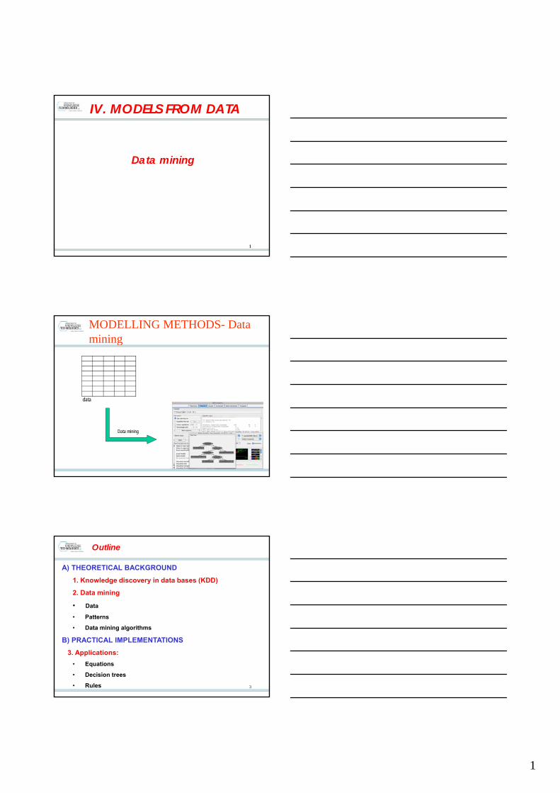
MODELLING METHODS- Data mining
data
3
Outline
A) THEORETICAL BACKGROUND
1. Knowledge discovery in data bases (KDD)
2. Data mining
• Data
• Patterns
• Data mining algorithms
B) PRACTICAL IMPLEMENTATIONS
3. Applications:
• Equations
• Decision trees
• Rules
2
4
Knowledge discovery in data bases (KDD)
What is KDD?
Frawley et al., 1991: “KDD is the non-trivial process of identifying valid, novel, potentially useful, and ultimately understandable patterns in data”,
How to find patters in data?
Data mining (DM) – central step in the KDD process concerned with applying computational techniques to actually find patterns in the data (15-25% of the effort of the overall KDD process).
- step 1: preparing data for DM (data preprocessing)
- step 3: evaluating the discovered patterns (results of DM)
5
Knowledge discovery in data bases (KDD)
When the patterns can be treated as knowledge?
Frawley et al., (1991): “A pattern that is interesting (according to
a user- imposed interest measure) and certain enough (again
according to the user’s criteria) is called knowledge. “
Condition 1: Discovered patterns should be valid on new data with some degree of certainty (typically prescribed by the user).
Condition 2: The patterns should potentially lead to some useful actions (according to user defined utility criteria).
6
Knowledge discovery in data bases (KDD)
What may KDD contribute to environmental sciences (ES) (e.g. agronomy, forestry, ecology, …)?
ES deal with complex unpredictable natural systems (e.g. arable, forest and water ecosystems) in order to get answers on complex questions.
The amount of collected environmental data is increasing exponentially.
KDD was purposively designed to cope with such complex questions about complex systems like:
- understanding the domain/system studied (e.g., gene flow, seed bank, life cycle, …)- predicting future values of system variables of interest (e.g., rate of out-crossing with GM plants at location x at time y, seedbank dynamics, …)
3
7
Data mining (DM)
What is data mining?Data Mining, is the process of automatically searching large
volumes of data for patterns using algorithms.
Data Mining – Machine learningData Mining is the application of Machine Learning techniques
to data analysis problems.
The most relevant notions of data mining:1. Data
2. Patterns
3. Data mining algorithms
8
Data mining (DM) - data
1. What is data?According to Fayyad et al. (1996):” Data is a set of facts, e.g., cases in a database.”
Data in DM is given in a single flat table:- rows: objects or records (examples in ML)- columns: properties of objects (attributes, features in ML)
which is then used as input to a data mining algorithm.
A pattern is defined as: ”A statement (expression) in a given language, that describes (relationships among) the facts in a subset of the given data and is (in some sense) simpler than the enumeration of all facts in the subset” (Frawley et al. 1991, Fayyad et al. 1996).
Classes of patterns considered in DM (depend on the data mining task at hand):
1. equations,2. decision trees3. association, classification, and regression rules
4
10
Data mining (DM) - pattern
1.EquationsTo predict the value of a target (dependent) variable as a linear or non linear combination of the input (independent) variables.
�Linear equations involving:- two variables: straight lines in a two dimensional space - three variables: planes in a three-dimensional space - more variables: hyper-plains in multidimensional spaces
�Nonlinear equations involving:- two variables: curves in a two dimensional space - three variables: surfaces in a three-dimensional space - more variables: hyper-surfaces in multidimensional spaces
11
Data mining (DM) - pattern
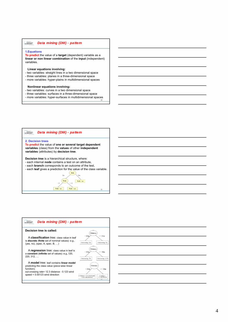
2. Decision treesTo predict the value of one or several target dependentvariables (class) from the values of other independentvariables (attributes) by decision tree.
Decision tree is a hierarchical structure, where: - each internal node contains a test on an attribute, - each branch corresponds to an outcome of the test, - each leaf gives a prediction for the value of the class variable.
12
Data mining (DM) - pattern
Decision tree is called:
� A classification tree: class value in leaf is discrete (finite set of nominal values): e.g., (yes, no), (spec. A, spec. B, …)
� A regression tree: class value in leaf is a constant (infinite set of values): e.g.,120, 220, 312, …
� A model tree: leaf contains linear modelpredicting the class value (piece-wise linear function): out-crossing rate= 12.3 distance - 0.123 wind speed + 0.00123 wind direction
5
13
Data mining (DM) - pattern
3. RulesTo perform association analysis between attributes discovered by association rules.
The rule denotes patterns of the form:“IF Conjunction of conditions THEN Conclusion.”
� For classification rules, the conclusion assigns one of the possible discrete values to the class (finite set of nominal values): e.g., (yes, no), (spec. A, spec. B, spec. D)
� For predictive rules, the conclusion gives a prediction for the value of the target (class) variable (infinite set of values): e.g.,120, 220, 312, …
14
Data mining (DM) - algorithm
3. What is data mining algorithm?Algorithm in general:- a procedure (a finite set of well-defined instructions) for accomplishing some task which will terminate in a defined end-stat.
Data mining algorithm:- a computational process defined by a Turing machine (Gurevich et al. 2000) for finding patterns in data
15
Data mining (DM) - algorithm
What kind of possible algorithms do we use for discovering patterns?
It depends on the goals:
1. Equations = Linear and multiple regressions
2. Decision trees = Top/down induction of decision trees
3. Rules = Rule induction
6
16
Data mining (DM) - algorithm
1. Linear and multiple regression
• Bivariate linear regression:predicted variable (C-class (ML) my be contusions or discontinues) can be expressed as a linear function of one attribute (A):
C = α+ β×A
• Multiple regression:predicted variable (C-class (ML) my be contusions or discontinues) can be expressed as a linear function of a multi-dimensional attribute vector (Ai):
C = Σni =1 βi×Ai
17
Data mining (DM) - algorithm
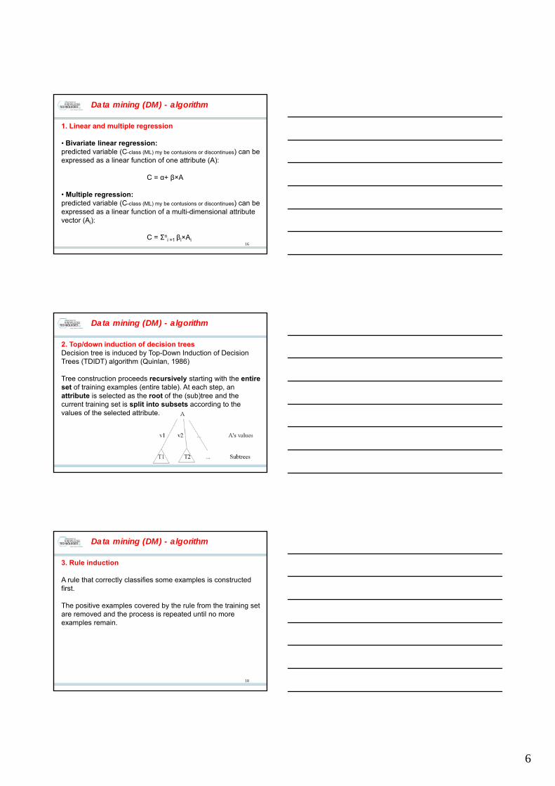
2. Top/down induction of decision treesDecision tree is induced by Top-Down Induction of Decision Trees (TDIDT) algorithm (Quinlan, 1986)
Tree construction proceeds recursively starting with the entireset of training examples (entire table). At each step, an attribute is selected as the root of the (sub)tree and the current training set is split into subsets according to the values of the selected attribute.
18
Data mining (DM) - algorithm
3. Rule induction
A rule that correctly classifies some examples is constructed first.
The positive examples covered by the rule from the training set are removed and the process is repeated until no more examples remain.
7
19
Data mining (DM) - Statistics
Data mining vs. statistics
Common to both approaches:
Reasoning FROM properties of a data sample TO properties of a population.
20
Data mining (DM) – Machine learning -Statistics
StatisticsHypothesis testing when certain theoretical expectations about the data distribution, independence, random sampling, sample size, etc. are satisfied.
Main approach: best fitting all the available data.
Data miningAutomated construction of understandable patterns, and structured models.
Main approach: structuring the data space, heuristic search for decision trees, rules, … covering (parts of) the data space.
2121
DATA MINING – CASE STUDIES
8
2222
Practical implementations
Each class of described patterns is illustrated with examples of applications:
2. Decision trees:• Classification trees• Regression trees• Model trees
3. Predictive rules
2323
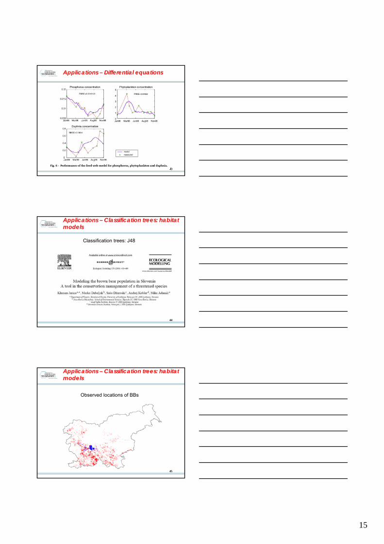
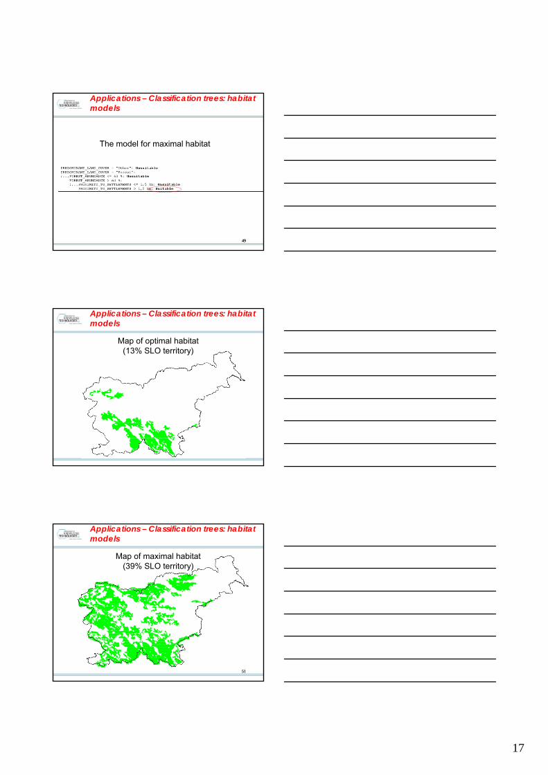
Applications – Difference equations
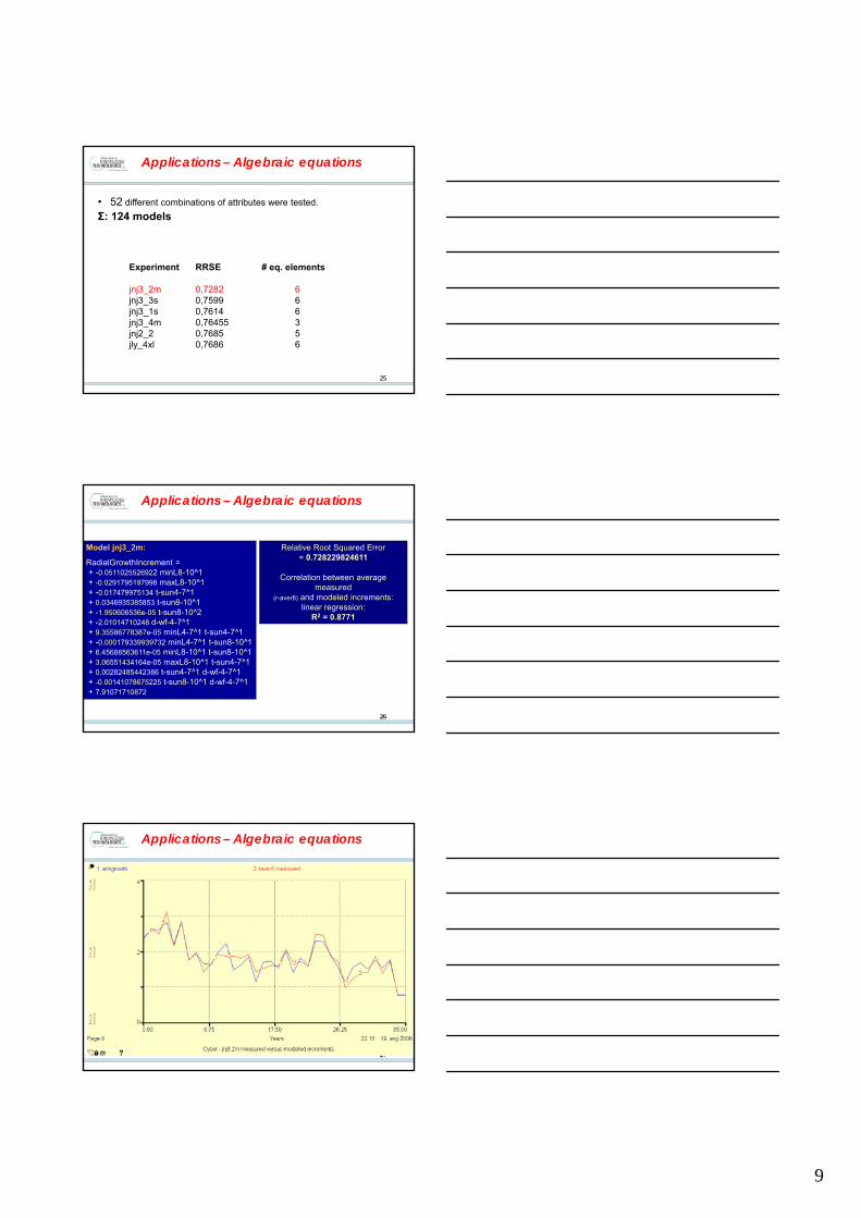
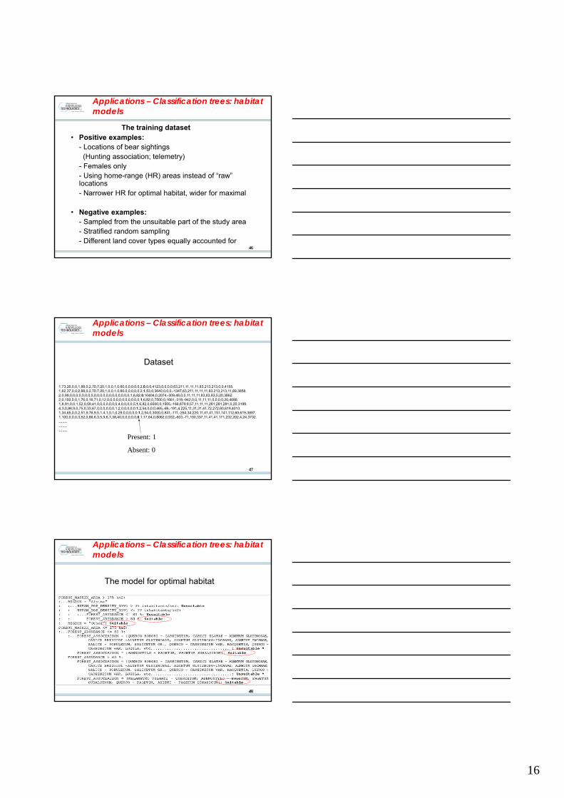
Algebraic equations: CIPER
2424
Applications – Algebraic equations
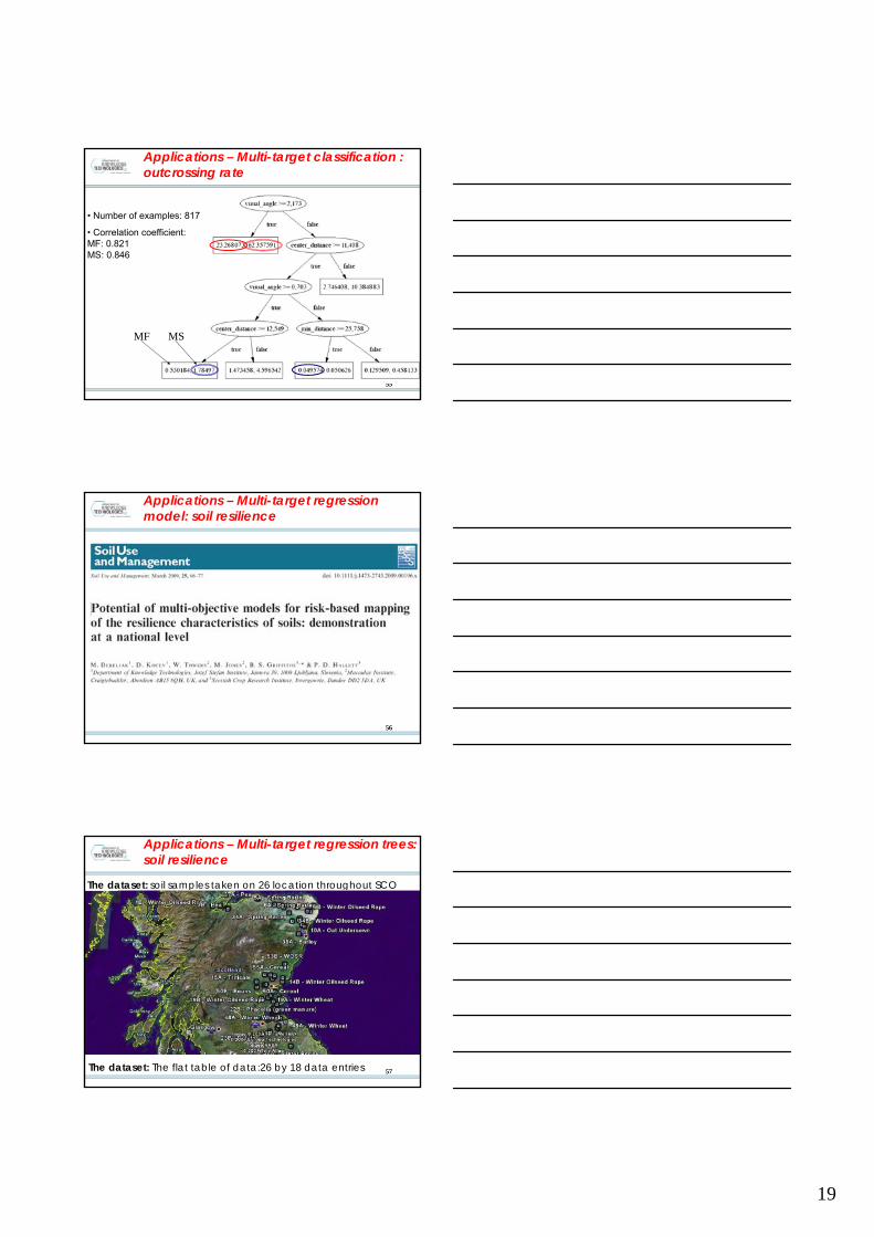
Dataset
Hydrological conditions(HMS Lendava; monthly data on
minimal, average and maximum values)
- Ledava River levels - groundwater levels
Meteorological conditions(monthly data, HMS Lendava):-Time of solar radiation (h), - precipitation (mm), - ET (mm)- Number of days with white frost - Number of days with snow- T: max, aver, min- Cumulative T>0ºC, >5ºC, and >10ºC- Number of days with:
Modelling pollen dispersal of genetically modified oilseed rape within the field
Marko Debeljak, Claire Lavigne, Sašo Džeroski,Damjan Demšar
In: 90th ESA Annual Meeting [jointly with the]IX International Congress of Ecology, August 7-12,2005, Montréal, Canada. Abstracts. [S.l.]: ESA, 2005, p.
152.
5353
Experiment design:
90m
90m
Donors: MF transgenic oilseed rape “B004.oxy”
(10×10m)
Filed for receptors (90×90m)
3×3m grid = 841 nodes
10 seeds of MS oilseed rape “FU58B004” planted per node
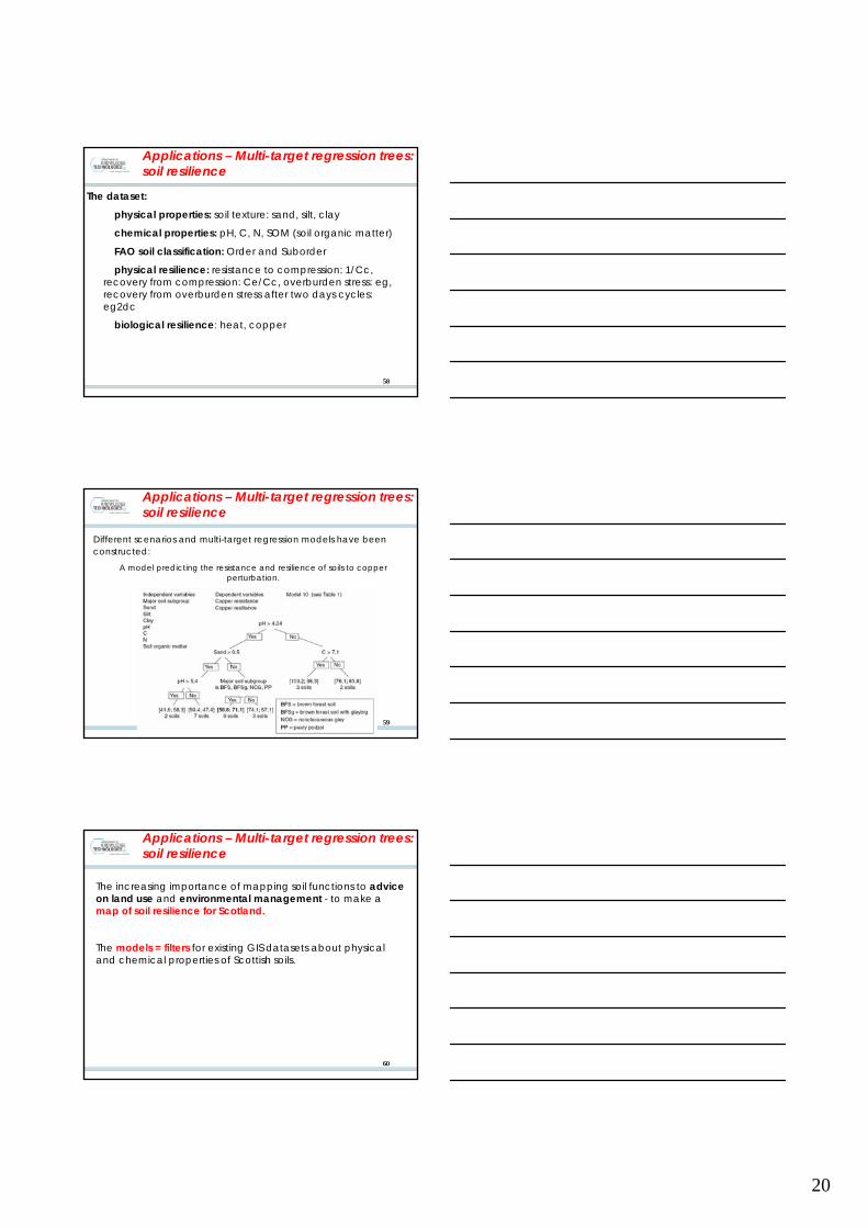
� chemical properties: pH, C, N, SOM (soil organic matter)
� FAO soil classification: Order and Suborder
� physical resilience: resistance to compression: 1/Cc, recovery from compression: Ce/Cc, overburden stress: eg, recovery from overburden stress after two days cycles: eg2dc
The increasing importance of mapping soil functions to advice on land use and environmental management - to make a map of soil resilience for Scotland.
The models = filters for existing GIS datasets about physical and chemical properties of Scottish soils.
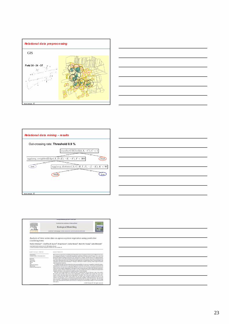
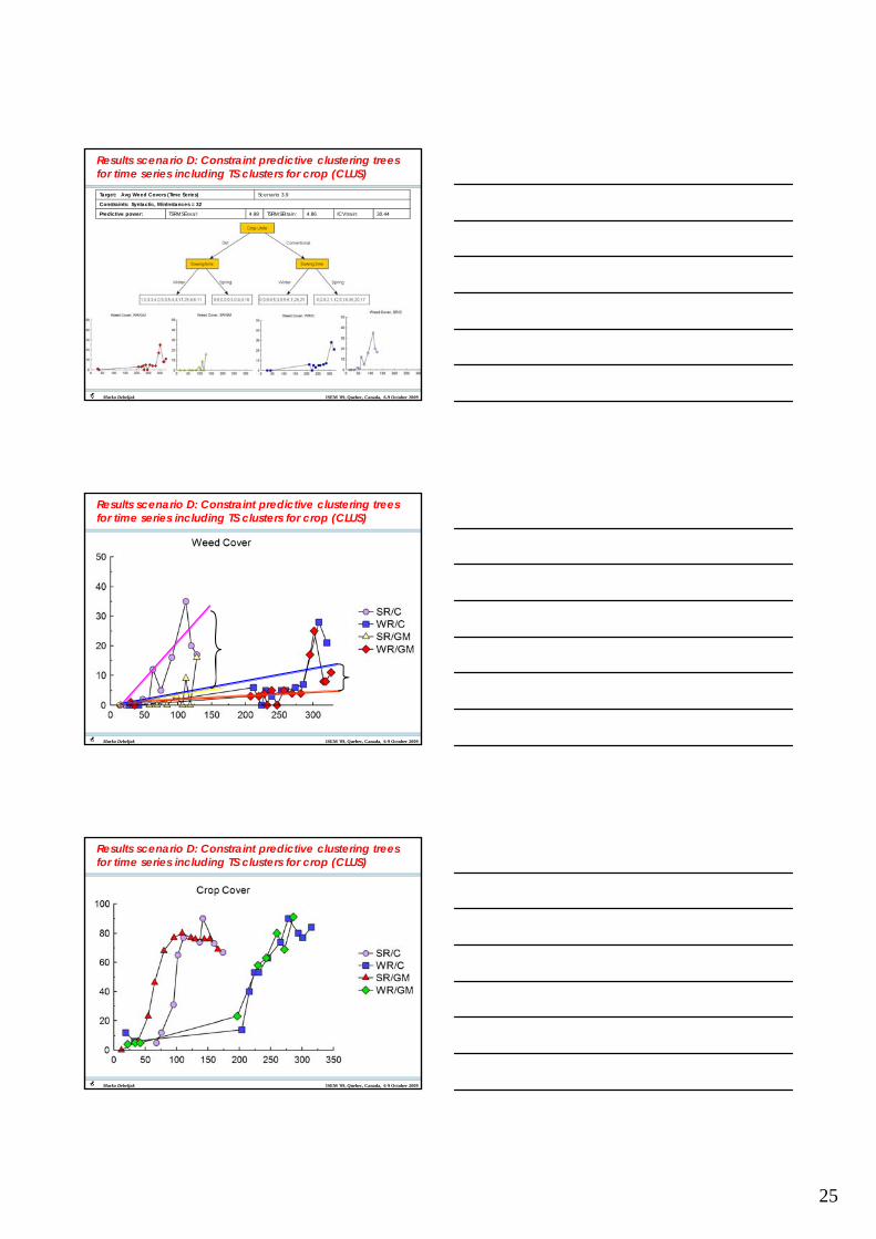
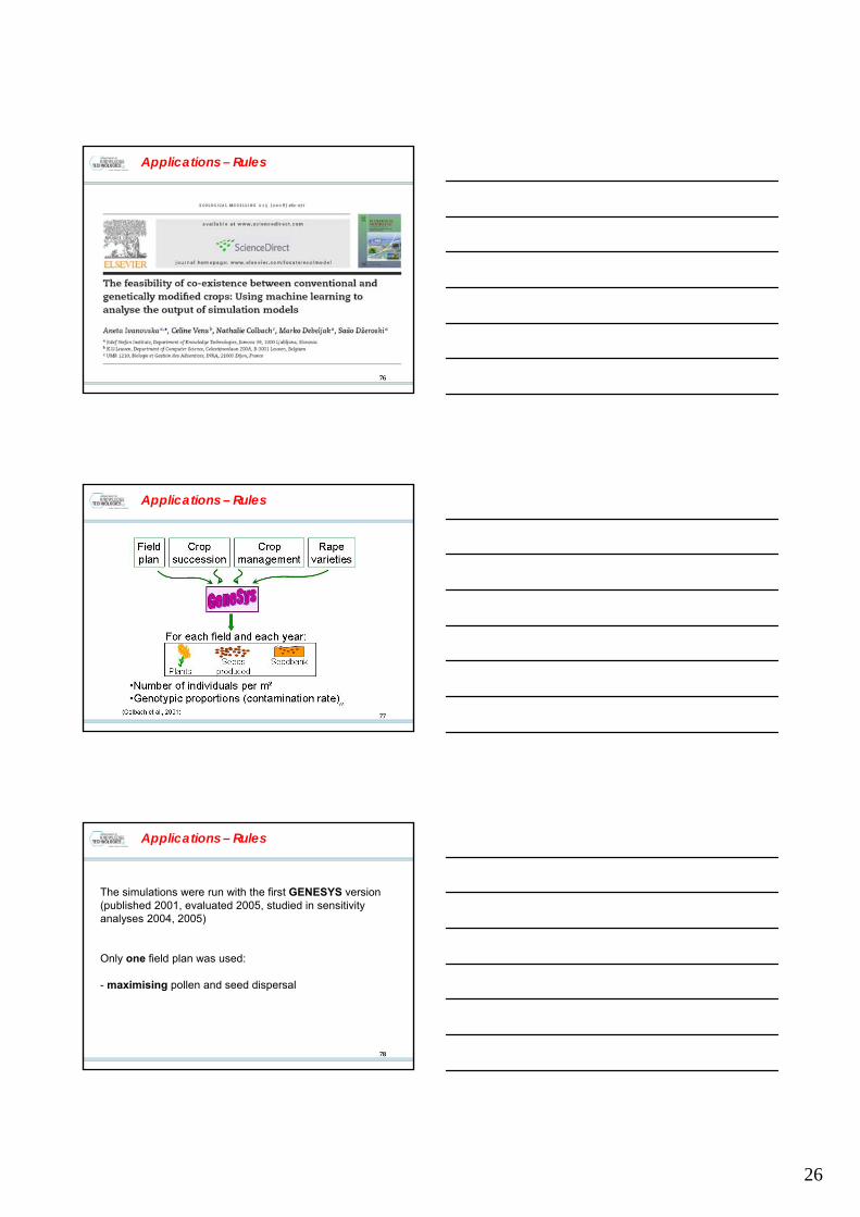
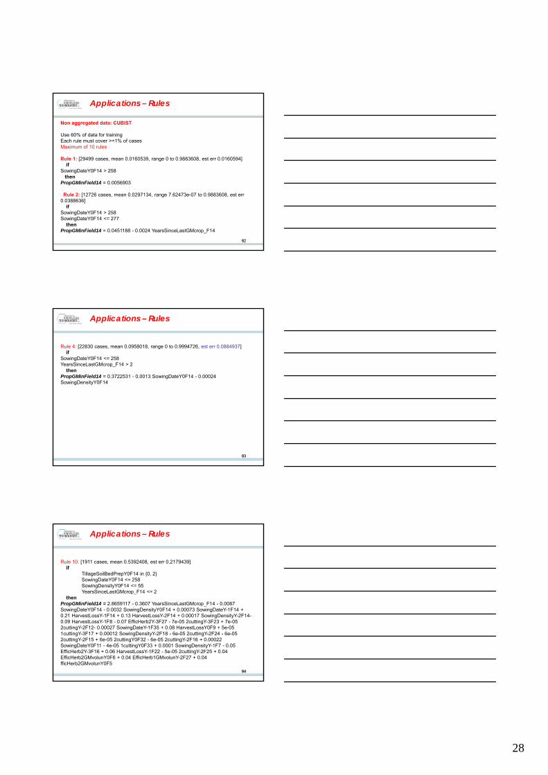
Results scenario D: Constraint predictive clustering trees for time series including TS clusters for crop (CLUS)
Results scenario D: Constraint predictive clustering trees for time series including TS clusters for crop (CLUS)
Marko Debeljak ISEM '09, Quebec, Canada, 6-9 October 2009
Results scenario D: Constraint predictive clustering trees for time series including TS clusters for crop (CLUS)
Marko Debeljak ISEM '09, Quebec, Canada, 6-9 October 2009
26
7676
Applications – Rules
7777
Applications – Rules
7878
Applications – Rules
The simulations were run with the first GENESYS version (published 2001, evaluated 2005, studied in sensitivity analyses 2004, 2005)
Only one field plan was used:
- maximising pollen and seed dispersal
27
7979
Applications – Rules
Large-risk field pattern
8080
Applications – Rules
Variables describing simulations
- simulation number- genetic variables- for each field (1 to 35), the cultivation techniques of year -3, -2, -1, 0- for each field (1 to 35) the number of years since the last GM oilseed rape crop- the number of years since the last non-GM oilseed rape crop
- proportion of GM seeds in non-GM oilseed rape of field 14 at year 0
-TOTAL NUMBER OF VARIABLES: 1899
8181
Applications – Rules
Run of experiment
• simulation started with an empty seed bank
• lasted 25 years,
• but only the last 4 years were kept in the files for data mining
• TOTAL NUMBER of simulations on the field pattern without the borders: 100 000
28
8282
Applications – Rules
Non aggregated data: CUBIST
Use 60% of data for trainingEach rule must cover >=1% of casesMaximum of 10 rules
Rule 1: [29499 cases, mean 0.0160539, range 0 to 0.9883608, est err 0.0160594]if
SowingDateY0F14 > 258then
PropGMinField14 = 0.0056903
Rule 2: [12726 cases, mean 0.0297134, range 7.62473e-07 to 0.9883608, est err 0.0388636]
Non aggregated data: CUBIST Options:Use 60% of data for trainingEach rule must cover >=1% of casesMaximum of 10 rules
Target attribute `PropGMinField14'
Evaluation on training data (60000 cases):Average |error| 0.0633466Relative |error| 0.47Correlation coefficient 0.77
Evaluation on test data (40000 cases):
Average |error| 0.0657057Relative |error| 0.49Correlation coefficient 0.75
8686
Conclusions
What can data mining do for you?
Knowledge discovered by analyzing data with DM techniques can help:
� Understand the domain studied
� Make predictions/classifications
� Support decision processes in environmental management
8787
Conclusions
What data mining cannot do for you?
� The law of information conservation (garbage-in-garbage-out)
� The knowledge we are seeking to discover has to come from the combination of data and background knowledge
� If we have very little data of very low quality and no background knowledge no form of data analysis will help
30
8888
Conclusions
Side-effects?
• Discovering problems with the data during analysis
– missing values
– erroneous values
– inappropriately measured variables
• Identifying new opportunities
– new problems to be addressed
– recommendations on what data to collect and how
89
1. Data preprocessing
DATA MINING – Hands-on exercises
90
DATA MINING – data preprocessing
DATA FORMAT• File extension .arff• This a plain text format, files should be edited by
editors such as Notepad, TextPad, WordPad (that do not add extra formatting information)
• File consists of – Title: @relation NameOfDataset– List of attributes: @attribute AttName AttType
• AttType can be ‘numeric’ or nominal list of categorical values, e.g., ‘{red, green, blue}’
– Data: @data (in a separate line), followed by the actual data in comma separated value (.csv) format
31
91
DATA MINING – data preprocessing
DATA FORMAT
@relation weather
@attribute outlook {sunny, overcast, rainy}@attribute temperature numeric@attribute humidity numeric@attribute windy {TRUE, FALSE}@attribute play {yes, no}
• Excel• Attributes (variables) in columns and cases in
lines
• Use decimal POINT and not decimal COMMA for numbers
• Save excel sheet as CSV file
93
DATA MINING – data preprocessing
• TextPad, Notepad
• Open CSV file
• Delete “ “ on the beginning of lines and save (just save, don’t change the format)
• Change all ; to ,
• Numbers must have decimal dot (.) and not decimal comma (,)
• Save file as CSV file (don't change format)
32
94
2. Data minig
DATA MINING – Hands-on exercises
95
DATA MINING – data preprocessing
• WEKA
• Open CVS file in WEKA
• Select algorithm and attributes
• Perform data mining
http://www.cs.waikato.ac.nz/ml/weka/index.html
96
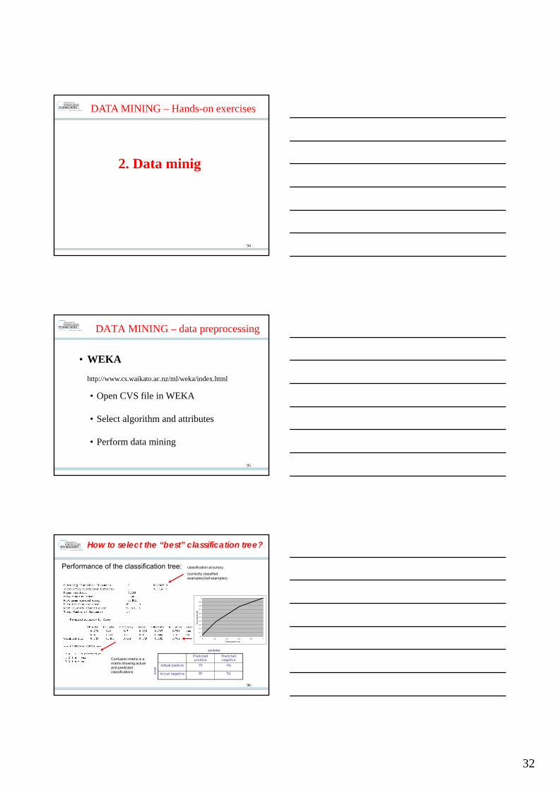
How to select the “best” classification tree?
Performance of the classification tree:
Confusion matrix is a matrix showing actual and predicted classifications
classification accuracy:
(correctly classified examples)/(all examples)
0
0.1
0.2
0.3
0.4
0.5
0.6
0.7
0.8
0.9
1
0 0.2 0.4 0.6 0.8 1
False positive rate
Tru
e p
osi
tive
rat
e
33
97
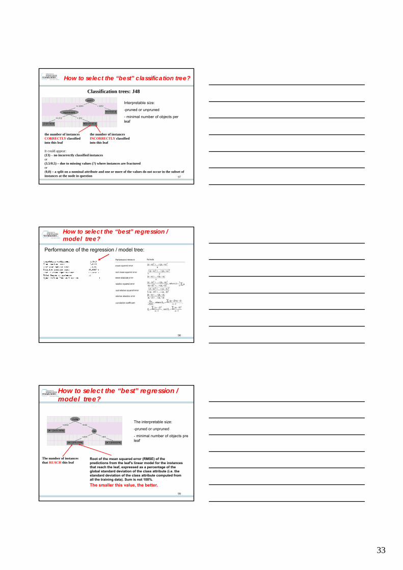
How to select the “best” classification tree?
Classification trees: J48
the number of instances CORRECTLY classified into this leaf
the number of instances INCORRECTLY classified into this leaf
It could appear:(13) – no incorrectly classified instancesor(3.5/0.5) – due to missing values (?) where instances are fracturedor(0,0) – a split on a nominal attribute and one or more of the values do not occur in the subset of instances at the node in question
Interpretable size:
-pruned or unpruned
- minimal number of objects per leaf
98
How to select the “best” regression / model tree?
Performance of the regression / model tree:
99
The number of instances that REACH this leaf
Root of the mean squared error (RMSE) of the predictions from the leaf's linear model for the instances that reach the leaf, expressed as a percentage of the global standard deviation of the class attribute (i.e. the standard deviation of the class attribute computed from all the training data). Sum is not 100%.
The smaller this value, the better.
How to select the “best” regression / model tree?
The interpretable size:
-pruned or unpruned
- minimal number of objects pre leaf
34
100
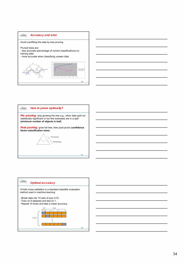
Accuracy and error
Avoid overfitting the data by tree pruning.
Pruned trees are:- less accurate (percentage of correct classifications) on training data- more accurate when classifying unseen data
101
How to prune optimally?
Pre-pruning: stop growing the tree e.g., when data split not statistically significant or too few examples are in a split (minimum number of objects in leaf)
Post-pruning: grow full tree, then post-prune (confidence factor-classification trees)
102
Optimal accuracy
10-fold cross-validation is a standard classifier evaluation method used in machine learning:
- Break data into 10 sets of size n/10. - Train on 9 datasets and test on 1. - Repeat 10 times and take a mean accuracy.