IV. Transport Phenomena

Lecture 18: Forced Convection in Fuel Cells II

MIT Student (and MZB)

As discussed in the previous lecture, we are interested in forcing fluid to flow in a fuel cell in order to increase the limiting current, and thus the power output of the device. The model problem considered has a steady uniform flow of fluid carrying the reactant at a constant concentration, c0, into a 2-D channel of height H. In this model we will assume that the fluid velocity profile across the channel is uniform (i.e. plug flow). We are interested in analyzing the transport of the reactant carried into the system by the convective fluid stream to the active membrane located at y = 0, which has a length of L.

y

Uniform Flow c = c0 δ(x)

Diffusion Layer

Wall

Membranec(y=0) = 0x = 0 x = L x

y = H

+ x = l1

Entrance Length x = l2

Figure 1: Model problem of forced convection in a fuel cell

From conservation of mass, there is a balance between convection and diffusion terms:

[1]

Since the flow is steady, the transient term can be neglected. In the region when x >> l1 , convection dominates over axial diffusion:

[2]

From scaling analysis, we can define l1 as the point where convection occurs at the same scale as axial diffusion. That is:

[3]

Nondimensionalizing the position variables as follows leads us to the Péclet Number, Pe. Let:

1

[4]

In the region where x >> l1 or , we can neglect axial diffusion and define a “time” variable t = x/U along the streamlines to obtain a 1D diffusion equation in terms of y only. This approach is valid because the fluid flow rate is invariant with location in our model. It is worth restating that the Péclet Number is a dimensionless value that represents the ratio of the rate of convection to the rate of diffusion in the system. We can redefine Equation [1] as:

[5]

and the “initial condition” at the inlet becomes: c(x = 0, y) = c(t = 0, y) = c0.

We are now ready to calculate the limiting current Ilim as a function of the fluid velocity, U, under the assumption that reactions are fast enough everywhere for c(t, y = 0) → 0 along the entire membrane when I→Ilim. The problem has now become:

y Wall y = H

c = c0

Membranec(y=0) = 0x = 0 x = L t = x/U

Figure 2: 1D diffusion model for forced convection in a fuel cell

Lecture 18: Forced convection in fuel cells (II) 10.626 (2011) Bazant

The limiting current is found by integrating the transverse mass flux along the membrane:

[6]

Below we will obtain an exact solution as a Fourier Series, but it is more accurate and easier when x or t to is small to find a boundary-layer similarity solution (as if H→∞) in the “entrance region”.

1. Entrance Region Using scaling analysis, the boundary layer thickness, δ(x), can be found:

[7]

Now we can define x = l2 to be the axial location where the boundary layer first spans the entire height of the channel, that is δ(l2) ~ H as is illustrated in Figure 1. Therefore:

2

[8]

For l1 << x << l2 , the boundary layer is much thinner than the channel height. Thus, we can set H = ∞. If we nondimensionalize l2 and δ :

[9]

we see that we need 1/Pe << << Pe in order to use the boundary layer approximation, which is only valid for small boundary layers, i.e. when Pe >> 1. With H = ∞ (i.e. the boundary layers are so thin compared to the channel height that we can solve using a semi-infinite channel instead of one with finite height), we have a similarity solution to the diffusion equation:

[10]

Note that here y/δ(x) is the “stretched” or “inner” coordinate of the boundary layer and that the error function, erf, is defined as:

[11]

Figure 3: Isoconcentration Lines for Entrance Region

Now that the concentration profile is known as a function of distance along the membrane, we can calculate the flux density, F, on the membrane:

[12]

From above, it is evident that the largest flux occurs near the inlet when x→0.

Lecture 18: Forced convection in fuel cells (II) 10.626 (2011) Bazant

3

Another dimensionless number that is commonly used is the Sherwood Number, Sh, which represents the ratio of convective to diffusive mass transport. Here it is a dimensionless flux:

[13]

2. Fully Developed Region For x > l2 or = O(Pe), we can still neglect axial diffusion, however we must solve the full problem for a finite channel height, H. First, let us define more dimensionless variables:

[14]

We can now redefine the diffusion problem as:

[15]

with initial condition: , and boundary conditions: and . This

problem can be solved with Fourier Series, or more generally by “Finite Fourier Transform”1, as a general series expansion in separable solutions to the PDE:

is the transform (“FFT”) and

[16]

where are the basis functions, determined by the following general procedure. The series expansion is needed since the boundary conditions are inconsistent with a single separable solution.

2.1 Step 1 - Determine the Basis Functions Generally, to solve we want the basis functions, , to be eigenfuctions of the

linear operator :

[17]

and satisfy the homogeneous boundary conditions:

[18]

1 See W. M. Deen, Analysis of Transport Phenomena.

Lecture 18: Forced convection in fuel cells (II) 10.626 (2011) Bazant

4

After applying the BC’s it is seen that: Bn = 0 and λn = (n+½)π. Therefore, we have the series:

[19]

This method is most useful if this set of functions satisfy the definition of orthogonality, which is a generalization of perpendicular vectors to infinite dimensions. Two functions ϕn and ϕm are said to be orthogonal if:

0, m ≠ n ϕn ,

1 ⎧⎪ϕm = ϕ y ( n )d y [20]∫ ( )ϕm y = δm = ,n ⎨0 ⎪ 1, m = ⎩ n

Furthermore, we choose An so that , which makes the set orthonormal.

A crucial property of our linear operator L (including its boundary conditions) is that it is self-adjoint , meaning that ϕ1, Lϕ2 = , since this implies that the its eigenfunctions are orthogonal2

Lϕ1,ϕ2

It is then found that:

[21]

2.2 Step 2 - Transform the PDE into an ODE Now let’s substitute our assumed solution, Equation [16], into the PDE of Equation [15]:

[22]

A property of eigenfunctions is that both sides of the PDE must be equal to .

(We are essentially performing separation of variables and setting both sides equal to the same constant, but we can only do it for each term involving a single basis function). Now that the basis functions are orthogonal, the coefficients must be equal:

2 More generally, all Strum-Liouville differential operators of the form 1

Lu d ⎛ du ⎞

= − p(x) + q(x)u(x) with homogeneous Robin boundary conditionsw(x) dx ⎟ dx ⎜ ⎝ ⎠

u + adu = 0 are self adjoint with respect to the inner product, ϕ1,ϕ2 = ∫ϕ1(x)ϕ2 (x)w(x)dx , sodx

the eigenfunctions of such operators (which come up often in convection-diffusion problems, e.g. Bessel functions in cylindrical coordinates) are automatically orthogonal and convenient for series expansions.

Lecture 18: Forced convection in fuel cells (II) 10.626 (2011) Bazant

5

[23]

which yields the solution:

[24]

2.3 Step 3 – Evaluate the Constants Using Initial and Boundary Conditions Because , we have:

[25]

To invert the transform, take the inner product with ϕm:

[26]

Using orthonormality:

[27]

Now that the coefficients have been determined, we can put it all together to form the solution:

[28]

Figure 4: Isoconcentration Lines for Fully Developed Flow Region For >> 1 (or x >> l2) in the fully developed region, the first term in the series dominates:

Lecture 18: Forced convection in fuel cells (II) 10.626 (2011) Bazant

6

[29]

And the flux is:

[30]

Finally, we can calculate the limiting current, Ilim, by integrating the mass flux over the membrane:

[31]

where .

The fuel utilization, γlim, is defined as the ratio of the fuel consumed to the fuel input into the fuel cell:

[32]

and γlim are related by:

[33]

At a given fuel utilization we can boost the limiting current and thus the power, P = IV, by having fast flow (Pe >> 1) and thick channels, which allow more fuel into the system.

2.4 Flow Regimes Let’s examine the limiting current and fuel utilization in two flow regimes:

2.4.1 Fast Flow (l2 >> L) In this regime the fluid is moving quickly, which means the boundary layer is thin compared to the channel height. This is equivalent to saying that l2 is located beyond the axial extent of the membrane (0 < x <L).

Lecture 18: Forced convection in fuel cells (II) 10.626 (2011) Bazant

x = 0 x = L

Uniform Flow c = c0 δ(x)<<H

y

x

y = H

7

Figure 5: Fast Flow Regime for a Fuel Cell

If δ(x) << H, then DL/U << H2 and (D/UL)(L/H)2 << 1 → Pe(H/L)2 >> 1. From Equation [13]:

[34]

Therefore, the fuel utilization in this regime is:

Because the quantity

[35]

is constant in Equation [35], it is obvious that in the fast flow regime there is an inherent tradeoff between power and fuel utilization. That is, although faster flows generate larger power due to an increased Ilim, less of the fuel is able to diffuse to the membrane by the time it reaches an axial position of x=L.

2.4.2 Slow Flow (l2 << L) In this regime the diffusion profile is fully developed and the boundary layer has reached the top of the channel for much of the length of the membrane.

Lecture 18: Forced convection in fuel cells (II) 10.626 (2011) Bazant

Figure 6: Slow Flow Regime for a Fuel Cell

Uniform Flow c = c0

δ(x)

x = L x

y = H

x = 0 x = l2

Now,

When , Equation [34] becomes .

[36]

The fuel utilization in this case is:

[37]

Therefore, for slow flow or long channels, all of the fuel is consumed, but the power is low.

Note that by keeping only the first term in the Fourier series for the slow flow we found that

y

8

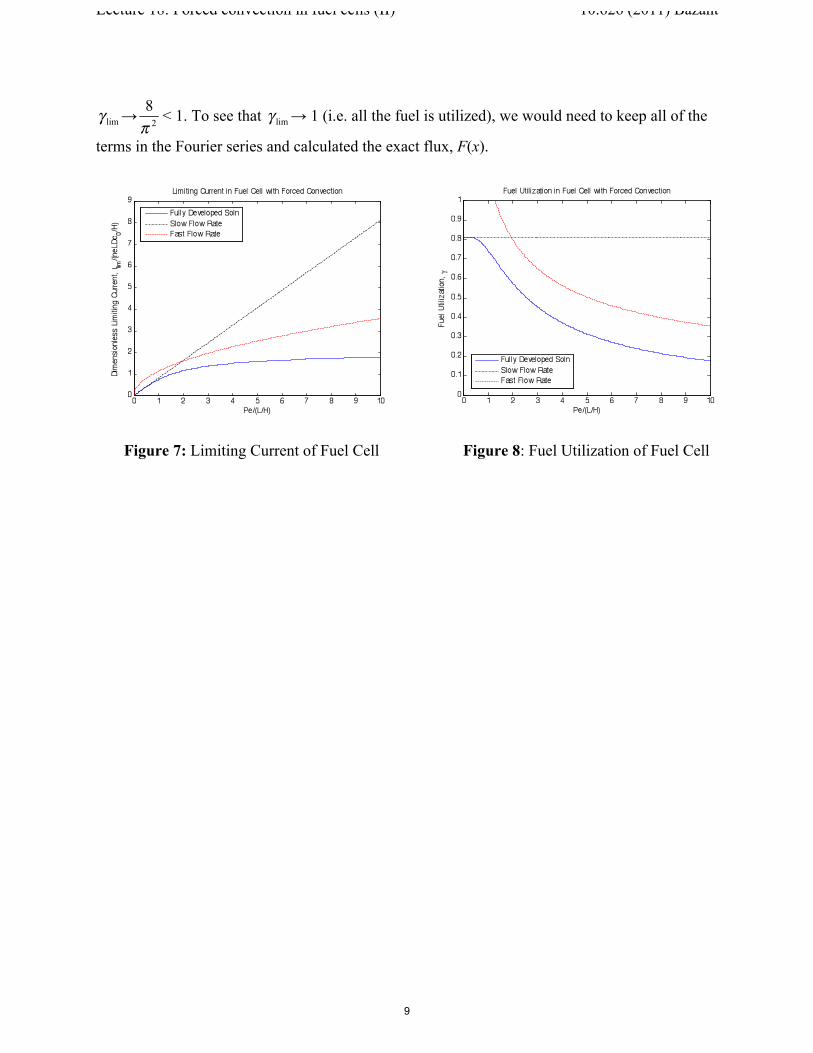
Figure 7: Limiting Current of Fuel Cell Figure 8: Fuel Utilization of Fuel Cell

Lecture 18: Forced convection in fuel cells (II) 10.626 (2011) Bazant

→ < 1. To see that → 1 (i.e. all the fuel is utilized), we would need to keep all of the

terms in the Fourier series and calculated the exact flux, F(x).

9

MIT OpenCourseWarehttp://ocw.mit.edu

10.626 Electrochemical Energy SystemsSpring 2014

For information about citing these materials or our Terms of Use, visit: http://ocw.mit.edu/terms.