IZA DP No. 630 State Dependence in Unemployment Incidence: Evidence for British Men Revisited Wiji Arulampalam DISCUSSION PAPER SERIES Forschungsinstitut zur Zukunft der Arbeit Institute for the Study of Labor November 2002
Transcript
IZA DP No. 630
State Dependence in Unemployment Incidence:Evidence for British Men Revisited
Wiji Arulampalam
DI
SC
US
SI
ON
PA
PE
R S
ER
IE
S
Forschungsinstitutzur Zukunft der ArbeitInstitute for the Studyof Labor
November 2002
State Dependence in Unemployment Incidence:
Evidence for British Men Revisited
Wiji Arulampalam University of Warwick and IZA Bonn
This Discussion Paper is issued within the framework of IZA’s research area Welfare State and Labor Market. Any opinions expressed here are those of the author(s) and not those of the institute. Research disseminated by IZA may include views on policy, but the institute itself takes no institutional policy positions. The Institute for the Study of Labor (IZA) in Bonn is a local and virtual international research center and a place of communication between science, politics and business. IZA is an independent, nonprofit limited liability company (Gesellschaft mit beschränkter Haftung) supported by the Deutsche Post AG. The center is associated with the University of Bonn and offers a stimulating research environment through its research networks, research support, and visitors and doctoral programs. IZA engages in (i) original and internationally competitive research in all fields of labor economics, (ii) development of policy concepts, and (iii) dissemination of research results and concepts to the interested public. The current research program deals with (1) mobility and flexibility of labor, (2) internationalization of labor markets, (3) welfare state and labor market, (4) labor markets in transition countries, (5) the future of labor, (6) evaluation of labor market policies and projects and (7) general labor economics. IZA Discussion Papers often represent preliminary work and are circulated to encourage discussion. Citation of such a paper should account for its provisional character. A revised version may be available on the IZA website (www.iza.org) or directly from the author.
State Dependence in Unemployment Incidence: Evidence for British Men Revisited�
The issues of persistence in the observed labour market status of men are investigated using the British Household Panel Survey for the period 1991-97. The paper extends previous work in many directions. In particular, problems of endogenous initial conditions, and unobserved heterogeneity, are addressed within the context of different definitions of unemployment. In addition, allowance is also made to accommodate the ‘stayer’ phenomenon in the state of employment. All these were found to be very important in the estimation of the effect of scarring. JEL Classification: C15, C23, C25, J64 Keywords: dynamic binary panel models, unemployment, state dependence, unobserved
heterogeneity, initial conditions Corresponding author: Wiji Arulampalam Department of Economics University of Warwick Coventry CV4 7AL United Kingdom Tel.: +44 (0)24 7652 3471 Fax: +44 (0)24 7652 3032 Email: [email protected]
� The BHPS data used in this paper were collected by the ESRC Research Centre on Micro-Social Change at the University of Essex and made available through the ESRC Data Archive. I should like to thank Mark Taylor for providing help with the creation of some of the variables used in the study and to the Institute for Social and Economic Research Centre for providing the data on Travel-To-Work-Area unemployment and vacancy rates. I should also like to thank Alison Booth, Norman Ireland, Robin Naylor, Mark Stewart, Mark Taylor, and participants at the 8th International Conference on Panel Data held in Gotenborg in June 1998, and the Royal Economic Society Conference held in St. Andrews, Scotland in July 2000, for useful comments. This paper was produced as part of the project on Unemployment and Technical and Structural Change, which was funded by the Leverhulme Trust. The views in the paper are those of the author, and do not necessarily reflect those of the Leverhulme Trust. This paper is a revised version of ‘State dependence in unemployment incidence: evidence for British men 1991-95’ (1998). Any errors remain my responsibility.
The extent to which a previous unemployment experience increases the probability of an
individual being unemployed in the future has important implications for labour market
policies. Repeat incidences of unemployment can also lead to considerable poverty, social
exclusion and distress.1 If there is considerable persistence, short run policies such as job
creation schemes and wage subsidies to employers, may be used to alter the equilibrium
unemployment rate. Hence, not only an early successful intervention is required but the
identification of the correct target groups also becomes necessary.
A recent response of the Government has been the introduction of the ‘New Deal’
program in 1998. One of the main aims of this program is to provide incentives to
unemployed individuals on benefits to move to employment. Impositions of tighter
conditions on benefit eligibility and job search are important parts of this program. But
targeting such policies using very strict definition of ‘unemployment’ ignores a large group of
unemployed individuals who may not satisfy these strict criteria but are also affected by
repeat incidences of unemployment. This paper addresses the issue of persistence using
different definitions of unemployment using longitudinal data on a group of men over the
period 1991 to 1997 from the British Household Panel Survey (BHPS).2 This is the same
dataset that was used in Arulampalam, Booth, and Taylor (2000) (henceforth called ABT)
1 Arulampalam (2001) finds that there is a wage loss associated with post-unemployment job. Stewart (2002)
finds that individuals who are unemployed go back to low-pay jobs, thus leading to additional income and welfare losses. Clark and Oswald (1994) find that unemployment causes a lot of distress and being unemployed is one of the most important causes of unhappiness.
2 The cut-off of 1997 was used in order to avoid complications with regard to ‘persistence’ measure, arising from the introduction of the ‘New Deal’ program in 1998, which was aimed at individuals who had been unemployed for six months or more.
4
although a shorter time period was used in ABT. This paper extends the work of ABT and
others in several ways.
First extension concerns the definition of ‘unemployment’ used in the analysis. One
of the most commonly used definitions of unemployment is unemployment with search. For
example, one popular definition is that of the International Labour Organisation (ILO). Under
this definition an individual is classified as being unemployed if (i) the individual does not
have a job; (ii) s/he has searched for a job in the past four weeks; and (iii) s/he is available to
start work immediately. This is the definition used by ABT. But sometimes researchers
restrict the period of search to one week. But not all individuals who claim to be unemployed
in the sample satisfy the search or the availability to start work criteria. Some of the
individuals who do not satisfy these criteria are found to be in employment later on in the
sample.3 Looking at persistence in terms of a stricter definition of search unemployment may
therefore be of little value for some policy purposes. For example, if one needs to look at the
effect of wage pressures coming via possible increases to labour supply from these
individuals who do not satisfy the standard search criterion, it is important to work with this
group of individuals included in the analysis.
Another reason for looking at the impact of using different definitions for
‘unemployment’ is that most of the studies that look at persistence commonly use a two-state
model of the labour market because of lack of observations to enable one to specify and
estimate a general multi-state model.4 Since a dynamic model of this type requires individuals
to have continuous observations, an inevitable outcome of using a stricter definition of
3 Gregg and Wadsworh (1998) find that “those excluded from unemployment because they are not available to
start in two weeks but are searching for work are more likely to enter employment than the long term unemployed. The data set used was the British Labour Force Survey for the period 1981 to 1997.
4 Few examples of studies that have looked at the issue of persistence in unemployment are, Narendranathan, et al (1985), Flaig et al (1993), Muhleisen and Zimmermann (1994), Narendranathan and Elias (1995), McCulloch and Dex (1996) and, Arulampalam et al (2000).
5
‘unemployment’ is to discard individuals who do not satisfy the criteria. This may potentially
bias the estimated effects of persistence. This study therefore looks at the issue of persistence
using different classifications of the variable of interest. These are (i) self reported
unemployment where no search criterion is used, (ii) search unemployment where the search
period is four weeks (ILO definition), and (iii) search unemployment where the search period
is one week.5 These are important distinctions that result in various degrees of attrition in the
sample used for the analysis with the last classification being the one with the least attrition.
Second extension of this work concerns the issue of endogeneity of ‘initial
conditions’. The initial conditions problem arises when the start of the observation period
does not coincide with the start of the stochastic process generating individuals’
unemployment experiences. An individual who is observed in the state of unemployment at
the start of the observation period may be there because of an earlier history of unemployment
(state dependence) or because of some unobserved characteristic affecting the job-offer or job
retention rates facing that individual. In order to unravel these two effects, the initial
condition needs to be explicitly modelled rather than assumed exogenously given. ABT used
a two-step technique proposed by Orme (1997) to address this problem. This technique is
only valid if the problem caused by ‘endogeneity’ of the initial conditions is not severe. The
model for the ‘initial’ observation is explicitly specified and estimated in this paper.
Third extension concerns the specification of the distribution of the unobservables.
The usual assumption of normally distributed unobservables is extended to accommodate the
fact that there are many individuals who never experience a spell of unemployment. As
shown below, the estimated magnitude of the persistence effect is indeed sensitive to this.
5 Because of small cell sizes, the analyses presented in this paper are conducted in a two-state model instead of
a multi-state model of the labour market.
6
The model estimated in this paper allows for this by allowing for empirically determined
masses at the two extremes, i.e. plus and minus infinity of the Normal mixing distribution.
The remainder of this paper is set out as follows. Section II presents the dynamic
panel data model and discusses the various estimation issues. Section III discusses the data
and the sample used. The estimates of ‘scarring’ are presented and discussed in Section IV.
Final section summarises and concludes.
II MODEL AND ESTIMATION
II.1 Background
The extent to which a previous unemployment experience increases the probability of an
individual being unemployed in the future has important implications for labour market
policies. An individual may be stigmatised by long or repeated spells of unemployment that
are beyond his control. Prospective employers may use the experience of unemployment as a
signal of ‘unemployability’. It may also result in depreciation of acquired human capital.
Hence he may receive fewer or no job offers the longer is his experience of unemployment or
the greater the number of spells.
Of course, an unemployed individual may also become less choosy as unemployment
spell lengthens. Consequently, he may revise downwards his reservation wage, and accept a
poor quality job that is not expected to last long. For this reason, men who have experienced
unemployment in one period may be more likely to be unemployed subsequently. While this
study is unable to distinguish between these various competing hypotheses as to the causes of
state dependence because of the reduced form nature of the model estimated, it is able to
establish empirically whether genuine state dependence exists in this sample.
Consider the state of unemployment. The proportion of time spent by an individual in
unemployment will depend on the probabilities of entry into and then exit from the state of
7
unemployment. This requires some theory of labour turnover as a framework for the analysis.
Since the study is concerned with reduced form models of unemployment incidence, only a
few salient remarks are presented instead of a detailed discussion of various theories of labour
turnover. First consider the determinants of the probability of entry into unemployment.
In a world where there are only two states, employment and unemployment, an
individual can enter unemployment either voluntarily or involuntarily. An individual will
quit a job and enter unemployment if the value of outside prospects including the expected
spell of unemployment exceeds the expected earnings in the current job. On the other hand,
the probability of involuntary separation will depend on the individual’s productivity relative
to the wage.
As far as the determinants of the probability of exit out of unemployment is
concerned, this will depend on the arrival rate of acceptable job offers which in turn will
depend on how the individual searches for a suitable job and how the prospective employer
views the individual as a suitable candidate.
Hence, the usual set of control variables such as demographic and family variables,
level of education, and variables to proxy labour market tightness are included in the reduced
form model of unemployment incidence. These variables reflect individual search intensity,
and job-offer arrival or job-retention rates.
Not only observable but unobservable individual characteristics may also affect the
propensity of certain individuals to be unemployed. Individuals may have undesirable
attributes such as lack of motivation that, while unobservable to the statistician, may be used
by employers to affect the rates of job-offers and job- retentions. A proper control of this is
necessary in order to avoid biasing the estimated state dependence effect in the model of
unemployment incidence.
8
II.2 The Econometric Model
The observed dependent variable is binary, taking the value of one if the individual is
unemployed at the time of the interview, and zero otherwise. This variable is observed, in the
sample, at most seven consecutive separate interview dates. The model for individual i at the
yit* = xit’ββββ=+ γyit-1 + αi + uit i=1,....,n and t=2,..,Ti (1)
Note, in the above model, variance(uit) = σ2u for t=2,..,Ti and variance(ui1) =
σ ρη2 21( )− . As shown in Heckman (1981a, 1981b), under the additional assumption that αi
10
and uit are jointly multi-variate normal, this model can be easily estimated by noting that the
distribution of yit* conditional on αi, xit and yit-1, is independent normal. Marginalising the
likelihood with respect to the α gives the likelihood function for individual i,
{ ])1(2 ) [( Lu
uu2t
−ασσ
+σγ
=+σ
Φ= α∞
∞− =∏ it1-itit
T
i y~y' =
==
=
βx
} d )( )]1(2 ) 11
[(22
ααφ−αρ−
ρ+ρ−σ
λΦη
~~y~' i1iz (5)
where ~α i = αi / σα and, φ= and Φ are the density and the distribution function of the standard
normal variate.
A normalisation is required next because of the binary nature of the variable under
study. A convenient normalisation is that the variance of the error term uit = 1 for all
t.==Equation (5), thus becomes,
( ])1(2 ) [( L 2t
−ασ+γ=+Φ= α
∞
∞− =∏ it1-itit
T
i y~y' =
==
=βx
) ααφ−ασθ+Φ α~~y~' i1i d )( )]1(2 ) [( λz (6)
An obvious weakness in the above specification is the assumption of normally
distributed unobserved heterogeneity. This assumption does not allow enough flexibility to
model the phenomenon that some individuals are always observed to be in the same state in
the sample (Narendranathan and Elias (1982)). A very large positive (negative) value for the
unobservable α=will give a very large (small) value for y* and hence a very large (small)
probability of being in unemployment. This is accommodated by allowing for empirically
determined masses at the two extremes, i.e. plus and minus infinity of the Normal mixing
distribution. This gives the following likelihood for individual i,
11
1010
1
10
0*
1L
1)-(1
1L
ψ+ψ++
���
�
ψ+ψ+ψ+�
���
�
ψ+ψ+ψ= ∏∏
==
iT
1tit
T
1titi
ii
yy (7)
where, Li is given by equation (6) and ψ0=and ψ1 are the unknown end point parameters.
Hence, the proportion of individuals who are assumed to have a very large or a very small
unobserved component are given by p0 and p1, where,
10
00 1
pψ+ψ+
ψ= and
10
11 1
pψ+ψ+
ψ= respectively. (8)
Some testable restrictions on the Model
1. Exogeneity of the Initial Condition: θ=0 in (4) is a test of this hypothesis that the initial
conditions can be treated as exogenous. Also note, under the assumption that the initial
condition is exogenous, the above model reduces to a simple random effects probit model
over t=2,...,Ti.
2. Unemployment process observed from the beginning: This is equivalent to a test of θ=1 in
(4). This model can be estimated simply by creating a time dummy (dum) which equals one
in t=1 and zero otherwise. Equations (4) and (1) together now become
( )[ ] ( ) ( )y dum dum y dum uit*
it it 1 i i it' '= ∗ − + − + ∗ + +−x z1 1 ββββ λλλλγ α (9)
Equation (11) can then be estimated using all seven years of data with standard software
packages, which allow estimation of random effects probit models.
12
3. No unobservable time invariant individual characteristics:
Note corr(vit,vis)=corr(αi+uit ,αi+uis)=σ
σ σα
α
2
2 2+ u
= r say, for all t=≠ s≠ 1. (10)
Hence, a test of H0 : σα2=0 (which is a test that there are no unobservable characteristics in
the sample and therefore the model collapses to a simple probit7) is equivalent to a test of H0:
r=0 in equation (10). This can be tested as a likelihood ratio test but the test statistic will not
be a standard chi-sq test since the parameter restriction is on the boundary of the parameter
space. The standard likelihood ratio test statistic has a probability mass of 0.5 at zero and 0.5
χ2(1) for positive values. Thus a one-sided 5% significance level test requires the use of the
10% critical value (Lawless (1987)).
Interpretation of γγγγ.
A convenient way to interpret the estimated persistence effect γ is required. One such method
is to look at the change in the predicted probabilities conditional on previous labour market
status. This is the one provided in Chamberlain (1984). This is the standard marginal effect
calculation in qualitative dependent variable models but accounts for the distribution of
unobserved heterogeneity in the population. For each individual, predicted probabilities are
calculated conditional, first on unemployment in the previous period and secondly on
employment in the previous period. The difference between the first and the second averaged
over the sample gives an estimate of state dependence or the persistence effect. This is the
7 Comparisons of ordinary probit results with those from a random effects probit model need to account for
different normalisations used by commercially available software (Arulampalam (1999)).
13
probability of observing a randomly chosen individual in unemployment in the current period
conditional on previous labour market status.
In addition to the above measure of ‘scarring’, the ratio of the two conditional
probabilities is also reported. This would tells us how large the conditional probability of
being in unemployment this period conditional on previous unemployment relative to
previous employment. As seen below, both measures are informative.
III THE DATA AND THE SAMPLE
The data are from the first seven waves of the British Household Panel Survey (BHPS), a
nationally representative survey of households randomly selected south of the Caledonian
Canal.8,9 The first wave of the BHPS was conducted from September to December 1991, and
annually thereafter (see Taylor (1996) for details). The sample used includes (i) all men who
were interviewed in 1991 (the first wave)10, (ii) aged 16 or over and under 55 at the initial
wave, and (iii) had a non-missing labour market status and not in full-time education. Since
the nature of the problem being analysed (lagged dependent variable is a regressor) requires
one to have consecutive information on labour market, the sample was further restricted to
only include men until they missed a direct interview. Then men were also required to be
active in the labour market continuously to be included in the sample. The number of eligible
sample members in each wave for this sample of 3024 men is provided in Table 1 Column
[1].
8 Thus the north of Scotland is excluded. 9 Also see footnote 2. 10 About 4% of the sample was lost because of either giving a proxy-interview or a telephone interview at each
wave. Only direct interview sample were selected because of missing values for many variables of interest for individuals who did not give a direct interview.
14
Of the original 3024 men, 15.3% of men did not appear in 1992 wave, and a further
10% of the original sample was not in by the 1993 wave. By the end of the sample period,
only 61% of the sample members had been present in all seven waves after applying the
selection criteria as outlined above. Column [2] to [4] lists the number of individuals who
contributed in each wave to the various analyses conducted. The two labour market statuses
considered are, (i) employment including self-employment, and (ii) unemployment. The least
restrictive assumption in terms of the definition used for the dependent variable is
‘unemployment’ and information for this is provided in Column [2]. Column [3] uses the
standard ILO definition and thus excludes all those in Column [2] who said that they have not
searched in the last four weeks. This is the classification of ‘unemployment’ that was used by
ABT. Column [4] restricts the sample further to only consider individuals who had been
searching in the past one week.
Looking across the columns of Table 1, it is interesting to note that the rate of attrition
over waves is very similar across various definitions used in the analyses. From the start to
the end year, approximately 40 to 45% of the original sample members are lost. The largest
loss was from wave 1 to wave 2. About 18% of wave 1 men did not appear in wave 2
sample. Approximately another 10% did not appear in wave 3 sample. But rate of attrition
has been less than 5% per wave since then. This rate of attrition is also remarkably close to
the original ‘interview’ sample attrition that required the individuals to be present at
consecutive interviews (plus other selections as discussed above).
Table 2 gives some information about the distribution of unemployment spells across
waves for all men with valid data for variables used in the analysis. The average rate of
unemployment over this seven-year period was 6.8%. Restricting the sample to those who
satisfy the ILO definition of unemployment, the average rate of unemployment goes down to
4.8%. Applying a very strict definition of search over the last week reduces this even further
15
to 4%. Thus, the average unemployment rate amongst our sample members over this period
is about 40% more than the average rate of ‘search unemployment’ in the sample.
Unemployment rates are found to decline during the sample period with the first decline
taking place in 1992 and another one in 1994.
Table 2 also gives the raw data conditional probabilities. There is a lot of persistence
over this period as measured by the probability of being in ‘unemployment’ at the time of
interview in a year given the same status in the previous interview period. The state
dependence for the case of ‘unemployment’ is about 56 percentage points over the sample
period with the probability of being in unemployment for an individual with previous
unemployment (at last year’s interview period) is 22 times higher compared to someone
without this previous unemployment. Restricting the sample by imposing search criterion
reduces the scarring effect to about 51 to 47 percentage points depending on how one defines
search, and also increases the differential effect. The reason for this is that as one imposes the
search criterion, the probability of unemployment for a previously unemployed individual
decreases, but at the same time, this probability for a previously employed individual
decreases by a larger amount.
The most interesting observation that emerges from this table is the fact that although
the aggregate unemployment rate had been coming down over this period, the scarring effect
as measured as the differences in the two conditional probabilities has not changed much.
But what has happened is that the unemployment incidence among the previously employed
people has been going down at a faster rate compared to previously unemployed people.
The interesting question is how much of the observed persistence in the raw data is
due to observed characteristics, unobserved characteristics, and genuine state dependence.
This is addressed through the multivariate analysis presented next.
16
IV. EMPIRICAL RESULTS
The models estimated are reduced form models of ‘unemployment’ incidences where three
different definitions of the state of ‘unemployment’ are considered. These are, (i)
unemployment with and without search, (ii) unemployment with search over the last four
weeks (ILO definition), and (iii) unemployment with search over the past one-week. The last
of these is the most restrictive definition with the first being the least restrictive.
The models include, as discussed previously, the usual set of control variables such as
demographic and family variables, level of education, and variables to proxy labour market
tightness. These variables reflect individual search intensity, job-offer arrival and job
retention rates. The persistence effect is accounted for by the inclusion of the previous labour
market status variable along with observable characteristics and, with the allowance for
unobservable individual characteristics in the model.
The analysis presented does not enable one to distinguish between these various
competing hypotheses as to the causes of state dependence. But it does allow one to establish
empirically, whether state dependence exists in the sample used and to investigate the
sensitivity of the results to different definitions of ‘unemployment’ used.
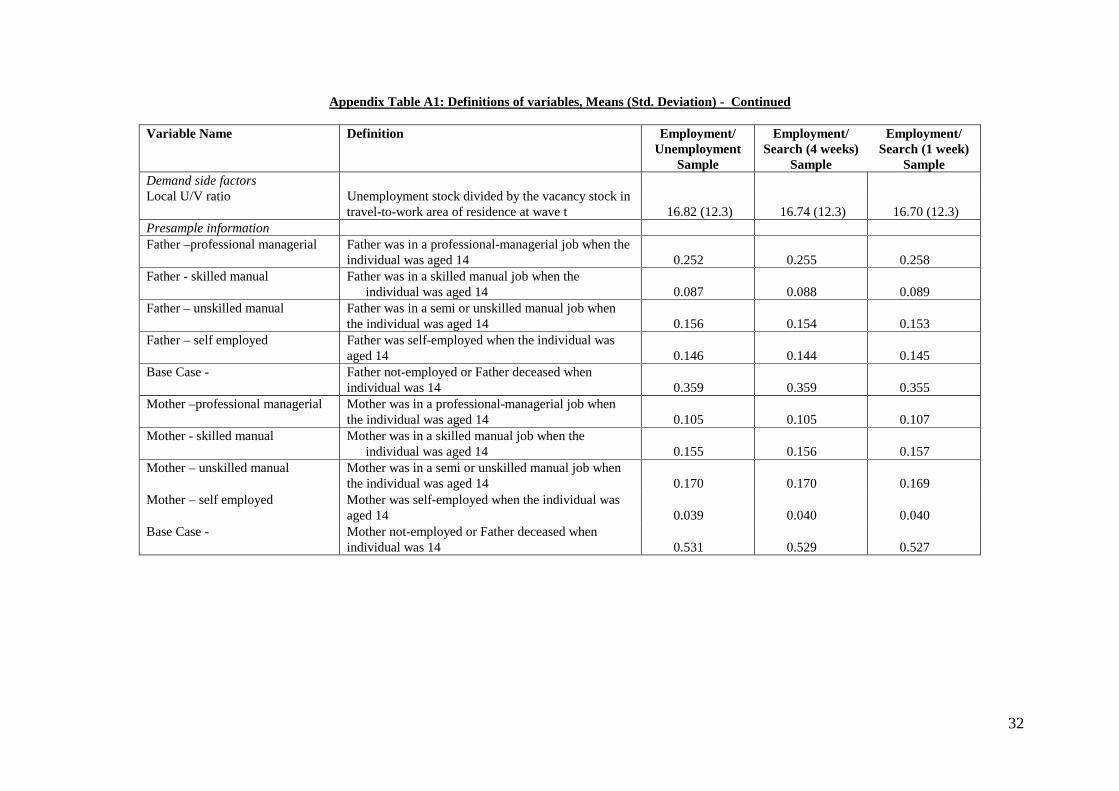
Definitions of the explanatory variables and the respective sample means are shown in
Appendix Table A1. All the variables that come under the heading of ‘Pre-sample
Information’ are the variables that were used to identify the initial condition model. Not
surprisingly, as one starts to impose various search criterion restrictions on the selection, there
are: (i) fewer local authority renters; (ii) more owner-occupiers with mortgage; (iii) fewer
men with health problems and disability; (iv) more men with a degree or higher, and (v)
fewer men with no qualifications.
Given the growing concern among the policy makers over the deteriorating labour
market positions of lower educated young people, in all the models estimated, the persistence
17
effect was allowed to vary with age as well as qualifications in a very broad manner. One
distinction is those men who are under 25 years of age (the age for eligibility for the ‘New
Deal’ program) from those who are older than 25 and the other is those who have at least an
‘O’ Level qualification level (obtained at or around the minimum school-leaving age) from
those who do not have.11
Before the discussion of the results, an important issue needs to be addressed. In the
data used, successive interviews were carried out approximately one year apart. One possible
concern that may arise with respect to the interpretation of the estimated persistence effects is
to do with the possibility that the persistence effects that are estimated are picking up the
effects coming via one continuous spell of unemployment instead of being two separate
unemployment spells. It is therefore important to bear in mind the following. First, since
unemployment is treated as a random variable, however far apart the consecutive
observations are, one would always find some individuals to be in a continuous spell of
unemployment. As long as the average unemployment duration is less than the time interval
between two successive interviews, on average, one would expect most of the individuals
who are observed to be in unemployment at two consecutive interviews, to be in two different
spells and therefore not drive the results one obtains.12 Second, although for some policy
purposes it is important to find out whether an individual is experiencing a very long spell of
unemployment or just very short duration repeat spells, both cases should be of concern to
policy makers because of the associated welfare costs associated with unemployment. A
11 The education variable was originally measured by four dummy variables, indicating the highest qualification
attained by the individual by 1991. These variables were Degree (a university degree), Other-higher (other higher qualification equivalent to a degree), A-level (one or more advanced-level qualifications representing university entrance-level qualifications usually taken at or around the age of 18) and, O-level (one or more ordinary-level qualifications obtained at or around the minimum school-leaving age). Based on the estimated results, some of these were combined in the analyses presented in this paper.
12 For an extensive treatment of this issue, see Arulampalam et al (2000).
18
different type of analyses will be required in order to disentangle the effects of duration
dependence coming via long spells from those coming via repeat spells. Whatever the cause
of scarring, scarring itself should be of concern.
Given the focus of the paper, only the main estimates of interest are provided in Table
3, and the detailed estimates in the Appendix Table A2. Turning now to Table 3, as discussed
earlier, a more flexible distribution for unobserved heterogeneity was introduced to account
for the fact that some individuals will never be observed to change status. In all of the models
estimated, the predicted proportion of individuals who will always be found in unemployment
(with or without search) was zero. As a result, the models were estimated with this restriction
imposed. The raw data state dependence effects (that is the scarring effects) are provided in
the first panel, followed by predicted state dependence effects for the models without end
points and with end points respectively. The state dependence effects were calculated as
discussed in the previous section, and have been averaged over the sample period and
provided for the four sub-categories of men. These calculations give the probability of
observing someone in ‘unemployment’ this period given ‘unemployment’ in the previous
period, relative to someone who was employed in the previous period. The ratios of these two
conditional probabilities are also reported.
First consider the state dependence or the persistence observed in the raw data. The
estimated scarring effect of previous period’s unemployment is broadly similar across the
three samples in the raw data. As far as the raw data is concerned, it does not seem to matter
how unemployment is defined except in the case of men aged less than 25 without any
educational qualifications. Generally, young and the old men with some qualification exhibit
similar persistence probabilities in the raw data. The same applies to those without
qualifications too. For example, taking the full unemployment sample over this period, it is
estimated that a man (regardless of his age) with some educational qualification would
19
experience a scarring effect of around 40 percentage points. This figure increases to about 60
percentage points if he does not possess any qualifications. But an interesting picture emerges
from the ratio calculations. The ratio of the two conditional probabilities are much lower for
men less than 25 compared to men older than 25. In addition the relative probability changes
are higher for men with educational qualifications than for those without any qualifications.
The reason for this is as follows. Unemployment among the young is generally higher
compared to older men. In addition, ‘job shopping behaviour’ when one is young is generally
expected to be acceptable. But at the same time employers generally do not expect educated
men to be unemployed and when they actually do then it sends out the wrong signal. Hence
the scarring effect in terms of the ratio will be higher for educated men relative to non-
educated, and also higher for older men compared to younger men.
It is important to control for possible observed and unobserved characteristics that
may affect the probability of someone becoming unemployed. Attention is drawn next to the
bottom two panels where estimated state dependence effects are presented for models with
and without end-points. Inclusion of end points does have an effect on the estimated scarring
effect. Marginal effects are higher but the ratio measures are slightly smaller in models with
end points. The reason for this is that when end points are included the predicted conditional
probabilities are higher compared to the models without the end points. But also at the same
time, the models with end points seem to predict a relatively higher probability of
unemployment for previously unemployed people compared to previously employed people.
In addition, the proportion of variance attributed to unobserved heterogeneity in the total error
variance is also reduced when end points are included. In spite of this, the predicted mass at
the extreme was not significantly different from zero implying that the normally distributed
unobserved heterogeneity was sufficient to capture the variations. Likelihood ratio statistic
for testing the null of zero heterogeneity variance was also rejected in all the models.
20
As expected, controlling for observable and unobservable characteristics, reduce the
scarring effect. Whether one uses a ‘one-week’ or ‘four-week’ search criterion for the
definition of unemployment seems to produce broadly similar results. Young people are still
found to be less scarred, relative to older men by their experience of unemployment in terms
of ratio measure. Interestingly, significant differences in the ratio of estimated probabilities
between those who have some educational qualification and those who do not in the models
with end points are only found when a very broad definition of unemployment is used. In all
of the other models, the ratio of the estimated conditional probabilities is not dependent on
educational qualification.
Table 4 provides some information about what percentage of the raw persistence
effects are being attributed to genuine state dependence when allowance is made for
observable and unobservable characteristics of the individuals. Allowing for end points is
found to explain more of the observed persistence in the raw data. The model with end-points
attributes a massive 80% of the observed persistence to genuine scarring for older educated
men in the unemployment sample. That is, once they experience an unemployment spell, they
are really scarred by their experience. In contrast, in the search unemployment sample, a
larger proportion of observed persistence is coming via genuine state dependence for the
young men compared to the older men.
As discussed earlier, various hypotheses may be tested regarding the initial
observation using the estimated coefficient of θ. The model with θ=0 implies that the initial
condition is exogenous and θ=1 implies that the model specification allows us to treat the
process as if it had been observed from the beginning.13 The estimated θ=and the t-ratio for
13 The same unobservable component enters both the first observation equation and the other equations.
21
the testing of θ=0 and θ=1 null are also given in Table 3. In the absence of end points, the
null of θ=0 is rejected in all the models implying the importance of allowing for the
endogeneity of initial conditions in these models. But interestingly, when end points are
included in the model, the null of exogenous initial conditions is rejected in the models which
use search criterion in the definition of unemployment.
The null of θ=1 is rejected in all the models estimated regardless of whether end
points are included or not except in the model which uses end points and the ILO definition
of unemployment.
V. CONCLUSIONS
This paper extended the results of some of the previously published work on unemployment
persistence for British men, using the British Household Panel Survey for the period 1991-97,
in several important ways. First, the issue of how the estimated persistence effects varied
according to the definitions of unemployment used was considered. The definitions
considered were, (i) unemployment with and without search, (ii) unemployment with search
over the last four weeks (ILO definition), and (iii) unemployment with search over the past
one-week. The last of these is the most restrictive definition with the first being the least
restrictive. Next, endogeneity of the initial observation, and unobserved heterogeneity were
explicitly modelled. More importantly, the common models that are routinely estimated in the
literature on persistence was extended to accommodate the phenomenon that some
individuals never become unemployed, by including two empirically determined mass points
at the two extremes of a continuous distribution for the unobserved heterogeneity.
Given the growing concern over the deteriorating labour market positions of less
educated people, four broad groups were identified in order to allow for different persistence
effects. These were, men aged less than 25 with no education, men aged less than 25 with
22
some qualification, men aged 25 or more with no education, and men aged 25 with some
qualification.
The results confirm the earlier finding that strong state dependence effects do exist
with respect to previous unemployment. This finding is consistent with the “scarring” theory
of unemployment - an individual’s previous unemployment experience has implications for
his future labour market behaviour, perhaps because of depreciation of human capital, or
because employers use an individual’s previous labour market history as a screening device
about his productivity. In addition, this study found the scarring effect to be sensitive to the
definition of unemployment used. The main findings are as follows:
• = Although the aggregate unemployment rate had been generally coming down over the
period considered, the scarring effect of a spell of unemployment in the raw data had not
changed much. But, unemployment incidence among the previously employed people
had been going down at a faster rate compared to previously unemployed people.
• = In general the estimated scarring effects over the years in the raw data were broadly
similar across the different definitions of unemployment used. But interestingly, the ratio
of the two conditional probabilities was much higher in the case of men older than 25
compared to men aged less than 25. This is consistent with the view that although the
incidence of unemployment is generally higher among the younger men relative to older
men, the younger men are less scarred by their experience in terms of relative
probabilities since ‘job shopping behaviour’ is expected to be acceptable when one is
young.
• = Inclusion of end points in the distribution of unobserved heterogeneity was found to be
very important. The estimated scarring effects were not only higher compared to models
without end points but the proportion in the raw data attributed to genuine state
23
dependence was also higher. Including end points also reduced the variance of the
unobserved heterogeneity component relative to the total error variance.
• = The exogeneity of ‘initial conditions’ was easily rejected in most of the models estimated.
• = The proportion of raw data persistence attributed to genuine scarring was found to be
sensitive to the definition of the sample used in the case of men aged less than 25 without
any educational qualifications, and men aged more than 25 with some educational
qualifications. A massive 81% of the observed persistence was estimated to come from
genuine scarring for older men with qualifications when the full unemployment sample
was used. The figure for younger men without qualification was the lowest in this sample
(29%). For the other two groups of men, the proportion attributed to scarring was broadly
similar across the different samples.
24
REFERENCES
Arulampalam, W. (1999) “A Note on estimated effects in random effect probit models”,
Oxford Bulletin of Economics and Statistics, 61(4), 597-602.
Arulampalam, W. (2001) “Is unemployment really scarring? Effects of unemployment
experience on wages”, Economic Journal, 111(475), 585-606.
Arulampalam, W., Booth, A.L and Taylor, M. P. (2000) “Unemployment persistence”,
Oxford Economic Papers, 52, 24-50.
Chamberlain, G. (1984) “Panel data”, in S. Griliches and M. Intriligator, eds., Handbook of
Ratio 18 28 30 34 47 48 29 Notes: (i) State dependence: difference = Prob(unempt|unempt-1)- Prob(unempt|empt-1). (ii) State dependence: Ratio= Prob(unempt|unempt-1)/Prob(unempt|empt-1).
29
Table 3: Estimated State Dependence (Persistence): Difference [Ratio]
Unemployment Sample
[1]
Unemployment with Search
(4 weeks) Sample [2]
Unemployment with Search
(1 week) Sample [3]
RAW DATA State Dependence Effect Age < 25 & has some educational qualifications 0.415 [ 9] 0.409 [13] 0.389 [14] - has NO educational qualifications 0.583 [ 5] 0.634 [ 7] 0.433 [ 6] Age >=25 & has some educational qualifications 0.401 [22] 0.366 [27] 0.370 [30] - has NO educational qualifications 0.696 [20] 0.646 [25] 0.642 [31] MODELS WITHOUT END POINTS Estimated State Dependence Effect: Age < 25 & has some educational qualifications 0.182 [ 3] 0.146 [ 3] 0.132 [ 3] - has NO educational qualifications 0.130 [ 7] 0.326 [ 4] 0.150 [ 3] Age >=25 & has some educational qualifications 0.322 [ 3] 0.081 [ 6] 0.080 [ 6] - has NO educational qualifications 0.355 [ 7] 0.239 [ 7] 0.236 [ 8] θ- see text (t-ratio for θ=0) [t-ratio for θ=1] 1.015 (4.51)[0.07] 0.860 (4.39)[0.71] 0.819 (4.08)[0.90] Proportion of variance of unobserved heterogeneity in the total unexplained variance in periods t=2,...Ti. [r in eq (10)] (standard error)
0.294 (0.060)
0.382 (0.074)
0.396 (0.082)
Likelihood Ratio Test for σα2=0 [p-value – see text for details] 33.62 [0.00] 33.42 [0.00] 28.62 [0.00]
MODELS WITH END POINTS Estimated State Dependence Effect Age < 25 & has some educational qualification 0.209 [ 3] 0.190 [ 3] 0.183 [ 3] - has NO educational qualifications 0.167 [ 6] 0.341 [ 3] 0.191 [ 2] Age >=25 & has some educational qualification 0.326 [ 3] 0.088 [ 5] 0.138 [ 6] - has NO educational qualifications 0.404 [ 6] 0.265 [ 6] 0.349 [ 6] θ- see text (t-ratio for θ=0) [t-ratio for θ=1] 0.841 (3.03)[0.57] 0.265 (1.36)[3.77] 0.514 (1.56)[1.60] ψ0=(standard error) 0.366 (0.173) 0.101 (0.178) 0.913 (0.389) Predicted proportion of always employed – P0 (std. Error)iii 0.268 (0.210) 0.092 (0.511) 0.478 (0.213) Proportion of variance of unobserved heterogeneity in the total unexplained variance in periods t=2,...Ti. [r in eq (10)] (standard error)
0.214 (0.065)
0.435 (0.062)
0.247 (0.091)
Likelihood Ratio Test for σα2=0 [p-value – see text for details] 37.71 [0.00] 96.51 [0.00] 33.31 [0.00]
Notes: (i) The above effects are averaged over waves 1 to 7. (ii)With educational qualifications mean that the highest qualification the person has at least an ‘O’ Level. (iii) Standard Error for P0 calculated using the delta method.
30
Table 4: Estimated State Dependence as a Percentage of Raw Data Persistence
Unemployment Sample
[1]
Unemployment with Search
(4 weeks) Sample [2]
Unemployment with Search
(1 week) Sample [3]
MODELS WITHOUT END POINTS Estimated State Dependence Effect Age < 25 & has some educational qualifications 44 36 34 - has NO educational qualifications 22 51 35 Age >=25 & has some educational qualifications 80 22 22 - has NO educational qualifications 47 37 37 MODELS WITH END POINTS Estimated State Dependence Effect Age < 25 & has some educational qualifications 50 47 47 - has NO educational qualifications 29 54 44 Age >=25 & has some educational qualifications 81 24 37 - has NO educational qualifications 58 41 54
Notes: (i) The above percentages are calculated on the basis of the marginal effect calculations provided in Table 3.
31
Appendix Table A1: Definitions of variables, Means (Std. Deviation)
Variable Name Definition Employment/ Unemployment
Sample
Employment/ Search (4 weeks)
Sample
Employment/ Search (1 week)
Sample Number of Observations Person-year observations used in the estimation 13785 13201 12945 Demographics Aged less than 25 – Base case Aged less than 25 at date of interview. 0.097 0.090 0.088 Aged 25-34 Aged between 25 and 34 at date of interview. 0.291 0.291 0.290 Aged 35-44 Aged between 35 and 44 at date of interview. 0.303 0.307 0.310 Aged 45+ Aged 45 or over at date of interview. 0.309 0.312 0.312 Owner-occupier – no mortgage Own property outright at wave t. 0.112 0.111 0.112 Owner-occupier – has a mortgage Has a mortgage on the property at wave t. 0.694 0.705 0.711 Local authority renter Rents property from local authority at wave t. 0.108 0.099 0.092 Base case – private renters Rents property privately at wave t. 0.086 0.085 0.085 Health limits work Health limits type or amount of work at date of
interview.
0.064
0.062
0.060 Registered Disabled Registered disabled at wave t. 0.010 0.010 0.010 Highest qualification Degree or above Holds a University first or higher degree, a teaching,
nursing or other higher qualifications (eg. technical, professional qualifications) at wave 1.
0.399
0.406
0.410
A Levels Holds one or more Advanced level qualifications (or equivalent) representing university entrance-level qualification typically taken at age 18 at wave 1.
0.132
0.133
0.135
O Levels Holds one or more Ordinary level qualifications (or equivalent) taken at age 16 at end of compulsory schooling at wave 1. Selection mechanism into A level courses.
0.198
0.200
0.201
Base case – none of the above Less than the above or no qualifications 0.271 0.261 0.254 Apprenticeship completed Has completed a trade apprenticeship at wave 1. 0.025 0.024 0.023 Family Married Married or cohabiting at wave t 0.767 0.777 0.778 Number of children aged under 5 Number of children under 5 at wave t 0.214 0.212 0.208
32
Appendix Table A1: Definitions of variables, Means (Std. Deviation) - Continued Variable Name Definition Employment/
Unemployment Sample
Employment/ Search (4 weeks)
Sample
Employment/ Search (1 week)
Sample Demand side factors Local U/V ratio Unemployment stock divided by the vacancy stock in
travel-to-work area of residence at wave t
16.82 (12.3)
16.74 (12.3)
16.70 (12.3) Presample information Father –professional managerial Father was in a professional-managerial job when the
individual was aged 14
0.252
0.255
0.258 Father - skilled manual Father was in a skilled manual job when the
individual was aged 14
0.087
0.088
0.089 Father – unskilled manual Father was in a semi or unskilled manual job when
the individual was aged 14
0.156
0.154
0.153 Father – self employed Father was self-employed when the individual was
aged 14
0.146
0.144
0.145 Base Case - Father not-employed or Father deceased when
individual was 14
0.359
0.359
0.355 Mother –professional managerial Mother was in a professional-managerial job when
the individual was aged 14
0.105
0.105
0.107 Mother - skilled manual Mother was in a skilled manual job when the
individual was aged 14
0.155
0.156
0.157 Mother – unskilled manual Mother was in a semi or unskilled manual job when
the individual was aged 14
0.170
0.170
0.169 Mother – self employed Mother was self-employed when the individual was
aged 14
0.039
0.040
0.040 Base Case - Mother not-employed or Father deceased when
individual was 14
0.531
0.529
0.527
33
Appendix Table A2: Random Effects Probit Model Coefficient Estimates (standard errors) (Normal Heterogeneity with End Points)
r = Proportion of variance of unobserved heterogeneity in the total unexplained variance in periods t=2,...Ti
0.214 (0.065)**
0.435 (0.062)**
0.247 (0.091)** ψψψψ0000==== 0.366 (0.173)** 0.101 (0.178) 0.913 (0.389)** ψψψψ1111 0.000 0.000 0.000 P0 0.268 0.092 0.478 P1 0.000 0.000 0.000 Model Log-likelihood -2298.01 -1739.64 -1534.97 Model Log-likelihood with r = 0 -2316.87 -1787.89 -1551.63 Number of observations 13785 13201 12945 Number of individuals 2772 2675 2619 Notes: (i) Standard errors in brackets. **, * denote significance at 5% and 10% respectively.
(ii) ψ1=was empirically determined to be always zero in all of the above specifications. P0 and P1 are the predicted proportion of stayers in state 0 (employment) and state 1 (‘unemployment’) respectively.
IZA Discussion Papers No.
Author(s) Title
Area Date
614 M. Pannenberg Long-Term Effects of Unpaid Overtime: Evidence for West Germany
1 10/02
615 W. Koeniger The Dynamics of Market Insurance, Insurable Assets, and Wealth Accumulation
3 10/02
616 R. Hujer U. Blien M. Caliendo C. Zeiss
Macroeconometric Evaluation of Active Labour Market Policies in Germany – A Dynamic Panel Approach Using Regional Data
6 10/02
617 L. Magee M. R. Veall
Allocating Awards Across Noncomparable Categories
1 10/02
618 A. L. Booth M. Francesconi G. Zoega
Oligopsony, Institutions and the Efficiency of General Training
6 10/02
619 H. Antecol D. A. Cobb-Clark
The Changing Nature of Employment-Related Sexual Harassment: Evidence from the U.S. Federal Government (1978–1994)
5 10/02
620 D. A. Cobb-Clark
Public Policy and the Labor Market Adjustment of New Immigrants to Australia
1 10/02
621 G. Saint-Paul
On Market Forces and Human Evolution
5 11/02
622 J. Hassler J. V. Rodriguez Mora
Should UI Benefits Really Fall Over Time?
3 11/02
623 A. R. Cardoso P. Ferreira
The Dynamics of Job Creation and Destruction for University Graduates: Why a Rising Unemployment Rate Can Be Misleading
1 11/02
624 J. Wagner R. Sternberg
Personal and Regional Determinants of Entrepreneurial Activities: Empirical Evidence from the REM Germany
1 11/02
625 F. Galindo-Rueda Endogenous Wage and Capital Dispersion, On-the-Job Search and the Matching Technology
3 11/02
626 A. Kunze Gender Differences in Entry Wages and Early Career Wages
5 11/02
627 J. Boone J. C. van Ours
Cyclical Fluctuations in Workplace Accidents 5 11/02
628 R. Breunig D. A. Cobb-Clark Y. Dunlop M. Terrill
Assisting the Long-Term Unemployed: Results from a Randomized Trial
6 11/02
629 I. N. Gang K. Sen M.-S. Yun
Caste, Ethnicity and Poverty in Rural India
2 11/02
630 W. Arulampalam State Dependence in Unemployment Incidence: Evidence for British Men Revisited
3 11/02
An updated list of IZA Discussion Papers is available on the center‘s homepage www.iza.org.