:;,. The Theory of Ordinary Differential Equations J. C. BURKILL SeD FR S @ UNIVER SITY M A TH E MATICAL TEXTS General Editors Alexander C. Aitken DSc FRS D. E. Rutherford DSc DrMath OLIVER AND BOYD LTD
Transcript
:;,.
~5{r{ The Theory of Ordinary
Differential Equations
J. C . BURKILL S e D FR S
@ UNIVER S I T Y M A TH E MATICAL TEXTS
General Editors
A lexander C. A itken DSc FRS
D. E. Rutherford DSc DrMath
OLIVER AND BOYD LTD
UNIVERSITY MATHEMATICAL TEXTS
GENERAL EDITORS
ALEXANDER C. AITKEN, D.Sc., F.R.S.
DANIEL E. RUTHERFORD, D.Sc., DR. MAm.
DBTEIWlNA!nS AND l\IATIUCBS , STATISTICAL l\IATD&MATICS
A. C. Aitken, D.Sc., F.R.S. A. C. Aitken, D.Sc., F.R.S.
Tn£ TJIEORY OF ORDINARY DlFFBRBNTIAL EQUATIONS J. C. Durkill, Sc.D., F.R.S.
RussiAN-ENousu l\IATDIWATICAL VocABULARY J. Durlak M.Sc., Ph.D., and K. Brooke B.A.
WAVES • C. A. Coulson, D.Sc., F.R.S. ELECTIUCITY • C. A. Coulson, D.Sc., F.R.S. Pno.JECDY£ GnouETRY INTEGRATION , PARTIAL DIFFERENTIATION R£.u. V AlliABLE
INFINITE S&nms
T. E. Faulkner, Ph.D. R. P. Gillespie, Ph.D. R. P. Gillespie, Ph.D.
J. M. Hyslop, D.Sc. J. l\1, Hyslop, D.Sc,
lNTEORATION OF OnniNARY DlFFBRENTIAL EQUATIONS E. L. lnce, D.Sc.
lNTnoDUCDON TO TOE TunonY OF FD.'ITE GnouPs \V. Ledermann, Ph.D., D.Sc.
GnnuAN-ENoLisn l\IATIIEliATICAL VocABULARY S. Macintyre, Ph.D. and E. Witte, M.A.
ANALYTICAL GnouBTnY OF ToRE£ DmENSIONS \V. H. McCrea, Ph.D., F.R.S.
TOPOLOGY E. l\1, Patterson, Ph.D. FuNCTIONS OF A CoMl'LEX VARIABLE E. G. Phillips, M.A., M.Sc. SPECIAL llnLATIVITY \V, Rindler, Ph.D. VoLUME AND lNTEoRAL • W. W. Rogosinski, Dr.Phil., F.R.S. VnCTOn l\I&TIIODS • D. E. Rutherford, D.Sc., Dr. Math. CLASSICAL l\lnciiANICS D. E. RutltcrCord, D.Sc., Dr. l\latl1. FLUID DYNAMICS D. E. RutllerCord, D.Sc., Dr. l\latll. SPECIAL FUNCDONB OF l\IATDEMATICAL PDYBICB AND CUB1118TRY
I. N. Sneddon, D.Sc. TENSOR CALCttLUS • B. Spain, Ph.D. To&onY OF EQuATIONS • H. \V. Turnbull, F.R.S.
THE THEORY OF ORDINARY DIFFERENTIAL EQUATIONS
J. C. BURKILL Sc.D., F.R.S.
FELLOW OF P&TERDOUSE, AND READER IN MATIIEUATICAL ANALYSIS IN
Most students of mathematics, science and engineering realise that the list of standard forms of differential equations which is presented to them as admitting of explicit integration is giving them little insight into the general topic of differential equations and their solutions.
Equations as simple as
y' = 1 + X1J2
and y" = xy
cannot be solved by finite combinations of algebraic, exponential and trigonometric functions, and many of the equations which occur in the mathematical expression of natural phenomena cannot be reduced to any of the soluble forms.
The object of this text is to outline the theory of which the standard types arc special cases. We shall see, among other things, that many properties of solutions of differential equations can be deduced directly from the equations. We shall also develop methods of finding solutions expressed as infinite series or as integrals. This material has so far been available to the student only in more substantial books on Differential Equations or in chapters of treatises on the Theory of Functions.
The theory of differential equations has a high educational value for the second or third year undergraduate. Here he will find straightforward and natural applications of the ideas and theorems of mathematical analysis. Solutions of equations in infinite series require the investigation of convergence. Again, some parts of the theory are seen in a clearer light if the variables arc supposed to
v PREFACE
be complex and the concepts of branch point, analytic continuation and contour integration arc used.
I have tried to keep in mind that this is a text-book and not a treatise. Results are stated in the most useful rather than the most general form. In Chapter I, for instance, the basic existence theorem is proved, and then various developments and extensions are indicated without detailed proof.
This text is closely related to others in the series. Ince's text includes the necessary background of explicit integration of the simple types of differential equations. The texts of Hyslop on Infinite Series and Phillips on Functions of a Complex Variable contain the theorems in these subjects that will be applied. Sneddon's account of Special Functions gives properties of Legendre, ·Bessel and other functions from a standpoint rather different from ours.
Some of the examples were set in the l\lathematical Tripos and are reprinted by permission of the Cambridge University Press. I am grateful to the general editors and to the publishers for including this book in their series, and to Dr. Rutherford for his careful scrutiny of the manuscript and proof-sheets.
CAMBRIDGE, September 1955.
J. C. B.
PREFACE TO THE SECOND EDITION
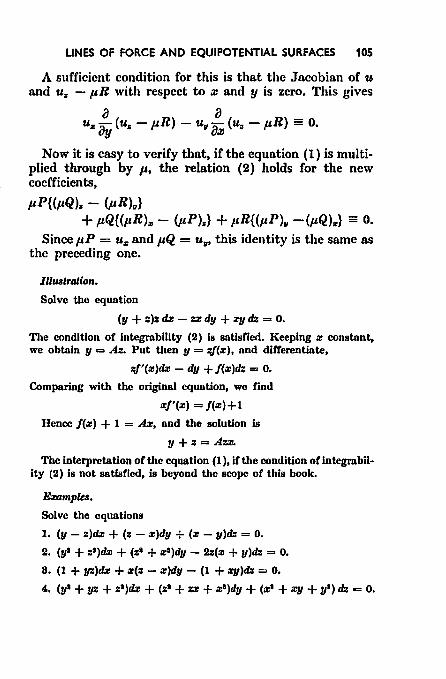
An appendix has been added on Laplace transforms and one on the equation Ptk + Qdy + Rdz = 0. The interest of these topics may be manipulative rather than theoretical, but the student who wishes to be informed on them will be spared the necessity of turning to a different book.
May 1961. .T. C. B.
CONTENTS
CIIAl'TER J
EXISTENCE OF SOLUTIONS
1. Some problems for investigation 2. Simple ideas about solutions 8. Existence of a solution 4. Extensions of the existence theorem
CRAFl'ER lJ
THE LINEAR EQUATIOS
5. Existence theorem 6. The linear equation 7. Independent solutions 8. Solution of non-homogeneous equations 0. Second-order linear equations
10. Adjoint equations
CHAPTER JJl
OSCILLATION THEOREl\IS
11. Convexity of solutions 12. Zeros of solutions 18. Eigenvalues 14. Eigenfunctions and expansions
CHAPTER JV
SOLUTION IN SERIES
15. Differential equations in complex variables 16. Ordinary and singular points
vii
PAGE
1 2 4 8
12 18 13 17 18 20
25 ?:'/ 20 81
83 84
CONTENTS
17. Solutions near a regular singularity 86 18. Convergence of the power series 88 19. The second solution when exponents are equal or differ by
an integer 80 20. The method of Frobenius 40 21. The point at infinity 42 22. Bessel's equation 42
CIIAPl'ER V
SINGULARITIES OF EQUATIONS
28. Solutions near a singularity 2-1. Regular and Irregular singularities 25. Equations with assigned singularities 26. The hypergcometric equation 27. The hypergeometric function 28. Expression of F(a, b; c; z) as an integral 20. Fonnulae connecting hypergeomctric functions 80. Confluence of singularities
CIIAPl'ER VI
CONTOUR INTEGRAL SOLUTIONS
81. Solutions expressed as integrals 82. Laplace's linear equation 88. Choice of contours 84. Further examples ot contours 85. Integrals containing a power or C - z
CHAPTER VII
LEGENDRE FUNCTIONS
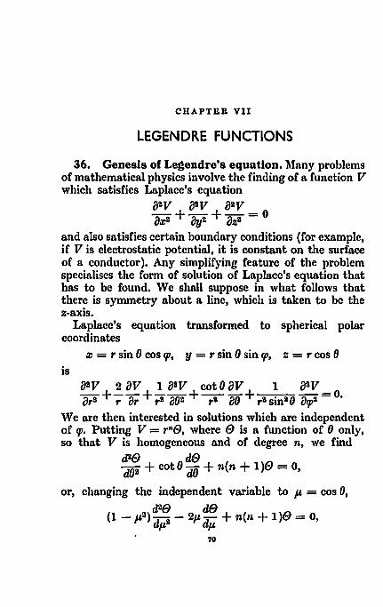
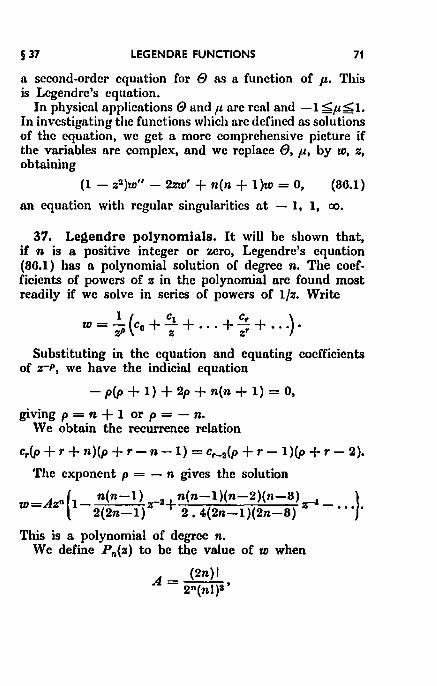
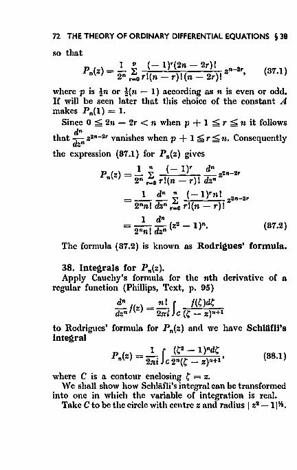
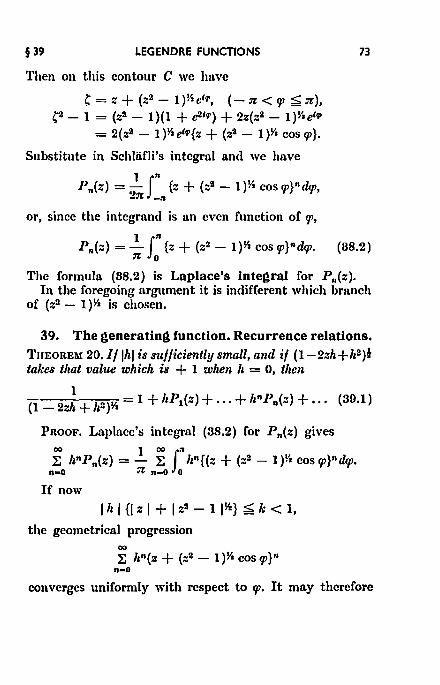
86. Genesis of Legendre's equation 87. Legendre polynomials 88. Integrals for P,.(::) 89. The genemting function. Recurrence relations 40. The function P,.(z) for geneml v
47 49 61 52 liB 64 65 57
59 59 62 68 05
70 71 72 78 74
CONTENTS ix
CILU'TER VIII
BESSEL FUNCTIONS
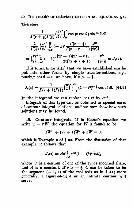
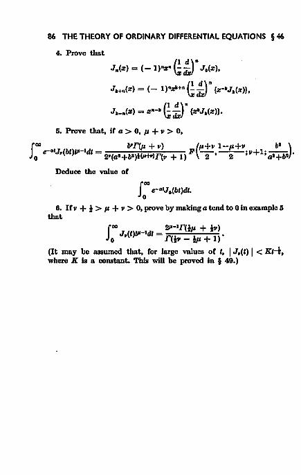
41. Genesis of Bessel's equntion 77 42. The solution J.(::) in series 78 43. The genemting function for J,.(::). Heeurrence relations 79 44. Intcgmls for J.(::) 81 45. Contour integmls 82 40. Application of oscillntion theorems 83
CllAI'TER IX
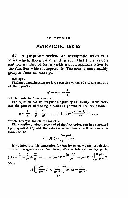
ASYMPTOTIC SERIES
47. Asymptotic series 87 48. Definition and properties of nsymptotic series 88 49. Asymptotic expansion of Bessel function 90 50. Asymptotic solutions or differential equations 94 51. Calculation of zeros of J 0 {x) 95
APPENDIX 1. The Laplace tmnsCorm 97
APPENDIX u. Lines of force and equipotential surfaces lOS
SoLUTIONS OF EXAMPLES 109
BIBLIOGRAPHY 113
INDEX 114
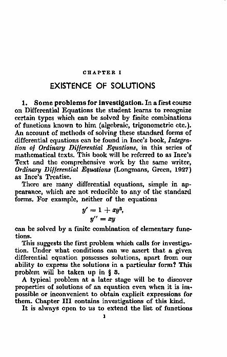
CHAPTER I
EXISTENCE OF SOLUTIONS
1. Some problems for investigation. In a first course on Differential Equations the student )earns to recognize certain types which can be solved by finite combinations of functions known to him (algebraic, trigonometric etc.). An account of methods of solving these standard forms of differential equations can be found in Incc's book, Integration of Ordinary Di!Jerential Equations, in this series of mathematical texts. This book will be referred to as Incc's Text and the comprehensive work by the same writer, Ordinary Dijjerential Equations (Longmans, Green, 1927) as !nee's Treatise.
There arc many differential equations, simple in appearance, which arc not reducible to any of the standard forms. For example, neither of the equations
y' = 1 + ccys, y" = tcy
can be solved by a finite combination of elementary functions.
This suggests the first problem which calls for investigation. Under what conditions can we assert that a given differential equation possesses solutions, apart from our ability to express the solutions in a particular form? This problem will be taken up in § 8.
A typical problem at a later stage will be to discover properties of solutions of an equation even when it is impossible or inconvenient to obtain explicit expressions for them. Chapter III contains investigations of this kind.
It is always open to us to extend the list of functions 1
l THE THEORY OF ORDINARY DIFFERENTIAL EQUATIONS § 2
which are regarded as available for solving differential equations. If an equation, not of one of the standard forms, has many applications, say to problems of physics, it may be worth while to give names to its solutions and thus define new functions; we can study their properties and make tables of their values. The equation y" = IXIJ just mentioned (Airy's equation), which presents itself in problems of diffraction, gives rise to functions called Ai(a!) and Bi(a!). These functions lie outside the scope of this book, but an account will be given in Chapters VII and VIII of the more important functions, Legendre's and Bessel's, arising from differential equations which occur repeatedly in applied mathematics.
2. Simple ideas about solutions. Consider the firstorder equation
y' = /(a!, y). (2.1) To solve this equation we have to find the functions y = y(x) which satisfy it for all values of a! in an appropriate interval, say a - h ~ x ~ a + h. The geometrical interpretation is that the curve y = y(x) has at every point a tangent whose gradient is determined by (2.1).
Geometrical intuition leads us to expect that a solution will exist through a given point x = a, y = b, and that we can construct the curve representing it by a process such as the following. Draw a short segment of a straight line from (a, b) with gradient /(a, b) to the point (xu y1 ).
From (x1, y1 ) draw a short segment with gradient j(x1, y1 )
to (x2, y2); and so on, to (x,., y,.) say. We thus follow the gradient prescribed by the differential equation. It is at least plausible that, as the lengths of the segments in the construction are decreased, the polygons will approximate to a curve for which y' = j(x, y).
These indications, which do not profess to prove anything, can be developed into a formal argument. 'V c shall in fact adopt a rather different approach to the existence theorem.
§2 EXISTENCE OF SOLUTIONS 3
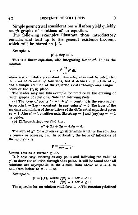
Simple geometrical considerations will often yield quickly rough graphs of solutions of an equation.
The following examples illustrate these introductory remarks and lead up to the general existence-theorem, which will be stated in § 3.
E:eample 1. y' + 2zy =I.
This is a linear equation, with integrating factor & 1• It has the
solution
y = e--r J: e11 dt,
where a is an arbitrary constant. This integral cannot be integrated in tcnns or elementary functions, but it def"mes a function or z, and a unique solution or the equation exists through any assigned point of the (z, y) plane.
The reader may use this example for practice in the drawing of rough graphs of solutions. Note the following facts.
(a) The locus of points Cor which y' = constant is the rectangular hyperbola 1 - 2zy = constant. In particular y' = 0 (U1e locus of the maxima and minima of the solutions of the differential equation) gives :7:11 = l.Alsoy' =I oneiU1eraxis.Sketch:7:1J =!and (say):7:11 = ± 1 us guides.
(b) Differentiating, we find that
y'' + 2z + 2y - .uay = 0. The sign of y" for a given (z, y) determines whether the solution
is convex or concave, and, in particular, the locus of inflexions of the solutions is
:t y= ---· 2zl- I
Sketch this as a further guide. It is now easy, starting at any point and following the value of
y', to draw the solution through that point. It will be found that all solutions are nsymptotie to the z-axis, from above us :e -+ + co and from below as :e -+ - co.
E:wmple 2. y' = J(z), where J(z) = 0 Cor :e < 0
nnd f(z) = 1 for :t ~ o. Tbe equation has no solution valid for :t = o. The function y defined
4 THE THEORY OF ORDINARY DIFFERENTIAL EQUATIONS § 3
by y = C form < 0 andy = m + C form ;::;:; 0 is a continuous function satisfYing the equation for all oU1er values of z, but it has no derivative at :z = 0. Plainly the failure is due to the discontinuity of J(z).
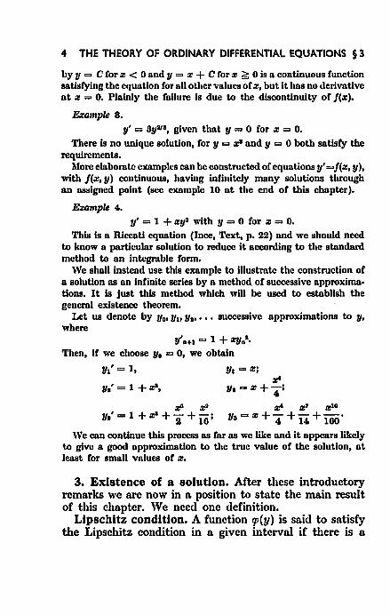
&le 8.
y' = 3y111, given that 1/ = 0 for 01: = o. There is no unique solution, for y = z:l and y = 0 both satisfy the
requirements. l\Iore elaborate examples can be constructed of equations y' = f(z, y ),
wiUl J(:z, y) continuous, having infinitely many solutions through an osslgned point (see example 10 at the end or this chapter).
Ezample 4.
y' = 1 + a:y1 with y = 0 for m = 0. This is a Riccati equation (lnce, Text, p. 22) and we should need
to know a particular solution to reduce It according to the standard method to an integrable form.
We shaD instead use this example to Illustrate the construction of a solution as an Infinite series by a method or successive approximations. It is just this method which lViU be used to establish the general existence theorem.
Let us denote by y0, y1, y1, ••• successive approximations to y, where
1/'a+l = 1 + 4:1Ja1•
Then, if we cboose Yo = 0, we obtain
lh' = 1,
1Ja' = 1 + z:l, z'
Ya = z +4• a:' m' mto
Ya = m + 4 + 14 + 160'
We can continue this process as Car as we like and it appears likely to give a good approximation to the true value of the solution, at least Cor small values of m.
3. Existence of a solution. After these introductory remarks we are now in a position to state the main result of this chapter. We need one definition.
Lipschitz condition. A function q;(y) is said to satisfy the Lipschitz condition in a given interval if there is a
§3 EXISTENCE OF SOLUTIONS 5
constant A such that
ltp(Yl) - tp(Ya)l ~ AiYt - Yzl
for every pair of values Y~t y1 in the interval. We observe that the condition is certainly satisfied if
jtp'(y)l ~A. Its usefulness is that it leads to much the same consequences as the hypothesis of a bounded derivative, but the restrictive assumption that the derivative exists at every point is avoided.
THEOREM 1. Let f(z, y) be continuous in a domain D of the (z, y) plane and let M be a constant such thai, lf(m, y)l < M in D. Let f(m, y) sati8fy in D tile Lipschitz condition in y,
where the constant A is independent of m, y1, y2•
Let the rectangle R, defined by
lm - al ~ h, ly - bl ~ k, lie in D, where lJfh < k. Then, for jm - aj ~ h, the differential equation
y' = f(m, y)
has a unique solution y = y(m) for which b = y(a).
PROOF. Define the sequence of functions
Yo(m) = b,
Y1(m) = b + J: f{t, y0(t)}clt,
Yll(m) = b + J: f(t, y1(t)}dt,
yfl(m) = b + J: f{t, Yt~-1(t)}dt. We shnU prove that, as n-+ oo, lim Yn(.v) gives the
required solution. There nrc several steps in the proof. (i) We prove that, for a - h ~ m ~ a + h, the curve
y = Yn(m) liesintllerectangle R, that is to say b-k<y<b+k.
6 THE THEORY OF ORDINARY DIFFERENTIAL EQUATIONS § 3
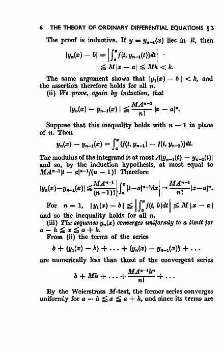
The proof is inductive. If y = y,_1(t.ll) lies in R, then
ly,(x) - bl = IJ: f{t, Yn-1(t)}dtl •
~ M jt.ll- al ~ Mh < k.
The same argument shows that ly1(t.ll)- b I< k, and the assertion therefore holds for all n.
(ii) We prove, again by induction, that
ltJ.An-1 IYn(X) - Yn-1(m) I ~ ----n1 1111 - al"·
Suppose that this inequality holds with n - 1 in place of n. Then
y,(m) - Yn-1(x) = J: U(t, Yn-1) - f(t, Yn-ll)}dt.
The modulus of the integrand is at most .AIYn-1(t) - Yn-:a(t)l and so, by the induction hypothesis, at most equal to M.A"-11t- alll-1/(n- 1)1 Therefore
M.An-l I 111 I ltJ.An-1 ly,(m)-Yn-l(m}l ~ (n-l)l a 1t-aln-ltL7J = ----;;r-lm-al"·
For n=l, ly1(m)-bl ~\J:f(t,b)dtl ~Mlt.ll-al and so the inequality holds for all n.
(iii) The sequence Yn(a:) converges uniformly to a limit for a-h~mS:a+h.
From (ii) the terms of the series
b + {yl(a:) - b} + • • • + {yn(t.ll) - Yn-l(x)} + • • • are numerically less than those of the convergent series
ltJ.An-1hn b + Mh + ... + nl + ...
By the ·weierstrass M-test, the former series converges uniformly for a - h ;;a;; m ~ a + h, and since its terms are
§3 EXISTENCE OF SOLUTIONS 7
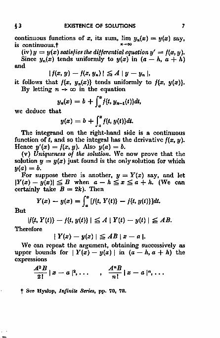
continuous functions of x, its sum, lim y,.(x} = y(x} say, is continuous. t n .... co
(iv) y = y(x} satisfies the diflerential equation y' = f(x, y). Since y,.(x} tends uniformly to y(x} in (a- h, a+ h)
and I f(x, y} - /(x, y,.} I ~ A I y - y,. 1.
it follows that f{x, y,.(x}} tends uniformly to f{x, y(x}}. By letting n -+- oo in the equation
y,.(x} = b + J: f{t, Yn-l(t)}dt,
we deduce that
y(x} = b + J: f{t, y(t)}dt.
The integrand on the right-hand side is a continuous function oft, and so the integral has the derivative f(x, y}. Hence y'(x} = f(x, y}. Also y(a} = b.
(v} Uniqueness of the solution. We now prove that the solution y = y(x} just found is the only solution for which y(a} =b.
For suppose there is another, y = Y(x} say, and let IY(x}- y(x}l ~ B when a- h ~ x ~a+ h. (We can certainly take B = 2k ). Then
Y(x} - y(x} = J: [J{t, Y(t)} -f{t, y(t)}]dt.
But
1/{t, Y(t}} - f{t, y(t)} I ~ A I Y(t) - y(t} I ~ AB. Therefore
I Y(x} - y(x} I ~ AB I x - a I· ·we can repeat the argument, obtaining successively as
upper bounds for I Y(x} - y(x) I in (a - h, a + h) the expressions
ABB A"B 21' Ill - a 111
, • • • , nr' Ill - a 1", ...
t See Hyslop, Infinite Series, pp. 70, 73.
8 THE THEORY OF ORDINARY DIFFERENTIAL EQUATIONS § 4
But this sequence tends to 0 and so Y(m) = y(x) in (a- h, a+ h), and the proof of the theorem is complete.
A slightly different version of the above theorem is sometimes useful; we state it as a Corollary.
CoROLLARY. Let f(x, y) be continuous for a. ~ m ~ p and all y. Let it satisfy the Lipschitz condition of the theorem. Then, given a, b, with a. ~ a ~ p, the equation y' = f(m, y) ha8 a unique solution y = y(m) for a. ~ m ~ p for which b = y(a).
To establish the corollary we adapt the argument of theorem 1 by omitting the step (i) and defining the 1lf in (ii) and (iii) to be the upper bound of lf(x, b) I for a. ;;i m ;;i p.
4. Extensions of the existence theorem. The basic existence theorem of § 8 may be elaborated in a number of ways, some of which will be outlined.
THEOREl!.l 2. With the hypotheses of Theorem 1, suppose that y = Y(m) is the solution for which Y(a} = b +d. Then, for lx - a I ::=;; h,
!Y(x) - y(m) 1 ;;i deAA. This means that a small change in the initial conditions
causes only a small change in the solution throughout an interval.
PnooF. Construct a sequence Yn(m) by the rules
Y0(x) = b + 15, Y1(m) = b + 15 +I: f{t, Y 0(t)}dt, t • • • • • • • • • • • • • •
Yn(m) = b + 6 +I: f{t, Y~a_1(t)}dt. As before, Yn(x) converges to the solution Y(x).
I Y 1(m)- y1(x) I ;;i 6 + IJ:If(t, b +d)- f(t, b) ldtl /
~6+A61x-al. ~
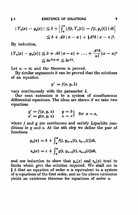
§4 EXISTENCE OF SOLUTIONS
I Y2(x) - y11(x) I ~ c5 + I J: 1/{t, Y1(t)} - f{t, Y1(t)} I dt I ~ c5 + Ac5 I x - a I + !A2c5 I x - a p.1.
By induction,
9
A"c5 IY,.(x)- y,.(x)l ~ c5 + Ac51x-al + ... + -
1 lx- al" n
~ c5eAI4>-ol ~ c5eAr•.
Let n -+ co and the theorem is proved. By similar arguments it can be proved that the solutions
of an equation
y' = f(x, y, ).)
vary continuously with the parameter ).. Our next extension is to a system of simultaneous
differential equations. The ideas are shown if we take two equations
y' = f(x, y, z) z' = g(a:, y, z)
Y = b } for a: = a Z=C '
where I and g are continuous and satisfy Lipschitz conditions in y and z. At the nth step we define the pair of functions
y,.(a:) = b + J: f{t, Yn-l(t), Zn-l(t)}dt,
z,.(x) = c + J: g{t, Yn-l(t), Zn-l(t)}dt,
and use induction to show that y,.(x) and z,.(x) tend to limits which give the solution required. We shall see in § 5 that an equation of order n is equivalent to a system of n equations of the first order, and so the above extension yields an existence theorem for equations of order n.
10 THE THEORY OF ORDINARY DIFFERENTIAL EQUATIONS § 4
Examples. • - 4k •
I. Show that, 1f m_ = - 2k + I , the equation
y' + y• = az"' • 4k
can be reduced to one of similar form in which m = - 2k _ 1
by
putting m"'+1 =X, (m + l)y = aJY; and show that the new equation can be reduced to one of the old form with k - I in place of k by
I I f1 putting X = T' Y = X - XS •
Solve the equation
y' + Y' = r"•. 2. Show that, it Yo is any particular integral of
(I) y' = p(m)y• + q(m)y + T(z),
then the function I/(y- y0) satisfies a linear differential equation ot the first order.
Show that the cross-mtio of any four given particular integrals of (1) is independent of m. Verily that cot m is a solution of the equation
2y' + y1 sec1 :11 - y sec m cosec m + 2 cosec1 m = O,
and f'md the general solution.
8. If f(m) -+ l oa m -+ co, prove that, if a > o, every solution of the equation
y' + ay =f(m) tends to the limit lfa as m-+ co. If, however, a < o, only one solution tends to lfa.
4. Sketch the solutions of each of the equations
1 1 (a) y' + y = m' (b) y'- y = -;;·
5. Sketch the solutions of each of the equations
(a) y' = 1111 + y1 - 1, 1
(b) y' = 1 - m1 - y1 '
What relation is there between the two sets of curves?
§4 EXISTENCE OF SOLUTIONS 11
6. Verify that Ute process of successive approximation or § 8 applied to the equation y' = ky yields the known solution. Curry out the same verification for the pair of simultaneous equations
y' = z, ::' = - y (y = 0, :: = 1, when :z: = 0).
7. Find the solution, for :z: ~ 0, of the equation
y' = max (:z:, y), y(O) = 0.
8. Find the solutions, as far as Ute terms in :z:l, or the equations
(i) y' = zs + siny, (ii) y' = :z:z,
='=:r+y,
y(O) = 0; y(O) = 0, ::(0) = 1.
9. Discuss the behaviour ncar the origin of solutions of the equation
(am- bl ::/= 0),
distinguishing the cases (b - l)s + 4am > 0, = 0 or < 0.
10. Define J(:r, y) so that the equation y' = J(:t, y) shall have solutions
y = A:z:1 for - 1 ;:;;; A ;:;;; 1 it I y I ;:;;; :~:1, y = z• + B tor B > 0 if y > z', y = - z1 - B it y < - :z:s.
Prove that j(:r, y) is continuous at (0, 0).
11. R1(:z:), R1(11l) nrc continuous, and R1 > R1, in 0 ;:;;; :t ~a, and F(:z:, y) is continuous In (:r, y) for 0 ~ :r ~a and all y. Given that y10 y1 are solutions In 0 ~ :z: $ a of
y' = F(:r, y) + R1(:z:)
respectively wiUt y1(0) ~ y1(0), prove tlmt y 1 > y1 in 0 < :t ~a. Show that the equation
y' = 1 + y1 + :r1 (:r ~ 0), y(O) = 0
has a solution with a vertical asymptote z = z0 , where z 0 ~ ~.
CHAPTER II
THE LINEAR EQUATION
5. Existence theorem. Our next task is to obtain an existence theorem for solutions of the nth order equation
yin) = j(a:, y, y', , , ,, yln-1) ),
where ylnl denotes the nth derivative of y. Suppose that, for a value E of a:, the values of
y, y', ••. , yln-u are given to be ?'J• ?'Ju ••• , t'Jn-1 respectively. What conditions on f arc sufficient to ensure the existence of a unique solution of the equation in an interval containing e? As we have already remarked on page 9 this problem can be reduced to that of n first-order equations with a: as independent variable and n dependent variables which we shall call y0, Yv ••. , Yn-1•
The system of equations
Yo= Y1• y). = Y2•
Y~-~ = Yn-1• Y~-1 = f(a:, Yo• Yt• • • ·• Yn-1),
with the initial conditions that Yo = rJ• y1 = ?]1, ••• ,
Yn-1 = t'Jn-1 for a: = E is equivalent to the given nth order equation.
The work on page 9 then yields the following existence theorem.
TnEOREI\1 8. If f(a:, y, y', ... , yln-U) is a continuous function of its n + I variables in a given n + 1 dimensional domain D and satisfies a Lipschitz condition in each of
18
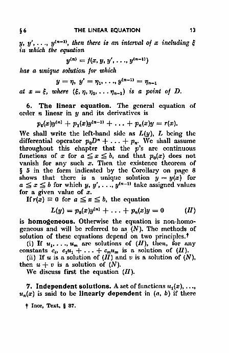
§6 THE LINEAR EQUATION 13
y, y', ••. , y<n-u, then there is an interoal of x including ~ in which the equati()n
y<nl = f(x, y, y', • , ., y<n-11)
has a unique solution for which
Y = '11• y' = '111• • • •t y<n-1l = 1/n-1
at X = ~. where (~, 7J• 7J1, •• ·'lln-t) is a point of D.
6. The linear equation. The general equation of order n linear in y and its derivatives is
Po(x)ylnl + Pt(x)yln-11 + . , . + Pn(x}y = r(x).
We shall write the left-hand side as L(y), L being the differential operator poiJn + ... + Pn· We shall assume throughout this chapter that the p's arc continuous functions of x for a ::;;: x ~ b, and that p0(x) does not vanish for any such x. Then the existence theorem of § 5 in the form indicated by the Corollary on page 8 shows that there is a unique solution y = y(x) for a ::;;: x::;;: b for which y, y',, . . , y<n-11 take assigned values for a given value of x.
If r(x} = 0 for a ::;;: x ::;;: b, the equation
L(y) = p0(x)ylnl + ... + Pn(x)y = 0 (11}
is homogeneous. Otherwise the equation is non-homogeneous and will be referred to ~ (N}. The methods of solution of these equations depend on two principles. t
(i) H u1, ••• , Um are solutions of (H), then, for any constants c1, c1u1 + ... + c,1Um is a solution of (H).
(ii) If u is a solution of (II) and v is a solution of (N), then u + v is a solution of (N).
We discuss first the equation (H).
7. Independent solutions. A set of functions tt1(x), ... , tln(x) is said to be linearly dependent in (a, b) if there
t Ince, Text, § 87.
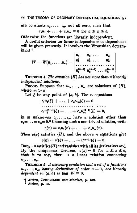
14 THE THEORY OF ORDINARY DIFFERENTIAL EQUATIONS § 7
are constants c1, ••• , en, not all zero, such that
c1u1 + ... + Cntln = 0 for a ~ a: ~ b. Otherwise the functions are linearly independent.
A useful criterion for linear independence or dependence will be given presently. It involves the Wronskian determinant t
ua •• • u8 •••
u.!n-1) .,(n-1) .,(n-1) -1 "'I • • • "'n
THEOREM 4. The equation (H) hM not more than n linearly independent solutions.
PRooF. Suppose that ftt, .•• , um are solutions of (H), where m > n.
Let E be any point of (a, b). The n equations
c1u&~) + ... + CmUm(~) = 0
clufn-1)(~) + ... + Cmu!:-ll(E) = 0,
in m unknowns c1, ••• , em have a solution other than c1 = ... = Cm=O. *Choosing such a non-trivial solution, write
v(a:) = c1u1(a:) + ... + Cmum(a:).
Then v(a:) satisfies (H), and the above n equations give v(E) = v'(E} = ... = vln-ll(~) = 0.
Buty= 0 satisfies(H)and vanishes with all its derivatives atE. By the uniqueness theorem, v(a:) = 0 for a ~a:~ b, that is to say, there is a linear relation connecting "to • • • Um•
THEOREM 5. A necessary condition that a set of n functions u1, ••• , Un, having derivatives of order n - 1, arc linearly dependent in (a, b) is that W = 0.
t Aitken, Determinants and Matrices, p. 132. • Aitken, p. 68.
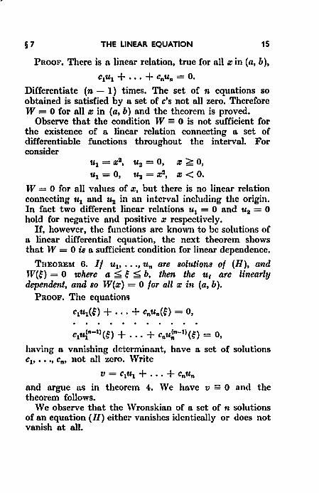
§7 THE UNEAR EQUATION 15
PRooF. There is a linear relation, tn1e for all a: in (a, b),
CiUl + . , . + CnUn = 0.
Differentiate (n - 1) times. The set of n equations so obtained is satisfied by a set of c's not all zero. Therefore W = 0 for all a: in (a, b) and the theorem is proved.
Observe that the condition W = 0 is not sufficient for the existence of a linear relation connecting a set of differentiable functions throughout the interval. For consider
u1 = afl, u 2 = 0, a: ~ 0,
u1 = o, u2 = xll, a: < o. W = 0 for all Yalues of a:, but there is no linear relation connecting u 1 and u8 in an interval including the origin. In fact two different linear relations u1 = 0 and u2 = 0 hold for negative and positive :c respectively.
If, however, the functions are known to be solutions of a linear differential equation, the next theorem shows that W = 0 i8 a sufficient condition for linear dependence.
THEOREl'rf 6. If u1, ••• , Un arc solutions of (H), and W(E) = o where a :::;; e ~ b, then the u1 arc linearly dependent, and so W(a:) = 0 for all :c in (a, b).
PRoOF. The equations
CtUt(~) + • • • + CnUn(E) = 0,
ctufn-1)(~) + ... + c,.u~n-ll(E) = 0,
having a vanishing determinant, have a set of solutions c1, ••• , en, not all zero. Write
V = C1U1 + ... + CnUn
and argue as in theorem 4. We have v = 0 and the theorem follows.
We observe that the Wronskian of a set of n solutions of an equation (II) either vanishes identically or docs not vanish at all.
16 THE THEORY OF ORDINARY DIFFERENTIAL EQUATIONS § 7
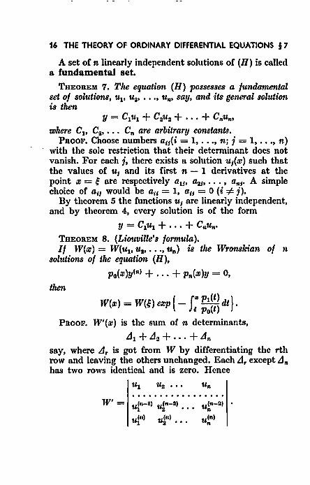
A set of n linearly independent solutions of (H) is caJled a fundamental set.
THEOREM 7. The equation (H) possesses a fundamental set of solutions, Ut• u11, ••• , un, say, and its general solution uthen
y = C1u1 + C2u11 + ... + CnUno
where C1, C2, ••• Cn are arbitrary constants. PROOF. Choose numbers a11(i = 1, ... , n; i = 1, •.• , n)
with the sole restriction that their determinant does not vanish. For each j, there exists a solution u1(w) such that the values of u1 and its first n - 1 derivatives at the point a: = E are respectively a11, ~ •••• , ans• A simple choice of ail would be a11 = 1, ail = 0 (i =I= j).
By theorem 5 the functions u1 are linearly independent, and by theorem 4, every solution is of the form
y = C1u1 + , .. + CnUn•
THEoREM 8. (Liouville's formula). If W(a:) = W(Ut, U2, ••• , Un) is the Wronskian of n
solutions of the equation (H),
Po(.v)ylnl + • • • + Pn(w)y = O,
then
W(a:) = W(E) e.vp { - J" Pt(t) dt}. f p0(t)
PnooF. W'(.v) is the sum of n determinants,
Ll1 + Ll11 + • • • + Ltn say, where Ltr is got from W by differentiating the rth row and leaving the others unchanged. Each Ltr except Ltn has two rows identical and is zero. Hence
W' = uCn-111 ,Jn-111 1 ..... l: •••
ufnl t4n),,,
§8 THE LINEAR EQUATION 17
In the last row, substitute for each ulnl from the equation
Poulnl = -p.uln-11 - • • • - PnU
and again omit vanishing determinants. This gives p0(x)W'(x) = - p1(x)W(x).
Integrating this equation, we have the theorem.
8. Solution of non-homogeneous equation. If a fundamental set of solutions of the homogeneous equation has been found, the equation
L~)=~x) (N) can be solved by Lagrange's method of variation of parameters.
Let u1, ••• , ttn be n independent solutions of (H). Write
y = V1u1 + ... + Vnttno
where the V's, instead of being constants, will be functions of x.
y' = V1tt1 + ... + Vntt~ + [Vi'u1 + ... + V~un]• The V's will be chosen to make the sum of the terms within square brackets vanish for all x.
Continuing, we have
y" = V1ul.' + ... + Vntt~' + [V!ul. + ... + V~tt~]. Again make the sum of the terms in square brackets zero. Repeat this process up to yln-ll, Finally,
ylnl = y 1ufn1 + ... + Vntt~nl + [Viufn-11 + ... + V~u~n-tl]. l\lake the sum of the terms in these square brackets equal to r(x)/p0(x).
1\lultiplying the expressions for ylnl, ••• , y', y by p0, ••• , Pn-l• Pn respectively and adding, we see that y satisfies (N).
The values assigned to the square brackets provide n equations for V{, •• . , V~. The determinant of the coefficients is the Wronskian of the u's and is consequently
18 THE THEORY OF ORDINARY DIFFERENTIAL EQUATIONS § 9
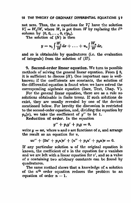
not zero. Thus, the n equations for v; have the solution V/ = W,fW, where W, is got from W by replacing the ith column by (0, 0, ••• , 0, r/p0).
The solution of (N) is then
Y = U. J i dz + • • • + Un J ~ dz,
and so is obtainable by quadratures (i.e. the evaluation of integrals) from the solution of (H).
9. Second-order linear equation. We turn to possible methods of solving the general linear equation. From § 8, it is sufficient to discuss (H). One important case is wellknown; if the coefficients are constants, the solution of the differential equation is found when we have solved the corresponding algebraic equation (Ince, Text, Chap. V).
For the general linear equation, there are as a rule no solutions obtainable in finite terms. If such solutions do exist, they are usually revealed by one of the devices mentioned below. For brevity the discussion is restricted to the second-order equation, and, dividing the equation by p0(m), we take the coefficient of y" to be 1.
Reduction of order. In the equation
y" + P1Y' + P'J!J = 0,
write y = uv, where u and v are functions of a~, and arrange the result as an equation for v,
uv" + (2u' + p1u)v' + (u" + p1u' + p11u)v = 0.
If any particular solution u of the original equation is known, the coefficient of v in the equation for v vanishes and we are left with a linear equation for v', and so a value of v containing two arbitrary constants can be found by quadratures.
The same method shows that a knowledge of a solution of the nth order equation reduces the problem to an equation of order n - 1.
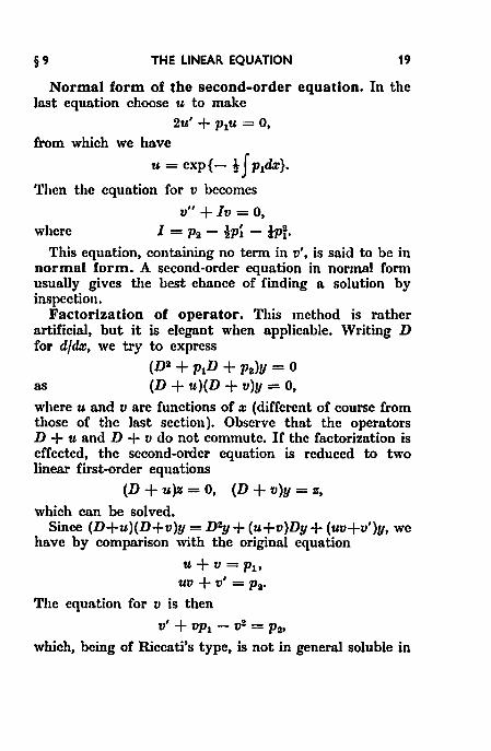
§9 THE LINEAR EQUATION 19
Normal form of the second-order equation. In the last equation choose u to make
2u' + p1u = 0,
from which we have
u = exp{-! J Pld.x}.
Then the equation for v becomes
v" + Iv = 0,
where 1 = Pa - !P~ - iJJJ. This equation, containing no term in v', is said to be in
normal form. A second-order equation in normal form usually gives the best chance of finding a solution by inspection.
Factorization of operator. This method is rather artificial, but it is elegant when applicable. Writing D for dfdx, we try to express
(D3 + P1D + Pa)Y = 0 as (D+u)(D+v)y=O,
where u and v are functions of a: (different of course from those of the last section). Observe that the operators D + u and D + v do not commute. If the factorization is effected, the second-order equation is reduced to two linear first-order equations
(D + u)z = 0, (D + v)y = z,
which can be solved. Since (D+u)(D+v)y =Dig+ (u+v)Dy+ (uv+v')y, we
have by comparison with the original equation
u + v = Pl• uv + v' = p 3•
The equation for v is then
v' + vpl - v~ = Pt~•
which, being of Riccati's type, is not in general soluble in
lO THE THEORY OF ORDINARY DIFFERENTIAL EQUATIONS § 10
finite terms, even for an equation in normal form with Pt = o.
10. Adjoint equations. It is natural to ask whether a search for an integrating factor will help towards solving the second-order equation. Taking
L(y) = PoY" + PtY' + P'JJ/t can we find a function z of a: such that
d zL(y) = da: L 1(y),
where L1(y) is a differential operator of the first order? Integrating by parts, we have
f zL(y)d.v = pozy'- (poZ)'y + f (PoZ)"yda:
+ PtZV - f (ptz)'yda:
+ f p<f4yd.v.
The integrals on the right-hand side vanish, making zL(y) an exact differential if z satisfies
M(z) = (PoZ>'' - (ptz)' + Pr = o. So the finding of an integrating factor involves the
solution of another second-order equation and we are generally no better off.
The operator M is called the adjoint of L. From the above argument, we have Laflrange's identity
zL(y)- yM(z) = ! {p0(y'z- yz') + (Pt - Po)yz}.
It is easy to verify that the relation of being adjoint is reciprocal; Lis the adjoint of }Jf. If L, Mare the same, the equation is self-adjoint. The necessary and sufficient condition for this is that p1 = p~. and the equation in
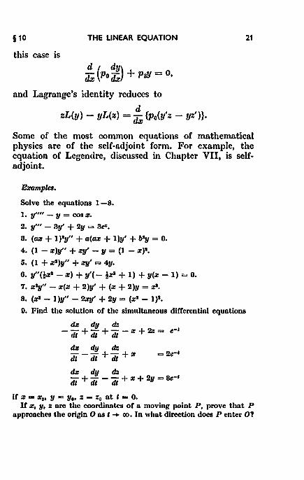
§10 THE LINEAR EQUATION 21
this case is
d ( dy) d:e Po d:e + P'l!l = o,
and Lagrange's identity reduces to
d zL(y) - yL(z} = d:e {p0(y'z - yz')}.
Some of the most common equations of mathematical physics are of the self-adjoint form. For example, the equation of Legendre, discussed in Chapter VII, is selfadjoint.
f'md a first-order differential equation, not involving 11, satisried by u.
Apply this to the equation
cPy dy 2 dJll- tanz dz -1 + sinm 11 = O;
using the substitution u cos m = .:, or otherwise, f'md a solution for u and hence solve completely the given equation.
14. Show that, if /(m) Is continuous for :11 fi:!i 1, then the solution ot the equation
my"' - y" + IZ1I - y = /(m)
that Is valid for m fi:!i 1 Md is such that 11" = y' = 11 = 0 when m = 1 may be written In the form
§ 10 THE LINEAR EQUATION
y = I: f(t)g(:r, t)dt,
ami determine the function g(:r, t).
23
15. Show that a necessary and sufficient condition for the ex-pression
rPy dy P(z) dzl + Q(z) d;e + R(:r)y
to be expressible in the form
d { dy } d;e L(z) d;e + M(x)y
is that P"(x) - Q'(z) + R(x) = o.
Solve completely the differential equation
d~y dy z(1 + x) dJ:I - {n + (n - 2).r} dJ: - ny = zn+l.
16. Prove that the differential equation
:ry" + 2ny' + k;ry = 0,
where n is a positive integer and k a real constant, is satisfied by
y = (2. ~)nu X d;e '
where u is a solution of the equation
u" + ku = o. Find the solution of the differential equation
:ry" + 4y' + :ry = 0
for which y = 0 and y' = 1 when x = :r; prove that, when z = 2:r, y = 1/(S:r).
17. Let u1(z), ••• , u.(z) be continuous in (a, b). Write
(1 -;;[, i,j ;;in).
Let G be the determinant of order n (the Gramian) whose clements arc a11• Prove that G = 0 is a necessary and sufficient condition for the linear dependence of u1(z), ••• , u,.(z) in (a, b).
24 THE THEORY OF ORDINARY DIFFERENTIAL EQUATIONS § 10
18. If c1u,_(:~:) + c1u1(:~:) is the general solution of the equation y" + p1y' + p.y = 0, obtain the general solution of the adjoint equation.
19. Solve the equation
(z + 1)zly'' + :ry'- (z + 1)'1/ = 0,
given thnt there ore two solutions whose product is n constant. (This example illustrates Ute principle thnt a given fact about
solutions, holding throughout on interval or values or z, can often be used to reduce by one the order or the differential equation).
20. If Ute equation y" + p.y' + p.y = 0 has two solutions whose product Is o. constant, find the relation between p 1 and p 1•
CHAPTER III
OSCILLATION THEOREMS
11. Convexity of solutions. The theorems of this chapter show that, although we cannot in general obtain explicit solutions of second-order equations, a good deal can be said about their behaviour. Theorems like 12 and 18, which deal with zeros of solutions, their distance apart etc., are typical and give the title to the chapter.
Consider the homogeneous equation in normal form
y" + g(x)y = 0,
where g(x) is continuous. The key-note of theorems 9 and 10 is that the sign of y" determines whether the curve y = y(x) is convex or concave.
THEOREM 9. If g(x) < 0 in tile interval (a, b), then any solution u(x) (not identically 0) of tile equation y" +g(x)y = 0 lias at most one zero in (a, b).
PnooF. Suppose that u(x0 ) = 0. Then u'(x0 ) ::f.= 0, for if u'(x0 ) = 0 then u(x) = 0 by the uniqueness theorem. If u'(x0 ) > 0, then there is an interval to the right of x0 in which u(x) is positive and so, for x > x0, the function u"(x) = - g(x)u(x) is positive; hence u'(x) is an increasing function. Therefore u(x) has no zero to the right of x0,
and similarly none to the left. A like argument holds if u'(x0 ) < 0. So u(x) has one zero or none in (a, b).
To obtain further results we take account of the magnitude of g(x). It will be helpful to compare two equations
y" + g(x)y = 0, (Y) z" + h(x)z = o. (Z)
116
26 THE THEORY OF ORDINARY DIFFERENTIAL EQUATIONS § 11
THEOREM 10. Let g(x) < h(x) for x :2: x0• Let y(x) be the solution of (Y) with the initial conditions y(x0 ) = y0 ,
y'(x0 ) = y~. these conditions being such that y(x) > 0 for some interval to the rigllt of x0• Let z(x) be the solution of (Z) satisfying the conditions z(x0 ) = y0, z'(x0 ) = y~. Then y(x) > z(x) for x > x0, so long as z(x) > o.
PROOF. (Y) and (Z) give
y"z - yz" = (h - g)yz.
Integrating from x0 to x, we have
y'z - yz' = r= (h - g)yzdx. Jzo
The right-hand side is positive so long as y and z are. . d (Y) y'z-yz' y . . . .
Smce d- - = 11 > 0, - 1s an mcreasmg function. X Z Z Z
But, for x = x0, yfz is 1 if Yo =I= 0 or tends to 1 if Yo = 0. The theorem follows.
COROLLARY 1. If y(~) = 0 for some~> x0, then z(q) = 0 for some 11 between x0 and ~.
ConoLLARY 2. If the values of y(x0 ), y'(x0 ) are such that y(x) < 0 for an interval to the riglll of x0, then the concl!Uion is that y(x) < z(x) so long as z(x) < o. Both cases are included in the statement I y(x) I > I z(x) I for x > x0, so long as z(x) does not van-ish.
The following calculation illustrates the use of,a comparison differential equation for estimates of magnitude of solutions.
If, in (Y), as x-+ oo, g(x) -+ -a11(a > 0), then, for arbitrarily small positive 11• any positive solution of (Y) satisfies the inequalitieB
elo-.,)z < y(x) < elo+.,l=
for all sufliciently large positive x. Take x0 large enough to make
(a -!17)11 < - g(x) < (a+ !11)11 for x ~ x0•
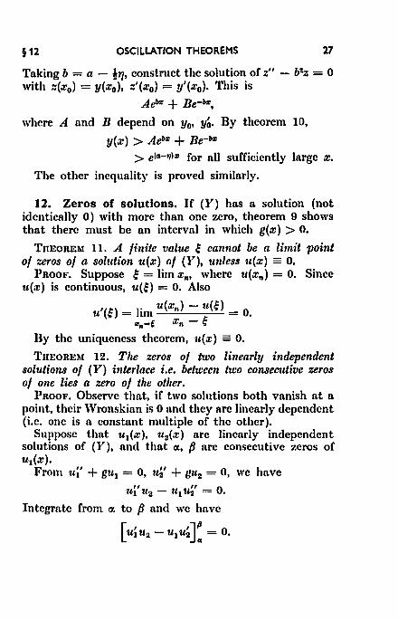
§12 OSCILLATION THEOREMS 27
Taking b = a - !17, construct the solution of z" - b'lz = 0 with z(.r0) = y(x0), z'(.r0) = y'(.r0). This is
A&=+ Be-b"',
where A and B depend on y0, y~. By theorem 10,
y(x) > A&:r: +Be-&"' > efa-ql:r: for all sufficiently large .r.
The other inequality is proved similarly.
12. Zeros of solutions. If (Y) has a solution (not identically 0) with more than one zero, theorem 9 shows that there must be an interval in which g(x) > 0.
THEOREM 11. A finite value ~ cannot be a limit point of zeros of a solution u(x) of (Y), unless u(.r) = 0.
PROOF. Suppose ~=lim Xn, where u(.rn) = 0. Since u(x) is continuous, u(~) = 0. Also
'l'IIEOREllt 12. Tile zeros of two linearly independent solutions of (Y) interlace i.e. between two consecutive zeros of one lies a zero of the other.
PROOF. Observe that, if two solutions both vanish at a point, their Wronskian is 0 and they are linearly dependent {i.e. one is a constant multiple of the other).
Suppose that tt1(x), u2{x) arc linearly independent solutions of (Y), and that oc, fJ are consecutive zeros of ul(.r).
From ui' + gu1 = 0, u4' + g1t2 = 0, we have
ui' u2 - u1 u~' = 0.
Integrate from oc to fJ and we have
28 THE THEORY OF ORDINARY DIFFERENTIAL EQUATIONS § 12
Hence
Since tX, pare consecutive zeros of u1(x), ~(tX) and ul(p) have opposite signs. Therefore u2(tX) and u2(p) have opposite signs, and so u 2(x) vanishes at least once between tX and p. Interchanging the roles of u1 and u11, we see that their zeros interlace.
THEOREM 18.
If 0 < m < g(x) < M for a ~ x ~ b,
and, if x0, x1 are consecutive zeros (lying in (a, b)) of a solution of (Y), then
n n v' M < x1 - Xo < vm.
PaooF. Refer to theorem 10 and its corollaries, and compare with the equation z" + .Mz = 0. The solution of this equation which vanishes at x0 and has z~ = y~ is
, z = ~~1 sin (x- x0)y.M.
Since the next zero of z is at x0 + ;M, we have
n tel- Xo > vM'
A similar proof gives the other inequality.
CoROLLARY. The number n of zeros within the interval (x0, x) satisfies ·
X- Xo ym < n <X- X0 yJI,J. n n
Referring again to theorem 10, its corollaries state that the first zero of z(x) greater than x0 is to the left of the first zero of y(x). We now prove by induction that if there are further zeros, the nth zero Cn of z(x) is to the left of the t,th zero fJn of y(x). Suppose that Cn-1 < fJn-1• Let
§13 OSCILLATION THEOREMS 29
y1(.r) be the solution of (Y) which vanishes at Cn-1 and has the same gradient there as z(.r). By theorem 10, Cn is to the left of the next zero of y1(.r). By theorem 12, y1(.r) has a zero between "ln-1 and "'n· Therefore C,. <11m completing the induction.
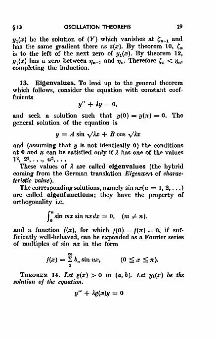
13. Eigenvalues. To lead up to the general theorem which follows, consider the equation with constant coefficients
y" + ).y = o, and seek a solution such that y(O} = y(1r) = 0. The general solution of the equation is
y = A sin -ylh + B cos -ylh
and (assuming that y is not identically 0) the conditions at 0 and 1r can be satisfied only if .A. has one of the values 19, 22, ••• , ns, •••
These values of .A. are called eigenvalues (the hybrid coming from the German translation Eigenwert of characteristic value).
The corresponding solutions, namely sin n.r{n = 1, 2, .•. ) are called eigenfunctions; they have the property of orthogonality i.e.
J: sin m.r sinn.rcl.r = 0, (rn =1= n).
and a function /{.r), for which /{0) = j(1r) = 0, if sufficiently well-behaved, can be expanded as a Fourier series of multiples of sin nx in the form
00
/(.r) = I: b,. sinn.r, 1
(0 ~X:;;;; 1r).
TuEORElt 14. Let g(x) > 0 in (a, b). Let Y.t(X) be the solution of the equation.
y" + lg(x)y = o
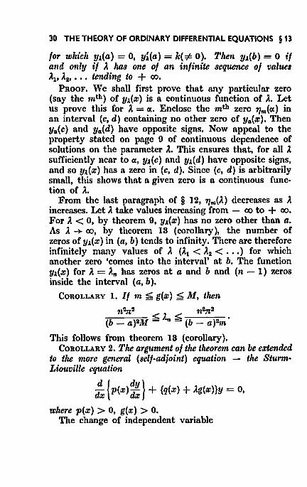
30 THE THEORY OF ORDINARY DIFFERENTIAL EQUATIONS § 13
for which Y.t(a) = 0, yA(a) = k(i= 0). Then Y.t(b) = 0 if and only if A ha8 one of an infinite sequence of values A1, A2, • • • tending to + co.
PROOF. We shall first prove that any particular zero (say the mth) of YA(.x) is a continuous function of )... Let us prove this for A = ot. Enclose the mth zero 17m(«) in an interval (c, d) containing no other zero of Ycx(.x). Then Ycx(c) and Ycx(d) have opposite signs. Now appeal to the property stated on page 9 of continuous dependence of solutions on the parameter A. This ensures that, for all ).. sufficiently ncar toot, Y.l(c) and YA(d) have opposite signs, and so y1(.x) has a zero in (c, d). Since (c, d) is arbitrarily small, this shows that a given zero is a continuous function of i..
From the last paragraph of § 12, 17m().) decreases as A increases. Let A take values increasing from - co to + co. For A< 0, by theorem 9, YA(.x) has no zero other than a. As l -+- co, by theorem 18 (corollary), the number of zeros of YA(.x) in (a, b) tends to infinity. There are therefore infinitely many values of A (..t1 < A2 < ... ) for which another zero 'comes into the interval' at b. The function Yl(.x) for A= A, has zeros at a and b and (n- 1) zeros inside the interval (a, b).
CoROLLARY 1. If m ~ g(.x) ~ M, then
nl!nll n~ll
(b- a)SM ~An~ (b- a)~ This follows from theorem 18 (corollary).
CoROLLARY 2. The argument of the theorem can be extended to the more general (self-adjoint) equation - the SturmLiouville equation
! { p(.x) ~} + {q(.x) + Ag(.x)}y = 0,
where p(.x) > O, g(.x) > o. The change of independent variable
§14 OSCILLATION THEOREMS
f., dt
~- -- a p(t)
transforms the equation into
cJ2y dea + {ql<n + J.gl<eny = o,
to which the methods of the theorem apply.
14. El~enfunctlons and expansions.
31
From the extension of theorem I4 given in corollary 2 we have for the Sturm-Liouville equntion a sequence of eigenvalues .'.1, .l.2, ••• , Ano ••• , and corresponding to An a solution Un(.x), determined except for a constant multiplier, which vanishes at a and band at n - I points inside (a, b). This is called the 11th eigenfunction.
"'e have
(pu:,.)' + (q + .l.,.g)um = 0,
(pu~)' + (q + ).~)Un = 0.
Multiply these equations by Un and u"', subtract, and integrate from a to b. This gives
[p(u:nun - umu~)r + (Am -An) r gumund.x = 0. a a
The expression in square brackets vanishes at a and b, and so, if m =fo n,
The functions ttn(.x) may be said to form an orthogonal set in (a, b) with weight function g(m).
Form = n, we have J: gu~d.x > 0 because the integrand is
positive. The arbitrary multiplier in un may be chosen so as to make the value of the integral equal to I.
31 THE THEORY OF ORDINARY DIFFERENTIAL EQUATIONS § 14
TJIEOREM 15. .All the eigenvalues of the equation
! { p(x):} + {q(x) + Ag(x)}y = o, (a s;; x s;; b),
where p(x) > 0, g(x) > 0, are real. PROOF. Suppose that there is a complex eigenvalue
..t, = tx + i[J. Then, the coefficients of the equation being real, the conjugate complex number is also an eigenvalue, say A. = tx- i[J. Let the eigenfunction corresponding to ..t, be u, = v + iw say. Then u, = v- iw. By the orthogonal property r gu,u,ck = 0,
a which gives
" J g(vS + wS)cJx = o. a
This can only be true if v = w = 0. Thus the theorem is proved.
The eigenfunctions form a basis of expansion of an arbitrary function /(x) for which j(a) = f(b) = 0. Suppose that
f(x) = c1u1(x) + ... + CnUn(X) + ... 1\lultiply by g(x)un(x). If the integration term-by-term from a to b is valid, we have the value of the nth coefficient:
Cn = r g(x)f(x)un(X}dx. a
This expansion is only formal, and the proof of its validity under suitable assumptions about j(x) is beyond · the scope of this book. Justification is immediate if all the un(x) are less than a constant and the uniform convergence of the series is assumed.
Examples of the application of the theorems of this Chapter to special functions will be found in Chapter VIII (Bessel functions).
CHAPTER IV
SOLUTION IN SERIES
15. Differential equations in complex variables. It was remarked in § 1 that few types of differential equations can be solved by a finite number of processes applied to elementary functions, and the work of Chapters II and III will have further impressed this fact on the reader. 'Ve are thus led to investigate solutions which arc expressible by infinite processes, for example, as the sum of an infinite series of elementary functions. A type of infinite series which suggests itself is a power series in x,
00
Y = ~ Cnllln. n-o
Problems of convergence and manipulation of power series are as readily dealt with in complex variables as in real variables, and the question arises whether it is appropriate to widen the scope of our discussion of differential equations and allow the variables to be complex. It is true that in applications to mechanics or physics the reader will have become accustomed to real variables, and it may seem an empty striving after generality to suppose the variables complex.
The reason why this extension is worth while is that differential equations derive much of their importance from the functions which are their solutions. To restrict the variable of a function to be real is to leave out matters of the highest interest e.g. the relation between the exponential and trigonometric functions. In fact, the equation
dw -kw dz- '
33
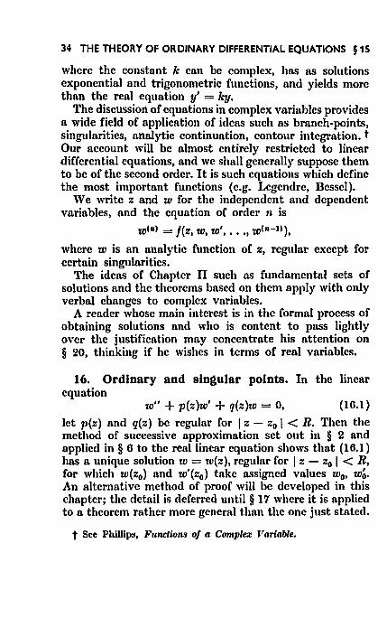
34 THE THEORY OF ORDINARY DIFFERENTIAL EQUATIONS § 15
where the constant k can be complex, has as solutions exponential and trigonometric functions, and yields more than the real equation y' = ky.
The discussion of equations in complex variables provides a wide field of application of ideas such as branch-point'i, singularities, ann.lytic continuation, contour integration. t Our account will be almost entirely restricted to linear differential equations, and we shall generally suppose them to be of the second order. It is such equations which define the most important functions (e.g. Legendre, Bessel).
We write z and w for the independent and dependent variables, and the equation of order n is
WCnl -j(z W w' wCn-11) - J ' , ••• , t
where w is an analytic function of z, regular except for certain singularities.
The ideas of Chapter II such ns fundamental sets of solutions and the theorems based on them apply with only verbal changes to complex variables.
A reader whose main interest is in the formal process of obtaining solutions and who is content to pass lightly over the justification may concentrate his attention on § 20, thinking if he wishes in terms of real variables.
16. Ordinary and sin~ular points. In the linear equation
w" + p(z)w' + q(z)w = 0, (16.1)
let p{z) and q(z) be regular for I z- z0 I < R. Then the method of successive approximation set out in § 2 and applied in § 6 to the real linear equation shows that (16.1) has a unique solution w = ro(z), regular for I z- z0 I < R, for which w(z0 ) and w'(z0 ) take assigned values w0 , w~. An alternative method of proof will be developed in this chapter; the detail is deferred until § 17 where it is applied ton theorem rather more general than the one just stated.
t See Philli~, Functions of a Complea: Variable.
§ 16 SOLUTIONS IN SERIES 35
DEFINITION. A value z = z0 for which the coefficients p(z) and q(z) arc regular is called an ordinary point of the differential equation. All other points are singular points or sin~ularlties of the equation.
If p(z) and q(z) are regular for all finite z, the solutions will be regular for all finite z. For R in the first paragraph can be as large as we like.
If p(z) nnd q(z) have singularities, the solutions will in general have singularities for the values of z concerned.
Example I. w''=%U.".
By the remark just made, solutions will be regular for all finite z, and we may assume expansions in powers of :, t
tv = a0 + a1: + ... + a,.z" + ... Substitute in the equation and equate coefficients of powers of ::. Then
"• = o, n(n - 1 )a .. = a .. _3 , n ~ 3.
So tv= llo { 1 + 2~33 + 2.3~5. 6 + ... )+at{::+ 3~4 + 3 .. ,~76 .7+ ... ). where a0 and a1 are arbitnny eonstnnts (in fnct they nrc the values of rv and w' for :: = 0).
Example 2. l.w
tv'=-· :1;
This hns solutions w = A::•. The origin is in general a branch point (e.g. k = ! ); it may be regular (k = 1) or n pole (k = - 1 ).
Example n. tv
w'=-· :~:•
Solutions are rv = A exp (- 1/:), which have an essential singularity at :: = o.
We remark that the positions of singularities of solutions of a differential equation may or may not depend on the
t Phillips, p. 05.
36 THE THEORY OF ORDINARY DIFFERENTIAL EQUATIONS § 17
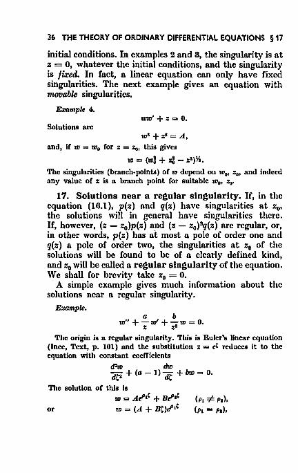
initial conditions. In examples 2 and 8, the singularity is at z = 0, whatever the initial conditions, and the singularity is fixed. In fact, a linear equation can only have fixed singularities. The next example gives an equation with movable singularities.
E3:ample 4. wm' + z = 0.
Solutions arc to1 + zl =A,
and, if w = w0 Cor z = .zo, this gives
w = (wX + Z: - :•)%.
The singularities (branch-points) of w depend on w0 , : 0 , and indeed any value or z is a bmneh point Cor suitable w0, Zo·
17. Solutions near a regular singularity. If, in the equation (16.1 ), p(z) and q(z) have singularities at z0,
the solutions will in general have singularities there. If, however, (z - z0 )p(z) and (z - z0 ) 11q(z) arc regular, or, in other words, p(z) has at most a pole of order one and q(z) a pole of order two, the singularities at z0 of the solutions will be found to be of a clearly defined kind, and z0 will be called a regular singularity of the equation. We shall for brevity take z0 = 0.
A simple example gives much information about the solutions ncar a regular singularity.
EMmple. a b
w" + - w' + - w = 0. :: =' The origin Is a regular singularity. This is Euler's linear equution
(lnee, Text, p. 101) and the substitution : = ~ reduces it to the equation with constant coefficients
tPw dw tJCl +(a- 1) tiC + bw = 0.
The solution or tllis is m = AtftC + Btf.C (p1 =ft. p1),
or w = (A + BC}t!'' (p1 = p1},
§17 SOLUTION IN SERIES
where p1 and p1 arc the roots or the quadmtie
p(p - I) + ap + b = o. So the solutions of the original equation are
w = Az"l + B:.P•
or w = (A + B log :.)z"l in the respective cases of unequal and equal roots.
37
Thus the solutions in geneml are many-valued functions having bmneh-points at ::: = 0, and in the equal-root case, if w1(z) is the solution zP1 immediately given by the root p1, a second solution is w1(z) log:..
Formal calculation of solutions of w" + p(z)w' + q(z)w = 0,
where zp(z) and z2q(z) are regular at z = o. There is a circle, centre z = 0, in which
The first equation gives the quadratic for p F(p) = o.
This is called the indicial equation, and its roots, say p1 and p2 , arc the exponents at the value of z (z = 0) under consideration. The equations after the first give successively the values of c1, ••• , cn, ..• in terms of c0• The equations arc linear, and, for each value of p, the c's are
38 THE THEORY OF ORDINARY DIFFERENTIAL EQUATIONS § 18
uniquely determined unless, for some value of n, the coefficient of Cn in the equation for cn vanishes, that is to say, F(p + n) = 0. If p1 - p2 = n, then p = p1 gives a (formal) solution, but F(p2 + n) = 0 and the process does not, in general, give a solution for p = p2• l\loreover, if p1 = p2, we obtain only one solution. Leaving aside until § 19 the further investigation required when the indicia} equation has equal roots or roots differing by an integer, we establish the convergence of the power series Ec,;;.n which has been found.
18. Conver~ence of the power series. THEOREM 16. With the notation of § 17, suppose that
zp(z) and z2q(z) are regular for I z I < R. Then the series obtained corresponding to a value p satisfying tile indicial equation converges for I z I < R.
PuooF. If the series terminates, this is true; suppose that it is an infinite series. Let p' be the other root of the indicial equation.
We enter upon a majorising argument, replacing every Cn by a number Cn such that I en I :S: Cn.
Let r be any number less than R. By Cauchy's inequality there is a number K = K(r), t independent of n, for which
I Pn I ;;i ~ • I qn I ;;i ~ (n = 0, I, 2,. • .).
The modulus of the right-hand side of (18.1) is then less than or equal to
Kn:Ell c II PI+ s + 1. -o • r" •
t PWllips, Fu11ctions of a Complez Variable, p. DO, Corollary.
SOLUTION IN SERIES 39
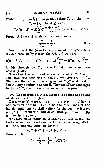
Write 1 p - p' 1 = A., I p 1 = I'• and define C,. by the rules Ca = I c,. I for 0 :5: n < i.,
n-1 p+a+1 Cnn(n- i.) = K ~ C, for n :::;:::: i.. (18.2)
s-o rn-•
From (18.2) we shall show that, as n -+ oo,
C,. -+_!_· {18.8) Cn-1 T
For subtract the (n- 1 )th equation of the type (18.2) divided through by r from the nth and we have
n(n - .l)C,. - (n - 1 )(n - 1 - i.) C,._1 = K(p + n) C,._1, T T
Divide through by C,._1n(n- i.), let n -+ oo and we obtain (18.8).
Therefore the radius of convergence of J: C,.z" is r. But, from the definition of the C,., we have I c,. I ~ C,.. Therefore the radius of convergence of J:c,.z" is at least r. But r is any number less than R. Therefore J:c,.z" converges for I z I < R, and this is what we set out to prove.
19. The second solution when exponents are equal or differ by an inte~er.
Letw = w0(z) = zP(c0 + c1z + ... + c,.z" + ... )be the one solution obtained. Let p' be the other root of the indicia! equation; we shall write v for the positive integer p - p' + 1. From the indicial equation p + p' = 1 - p0,
and so 2p +Po= v. The method of reduction of order (§ 9} will be used to
find a second solution from the known solution w0• Write w = w0v, and the equation for v is
w0v" + {2w~ + p(z )w0}v' = 0, from which
v' = ~ exp{- f'p(C)dC}
40 THE THEORY OF ORDINARY DIFFERENTIAL EQUATIONS § 20
A - liP( + + )ll exp( -p0 log z- p1z- !Pr~- ... ) Z Co c1z •• ,
A - "( + + )ll exp(- PtZ- !PsZ11- ••• ) Z c0 c1z , , ,
A = ZV g(z),
where g(z) is regular at the origin and g(O) = 1/c'f,. In a circle, centre z = 0, g(z) can be expanded in a Taylor series
a0 + a1z + ... , (a0 =I= 0). Integrate v' to obtain v, and we have for the second solution any constant multiple of
w0(z) {- (v _ a;)zv-t- •.• - a:-ll + a.,_1 log z+a..z+. ·l This is
co D 11_ 1w0(z) log z + zP' :E bnZ"· (19.1)
A-D If the roots of the indicial equation are equal, v = 1 and p' = p, and since a0 =1= o, the term in log z is always present.
For roots differing by an integer, it may happen that a.,_1 = 0, and in that case there is no logarithmic term.
20. The method of Frobenius. It will be noticed that in§ 19 there is no means of finding the general term in the expansion of g(z), and so we look for other methods better adapted to giving the general term in the solution. One way would be to substitute the known form (19.1) of the solution in the equation and find the b, by equating coefficients of powers of z. Another method is that of Frobenius (1873), which will now be explained.
Assume as before w = zP(c0 + c1z + ... ).
Let p1 and p2 be the exponents. The equation (17.1) for c11 is
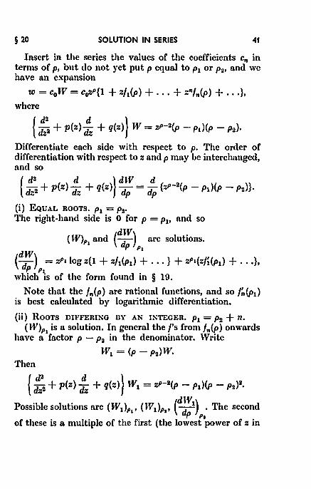
Insert in the series the values of the coefficients en in terms of p, but do not yet put p equal to p1 or p2, and we have an expansion
w = c0W = CoZP{l + zil(p) + ... + z"fn(p) + ... }, where
{ ~: + p(z)! + q(z)} lV = zP-3(p - pd(p - P:~)· Differentiate each side with respect to p. The order of differentiation with respect to z and p may be interchanged, and so
Possible solutions are (W1 )p1 , (W1 )p1, (ddlV1} • The second
P Pa of these is a multiple of the first (the lowest power of z in
42 THE THEORY OF ORDINARY DIFFERENTIAL EQUATIONS § 2.1
each is z/'1 }, and the third is the solution we are seeking. For an example in which there is a factor p-p9 in the
numerator of fn(P} cancelling the one in the denominator, so that the solution with exponent Pais valid, see §22 (iii).
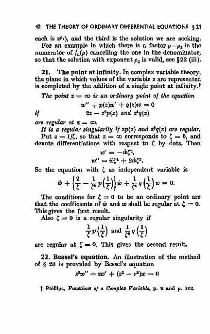
21. The point at infinity. In complex variable theory, the plane in which values of the variable z are represented is completed by the addition of a single point at infinity.t
The point z = oo u an ordinary point of the equation w" + p(z)w' + q(z)w = 0
if 2z - z2p(z} and z'q(z}
are regular at z = oo. It is a regular singularity if zp(z} and z9q(z} are regular. Put z = 1/l;, so that z = oo corresponds to C = 0, and
denote differentiations with respect to C by dots. Then w' = -wca.
w" = wC' + 2wc:'. So the equation with C as independent variable is
.. { 2 1 ( 1 )} . 1 ( 1 ) w + C - CS P C w + C' q C w = o. The conditions for C = 0 to be an ordinary point are
that the coefficients of w and w shall be regular at C = 0. This gives the first result.
Also C = 0 is a regular singularity if
~ p { ~) and ~8 q { ~) are regular at C = 0, This gives the second result.
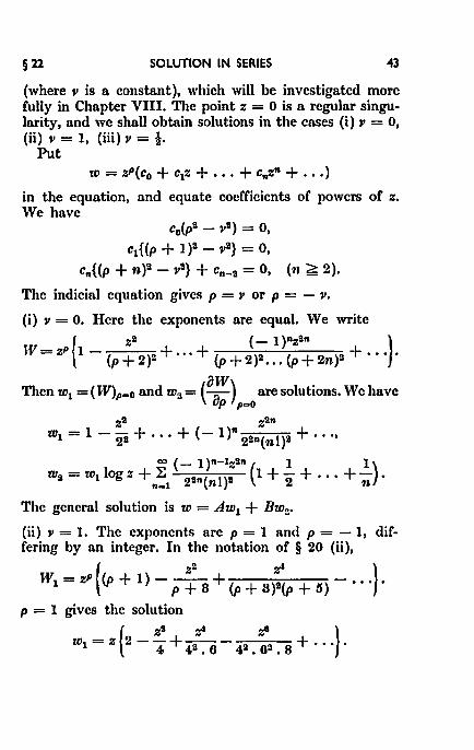
22. Bessel's equation. An illustration of the method of § 20 is provided by Bessel's equation
z'Lro" + zw' + (zll - v2)w = 0
t Phillips, Functions of a Complez Variable, p. 9 and p. 102.
§22 SOLUTION IN SERIES 43
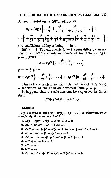
(where v is a constant), which will be investigated more fully in Chapter VIII. The point z = 0 is a regular singularity, and we shall obtain solutions in the cases (i) v = O, (ii) v = I, (iii) v = l·
Put w = zP(c0 + c1z + ... + c,.z" + ... )
in the equation, and equate coefficients of powers of z. We have
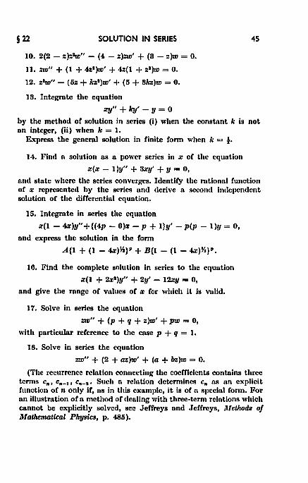
by the method of solution in series (i) when the constant k is not an integer, (ii) when k = 1.
Express the general solution in finite form when k = !·
14. Find a solution as a power series in z of the equntion
z(z- l)y" + 8xy' + y = 0,
and state where the series converges. Identify the ratlonnl function of z represented by the series and derive a second independent solution of the differential cquntion.
15. Integrate in series the equation
x(1- 4z)y"+{(4p- 6)z- p + I}y'- p(p- 1)y = o,
and express the solution in the form
A{I + (I - u)Y.}P + B{1 - (1 - .J.r)Y.}P.
16. Find the complete solution in series to the equation
x(l + 2z1)y" + 2y' - 12:ry = 0,
and give the range of vulucs of z for which it is valid.
17. Solve in series the equation
::w" + (p + q + ::)w' + pw = 0,
with particular reference to the case p + q = 1.
18. Solve in series the equation
:w" + (2 + a:)w' + (a + b:)w = 0.
(The recurrence rclution connecting the coefficients contains three terms c,., c,._1 , Cn-t• Such a rclution determines c., as un explicit function of n only if, us In this example, it is of u speclnl form. For un illustration of a method of dealing with three-term relations which cannot be explicitly solved, see Jeffreys and Jeffreys, lllelhods of Mathematical Physics, p. 485).
46 THE THEORY OF ORDINARY DIFFERENTIAL EQUATIONS § ll
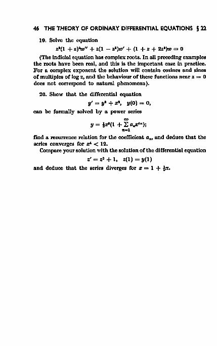
19. Solve the equntion
z1(1 + :)lm" + :(1 - : 1)10' + (1 + : + 2zl)w = o (The indicial equation has complex roots. In all preceding exnmples
the roots have been real, and this is the important ease In pmctlce. For a complex exponent the solution will contain cosines and sines of multiples or log :, and Ute behaviour or these functions ncar z = 0 does not correspond to natuml phenomena).
20. Show Utnt the differential equation
y' = Y' + m', y(O) = 0,
can be formally sol\'ed by a power series co
y = Ja:l(l + ~ a~n); n-1
find a recurrence relation for the coefficient a0 , and deduce that the series converges for~< 12.
Compare your solution with the solution or the differential equation
:' = : 1 + 1, :(1) = y(1)
and deduce Utnt the series dl\'erges for z = 1 + J\n.
CIIAPTER V
SINGULARITIES OF EQUATIONS
23. Solutions near a sln~ularlty. In Chapter IV solutions in the form of infinite series were obtained near a regular singularity of a differential equation. The following discussion throws further light on the distinction between regular and irregular singularities.
In the equation
w" + p(z)w' + q(z)w = 0,
we suppose that z = 0 is a singularity of one or both of p(z) and q(z) and that there is a circleS with centre z = 0 in which they are one-valued and have no other singularities. If z0 is any point (not 0) inside S, there are two linearly independent solutions of the equation
w" + p(z)w' + q(z)w = 0,
say w1(z) and w2(z), regular in a circle centre z0 • These solutions have analytic continuations along a path in S enclosing the origin and returning to z0 • Let the functions so obtained as the continuations of w1(z) and w2(z) be W1(z) and W2(z) respectively.
The functions obtained at each step of the process of continuation satisfy the differential equation, and any solution is the sum of constant multiples of the functions of a fundamental set. Therefore
W1(z) = aw1(z) + bw11(z) W:~(z) = cw1(z) + dw2(z)
where ad- be=#= o. (If ad= be, then cW1(z)-aW11(z) = 0, and so, carrying out the analytic continuation in the
67
48 THE THEORY OF ORDINARY DIFFERENTIAL EQUATIONS § 23
opposite direction along the path, cw1(:~)- aw2{z) = 0 which contradicts the linear independence of w1 and w8.)
We now find the condition that a solution when continued round z = 0 is unaltered except for a constant multiplier.
Any solution w, regular at z0, can be expressed as
tX'W1 + Pwa• By continuation round z = 0 this becomes
cx(aw1 + bw2 ) + p(cw1 + dw2).
This expression is of the form ).(cxw1 + pw2) if
cx(a - ).) + pc = O,
and cxb + p(d- .t) = 0;
. , . r Ia-). c I 1.e. ,. must satts y b d _ ). = 0. (28.1)
CAsE (i) UNEQUAL ROOTS ).1, ).2•
We can take a new fundamental set of solutions at z0,
calling w1(z) the solution which acquires the multiplier ).1,
and w2(z) that which acquires the multiplier A:~~• The function zP acquires a multiplier eS"'P in going
round z = 0. So, if 2nip1 = log ).1 and 2nip2 = log J.a, then :rP1w1(z) and :rPaw2(z) are single-valued in S and can be expanded in Laurent series. So we have the canonical fundamental set of solutions near the singularity %=0
co co w1(z) = %1'1 l: a,.n, w2(z) = zP•l: b,_n, {28.2)
-co -co
CASE (ii) EQUAL ROOTS ).1,
There is, as in case (i), a solution w1 whose continuation is W1 = ).1w1• Suppose that W2 is the continuation of cw1 + dw8• Then the equation corresponding to {28.1)
I ;.. - ). c I = 0 0 d-).
§ 24 SINGULARITIES OF EQUATIONS
has equal roots A = Ar So d = A1 and
H'2 =toll+.!:..., wl wl A.l
49
that is to say, w2fw1 is increased by cfA.1 when z goes round the origin. Therefore
Wa __ c_logz w1 2niA1
is single-valued in S and can be expanded in a Laurent series. This gives for the canonical fundamental set in the equal-root case
00
w1(z) = zPt ~ anzn, -oo
00
w2(z) = zP, ~ bnZn + kw1(z) log z. -oo
(28.8)
24. Regular and irregular singularities. The process set out in § 28 of investigating solutions which acquire a constant multiplier by analytic continuation round a singularity is not a practical one for the calculation of coefficients in the solutions, and we must think of ways of finding the an and bn in the canonical forms. The most
00
natural is to assume w = zP ~ anzn, substitute in the -co
differential equation and equate coefficients of powers of z. If we do this (on the lines of § 17) it is apparent that the Laurent series will give rise to equations containing infinitely many unknowns, and they arc manageable only if the Laurent series contain finitely many negative powers. It is this case which is singled out as a regular singularity. The best definition is now seen to be the following.
DEFINITION. An isolated singularity z =a of a differential equation is called regular if there is a constant k such that, for every solution w(z),
(z- a)tw(z) ~ 0 as z ~a.
SO THE THEORY Of ORDINARY DIFFERENTIAL EQUATIONS § 24
The singularity is called irregular if it is not regular. It is clear that, if the Laurent series have only finitely
many negative powers, the singularity is regular according to the definition. The converse is true. For, choosing k to be m - p1 where tn is a integer, we have for w1, co :E a.a(z- a)n -+0 as 2 -+a, from which an= 0 for n ;S; 0.
-co A similar remark holds for w8•
The next theorem shows that the definition of regular singularity just given accords with the usage of Chapter IV. We again take a = 0 for brevity.
THEOREM 17. Necessary and sufficient conditiom for z = 0 to be a regular singularity oj the equation
w" + p(z)w' + q(z)w = 0
are that zp(2) and z11q(z) are regular at 2 = 0 (at least one oj p(z) and q(z) having a singularity there).
PROOF. The sufficiency has already been established by the finding of the solutions in §§ 17- 19. We prove the necessity.
where Pll = p1 if k =1:- O, and in which the Laurent series have finitely many negative powers.
Since w1 and w11 satisfy the differential equation, we have
(z) = _ W1~'- w.l'w2 = _ .!!...[]o {w11 !:.._ {Wz) }] p W1W~ - wl'W11 dz g 1 dz W 1
§25 SINGULARITIES OF EQUATIONS 51
w ()() Now 2 = k log z + zPa-Pa+m .t CnZ", where m is an
Wt 0 integer, c0 =F 0, and p2 = Pt if k =I= 0. Consequently,
.!!_(tea) = k + zPa-Pa+m-t ~ dnz", dz Wt Z o
~ {Wu) = - .!:_ + zPa-Pa+m-2 ~ e z". dz2 tOt zll o n
The quotient of the last expression by the preceding is regular or has a pole of order one at z = 0; the same is true of w~fw1, and therefore of p(z}.
Since Wt satisfies the given differential equation, we have
w1' ~ q(z} = ---p(z}-· tOt tOt
Since w;jw1, w!' fw; and p(:::} are regular or have poles of order one, therefore q(z} is regular or has a pole of order one or two. This proves the theorem.
25. Equations with assigned singularities. In this section we admit only second-order differential equations whose singularities for finite z or for z = co arc regular. t
There is at least one finite value of z for which such an equation has a singularity, unless the equation is w" = 0.
For an equation with no singularity for a finite z is of the form
w" + p(z)w' + q(z)w = 0,
where p(z} and q(z} are regular for all finite z. But unless p(z} = q(z} = 0, the singularity for z = co is irregular.
An equation whose only finite singularity is at z = a is of the form
"+ b , c (b ) w --w + ( }:tw = O, , c constants. z-a z-a This equation has a singularity at z =co. unless b = 2, c = 0.
t See §§ 16, 17, 21.
52 THE THEORY OF ORDINARY DIFFERENTIAL EQUATIONS § 16
For the general equation with a singularity at a is
w" + p(.z) w' + q(.z) w = 0, 2- a (2- a)2
where p(.z) and q(.z) are regular for all finite z. From § 21, the singularity at 2 = co can only be regular
if p(2) and q(2) are constants. From § 21 again, the conditions for 2 = co to be an ordinary point are b = 2, c = 0, in which case the equation integrates to
A W=--+B. z-a Equation wit/~ two singularities. If the singularities are
at 2 = a, 2 = b, while z = oo is an ordinary point, we can reduce this ease to the last by the transformation C = (.z- a)/(2- b), which gives an equation inC with 0 and co as singularities.
26. The hypergeometric equation. We next consider equations with three regular singularities. Any three points can be transformed by a bilinear substitution into 0, 1, co. t We shall obtain a standard form of equation having singularities at 0, 1, oo.
Take the equation w" + p(z)w' + q(2)rv = 0.
Then z(1 - 2)p(2) and 211(1 - z)9q(z) are regular for all finite 2 and zp(z), .zllq(z) are regular for z = co. So the most general forms of p(z) and q(z) are
p(z) =Po+ P1Z, q(z) = qo + qlz + q'l!-9,
z(1 - z) zB(1 - 2):1
We may, by a change of dependent variable w = ZCX(1 - z)l' W,
suppose that for each of the values z = 0 and z = 1 one of the two exponents is zero.
t Phillips, Furn:tions of a Comple:t Varillble, p. 40.
§ 27 SINGULARITIES OF EQUATIONS 53
If, then, W = c0 + c1z + , , , , (Co =/= 0)
satisfies the equation, we find by substituting in the equation that q0 = 0, so that z is a factor of the numerator of q(z ). So, for the same reason, is l - z. The equation is now reduced to
z{1 - z)w" + (p0 + p1z)w' + q1w = 0.
The coefficients p0 , p1, q1 are most conveniently expressed in terms of the exponents at z = oo, and the exponent other than zero at z = 0, Let the exponents at oo be a, b.
Putting
1 ( c1 ) W=- c0 +-+••• zP z
we find the indicia) equation at oo to be
- p(p + 1) - PtP + ql = 0.
If the roots are a, b, then
ab = - q1, a + b = - p1 - I.
The final form of the equation is
z{1- z)w" + {c- (a+ b + 1)z}w'- abw = 0, {26.1)
where the remaining exponent at z = 0 is 1 - c. This is the bypergeometric equation.
27. The bypergeometric function. Solutions of (26.1) near z = 0 arc given by
w =zP(c0 + c1z +,,, + c,.zn +,, .). 'Ve know already that p = 0 or 1 -c. The recurrence relation is found to be
{p + n + a )(p + n + b) c,.+l = (p + n + 1){p + n + c)c,..
54 THE THEORY OF ORDINARY DIFFERENTIAL EQUATIONS § 28
If c is not a negative integer, p = 0 gives the solution
This series will be called F(a, b; c; z), the hypergeometrlc function. The radius of convergence of the series is found to be 1; this could also be predicted from the fact that the singu]arity nearest to 21 = 0 is z = 1.
The second solution near z = 0 is
z1-cF(a - c + 1, b - c + 1; 2 - c; z),
on the assumption that c is not an integer. In further work with hypergeometric functions, we shall assume that the exponents at any singularity under consideration do not differ by zero or an integer.
With three parameters a, b, c at our disposal, it is easy to fit many common functions into hypergeometric form, for example
This gives (28.1). The right-hand side of (28.1) is a regular function of z in the whole plane, cut along the real axis from 1 to + co. This provides the analytic continuation of F(a, b; c; z) outside the circle I z I < 1 in which it was defined by the series.
29. Formulae connecting hypergeometric functions. There are vast numbers of relations connecting hypergeometric functions with different parameters, and we give only a few, choosing those which rest on interesting work in convergence or manipulation of gamma-functions. We prove first
THEOREM 19. If R(c- a- b) > 0, the series for F(a, b; c; 1) converges and
F(c)r(c- a- b) F(a, b; c; 1) = F(c- a)r(c- b)•
t Gillespie, lntegratUm, § 88.
56 THE THEORY OF ORDINARY DIFFERENTIAL EQUATIONS § 29
PnooF. If Un is the nth term in the series for F(a, b; c; 1 ),
Un =(1+n)(c+n)= 1 +c-a-b+1 o(~)· Un+1 (a + n)(b + n) n + nil
Convergence is shown by Gauss's test. Then, from Abel's limit theorem, t
F(a, b; c; 1) =lim F(a, b; c; a:) = ... 1-0
=~~r(b 9~1-b) J:tb-1(1-t)c-b-l(1-a:t)-a dt, from {28.1)
- r{c) J1 .111-1( )c--o-6-ldt - F(b)F(c-b) o ,- 1 - t '
since this last integral exists, and (1 - a:t)-<~ -+ (1 - t)-<~ uniformly for 0 ~ t ~ 1 if Ra ~ 0, whereas, if Ra > O,
I (1 - a:t)-<~ I ~ I {1 - t)-<~ I in which case Weierstrass's M-test for integrals applies. Since
J1 F(b)r(c - a - b) t}l-1(1 - t)C-<1-b-ldt = ,
o F(c- a) we have the result.
This method of proof is subject to the limitation of § 28 that Rc > Rb > 0. The result, however, is true independently of this.
Finally we prove a formula connecting hypergeometric functions of z and 1 - z.
The solutions convergent for I z I < I are F(a, b; c; z), (i)
zt-cF(a- c + 1, b- c + 1; 2- c; z). (ii) If we write z = 1 - C in the hypergeometric equation (26.1 ), it becomes
d'lw dm C(1-C) flC3 +{(a+b-c+1)-(a+b+1)C} dC -abm = 0.
t For the 0-notation, Gauss's test. and Abel's theorem, sec Hyslop, Infinite Series, pp. 14, 40, 80.
§ 30 SINGULARITIES OF EQUATIONS 57
Writing down the solutions of this equation valid for I C I < I and replacing C by I - z, we have
F(a, b; a+ b- c +I; 1 - z), (iii) (I - z)c-a-IIJ•'(c- b, c- a; c-a-b+ 1; I - z). (iv)
The functions (i )-(iv) are solutions of the hypergcometric equation in the domain common to the circles I z I < 1, li-z I < 1. There must be two linear identities connecting them. One of these is
(i) = A(iii) + B(iv). We shall obtain the constants A, B. Let z -+ 1 along the real axis. We have
Mter some manipulation we can deduce that B = F(c)F(a+b-c).
F(a)F(b)
30. Confluence of sin~ularities. The function & is not of the form F(a, b; c; z). It can,
however, easily be shown to be lim F(a, b; a; zfb ). 11-+00
The equation of which F(a, b; c; zJb) is a solution is
( z) , ( a+ 1 ) , z 1 - b w + c- z - -b- z w - aw = o.
This has regular singularities at 0, b, co. When b -+ co, we have the confluence of the two singularities b, co. The equation then becomes
zw" + (c - z)w' - aw = 0,
with a regular singularity at z = 0 and a singularity at co that is easily seen to be irregular.
58 THE THEORY OF ORDINARY DIFFERENTIAL EQUATIONS § 30
Information about solutions of this last equation is more easily obtained directly than by limiting operations on hypergeometric functions.
E:ramples.
1. Prove that the solutions of
::w" - (1 + z)w' + w = 0
in powers or z are regular at :: = 0. A value such as :: = 0 in tllis equation which, according to the
definition, is a singularity or the equation but at which t11e solutions are regular may be called an apparent singularity.
2. For the equation
:'w" + (1 + :)w' - aw = o, which bas an irregular singularity at z = o, prove tllat, in general t11cre is no solution or t11e Corm zl'r(z), where r(::) is regular at :: = 0; if, however, a is the square or an integer there is one such solution. Obtain this solution when a = 4.
B. Prove that the equation
z'w" + z'w' + w = 0
has no solution zl'r(::), where r(:) is regular at z = 0. Prove that z = oo Is a regular singularity of the equation. 4. Prove that there Is a solution of the equation
:a(1 + z)w" + :(1 + 2:)w' - (1 + 2:)w = 0
regular at : = 0. Find also a solution regular at::= oo, and write down the general
solution of the equation.
5. Prove that, if I z I < 1,
fn/9 d(J
o ..; {1 -:: sin1 0} = lnF(!, !; 1; ::).
6. Prove that, ira- b is not an integer, the general solution or the hypergeometrie equation In powers of 1/z is
31. Solutions expressed as integrals. Because solutions of a differential equation cannot in general be expressed as a finite combination of elementary functions, we were led in Chapter IV to investigate solutions expressed as infinite series of such functions (powers of z - a). Another common way of carrying out a limiting process on elementary functions is by integration with respect to a parameter e.g.
tp(x) = r f(x, t)dt 4
In this chapter we shall set out to find solutions of differential equations in this form.
The solution will be most manageable if it is the integral of a real function with respect to a real variable, but there are advantages in discussing the problem on the wider basis of complex function-theory and seeking solutions
w = f c /(z, C)dC,
where C is a contour in the C-plane. \Ve make one remark here to save constant repetition
throughout the chapter. \Yhen an integrand contains a function such as (C - a)~<, which is many-valued, it is to be understood that one of its values is fixed for a suitnble value of C, and that this chosen branch of the function is followed along the contour of integration.
60
60 THE THEORY OF ORDINARY DIFFERENTIAL EQUATIONS § 32
32. Laplace's linear equation. As an example of an equation whose solutions arc conveniently expressed as complex integrals, we take the nth order equation
in which the coefficients of w and its derivatives are of the first degree in z. This equation in real variables is discussed by !nee, Text, p. 104.
Try to solve the equation by
w = fc e•CP(C)~ for a suitable choice of the function P(C) and the contour C. It will be seen in the light of experience why this is a hopeful trial solution. Substitute for w and its derivatives in the equation. We assume that P(C) and Care such that the derivatives are given by differentiating with respect to z under the sign of integration.
Before embarking on a general discussion of the choice of contours it will be helpful to consider an illustrative example.
Eommple. :ml' + (p + q + z)w' +pro = 0.
Take w = Jce''P(C)tJC. The reader is advised to carry through
the detail for bimsclr, and he will rind that
fc~CH(C + I)HtJC
is a solution if [e•tcp<C + I)'lc = o.
It is convenient to replace C by - C, and then
Jce-•'cP-l(I - C)HtJC
is a solution it [e-•CCP(l - C)']c = o.
Suppose for simplicity that z, p, q arc real. Ir p > 0 or q > O, the intcgmted part in square brnckcts vanishes at C = 0 or C = I respectively. Ir z > 0 or :: < O, it vanishes at C = oo or C = - oo respectively. \Ve arrive thus at solutions of the equation, or which the following are typical, where C is the interval of the rcnl axis specified.
If p > 0, q > 0, C is (0, 1 ); p > 0, z < 0, C is (- oo, 0).
If p < 0, q < 0, :t < 0, no single segment of the real nxis meets
62 THE THEORY OF ORDINARY DIFFERENTIAL EQUATIONS § 33
the requirements Cor C, but we can take o contour composed of the port or the real axis Crom - co to - 15, then o circle of rndius (j and centre the origin, und then returning from - IJ to - co.
These indications do not profe88 to give the complete solution of the example, but they lend up to the next section.
33. Choice of contours. In the general case of § 82, there arc various possible types of contour C. The condition [fP(C)Jc = 0 is satisfied if C is closed and fP(C) returns to its initial value after describing it. In this case, C must contain at least one of the points ex,. inside it, for if not it would give only the trivial solution w = 0. Another possibility is to make C go to infinity in one or more directions for which fP(C} -+ 0; as fP(C) depends on z, these directions will depend on the values of z.
When C goes round the point cx1 counter-clockwise the power (C - cx1)k1 is multiplied by e2'Zft1• We can therefore define a C for which [fP(C)Jc = 0 by taking a loop round each of cx1 and «:a twice in opposite directions (a doubleloop contour), as shown in the figure.
Fig. 1.
For clearness in the diagram, the parts of the contour are drawn out separately; they can in fact be circles described twice round «1 and «a together with segments of the line joining them. By taking double-loop contours round cx1 and each of «2, ••• , «,. in turn we obtain n - 1 independent solutions of the equation and these solutions have the advantage of being valid for all values of z.
These n - 1 solutions may be expected to be independent; a general formal proof of independence (e.g. by the
§34 CONTOUR INTEGRAL SOLUTIONS 63
Wronskian criterion of§ 7) would be formidable. If it is possible to deform one contour cl continuously into another C2 without passing over any of the points ex1,
then integrals along cl and c'i! yield the same solution of the differential equation; if such a deformation is not possible, the values of the integrals arc in general different. The reader will sec that it is impossible to deform one of the double-loop contours defined in the last paragraph into another without passing over points ex1•
To construct an nth independent solution of the equation valid for given values of z, choose a direction in the 4, plane for which the real part of (z + k0 )C is negative, and take as the contour of integration, say, one coming from infinity in that direction, encircling ex1 (and no other ex) and returning to infinity in the same direction. (Fig. 2)
Fig. 2.
It is possible to define each of the n solutions by a contour of this type instead of taking n- I double-loop contours and only one of this type.
34. Further examples of contours. General principles governing choice of contours have been laid down in § 88. Some details have still to be clarified - for instance, we have still to show how to find n independent solutions when the ex's arc not all different. The procedure to be followed will be seen more readily from a study of particular examples than from description in general terms. As a first example it is instructive to see how the technique of § 82 would yield the known solution of the linear equation with constant coefficients.
64 THE THEORY OF ORDINARY DIFFERENTIAL EQUATIONS § 34
E:mmple 1.
bAwiAI + ... + b1w' + b0ro = 0.
We lind that Jc ~tP(C)t¢ is a solution if
f c ~t P(C)R(C)~ = o,
where R(C) = bAC" + ... + b1C + b0•
Suppose that (C - /1)' is a factor or R(C). Then
f c ~ P(C)R(C)dC = o
iC Ar A 1
P(C) = <C - /1)' + ... + c - p + p(C),
where p(C) is regular at C = fJ, and Cis a contour enclosing fJ and no other zero or R(C).
From Cauchy's Integral formula,
fc ~CP(C)~ = e=fl(B,_,::-1 + ... + Bo),
where the B's are constants. This gives the r independent solutions corresponding to the r·fold root fl.
The next example shows that a double-loop contour encircling two branch-points of P(C) may sometimes be replaced by a simpler contour - a figure-of-eight going round the two points in opposite directions.
This condition is satisfied if C is a figure-of-eight contour, one loop containing C = i and the other C = - i, since the factors exp (± 2ni (v + !)} acquired respectively by (C -i)'*! and (C + if+l cancel. (We are supposing that v has not one or the values 1. f, &, ••• , which would give ro = 0}.
§34 CONTOUR INTEGRAL SOLUTIONS 65
In this example, the result is simplified if we change the variable C to it, so as to trnnsform ± i into ± 1.
Then w = Jce111(1 - P)r-idt is a solution, with the following ns
possible choices or c. (i) if v > - !. the strnight line from - 1 to + 1,
and, if v has not one of the values !. f, & •••• , (ii) a figure-of-eight round - 1 and + 1, (iii) if:: is real and positive, a contour coming from and returning
to infinity along the positive imaginary axis and going round - 1 and + 1.
The next example illustrates contours going to infinity in different directions.
E:xample 3. w'' =%t.V.
(This hns been solved in series as Example 1 of § 16). The sub·
stitution w = Jce•CP(C)~ gives P(C) = e-lC", where C has to
satisfy
[p(C)]c = [e=C-!C"Jc = o. Now (whatever the value of::), tp(C)-+- 0 as C tends to infinity \\ith its
amplitude lying within any of three sectors, namely (- i• ~). {i• 5;).
[ (-i• -~"f) J or 8 1, 8 1 , 8 3 say. So we can take as contours C giving
independent solutionK, e.g. (i) one coming from infinity in 8 1 and going to infinity in 8 1, (ii) one coming from infinity in 8 1 and going to infinity in sl.
35. Integrals containin~ a power of 1; - z. The feature of Laplace's linear equation (82.1) which
suits it to solution by integrals of which the 'kernel' is e=C is the linearity in z of the coefficient of each w<r>; the integrand resulting from substitution in the given differential equation is an exact first dcrivntive of n function e:CS(l;) and the differential equation determining 8(1;) is of the first order. If the coefficients of wlrl are polynomials
66 THE THEORY OF ORDINARY DIFFERENTIAL EQUATIONS § 35
of degree m, then we should have to try to express the integrand as an m-th derivative, and the ensuing differential equation for S((;) is of order m, and it may not be easier to solve than the original equation.
It is natural to ask whether contour integrals having kernels of other than exponential form may be of service in solving differential equations. One other useful form is
Jc<C- z)A+1P(C)d(;, (85.1)
where A. is a constant to be chosen. We shall show that this form is appropriate to an equation in which the coefficient of w<rl is a polynomial of degree r in z. We shall give the detail for the second-order equation
q(z)w" + l(z)w' + kw = 0, (85.2)
q(z) being quadratic in z, l(z) linear and k a constant. First we write equation (85.2) in the form
This is possible because comparison of the coefficients of w' and w in (85.2) and (85.8) determines A. and the linear function r(z). (For the detail see Example, p. 67).
The equation (85.8) is satisfied by the integral (85.1) if
J cP((;){i.(C -z)A-1q(C)+((; -z)1r(C)}dC = o. The integrand is
if and
d - {S(C)(C - z)1} dC S(C) = P(C)q(C)
S'(C) = P((;)r((;).
§35 CONTOUR INTEGRAL SOLUTIONS 67
So S(C) can be found from
S'(C) = r(C) = ~ + ~. S(C) q(C) C - «1 C - tx11
We thus find that
w = Jc<C- tx.)i,-1(C- cx~)ta-1(C- z).t+ldC
is a solution of the equation (85.2) if C is chosen so that
[(C - cx1 )"1(C - cx2 )"a(C - z).l]c = 0.
The contour C is to be chosen by the principles developed in § 88.
E:wmple.
Apply the above method to the hypergeometric cqm1tion (26.1)
::(1 - z)w" + {c- (a+ b + 1)z}w'- abw = o. With the notation of the general discussion, we have
q(z) = z(1 - z),
l(l - 2::) + r(z) = (a + b + l)z - c, !l(l +I)(- 2) + (..t + 1)r'(z) = - ab
Eliminating r(z), we find ..t = -a - 1 or ..t = - b- 1. Taking ..t = -a- 1, we find r(z) =(a- c + 1)- (a- b + 1)z. So
S'(C) r(C) a - c + 1 c - b S(C) = q(C) = C - 1 - C
and we have the solution
w = Jcco-•(1 - C)H-1(C- z)-adC, {35.4)
where C is such tlmt
[C"-<+'(1 - C>·-~<c - z)-"-'lc = o. C cnn nlwnyll be taken to be 11 double-loop contour round C = 0 and C = 1 or round C = 0 and C = z, unless the values or a, b, c nrc such 118 to nllow a llimpler type or contour.
The second value A = - b - 1 gives a contour Integral solution got by lnterciUIIIging a and b In (85.4).
68 THE THEORY OF ORDINARY DIFFERENTIAL EQUATIONS § 35
II in (85.4) we put C = 1/q, we obtain
W = f fj&-1(1 - fj)H-1(1 - Z1J)-Od1J
along an appropriate contour. When Rc > Rb > 0, this integral can be taken along the segment (0, 1) or the real axis, and this is the expression already found in § 28.
E:ramples. 1. Find a solution of the differential equation
w" - 2zw' + 2/aD = o (k ;;;:; 0)
of the form JcebC:f(C)cJC, describing two possible types of contour C.
Show that, if k is a positive integer, there is a solution of the form
tP H.(::)= (-1)•e:-• ch'e-••.
2. For the equation of example 1, obtain also solutions
f e••c c-t-ik(1 - C>-!+l"cJC, z f e=•c c-!-!k(1 - C>l"tiC
along appropriate contours.
8. Find solutions In series of the differential equation
y" - 'J.ry' + 2Ay = 0.
Investigate also solutions of the Corm fceb1u(l)dt, where Cis a
suitable contour. Show in particular that, if). < O, two solutions are
Jeo e-11+9~~:1 t-A-1 dl and Jeo e-ll+lh:l t-l-1 dl o -eo
and recover the solutions in series from these.
4. Prove that the differential equation
::w" + 2aw' - zw = o, where a Is a real constant, may be satisfied by taking
m = Jc<P- 1)-te••dl,
where C Is a suitable contour. Show, in particular, that possible forms of contour are
§35 CONTOUR INTEGRAL SOLUTIONS 69
(I) a figure or eight encircling the points t = 1 and t = - 1 in opposite directions;
(ii) a path coming along the negative real axis from - oo and returning to - oo along Ute negative real axis after encircling Ute point t = - 1, provided Ulat R: > 0;
(iii) Ute real axis from t = - 1 to t = 1, provided that a> 0; (iv) the real axis from - oo to - 1, provided that a > 0 and
R:> o. Show that, when the stated conditions arc satisfied, the solution
given by (ii) is a constant multiple of that given by (iv). Verity that, when a = 0, the contours (i) and (ii) give two linearly independent solutions.
5, Show Uiat Ute equation
Dny- :zy = 0
is satisfied by
11 = r~o A,wr J0
00
exp {w•n - n':'1} dt,
n where co= exp {2ni/(n + 1)} and ~A,= 0.
r-o 6. Prove that the equation
::w"+cw'-w=O
has solutions of the form
zl-c I e=C+l/t c-c cJC,
specifying the appropriate contours.
7. Obtain the complete solution in contour integrals of the equation
zw"' + w = 0.
Examples 1, 4, 7, 18 of Chapter IV arc also suitable for solution by contour integrals.
CHAPTER VII
LEGENDRE FUNCTIONS
36. Genesis of Le11endre's equation. Many problems of mathematical physics involve the finding of a function V which satisfies Laplace's equation
aav + a:av + aav = 0 (;l:z:S aya oz'l.
and also satisfies certain boundary conditions (for example, if V is electrostatic potential, it is constant on the surface of a conductor). Any simplifying feature of the problem specialises the form of solution of Laplace's equation that has to be found. We shall suppose in what follows that there is symmetry about a line, which is taken to be the z-axis.
Laplace's equation transformed to spherical polar coordinates
is
:z: = r sin 0 cos rp, y = r sin 0 sin rp, z = r cos 0
asv _! 8V ..!:_ asv + cot08V + 1 811V _0 or9 + r or+ r9 802 r2 80 r11 sin11 0 orp" - •
We are then interested in solutions which are independent of rp. Putting V = rne, where f?J is a function of 0 only, so that V is homogeneous and of degree n, we find
dlf?J de dOS + cotO dO + n(n + 1)@ = o,
or, changing the independent variable to p. = cos 0,
tiSe de (1 - p.9 ) dp.s- 2p. dp. + n(n + 1}9 = 0,
70
§37 LEGENDRE FUNCTIONS 71
a second-order equation for 8 as a function of I'· This is Legendre's equation.
In physical applications e and p. arc real and -I ~p~I. In investigating the functions which are defined as solutions of the equation, we get a more comprehensive picture if the variables are complex, and we replace e, p, by w, z, obtaining
(I - z2 )w"- 2zw' + n(n + I}w = 0, (86.1)
an equation with regular singularities at - 1, I, oo.
37. Legendre polynomials. It will be shown that, if n is a positive integer or zero, Legendre's equation (86.I) has a polynomial solution of degree n. The coefficients of powers of z in the polynomial are found most readily if we solve in series of powers of 1/z. Write
I ( c1 c, ) w = -P c0 + - + •.. + - + • . . • z z z'
Substituting in the equation and equating coefficients of z-P, we have the indicia! equation
- p(p + I) + 2p + n(n + 1) = 0,
giving p = n + 1 or p = - n. We obtain the recurrence relation
c,(p + r + n)(p + r- n -1) = c,_2(p + r- I)(p + r- 2).
The exponent p = - n gives the solution
=Azn{I- n(n-1) _11+n(n-I)(n-2)(n-8) -4 _ }
w 2(2n-1} 2 2. 4(2n-1)(2n-8} z .. · '
This is a polynomial of degree n. We define P 11(z) to be the value of w when
(2n)l A= 2n(nl)1 '
72 THE THEORY OF ORDINARY DIFFERENTIAL EQUATIONS § 38
so that 1 " (-l)r(2n-2r)l P (z) = - I: zn-llr
" 2",...0 rl(n-r)l(n-2r)! ' (87.1)
where p is !nor !(n- 1) according as n is even or odd. If will be seen later that this choice of the constant A makes P,.(l) = 1.
Since 0 S:: 2n - 2r < n when p + 1 S:: r S:: 1~ it follows dn
that ck" zlln-llr vanishes when p + 1 ~ r S:: n. Consequently
the expression (87.1) for P,.(z) gives
1 n (-IV d" P,.(z) = 2" ~ rl(n- r)l ck" zlln-llr
1 d" " {- 1 )r n I = -- -- I: z2n-2r
2"n1 dz" r-o rl(n- r)l 1 dn
=-- (zll- 1)" (87.2) 2"n1 dz" •
The formula (37.2) is known as Rodrigues' formula.
38. Integrals for P,.{z). Apply Cauchy's formula for the nth derivative of a
regular function (Phillips, Text, p. 95)
d" n I J /(C)dC dz" /(z) = 2ni c (C - z)"+1
to Rodrigues' formula for P,.(z) and we have SchUifll's integral
(88.1)
where C is a contour enclosing C = z. We shall show how Schliifli's integral can be transformed
into one in which the variable of integration is real. Take Cto be the circle with centre z and radius lz'-11%.
Again, differentiating the generating function and the series, we find that
00 00
h :E nhn-1Pn(z) = (z- h) :E hnP~(z), n-o n-o
and so, by equating coefficients of hn,
zP~(z)- P~_1(z) = nP,.(z).
From these recurrence relations a number of others can be obtained.
40. The function P11(z) for general v. Put v for n in Schlafli's integral (88.1), and write
1 f (C11- 1)"c1C
w = 2ni c 2"(C - z)P+1 '
specifying the branches of the many-valued functions.
§40 LEGENDRE FUNCTIONS 75
The contour C will be defined in a moment. With the above value of w, we find that
(1 - z11 )w" - 2zw' + v(v + 1 )w
v + 1 J d { (t;a - 1 )V+l} = 2ni. 2v C dl; (?; - z)V+D cJC
V + 1 [(Cll - 1 )V+l] = 2:ni. 2V (?;- z)v+a c'
We have therefore a solution of Legendre's equation if C is such that the expression in square brackets returns to its initial value. Possible choices of C are
(i) A simple contour containing ?; = 1 and t; = z, but not l; =- 1,
(ii) A figure of eight round C = - 1 and C = I, not containing C = z.
These contours are not deformable into one another and the functions defined by them arc independent. The choice (i) for C defines w = Pv(z).
1'aking (ii) for C, we define the resulting solution of Legendre's equation to be a multiple (4i sin vn) of Qv(z). For an account of the properties of the function Qv(z), as well as for further discussion of Pv(z), the reader is referred to Sneddon's Text, The Special Functicms of Physics and Chemistry.
E:mmples.
1. From Rodrigues' formula prove by integration by parts that
J1 P.,(z)P,.(z)d.r = 0 (m :;z!: n).
-1
Prove also (i) from Rodrigues' formula, (ii) from the genemting function, U1at
Jl P~(z)d.r = _2_. -1 2n + 1
This example illustrates the fact thut U1erc is a sense in which the numbers i. = n(n + 1) arc the eigenvalues of the equation
76 THE THEORY OF ORDINARY DIFFERENTIAL EQUATIONS § 40
(1 - x1 )y" - 2.%1/' + ).y = 0
for the interval (- 1, 1 ), the P.(z) being the corresponding eigen· functions. But this fact docs not follow from the theorems given in Chapter Ill without further discussion, because x = - 1 and x = 1 arc singularities or the equation.
2. Express P.(z) as the hypergeometric function
F(n + 1, - n; 1; l- !z).
8. Prove that the second solution of Legendre's equation in the neighbourhood of z = co is
Az-n-lF(!n + Ji, !n + 1; n + D; z-1 ).
Culling Q9 (::) the value of this function when A = nltn ) , 2"+1F n + i
prove that
Qn(Z) = -1- Jl (1 - 11)" (1 - ..!.)-n-ldt.
(2z)•+l -1 z
4. Legendre's equation being of the type discussed in § 85, use that method to obtain the integral or § 40.
CIIAPTER VIII
BESSEL FUNCTIONS
41. Genesis of Bessel's equation. In § 22 we used Bessel's equation
zlw" + zw' + (zll- v11 )w = 0 (41.1) to illustrate solution in series. The equation hns a regular singularity at z = 0 and an irregular sin~:,rularity at z = oo.
We show how Bessel's equation emerges from physical problems. The wave-equation, with x, y, z us Cartesian coordinates and t as time, is
In cylindrical coordinates with x = r cos 0, y = r sin 0, the equation is
o2V 1 oV 1 o1V o2V 1 o2V or1 + r Or + ,a o02 + oz2 = c9 ot2 •
Seek solutions of the form t V = R(r)&(O)Z(z)T(t),
where, by the method of separation of variables, R, e, Z, T satisfy the equations
d'l.R + _.!._ dR - ml R + nBJl = 0, dr9 r dr r 2
d2f) -=-mae d02 '
d2Z dz2 = -qsz,
d2T dt2 = - c'lpaT, n2 = ps - q2.
t C. A. Coulson, JVaves, p. 10.
77
78 THE THEORY OF ORDINARY DIFFERENTIAL EQUATIONS § 42
For the solution to be single-valued, m must be an integer. The equation for R is Bessel's equation as quoted at
the beginning of this chapter, when ro, z, v are written for R, nr, m respectively.
As an application of the wave-equation, consider vibrations of a circular membrane of radius a, the boundary r = a being clamped. Then we shall need solutions R(r) which vanish for r =a; therefore a knowledge of the zeros of solutions of Bessel's equation will be of importance.
42. The solution J 11 (z) In series. From the work on page 43, if v is not a negative integer,
as the Bessel function of order v. If v is not an integer, the branch of the many-valued function (!z)" needs to be specified and is taken to be cxp (v log !z), the logarithm having its principal value.
The series for J11 (z)/(!z)~' converges for all values of z and is a regular function.
The value of c0 chosen gives a meaning to J"(z) when v is a negative integer - n, and we have
oo (- 1)r(lz)llr fJ-n(z)]n= (lz)-n :E ~ •
r-nriF(- n + r + 1) Now 1/F(t) vanishes when t is a negative integer or zero,
and so
§ 43 BESSEL FUNCTIONS 79
When v is not an integer or zero, the functions J 11(z) and J_.,(z} are linearly independent, and the complete solution of Bessel's equation is
AJ"(z) + BJ_11(z}.
As we have seen, however, it is the value v = n which is likely to be of physical interest; in this case we have found only one solution Jn(z) and a second solution, if required, can be found by the method of § 20.
We observe that, for v = ± !.
J!(z) = ~ztsin z, J4(z) = {:f~ cos z.
43. The &leneratlng function for J n(z). Recurrence relations.
THEOREM 21. If u =/:= 0, then
exp { (u- :} ; } = i unJn(z). (48.1)
PROOF, If z is given, the left-hand side is a regular function of the complex variable u except for u = 0 or co. It can be expanded in n Laurent series (Phillips, Text, p. 97), absolutely and uniformly convergent for 0 < u 0 ~ u ~ u 1•
The left-hand side eu•f2e-•/2u takes the form
(1+ ~ + ... +;:=~+ ... }(!-2: + ... +(-l)n 2n::nl+ .. .). These absolutely convergent series can be multiplied
and the product arranged as a Laurent series in u. The coefficient of un in the product is, if n :;:::: 0,
2::,{~- (n~I> ( ;r~ + 2t(n+I\n+2) (;r- ... } = Jn<z>, and, if n is a negative integer - m, the coefficient of un is
80 THE THEORY OF ORDINARY DIFFERENTIAL EQUATIONS §43
Jm(- z) = (- l)mJm(Z) = J-f1,(z).
The generating function ( 43.1) yields recurrence relations. Differentiating term-by-term with respect to u, we find
and so, equating coefficients of un-1,
Similarly, from differentiation with respect to z,
HJn-l(z) - Jn+l(z)} = J~(z).
(48.2)
(48.8)
These formulae, suggested most readily by the generating function, could be proved directly from the series for the Bessel functions. This alternative method of proof holds whether the orders of the Bessel functions are integers or not.
E:tamples.
1. Prove that 00
{J0 (z)}1 + 2 L {Ja(z)}' = 1. 1
Deduce that, for real :e,
2. Prove that
Deduce that
z.1;(z) = JJJ,(z) - l:Jp.t1(:),
zJ~1(z) = zJ,(z)- (JJ + 1)Jo+1(.:).
J-+1(::) d {J,(z)} d -
11-,- = - ib ---;_;- and ~lJ,(z) = d: {zP-tlJ.-t1(::)}.
§44 BESSEL FUNCTIONS 81
44. Integrals for J.(z}. If v is an integer n, we have a formula due to Bessel,
'fnEOREM 22. Jn(z) = !..J" cos(nO - z sin O)dO. (44.I) n o
PnooF. 'fake the Laurent expansion of the generating function, divide each side by u"+l, and integrate round the unit circle in the u plane, putting tt = e1o, Thus
J (z} = ~Jexp {{u - !..) :} u-n-ldu n 2nt u2
= _!_ J" eu sin 0-tnO d() 2n _,
= _!_J" (e-inO+itslnO + ein0-usin0)d0 2n o
= !..J" cos (nO - z sin O)dO. n o
A formula valid for more general values of vis the following. TnEORElii 23. If v > - !, then
J.(z) = F(v + \)F(!) {~)" f cos (z cos 0) sin21-0d0. (44.2)
is uniformly convergent for lzl :::; K where K is arbitrarily large, and so integration term-by-term is valid for all finite values of z. Now (by putting sin11 0 = s)
f cos2rO sins.Od(} = 2 s:" cos2rO sins.o dO
1 = Jo (I - s)'-!s•-ld.Y
F(v + !)F(r + t) l'(v + r +I)
82 THE THEORY OF ORDINARY DIFFERENTIAL EQUATIONS § 45
Therefore
F(v +\)F(i) (;r (cos (z cos 0) sin 2P(}d8
1 {z)• 00 F(r + l) z2'
= F(i) 2 :o (- 1)' F(v + r +I) (2r)l
= (.!)• ~ (_I)' (2r -1}(2r- 8) ... 1 zllr = J.(z). 2 -a 2'F(v + r +I) (2r)l
This formula for J.(z) that we have established can be put into other forms by simple transformations, e.g., putting cos 0 = t, we have, if v > - !.
I {z)•Jl J.(z) = F(v + !)F(!) 2 _1
(1 -til)-! cos zt dt. (44.8)
In the integrand we can replace cos zt by ebt,
Integrals of this type can be obtained as special cases of contour integral solutions, and we now show how such solutions may be found.
45. Contour integrals. If in Bessel's equation we write w = Z"W, the equation for W is found to be
zW" + (2v + 1}W' + zW = 0,
which is Example 2 of § 84. From the discussion of that example, it foHows that
J.(z) = .AZ" fc e1:C(1 - ~)-!~,
where C is a contour of one of the types specified there, and A is a constant. If v > - !, C can be taken to be the segment (- 1, 1) of the real axis as in § 44; more generally, a figure-of-eight or an infinite contour will serve.
§46 BESSEL FUNCTIONS 83
46. Application of oscillation theorems. In this section the variables are real. Bessel's equation
a;3y" + xy' + (;z;S - vs)y = 0
is reduced to normal form by the substitution y = va;-l, giving
( 4v:a- 1)
v" + 1 - 4x:a v = 0.
This equation is then satisfied by v = ;z;!J.(;z;). Since the coefficient of v tends to 1 as m -+ co, theorem 18 of § 12 gives at once
THEOREM 24. If ot, is the rth positive zero of J.(;z;), then, as r-+ co,
( i) !X.r+1 - !X.r ,...... n, and ( ii) !X.r ,...... rn.
The next result uses only Rolle's theorem and makes no appeal to the work of Chapter III.
THEoREM 25. The zeros of J.(;z;) and J.+l(;z;), other than a; = 0, interlace.
PRooF. The relation
J•+l(;z;) = -.!!.. {J.(;z;)} QJP rk QJP
(see § 48, example 2), deducible from the generating function, shows, by Rolle's theorem, that between two zeros of J.(m)fa;P lies at least one of J.+l(a:)fa;P.
Similarly the other result of the same example
d ;z;P+lJ.(m) = rk {m"+lJ.+l(m)}
shows that between two zeros of m"+lJ.+l(m) lies at least one of m"+lJ.(m).
Since the zeros of J.(x) and J.+1(m), other than m = 0, are the zeros of the functions discussed in the last two paragraphs, the theorem follows.
84 THE THEORY OF ORDINARY DIFFERENTIAL EQUATIONS § 46
We next apply the ideas of § 18 and § 14 about eigenvalues and eigenfunctions.
The function
u(x) = xlJ,(i.x)
satisfies the equation
u" + ( ,ta - 4v:~ 1) u = o.
{40.1)
Consider solutions which vanish at x = 0 and x = I. If v > - !, u(O) = 0 for all ).. The vanishing of u(1) means that J,(.t) = 0, that is to say, the eigenvalues arc the zeros of the Bessel function.
If An,, ).,. arc two values of A (not necessarily eigenvalues) and um(x), U 8 {x) the corresponding functions as defined by {40.1), then
" (12 4v2 - 1) Un + An - 4x9 Un = 0,
1\lultiply these equations respectively by U 8 , "m• and subtract. Then integrating from 0 to 1 we have
If v > - !. the expression in square brackets on the left-hand sidcof(46.2) vanishes for x = 0. It also vanishes for x = 1 if An, and ).,. are eigenvalues. So, if m =1= n, we have from (46.2)
and therefore 1 J0
xJ,(An,x)J,().,.x)tk = 0 (m =I= n).
§46 BESSEL FUNCTIONS as 'fo evaluate this integral for m = n, let An be the nih
eigenvalue and in (46.2) replace A.n by a continuous variable ;., taking values tending to An•
Then the equation ( 46.2) gives 1
(.A.; - .A.!) J0
u,.unlk = -u,(l )u~(l)
And so
E:Mmples.
= - J.(A,.)AnJ~(An)•
- J.(A,) J'(1 ) An - Ap -+ • lin •
1. By writing ro = vzi, transform the equation
dSW k(k + 1) rl%1 + elm = z1 w
into one of Bessel's type and write down its solution.
2. Prove that the equation
ro" + :w = 0
can be solved by Bessel functions of order ± !· 8. Prove that Bessel's equation may be written in either of the
forms
{~ + v + 1} {.!!.. - !:.} y + y = 0 dz :r: th :r: •
t!- v ~ 1} ~~ + ;} y + y = 0. Hence show that
J.+l(:r:) = - (~ - ;) J.(-1:),
J._,(-1:) = (~ + ;) J.(-1:),
86 THE THEORY OF ORDINARY DIFFERENTIAL EQUATIONS § 46
(It may be assumed that, for large values of t, I J,(t) I < Kt-!, where K is a coDBtant. This will be proved in § 49.)
CHAPTER IX
ASYMPTOTIC SERIES
47. Asymptotic series. An asymptotic series is a series which, though divergent, is such that the sum of a suitable number of terms yields a good approximation to the function which it represents. The idea is most readily grasped from an example.
Example. Find an approximation for large positive values or x to the solution
or the equation
y'-y= -~ X
which tends to 0 as or~ co. The equation bas an irregular singularity at inrinity. If we carry
out the process of finding a series in powers of 1/z, we obtain
1 1 21 (n-1)1 Y - - _ - + _ _ + ( _ 1 )n-1 +
- Z z2 z2 • • • Z" • • .,
which diverges for all values of z. The equation, being linear and of the first order, can be integrated
by a quadrature, and the solution which tends to 0 as z ~ co is found to be
y = /(z) = foo eo-• dt. I1J '
If we integrate this expression Cor /(z) by parts, we see its relation to the divergent series. 'Vc have, after n integrations by parts,
1 1 2! (n-1)1 Joo eo-• f(z) =--- +-- ... + (-1)n-1-- +(-1)"nl -dt. z z1 z2 z" m P~ Now
Joo eo-• nl Joo nl nl - dt < - eo-•dt = -.
m l"~ z•>+l Ill zn+l
87
88 THE THEORY OF ORDINARY DIFFERENTIAL EQUATIONS § -48
So the sum of n terms of the series is an appronmation to f(111) with an error less tl1an the numerical value of U1e (n + 1 )th tenn.
For a given volue of 111 the terms of the series decreose in absolute magnitude until the nth term where n is the integer next Jess than 111.
If 111 is Jorge, we can, by stopping at an corly term in the series, obtain an approximation of bigh aecumcy. (It lll is only 20, the sum of 4 terms gives f(IIJ) with an error Jess than 1/101 ).
48. Definition and properties of asymptotic series. The formal definition of an asymptotic series was given by Poincar~ (1886).
Let S11(z) be the sum of the first (n + 1) terms of the series
S(z) = Ao + Al + ... +A:+ ... , z z
Let R,.(z) = f(z)- S11(z). Then, for a given range of tug z, say ot :::;;; arg z :::;;; {J, the series S(z) is said to be an asymptotic expansion of f(z) if, for each fia:ed n,
lim z"R,(z) = 0. 1•1-+00
We shall write f(z) "'S(z). This definition applies to a power series in 1/z which
converges for sufficiently large I z 1. say for I z I > R. For then there is a constant M, depending on R only, such that for all values of arg z
MR I Rn(z) I< (lzl- R) lzl"'
THEoREM 26. The product of two asymptotic eqansions is an asymptotic expansion. ,
PaooF. Suppose that, for a common range of arg z,
f(z) l"'oJ S(z) = Ao + Al +" ' + An + " ' z Z"
and
) ( B B1 B,
g(z l"'oJ T z) = o +-+ .. · + n + .. · z z
§ 48 ASYMPTOTIC SERIES
Then, for f ixed n, as I z I ~ co, t f(z) - S,.(z) = 0 I z 1-n
nnd
If now
we have
f(z)g(z) = Sn(z)Tn(z) + o ::I- " c c
= Co + ___! + . .. + n + ol z 1-" z ::"
89
and this, bei11g Lrue for nny fixed 11, proves Lhc t heorem.
T nEOitEll 27. The result of integrating an Mymptotic expansion term-by-term is m1 asymptotic expansion.
P ROOF. ' 'Ve s ha ll assume Lhc variable to be real, ns it usually is in prncliee.
A~ A3 An L cL f (x)"" S(x) =--;;- +--:;- + ... + - + ... ,
tV'" tV"' X 11
omitting the term which would give n logarithm. F or n fixed 11, gi,·cn e, we can find x0 such lhnt
I f(x) - Sn(.~:) I < E.-v-n for x ~ x0•
I Joo Joo I Joo rlt e Then f(t)dt - S,.(t)dt < e - = ( ) . ., = ., t•• n - 1 x"-1
Joo A'.! .A3 .A" Bu t S,.(t)dt = - +
2---. + ... + ( ) 1 nnd so
., a; :v· ~~ - 1 x"-
Joo A'! A 3 An
f(t)dt"' -+-.+ ... +( ) l + ... = a: 2x· n - 1 xn-
wbjeb is what we set out to prove.
t For U1e o-nolnlion, see llyslop, Infinite Series, p. 1·~.
90 THE THEORY OF ORDINARY DIFFERENTIAL EQUATIONS § 49
The question of uniqueness of ac;ymptotie expansions is answered by two statements
'l'nEon:v:~ r 28 (n) Ji'or a given mnge of arg z, a fuuction cannot have more than one asymptotic ea:pansio11 .
(b) A series can be the asymptotic c:~pansion of more thatt one ftmction.
P nooF. l<'or· (n), suppose thul, for a ::;;;: nrg z ~ p, CIO CIO
f(::) ,....-}.; d ,.z-n nnd f (::) ~ :E B nZ-"· n- o n• O
T hen, for fixed 11, ns I z I -+ ex:>,
(A 0 - B0 )::" -1- (~ 1 1 - B dzn-l + .. . + (A,. - JJn) -+ 0, and so A0 = B0, A 1 = 1J1, • • •
For (b), n series can be the nsymptolic expansion of both f(z) nnd g(::) so long ns, for each fi.xed n,
z"{/(::) - g(z)} -+ 0 ns I z I -+ ex:>.
This would be l m c, for example, if / (z ) - g(z) = c-= for· in =:;; arg z ~ ;ln.
49. Asymptotic expansion of Bessel functi ons . A powerful method of approximating asymptotically to n known function is illustrated by the following expansion of J. (z ).
TnEOltEM 20. J. (z) is asymptotically
{;z) t {cos(:: - !1-n - i n)C.(z) - sin(:: - i111t - i n)S.(::)}
4·1'2 - 12 (•h•2 - 12 )(•11•2 - 32)(.Iv2 - 52 ) amlS.(z ) = Bz - :J l (8z)3 + ... , 7>rovided that - n < arg z < ::t.
§ 49 ASYMPTOTIC SERIES 91
P ttOOF. To shorten lite deta il, we shall give the proof fo t· 1' = 0; the pt·inciplrs arc the same fot· a general v. \\'c sha ll take z to be rent nnd positiYe, writing .v for z.
From § 44 we ha ve Lhe formula
1
1r.l 0(x) = J e1.,1(l - f2)- adt. - 1
Let A , B, C, D be the points l , - 1, - 1 + i7], 1 + h7 respectively in the C-plnne. I ndent 1 he t·ccl angle A IJCJ) nt A and H by qnadmnt s of circles of Slllall radius.
Ta ke
round the indented rectnngle in t he c·onn ter-clockwise sense, letting the radii of the indenta tions tend t o 0 and the height 17 of the rectangle to in finity . 'l'hc many-valued function {1 - C2)- l is defined to hn.ve its positive va.!uc for t; on A B.
The integrand being r·egula r imide the rectangle, the in tegra l is zero by Cnuehy's theorem.
As just st a ted , lhe integral along JJA gives :;r:J 0(x). As 1J ~ co, the integral a long DC t ends to zero, in virtu e of
the negative exponential. From now onwar·ds J and J AD BC
will denote integrals nlong these injinitc vertica l s ides.
On AD put C = l + i u.
Then (1 - C2 )- l = {2 + iu,)-i(e-i"1u)-i, and d{ = idu.
00
'!'liltS, ( = cfntJ et"'-=w-1(2 + iu )- ldu. · AD 0
P nt 11x = v, and we ho.ve
I = ell'l>tfn) J oo e-rv-! (1 + iv )-! dv. AD , ! (2.v} o 2x
( 4!>.1)
92 THE THEORY OF ORDINARY DIFFERENTIAL EQUATIONS § 48
' -! The general term of the binomial expansion of (1 + w)
2a: is
( -1)" 1 . 3 ... (2n- 1) (iv )" 2"nl 2m
and the remainder after the term in v" is less than K(vjm)"+l,
where K depends only on n. The contribution to the in tegml on the right-hand side of
( 4!).1) of the term in v" is
(- _!_)" 1 . 8 .. . (2n - 1) F(n + *) '.kl: nl ~
= ( - .i)" ].2 . 32 . .. (2n- 1 )2 yn, 8x n l
and t he contribut ion of the remainder term is less thnn Kfm"+1, where again 1( depends only on nand is independent of m.
Hence the integr·al on the r ight-hand s ide of (<19.1) takes the form
nncl we have shown thnt the series C0 (x) nod S 0(a:) have the asymptotic property.
Similarly, on BC put C = - 1 + iu, and then 1.L = vfx, giving
co
I = ei"1J e-l<t-u:u-!(2- iu)- tdu BC 0
e-l<»+tnl Jco ( iv )-! = --- e-"v-! 1- - dv v(2x} 0 2a:
e-l<t+inl •
.-....- v(2m) vn{C0 - 180},
by expnncling the binomial ns before.
§49 ASYMPTOTIC SERIES 93
Collecting the integrals along the sides of the rectangle and remembering that their sum is zero, we find
Jo(a:) = - !.J + .!.J 1'l AD 1'l DC
""y(~) ({(cos + i sin)(a: - !n)}{C0(a:) + iS0(a:)}
+ {(cos - i sin)(a:- !n)}{C0(a:) - iS0(a:)}]
"'~)! {cos(a:- in) C0(a:) - sin (a: - !n)S0(a:)},
and this is what we set out to prove. The reader will now appreciate the following statement
in general terms of a powerful method of finding an asymptotic expansion of a given function. If we have a contour integral representing the function, deform (if necessary) the contour into such a shape that on parts of it the integrand can be expanded in powers of 1/a: together with a remainder term. We look to this decomposition to provide the series in powers of 1/a: which forms the asymptotic expansion.
Fig. 8.
94 THE THEORY OF ORDINARY DIFFERENTIAL EQUATIONS §SO
For the function J.,(a:), we could start from the integral of § 45 taken along a figure-of-eight contour round - 1 and 1. The figure-of-eight ean be deformed into the shape shown in Fig. 8, and the lengths of the vertical sides made to tend to infinity.
The integrand ean be expanded in powers of 1/a: along the vertical lines as in our discussion of J 0(m).
The proof given for the asymptotic expansion of J 0(a:) rests essentially on manipulation of contour integrals. By using the expression of J 0(a:) as an integral along the real axis we were able to shorten the argument which the figure-of-eight would have entailed.
50. Asymptotic solutions of differential equations. Equations having an irregular singularity at infinity
are of common occurrence (for instance, linear equations with constant coefficients). The study of the behaviour of solutions of such equations for large values of a: is therefore often necessary. The example of § 47 has already shown how an asymptotic expansion of a solution can be derived directly from the differential equation. As a further illustration we now obtain asymptotic expansions of solutions of Bessel's equation, finding again the series C.(a:) and s.(a:) of § 49.
Bessel's equation, written in a form appropriate for study of large values of a:, is
, 1 1 + ( v') 0 y +-y 1-- y = . aJ a:3
1\lake the substitution y = e~, the ef:r~ being suggested as a solution of the equation y" + y = 0 got by ignoring the terms in 1/a: and 1/tx9.
The equation for u is found to be
11 ( , 1) 1 ( i VS) u + 2z + ; u + a, - ,xll u = o.
§51 ASYMPTOTIC SERIES 95
Substitute u = x"v and choose q so that the coefficient of v has no term in Ifx. We find that q = - !, and that the equation for v is
1_v:a v" + 2iv' + -4 -- v = 0. xll
Try to solve this formally by writing
al an v = a0 + - + ... + - + ... ,
X a:n
and we find the recurrence relation
2i(n + 1 )a,.+l = {n(n + 1) + ! - va}a,..
This gives for v a constant multiple of the series
which is precisely the C,(a:) + iS.(a:) of theorem 29. Changing the sign of i we have another solution, and hence as two solutions of Bessel's equation any constant multiples of
or of a:-!{C,(x) cos x - S,(a:) sin a:} a:-!{C;.(x) sin X + s.(x) cos a:}.
To find what combination of these two solutions will yield a prescribed solution such as the function J.(x) we should need to know independently the first term in the asymptotic expansion of J,.(a:).
51. Calculation of zeros of J 0 (x). As an illustration of the use of asymptotic expansions
we shall show how to approximate to the large zeros of Bessel functions with any required degree of accuracy. As before we shall take J 0(x), for which the detail is simpler.
From the asymptotic expansion found in theorem 29, J 0(x) is zero when
96 THE THEORY OF ORDINARY DIFFERENTIAL EQUATIONS § 51
If m is large and positive, this has a root a little greater than (n- i)n, say (n - i)n +a;. Then
1 88 tan oe = 8z - 512m3 + · · .,
and so oe = tan oe - itan3 oe + ...
1 25 = 8z - 884m3 + " •
This gives by successive approximation that, if n is a large integer, J 0(m) vanishes for
( ) 1 81
m= n-! n+8(n-!}n-884(n-l)Sn3+···•
and, by retaining higher powers in the asymptotic expansion for J 0(m) originally quoted, we can approximate as closely as we like to the zeros.
APPENDIX I
THE LAPLACE TRANSFORM.
We shall outline a useful technique for solving a linear differential equation having constant coefficients. It will be convenient to take the independent variable to bet (not a:), where t:;:::: 0. Suppose that we seek the solution y(t) of the differential equation
ao1Jinl + a 1yln-11 + ... + a0 _ 1y' + aoy = r(t) {1) such that, for t = O,
Y = Yo• y' = Yt• • • •• yln-1) = Yn-1•
The existence and uniqueness of y(t) is assured by § 6. DEI .. INITION. Let
tp(p) = s; e-"'f(t}dt.
it being assumed that a number Po exists such that the integral converges for p > Po· Then tp(p) is called the Laplace transfonn of f(t) and is usually written
~{f(t)} or ,97(/). The Laplace transform has the following properties.
{1) .!'R(/1 + • • • + /n) = .!l'(/1) + • • • + !t'{/n)• (2) .!l7(cf} = c!t'(f), if c is constant.
These two properties show that !t' is a linear operator. (3) ff{e-01 /(t)} = tp(p + a). (4} If !t'{/1(t)} = tp1(p) and !t'{/9(t)} = tp11(p), then
tPt(P )tpa(P) = !t' { s; ft(u )/2(t - u )du}.
(5) A continuous function is uniquely determined by its Laplace transform.
The proofs of {1 ), {2 ), (3) arc easy. To prove ( 4 ), we have, by inverting the order of integration in the repeated integral,
98 THE THEORY OF ORDINARY DIFFERENTIAL EQUATIONS
.P {f: ft(u)fa(t - u)du}
=I: e-fl1dt I; II(u)f2(t- u)du
=I; /1{u)du I: e-91/ 2(t - u)dt
=I: ft(u)du I: fr9(u-+11lf2(v)dv
= 9't (p )tpa(P ). The property (5), which is essential in justifying the usc
. of Laplace transforms, needs a more substantial investigation. This will be given after we have explained the manipulative detail.
The following table is a short list of transforms of common functions.
f(t) tp(p)
1 1 -p
eo' 1
p-a tn-l 1
(n- 1)1 P" tn-leol 1
(n- 1)1 (p- a)"
sin at a
pll+a:
cos at p
p2 +as t sin at p --
2a (pll + all)ll
2~3 (sin at- at cos at) 1
(pll + all)ll
THE LAPLACE TRANSFORM 99
The method of solution by transforms. l\Iultiply the differential equation (1) by e-P1 and integrate from 0 to co (assuming that p can be chosen so as to make the integrals converge). Integrating by parts and using the initial values of y(t) and its derivatives, we have
J: e-P1y' dt = - y0 + p J: e-Pt ydt,
J: e-Pty"dt = -Yt- PYo + p2 J: e-P'ydt,
and, generally, for s ;2;; n, s: e-PI yhldt = - Ya-1 - PYa-2 - ••• - p•-1 Yo+ p' J: e-Piydt.
So y will satisfy the equation (1) with the given initial conditions if
The equation (2) is called the subsidiary equation. A table of transforms is used to find .!f{r(t)} from r(t), and then to find y(t) from .!f{y(t)}.
Illustration. Solve the equation
y"' -By' + 2y = 8e1,
given that y(O) = 0, y'(O) = 1, y"(O) = 2. The Laplace transform of the equation is
giving
8 (p1 - 8p + 2).2'(y) = p + 2 + --.
p -1
9'( ) - 1 8 y - (p- 1)1 + (p- 1)1(p + 2)
1 1 2 1
9(p + 2} + 9(p- 1} + 8(p- 1)1 + (p - 1)1 •
100 THE THEORY OF ORDINARY DIFFERENTIAL EQUATIONS
From the table of transforms, the solution is
y = - -~r·· + ~· + Jk1 + !Pe1•
In U1e last step we nssume the fact, still to be proved, that y Is uniquely determined by .!i!'(y).
The uniqueness theorem. To prove the property (5) above, we need a lemma (Lerch's theorem).
· LEIDIA. If tp(a:) i8 continuous for 0 ~a: ::::: 1, and
J: m"tp(a:)cl.v = 0 for n = O, I, 2, ••• ,
then tp(a:) = 0 for 0 ~ a: ::::: l.
PROOF. If the conclusion is false, there is an interval (a, b) with 0 <a< b < 1 such that tp(x) ~ k > 0 (or tp(x) :::;;:: - k < 0) for a~ x:::;;:: b.
We proceed to define a polynomial p(.11) for which
J: p(x) tp(x)cl.v > 0
and this will contradict the hypothesis. Let c be the larger of ab, (I - a)(l- b), and let
1 q(a:) = 1 +- (b - a:)(a: -a)
c Then q(a:) > 1 for a< a:< b, and 0 < q(x) < 1 for 0 < a: < a and b < a: < 1.
If we choose a sufficiently large integer m, the polynomial p(a:) = {q(m)}m will take arbitrarily large values in a<a:<b and arbitrarily small values in 0 < a: < a and b < a: < 1.
So we can make
J: p(a:}tp(m)tk > o and the lemma is proved.
TnEOREM. Not more than one continuous function f(t) can satisfy the equation
fi'(P) = J: e_,'f(t)dt for all p ~ k.
THE LAPLACE TRANSFORM 101
PaooF. It is sufficient to show that, if 9'(P) = 0 for all p ~ k, then f(t) = 0.
Let p = k + n. Integrating by parts, we have
n J: e-n'dt J~ e-hJ(u)du = J: e-ll:+nHj(t)dt
and so
J: e-n'g(t)dt = 0 for n = 0, 1, 2, ... ,
where
g(t) = J~ e-l:uj(u}du.
In the lemma, write m = e-1, tp(m) = g{log(1fm)}. Then tp(m) is continuous for 0 < m ~ 1 and tp(O) can be defined as the limit of tp(m) as m tends to 0 through positive values.
We have
J; m"tp(m}lk = 0 for n = 0, 1, 2, ....
By the lemma, tp(m) = 0, that is to say
g(t} = s; e-hj(u)du = 0 for t ~ o.
So 0 = g'(t) = e-k'f(t) for all t ~ 0 and hence f(t) = 0 for all t;;:::: 0.
The method of transforms can be applied to much more general problems, for instance to solve important types of partial differential equations.
E:romples.
Solve the following equations, where y0 , Yu ••• are the values Cor '= 0 or y, y', •••
1. y'"- 2y'' + y' = 2. Yo= 2, y1 = 1, Ya = - 1. 2. y" - y' - 2y = 60e1 sin 21. Yo = y1 = o.
8. y"" - y = 0, Yo = 1, y, = Ya = Ya = o. 4, y'"' - 2y'' + y ""' 12k1• Yo = Ya = !, y 1 = 0, y1 = - 8.
102 THE THEORY OF ORDINARY DIFFERENTIAL EQUATIONS
5, trf' + (a + b)y' - alnl = 0, ~ = Uo = 0,
u" - (a + b)ll' - aby = o. m, = 1, y, = o. 6. trf' = ay', ~ = Uo = m1 = U1 = O.
u" = b- oz'.
APPENDIX n.
LINES OF FORCE AND EQUIPOTENTIAL SURFACES.
The mathematical analysis which follows has been given a physical title because it is to many people the most suggestive; they intuitively picture the differential equations as representing a situation such as an electrostatic field.
The equation of § 2 can be written in the notation of differentials as
Pck+ Qdy = o, where P and Q are functions of x and y. If P and Q satisfy appropriate conditions the equation will possess a solution of the form
u(x, y) =A. If u is differentiable,
up+u11dy=0, and, comparing this with the original equation, we have
Uz = pP, u11 = pQ, where p is a function of x and y which we can call an integrating factor of the original equation.
We now inquire into the possible extension from two variables to three. \Vhen does the equation
Pch + Qdy + Rdz = 0
(where P, Q, Rare functions of x, y, z) possess a solution u(x, y, z) =A?
We keep in mind the geometrical meaning. The differential equation states that the line-element (ch, dy, dz) is perpendicular to the direction (P, Q, R), and the equation u(x, y, :s) =A represents a family of surfaces.
103
104 THE THEORY OF ORDINARY DIFFERENTIAL EQUATIONS
THEOREM. Suppose that P, Q, R are diflerentiable functiom of tc, y, z in a domain of values of a:, y, z. A necessary and sulficient condition that the diflerential equation
Pfk + Qdy + Rlk = 0 (I)
has a solution u(:r:,y,z) =A
is that P(Q~ - R11 ) + Q(Rz- P,.) + R(P11 - Qz) = 0 (2)
PaooF. Necessity. We have, for some integrating factor p.(:r:, y, z),
Uz = p.P, U11 = p.Q, U~ = p.R. So
p.~Q + p.Q, = Un = Uw = p.11R + pR11
and two similar results for "•"'' ":~:~~· l\lultiplying the equations by P, Q, R and adding, we
have the condition (2 ). Sufliciency. The proof is rather longer but it embodies a
process of actually finding the solution. Keep one of a:, y, z constant. Say it is z and integrate
Pfk + Qdy = 0, giving
u=A,
where u is a function of a:, y, z such that, for some p.,
Uz = p.P, u11 = pQ. Now let z vary and put
u = f(z). This gives
up + u.P,y + {u,. -/'(z)}lk = 0.
This is the same equation as (I) if
u~ -/'(z) = pR. The function I can be determined if u~ - 11-R is a function
of z and I (that is, u) alone.
LINES OF FORCE AND EQUIPOTENTIAL SURFACES 105
A sufficient condition for this is that the Jacobian of u and u= - p.R with respect to x and y is zero. This gives
a a u., ay (u, - p.R) - uti ax (u~ - p.R) = o.
Now it is easy to verify that, if the equation (1) is multiplied through by p., the relation (2) holds for the new coefficients,
where P, Q, R are functions of tr, y, z. They are the same as the simultaneous equations on page 9, written in symmetrical form. The solution may be expected to consist of a curve through a given point (tr0, y0, z0 ), the curves for different initial points (tr0, y0, z0 ) forming a doubly-infinite family.
In the case of integrability of the equation
Ptk + Qdy + Rdz = o, the surfaces forming its solution cut orthogonally the curves of the doubly-infinite family. (The reader will recognize lines of force and equipotential surfaces.)
.Methods of solution. The most common device when P, Q, R are simple functions is to write
tW dy tb ).d.1) + pdy + ,tb P = Q = R = AP + pQ + ,n '
and choose the multipliers l, p, , so that either the denominator is 0 or the numerator is the derivative of the denominator.
Illwtrations.
(1) u dy d:: --=--=--· bz-cy M-a: ay-IKD
where a, b, c are constants.
Each mtio = _a_u___;+_b__.:dY::._:.+_c_d::_ 0
and also = mtb + ydy +adz. 0
These give
and vel + ya + sa = B,
UNES OF FORCE AND EQUIPOTENTIAL SURFACES 107
a doubly-fntinite family of curves (In fact, all circles with centres on the line
a: II : -=-=-a b c
lying in planes perpendicular to this line).
d:t dy d: (2) -=-=--·
y+z ::+a: z+y
Each mtio d(.z + y + z) 2(.z + y + ::)
d:t - dy d: - d:t and each=----=----.
m-y ::-m
We obtain the curves aa intersections of the aurCacea
(a: + y + ::)(.z - II)' = A by the planes
(.z - y)f(: - :») = B.
(8) d:t dy d: -=-;:::::z • 1 c .zain(y-cz)
where c is constant. An ob\ioua integml is 11 - cz = A. This gives
and so
d: d:t=--
.z sin A
z = !zl sin A + B.
Ir we now put back A = y - cz, we find by differentiating Umt
: = l.z1 sln (y- cz) + B
Is in fact a second solution.
Ezamples.
Solve dz/P = dyfQ = d:fR, with the values of P, Q, R given in each of 5-7.
It a = b, z = I cos at, y = t sin at. 6. :ll = (bfa1 )(at - sin al), y = (bfa1 ){1 - cos al).
1. y -: = A(: - a:). 2. a: + y = A(zy - : 1 ).
8. : - z = A(l + zy).
APPENDIX II
4. m + y + :: = A(y:: + ~ + a:y).
5. m + y + :: = A, a:y: = B. 6. y = All; a:1 + y1 = (z + B)1•
7. a:• + y1 + :1 = A, zy - .:::1 = B. 8. (I) No, (li) Yes.
BIBLIOGRAPHY
Reference bas already been made in the preface to the books in the series of University 1\lathematienl Texts which are most closely related to tills one.
Among the more comprehensive works which the reader may consult with profit are
L. BmnERDACB, Theorie der DiJlerentialglelchungen, 1980.
E. T. CoPSON, An introduction to the theory or functions of a complex variable, 1085.
R. CouRANT and D. liiLDEnT, Methods of mathematical physics (translated) 1958.
E. L. INCE, Ordinary differential equations, 1027.
H. and B. S. JEFFREYS, Methods of mathematical physics, 8rd ed., 1950.
C. J. DE LA VALI.EE PoussrN, Cours d'annlyse infinitesimale, vol. II, 1028.
G. VALIRON, Cours d'analyse II - Equations ronctionnelles, 1045.
Zeros of solutions, 27 , , Bessel functions, 88, 95
UNIVERSITY MATHEMATICAL TE X TS
The Theory of Ordinary Differential Equations The aim of this text is to guide students in their quest for a more satisfying understanding of differential equations and their solutions. In the first chapter the existence of solutions of the simplest form of equation is establ ished. Chapter II conta ins a systematic treatment of the linear equation. Chapter Ill (Oscillation Theorems) shows the reader that many properties of solutions of differential equations can be deduced directly from the equations. Chapters IV to VI deal with solutions in the form of series or i ntegrals. A discussion of Legendre and Bessel fu nctions (Chapters VII and VIII) i llustrates the methods which have been developed and Chapter IX introduces the reader to asymptotic series. There is an appendix on the Laplace transform.