J. Fluid Mech. (2012), vol. 700, pp. 105–147. c Cambridge University Press 2012 105 doi:10.1017/jfm.2012.101 Hydrodynamics of self-propulsion near a boundary: predictions and accuracy of far-field approximations Saverio E. Spagnolie 1,2 † and Eric Lauga 2 1 School of Engineering, Brown University, 182 Hope Street, Providence, RI 02912, USA 2 Department of Mechanical and Aerospace Engineering, University of California, San Diego, 9500 Gilman Drive, La Jolla, CA 92093, USA (Received 10 October 2011; revised 13 January 2012; accepted 16 February 2012; first published online 16 April 2012) The swimming trajectories of self-propelled organisms or synthetic devices in a viscous fluid can be altered by hydrodynamic interactions with nearby boundaries. We explore a multipole description of swimming bodies and provide a general framework for studying the fluid-mediated modifications to swimming trajectories. A general axisymmetric swimmer is described as a linear combination of fundamental solutions to the Stokes equations: a Stokeslet dipole, a source dipole, a Stokeslet quadrupole, and a rotlet dipole. The effects of nearby walls or stress-free surfaces on swimming trajectories are described through the contribution of each singularity, and we address the question of how accurately this multipole approach captures the wall effects observed in full numerical solutions of the Stokes equations. The reduced model is used to provide simple but accurate predictions of the wall-induced attraction and pitching dynamics for model Janus particles, ciliated organisms, and bacteria-like polar swimmers. Transitions in attraction and pitching behaviour as functions of body geometry and propulsive mechanism are described. The reduced model may help to explain a number of recent experimental results. Key words: low-Reynolds-number flows, micro-organism dynamics, swimming/flying 1. Introduction The swimming kinematics and trajectories of many micro-organisms are altered by the presence of nearby boundaries, be they solid or deformable, and often in perplexing fashion. This activity takes place at extremely low Reynolds numbers, a regime in which fluid motion is dominated by viscous dissipation. An important factor for swimming at such scales is the long-range nature of hydrodynamic interactions, either between immersed bodies, or between an immersed body and a surface (Lauga & Powers 2009). When the swimming dynamics of an organism vary near such boundaries a question arises naturally: is the change in behaviour biological, fluid mechanical, or perhaps mediated by other physical laws? E. coli cells, for instance, have been observed to swim in large circles when in the presence of a solid boundary, which has been accounted for in a purely fluid-mechanical consideration by Lauga et al. (2006). Other organisms have been shown to reverse direction at boundaries † Email addresses for correspondence: Saverio [email protected], [email protected]
Hydrodynamics of self-propulsion near aboundary: predictions and accuracy of
far-field approximationsSaverio E. Spagnolie1,2† and Eric Lauga2
1 School of Engineering, Brown University, 182 Hope Street, Providence, RI 02912, USA2 Department of Mechanical and Aerospace Engineering, University of California, San Diego,
9500 Gilman Drive, La Jolla, CA 92093, USA
(Received 10 October 2011; revised 13 January 2012; accepted 16 February 2012;first published online 16 April 2012)
The swimming trajectories of self-propelled organisms or synthetic devices in aviscous fluid can be altered by hydrodynamic interactions with nearby boundaries.We explore a multipole description of swimming bodies and provide a generalframework for studying the fluid-mediated modifications to swimming trajectories. Ageneral axisymmetric swimmer is described as a linear combination of fundamentalsolutions to the Stokes equations: a Stokeslet dipole, a source dipole, a Stokesletquadrupole, and a rotlet dipole. The effects of nearby walls or stress-free surfaceson swimming trajectories are described through the contribution of each singularity,and we address the question of how accurately this multipole approach captures thewall effects observed in full numerical solutions of the Stokes equations. The reducedmodel is used to provide simple but accurate predictions of the wall-induced attractionand pitching dynamics for model Janus particles, ciliated organisms, and bacteria-likepolar swimmers. Transitions in attraction and pitching behaviour as functions of bodygeometry and propulsive mechanism are described. The reduced model may help toexplain a number of recent experimental results.
1. IntroductionThe swimming kinematics and trajectories of many micro-organisms are altered
by the presence of nearby boundaries, be they solid or deformable, and often inperplexing fashion. This activity takes place at extremely low Reynolds numbers, aregime in which fluid motion is dominated by viscous dissipation. An important factorfor swimming at such scales is the long-range nature of hydrodynamic interactions,either between immersed bodies, or between an immersed body and a surface (Lauga& Powers 2009). When the swimming dynamics of an organism vary near suchboundaries a question arises naturally: is the change in behaviour biological, fluidmechanical, or perhaps mediated by other physical laws? E. coli cells, for instance,have been observed to swim in large circles when in the presence of a solid boundary,which has been accounted for in a purely fluid-mechanical consideration by Laugaet al. (2006). Other organisms have been shown to reverse direction at boundaries
by inverting the orientation of flagellar rotation, resulting in a departure from theboundary which is clearly not a passive hydrodynamic effect (Cisneros et al. 2007).In an attempt to help differentiate such observations, we seek a general frameworkfor determining the extent to which fluid mechanics can passively alter the swimmingtrajectories of micro-organisms near surfaces.
Surface effects on motility lead to varied and important consequences in a numberof engineering and biological systems. Van Loosdrecht et al. (2003) note that surfacesare the major site of microbial activity in natural environments, and refer to Harvey &Young (1980) who showed that almost all detectable bacteria in a marsh estuary wereassociated with particles. Correspondingly, the attraction of certain micro-organisms tosurfaces has a major impact on the development of biofilms, which can begin withthe adhesion of individual cells to a surface (OToole, Kaplan & Kolter 2000; VanLoosdrecht et al. 2003). Biofilms are responsible for numerous microbial infections,and can play an important role in such phenomena as biological fouling (Harshey2003; Lynch, Lappin-Scott & Costerton 2003; Kolter & Greenberg 2006). A recentreview on the mathematical modelling of microbial biofilms has been presentedby Klapper & Dockery (2010). Meanwhile, in a lab setting it is common thatmicro-organisms are in near contact with microscope slides or are directed throughmicrofluidic channels in which boundaries can play significant roles. The migration ofbacteria through small-diameter capillary tubes was studied by Berg & Turner (1990),and that of infectious bacteria along medically implanted surfaces was considered byHarkes, Dankert & Feijen (1992). More recently, Evans & Lauga (2010) have shownthat the presence of a wall can lead to a change in the waveform expressed byactuated flagella, which in turn results in an increase or decrease in its propulsive forcedepending on the type of actuation.
The study of microbial attraction to surfaces reaches back to the observations ofRothschild (1963), who measured the distribution of bull spermatozoa swimmingbetween two glass plates and found the cell distribution to be non-uniform withthe cell density strongly increasing near the walls. By modelling swimmers asdipolar pushers, it has been argued by Berke et al. (2008) that this hydrodynamicconsideration alone can account for the attraction. Immersed boundary simulations ofswimming bodies with undulating flagella have also shown a hydrodynamic attractiontowards a wall (Fauci & McDonald 1995). More recently, Smith et al. (2009) haveexplored numerically the wall effects on geometrically accurate swimming humanspermatozoa. They have demonstrated that hydrodynamic interactions can trap thebody in a stable orbit near a boundary, in some cases with counter-intuitive orientationand at finite separation distance from the wall. The numerical results of Giacche,Ishikawa & Yamaguchi (2010) and Shum, Gaffney & Smith (2010) show the existenceof a stable swimming distance from the boundary in swimming E. coli that dependsupon the shape of the cell body and the flagellum. Goto et al. (2005) have alsodetected an equilibrium pitching angle for a given wall separation distance. Recentexperiments showing the upstream swimming of bacteria in a shear flow by Hillet al. (2007) suggest that the geometry and orientation of hydrodynamically boundswimming organisms can be important. Meanwhile, Drescher et al. (2011) havemeasured experimentally the flow field generated by the swimming of an individual E.coli bacterium near a solid surface and have shown that steric collisions and near-fieldlubrication forces dominate any long-range fluid-dynamical effects on these lengthscales.
Other recent studies on the dynamics of swimming bodies near walls of a moretheoretical nature includes work by Zargar, Najafi & Miri (2009), who studied
Hydrodynamics of self-propulsion near a boundary 107
the dynamical motion of a three-sphere swimmer near a wall, and Crowdy & Or(2010), who studied a simple two-dimensional model of a swimmer using methodsof complex analysis (see also Crowdy 2011). A different avenue of inquiry hasalso seen much recent activity: the effect of boundaries on swimming suspensionsof micro-organisms. For instance, Hernandez-Ortiz, Underhill & Graham (2009) havestudied model swimmers composed of dipolar pushing beads, and have shown thatthe additional length scales introduced by confinement can suppress the onset oflarge-scale structures in the suspension.
Frequently it is the case that the surface of interest does not impose a no-slipcondition on the fluid velocity, for instance at a free boundary between water andair. Tuval et al. (2005) have considered the development of large-scale fluid structuresdriven by a competition between oxygen-taxis near the surface of a sessile dropand gravitational effects. Di Leonardo et al. (2011) considered the hydrodynamicinteractions of a swimming bacterium with a stress-free surface, which can beanalysed by placing a mirror image of the swimming organism opposite the freesurface. The circular trajectories studied by Lauga et al. (2006) were found to bereversed in this setting.
In addition to providing insight about numerous biological systems, a more completeunderstanding of the hydrodynamic interactions between self-propelled bodies will alsocontinue to drive the development of engineering applications. Synthetic swimmingparticles have been designed to perform tasks at exceptionally small length scales,including chemically driven bimetallic nano-rods (Paxton et al. 2004; Fournier-Bidozet al. 2005; Ruckner & Kapral 2007), magnetic nano-propellers (Ghosh & Fischer2009; Pak et al. 2011), and undulatory chains of magnetic colloidal particles (Dreyfuset al. 2005) (see also Wang 2009). Sorting and rectification devices which exploitasymmetries in microbial interactions with walls have been explored by Galajda et al.(2007), while Di Leonardo et al. (2010) have considered the driven motion of gear-like ratchets in bacterial suspensions. Another application of more recent interest isin the production of biofuels, where suspensions of algae are shuttled through longchannels (see Bees & Croze 2010). Exploring the hydrodynamic interactions betweenself-propelled bodies and surfaces not only allows us to understand the biologicalrealm with greater sophistication, but may also allow the development of manmadedevices of increasing complexity and creativity.
In the present study, we utilize a multipole representation of self-propelledorganisms in order to improve our understanding of swimming behaviours neara surface from a generalized perspective. The modelling of swimming organismsby Stokeslet dipole singularities has become commonplace, but here we take onesystematic step further in the far-field expansion of the flow generated by self-propelling bodies. The inclusion of higher-order singularities will be shown to haveimportant consequences on swimming trajectories. Full-scale simulations of the Stokesequations are used as a benchmark to explore the regions of validity and limitationsof the reduced model for two types of model swimmers, namely ellipsoidal Janusparticles with prescribed tangential surface actuation and bacteria-like spheroid–rodswimmers. The far-field approximation leads to very good quantitative agreement withthe full simulation results in some cases down to a tenth of a body length awayfrom the wall. Exploiting the quantitative predictions from our singularity approach,the reduced model is further shown to provide good predictive power for the initialattraction to/repulsion from the wall and the rotation induced by the presence of thewall, and even surface scattering in the particular case of spheroidal squirmers.
108 S. E. Spagnolie and E. Lauga
This paper is organized as follows. In § 2, the Stokeslet and higher-order singularitysolutions of the Stokes equations are introduced, and a general axisymmetric swimmeris described in terms of a Stokeslet dipole, a source dipole, a Stokeslet quadrupole,and a rotlet dipole. The wall effects on the trajectory of a swimming body aredescribed through the contribution of each singularity in § 3. In § 4 we address thequestion of how accurately this multipole representation of swimming trajectoriescaptures the real wall effects observed in full numerical solutions of the Stokesequations. The reduced (singularity) model is used to provide a simple description ofthe wall-induced rotation for model Janus particles, as well as to describe the completeswimming dynamics of a squirming spheroid in § 5. In § 6 we consider model polarswimmers that are bacteria-like in their geometry, and develop an approximate Faxenlaw for their study. In § 7 we then employ the reduced model to study a transitionin the wall-induced rotations experienced by bacteria-like swimmers for a criticalflagellum length. We finally discuss the accuracy and limitations of the reducedmodel in describing the geometry and dynamics of trapped self-propelled bodies nearsurfaces.
2. Singularity representation of motion in a viscous fluid2.1. The Stokes equations and singularity solutions
The length and velocity scales which describe the locomotion of micro-organisms areextremely small. The fluid flow generated by their activity is dictated almost entirelyby viscous dissipation, as summarized by Purcell (1977). The Reynolds numberdescribing the flow, Re = ρ UL/µ is likewise very small, where ρ is the fluid density,µ is the dynamic viscosity, and L and U are length and velocity scales characteristic ofthe organism. The swimming of E. coli, for example, is characterized by a Reynoldsnumber Re ≈ 10−4 (see Childress 1981). The fluid behaviour is therefore describedwell by the Stokes equations,
∇ · σ =−∇p+ µ1u= 0, (2.1)∇ ·u= 0, (2.2)
where σ = −p I + 2µE is the Newtonian fluid stress tensor, p is the pressure, u is thefluid velocity, I is the identity operator, and E = (∇u + ∇uT)/2 is the symmetricrate-of-strain tensor. The fluid velocity is assumed to decay in the far-field andthe boundary condition assumed on the swimming body depends on the specificorganism, as will be described below. In situations where we include the presence ofa plane wall of infinite extent at z = 0, we shall also assume a no-slip condition there(u(z = 0) = 0). Now classical treatises on zero-Reynolds-number fluid dynamics havebeen written by Happel & Brenner (1965) and Kim & Karrila (1991).
The linearity of the Stokes equations allows f the introduction and exploitation ofGreen’s functions. The description of the fluid behaviour far from an actively motileorganism, for instance, can be described accurately using only the first few termsin a multipole expansion of fundamental singularities, which will be our approachhere. The utilization of fundamental singularities allowed a series of exact solutionsto fundamental problems in Stokesian fluid dynamics to be derived by Chwang & Wu(1975).
A free-space Green’s function for the Stokes equations is derived by placing a pointforce in an otherwise quiescent infinite fluid, f δ(x0) (where δ(x0) is the Dirac deltafunction centred at x0). With the point force directed along the unit-vector e (anddefining f = f e), the solution to the forced system produces the so-called Stokeslet
Hydrodynamics of self-propulsion near a boundary 109
singularity,
u(x)= f
8πµG(x− x0; e), (2.3)
where
G(x− x0; e)= 1R
(e+ [e · (x− x0)](x− x0)
R2
)(2.4)
is the e-directed Stokeslet, and R = |x − x0|. Derivatives of the Stokeslet singularityproduce other higher-order singularity solutions of the Stokes equations. The first threesuch singularities are the Stokeslet dipole, quadrupole, and octupole, described by
GD(x− x0; d, e)= d ·∇0G(x− x0; e), (2.5)GQ(x− x0; c, d, e)= c ·∇0GD(x− x0; d, e), (2.6)
respectively, where the gradient (∇0) acts on the singularity placement x0. The vectorsb, c and d indicate the directions along which each derivative is taken. As the solutionsabove are regular outside the singular point there are many possible identities that maybe observed by rearranging the order in which these derivatives are taken. Tensorialexpressions of the singularities above are provided by Pozrikidis (1992) (see alsoChwang & Wu 1975), and we have included the full vector expressions of thesesingularities in appendix A. In addition to the solutions above, there are singularpotential flow solutions to the Stokes equations which are associated with Laplace’sequation (p = 0 in (2.1)). The source, source dipole, source quadrupole, and sourceoctupole singularity solutions are, respectively,
U(x− x0)= x− x0
R3, (2.8)
D(x− x0; e)= e ·∇0U(x− x0), (2.9)Q(x− x0; d, e)= d ·∇0D(x− x0; e), (2.10)
O(x− x0; c, d, e)= c ·∇0Q(x− x0; d, e). (2.11)
The source singularities are related to the force singularities through the relation
D(x− x0; e)=− 12∇2
0G(x− x0; e), (2.12)
and its derivatives. A notable combination of the above singularities has been namedalternatively the couplet or rotlet,
R(x− x0; e)= 12
(GD(x− x0; e⊥, e⊥⊥)− GD(x− x0; e⊥⊥, e⊥)
)= e× (x− x0)
R3, (2.13)
where the vectors e, e⊥, e⊥⊥ form an orthonormal basis with e × e⊥ = e⊥⊥. A rotletdipole may then be written simply as
RD(x− x0; d, e)= d ·∇0R(x− x0; e). (2.14)
Finally, a combination of the above singularities that we will require later is termedthe Stresslet, which may be written as
FIGURE 1. The fluid velocity far from a swimming E. coli is modelled at leading orderas that of a Stokeslet dipole. At the next order, the flow in the far field varies due to thelength asymmetry between the backward-pushing propeller and the forward-pushing cellbody (producing a Stokeslet quadrupole), the finite size of the cell body (producing a sourcedipole), and the rotation of the flagellum and counter-rotation of the cell body (producing arotlet dipole).
representing the fluid force on a plane with normal d corresponding to the e-directedStokeslet velocity field.
2.2. Far-field description of a swimming bodyIn the present study, we will consider only micro-organisms which are to a goodapproximation axisymmetric along a direction indicated by the unit-vector e. Such anorganism, with its centroid at a point x0, generates fluid motion in the far field of theform
Here we have introduced the shorthand notation GD(x − x0; e, e) = GD(e, e). Thecoefficient α has units of [Velocity]×[Length]2, while β, γ and τ have units of[Velocity]×[Length]3. The values of the coefficients α, β, γ and τ must be determinedfor each micro-organism, and depend on the specific body geometry and propulsivemechanism.
An illustration of the singularity decomposition given above is provided in figure 1.At leading order, a swimming E. coli organism can be modelled as a force dipole(decaying as 1/R2). This leading-order representation has been used by many authorsto consider the effects of nearby walls (Berke et al. 2008), and many-swimmerinteraction dynamics (see for instance Hernandez-Ortiz, Stoltz & Graham 2005;Saintillan & Shelley 2008; Hohenegger & Shelley 2010). A swimmer such as the oneillustrated in figure 1, in which a flagellar propeller pushes a load through the fluid,is generally referred to as a pusher, in contrast to such organisms as Chlamydomonaswhich pulls a cell body through the fluid with a pair of flagella. At the next order(decaying as 1/R3), the flow in the far field varies due to the length asymmetrybetween the backward-pushing propeller and the forward-pushing cell body (producinga Stokeslet quadrupole), due to the finite size of the cell body (producing a sourcedipole), and due to the rotation of the flagellum and counter-rotation of the cell body
Hydrodynamics of self-propulsion near a boundary 111
–1
1
–1 1
(b) (c)(a)
–1
1
–1 1–1
1
–1 1
FIGURE 2. (Colour online available at journals.cambridge.org/flm) Velocity field cross-sections of (a) a Stokeslet (force) dipole, which decays as 1/R2; (b) a source dipole, whichdecays as 1/R3; and (c) a force quadrupole, which decays as 1/R3, all in free space. Arrowintensity correlates with the magnitude of the velocity. The effects of a nearby boundary maybe intuited by imagining the wall to follow the streamlines.
(producing a rotlet dipole). Vector field cross-sections of the Stokeslet dipole, sourcedipole, and Stokeslet quadrupole singularities are shown in figure 2. The strengthsof these singularities have been measured experimentally for the organisms Volvoxcarteri and Chlamydomonas reinhardtii by Drescher et al. (2010), and for E. coliby Drescher et al. (2011). The effects of the Stokeslet quadrupole component ofspermatozoan swimming have been suggested by Smith & Blake (2009), and force-quadrupole hydrodynamic interactions of E. coli have been studied by Liao et al.(2007).
While the flow field is set up instantaneously in Stokes flow upon the variationof an organism’s geometry, the means of propulsion of a particular organism mightbe unsteady. In general the singularity strengths can be time-dependent, varying forexample with the different phases of a swimming stroke pattern. As an example, thehighly time-dependent flow field generated by the oscillating motions of C. reinhardtiihas been examined by Guasto, Johnson & Gollub (2010). Nevertheless, for a firstbroad look at the far-field representation above we will restrict our attention toconstant values of the singularity strengths for the remainder of our study. Also,we have assumed in the description given by (2.17) that there are no net body forcesor torques on the organism, which would require the inclusion of Stokeslet and rotletsingularity terms as well (as explored for the organism Volvox by Drescher et al.2009). While some organisms are not neutrally buoyant and do experience a bodyforce or torque due to gravity, many others (including most bacteria) live on such ascale that such effects are negligible. In addition, we assume that there is no mass fluxthrough such mechanisms as fluid extrusion, as studied by Spagnolie & Lauga (2010),which can present a source singularity in addition to those included in the expressionabove.
2.3. The surface effect: Faxén’s lawIn a fluid of infinite extent, the fluid velocity in the far field generated by an activebody behaves as described in (2.17). When a boundary such as a plane wall ispresent, however, the velocity everywhere is altered due to the additional boundarycondition. Borrowing an approach which has seen a long history in electrodynamics,the boundary condition on the surface can be satisfied by the placement of additionalsingularities at the image point x∗0 = x0 − 2(x0 · z)z inside the wall (where z is the unitvector normal to the surface).
The image singularities required to cancel the effects of Stokeslet singularitiesplaced parallel or perpendicular to a no-slip wall have been presented by Blake& Chwang (1974), each requiring a Stokeslet, Stokes doublet, and source dipole,as described in appendix B. The image system for a ‘tilted’ Stokeslet (a Stokesletdirected at an angle relative to the wall) is simply a linear combination of thewall-parallel and wall-perpendicular image systems. The image systems for higher-order singularities, however, are not simply linear combinations of wall-paralleland wall-perpendicular image systems. The images for each of the axisymmetricsingularities in (2.17) will be denoted by an asterisk (see appendix B). For instance,the effect of a Stokeslet dipole along with its image, evaluated on the wall surfacez = 0, returns GD(z = 0; e, e) + G∗D(z = 0; e, e) = 0. Likewise, we denote by u∗(x) thefluid velocity generated by the entire collection of image singularities needed to cancel,on the no-slip wall, the swimmer-generated velocity description in (2.17). Magnaudet,Takagi & Legendre (2003) have recently taken a similar approach to studying thedeformation and migration of a drop moving near a surface, and have provided avaluable review of Faxen’s technique.
The flow generated by the image singularities indicates the alteration to the fluidmotion everywhere due to the presence of the wall. The effects of this induced fluidmotion on the swimming trajectory are provided by Faxen’s law, which can be writtenexactly for a prolate ellipsoidal body geometry (Kim & Karrila 1991). For an ellipsoidof major and minor axis lengths 2a and 2b, with the major axis aligned with theunit vector e, the translational velocity u and rotational velocity Ω induced on theswimmer due to its experience of the flow u∗(x) may be written as
where x0 is the position of the body centroid, E∗(x) = (∇u∗ + [∇u∗]T)/2, andΓ = (1 − e2)/(1 + e2), with e = b/a the body aspect ratio. Denoting the swimmingspeed attained by the organism in free space by U, we have therefore that the bodyswims with velocity Ue+ u and changes swimming direction via e= Ω × e.
At the order of our consideration in this paper (via (2.17)) the strength of thesingularities representing the body motion are not changed by the presence of the wall.If the singularities required to represent the motion differed in rate of decay by morethan one degree of separation (we currently include only terms decaying at order R−2
and R−3), then Faxen’s law above would indicate a problematic interaction of the walleffect with the measurement of the singularity strengths. The approach above, then,must be handled with more care in the event that a Stokeslet singularity is required, orif higher-order terms than those considered here are to be included in (2.17). As longas the distance of the body to the wall is sufficiently large relative to the body size, thehigher-order terms in (2.18) and (2.19) may be neglected.
The expressions above do not extend easily to geometries that are not ellipsoidal. Inorder to study a body geometry more like that illustrated in figure 1 we will need todevelop an approximate ‘Faxen law’. First, however, let us consider the consequencesof singularity images on a prolate ellipsoidal body to develop some intuition.
3. The surface effect, singularity by singularityA swimming body first begins to experience the hydrodynamic effects of a wall
through the singularities which decay least rapidly in space. We now list each
Hydrodynamics of self-propulsion near a boundary 113
h
e
z
x
FIGURE 3. Schematic representation of the generic problem studied in this paper: an inclinedswimmer near a solid surface. The distance of the body centroid from the wall is denoted byh, measured along the direction normal to the wall z. The pitch angle of the body’s director ewith respect to the wall is denoted by θ ; the body is swimming directly away from the wallwhen θ = π/2, directly towards the wall when θ =−π/2, and parallel to the wall when θ = 0.
singularity in the multipole representation and describe the corresponding effect onthe swimming speed and orientation of the body. First, however, the system ismade dimensionless by scaling velocities upon the free-space swimming speed, U,lengths upon the body semi-major axis length a, and forces upon µaU. Henceforthall variables are understood to be dimensionless. The unit vector z is normal to thewall and points into the fluid, and the dimensionless distance between the wall and thebody centroid is denoted by h (see figure 3). The pitch angle with respect to the wallis denoted by θ ; the body is swimming directly away from the wall when θ = π/2,directly towards the wall when θ =−π/2, and parallel to the wall when θ = 0.
3.1. Force dipoleSince we will not consider external body forces or torques, the least rapidly decayingsingularity (in space) generated by the activity of an organism is a Stokeslet dipoledirected along the swimming direction, GD(e, e), which induces a dimensionlessattraction to the wall (or repulsion from the wall) by (2.18) of the form
z · u= uz =− 3α8h2
(1− 3sin2θ). (3.1)
Further details are provided in appendix B, along with the effects induced not by awall but instead by a stress-free surface such as a fluid–air interface. From (3.1), thesurface-induced velocity of a pusher (α > 0) is towards the wall when |sin(θ)|< 1/
√3.
For small orientation angles θ ∼ 0 (when the body swims almost parallel to the wall,and sin(θ) ∼ θ ), combining the wall effect above with the vertical component of thefree-space swimming speed, sin(θ), we see that the body will move towards the wallwhen θ < 3α/(8h2). Hence, for a pusher that is swimming nearly parallel to thewall, the first effect of the hydrodynamic interaction with the wall is an attraction.It has been argued by Berke et al. (2008) that this hydrodynamic consideration canaccount for observations of the entrapment of E. coli near surfaces, as well as theobservations of Rothschild (1963), who measured the distribution of bull spermatozoaswimming between two glass plates and found the cell density to increase near thewalls. Experimental measurements of force dipole strengths generated by swimmingE. coli were evaluated by Drescher et al. (2011), who found rotational diffusion todominate hydrodynamic effects in that particular regime.
Now, what of the body orientation dynamics? The pitch angle θ is assumed to beconstant in time without the presence of a wall, so the variation in θ is due only
114 S. E. Spagnolie and E. Lauga
to wall-induced rotational effects. The leading-order effect is again that of the slowlydecaying Stokeslet dipole term, which generates the rotation rate
θ =− 3α8h3
(1+ Γ
2
)θ + O(θ 2), (3.2)
where the approximation given is appropriate when the body is nearly parallel to thewall (see appendix B for the full expression). Hence, for θ ∼ 0 the induced rotationacts to align the body with the wall for α > 0 (pushers), and perpendicular to the wallfor α < 0 (pullers), with no qualitative dependence upon the aspect ratio of the body.The rotation induced by the force dipole may be intuited based on a consideration ofthe velocity fields shown in figure 2(a); imagining a wall to follow the streamlines,the body is seen to be drawn into the wall, and based on velocity gradients to rotatetowards θ = 0. The nature of the wall effect is even more predictable for the sourcedipole and force quadrupole from a similar consideration of figure 2(b,c), as we willshow. As we now proceed to consider the next order of singularities, we shall find thatthe leading-order wall effects described above can be rather deceptive if they are usedto predict the full trajectory of a given swimmer.
3.2. Source dipole
As a swimming body comes into closer contact with a wall, or when the bodyis swimming parallel to the wall, higher-order singularities will begin to affect thetrajectory of the swimming organism. The source dipole singularity, which enters dueto the presence of a cell body of finite size (such as the spherical head in figure 1)contributes an induced attraction/repulsion relative to the wall of the form
uz =−β sin θh3
. (3.3)
For a swimmer such as that shown in figure 1 it is common to have β < 0, sincemotion of an inert sphere through a viscous fluid can be represented by a Stokesletsingularity and a source dipole with β < 0 placed at its centre (Kim & Karrila 1991).In this case, the source dipole term contributes a wall repulsion when the body ispitched away from the wall (‘nose up’), and contributes an attraction to the wall whenthe body is pitched down (‘nose down’).
When θ = 0, the Stokeslet dipole term no longer determines the rate of rotation;instead, it is set by the higher-order singularity structure. The rotational velocityinduced (for θ ∼ 0) by the source dipole is
θ ∼ 3β8h4
(1+ 3Γ
2
), (3.4)
which acts to rotate the nose downward towards the wall if β < 0. In general, theseeffects will compete with those generated by the Stokeslet dipole and quadrupole toset the trajectory and equilibrium states of the self-propelled body.
If instead a body swims by activity on its surface (as is the case for ciliatedorganisms, often modelled as so-called squirmers), we can find β > 0, as will beshown in the following section. The effects noted above are thus reversed for such anorganism, which we will explore in greater detail in § 5.
Hydrodynamics of self-propulsion near a boundary 115
3.3. Force quadrupoleAt the same order of decay as the source dipole, the Stokeslet quadrupole enters andinduces a wall-perpendicular velocity of the form
uz = γ sin(θ)4h3
(7− 9sin2θ), (3.5)
and contributes an induced rotation rate of
θ = −3γ8h4
(1+ 11Γ
4
), (3.6)
for θ ∼ 0. The attraction/repulsion and induced rotation rate depend on the sign of γ ,which itself depends upon the fore–aft body asymmetry, indicated in figure 1. Fromstudying swimmers with exact singularity expressions (to be described below), weexpect γ < 0 for such swimmers as shown in figure 1 with large cell bodies and shortflagella, and γ > 0 for those with small cell bodies and long flagella. Like the sourcedipole, this singularity also acts to rotate the swimmer when θ = 0.
3.4. Rotlet dipoleThe rotlet dipole term can account for at least one surprising behaviour of locomotionnear surfaces, the circular swimming trajectories of E. coli as studied by Lauga et al.(2006). For a body swimming parallel to the wall, θ = 0, the rotation about the z-axisis given by
z · Ω =− 3τ32h4
(1− Γ ) , (3.7)
the effect disappearing for infinitely slender swimmers (for fixed τ ). Fixing thedistance to the wall h, the body is thus predicted to swim in circles with a(dimensionless) radius
Rτ = 32 h4
3|τ |(1− Γ ). (3.8)
The cell bodies of E. coli bacteria rotate clockwise as seen from the distal end (behindthe organisms) during their forward swimming runs, and the net torque is balancedby the counter-clockwise rotation of the propelling flagellar bundle. This situationcorresponds to τ > 0, and hence (3.7) predicts a large clockwise circular trajectory(as seen from above) parallel to the plane of the wall, which is consistent with theexperimental observations of Lauga et al. (2006).
Note that the same organism moving near a stress-free boundary (like an air–waterinterface) experiences a passive rotation in the opposite direction (see appendix B),as studied by Di Leonardo et al. (2011). While the rotlet dipole contributes to three-dimensional swimming dynamics, this component of the propulsion has no bearingon the wall-attraction/repulsion or pitching dynamics of a swimmer: u = 0 and θ = 0.This is assured by the kinematic reversibility of Stokes flow. We will focus here onwall-attraction/repulsion and pitching dynamics, and thus for the remainder of ourconsideration we will set τ = 0 in (2.17).
4. Where is the multipole singularity representation valid?The central question that we wish to answer in this paper is: how accurately
are the wall effects predicted by the multipole singularity representation (2.17) and
116 S. E. Spagnolie and E. Lauga
2
2e
FIGURE 4. A selection of model swimmers is illustrated. Spheres (e = 1) and ellipsoids(e = 1/4) are shown with activity lengths ` = −1/2, 0, 1/2 and 1. Each body shown shuttlesfluid along the active part of the surface to the left (the propulsive activity is indicated byarrows), and thus swims to the right. The grey regions are inert, where a no-slip condition isassumed.
accompanying Faxen law (2.18) and (2.19)? In order to provide an answer, we musthave at our disposal a means of computing the full fluid–body interaction. For thispurpose we will utilize the method of images with regularized Stokeslets, as derivedby Ainley et al. (2008), in which the boundary integral formulation of the Stokesequations is accompanied by image singularity kernels which cancel the fluid velocityon the wall. In this approach the wall need not be discretized. We will make anecessary adjustment to this framework to allow for the inclusion of a slip velocityon the body surface. Equipped with a means of computing solutions to the fullStokes equations in the half-space bounded by a no-slip wall, we can study theaccuracy of the multipole representation and wall effects for a selection of modelswimmers.
4.1. Model swimmersIn order to probe the accuracy of the far-field representation we will enlist thehelp of model ‘Janus swimmers’, as illustrated in figure 4. The model swimmersare prolate ellipsoids, chosen so that the Faxen expressions (2.18) and (2.19) maybe applied exactly. For a given pitch angle θ , the surface is parameterized asx = x0 + cos(ξ)e + e sin(ξ)[cos(η)e⊥ + sin(η)e⊥⊥], with ξ ∈ [0,π] and η ∈ [0, 2π],and where e, e⊥, e⊥⊥ form an orthonormal basis with e × e⊥ = e⊥⊥. Recall that e isthe body aspect ratio. The unit tangent vector everywhere on the surface is denoted bys(ξ, η), and the unit normal is denoted by n(ξ, η).
The propulsive mechanism is a prescribed axisymmetric distribution of a slipvelocity us which acts tangentially to the body surface for −1 6 cos(ξ) 6 `, where` ∈ [−1, 1] is a dimensionless ‘activity length’, while the remainder of the bodysurface is inert (where a no-slip condition is applied). The entire body surface is activefor ` = 1 (a squirmer). More specifically, the prescribed slip velocity distribution ischosen to be
us(ξ, η)= u0s
√2(1+ cos ξ)(`− cos ξ)
(1+ e2)− (1− e2) cos(2ξ)s(ξ, η). (4.1)
The constant u0s is selected so that the free-space (no wall) swimming velocity is unity,
and is determined numerically. A no-penetration condition is applied on the entirebody surface.
Hydrodynamics of self-propulsion near a boundary 117
The squirmer model of ciliated organisms was introduced by Lighthill (1952) andextended by Blake (1971). Squirmer models (where either the slip velocity or thesurface stress is specified) have been used to study multiple-organism interactionsby Ishikawa, Simmonds & Pedley (2006) and Kanevsky, Shelley & Tornberg (2010),hydrodynamically bound states by Drescher et al. (2009), efficiency optimization inciliary beating by Michelin & Lauga (2010), fluid stirring effects by Lin, Thiffeault,& Childress (2011), and motion in a polymeric fluid by Zhu et al. (2011). Swimmerswith partially activated surfaces (` < 1) have recently been designed and studied withgreat enthusiasm; see for instance the work of Paxton et al. (2004), Golestanian,Liverpool & Adjari (2007) and Jiang, Yoshinaga & Sano (2010), where the activityis generated by self-phoretic and thermophoretic surface effects. Migration of similar‘slip–stick’ spheres in an ambient flow has been studied by Swan & Khair (2008).
4.2. Full numerical simulation approachAn application of Green’s theorem to the Stokes equations (2.1) and (2.2) revealsa representation of the fluid velocity everywhere based solely on integrations ofthe stress and velocity on the immersed boundaries (the swimming body, in thiscase) (Pozrikidis 1992). Accounting for the presence of the wall by including imagesingularities, the fluid velocity everywhere may be written as
with f the dimensionless fluid force per unit area, G the Stokeslet singularity (2.4),T the Stresslet singularity (2.15), and dSy the differential surface area element forthe integration variable y. The image singularities G∗D and T∗ ensure that the no-slip condition is satisfied on the wall at z = 0, and are provided in appendix B.The single-layer integral K is weakly singular, which presents both theoretical andnumerical difficulties. One approach to computing this integral is through the use of aregularized kernel, Gδ, where a small regularization parameter δ is introduced. This isthe approach of Ainley et al. (2008), who derive the necessary adjustments which mustbe made to account for this regularization, and who also derive the image singularities(K ∗) which must accompany such an approach when a wall is present. This is theapproach taken in the present work, though we must include the double-layer integralT and its image in order to accommodate the slip velocity us.
We briefly recount the method of images with regularized Stokeslets as presentedby Ainley et al. (2008) (itself a modification to the method derived by Cortez2002). The surface is discretized by M points, located at xk,0 for k = 1, 2, . . . ,M.For a given point x in the fluid or on the body or wall, we define x∗k = x − xk,0,and xk = x − (xk,0 − 2(z · xk,0)z). Absorbing the surface integration into the force
118 S. E. Spagnolie and E. Lauga
so that we may simply write∫∂D f dSy =
∑k f k, and choosing a blob function of
φ(x) = 15ε4/8π [r2 + ε2]7/2 (used to spread the singular effect of a point force to asmall finite area), it may be shown that
K [f ](x)=M∑
k=1
[f kH1(|x∗k |)+ (f k · x∗k)x∗kH2(|x∗k |)
], (4.7)
K ∗[f ](x) = − [f kH1(|xk|)+ (f k · xk)xkH2(|xk|)]
− h2k[gkD1(|xk|)+ (gk · xk)xkD2(|xk|)]
− 2hk
[H′1(|xk|)|xk| + H2(|xk|)
](Lk × xk)
+ 2hk
[(gk · z)xkH2(|xk|)+ (xk · z)H2(|xk|)
+ (gk · xk)zH′1(|xk|)|xk| + (xk · z)(gk · xk)xk
H′2(|xk|)|xk|
], (4.8)
where δ is a regularization parameter (discussed below), gk = 2(f k · z)z− f k, Lk = f k× z,and
H1(r)= 1
8πµ (r2 + δ2)1/2 +
δ2
8πµ (r2 + δ2)3/2 , H2(r)= 1
8πµ (r2 + δ2)3/2 , (4.9)
D1(r)= 1
4πµ (r2 + δ2)3/2 −
3δ2
4πµ (r2 + δ2)5/2 , D2(r)=− 3
4πµ (r2 + δ2)5/2 . (4.10)
Having subtracted off the velocity at the target point x, the integrand of the double-layer integral T [u] is finite with a jump discontinuity at y = x (Power & Miranda1987; Pozrikidis 1992). Insertion of rigid-body motion velocities into the integralsreturns zero, so only the tangential slip velocity us need be considered. Since theintegrands in T [u] and T ∗[u] are known and finite, they are computed using adaptivequadrature to computer precision accuracy.
Having absorbed the surface integration into the definition of f k, the net(dimensionless) force on a boundary is computed simply as
F=∫∂D
f (x) dS=M∑
k=1
f k, (4.11)
which must return zero in the case of self-propelled swimming (where body forcessuch as gravity have been neglected, as previously noted).
For a given body position and orientation, a linear system must be solved todetermine the swimming velocity and rotation rate, U and Ω , along with the scaledforce f k, via the boundary integral relation in (4.2). The linear system is closed byrequiring that the boundary conditions hold as follows. Denoting the inert part of thebody by ∂DI and the active part of the body by ∂DA,
u(x ∈ ∂DI)= U +Ω × (x− x0), (4.12)u(x ∈ ∂DA)= U +Ω × (x− x0)+ us(ξ, η). (4.13)
The no-slip condition on the wall is satisfied automatically by the inclusion of theimage kernels. Continuing to follow Ainley et al. (2008), the ellipsoidal surface isdiscretized by dividing the azimuthal angle ξ into Nξ + 1 points, ξm = πm/Nξ for
Hydrodynamics of self-propulsion near a boundary 119
m = 0, 1, . . . ,Nξ . At each station ξm, the polar angle is discretized into Nm points,ηn = 2πn/Nm for n = 1, 2, . . . ,Nm, where Nm is the smallest integer larger than2Nξ sin(ξm). Taking as a representative discretization size hd = √S/N ′, with N ′ thetotal number of gridpoints and S the (dimensionless) ellipsoidal surface area, theregularization parameter chosen for all the problems considered herein is δ = 0.8h0.9
d ,and we set Nξ = 30 to capture the swimming behaviour with sufficient accuracy forour purpose.
4.3. Computing the singularity strengths: α, β and γIn order to compare the full system with the singularity representation in (2.17) wemust determine the singularity strengths for the swimming bodies under consideration.Having recovered f(x) numerically, these singularity strengths may be computed asfollows. Assuming that the body is directed along e = x and centred about x0 = 0,for ease of presentation, we have by inspection (expanding (4.8) for |x| |0| in freespace, and matching the x3 term for the dipole and the x4 term and (y2 + z2)x2 termsfor the higher-order singularities):
α = 116π
∫∂D(3xfx − x · f ) dS+ 3
8π
∫∂D
nxux dS, (4.14)
β = 116π
∫∂D(x2 − |x|2)fx dS
+ 18π
∫∂D
2x nxux − (ux x ·n+ nx x ·u− 2x n ·u) dS, (4.15)
γ = 132π
∫∂D(5x2 − |x|2)fx − 2x (x · f ) dS
+ 18π
∫∂D
5x nxux − (ux x ·n+ nx x ·u+ x n ·u) dS. (4.16)
For purely rigid-body motion, u= U +Ω × (x − x0), the integrals involving u vanish,so we need only insert the slip velocity us into these integral expressions. Note that theexpressions above are geometry dependent; other expressions would need to be derivedfor non-ellipsoidal body shapes.
The singularity strengths α, β and γ computed for a range of aspect ratios e andactivity lengths ` are shown in figure 5. For the model swimmers shown in figure 4,we find that α > 0 (the swimmers are all pushers). However, both β and γ changesign, as indicated by dashed lines. For a body that is primarily inactive (` ≈ −1), thesource dipole term is negative, β < 0, which can be predicted by considering the exactsingularity solution for a sedimenting solid ellipsoid as derived by Chwang & Wu(1975). However, when the body is primarily active (`≈ 1), we find β > 0, which canbe predicted from the exact solution for a squirming ellipsoid as derived by Keller &Wu (1977). The source dipole term decreases in magnitude with e2, and also decreasesin magnitude as the body becomes less geometrically active (`→−1). Meanwhile, γis negative for bodies with small active surface areas ` . 0 and positive for bodieswith large active surfaces `& 0.
As a simple example, consider a slender rod of dimensionless length 2 whichsatisfies a no-slip condition for arclengths s ∈ [`, 1] and has specified active forcinge · f = −F/(1 + `) for arclengths s ∈ [−1, `]. A leading-order approximation (in thesmall aspect ratio of the body) of the force on the no-slip part of the body is simplyF/(1 − `). From (4.14)–(4.16) we find that α =F/(8π), β = 0 and γ = `F/(24π).
120 S. E. Spagnolie and E. Lauga
0
e
3.2
0.40.6
0.2
0.2
1.00.1
–0.1
0.1
e
–0.8
1.00.1
–3.2
e
0.2
1.00.1
–0.4–0.8
0.1
(b) (c)(a)1.0
0
–0.8
1.0
0
–0.8
1.0
0
–0.8
0.5
FIGURE 5. (Colour online) The singularity strengths (a) α, (b)β and (c) γ are shown for themodel swimmers illustrated in figure 4, but for a wide range of aspect ratios e and activitylengths `. The Stokeslet dipole strength, α, is positive for all such swimmers (they are allpushers). The source dipole strength, β, and the Stokeslet quadrupole strength, γ , change signwhere indicated by dashed lines.
The swimmer is a pusher for F > 0, has no source dipole term due to its slenderness,and generates a Stokeslet quadrupole term which changes sign precisely when ` = 0,distinguishing bodies which are more active than inert or vice versa. The direction ofrotation induced on such a swimmer by the presence of the wall thus depends criticallyhere upon the asymmetry of the propulsive mechanism (through (3.6)), and not thebody geometry, which is symmetric about its centroid. Namely, when the swimmeris parallel to the wall (θ = 0) then θ > 0 for F` < 0 and θ < 0 for F` > 0. Along inert segment pushed by a short active segment (F > 0) leads to an upwardpitching motion, while a short inert segment pushed by a long active segment leadsto a downward pitching motion, with the situation reversed if the swimmer is a puller(F < 0).
The singularity strengths for a squirming (potential flow, ` = 1) spheroid are evensimpler, with α = γ = 0, and β > 0. Keller & Wu (1977) have shown that such aswimmer may be described in free space exactly as an integration over source doubletsingularities distributed along the body centreline. Specifically, writing
where c = √1− e2 is the ellipsoidal focal length, then on the body boundary thevelocity satisfies the rigid-body motion (with speed unity) and the tangential slipvelocity prescribed in (4.1) with `= 1. For a spherical squirmer we have β = 1/2, andu0
s = 3/2 in (4.1), and the O(h−5) term above is precisely zero. A squirming potentialflow spheroid therefore always rotates away from the wall surface (through (3.4)),which we will explore in greater detail in § 5.
4.4. How accurate is the far-field representation?Given the computed singularity strengths for the model Janus swimmers we cancompare the far-field representation of the swimming dynamics with the full
Hydrodynamics of self-propulsion near a boundary 121
2
Ux
h – 1
0.97
0.852 4
Uz
h – 1
0.50
0.442 4
h – 1
0.0030
0
–0.0162 4
2hw
Ux
0.92
0.862 4
Uz
0.51
0.462 4
0.002
–0.0162 4
hwh hwh hwh– 1 – 1– 1
(b)
(a)
FIGURE 6. The wall-parallel (‘horizontal’, Ux) and wall-perpendicular (‘vertical’, Uz)velocities and rotational velocities (θ ) of the eight model swimmers shown in figure 4are shown for a range of distances to the wall h, with computed values indicated bysymbols and far-field predictions indicated by lines. The pitching angle is fixed to θ = π/6.(a) Spherical swimmers. (b) Spheroidal swimmers. The far-field approximation is seen toreproduce the full simulation results, and generally remains valid for the range considered.The scaling hw is the smallest value of h for which there is no wall contact (defined inthe text).
simulation results. Figure 6 shows the ‘horizontal’ (wall-parallel, in the direction x)and ‘vertical’ (wall-perpendicular, in the direction z) velocities and the rotationalvelocities of the eight model swimmers shown in figure 4, for a range ofdistances from the wall, and with pitching angle fixed at θ = π/6. Here hw
is the minimal distance of the centroid to the wall without penetration, hw =√(1+ e2)− (1− e2) cos(2θ)/
√2. The far-field approximation from (2.17) generally
matches the full simulation results with great accuracy in this range. Inspectionof log–log plots (not shown here) confirms that the singularity strengths havebeen computed correctly, or alternatively verify the accuracy of the full numericalsimulations. All the bodies with the exception of the squirmers (for which α = 0)swim horizontally with greater velocity due to the presence of the wall at this pitchangle. Also note that the spherical squirmer is the only swimmer of the eight thatrotates away from the wall at this pitching angle; the rest all passively rotate towardsthe wall.
Importantly, we find that the rotation rates are very small relative to the swimmingspeed, even when the swimmer is as close to the wall as one body length away.For swimming organisms directed towards the wall a collision may be inevitable.Meanwhile, when a body is swimming parallel to a wall, this small rotation and
122 S. E. Spagnolie and E. Lauga
2
Ux
h – 1
0.70 1.5
Uz
h – 1
–0.20 1.5
h – 1
0.5
0
0
–0.20 1.5
2hw
Ux
1.7
0.70 1.5
Uz
0.9
0.30 1.5
0.3
–0.90 1.5
hwh hwh hwh– 1 – 1– 1
(b)
(a)
1.8 0.9
FIGURE 7. The horizontal, vertical, and rotational velocities of the eight model swimmersshown in figure 4, just as in figure 6, but for smaller distances from the wall. Computed valuesare indicated by symbols and far-field predictions by lines. The far-field approximation issurprisingly accurate, in some cases all the way down to one-tenth of the body radius distancefrom the wall. Other velocities begin to vary not only quantitatively but qualitatively as thebody approaches wall contact.
trajectory adjustment may be sufficient to entirely determine whether or not theswimmer collides with the wall and enters a hydrodynamically bound state, or possiblyswims away.
How close to the wall can the far-field expressions be extended? Figure 7 showsthe same measurements but for a range of even smaller body distances from thewall. We find that the far-field approximation is surprisingly accurate, in some casesall the way down to a distance of one-tenth of a body length from the wall. Inparticular, the horizontal swimming velocities of both the spherical and ellipsoidalswimmers are generally matched quite well, as are the vertical and rotationalvelocities of the spherical bodies. The behaviours of the ellipsoidal bodies are stillcaptured qualitatively in this regime, but we begin to see a departure of the far-fieldapproximation from the full simulation results. This is to be expected, as the far-fieldapproximation does not capture effects such as lubrication, and higher-order terms inthe multipole expansion eventually become comparable to those kept in (2.17). Forthe swimmers considered here, however, the far-field approximations appear to besurprisingly accurate, and we expect that much can be predicted using the simpleframework encapsulated by (2.17). This said, the predictions can become qualitativelyinaccurate when the body is almost touching the wall, yielding non-physical results insome cases, so care clearly must be taken when attempting to apply the far-field theoryto near-wall or near-swimmer interactions.
Hydrodynamics of self-propulsion near a boundary 123
e1.00.2
(a) 1.0
0
–0.8
e1.00.2
1.0
0
–0.8
e1.00.2
1.0
0
–0.8
(b)
(c)
0.2
–0.1
0.1
0.2
–0.1
0.1
0.2
–0.1
0.1
FIGURE 8. (Colour online) Comparison of the full simulations to the far-field predictions forθ at fixed distance h = 2. (a) Computed contours of the stable equilibrium pitching angle atfixed distance h = 2. (b) As (a) but as predicted with the far-field theory. (c) Analyticallypredicted equilibrium angle using the far-field approximation, linearized about θ = 0 (takingthe minimum value between the prediction in (5.2) and π/2). Bodies that are both slenderand sufficiently active (but not completely active, ` = 1) exhibit pitching equilibria with theirnoses down towards the wall. Bodies that are not sufficiently slender or not sufficiently activeexhibit pitching equilibria with their noses turned up away from the wall.
5. Employment of the reduced model: Janus swimmers5.1. Equilibrium pitching angles
Our interest now turns to the rotations induced on a self-propelled body by thepresence of a wall. Without any boundaries, the swimmer is assumed to move along astraight path, with θ = 0. When a wall is present, the body will pitch up away fromthe wall or pitch down towards the wall due to hydrodynamic interactions. For a givenfixed distance from the wall, h, this rotation will persist until an equilibrium angle θis reached. Stable equilibrium angles so found using the full numerical simulations areshown in figure 8(a), where we have fixed the centroid distance to one body lengthaway from the wall, h = 2. Figure 8(b) shows the same plot but generated using thepredictions of the far-field theory. Both the full simulations and reduced model predictthat there exists a class of swimming bodies for which the hydrodynamic interactionwith the wall results in a negative equilibrium pitching angle, namely those that aresimultaneously slender and more geometrically active than inert, though only to apoint. For potential flow squirmers, `= 1, we find that for any aspect ratio the pitchingequilibrium angle is oriented directly away from the wall. Inclusive of the potential
124 S. E. Spagnolie and E. Lauga
flow squirmers, we detect a barrier above which the only equilibrium angle is θ = π/2,and we note that the transition from a small orientation angle to no equilibrium otherthan θ = π/2 is extremely sensitive to the geometry of activation along this curve (asmall change in ` can produce a dramatically different behaviour).
In order to derive a simple analytical estimate of the equilibrium angle, we linearizethe rotational contribution of each singularity about θ = 0, yielding
θ =− 3α8h3
(1+ Γ
2
)θ − 3
8h4
(γ − β + Γ
4(11γ − 6β)
), (5.1)
and hence an equilibrium swimming angle θ (for a fixed distance h) is predicted toexist at
θ = 1αh(1+ Γ/2)
(γ − β + Γ
4(11γ − 6β)
)· (5.2)
The estimate from the linearized far-field theory is shown in figure 8(c). The resultsmatch the full far-field theory and simulations well where the equilibrium angle issmall, as expected, showing an overestimate in the angle for bodies which are lessgeometrically active (` ≈ −1). That the completely active bodies (` = 1) have nostable equilibrium pitching angle apart from θ = π/2, in which the body is swimmingdirectly away from the wall, is explored in greater detail in the following section.
The dashed curve marking the transition from pitched-up to pitched-down equilibriaalso separates bodies that will rotate away from the wall and those that will rotatetowards the wall when θ = 0 (which may be inferred by continuity). Pausing toconsider this rotation rate for wall-parallel swimming (θ = 0), we refer to figure 5 andnote that the rotation is towards the wall in a region where 0 < β 1 and γ > 0,and also where Γ = (1 − e2)/(1 + e2) & 0.5. For ` > 0, figure 5 shows that β growsmore rapidly than γ as the aspect ratio is increased. For ` > 0, then, both (γ − β)and Γ (11γ − 6β)/4 will become negative for sufficiently large aspect ratio, and θ
will become positive (see (5.1)). In other words, the effect of the source dipole willoverwhelm the effects of the Stokeslet quadrupole for sufficiently large aspect ratiowhen ` > 0. When ` < 0 the situation is reversed: γ decreases more rapidly thandoes β as the aspect ratio is increased. In this regime the Stokeslet quadrupole effectsdominate those of the source dipole, both (γ − β) and Γ (11γ − 6β)/4 are negative in(5.1), and thus θ > 0.
To summarize, bodies that are both slender and sufficiently active exhibit pitchingequilibria with their noses down towards the wall, though completely active bodies(` = 1) always rotate away from the wall. Bodies that are not sufficiently slender orare not sufficiently active exhibit pitching equilibria with their noses turned up awayfrom the surface. In addition, there is a boundary in parameter space beyond which theonly stable equilibrium angle is θ = π/2, with the body swimming directly away fromthe wall.
5.2. Full swimming trajectories of squirmersUnsurprisingly, the far-field approximation cannot generally be counted on forquantitative (and in many cases qualitative) predictions of the entire swimmingbehaviour when the body is in very near contact with the boundary. The exact formof the propulsive mechanism (in this case the form of the tangential slip velocity) willspecify the nature of near-wall contact, be that a hydrodynamically trapped state or atrajectory that leads to a departure from the surface. However, we have found one classof swimmers for which the far-field approximation can be used to predict the entire
Hydrodynamics of self-propulsion near a boundary 125
interaction with the boundary, namely for squirmers (` = 1), which we now describein detail. That the far-field theory provides an accurate depiction of the full dynamicsof a treadmilling swimmer was found in a two-dimensional setting by Crowdy & Or(2010) and Crowdy (2011). The interaction of a squirmer with a wall has also beenstudied recently by Llopis & Pagonabarraga (2011).
We comment briefly on the numerical method. Time does not enter into the Stokesequations explicitly, and since the means of propulsion studied here is steady thereare no variations in the dynamics with time apart from the trajectories describedby the distance of the centroid from the wall, h(t), and the pitching angle, θ(t).An adaptive time-stepping algorithm for stiff systems (ode15s in Matlab) is used tointegrate the swimming trajectory to small enough error tolerance so that the soleerror in the dynamics is due to discretization errors and the associated quadratureerrors in evaluating K [f ] (through the regularization parameter δ). Hydrodynamicinteractions with the wall are sufficient to prevent body–wall collisions in some butnot in all cases. Following Brady & Bossis (1985) and Ishikawa & Pedley (2007),we include a screened electrostatic-type body repulsion force, which acts only atvery small distances from the boundary, of the form Frep = Ae−Bd/[1 − e−Bd]z, whered is the minimum distance between the body surface and the wall, and we takeA = 100, B = 10. These values are selected so that the body does not come closerthan approximately h/hw = 1.05, where the numerical method for computing thefluid velocity just begins to lose accuracy (though not dramatically; see Ainley et al.2008). For elongated squirmers (e < 1) an associated torque is included as well. Morephysically realistic near-contact interaction effects have been discussed by Poortingaet al. (2002).
We first describe the results of the full simulations by focusing on a sphericalsquirmer (e = 1). By scanning the parameter space of distances h and pitching anglesθ , we have observed that the body rotates away from the wall regardless of its distancefrom the boundary and orientation (save for the special case of swimming directlytowards the wall at θ =−π/2, though this orientation is found to be unstable). Settingthe body initially at a distance one body radius from the wall (h = 2), for initialpitching angles θ0 & −0.4 the body rotates as it moves through the fluid and does notcome into close contact with the surface. It then settles into a final pitching angleθf > 0 as it swims away from the wall, never to return. This scattering angle, asdetermined from full simulations, is shown in figure 9(a) as a solid line. For initialangles θ0 < 0 the body swims towards the wall, which increases the rotational effecton the body and hence increases the final pitching angle once it departs, accounting forthe non-monotonicity of the scattering curve. Three trajectories have been picked outwith the intention of illustrating this non-monotonicity and are included as figure 9(b).
Meanwhile, for initial pitching angles θ0 . −0.4 the squirmer ‘impacts’ the wall(realized here by blocks of time in which there is negligible wall-perpendicularvelocity), but continues to rotate while in near-wall contact. Eventually the squirmerescapes the surface and swims away until settling to a final pitching angle θf ≈ 0.4.For non-impacting trajectories, the swimming trajectory must be symmetric about thepoint of parallel swimming, θ = 0, by the time-reversibility of the Stokes equations(reversing the direction of time is indistinguishable from reversing the direction ofsurface activation and swimming speed). In such a case we must have that the pitchingangle reaches a value −θ0 when the swimmer has returned to the distance h = 2on its journey away from the surface. Having determined in this case that a criticalinitial pitching angle for wall impact is given by θ0 ≈ −0.4, it might then havebeen predicted correctly that all wall-impacting trajectories in this case lead to final
126 S. E. Spagnolie and E. Lauga
x
z
2 3 6 0 6 3 2
2
3
6
0
0
5
10
15
0 10 20 30 40
SimulationFar-field prediction (analytical)
(b)(a)
FIGURE 9. (a) The scattering angle exhibited by a squirming sphere (`= 1 and e= 1), for aninitial centroid distance h = 2. Solid line: results from the full simulation. Circles: analyticalfar-field prediction, neglecting the surface attraction/repulsion, from (5.7) and (5.11). (b) Thetrajectories of spherical squirmers with three different initial pitching angles, illustrating thenon-monotonicity indicated in (a). A trajectory that takes the body nearer to the wall leads toa greater net rotation before the swimmer escapes.
pitching angles of θf ≈ 0.4. The near-wall contact behaviour simply acts to removeany information about the initial pitching angle until the trajectory matches that of thecritical case (outside of a horizontal shift along the wall).
For the spherical squirmer that swims with speed unity in a quiescent fluid we haveβ = 1/2 (see (4.18)), and the dynamics predicted by the reduced model are set by
h=(
1+ β
h3
)sin(θ), θ = 3β
8h4
(1+ 3Γ
2
)cos(θ). (5.3)
Can we predict the scattering behaviour described above analytically? In order toderive a simple estimate of the swimming behaviour, let us linearize the motion aboutθ = 0 and assume βθ h3. Then the translational swimming speed is not varied bythe wall beyond its effect on the swimming angle θ , and we have
h= θ, θ = 3β8h4
, (5.4)
with h(0) = h0 and θ(0) = h(0) = θ0, where the geometrical dependence has beenabsorbed into the singularity strength, β = (1+ 3Γ/2) β. Integrating this system, wefind (for trajectories that do not impact the wall) that
h2
2= θ
20
2+ β
8
(1h3
0
− 1h3
), (5.5)
or equivalently,
θ 2
2− θ
20
2= β
8
(1h3
0
− 1h3
). (5.6)
Taking t→∞, we know from the simulations that all squirmer trajectories haveh→ θf and h→∞; upon insertion, we find a final pitch angle for non-impactingsquirmers of
θf =√θ 2
0 +β
4h30
. (5.7)
Hydrodynamics of self-propulsion near a boundary 127
The distance to the wall h = hw(θ) =√(1+ e2)− (1− e2) cos(2θ)/
√2 here
corresponds to wall impact. First we ask: which initial distances and orientationslead to wall impact? Writing the pitching angle at the time of impact as θw, thecentroid will be located at a distance hw(θw) at that time. Inserting θw and hw into (5.5)gives
θ 2w
2− θ
20
2= β
8
(1h3
0
− 1
hw (θw)3
). (5.8)
Given the simple expression for the translational velocity h = θ , and that θ > 0 atall times, a wall-impacting squirmer must have θw < 0. A curve in (h0, θ0) spaceseparating initial conditions for which a squirmer does or does not impact the wallmay then be deduced by setting θw = 0, leaving
θ 20
2+ β
8h30
= β
8e3, (5.9)
or
θ0 =−√β
4
(1e3− 1
h30
). (5.10)
In the case of spherical squirmers, for h0 = 2 as in figure 9, this evaluates toapproximately θ0 = −0.33, which is slightly smaller in magnitude than the criticalangle θ0 ≈ −0.4 found in the full simulations. Initial pitching angles smaller thanθ0 = −0.33 are predicted to lead to wall collisions. As the initial position becomesmore distant from the wall, the critical angle increases in magnitude, and depending onthe value of β there may not exist an initial orientation such that the swimmer impactsthe wall. (The special case of swimming directly towards the wall and guaranteeingimpact, θ0 =−π/2, is not accounted for in the linearized system.)
After the wall contact there is rotation for a time T(θw) until the pitching anglereaches θ = 0, at which point the body is predicted in this approximation to separatefrom the wall and depart to a final pitching angle. The final pitching angle may bedetermined by setting θ0 = 0 and h0 = e in (5.7), giving
θf =√
β
4e3, (5.11)
which in the spherical squirmer example returns the value θf ≈ 0.35. The predictedscattering angles from (5.7) (and (5.11) for θ0 6 −0.33) are shown in figure 9(a) ascircles. The simple estimates derived above provide a remarkably accurate depiction ofthe full interaction dynamics with the surface.
The role of the body geometry is noted here simply by inserting the exact sourcedipole strength as a function of aspect ratio, which is a monotonically increasingfunction of e from its minimum of 0 for a slender squirmer to 1/2 for a sphericalsquirmer (see (4.18)). Scattering behaviour depends not only upon the source dipolestrength, however, but also upon the geometrical factor (1 + 3Γ/2). In particular, wenote that (5.11) may without difficulty be written solely as a function of the aspectratio, e, and we find that θf is a monotonically decreasing function in the domaine ∈ [0, 1]. As e→ 1 (a slender rod), we have θf →
√2/4. The wall interaction is
predicted to be strongest for a spherical squirmer, and the final angle at which thebody swims away from the wall is predicted to be greatest in this case.
128 S. E. Spagnolie and E. Lauga
e
0.4 0.1
1.0
0.5
0.12 3 6 0 6 3 2
(b)(a)0.4
0.1
1.0
0.5
0.12 3 6 0 6 3 2
0 2
FIGURE 10. (Colour online) Contours of the final pitching angle θf of a squirmer, initiallyplaced at h = 2, as a function of the initial pitching angle θ0 and the squirmer aspectratio e. (a) As predicted by integrating (5.3) numerically, and (b) as predicted using thelinearized approximation described in the text. Once again the agreement is reasonable whenthe initial and final pitching angles are not very large. The final pitching angle reached bywall-impacting swimmers is not monotonic in the body aspect ratio.
Using the far-field theory we may rapidly produce a contour plot of the finalpitching angle as a function of both the body aspect ratio e and initial pitchingangle θ0, where again we initially set the body at a distance h = 2 from the wall.Figure 10(a) shows the predicted values obtained by integrating (5.3) numerically,while figure 10(b) shows the analytically predicted values from the simplified approachabove. Once again, as in figure 8, the agreement is quite good when the initial andfinal pitching angles are not very large. The numerical integration of the complete far-field theory indicates that the final pitching angle reached by wall-impacting swimmersis not monotonic in the body aspect ratio. This effect is not captured in the linearizedapproximations above. Making predictions about the consequences of wall-impactbehaviour for non-spherical bodies is complicated by the added repulsion force in thenumerical simulations. In particular, the repulsive force breaks a time symmetry in theotherwise time-reversible structure of the Stokes equations, so arguments depending onthis symmetry are generally invalid. Nevertheless, when the initial pitching angle is nottoo large in magnitude the hydrodynamics alone often keep the swimmer sufficientlyfar from the wall, and in such situations the repulsive force never plays a role. In thesecases we find excellent agreement between predictions and the full simulation results.
Finally, when the body is in contact with the wall the h and θ dynamics areeffectively decoupled. Assuming that during wall contact h = hw(θ), and expanding θ(see (5.3)) for small pitching angles, we may integrate
θ = 3β8e4
(1+
[32− 2
e2
]θ 2
)+ O(θ 4), (5.12)
to find
θ(t)= 1qe
tanh
(3qeβ t
8e4+ tanh−1 (qeθw)
). (5.13)
Hydrodynamics of self-propulsion near a boundary 129
h
L
2
e
x0
2e
x
z
FIGURE 11. A polar bacteria-like model swimmer directed along e composed of a spheroidalhead with aspect ratio e and an actively pushing rod. (The system is still made dimensionlessby scaling lengths upon the semi-major axis of the head.)
where qe =√
2− 3e2/2/e, and the body is taken to impact the wall at t = 0 withpitching angle θw. The time required for the body to rotate to θ = 0 (at which point thebody departs from the wall) is then
T(θw)= 8e4
3qeβtanh−1 (−qeθw) . (5.14)
6. Bacteria-like polar swimmers: geometric asymmetry6.1. Model swimmers and computational adjustments
In order to probe the role of polar body geometry in hydrodynamic interactions withwalls for more biologically relevant swimmers we will enlist the help of a differentclass of model organisms, as illustrated in figure 11. The body is composed of an inertspheroidal head with centroid x0 (on which the no-slip condition is applied) and anactive propelling rod of dimensionless length L. The system is made dimensionless byscaling on the semi-major axis length of the head and on the free-space swimmingspeed as before. The propulsive mechanism is a prescribed uniform distribution of atangential force per unit length on the rod, e · f (s) = −F , where s ∈ [0,L] is thearclength parameter along the rod and F is determined numerically so that the bodyswims with unit speed in free space. The fluid velocity on the rod is thus composed ofa rigid body motion in addition to a tangential slip velocity along the long axis, us(s)e,which must be determined through force and torque balance.
While a uniform distribution of force along the rod is chosen for the sake ofsimplicity, variations in force distribution are typical in planar flagellar undulations andcan play an important role in setting swimming trajectories. For example, Smith &Blake (2009) have shown that the wavenumber in spermatozoan swimming influencesthe force distribution along the flagellum, which in turn affects the pitching dynamicsof the organism near a surface. Variations in the force distribution can in fact be anorder of magnitude larger than their mean values (see Johnson & Brokaw 1979; Smith& Blake 2009). To what extent the change in pitching dynamics with wavenumber isdue to a change in the time-averaged singularity strengths, or due to the time variationof those strengths, remains to be seen. It is possible that the assumption of uniformforce distribution is more suited to studying bacteria with helical flagella, for instance(see Lighthill 1996).
Numerically, the rod is represented simply as a line of Stokeslets, which may beincluded into (4.8) without difficulty. The spacing between the points on the rod ischosen to be the same mean distance as between points on the body, hgrid. In order
130 S. E. Spagnolie and E. Lauga
to compute the singularity strengths, the integrals (4.14)–(4.16) are still appropriatefor determining the contribution of the head to the singularity strengths (and the uintegrals disappear due to the no-slip condition that is applied on the spheroid). Butto these values we add contributions from the rod as follows. Again aligning the bodyalong e = x for ease of presentation, the singularities emanating from the rod centrehave strengths (from (4.14)–(4.16))
F′ = 18π
∫ L
s=0fx(s) ds, (6.1)
α′ = 18π
∫ L
s=0(x(s)− λ)fx(s) ds, (6.2)
β ′ = 0, (6.3)
γ ′ = 116π
∫ L
s=0(x(s)− λ)2 fx(s) ds, (6.4)
where λ = −(1 + L/2), x(s) = −(1 + s), fx = x · f , and we have included F′ asthe coefficient of the Stokeslet singularity (which balances the Stokeslet singularitystrength of the moving sphere due to the zero net force condition). In order to expressthe singularities as emanating from the spheroid centre, x0, the singularities above maysimply be shifted, yielding the natural expressions
αrod = α′ + λF′ = 18π
∫ L
s=0x(s)fx(s), (6.5)
βrod = 0, (6.6)
γrod = γ ′ + λα′ + λ2
2F′ = 1
16π
∫ L
s=0x (s)2 fx(s). (6.7)
Adding these last integrals to the expressions in (4.14) and (4.16) returns thesingularity strengths of the entire spheroid–rod swimmer. Similar expressions for thesingularity strengths generated by a body composed of multiple ellipsoids may beproduced in a similar way, shifting the dipole and quadrupole strengths as required,suggesting a tractable method for constructing the singularity strengths for an arbitraryswimmer geometry. The slenderness of the rod allows us to neglect the slip velocityin the determination of the singularity strengths here. The singularity strengths socomputed using the full boundary integral solution to the Stokes equations (4.8) areshown in figure 12 for a range of rod lengths L and body aspect ratios e. One simpleestimate of the singularity strengths for any body aspect ratio may be deduced byassuming no hydrodynamic interactions between the spheroid and rod, yielding
α =(
1+ L
2
), β =−e2
3, γ =−1
2
(1+ L
2
)2
. (6.8)
The Stokeslet quadrupole strength is always negative, which seems to be at oddswith our exploration of the ellipsoidal Janus swimmers. The discrepancy is due to ourchoice to write the singularities as emanating from the centre of the spheroid, x0. Byshifting the singularities to another point along the body, such as the centre of reaction,the Stokeslet quadrupole strength can take on positive or negative values.
6.2. A modified Faxén law for spheroid–rod swimmersFaxen’s law as described by (2.18)–(2.19) is inadequate for the body geometry infigure 11. While it is common practice to represent micro-organisms of arbitrary
Hydrodynamics of self-propulsion near a boundary 131
e
L
8.0
0.51.00.1
e
8.0
0.51.00.1
e
8.0
0.51.00.1
1
2
–0.
1 –0.2
–2
–4
(b) (c)(a)
0 6 0–1 –18 0
FIGURE 12. (Colour online) Computed singularity strengths (about the sphere centroid x0)for sphere–rod swimmers of varying rod length L and head aspect ratio e. (a) α (Stokesletdipole), (b) β (source dipole) and (c) γ (Stokeslet quadrupole). The quadrupole strength isalways negative, due only to the placement of the singularities at x0.
geometry and propulsion as prolate ellipsoids for the sake of mathematical tractability,this approach in general can lead even to qualitatively incorrect predictions (to bemore precise, qualitative departures from the values found in the full simulations).To derive a more appropriate representation of the effect of an ambient flow on thespheroid–rod model swimmer, we apply the usual Faxen law to the sphere, but couplethis to a slender body representation of the rod to describe its interaction with thesurrounding fluid. For simplicity we neglect hydrodynamic interactions between thetwo, but require the spheroid-rod system to move as a rigid body while satisfying thezero net force and zero net torque conditions. This approach returns surprisingly goodagreement with a ‘perfect’ Faxen law for our purposes, in which the full boundaryintegral formulation is used to solve for the rigid-body motion in a prescribed ambientflow. The errors in what follows are due instead primarily to the breakdown of thefar-field representation of the wall-induced flow field.
The spheroid is taken to move through the fluid with dimensionless translationalvelocity U and rotational velocity Ω . In this approximation, the motion ofthe spheroid then applies the following (dimensionless) force and torque to thesurrounding fluid:
FS = 6π[XAee′ + YA(I − ee′)
](U − u∗(x0)) , (6.9)
and
TS = 8π[XCee′ + YC(I − ee′)
](Ω − ω∗)− 8πYHe× E∗(x0) · e, (6.10)
where XA = (8/3)χ 3/(−2χ + (1 + χ 2)Lχ), YA = (16/3)χ 3/(2χ + (3χ 2 − 1)Lχ),XC = (4/3)χ 3(1− χ 2)/(2χ − (1− χ 2)Lχ), YC = (4/3)χ 3(2− χ 2)/(−2χ + (1+ χ 2)Lχ),YH = (4/3)χ 5/(−2χ + (1+χ 2)Lχ), Lχ = log[(1+χ)/(1−χ)], and χ =√1− e2 (Kim& Karrila 1991). Recall that u∗ in our case is the fluid velocity created by the imagesingularities as described in § 2.
Meanwhile, a local slender-body approximation is used to describe the fluid forceimposed by the motion of the rod, in which the force per unit length is written as
f (s)= 8πc+ 2
(I − c− 2
2cee′)(u(s)− u∗(x0 − s e)) , (6.11)
132 S. E. Spagnolie and E. Lauga
where c = log(4/ε2e), ε is the aspect ratio of the slender rod, and we estimate theslenderness of the rod by taking ε = δ√e/(2L) (see Gray & Hancock 1955; Childress1981). Since the rod moves with rigid-body motion, u(s) = U − sΩ × e. Note thatthe slip velocity does not enter into the Faxen-type approach here. Also, we referthe reader to Bouzarth & Minion (2011), who explore slender-body theory usingregularized Stokeslets in much greater detail.
The motion of the rod applies the following force and torque (about x0) on thesurrounding fluid:
FR =∫ L
s=0f (s) ds, TR =
∫ L
s=0(x(s)− x0)× f (s) ds. (6.12)
The zero net force and zero net torque conditions, FS + FR = 0, T S + TR = 0, producea linear system which may be solved for the resulting translational velocity U androtational velocity Ω . Into these expressions, we simply insert the singularity imagesystems for the tilted force dipole, source dipole, and force quadrupole as before,as u∗.
6.3. How accurate is the far-field representation?We are now equipped with the tools to compare the full simulations with the far-fieldpredictions derived above. Fixing the pitch angle to θ = −π/6, and the head aspectratio to e = 1, we show in figure 13(a) that the simple Faxen law developed abovecaptures very well the adjustment to the swimming dynamics when the body is farfrom the wall, even without the inclusion of hydrodynamic interactions between thesphere and the rod. Scanning to even smaller distances (figure 13b), we find veryaccurate quantitative similarity between the predictions and the simulation resultsdown to approximately h = (L + 2) (the total length of the sphere–rod body). Whenthe body is yet closer to the wall, the far-field prediction retains qualitative accuracyfor a range of distances, but eventually becomes qualitatively incorrect. As seen inthe comparison of Ux and Uz on figure 13(b), the translational velocities predicted bythe far-field theory in this particular case take the wrong sign and yield non-physicalbehaviour. For all but these very small distances from the wall, the far-field predictionwith the Faxen law of the previous section provides a quick and accurate approach forpredicting the wall-induced adjustments to the swimmer trajectories.
Again we have verified by comparison with a ‘perfect’ Faxen law (using the fullsimulations to determine the effect of the image singularities) that this degradation isnot due to the breakdown of the modified Faxen law but due to the breakdown in thefar-field approximation of the wall effect.
7. Employment of the reduced model: spheroid–rod swimmers7.1. Wall-induced rotations
As in § 4, we now consider the initial effect of the wall on bacteria-like swimmers ofvarying geometry and propulsive activity. Our previous analysis for ellipsoidal modelswimmers suggests that the ratio of head size to flagellum length might play a criticalrole in setting the wall-induced rotational behaviour.
We begin by fixing a swimmer with a spherical head to a distance h = 5 fromthe wall, and the pitching angle to θ = 0, and plot the wall-induced rotation as afunction of rod length in figure 14(a). And indeed, we see that there is a critical
Hydrodynamics of self-propulsion near a boundary 133
h
3 5
0.87
0.842 4
Uz
–0.500
–0.5022 4
2.5
02 4
0.9
0.30 2
Uz
0
–0.60 2
0.1
00 2
Ux
Ux
(b)
(a)
FIGURE 13. Comparison of full simulation and far-field predictions for θ = −π/6, withcomputed values indicated by symbols and far-field predictions indicated by lines. Results for(a) bodies well-separated from the wall, (h− 1)/(L+ 2) ∈ [2, 4], and (b) bodies very close tothe wall, (h − 1)/(L + 2) ∈ [0, 2]. The simple Faxen law developed in the text captures wellthe adjustment to the swimming dynamics when the body is far from the wall, even withoutthe inclusion of hydrodynamic interactions between the sphere and the rod. For bodies veryclose to the wall the far-field prediction retains qualitative accuracy for a range of distances,but eventually becomes qualitatively incorrect.
rod length at which the rotation generated by the proximity to the wall reverses sign.The results suggest that for organisms with small flagella relative to cell-body size,the rotation will act to redirect the swimming away from the wall; similarly, fororganisms with longer flagella relative to the cell-body size, the wall effect will be toredirect the swimming towards the wall, increasing the likelihood of wall impact. Thiscritical rod length was determined by simulations to take the value of approximatelyL∗ = 4.5, or slightly more than twice the cell-body diameter. The far-field predictionalso shows this transition in the direction of rotation. The prediction is in closequantitative agreement with the full simulations for small rod lengths (where thefar-field approximation is expected to be more accurate), but slightly underestimatesthe critical rod length for direction reversal, L∗a = 3.0. Nevertheless, the importantqualitative features of the wall effect are captured by this simple means of estimation.
Now let us place the bacteria-like swimmer much closer to the wall. Fixing h= 1.5,we plot the rotational velocity as determined by simulation and far-field prediction infigure 14(b), again as a function of rod length. While the quantitative error in thefar-field prediction increases, the simple estimation is still able to capture a qualitativedifference in pitching dynamics for rod lengths below and above a critical value. Theresult that there exists a critical rod length for rotational direction reversal appears tobe robust, given that the adjustments to this critical rod length from h = 5 to h = 1.5are quite small.
Loosely applying the theoretical predictions for ellipsoidal body geometriesdescribed in § 3 (for instance the linearized expression shown in (5.1)), we might
134 S. E. Spagnolie and E. Lauga
L
L1
Prediction
–6
h
Simulation
0
0.002
–0.0027.00.5
L7.00.5
5
L
Prediction
Simulation
7.00.5
1.5
0
0.010
0.002
–0.010
5.1
3.3
0
0.4
0.2
–0.2
Full simulation
Predictions
1.1
1.5
50
5
0 12
log(h)
1.8
0.4
(b)
(c) (d)
(a)
3.0
2.0
FIGURE 14. (a) Rotation rate for swimmers with spherical heads and varying rod lengths Lwith θ = 0 and h = 5 fixed. (b) As (a) but for a fixed distance h = 1.5. (c) The equilibriumpitching angle determined using fully time-integrated simulations (h and θ are determinedby the dynamics) as a function of L is shown as a solid line. The pitching angle in thesteady swimming state is positive for rod lengths L < L∗ ≈ 2, and negative for rod lengthsL > L∗. The negative equilibrium pitching angle does not vary significantly as the rod lengthis increased, but takes on a minimum value at L ≈ 4. The far-field predictions of equilibriumpitching angle for three fixed heights are included for comparison. (d) The critical rod lengthfor which there is rotation direction reversal as a function of the distance to the wall, h, asdetermined using full numerical simulations.
expect that a large source dipole strength relative to the Stokeslet quadrupole strengthwould lead to an induced rotation away from the wall. In drawing this comparisonrecall that the singularity strengths represented in figure 12 are centred about thecentroid of the head, so that the source dipole should be compared instead to anappropriate combination of the Stokeslet quadrupole and a shifted Stokeslet dipole.This rough comparison provides intuition as to why an increase in rod length for agiven head shape, which increases the Stokeslet dipole and quadrupole strengths morerapidly than the source dipole strength, can lead to a reversal in the wall-inducedrotation.
In general the rotational effects described above are coupled to the wall-inducedattraction or repulsion in setting the complete swimming trajectory of a givenorganism. We already see, however, that the geometry of a swimming micro-organism
Hydrodynamics of self-propulsion near a boundary 135
is very likely to play an important role in such dynamics as wall entrapment oradhesion and the development of biofilms. While organisms with small flagella relativeto cell-body size may still be hydrodynamically (or otherwise) pinned to a solidsurface, their orientation in such a state can be directed away from the wall and theentrapment may be unstable to sufficient perturbation. Meanwhile, for micro-organismswith longer flagella, the rotational component of the wall-effect is likely to act intandem with hydrodynamic attraction to greatly increase the likelihood of wall impactand long-term entrapment.
7.2. Equilibrium pitching anglesWe now allow the polar bacteria-like body to swim until it finds an equilibriumpitching angle. From the previous consideration we expect to find a critical rod lengthbelow which the equilibrium angle is positive, and above which the equilibrium angleis negative. The bacteria-like swimmers studied here have α > 0, so that the effect ofthe wall at leading order (when θ ∼ 0) is to attract the swimmer to the surface. For asmall enough initial distance h(t = 0) we find that these swimmers (with L ∈ [0.5, 7])all become pinned to the wall. For larger initial distances, not all swimmers willimpact the wall and find such an equilibrium state. Particularly for organisms withsmall flagella relative to the cell body size, there will be a competition betweenthe rotation away from the wall (which redirects the swimming velocity) and thehydrodynamic attraction towards the wall.
Figure 14(c) shows the equilibrium pitching angle determined using fully time-integrated simulations (in which h and θ evolve dynamically) as a solid line. As in § 5,a repulsion force is included in order to keep the body from making contact with thewall of the form Frep = Ae−Bd/[1 − e−Bd]z, where d is the minimum distance betweenthe body surface and the wall, and here we take A= 100, B= 100; with this repulsionthe body does not come closer than h≈ 1.01 for any rod length. Starting from variousinitial distances (close to the wall) and pitching orientations, and evolving in time untila steady equilibrium is reached, the plotted equilibria appear to be the only stableequilibria. The pitching angle in the steady swimming state is seen to be positive forrod lengths L < L∗ ≈ 2, and negative for rod lengths L > L∗. The negative equilibriumpitching angle does not vary significantly as the rod length is increased, but takes on aminimum value at L≈ 4.
We include in figure 14(c) the equilibrium angles predicted by the far-field theoryfor fixed distances h = 5, h = 1.5, and h = 1.1. The far-field theory provides areasonable qualitative prediction of the trapped equilibrium state, but only when thedistance to the wall is not taken to be too small. The far-field theory breaks downwhen the swimmer is close to the wall, and the pitched-down equilibrium statesare not predicted in this range of rod lengths. Higher-order terms in the multipoleexpansion not included here (or lubrication effects) are thus found to play a vital rolein determining the very-close-contact behaviour, just as was generally the case for themodel Janus swimmers.
Note that the critical rod length for direction reversal does depend on the distance h.At a distance h = 5 (fixing θ = 0), bodies with rods longer than L∗ = 4.5 will rotatedownward towards the wall, while only bodies with rod length greater than L∗ = 5.1rotate towards the wall when h = 1.5 (as determined using the full simulations; seefigure 14a,b). When the body is in very close contact with the wall, h = 1.1, then thecritical rod length is approximately L∗ = 2.0 (see figure 14c). The non-monotonicity
136 S. E. Spagnolie and E. Lauga
L
e
–0.05
0.05
1
3
5
7
1.00.2 0.6
(b)(a)
e
–0.1
–0.05
0.05
1
3
5
7
1.00.2 0.6
FIGURE 15. (Colour online) (a) Contours of equilibrium pitching angle θ for fixed heighth = 5 computed using the full simulations. (b) As (a) but as predicted using the far-fieldapproximation. As in the case of the Janus swimmers, bodies with small no-slip regions(cell bodies) and long active regions (flagella) are pitched downwards passively by thehydrodynamic interaction with the wall, and vice versa for large cell bodies with smallflagella.
of the critical rod length for rotation direction reversal is shown in figure 14(d) (on asemi-log scale in the inset), and this critical length is found to decrease to zero as thespherical head is moved closer to the wall. The motion of a sphere moving close to aplane wall has received classical attention (see for instance Goldman, Cox & Brenner1966), where it has been shown that lubrication forces act to ‘roll’ a sedimentingsphere along the surface. Correspondingly in the case studied here, the lubricationforces are expected to contribute to a downward pitching motion, and thus to reducethe critical rod length for direction reversal at very small distances. This is not tosuggest that, without a steric repulsion, all swimmers would eventually turn towardsthe wall to a negative equilibrium pitching angle. A swimming velocity directed awayfrom the wall can be sufficient to balance hydrodynamic attraction at a distance h suchthat lubrication forces are not dominant.
Finally, another geometrical factor of possible importance in wall-induced swimmingbehaviour is the shape of the cell body. For our last consideration, let us return toa regime where the far-field theory retains a modest predictive power. Figure 15(a)shows the equilibrium pitching angle for a range of rod lengths L and head aspectratios e when the head is fixed at a distance h = 5 from the wall, as determinedthrough full numerical simulation. The direction of rotation for bodies swimmingparallel to the wall at this distance may be inferred by continuity. For a given headshape, we find that there is a critical rod length in the range L ∈ (3, 5) for which theequilibrium pitching angle changes sign, denoted by a dashed line. The equilibriumangles predicted by the far-field theory are shown in figure 15(b). The far-field theorycaptures the change in direction reversal, though underestimates the critical rod length,and also generally overestimates the magnitude of the equilibrium pitching angle. Thefar-field theory does capture the decrease in the critical rod length for head shapes ofsmaller aspect ratio.
Of particular note, figure 15(a,b) suggest that organisms with sufficiently longflagella may be passively rotated towards the wall regardless of the shape of thecell body. Similarly, if the flagellum is sufficiently short the induced rotation may beoriented away from the wall for any head shape. Once again applying loosely the exact
Hydrodynamics of self-propulsion near a boundary 137
theory for ellipsoidal geometries from § 3, as the cell body becomes more prolate inshape (and hence decreases in volume given our choice of non-dimensionalization),the source dipole strength rapidly decreases in magnitude to zero. This would suggestthat the contribution to rotation that is oriented away from the wall diminishes withdecreasing aspect ratio, so that the critical rod length for direction reversal as e→ 0should also decrease, consistent with our findings.
8. DiscussionIn this paper, we have explored a multipole representation of swimming organisms
to improve our understanding of swimming behaviours near a surface from a generalhydrodynamic perspective. The simplified model has been shown to be very useful inunderstanding the behaviour of a selection of model swimmers of varying geometryand propulsive activity. Our results present some hope that by determining only asmall number of parameters describing a given organism, much of its hydrodynamicinteraction with a solid or free surface, or with another similar organism, mightbe predicted without the need for large-scale numerical simulations. The frameworkdescribed here may be of use in understanding as yet puzzling behaviours in near-wall micro-organism behaviour, and conversely may be of great use in the design ofmoving structures to perform tasks near a surface. One of the most general findingsin our study has been that swimming bodies with small inert heads and long activepropulsive mechanisms are those bodies which rotate nose down towards the wall dueto hydrodynamic interactions, while other swimmers rotate nose up away from thewall. Among other reasons, the question of equilibrium geometry (i.e. orientation) isimportant because it influences the response of a wall-bound organism to a shear flow,a topic of intended future study along the lines considered herein (Hill et al. 2007;Kaya & Koser 2009).
Avenues of interest for future study include time-dependent singularity strengths(due perhaps to periodic undulations in propulsion mechanism) and their consequenceson wall-induced behaviours and trajectories. Such variations may well change thenature of the equilibrium states near the wall, and this is suggested by the workof Shum et al. (2010) and Elgeti, Kaupp & Gompper (2010). The matching of far-field predictions with near-field lubrication effects may also prove fruitful in certaincases, which would allow for a more complete swimming trajectory and hydrodynamicentrapment analysis. The framework described above might be pursued further topredict long-time trajectories for a number of swimmers.
While not considered here, we have included the stress-free boundary conditionvelocities in appendix B, and there are likely to be many interesting phenomenawhich can be tuned or explained by varying the boundary conditions at the surface inprecisely this way. The qualitative behaviours predicted by the far-field considerationfor the Stokeslet dipole, source dipole, and Stokeslet quadrupole do not varydramatically for such boundary conditions, but the same cannot be stated for therotlet dipole singularity (as described in § 3).
Among other physical and biological effects, we have ignored here the consequencesof Brownian motion in order to take a clearer look at hydrodynamic effects. Theinteraction of both hydrodynamic and Brownian effects in swimming micro-organismshas seen significant recent interest. Li, Tam & Tang (2008) and Li & Tang (2009)have shown that wall collisions and rotational Brownian motion alone can give riseto accumulation of microswimmers near a surface. Reintroducing the hydrodynamiceffects of the wall, the same authors also show the ways in which Brownian motion
138 S. E. Spagnolie and E. Lauga
is amplified by hydrodynamic interactions with the wall. Armitage & Macnab (1987)have shown that Rhodobacter sphaeroides is apparently governed significantly byrotational Brownian motion alone. Equipped with a more complete theory for thewall effects on motility, we expect that the interplay between hydrodynamics andstochastic processes may be easier to distinguish in many cases. While Brownianmotion and steric effects have been argued to drown out fluid mechanical interactionsin swimming bacteria (and bacteria–wall interactions) by Drescher et al. (2011), this isless likely to be the case for organisms of larger scale.
Acknowledgement
We acknowledge the support of the NSF through Grant No. CBET-0746285.
Appendix A. Vector notation for the fundamental singularities
The fundamental singularities of the Stokes equations have a long history in thestudy of fluid dynamics, and their tensorial representations may be found in Pozrikidis(1992). We refer the reader also to the work of Chwang & Wu (1975). Herewe include the vector notation of the fundamental singularities for reference. TheStokeslet, and Stokeslet dipole, quadrupole, and octupole may be written as
Hydrodynamics of self-propulsion near a boundary 139
e
e h
x
yz
FIGURE 16. A model swimmer near a wall. The body swims in a direction e, which may bedecomposed into a horizontal part along eφ and a vertical part along z. The pitching angleθ = cos−1(e · eφ) is indicated, as is the distance from the wall h of the body centroid. φdenotes the angle of the horizontal swimming component relative to the x-axis, and for thepresent study any variations in φ are decoupled from the pitching and height dynamics of θand h. Ignoring the effect of the rotlet dipole, we may set φ = 0 and eφ = x without loss ofgenerality.
Also, the source doublet and higher-order source singularities in vector form are
Finally, the rotlet and rotlet dipole may be written as
R(x;e)= e× x|x|3 , (A 12)
RD(x;d,e)= d × e|x|3 +
3(d · x)(e× x)|x|5 . (A 13)
Appendix B. ‘Tilted’ image systems of the fundamental singularitiesThe image systems for the fundamental singularities (those axisymmetric about the
swimming direction e) are dependent upon the distance of the singularity from thewall, h, and the orientation, e. The orientation e is written in polar and azimuthalangles describing the swimming orientation via e = cos(θ) cos(φ)x + cos(θ) sin(φ)y +sin(θ)z, as shown in figure 16. We proceed to show the effect of a no-slip wall and astress-free surface on a body of aspect ratio e for each of the fundamental singularitiesconsidered in (2.17).
140 S. E. Spagnolie and E. Lauga
B.1. Tilted Stokeslet image systemThe image system for a Stokeslet near a wall is well-known (Blake & Chwang 1974).The image system for a Stokeslet directed along e= cos(θ) cos(φ)x+ cos(θ) sin(φ)y+sin(θ)z in the fluid is simply a linear combination of these known image systems, and
where eφ = cos(φ)x+sin(φ)y. For the image systems described here and below, we usethe shorthand notation G(e) = G(x − x∗0; e) (the singularities are placed at the imagepoint inside the wall).
The addition of the Stokeslet singularity and the image set above placed at theimage location x∗0 renders the fluid velocity zero on the wall exactly for arbitrarydistances h from the wall,
u(x)|z=0 = f
8πµ(G(x− x0; e)+ G∗(x− x∗0; e))|z=0 = 0, (B 2)
where x∗0 = x0 − 2hz is the position of the image singularity (inside the wall). Faxen’slaw (2.18)–(2.19) is now used to determine the wall-induced translational (u) androtational (Ω ) velocities of a (prolate ellipsoidal) body with a Stokeslet placed at itscentroid z · x0 = h:
uφ =−3 cos(θ)4h
, uz =−3 sin(θ)2h
, Ωφ⊥ =−3Γ cos(θ)(1+ sin2(θ))
8h2. (B 3)
Here we have written u= uφeφ + uzz and Ω = Ωφ⊥(z× eφ) (so that θ =−Ωφ⊥). Thereis no rotation apart from the z× eφ component, which is assured by symmetry.
It is simpler to determine the velocities induced by the presence of another swimmersymmetrically placed opposite an imaginary plane, or equivalently by the presenceof a stress-free boundary, at z = 0; we need only apply an image system whichconsists solely of the mirror image of the primary singularity, or G(x − x∗0; e∗), wheree∗ = e− 2(e · z)z. These induced velocities are
uφ = cos(θ)2h
, uz =−sin(θ)h
, Ωφ⊥ =−cos(θ)
(1+ 3Γ sin2(θ)
)4h2
. (B 4)
A Stokeslet aligned parallel to a stress-free boundary therefore increases the wall-parallel velocity component, while the same Stokeslet induces a decrease in thewall-parallel velocity near a no-slip wall.
B.2. Tilted Stokeslet dipole image systemThe image system for a tilted symmetric Stokeslet dipole near a wall is not simplya linear combination of wall-parallel and wall-perpendicular Stokeslet dipole imagesystems, as noted by Blake & Chwang (1974). Instead, we may determine the imagesystem for a tilted Stokeslet dipole by taking derivatives of the Stokeslet image system,where derivatives along z incorporate the h-dependence of the singularity coefficients.The resulting image system is
Hydrodynamics of self-propulsion near a boundary 141
+ sin(θ) cos(θ)(GD(eφ, z)+ GD(z, eφ)− 4hD(eφ)
− 4hSQ(eφ, z, z)+ 4h2Q(eφ, z)). (B 5)
Faxen’s law returns the wall-induced translational and rotational velocities now of
uφ = 3 sin(2θ)8h2
, uz =−3(1− 3sin2(θ))
8h2,
Ωφ⊥ =3 sin(2θ)
16h3
(1+ Γ
2
(1+ sin2(θ)
)).
(B 6)
Once again, as for all the symmetrized singularities about e, there is no rotationoutside of the z × eφ component, and we have written Ω = Ωφ⊥(z × eφ). For aswimming body with a positive Stokeslet dipole component (a pusher), for smallangles θ , the wall induces an attraction and a rotation acting to align the body with itslong axis parallel to the wall.
For induced velocities near a mirror-image swimmer or near a stress-free surface weinstead find the qualitatively similar effects:
uφ = 0, uz =− 14h2
(1− 3sin2(θ)), Ωφ⊥ =3 sin(2θ)
16h3(1+ Γ sin2(θ)). (B 7)
B.3. Tilted Stokeslet quadrupole image systemSimilarly, directional derivatives of the tilted Stokeslet dipole system yield the imageof the axisymmetric Stokeslet quadrupole:
B.4. Tilted source dipole image systemAs in the case of the tilted Stokeslet singularity, the tilted dipole image system issimply a linear combination of wall-parallel and wall-perpendicular image systems (see
where e⊥φ =− sin(φ)x+ cos(φ)y. The wall-induced velocities on the body are
u= 0, Ω =−cos(θ)16h3
(5− 3Γ sin2(θ))φ − sin(θ)16h3
(2+ 3Γ cos2(θ))z. (B 17)
The image singularity for motion near a mirror-image swimmer or near a stress-free surface are qualitatively different from those required near the no-slip wall. Thewall-parallel component of the image system is simply
(I − zz′)R∗(x− x∗0, e)= (I − zz′)R(−e+ 2(e · z)z). (B 18)
Meanwhile, the mirror image of the singularity that is perpendicular to the boundary isexactly the same singularity, but shifted to the image point,
z ·R∗(x− x∗0; e)= z ·R(e). (B 19)
Combining the above, the induced velocities are in this case
u= cos(θ)4h2
φ⊥, Ω = cos(θ)16h3
(1+ 3Γ sin2(θ)
)φ + sin(θ)
16h3
(2− 3Γ cos2(θ)
)z. (B 20)
Analogous to the qualitative change for a wall-parallel Stokeslet near a free-slip orno-slip surface, here there is an increase in the rotation rate for a rotating body near astress-free surface, and a decrease in the rotation rate for a rotating body near a no-slipwall. Interestingly, there are angles θ for which the direction of rotational precessionabout the z-axis depends upon the body aspect ratio.
Hydrodynamics of self-propulsion near a boundary 143
B.6. Tilted rotlet doublet image systemThe image system for a tilted (axisymmetric) rotlet is given by
R∗D(x− x∗0; e, e)= cos2(θ)(−RD(eφ, eφ)+ 2hQ(eφ, e⊥φ )
B.7. Stresslet image systemThe image system of the Stresslet singularity which appears in the double-layerintegral in (4.2), may be deduced by decomposing it into the fundamental singularitiesconsidered above. Consider the d, e-Stresslet, as defined in (2.15),
T(x; d, e)= −6(d · x)(e · x)x|x|5 . (B 26)
Decomposing the image singularities into operators acting on the components of e, wewrite
Recall that all the singularities above are placed at the image point x = x∗0, as inappendix B.
When the Stresslet appears in the boundary integral representation in (4.2), wehave d = n(y) and e = u(y) − u(x). Note that the single-layer integral in (4.2) maybe eliminated with the introduction of an auxiliary Stresslet singularity density q(x)(Power & Miranda 1987; Pozrikidis 1992). In this case, d = n(y) is still determined bythe geometry but e= q(y)− q(x) is unknown. The framework above may then be usedto construct the linear operator acting on q, an approach amenable to highly accuratenumerical schemes which may be made spatially adaptive at no theoretical cost, unlikeapproaches based on the single-layer integral which are Fredholm equations of the firstkind and thus lack the foundational theory underlying the suggested method.
R E F E R E N C E S
AINLEY, J., DURKIN, S., EMBID, R., BIONDALA, P. & CORTEZ, R. 2008 The method of imagesfor regularized Stokeslets. J. Comput. Phys. 227, 4600–4616.
ARMITAGE, J. P. & MACNAB, R. M. 1987 Unidirectional, intermittent rotation of the flagellum ofrhodobacter sphaeroides. J. Bacteriol. 169, 514–518.
BEES, M. A. & CROZE, O. A. 2010 Dispersion of biased swimming micro-organisms in a fluidflowing through a tube. Proc. R. Soc. Lond. A 466, 2057–2077.
BERG, H. C. & TURNER, L. 1990 Chemotaxis of bacteria in glass capillary arrays. Biophys. J. 58,919–930.
BERKE, A. P., TURNER, L., BERG, H. C. & LAUGA, E. 2008 Hydrodynamic attraction ofswimming microorganisms by surfaces. Phys. Rev. Lett. 101, 038102.
BLAKE, J. R. 1971 A spherical envelope approach to ciliary propulsion. J. Fluid Mech. 46,199–208.
BLAKE, J. R. & CHWANG, A. T. 1974 Fundamental singularities of viscous flow. J. Engng Maths 8,23–29.
BOUZARTH, E. L. & MINION, M. L. 2011 Modeling slender bodies with the method of regularizedStokeslets. J. Comput. Phys. 230, 3929–3947.
BRADY, J. F. & BOSSIS, G. 1985 The rheology of concentrated suspensions of spheres in simpleshear flow by numerical simulation. J. Fluid Mech. 155, 105–129.
BRENNER, H. 1961 Effect of finite boundaries on the Stokes resistance of an arbitrary particle.J. Fluid Mech. 8, 35–48.
CHILDRESS, S. 1981 Mechanics of Swimming and Flying. Cambridge University Press.CHWANG, A. T. & WU, T. Y. T. 1975 Hydromechanics of low-Reynolds-number flow. Part 2.
Singularity method for Stokes flows. J. Fluid Mech. 67, 787–815.CISNEROS, L., DOMBROWSKI, C., GOLDSTEIN, R. E. & KESSLER, J. O. 2007 Reversal of bacteria
at an obstacle. Phys. Rev. E 73, 030901(R).CORTEZ, R. 2002 The method of regularized Stokeslets. SIAM J. Sci. Comput. 23, 1204–1225.CROWDY, D. G. 2011 Treadmilling swimmers near a no-slip wall at low Reynolds number. Intl J.
Non-Linear Mech. 46, 577–585.CROWDY, D. G. & OR, Y. 2010 Two-dimensional point singularity model of a low-Reynolds-
number swimmer near a wall. Phys. Rev. E 81, 036313.DI LEONARDO, R., ANGELANI, L., DELL’ARCIPRETE, D., RUOCCO, G., IEBBA, V., SCHIPPA, S.,
CONTE, M. P., MECARINI, F., DE ANGELIS, F. & DI FABRIZIO, E. 2010 Bacterial ratchetmotors. Proc. Natl. Acad. Sci. USA 107, 9541–9545.
Hydrodynamics of self-propulsion near a boundary 145
DI LEONARDO, R., DELL’ARCIPRETE, D., ANGELANI, L. & IEBBA, V. 2011 Swimming with animage. Phys. Rev. Lett. 106, 038101.
DRESCHER, K., DUNKEL, J., CISNEROS, L. H., GANGULY, S. & GOLDSTEIN, R. E. 2011 Fluiddynamics and noise in bacterial cell-cell and cell-surface scattering. Proc. Natl Acad. Sci. USA108, 10940–10945.
DRESCHER, K., GOLDSTEIN, R. E., MICHEL, N., POLIN, M. & TUVAL, I. 2010 Directmeasurement of the flow field around swimming microorganisms. Phys. Rev. Lett. 105,168101.
DRESCHER, K., LEPTOS, K. C., TUVAL, I., ISHIKAWA, T., PEDLEY, T. J. & GOLDSTEIN, R. E.2009 Dancing volvox: hydrodynamic bound states of swimming algae. Phys. Rev. Lett. 102,168101.
DREYFUS, R., BAUDRY, J., ROPER, M. L., FERMIGIER, M., STONE, H. A. & BIBETTE, J. 2005Microscopic artificial swimmers. Nature 437, 862–865.
ELGETI, J. & GOMPPER, G. 2009 Self-propelled rods near surfaces. Euro. Phys. Lett. 85, 38002.ELGETI, J., KAUPP, U. B. & GOMPPER, G. 2010 Hydrodynamics of sperm cells near surfaces.
Biophys. J. 99, 1018–1026.EVANS, A. & LAUGA, E. 2010 Propulsion by passive filaments and active flagella near boundaries.
Phys. Rev. E 82, 041915.FAUCI, L. J. & MCDONALD, A. 1995 Sperm motility in the presence of boundaries. Bull. Math.
Biol. 57, 679–699.FOURNIER-BIDOZ, S., ARSENAULT, A. C., MANNERS, I. & OZIN, G. A. 2005 Synthetic
self-propelled nanorotors. Chem. Commun. 4, 441–443.GALAJDA, P., KEYMER, J., CHAIKIN, P. & AUSTIN, R. 2007 A wall of funnels concentrates
swimming bacteria. J. Bacteriol. 189, 8704–8707.GHOSH, A. & FISCHER, P. 2009 Controlled propulsion of artificial magnetic nanostructured
propellers. Nanoletters 9, 2243–2245.GIACCHE, D., ISHIKAWA, T. & YAMAGUCHI, T. 2010 Hydrodynamic entrapment of bacteria
swimming near a solid surface. Phys. Rev. E 82, 056309.GOLDMAN, A. J., COX, R. G. & BRENNER, H. 1966 Slow viscous motion of a sphere parallel to a
plane wall – I Motion through a quiescent fluid. Chem. Engng Sci. 22, 637–651.GOLESTANIAN, R., LIVERPOOL, T. B. & ADJARI, A. 2007 Designing phoretic micro- and
nano-swimmers. New J. Phys. 9, 126.GOTO, T., NAKATA, K., BABA, K., NISHIMURA, M. & MAGARIYAMA, Y. 2005 A fluid-dynamic
interpretation of the asymmetric motion of singly flagellated bacteria swimming close to aboundary. Biophys. J. 89, 3771–3779.
GRAY, J. & HANCOCK, G. J. 1955 The propulsion of sea-urchin spermatozoa. J. Expl. Biol. 32,802–814.
GUASTO, J. S., JOHNSON, K. A. & GOLLUB, J. P. 2010 Oscillatory flows induced bymicroorganisms swimming in two dimensions. Phys. Rev. Lett. 105, 168102.
HAPPEL, J. & BRENNER, H. 1965 Low Reynolds Number Hydrodynamics. Prentice Hall.HARKES, G., DANKERT, J. & FEIJEN, J. 1992 Bacterial migration along solid surfaces. Appl.
Environ. Microbiol. 58, 1500–1505.HARSHEY, R. M. 2003 Bacterial motility on a surface: many ways to a common goal. Ann. Rev.
Microbiol. 57, 249–273.HARVEY, R. W. & YOUNG, L. Y. 1980 Enumeration of particle-bound and unattached respiring
bacteria in the salt marsh environment. Appl. Environ. Microbiol. 40, 156–160.HERNANDEZ-ORTIZ, J. P., STOLTZ, C. G. & GRAHAM, M. D. 2005 Transport and collective
dynamics in suspensions of confined swimming particles. Phys. Rev. Lett. 95, 204501.HERNANDEZ-ORTIZ, J. P., UNDERHILL, P. T. & GRAHAM, M. D. 2009 Dynamics of confined
suspensions of swimming particles. J. Phys.: Condens. Matter 21, 204107.HILL, J., KALKANCI, O., MCMURRY, J. L. & KOSER, H. 2007 Hydrodynamic surface interactions
enable Escherichia Coli to seek efficient routes to swim upstream. Phys. Rev. Lett. 98,068101.
HOHENEGGER, C. & SHELLEY, M. J. 2010 Stability of active suspensions. Phys. Rev. E 81,046311.
146 S. E. Spagnolie and E. Lauga
ISHIKAWA, T. & PEDLEY, T. J. 2007 Diffusion of swimming model micro-organisms in asemi-dilute suspension. J. Fluid Mech. 588, 437–462.
ISHIKAWA, T., SIMMONDS, M. P. & PEDLEY, T. J. 2006 Hydrodynamic interaction of twoswimming model micro-organisms. J. Fluid Mech. 568, 119–160.
JIANG, H.-R., YOSHINAGA, N. & SANO, M. 2010 Active motion of a Janus particle byself-thermophoresis in a defocused laser beam. Phys. Rev. Lett. 105, 268302.
JOHNSON, R. E. & BROKAW, C. J. 1979 Flagellar hydrodynamics. A comparison betweenresistive-force theory and slender-body theory. Biophys. J. 25, 113–127.
KANEVSKY, A., SHELLEY, M. J. & TORNBERG, A.-K. 2010 Modelling simple locomotors inStokes flow. J. Comput. Phys. 229, 958–977.
KAYA, T. & KOSER, H. 2009 Characterization of hydrodynamic surface interactions of Escherichiacoli cell bodies in shear flow. Phys. Rev. Lett. 103, 138103.
KELLER, S. R. & WU, T. Y. T. 1977 A porous prolate-spheroidal model for ciliatedmicro-organisms. J. Fluid Mech. 80, 259–278.
KIM, S. & KARRILA, S. J. 1991 Microhydrodynamics: Principles and Selected Applications. Dover.KLAPPER, I. & DOCKERY, J. 2010 Mathematical description of microbial biofilms. SIAM Rev. 52,
221–265.KOLTER, R. & GREENBERG, E. P. 2006 The superficial life of microbes. Nature 441, 300–302.LAUGA, E., DILUZIO, W. R., WHITESIDES, G. M. & STONE, H. A. 2006 Swimming in circles:
Motion of bacteria near solid boundaries. Biophys. J. 90, 400–412.LAUGA, E. & POWERS, T. 2009 The hydrodynamics of swimming microorganisms. Rep. Prog. Phys.
72, 096601.LI, G., TAM, L.-K. & TANG, J. X. 2008 Accumulation of microswimmers near a surface mediated
by collision and rotational Brownian motion. Phys. Rev. Lett. 103, 078101.LI, G. & TANG, J. X. 2009 Amplified effect of Brownian motion in bacterial near-surface
swimming. Proc. Natl Acad. Sci. USA 105, 18355–18359.LIAO, Q., SUBRAMANIAN, G., DELISA, M. P., KOCH, D. L. & WU, M. 2007 Pair velocity
correlations among swimming Escherichia coli bacteria are determined by force-quadrupolehydrodynamic interactions. Phys. Fluids 19, 061701.
LIGHTHILL, M. J. 1952 On the squirming motion of nearly spherical deformable bodies throughliquids at very small Reynolds numbers. Commun. Pure Appl. Maths 5, 109–118.
LIGHTHILL, M. J. 1996 Helical distributions of Stokeslets. J. Engng Maths 30, 35–78.LIN, Z., THIFFEAULT, J.-L. & CHILDRESS, S. 2011 Stirring by squirmers. J. Fluid Mech. 669,
167–177.LLOPIS, I. & PAGONABARRAGA, I. 2011 Hydrodynamic interactions in squirmer motion: Swimming
with a neighbour and close to a wall. J. Non-Newtonian Fluid Mech. 165, 946–952.LYNCH, J. F., LAPPIN-SCOTT, H. M. & COSTERTON, J. W. 2003 Microbial Biofilms. Cambridge
University Press.MAGNAUDET, J., TAKAGI, S. & LEGENDRE, D. 2003 Drag, deformation and lateral migration of a
buoyant drop moving near a wall. J. Fluid Mech. 476, 115–157.MICHELIN, S. & LAUGA, E. 2010 Efficiency optimization and symmetry-breaking in a model of
ciliary locomotion. Phys. Fluids 22, 111901.OTOOLE, G., KAPLAN, H. B. & KOLTER, R. 2000 Biofilm formation as microbial development.
Annu. Rev. Microbiol. 54, 49–79.PAK, O. S., GAO, W., WANG, J. & LAUGA, E. 2011 High-speed propulsion of flexible nanowire
motors: theory and experiments. Soft Matt. 7, 8169–8181.PAXTON, W. F., KISTLER, K. C., OLMEDA, C. C., SEN, A., ST. ANGELO, S. K., CAO, Y.,
MALLOUK, T. E., LAMMERT, P. E. & CRESPI, V. H. 2004 Catalytic nanomotors:autonomous movement of striped nanorods. J. Am. Chem. Soc. 126, 13424.
POORTINGA, A. T., BOS, R., NORDE, W. & BUSSCHER, H. J. 2002 Electric double layerinteractions in bacterial adhesion to surfaces. Surf. Sci. Rep. 47, 1–32.
POWER, H. & MIRANDA, G. 1987 Second kind integral equation formulation of Stokes’ flows past aparticle of arbitrary shape. SIAM J. Appl. Maths 47, 689–698.
POZRIKIDIS, C. 1992 Boundary Integral and Singularity Methods for Linearized Viscous Flow.Cambridge University Press.
Hydrodynamics of self-propulsion near a boundary 147
PURCELL, E. M. 1977 Life at Low Reynolds number. Am. J. Phys. 45, 3–11.ROTHSCHILD, L. J. 1963 Non-random distribution of bull spermatazoa in a drop of sperm
suspension. Nature (London) 198, 122–1222.RUCKNER, G. & KAPRAL, R. 2007 Chemically powered nanodimers. Phys. Rev. Lett. 98, 150603.SAINTILLAN, D. & SHELLEY, M. J. 2008 Instabilities and pattern formation in active particle
suspensions: kinetic theory and continuum simulation. Phys. Rev. Lett. 100, 178103.SHUM, H., GAFFNEY, E. A. & SMITH, D. J. 2010 Modelling bacterial behaviour close to a no-slip
plane boundary: the influence of bacterial geometry. Proc. R. Soc. Lond. A 466, 1725–1748.SMITH, D. J. & BLAKE, J. R. 2009 Surface accumulation of spermatozoa: a fluid dynamic
phenomenon. Math. Sci. 34, 74–87.SMITH, D. J., GAFFNEY, E. A., BLAKE, J. R. & KIRKMAN-BROWN, J. C. 2009 Human sperm
accumulation near surfaces: a simulation study. J. Fluid Mech. 621, 289–320.SPAGNOLIE, S. E. & LAUGA, E. 2010 Jet propulsion without inertia. Phys. Fluids 22, 081902.SWAN, J. W. & KHAIR, A. S. 2008 On the hydrodynamics of ‘slip–stick’ spheres. J. Fluid Mech.
606, 115–132.TAYLOR, G. I. 1951 Analysis of the swimming of microscopic organisms. Proc. R. Soc. Lond. A
209, 447–461.TUVAL, I., CISNEROS, L., DOMBROWSKI, C., WOLGEMUTH, C. W., KESSLER, J. O. &
GOLDSTEIN, R. E. 2005 Bacterial swimming and oxygen transport near contact lines. Proc.Natl. Acad. Sci. USA 102, 2277–2282.
VAN LOOSDRECHT, M. C. M., LYKLEMA, J., NORDE, W. & ZEHNDER, A. J. B. 2003 Influenceof interfaces on microbial activity. Microbiol. Rev. 54, 75–87.
WANG, J. 2009 Can man-made nanomachines compete with nature biomotors? ACS Nano 3, 4–9.ZARGAR, R., NAJAFI, A. & MIRI, M. 2009 Three-sphere low-Reynolds-number swimmer near a
wall. Phys. Rev. E 80, 026308.ZHU, L., DO-QUANG, M., LAUGA, E. & BRANDT, L. 2011 Locomotion by tangential deformation
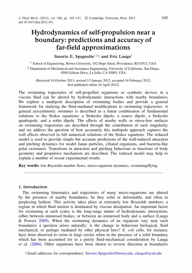
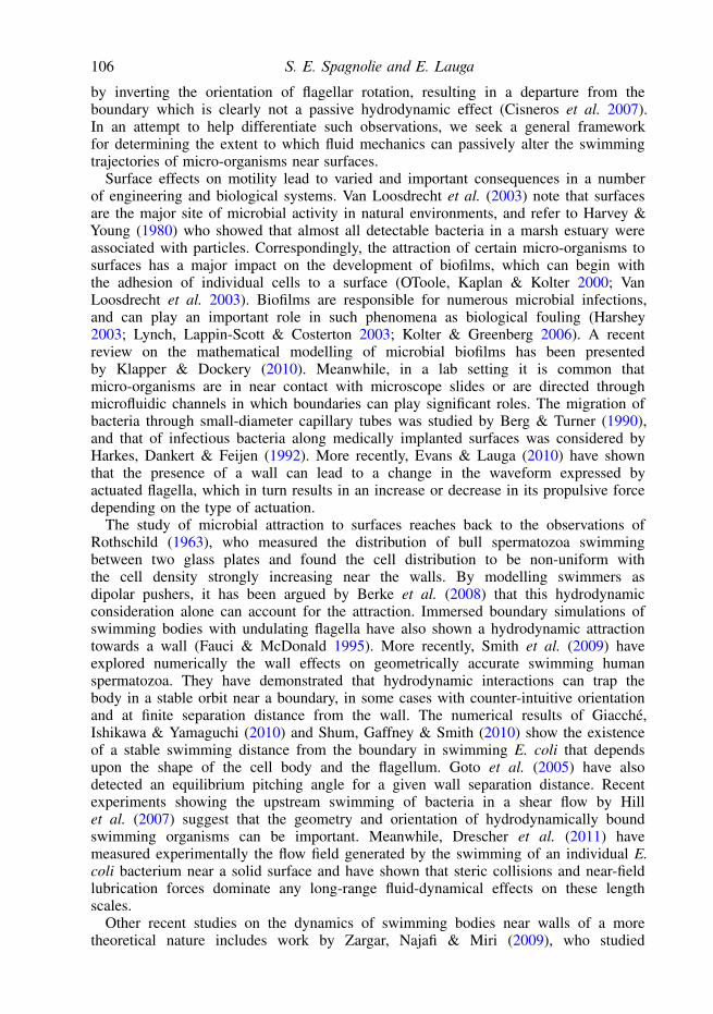
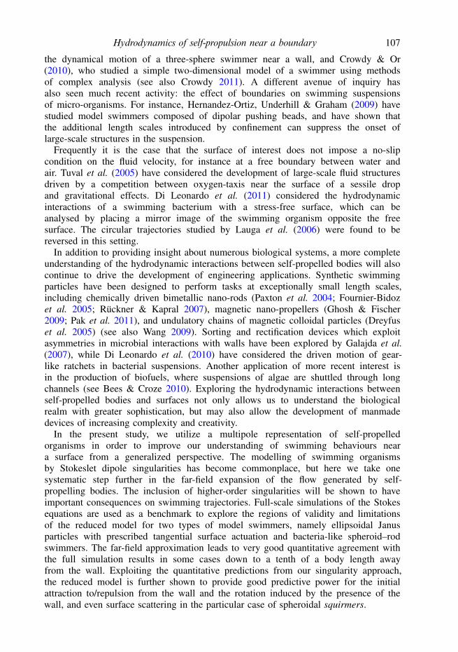
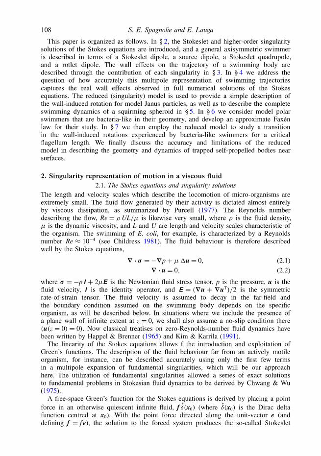
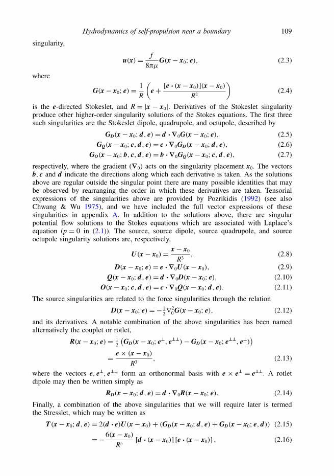
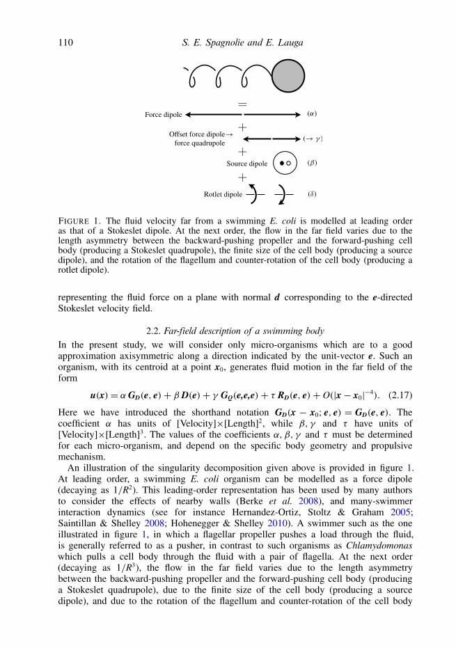

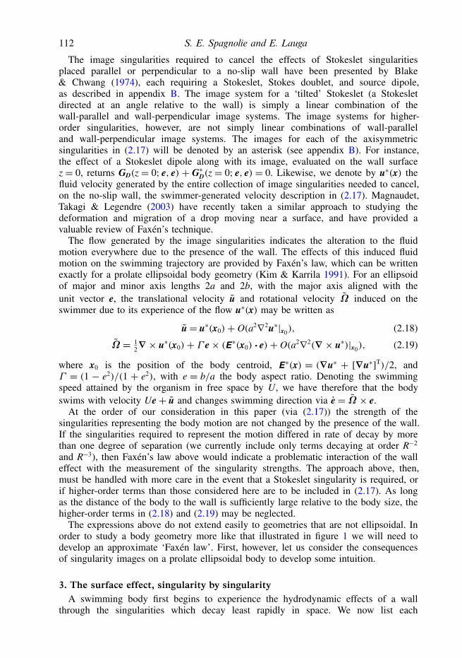

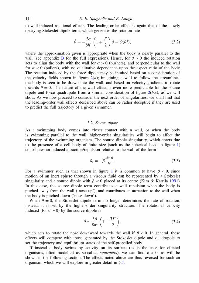

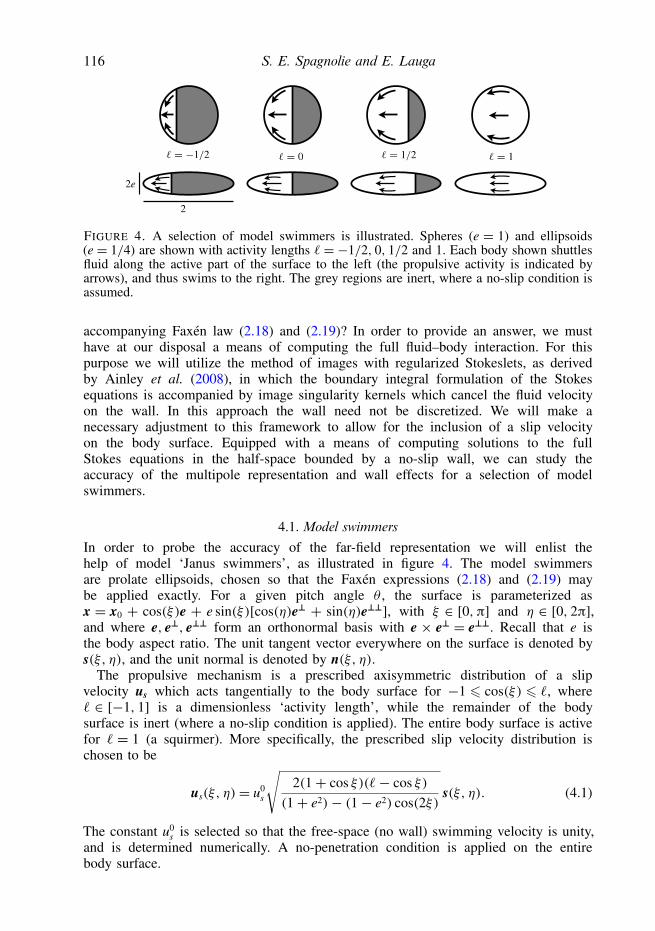
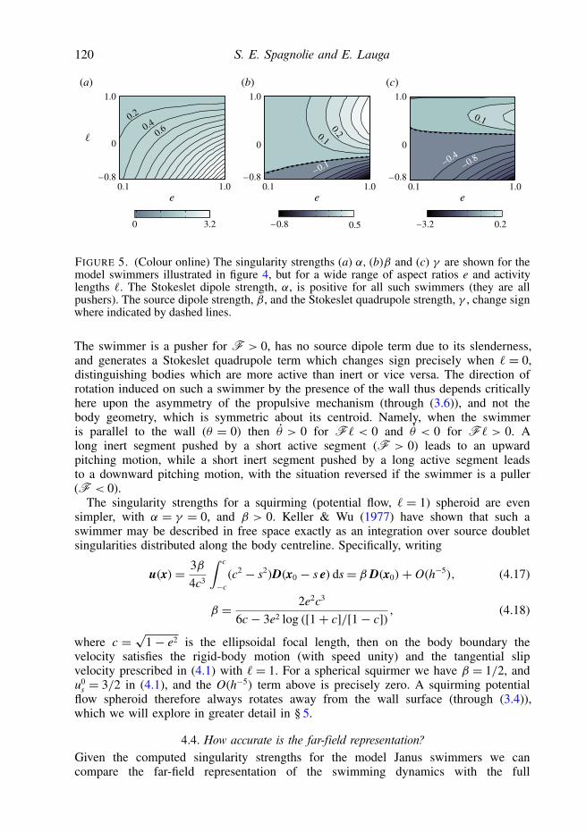
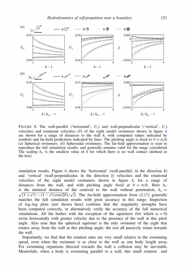
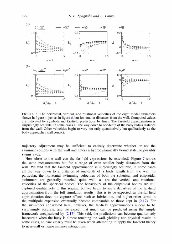
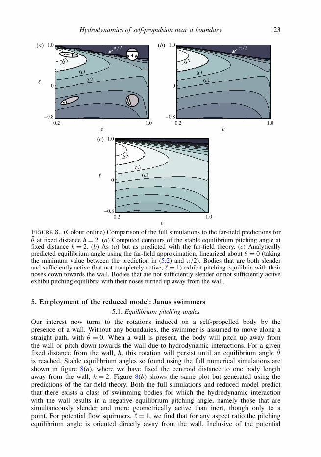
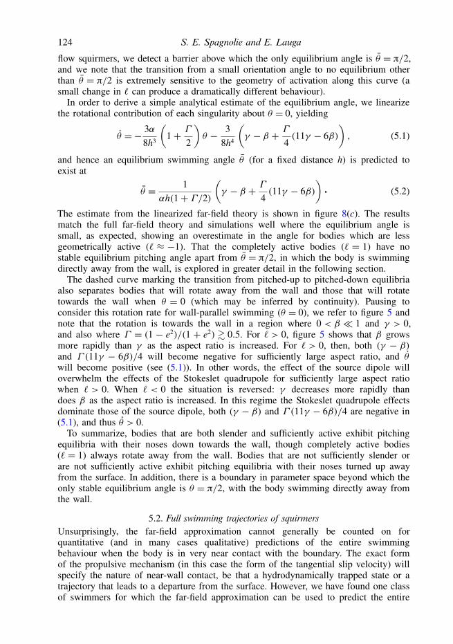

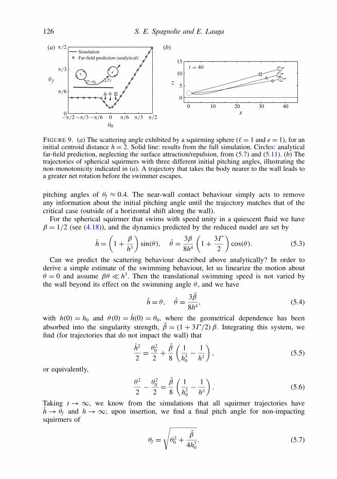


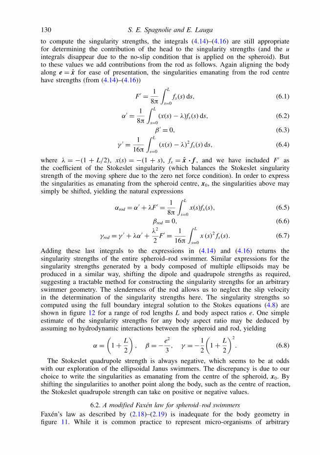
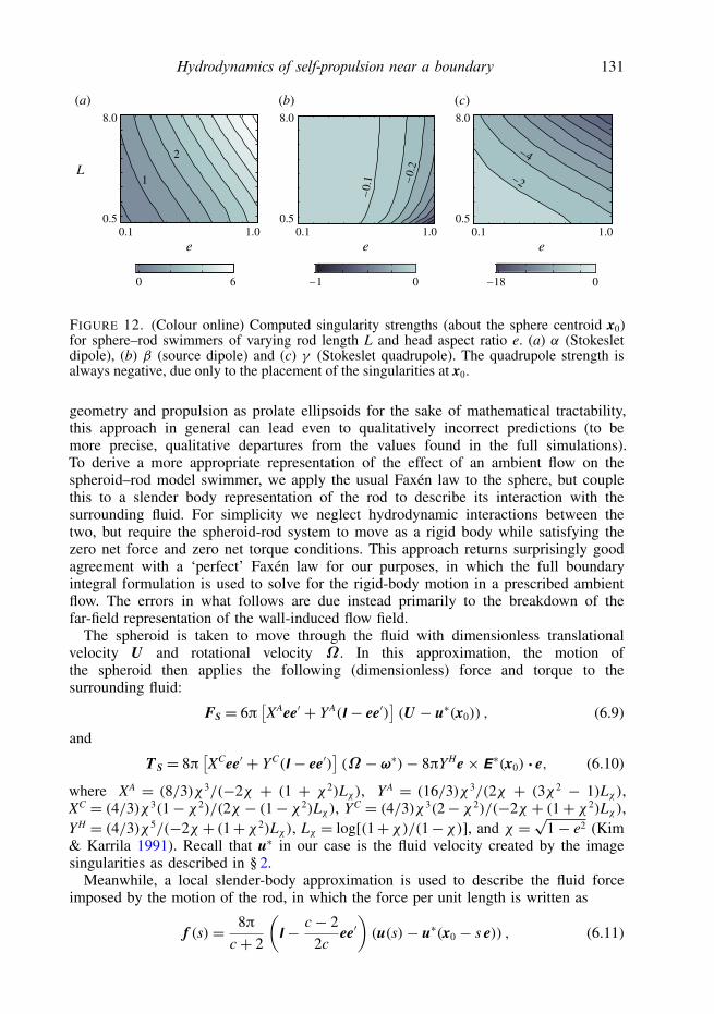
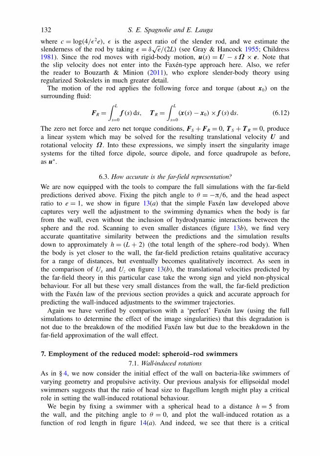
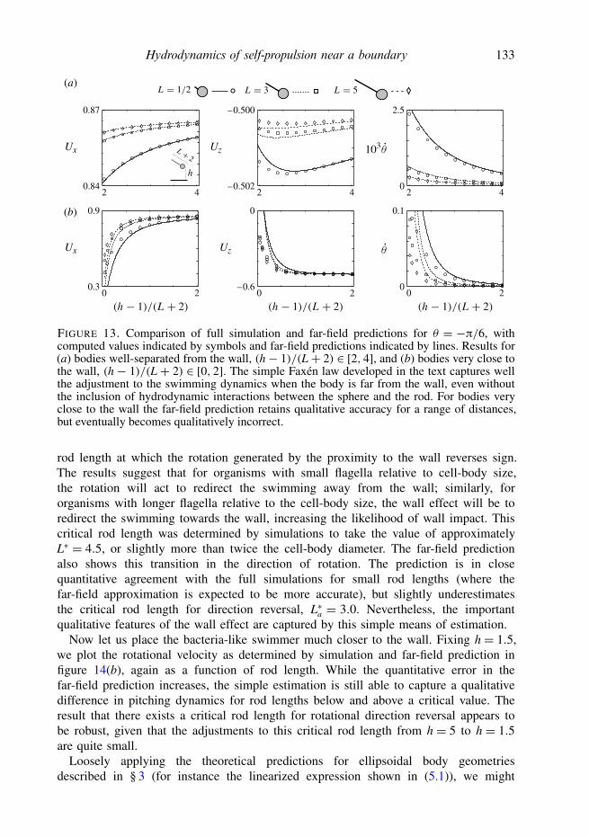
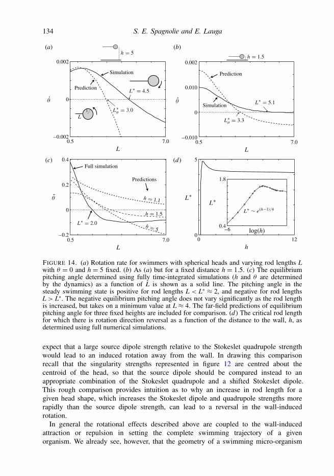
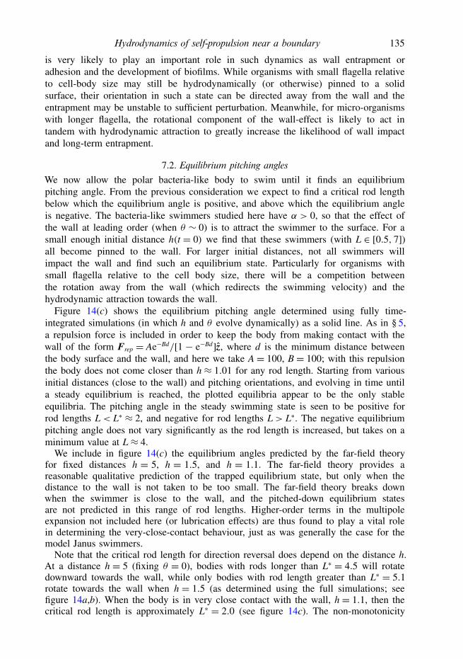
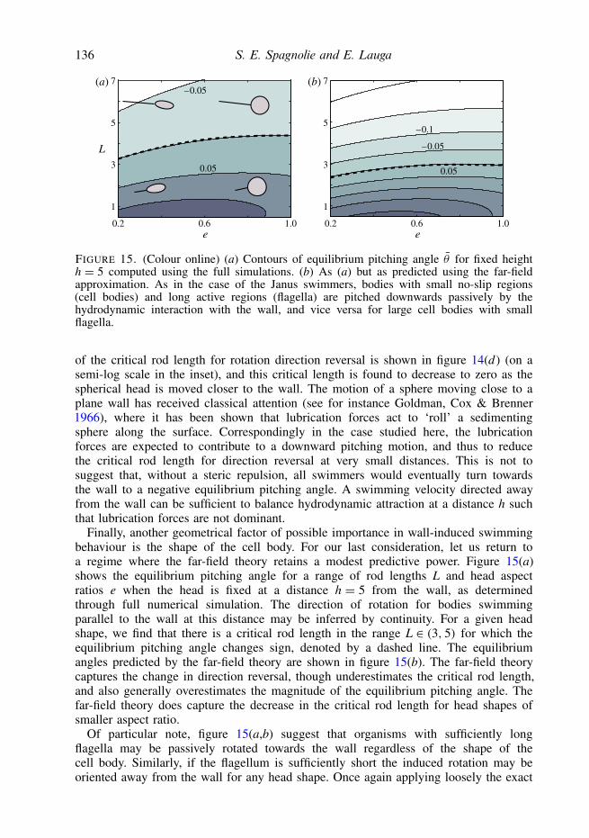

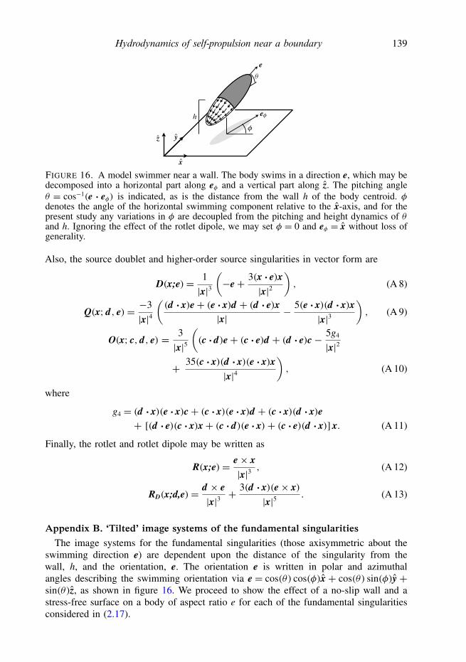

![arXiv:1208.0880v1 [cond-mat.stat-mech] 4 Aug 2012](https://static.documents.pub/doc/80x56/61c91749592343042f1a5657/arxiv12080880v1-cond-matstat-mech-4-aug-2012.jpg)


