J. Fluid Mech. (2017), vol. 830, pp. 439–478. c Cambridge University Press 2017 doi:10.1017/jfm.2017.513 439 Unsteady aerodynamics and vortex-sheet formation of a two-dimensional airfoil X. Xia 1 and K. Mohseni 1, 2, † 1 Department of Mechanical and Aerospace Engineering, University of Florida, Gainesville, FL 32611-6250, USA 2 Department of Electrical and Computer Engineering, University of Florida, Gainesville, FL 32611-6250, USA (Received 17 October 2016; revised 24 May 2017; accepted 25 July 2017; first published online 2 October 2017) Unsteady inviscid flow models of wings and airfoils have been developed to study the aerodynamics of natural and man-made flyers. Vortex methods have been extensively applied to reduce the dimensionality of these aerodynamic models, based on the proper estimation of the strength and distribution of the vortices in the wake. In such modelling approaches, one of the most fundamental questions is how the vortex sheets are generated and released from sharp edges. To determine the formation of the trailing-edge vortex sheet, the classical steady Kutta condition can be extended to unsteady situations by realizing that a flow cannot turn abruptly around a sharp edge. This condition can be readily applied to a flat plate or an airfoil with cusped trailing edge since the direction of the forming vortex sheet is known to be tangential to the trailing edge. However, for a finite-angle trailing edge, or in the case of flow separation away from a sharp corner, the direction of the forming vortex sheet is ambiguous. To remove any ad hoc implementation, the unsteady Kutta condition, the conservation of circulation as well as the conservation laws of mass and momentum are coupled to analytically solve for the angle, strength and relative velocity of the trailing-edge vortex sheet. The two-dimensional aerodynamic model together with the proposed vortex-sheet formation condition is verified by comparing flow structures and force calculations with experimental results for several airfoil motions in steady and unsteady background flows. Key words: aerodynamics, swimming/flying, vortex shedding 1. Introduction Mankind has been dreaming to fly for centuries. However, the fundamental flying mechanism had not been understood until the pioneers of aerodynamics, such as Kutta and Joukowski (Milne-Thomson 1958), connected lift generation to the circulation of an airfoil in the steady sense. Over the last several decades, in order to design high-performance micro aerial vehicles (MAVs), major research effort has been focused on unveiling the unsteady aerodynamic secrets of insects and birds that have † Email address for correspondence: mohseni@ufl.edu Downloaded from https://www.cambridge.org/core . University of Florida , on 26 Oct 2017 at 17:18:59, subject to the Cambridge Core terms of use, available at https://www.cambridge.org/core/terms . https://doi.org/10.1017/jfm.2017.513
Unsteady aerodynamics and vortex-sheetformation of a two-dimensional airfoil
X. Xia1 and K. Mohseni1,2,†1Department of Mechanical and Aerospace Engineering, University of Florida,
Gainesville, FL 32611-6250, USA2Department of Electrical and Computer Engineering, University of Florida,
Gainesville, FL 32611-6250, USA
(Received 17 October 2016; revised 24 May 2017; accepted 25 July 2017;first published online 2 October 2017)
Unsteady inviscid flow models of wings and airfoils have been developed to study theaerodynamics of natural and man-made flyers. Vortex methods have been extensivelyapplied to reduce the dimensionality of these aerodynamic models, based on theproper estimation of the strength and distribution of the vortices in the wake. Insuch modelling approaches, one of the most fundamental questions is how the vortexsheets are generated and released from sharp edges. To determine the formation ofthe trailing-edge vortex sheet, the classical steady Kutta condition can be extendedto unsteady situations by realizing that a flow cannot turn abruptly around a sharpedge. This condition can be readily applied to a flat plate or an airfoil with cuspedtrailing edge since the direction of the forming vortex sheet is known to be tangentialto the trailing edge. However, for a finite-angle trailing edge, or in the case of flowseparation away from a sharp corner, the direction of the forming vortex sheet isambiguous. To remove any ad hoc implementation, the unsteady Kutta condition, theconservation of circulation as well as the conservation laws of mass and momentumare coupled to analytically solve for the angle, strength and relative velocity of thetrailing-edge vortex sheet. The two-dimensional aerodynamic model together with theproposed vortex-sheet formation condition is verified by comparing flow structuresand force calculations with experimental results for several airfoil motions in steadyand unsteady background flows.
Mankind has been dreaming to fly for centuries. However, the fundamental flyingmechanism had not been understood until the pioneers of aerodynamics, such as Kuttaand Joukowski (Milne-Thomson 1958), connected lift generation to the circulationof an airfoil in the steady sense. Over the last several decades, in order to designhigh-performance micro aerial vehicles (MAVs), major research effort has beenfocused on unveiling the unsteady aerodynamic secrets of insects and birds that have
demonstrated unrivalled manoeuverability and agility. Early researchers (Ellington1984; Dickinson & Gotz 1993) have attributed the high lift performance of the naturalflyers to an attached leading-edge vortex (LEV). Later, numerous investigations (Liu& Kawachi 1998; Dickinson, Lehmann & Sane 1999; Sun & Tang 2002; Wang,Birch & Dickinson 2004; Lua, Lim & Yeo 2008; Kim & Gharib 2010; DeVoria &Ringuette 2012; Cheng et al. 2013; Liu et al. 2015a; Polet, Rival & Weymouth 2015;Onoue & Breuer 2016; Xu & Wei 2016) have been carried out to study the dynamicsof the wake vortices as well as its effects on force generation for wings or airfoilsundergoing unsteady motions, such as accelerating, pitching, flapping, etc.
For theoretical investigation, inviscid potential flow together with vortex methodshave been extensively applied to provide a reduced flow model without solving theNavier–Stokes equation. For example, Minotti (2002) adopted a virtual coordinateframe to develop an unsteady framework for a two-dimensional (2-D) rotating flatplate and employed a single point vortex to emulate the effect of the LEV. However,the single vortex was still modelled in a quasi-steady manner that the location andcirculation of the vortex are fixed during the movement of the plate. Michelin &Smith (2009), Wang & Eldredge (2013) and Hemati, Eldredge & Speyer (2014)modelled the wake using finite sets of point vortices with varying strengths andevolving locations. This resulted in significant improvement in capturing the unsteadyfeatures of the flow; whereas the accuracy of the model is still limited, especiallyfor cases with complex near-field wake patterns, due to the overly reduced modellingof the vortical structures. An alternative approach is to fully represent the wakevortex sheets in a discretized sense, using either point vortices or vortex panelsas demonstrated by Katz (1981), Streitlien & Triantafyllou (1995), Jones (2003),Yu, Tong & Ma (2003), Pullin & Wang (2004), Ansari, Zbikowski & Knowles(2006a,b), Shukla & Eldredge (2007), Xia & Mohseni (2013a), Ramesh et al. (2014)and Li & Wu (2015). Due to a relatively complete representation of all vorticalstructures in the wake, the vortex-sheet approach generally yields promising accuracy;however, the simulation becomes increasingly expensive as time proceeds. As aremedy, a vortex-amalgamation method (Xia & Mohseni 2013b, 2015) has recentlybeen proposed to effectively restrain the growth of the computational cost for largesimulations.
In practice, our previous model (Xia & Mohseni 2013a) for a 2-D unsteady flatplate could be readily applied to the case of a rigid wing or airfoil with negligiblethickness. However, the same extension might not be applicable for an airfoil asthe model requires us to establish an analytical mapping between the airfoil and acircle. Although special solutions for certain types of airfoil could exist (such asthe Joukowski airfoil), it is generally challenging to obtain such transformation foran arbitrary-shaped airfoil. To address this difficulty, the effect of the airfoil mightbe substituted by a closed vortex sheet coinciding with the surface of the airfoil,the framework of which is consistent with the boundary-element method (Morino &Kuo 1974; Katz 1981; Katz & Plotkin 1991; Zhu et al. 2002; Jones 2003; Shukla &Eldredge 2007; Pan et al. 2012).
The essence of vortex-based flow models lies in the accurate predictions of thestrength and distribution of the vortices in the flow field. Since the evolution of freevortices follows the Birkhoff–Rott equation (Lin 1941; Rott 1956; Birkhoff 1962),the key problem to be addressed is how vorticity detaches from the surface of thesolid body and enters the flow. In reality, the generation of vorticity is related tothe fluid–solid interaction that forms the shear layer, which is essentially the productof the viscous effect. Under the framework of inviscid flow, a typical solution is
to apply vorticity releasing conditions at the vortex shedding locations of the solidbody, e.g. the Kutta condition at a sharp trailing edge. This means that all theviscous effects can be translated into a single condition (Crighton 1985) that yieldsan estimation of the circulation around the body or the vorticity created near eachvortex shedding location. For trailing edges, the classical Kutta condition has beenshown to be effective for steady background flows, thus it is also commonly knownas the steady-state trailing-edge Kutta condition which requires a finite velocity at thetrailing edge (Saffman & Sheffield 1977; Huang & Chow 1982; Mourtos & Brooks1996). For a Joukowski airfoil, the steady-state Kutta condition is realized by settingthe trailing edge to be a stagnation point in the mapped circle plane. The effect ofthis implementation is that the stagnation streamline from the trailing edge will betangential to the edge (or bisect a finite-angle trailing edge), which is consistent withthe physical flow near the trailing edge. For the case of a flat plate, this condition willguarantee the streamline emanating from this stagnation point to be in line with theplate, fulfilling the condition proposed in previous studies (Chen & Ho 1987; Poling& Telionis 1987). However, the stagnation streamline for a finite-angle trailing edgeis ambiguous (Poling & Telionis 1986), which a causes great challenge to modellingthe trailing-edge vortex (TEV) sheet.
To address this difficulty, an additional relationship other than the Kutta conditionis necessary. Realizing that the flow field is obtained by solving the Euler equation,which is the Navier–Stokes equation without the viscous term, this flow modelgenerally has difficulty in capturing viscous effects around and behind a movingobject. The introduction of the vortex sheet could partially address this difficulty.Physically, a vortex sheet represents a viscous shear layer in the Euler limit, byletting the thickness of the shear layer approach zero (Saffman 1992, §2.2). From akinematic perspective, this approximation would yield the solution to the inviscid flowoutside the vortex sheet with the non-penetration boundary condition implemented atthe fluid–solid interface. However, a vortex sheet is inadequate to represent a viscousshear layer in the dynamic sense. This is because the vortex sheet only conserves thetangential velocity jump, which is also the circulation per unit length of the originalshear layer. Therefore, a vortex sheet does not resolve the velocity gradient across thesheet; neither does it account for the mass and momentum associated with the shearlayer, nor the fluid entrained by the shear layer. To this end, a vortex-sheet-based flowmodel is likely to capture the force contributions from circulation, i.e. lift and pressuredrag, but not the viscous drag which is closely related to the momentum balance ofthe viscous shear layer. In order to properly capture other viscous effects, such asentrainment, viscous drag or even energy dissipation, we propose a generalized sheetwith superimposed quantities and discontinuities associated with the original shearlayer. This enables the application of the conservation laws of mass and momentumfor a flow system containing a vortex sheet. As seen in this paper, application ofproper boundary conditions together with standard conservation laws allow for thecalculation of a correct wall-bounded vortex sheet as well as the free vortex sheetreleased at the trailing edge of an airfoil.
The paper is outlined as follows. The framework of the vortex-sheet-basedaerodynamic model is presented in § 2. Section 3 provides an implicit expressionof the unsteady Kutta condition, which relates the strength of the forming vortexsheet to its adjacent bound vortex sheet. Section 4 introduces a generalized sheetmodel, which is applied to the particular case of the finite-angle trailing edge toderive a momentum balance relation. Then, the momentum balance relation and theconservation of circulation are incorporated in § 5 to obtain an explicit form of the
FIGURE 1. (Colour online) Diagram showing the unsteady flow model of an airfoil.
unsteady Kutta condition, which allows analytical calculation of the angle, strengthand shedding velocity of the trailing-edge vortex sheet. The numerical implementationand validations of this aerodynamic model are presented in § 6.
2. Unsteady aerodynamic modelThe framework of the aerodynamic model for a 2-D airfoil is not fundamentally
different from that for a 2-D flat plate (Xia & Mohseni 2013a). In both situations,potential flow is applied as the governing equation, which is based on solving theNavier–Stokes equation in the Eulerian limit. This has two main advantages: one isanalytical representation of the entire flow field, the other is saving computational costsince the domain of interest is reduced from the entire flow field to only finite vorticalstructures.
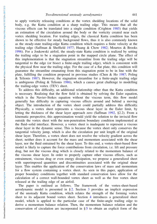
2.1. Vortex-sheet-based flow modelAssume that the rigid-body motion of the airfoil in a quiescent environment can bedecomposed into a translational motion of velocity −U(t) and a rotational motionof angular velocity Ω(t). Both the translational and the rotational motions can beincorporated into the boundary condition at the solid–fluid interface. As shown infigure 1, flow separation near the leading edge and at the sharp trailing edge of theairfoil causes the formation of two free vortex sheets in the wake. In a Cartesiancoordinate system with the origin fixed at the rotation centre, the complex potentialof the flow around an airfoil with angle of attack, α(t), can be formulated as
w(z, t) = −i
2π
[ ∫ SL(t)
0ln(z− zL(s, t))γL(s, t) ds︸ ︷︷ ︸
LEV term
+
∫ ST (t)
0ln(z− zT(s, t))γT(s, t) ds︸ ︷︷ ︸
TEV term
]+wb(z, t)︸ ︷︷ ︸
Body term
, (2.1)
where z is the complex position, s is the curve length between the separation point anda vortex element along a vortex sheet and γ is the vortex-sheet strength (circulation
per unit length). The subscripts L and T denote the properties associated with theleading-edge and trailing-edge vortex sheets, respectively. So SL and ST represent thetotal lengths of the leading-edge and trailing-edge vortex sheets, respectively.
In (2.1), wb(z, t) represents the flow induced by the body motion of the airfoil,and is usually associated with the so-called ‘bound vortex’. Therefore, the ‘boundvortex’ can be viewed as a substitute for the solid body so that the non-penetrationboundary condition can still be satisfied at the fluid–solid interface while the solidbody is removed from the flow model. Again, we note here that the ‘body term’or the ‘bound vortex’ implicitly accounts for the effects of translation, rotation ordeformation, and more details will be provided in § 2.2. In general, the ‘bound vortex’can be realized by placing image vortices inside the solid body for a Joukowski airfoilor a flat plate, where the strength and location of the image vortices can be firstdecided from Milne-Thomson’s circle theorem (Milne-Thomson 1958) in the circleplane and then mapped back to the physical plane. However, for an arbitrarily shapedairfoil which cannot be easily mapped to a circle, an analytical solution for wb(z, t)is not available. In this case, the ‘bound vortex’ can be realized by placing a boundvortex sheet along the surface of the airfoil as shown in figure 1, and wb(z, t) becomes
wb(z, t)=−i
2π
∫ SB(t)
0ln(z− zB(s, t))γB(s, t) ds, (2.2)
where the subscript B denotes the properties associated with the bound vortex sheet.Note here that s for the bound vortex sheet starts from the trailing edge with a counter-clockwise direction, and SB is the total length of the bound vortex sheet.
Combining (2.1) and (2.2) and taking the derivative dw/dz, we obtain the complex-conjugate velocity field, V(z, t)= u(z, t)− iv(z, t), in the form
V(z, t) = −i
2π
[ ∫ SL(t)
0
γL(s, t) dsz− zL(s, t)︸ ︷︷ ︸
LEV term
+
∫ ST (t)
0
γT(s, t) dsz− zT(s, t)︸ ︷︷ ︸
TEV term
+
∫ SB(t)
0
γB(s, t) dsz− zB(s, t)︸ ︷︷ ︸
Bound vortex sheet term
]. (2.3)
It should be noted that the velocity field represented by (2.3) is singular on the vortexsheets, where the jump of the tangential component of velocity is equal to the strengthof the vortex sheet (Saffman 1992). More details regarding the evaluation of the vortexsheets will be discussed in §§2.2 and 3. At this point, the calculation of the entire flowfield is reduced to determining the strength and distribution of only a few finite lengthvortex sheets.
2.2. Bound vortex sheetThe instantaneous velocity field around an airfoil can now be decided if the twofree vortex sheets and one bound vortex sheet are given. This requires knowing thestrengths and positions of the vortex sheets (γL, γT, γB, zL, zT, zB). Considering thecase where the flow initially remains fully attached, this indicates no flow separationor free vortex sheet existed at t = 0. Under this assumption, γL, γT , zL, zT for latertimes might be found through solving the formation and evolution of the free vortexsheets. So we assume that γL, γT , zL, zT are known in order to solve the bound vortex
sheet at any given time. Furthermore, the position of the bound vortex sheet, zB, isalso known as it coincides with the surface of the airfoil at any time. As a result,the main task here is to solve for the vortex-sheet strength γB. We should note that abound vortex sheet is treated differently from a free vortex sheet since zB is prescribed.Actually, the free vortex sheet is applied to represent the physical free shear layer,while the bound vortex sheet is introduced to ‘mimic’ the effect of a solid boundary.Therefore, it is expected that the primary role of the bound vortex sheet is to satisfythe non-penetration boundary condition, which can be expressed as
u(z′) · n(z′)= ub(z′) · n(z′) for z′ = zB(s′) and 0 6 s′ 6 SB, (2.4)
where u(z′) = (u(z′), v(z′)) is the flow velocity at the surface of the airfoil, zB, andn(z′) is the unit normal vector to the surface. Note that the definitions for z′ ands′ only apply to the current section. Also, time t is dropped here and in followingderivations for simplicity although they should be satisfied instantaneously. ub(z′) isthe velocity associated with the surface element of the airfoil so it generally describesthe deformation of an airfoil. However, ub(z′) can be also applied to account forthe translational motion in the complex-conjugate form, −|U|e−iα, and the rotationalmotion in the complex-conjugate form, −iΩ z′, where z′ denotes the complex conjugateof z′.
Since the bound vortex sheet is placed at the surface of the airfoil, it creates avelocity jump across zB. Based on (2.3) and the definition of a vortex sheet (Saffman1992), the two limiting values for u±(z′)− iv±(z′)= V±B (z′) can be derived as
V±B (z′) = −
i2π
[∫ SL
0
γL(s) dsz′ − zL(s)
+
∫ ST
0
γT(s) dsz′ − zT(s)
+−
∫ SB
0
γB(s) dsz′ − zB(s)
]±
12γB(s′)
dz′
|dz′|, (2.5)
where −∫
denotes the Cauchy principal value which excludes the vorticity at z′ fromthe integral. dz′|dz′|−1 is the complex form of the unit tangential vector, s(z′), atthe surface of the airfoil. With s(z′) pointing in the counter-clockwise direction ofthe airfoil body, V+B (z′) becomes the velocity limit when the bound vortex sheetis approached from the outside of the airfoil, whereas V−B (z′) is the velocity limitwhen the vortex sheet is approached from the inside. Since u(z′) is the flow velocityoutside the surface of the airfoil, it should take the value V+B (z′). With n(z′) writtenas −i dz′|dz′|−1, equation (2.4) has the complex form
Re[
V+B (z′)+ |U|e−iα
+ iΩ z′] −i dz′
|dz′|
= 0. (2.6)
Ideally, equation (2.6) would give the strength of the bound vortex sheet, γB, if γL,γT , zL, zT and zB are given. However, a general analytical solution to (2.6) does notexist for an arbitrarily shaped airfoil. Fortunately, it is possible to solve this problemnumerically by discretizing the bound vortex sheet into piecewise linear vortex panels,the details of which will be discussed in § 6.1.
It should be noted that the strength of the bound vortex sheet γB can be expressed asγB= uf · s, where uf represents the potential flow velocity at the fluid–solid boundary.With a no-slip boundary condition, γB can be divided into two terms, γb and γγ ,according to Eldredge (2010). γb is purely associated with the body-surface motion
relative to the reference frame, and it can be estimated from γb = ub · s. γγ is thephysical vortex sheet corresponding to the viscous shear layer, which is given byγγ = γB− γb. Therefore, γγ is invariant regardless of the reference frame being globalor body fixed, while both γb and γB could change as the reference frame changes. Toavoid ambiguity, γB in this study only represents the bound vortex sheet in the globalreference frame.
2.3. Force and torqueFollowing previous studies (Wu 1981; Eldredge 2010), the aerodynamic force appliedon the airfoil can be estimated based on the rate of change of the total impulse inthe form
F=−ρddt
∫∑
Sx× γ ds, (2.7)
where x is the position vector of a vortex-sheet element. γ = γ k, where k is the unitvector normal to the 2-D plane and γ in this work should be substituted with γL, γT
and γB for SL, ST and SB, respectively. ρ is the density.∑
S represents the entirevortex-sheet system,
∑S = SL + ST + SB. Similarly, the total torque exerted by the
fluid on the airfoil can be obtained from
Tτ =−ρd
2 dt
∫∑
Sx× (x× γ ds). (2.8)
The main advantage of (2.7) and (2.8) is that the calculations of force and torque arecompletely transformed into the dynamics of the bound and wake vortices, which canbe explicitly obtained from this aerodynamic model. Equations (2.7) and (2.8) will beused to estimate aerodynamic force and torque for all simulations in § 6.
3. Unsteady Kutta condition
To implement the above-proposed flow model, we need to determine the intensitiesand locations of the wake vortices, i.e. γL, γT , zL and zT associated with the leading-edge and trailing-edge vortex sheets at any given time. Assuming no wake vortexinitially, the task requires understanding the formation and evolution of the leading-edge and trailing-edge vortex sheets. To this end, the evolution of a free vortex sheetis dictated by the Helmholtz laws of vortex motion (Helmholtz 1867; Saffman 1992).According to the third Helmholtz law, the circulation of a vortex-sheet element can betreated as time invariant once it is detached from the airfoil. Furthermore, the secondHelmholtz law dictates that a vortex element and its overlapping fluid particle shouldmove together. In accordance with these principles, the velocity describing the motionof an element on a free vortex sheet can be derived using the Birkhoff–Rott equation(Lin 1941; Rott 1956; Birkhoff 1962), the formulation of which is similar to (2.3),with
∫replaced by −
∫to remove the self-induced singularity of a vortex element. This
gives the basic principle for evolving vortices in the wake. The only question left ishow vorticity is generated and detached from the surface of the airfoil to form wakevortex sheets. We note that in reality vortex sheets could come off the airfoil frommultiple separation points. However, the current study only focuses on vortex sheddingat a sharp trailing edge, which is the most common vortex generation mechanism.
3.1. Previous studies and main challengeWe first consider a simple case, where the vortex sheet is formed at the edge of a flatplate or a cusped trailing edge of an airfoil. Without considering the viscous effect, atypical way of deciding the vortex-sheet formation at the trailing edge is the classicalsteady Kutta condition. This condition requires the flow velocity at the trailing edge tobe finite or the loading at the trailing edge to be zero, based on the physical sense thatflow cannot turn around a sharp edge. The application of this condition for a flat plateor a Joukowski airfoil (with cusped trailing edge) has already been demonstrated inseveral previous works (Streitlien & Triantafyllou 1995; Yu et al. 2003; Ansari et al.2006a; Xia & Mohseni 2013a) among others. Basically, this condition is equivalentto enforcing a stagnation point at the trailing edge in the transformed circle plane.However, Xia & Mohseni (2014) recently pointed out that a stagnation point generallydoes not exist at the trailing edge for the case of body rotation. As a result, theyproposed to implement the unsteady Kutta condition by relaxing the trailing-edge pointof the circle plane from totally stagnant to only stagnant in the tangential directionof the surface, which still conforms to the classical Kutta condition in the sense ofpreventing flow around the sharp edge. Here, we emphasize that these steady andunsteady Kutta conditions are problem dependent, meaning they only apply to a flatplate or an airfoil that can be mathematically mapped to a circle.
Alternatively, Jones (2003) modelled the flow around a flat plate using a boundvortex sheet coincident with the plate and two free vortex sheets that are emanatingfrom the plate’s two sharp edges, which is similar to the flow model presented herefor an airfoil. By removing the singularities of the flow velocity at the trailing edge,which complies with the classical Kutta condition that flow velocity should be finiteat a sharp edge, Jones managed to derive an analytical unsteady Kutta condition. Thiscondition can be summarized as follows:
(i) γg = γE;(ii) ug = uE;
(iii) θg = 0.
Here, γg, ug and θg represent the strength, tangential velocity (relative to the edge),and angle (relative to the tangent of the plate) of the forming vortex sheet, respectively.γE is the strength of the bound vortex sheet at the sharp edge, and uE is the averagetangential slip between the bound vortex sheet and the plate at the edge. Therefore,Jones’ unsteady Kutta condition allows the analytical calculation of the strength,velocity and direction of the forming vortex sheet for the sharp edge of a flat plateor a cusped airfoil, based on the existing bound vortex sheet. However, the currentwork is concerned with a general-shaped airfoil, for which Jones’ unsteady Kuttacondition might not be suitable. Specifically, if there is a finite angle, 1θ0 ∈ [0, π),between the upper and lower surfaces of the trailing edge, θg, of the forming vortexsheet would be ambiguous.
This challenge is further explained below. Since the forming vortex sheet moveswith the fluid as a material sheet, it resembles a streakline released from the trailingedge in the body-fixed reference frame. Recognizing that at the origin of a streaklinethe directions of the streakline and the streamline are identical to each other, thisindicates that the ambiguity of the vortex-sheet direction is equivalent to the ambiguityof the stagnation streamline direction. In fact, for steady trailing-edge flow where theshedding of vorticity vanishes (γg= 0), Poling & Telionis (1986) pointed out that thesteady Kutta condition requires the stagnation streamline to bisect the wedge angleof a finite-angle trailing edge. Otherwise, an unbalance between the upper and lower
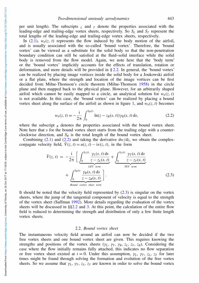
FIGURE 2. (Colour online) The vortex-sheet configuration for (3.2).
shear layers near the trailing edge would cause a non-zero vorticity generation whichwould be naturally unsteady. According to this argument, an unsteady trailing-edgeflow naturally generates vorticity and causes the stagnation streamline to divert fromthe wedge bisector line, which has been confirmed experimentally (Ho & Chen 1981;Poling & Telionis 1986). A prominent theory for the unsteady situation has beenproposed by Giesing (1969) and Maskell (1971) that the stagnation streamline is anextension of one of the two tangents at the trailing edge. Although Basu & Hancock(1978) has provided extensive discussion supporting the Giesing–Maskell model, anotable drawback of this model is that it does not reduce to the steady-state solutionin the limit of vanishing vorticity. Furthermore, Poling & Telionis (1986) reportedthat the Giesing–Maskell model holds approximately for large rate of vorticitygeneration, whereas the stagnation streamline direction changes smoothly between thetwo tangents of the trailing edge when vorticity generation is low.
3.2. The condition for a finite-angle trailing edgeIn this study, we seek to derive an unsteady Kutta condition for a finite-angle trailingedge to analytically determine γg, ug, and θg associated with the forming vortex sheet.According to our previous study of an unsteady flat plate (Xia & Mohseni 2013a,2014), the unsteady Kutta condition can be implemented numerically by satisfying thecondition
ug · ng = 0, (3.1)
where ug is the vector form of the vortex-sheet velocity relative to the trailing edgeand ng is the unit vector normal to the vortex sheet at the trailing edge as shownin figure 2. Basically, equation (3.1) enforces the streamline to be tangential to theforming vortex sheet.
Here, we shall extend (3.1) to the situation of a finite-angle trailing edge to expressug in terms of γg and θg, as well as other parameters associated with the instantaneousbackground flow and the bound vortex sheet. We assume the flow field changessmoothly so that all vortex sheets are smooth curves near the trailing edge andtheir strengths also vary smoothly along the sheets. The vortex-sheet system for thiscalculation is illustrated in figure 2, where γ1 and γ2 are the bound vortex strengthsand γg is the strength of the forming vortex sheet as it approaches the trailing edge.Noting that the vortex-sheet strength is not well defined at the trailing-edge point,
where γ1, γ2 and γg are discontinuous with each other, the trailing-edge point isactually a singularity point in the vortex-sheet system. Fortunately, according to theBirkhoff–Rott equation (Lin 1941; Rott 1956; Birkhoff 1962), ug should be estimatedin the desingularized flow field excluding the vorticity at the trailing edge point. Thisallows us to represent ug, based on the vortex-sheet configuration of figure 2 and(2.3), in the limit form
Vg = −i
2πlimε→0
[∫ SL
0
γL(s) dszT(0)− zL(s)
+
∫ ST
ε
γT(s) dszT(0)− zT(s)
+
∫ SB1
ε
γγ 1(s) dszT(0)− zB1(s)
+
∫ SB2
ε
γγ 2(s) dszT(0)− zB2(s)
]+ VCT, (3.2)
where VCT is the velocity difference associated with the coordinate transformationfrom the global reference frame to the body-fixed reference frame. t in (2.3) isdropped here for brevity. Recall the discussion of the bound vortex sheet in § 2.2,γγ (s) rather than γB(s) should be used here for velocity calculation because γb(s)= 0in the body-fixed reference frame. For convenience, we further divide γγ (s) into twoparts, γγ 1(s) and γγ 2(s), as shown in figure 2. The relationships between the originaland the divided bound vortex sheets are given by γγ 1(s)= γγ (s) and zB1(s)= zB(s) for0< s6SB1, and γγ 2(s)=γγ (SB− s) and zB2(s)= zB(SB− s) for 0< s6 (SB−SB1), whereSB1 and SB2 satisfy SB1+ SB2= SB. In this way, the two bound vortex sheets both ‘stem’from the trailing edge, meaning limε→0 zB1(ε)= limε→0 zB2(ε), and limε→0 γγ 1(ε)= γ1
and limε→0 γγ 2(ε)= γ2.The main challenge of calculating (3.2) is that the integrands of
∫ ST
ε,∫ SB1
εand
∫ SB2
ε
become singular as ε→ 0. As a remedy, we only evaluate its leading-order terms asdemonstrated in appendices A and B. Based on the smoothness assumption of thevortex sheets, there exist finite values, ε1, ε2 and εT , so that γγ 1(s) and zB1(s) aresmooth on [0, ε1], γγ 2(s) and zB2(s) are smooth on [0, ε2], and γT(s) and zT(s) aresmooth on [0, ε2]. Accordingly, equation (3.2) can be divided as
Vg = −i
2πlimε→0
[∫ εT
ε
γT(s) dszT(0)− zT(s)
+
∫ ε1
ε
γγ 1(s) dszT(0)− zB1(s)
+
∫ ε2
ε
γγ 2(s) dszT(0)− zB2(s)
]−
i2π
[∫ SL
0
γL(s) dszT(0)− zL(s)
+
∫ ST
εT
γT(s) dszT(0)− zT(s)
+
∫ SB1
ε1
γγ 1(s) dszT(0)− zB1(s)
+
∫ SB2
ε2
γγ 2(s) dszT(0)− zB2(s)
]+ VCT . (3.3)
Applying appendix A to the first three integrals and appendix B to the last fourintegrals yields
Vg =−i
2πlimε→0
[γge−iθg ln (ε)+ γ1e−iθ1 ln (ε)+ γ2e−iθ2 ln (ε)
]+ Vadd, (3.4)
where Vadd represents all additional terms of o(ln(ε)) as ε → 0. θ1, θ2 and θg
correspond to the angles of the vortex sheets (γγ 1, γγ 2 and γT) in the complexdomain as they approach the trailing edge. Now, we combine (3.4) and ImVgeiθg= 0(the complex form of (3.1)) and then divide both sides by the leading-order term,
ln(ε), to obtain γg + γ1 cos(θg − θ1) + γ2 cos(θg − θ2) = 0. Together with the anglerelations defined in figure 2, the unsteady Kutta condition takes the form
γg = γ1 cos1θ1 + γ2 cos1θ2. (3.5)
For the case of a flat plate or a cusped trailing edge, where both 1θ1 and 1θ2 arezero, equation (3.5) is reduced to γg = γ1 + γ2, which is consistent with condition (i)of § 3.1 given by Jones (2003). For a finite-angle trailing edge, equation (3.5) tells usthat the strength of the forming vortex sheet γg depends on its direction θg and thestrengths of its adjacent bound vortex sheets, γ1 and γ2. In § 5, equation (3.5) will becombined with the momentum balance relation and the conservation of circulation toanalytically determine γg, ug and θg of the forming vortex sheet.
4. Momentum balance at the trailing edgeThe unsteady Kutta condition alone does not give the full information about the
forming vortex sheet at a finite-angle trailing edge. Physically, we believe that theformation of the free vortex sheet is the outcome of the upper and lower shear flowsmerging at the trailing edge. As such, the momentum of the merging process mustbe balanced not only along the direction of the forming vortex sheet but also in thenormal direction. We hypothesize that this momentum balance provides an importantdynamic condition relating to the angle of the forming vortex sheet, in addition to thekinematic condition (i.e. the Kutta condition).
Before we proceed, it is necessary to discuss the main challenges of applyingthe conservation laws of mass and momentum to a system of vortex sheets. Takethe bound vortex sheet as an example, the non-penetration and no-slip boundaryconditions are the physically correct conditions for fluid–solid interactions in mostapplications. While the Navier–Stokes equation allows for the matching of bothnormal and tangential velocity components between the fluid and the solid, the Eulerequation allows only for the matching of the wall-normal velocity component andit does not impose any constraints on the tangential velocity component. In orderto remedy this for large Reynolds number flows, where the Euler equation is oftenaccepted as a suitable model, we superimpose the Euler equations with a physicalvortex sheet, γγ , as introduced in § 2.2 to satisfy the no-slip boundary condition.Therefore, γγ actually represents the physical viscous shear layer at the fluid–solidinterface, in the sense of preserving the tangential velocity jump or the circulationacross the shear layer. As has been demonstrated in § 3.2, the modelling of thephysical vortex sheet allows us to perform calculations related to the formationof a free vortex sheet, especially in term of the sheet strength. However, sincethe thickness and the velocity profile of a viscous shear layer are not resolved bya vortex sheet, the mass and momentum associated with the shear layer are notcaptured. Although this will not directly affect the solution of the original Eulerequation, it would definitely cause unbalanced equations of mass and momentumwithin the vortex sheet, especially in the tangential direction, and thereby affectingthe correct prediction of viscous shear force exerted on the shear layer in inviscidflows.
In this section, a generalized sheet model, which incorporates the mass andmomentum fluxes associated with the original shear layer, is proposed to enablethe correct implementation of the momentum conservation law for a system of vortexsheets. Then, the new sheet model is applied to derive a momentum balance relationfor a control volume of the merging zone near the finite-angle trailing edge.
FIGURE 3. A generalized sheet model to represent a viscous shear layer.
4.1. A generalized sheet model for viscous shear layerIn order to properly model the dynamics of a viscous shear layer, here we proposea generalized sheet model on top of the original vortex sheet where all relevantquantities or discontinuities associated with the viscous shear layer are superimposed.A schematic of this modelling approach is illustrated in figure 3. As a first step, asheet of discontinuity in the streamfunction ψ is placed at the location of the originalvortex sheet, so that Jψ(s)K is equal to the volumetric flow rate of the viscous shearlayer in the form
JψK=∫ δs
0us dn, (4.1)
where δs is the thickness of the shear layer and us is the tangential velocity component.Thus, the mass conservation for the new sheet can be written in the differential form
dρs
dt= ρ
∂JψK∂s− me = 0, (4.2)
where me(s) is the per-unit-length mass entrainment associated with the shear layerand ρs is the per-unit-length density defined as ρs = ρδs.
To apply the momentum conservation law to a shear layer, we define a newdiscontinuity, JχK, in analogy to JψK such that
JχK=∫ δs
0(us)2 dn. (4.3)
Therefore, JχK represents the momentum flux associated with the generalized sheet.Furthermore, it is assumed that the new sheet has a characteristic velocity uI(s) =us
I s, satisfying usI = JχK/JψK. In this way, the momentum flux of the shear layer is
conserved. To further generalize the vortex sheet, we also superimpose a pressurejump, Jp(s)K, a shear stress jump, Jτ(s)K and a surface stress (tension) tensor, T s,which is related to the surface stress ts as ts= s ·T s in two dimensions. Now, applying
the Reynolds transport theorem to a sheet element with a length of 1s, the momentumconservation can be expressed as
ρd(JψKs)
dt= ρ
∂(JψKs)∂t
+ ρ∂(JψKuI)
∂s− meue =−JpKn+ JτKs+∇ · T s, (4.4)
where ue is the velocity of the entrained fluid. We note that by assigning properquantities and discontinuities this new sheet is capable of modelling the dynamics of aviscous shear layer at fluid–fluid or fluid–solid interfaces in single and multiple phaseflows.
Next, we apply (4.2) and (4.4) to a special case, the physical vortex sheet γγaround the surface of an airfoil with free vortex sheets attached. Equation (4.2) canbe integrated around the airfoil to give
ρ∑
JψgK−∫ SB
0me ds= 0, (4.5)
where the∑
term sums up the mass flux drained into each attached free vortex sheet,and JψgK is the streamfunction jump at the origin of a free vortex sheet. Consideringthat fluid is physically entrained from the outer flow into the shear layer, the velocityof the entrained fluid should equal the fluid-side velocity of the bound vortex sheet.This gives ue= uf − ub in the body-fixed reference frame, where ub= us
bs+ unbn. With
the non-penetration boundary condition, we have uf = usf s + un
bn and γγ = usf − us
b.Neglecting surface tension and plugging in (4.2), equation (4.4) can be expanded inthe s and n directions as
ρ
(∂JψK
dt+ JψK
∂usI
∂s+∂JψK∂s
(usI − γγ )
)s= JτKs, (4.6)
0= JpKn. (4.7)
Equation (4.7) is still consistent with previous studies (Saffman 1992; Wu, Ma &Zhou 2006) in that pressure is continuous across a vortex sheet. This means that thegeneralized sheet model does not affect the force balance in the normal direction ofthe sheet. In this sense, equation (2.7) still captures the total force contributed fromthe pressure term. Now, we further integrate equation (4.6) around the airfoil to obtain
Jf τ K= ρ∫ SB
0
(∂JψK
dt+ JψK
∂usI
∂s+∂JψK∂s
(usI − γγ )
)s ds+ ρ
∑JψgKu∗g, (4.8)
where Jf τ K is the jump of the total shear force between the fluid and solid sidesof the vortex sheet around the airfoil. Similar to (4.5), the
∑term sums up the
momentum flux, JχgK, entering each attached free vortex sheet. u∗g is the momentum-based characteristic velocity of a free vortex sheet, satisfying u∗g = JχgK/JψgK. It isnoted that the fluid side of γγ is a free shear surface with zero shear stress, Jf τ K isactually the unsteady viscous drag exerted by the solid body, which is not capturedby (2.7). Similar to that reported by Liu, Zhu & Wu (2015b), the term JψK in thisstudy is also the core parameter in drag generation, while here the calculation isperformed for the unsteady case. Last, we note that other necessary global quantitiesand discontinuities can also be superimposed at the location of the original vortexsheet at the solution level for improved force calculation and accurate prediction ofvortex-sheet formation, as summarized in table 1.
Free vortex sheet γ Free shear surfaces at bothsides
Circulation per unit lengthof wake shear layer
Bound vortex sheet γγ Free shear surface at oneside; no-slip at the otherside
Circulation per unit lengthof body shear layer
Mass-flux sheet JψK Captures the entrainment Mass fluxMomentum-flux sheet JχK Enables the analysis of
momentum transportationMomentum flux
Energy-flux sheet JλK Enables the analysis ofenergy dissipation
Flux of kinetic energy
Stress sheet Jσ K Enables the force analysis,especially the viscous force
Jumps of pressure, shearstress or surface stress
TABLE 1. A summary of the sheet models for a viscous shear layer. JλK is defined asJλK=
∫ δs
0 (us)3 dn.
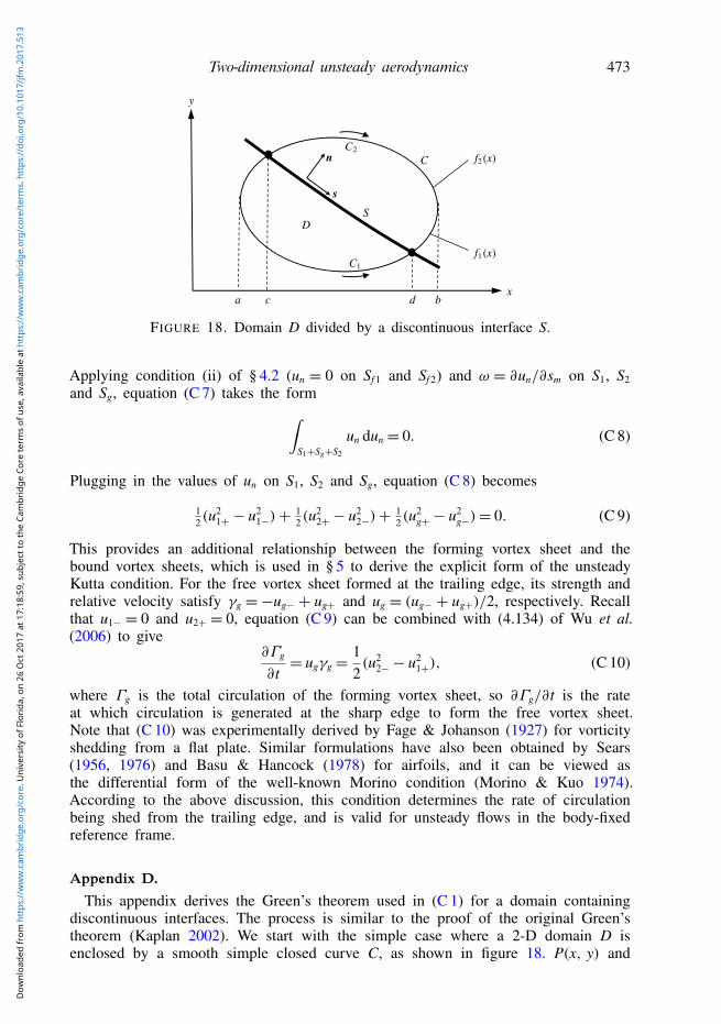
4.2. Momentum balance for a finite-angle trailing edgeWith the generalized sheet model proposed in § 4.1, we are now ready to derive themomentum balance for the merging flow at a finite-angle trailing edge, a schematicof which is provided in figure 4 with the main notations explained in table 2. Toformulate the problem, a 2-D material volume Am is defined in the body-fixedreference frame with its boundary ∂Am marked by the dashed contour. εs is thecharacteristic length of Am, and is defined as the length of the common interfaceSγ g between Am1 and Am2 as shown in figure 4. It is noted that the bulk of themerging area Am is immersed in the inviscid flow outside the sheet system. This isbecause the inviscid flow also plays an essential part in dictating the flow regimenear the trailing edge. In fact, for large Reynolds number situation, where mass andmomentum contributions from the viscous shear layer become negligible, the directionof the trailing-edge streamline should be solely governed by the inviscid flow. Here,a few physical assumptions and conditions are listed to simplify this problem.
(i) The merging process does not happen until the upper and lower streams meeteach other at the trailing edge, so any lead region of Am before the trailing edgeshould be much smaller than Am itself. To this end, the lengths of Sγ 1 and Sγ 2are assumed to be o(εs), whereas all other surfaces of Am, including S1, Sf 1, Sg−,Sg+, Sf 2 and S2, have dimension of O(εs).
(ii) Sf 1 and Sf 2 coincide with streamlines, so there is no mass flux across the surfacesand un = u · nm = 0.
(iii) Assuming the flow field changes smoothly, ∂/∂t of any quantity is finite.
To obtain the momentum balance equations, we start with the mass conservation.Note that the dividing surface Sγ g overlaps with the forming vortex sheet, so there isno mass flux across it and the mass conservation for Am can be written separately forAm1 and Am2 in the form
FIGURE 4. (Colour online) The formation of a free vortex sheet at a finite-angle trailingedge. The definitions of the main symbols are listed in table 2.
Am The control volume representing the merging area at a finite-angle trailingedge
Am1, Am2 The upper and lower volumes of Am, respectivelyS1, S2 The flow-entering boundaries of Am1 and Am2, respectivelySg+, Sg− The flow-exiting boundaries of Am1 and Am2, respectivelySf 1, Sf 2 The outer boundaries of Am1 and Am2, respectively, corresponding to
streamlinesSγ 1, Sγ 2 The inner boundaries of Am1 and Am2, respectively, on the surface of the
airfoilSγ g The common interface between Am1 and Am2
εs The length of the vortex sheet from the sharp corner to the end of thecontrol volume Am
∂Am The contour of Am surrounded by Sγ 1, S1, Sf 1, Sg−, Sg+, Sf 2, S2 and Sγ 2
sm, nm The unit tangential and normal vectors defined on ∂Am
sg, ng The unit tangential and normal vectors defined on the forming vortex sheetu1+, u2− The fluid-side velocities of the upper and lower bound vortex sheets,
respectivelyu1−, u2+ The solid-side velocities of the upper and lower bound vortex sheets,
respectivelyug−, ug+ The velocities at the upper and lower sides of the forming vortex sheet,
respectivelyγ1, γ2, γg Strengths of the upper and lower bound vortex sheets and the forming
vortex sheet, respectively
TABLE 2. Nomenclature table summarizing the main notations in figure 4.
For the bulk of Am, which contains incompressible isotropic Newtonian fluid, themomentum equation in the body-fixed reference frame is expressed as
dudt=
1ρ(−∇p+∇ · τ )+ uΩ, (4.11)
where τ is the shear stress tensor. Here, uΩ = −2Ω × u − Ω × (Ω × r) − Ub −
Ω × r, where Ub =−U represents the linear acceleration of the airfoil and U is thetranslational background flow velocity at the infinity in the body-fixed reference frame.Ω is the angular acceleration of the airfoil and r is the position vector relative to therotation centre. At this point, the momentum conservation for the whole Am can bederived as
ddt
∫Am
ρu dA =∫
Am
∂(ρu)∂t
dA+∮∂Am
ρu(u · nm) ds
=
∫Am−
(−∇p+∇ · τ + ρuΩ) dA
+
∫Sγ 1+Sγ 2+Sγ g
(JτK+∇ · T s) ds, (4.12)
where Sγ 1, Sγ 2 and Sγ g correspond to the vortex sheets in Am and Am− denotes the bulkof Am excluding Sγ 1, Sγ 2 and Sγ g. The first term in the second equation is obtainedby integrating equation (4.11), whereas the second term is derived from (4.4) with thepressure jump across a vortex sheet being zero.
Considering the infinitesimal size of the control volume normal to the vortex sheets,any variation of the velocity over S1, S2, Sg− and Sg+ is neglected. Together withcondition (ii) of this section, equations (4.9) and (4.10) can be further derived as
where the velocities associated with the vortex sheets (u1−, u1+, u2−, u2+, ug− and ug+)are normal to the surfaces of Am and are calculated from un= u · nm. The jump of thestreamfunction is applied here to account for the mass flux associated with a vortexsheet, similar to (4.1). And the mass flux associated with the forming vortex sheet isdivided into Jψg−K and Jψg−K by the trailing-edge streamline.
To simplify (4.12), we first apply conditions (i) and (iii) of the current section toargue that the integral associated with ∂(ρu)/∂t has magnitude O(ε2
s ). Physically, pis continuous so ∇p should be finite. Moreover, ∇ · τ = 0 holds for Am− becauseit corresponds to the inviscid flow outside the vortex sheets. Together with theboundedness of uΩ , equation (4.12) is reduced to∮
∂Am
u(u · nm) ds+O(ε2s )=
1ρ
∫Sγ 1+Sγ 2+Sγ g
(JτK+∇ · T s) ds. (4.15)
In the current study, there is no surface tension so ∇ · T s= 0. Sγ g corresponds to thefree vortex sheet which physically means JτK = 0. Furthermore, JτK is finite on thebound vortex sheets Sγ 1 and Sγ 2 according to (4.6). With condition (i), the right-handside of (4.15) becomes o(εs). Now, applying the velocity boundary conditions of ∂Am,
the momentum balance can be written in the sg and ng directions, respectively, in theform
(u21+S1 + Jψ1Ku∗1+) cos1θ1 + (u2
2−S2 + Jψ2Ku∗2+) cos1θ2
= u2g−Sg− + Jψg−Ku∗g− + u2
g+Sg+ + Jψg+Ku∗g+ +O(ε2s )+ o(εs), (4.16)
(u21+S1 + Jψ1Ku∗1+) sin1θ1
= (u22−S2 + Jψ2Ku∗2+) sin1θ2 +O(ε2
s )+ o(εs), (4.17)
where the superscript ∗ denotes the characteristic velocity scale based on themomentum flux of a vortex sheet, similar to (4.8).
In general, the JψK and u∗ terms need to be given or solved for an actual flow. Inthe current study, for the large Reynolds number situation, the mass and momentumassociated with the vortex sheet are neglected as a first approximation. So the JψKand u∗ terms become zero in (4.13), (4.14), (4.16) and (4.17). Furthermore, the termsO(ε2
s ) and o(εs) can be neglected in the limit εs→ 0. So (4.17) gives 1θ1 ·1θ2 > 0.Since
1θ1 +1θ2 =1θ0, (4.18)
it yields 1θ1, 1θ2 > 0 which means that the direction of the forming vortex sheetshould vary between the two tangents of the trailing-edge surfaces. Now, we cancombine (4.13), (4.14), (4.16) and (4.17) and cancel S1, S2, Sg− and Sg+ to obtain
This gives the momentum balance at a finite-angle trailing edge for large Reynoldsnumber flow. Equation (4.19) offers another relation between the forming vortex sheet(ug+, ug−, 1θ1 and 1θ2) and the existing bound vortex sheets (u1+ and u2−). It willbe applied in the next section to solve γg, ug and θg of the forming vortex sheet.
5. Explicit form of Kutta condition for general unsteady flowThe forming vortex sheet at a finite-angle trailing edge has been related to its
connecting bound vortex sheets through (3.5) and (4.19). For bound vortex sheets,the no-slip boundary condition gives u1−= 0 and u2+= 0, so γ1= u1+ and γ2=−u2−.Thus, equation (3.5) takes the form
γg =−ug− + ug+ = u1+ cos1θ1 − u2− cos1θ2. (5.1)
So far, only two equations are provided while three unknowns, ug+, ug− and 1θ1 (or1θ2), need to be solved.
Here, we present an additional relationship between the forming vortex sheet andthe bound vortex sheets to close the equation system. Recognizing that in generalvorticity generation only happens at the fluid–solid interface and that the merging zoneAm behind the trailing edge is barely connected to the airfoil body, we hypothesizethat the total vorticity generation as fluid passing Am should approach zero in thelimiting case Am → 0. In other words, the total change of circulation in Am shouldequal zero, which can be interpreted as an extension of the Kelvin’s circulationtheorem. Physically, the vortex-sheet system near the trailing edge consists of twosurface-bounded vortex sheets and a free vortex sheet released to form the wake.Each of these vortex sheets can be considered as a material sheet advected followingits local velocity field. In this sense, the vorticity of the forming vortex sheet is
not ‘generated’ at the trailing edge, but is the result of vorticity advection of thesurface-bounded vortex sheets. To substantiate this hypothesis, a detailed derivationconsistent with the current framework is provided in appendix C, where (C 9) or(C 10) provides the desired relationship.
At this point, we are ready to solve the explicit form of the unsteady Kuttacondition using (5.1), (4.19) and (C 9). We first combine (C 9) and (5.1) to expressug− and ug+ in terms of u1+, u2−, 1θ1 and 1θ2. And the results can be furtherplugged into (4.19) to give
Since 1θ1, 1θ2 > 0, equation (5.2) has the simplified form
u1+ sin1θ1 − u2− sin1θ2 = 0. (5.3)
Again, because 1θ1, 1θ2 > 0 and 0 6 1θ0 < π, this equation indicates that u1+ andu2− cannot take different signs. In the current study of vortex shedding (ug−, ug+> 0),this further indicates u1+, u2−6 0 which means no backward flow. Finally, with (4.18),equation (5.3) becomes
1θ1 = cos−1
(u2
1+ + u23 − u2
2−
2u1+u3
), 1θ2 = cos−1
(u2
2− + u23 − u2
1+
2u2−u3
)for u1+, u2− < 0,
1θ1 = 0, 1θ2 =1θ0 for u2− = 0,
1θ1 =1θ0, 1θ1 = 0 for u1+ = 0,
(5.4)
where u3 = −√
u21+ + u2
2− + 2u1+u2− cos1θ0. Therefore, equation (5.4) analyticallydetermines the direction of the forming vortex sheet (θg) at the trailing edge. Thecurrent work is derived for the case where no backward flow is present at thetrailing edge; and for the special case of a flat plate it predicts the angle of thetrailing-edge streamline to be tangential to the plate, which is consistent with the‘full’ Kutta condition derived by Orszag & Crow (1970), Daniels (1978) for flatplates. Equation (5.4) can be plugged into (C 10) and (5.1) to obtain the analyticalvortex-sheet strength (γg) and relative velocity (ug). This closes the task of derivingthe explicit form of the unsteady Kutta condition based on the existing bound vortexsheets. The implementation of this condition will be presented in § 6.1. In theremaining part of this section, we shall discuss the significance of this work and itspotential extension to the leading-edge vortex-sheet formation on a smooth surface.
The classical Kutta condition requires the rear stagnation streamline of an airfoilto be attached to the sharp trailing edge. Physically, this means that flow cannot turnaround the sharp edge. For steady flow at the trailing edge, Poling & Telionis (1986)has summarized a number of conditions that are equivalent to this condition:
(i) Continuous pressure at the trailing edge.(ii) The velocity at the trailing edge is finite or zero.
(iii) The shedding of vorticity vanishes (γg = 0).(iv) The stagnation streamline bisects the wedge angle of the trailing edge (1θ1 =
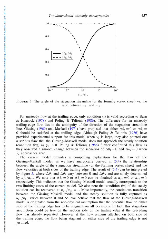
FIGURE 5. The angle of the stagnation streamline (or the forming vortex sheet) vs. theratio between u2− and u1+.
For unsteady flow at the trailing edge, only condition (i) is valid according to Basu& Hancock (1978) and Poling & Telionis (1986). The difference for an unsteadytrailing-edge flow lies in the ambiguity of the direction of the stagnation streamlineline. Giesing (1969) and Maskell (1971) have proposed that either 1θ1 = 0 or 1θ2 =
0 should be satisfied at the trailing edge. Although Poling & Telionis (1986) haveprovided experimental support for this model when γg is large, they also pointed outa serious flaw that the Giesing–Maskell model does not approach the steady solution(condition (iv)) as γg → 0. Poling & Telionis (1986) further confirmed this flaw asthey observed a smooth change between the scenarios of 1θ1 = 0 and 1θ2 = 0 whenγg approaches zero.
The current model provides a compelling explanation for the flaw of theGiesing–Maskell model, as we have analytically derived in (5.4) the relationshipbetween the angle of the stagnation streamline (or the forming vortex sheet) and theflow velocities at both sides of the trailing edge. The result of (5.4) can be interpretedby figure 5, where 1θ1 and 1θ2 vary between 0 and 1θ0, and are solely determinedby u2−/u1+. We note that 1θ1 = 0 or 1θ2 = 0 can be obtained as u2− = 0 or u1+ = 0,respectively. This indicates that the Giesing–Maskell model actually corresponds to thetwo limiting cases of the current model. We also note that condition (iv) of the steadysolution can be recovered at u2−/u1+ = 1. Most importantly, the continuous transitionbetween the Giesing–Maskell model and the steady solution is fully captured asu2−/u1+ varies between 0 and ∞. We believe that the flaw of the Giesing–Maskellmodel is originated from the non-physical assumption that the potential flow on eitherside of the trailing edge has to be stagnant on all occasions. In fact, this stagnationassumption could be true on the suction side of the trailing edge if the precedingflow has already separated. However, if the flow remains attached on both side ofthe trailing edge, the flow being stagnant on either side of the trailing edge is notjustified.
FIGURE 6. (Colour online) The structure of viscous sheer layers and the correspondingvortex sheets near a flow separation point on a smooth surface. It is noted that u2+ =
u2− = 0 and γ2 = 0.
The current model for the trailing-edge vortex sheet is based on conservationlaws and the unsteady Kutta condition which only requires a continuous pressuredistribution. In this sense, there should not be any fundamental difference for theformation of a vortex sheet due to flow separation on a smooth surface. Thus, wefurther propose to extend this model to deciding the formation of a leading-edgevortex sheet. For this purpose, the separated vortex sheet can be viewed as beinggenerated due to the merging of the two bound vortex sheets at both sides of theseparation point. Considering the actual viscous shear layers near a separation pointas shown in figure 6, the downstream-side shear layer consists of a reverse-flowlayer and a separated-flow layer. In the vortex-sheet limit, the reverse-flow layerbecomes the bound vortex sheet while the separated-flow layer becomes the separatedvortex sheet. Apparently, the velocities at both sides of the reverse-flow layer arezero (u2+ = u2− = 0), meaning the corresponding bound vortex-sheet strength is zero(γ2 = 0) near the separation point. Based on the above discussions, we can attributethe formation of the separated vortex sheet to the scenario of the Giesing–Maskellmodel. Because 1θ0 = π for a smooth surface, we immediately obtain 1θ1 = 0 and1θ2 = π, which means that the forming vortex sheet from a separation point of asmooth surface should be tangential to the surface. Finally, applying (C 10) and (5.1)gives the strength and velocity of the forming vortex sheet, which are actually equalto the values of its upstream bound vortex sheet (γg = γ1 and ug = u1+/2).
6. Simulations and validationsTo verify the unsteady flow model together with the vortex-sheet formation
conditions for a 2-D airfoil, this section will simulate different airfoils in steadyand unsteady background flows, and then compare the results with experimental dataor empirical models. Here, we note that the formation of the leading-edge vortexsheet at large angle of attack (AoA) requires predicting the leading-edge separationpoint, which could be a topic of a future investigation. Furthermore, equation (5.4)implies that the current unsteady Kutta condition applies to the situation where nobackward flow presents at the trailing edge. This means that the model does notaccount for any separation happening before the trailing edge, which would likely tooccur for highly unsteady flows. To this end, the following assumes fully attachedflow and vortex shedding only at the trailing edge. For this reason, the applicationsof this study are limited to small-to-medium AoA regimes, where the flow might beconsidered to remain attached without losing much accuracy.
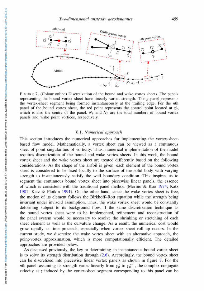
FIGURE 7. (Colour online) Discretization of the bound and wake vortex sheets. The panelsrepresenting the bound vortex sheet have linearly varied strength. The g panel representsthe vortex-sheet segment being formed instantaneously at the trailing edge. For the nthpanel of the bound vortex sheet, the red point represents the control point located at zn
C,which is also the centre of the panel. NB and NT are the total numbers of bound vortexpanels and wake point vortices, respectively.
6.1. Numerical approach
This section introduces the numerical approaches for implementing the vortex-sheet-based flow model. Mathematically, a vortex sheet can be viewed as a continuoussheet of point singularities of vorticity. Thus, numerical implementation of the modelrequires discretization of the bound and wake vortex sheets. In this work, the boundvortex sheet and the wake vortex sheet are treated differently based on the followingconsiderations. As the shape of the airfoil is given, each element of the bound vortexsheet is considered to be fixed locally to the surface of the solid body with varyingstrength to instantaneously satisfy the wall boundary condition. This inspires us tosegment the continuous bound vortex sheet into piecewise linear panels, the essenceof which is consistent with the traditional panel method (Morino & Kuo 1974; Katz1981; Katz & Plotkin 1991). On the other hand, since the wake vortex sheet is free,the motion of its element follows the Birkhoff–Rott equation while the strength beinginvariant under inviscid assumption. Thus, the wake vortex sheet would be constantlydeforming subject to its background flow. If the same discretization technique asthe bound vortex sheet were to be implemented, refinement and reconstruction ofthe panel system would be necessary to resolve the shrinking or stretching of eachsheet element as well as the curvature change. As a result, the numerical cost wouldgrow rapidly as time proceeds, especially when vortex sheet roll up occurs. In thecurrent study, we discretize the wake vortex sheet with an alternative approach, thepoint-vortex approximation, which is more computationally efficient. The detailedapproaches are provided below.
As discussed previously, the key to determining an instantaneous bound vortex sheetis to solve its strength distribution through (2.6). Accordingly, the bound vortex sheetcan be discretized into piecewise linear vortex panels as shown in figure 7. For thenth panel, assuming its strength varies linearly from γ n
B to γ n+1B , the complex-conjugate
velocity at z induced by the vortex-sheet segment corresponding to this panel can be
B). For an instantaneous flow, the only unknownparameters are the strengths γ n
B and γ n+1B associated with each vortex panel.
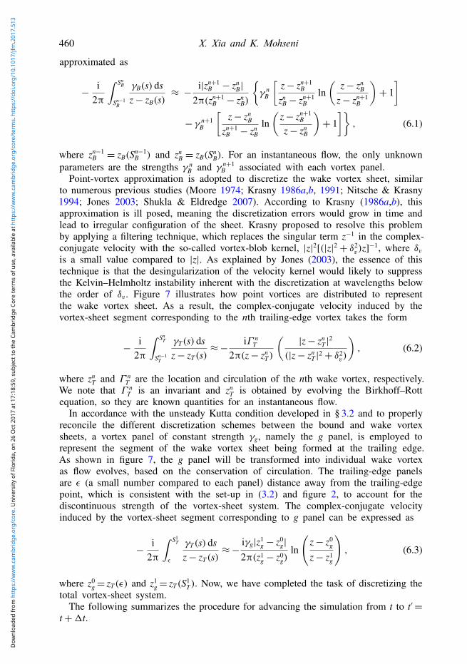
Point-vortex approximation is adopted to discretize the wake vortex sheet, similarto numerous previous studies (Moore 1974; Krasny 1986a,b, 1991; Nitsche & Krasny1994; Jones 2003; Shukla & Eldredge 2007). According to Krasny (1986a,b), thisapproximation is ill posed, meaning the discretization errors would grow in time andlead to irregular configuration of the sheet. Krasny proposed to resolve this problemby applying a filtering technique, which replaces the singular term z−1 in the complex-conjugate velocity with the so-called vortex-blob kernel, |z|2[(|z|2 + δ2
v)z]−1, where δv
is a small value compared to |z|. As explained by Jones (2003), the essence of thistechnique is that the desingularization of the velocity kernel would likely to suppressthe Kelvin–Helmholtz instability inherent with the discretization at wavelengths belowthe order of δv. Figure 7 illustrates how point vortices are distributed to representthe wake vortex sheet. As a result, the complex-conjugate velocity induced by thevortex-sheet segment corresponding to the nth trailing-edge vortex takes the form
−i
2π
∫ SnT
Sn−1T
γT(s) dsz− zT(s)
≈−iΓ n
T
2π(z− znT)
(|z− zn
T |2
(|z− znT |
2 + δ2v)
), (6.2)
where znT and Γ n
T are the location and circulation of the nth wake vortex, respectively.We note that Γ n
T is an invariant and znT is obtained by evolving the Birkhoff–Rott
equation, so they are known quantities for an instantaneous flow.In accordance with the unsteady Kutta condition developed in § 3.2 and to properly
reconcile the different discretization schemes between the bound and wake vortexsheets, a vortex panel of constant strength γg, namely the g panel, is employed torepresent the segment of the wake vortex sheet being formed at the trailing edge.As shown in figure 7, the g panel will be transformed into individual wake vortexas flow evolves, based on the conservation of circulation. The trailing-edge panelsare ε (a small number compared to each panel) distance away from the trailing-edgepoint, which is consistent with the set-up in (3.2) and figure 2, to account for thediscontinuous strength of the vortex-sheet system. The complex-conjugate velocityinduced by the vortex-sheet segment corresponding to g panel can be expressed as
−i
2π
∫ S1T
ε
γT(s) dsz− zT(s)
≈−iγg|z1
g − z0g|
2π(z1g − z0
g)ln
(z− z0
g
z− z1g
), (6.3)
where z0g= zT(ε) and z1
g= zT(S1T). Now, we have completed the task of discretizing the
total vortex-sheet system.The following summarizes the procedure for advancing the simulation from t to t′=
Step 1: Wake evolution. By the end of the previous step, the flow field is solved,so zn
B(t), γnB (t), zn
T(t), Γn
T (t), z1g(t) and γg(t) are known variables. To obtain the wake
distribution for the new step, the g panel is first replaced by a new point vortex using
zNT+1T (t′)= (z0
g(t)+ z1g(t))/2, (6.4)
Γ NT+1T (t′)= γg(t)|z1
g(t)− z0g(t)|, (6.5)
where the latter is essentially the conservation of circulation. Then, znT(t′) of each wake
vortex is evolved by integrating the Birkhoff–Rott equation with a fourth-order Runge-Kutta scheme.
Step 2: Motion update. Since the motion of the airfoil is prescribed in this study, thetranslational and rotational motions of the airfoil, U(t′) and Ω(t′), need to be updated.If the airfoil is deformable, updating zn
B(t′) is also necessary.
Step 3: g panel addition. The new g panel at t′ should be added based on theproposed unsteady Kutta condition. This requires a full knowledge of its connectingbound vortex panels at t′, which are yet to be computed. Here, the bound vortexpanels together with the g panel are solved in a coupled sense. To avoid nonlinearityin solving this coupled system, the direction θg(t′) and shedding velocity ug(t′) of theg panel are computed from (5.4), (5.1) and (C 10), based on the bound vortex panelsof the previous time step. Consequently, z1
g(t′) can be decided from
z1g(t′)= zTE + (ε + ug(t′)1t)eiθg(t′), (6.6)
where zTE is the complex coordinate of the trailing edge point.
Step 4: Equation solving. At this stage, the unknown variables are the strengths ofthe bound vortex panels and the g panel. In figure 7, zn
C marks the control pointwhere the wall boundary condition is satisfied for each panel. Applying the velocityapproximations of (6.1), (6.2) and (6.3), the boundary condition specified by (2.5)and (2.6) can be written in the form,
NB+1∑m=1
DnmγmB + Enγg =Hn, n= 1, 2, . . . ,NB, (6.7)
where Dnm, En and Hn are coefficients or constants expressed by znC and other known
parameters. For brevity, their detailed expressions are not presented. Furthermore, theKelvin’s circulation theorem predicts that all vortices in the flow field should satisfy
12
NB∑m=1
|zm+1B − zm
B |γmB +
12
NB+1∑m=2
|zmB − zm−1
B |γmB + |z
1g − z0
g|γg =−
NT∑m=1
Γ mT . (6.8)
Therefore, equations (6.7), (6.8) and (3.5) together constitute a (NB+ 2)th-order linearsystem, which is solved analytically to give [γ 1
Bγ2B . . . γ
NB+1B γg]
T. This completes thecomputation of the entire vortex-sheet system at time t′. Last, for flow initializationat t= 0, step 4 should be performed with γg= 0 and NT
= 0, so the (NB+ 1)th-orderlinear system of the combined equations (6.7) and (6.8) is solved to give the initialstrength distribution of the bound vortex sheet.
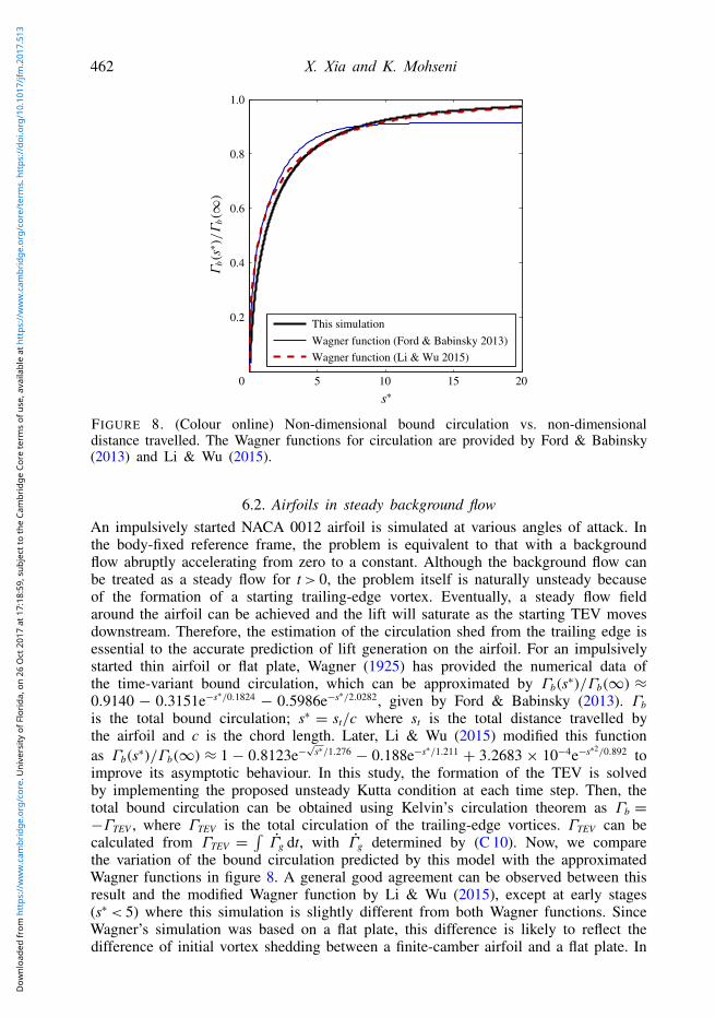
FIGURE 8. (Colour online) Non-dimensional bound circulation vs. non-dimensionaldistance travelled. The Wagner functions for circulation are provided by Ford & Babinsky(2013) and Li & Wu (2015).
6.2. Airfoils in steady background flowAn impulsively started NACA 0012 airfoil is simulated at various angles of attack. Inthe body-fixed reference frame, the problem is equivalent to that with a backgroundflow abruptly accelerating from zero to a constant. Although the background flow canbe treated as a steady flow for t> 0, the problem itself is naturally unsteady becauseof the formation of a starting trailing-edge vortex. Eventually, a steady flow fieldaround the airfoil can be achieved and the lift will saturate as the starting TEV movesdownstream. Therefore, the estimation of the circulation shed from the trailing edge isessential to the accurate prediction of lift generation on the airfoil. For an impulsivelystarted thin airfoil or flat plate, Wagner (1925) has provided the numerical data ofthe time-variant bound circulation, which can be approximated by Γb(s∗)/Γb(∞) ≈
0.9140 − 0.3151e−s∗/0.1824− 0.5986e−s∗/2.0282, given by Ford & Babinsky (2013). Γb
is the total bound circulation; s∗ = st/c where st is the total distance travelled bythe airfoil and c is the chord length. Later, Li & Wu (2015) modified this functionas Γb(s∗)/Γb(∞) ≈ 1 − 0.8123e−
√s∗/1.276
− 0.188e−s∗/1.211+ 3.2683 × 10⁻⁴e−s∗2/0.892 to
improve its asymptotic behaviour. In this study, the formation of the TEV is solvedby implementing the proposed unsteady Kutta condition at each time step. Then, thetotal bound circulation can be obtained using Kelvin’s circulation theorem as Γb =
−ΓTEV , where ΓTEV is the total circulation of the trailing-edge vortices. ΓTEV can becalculated from ΓTEV =
∫Γg dt, with Γg determined by (C 10). Now, we compare
the variation of the bound circulation predicted by this model with the approximatedWagner functions in figure 8. A general good agreement can be observed between thisresult and the modified Wagner function by Li & Wu (2015), except at early stages(s∗ < 5) where this simulation is slightly different from both Wagner functions. SinceWagner’s simulation was based on a flat plate, this difference is likely to reflect thedifference of initial vortex shedding between a finite-camber airfoil and a flat plate. In
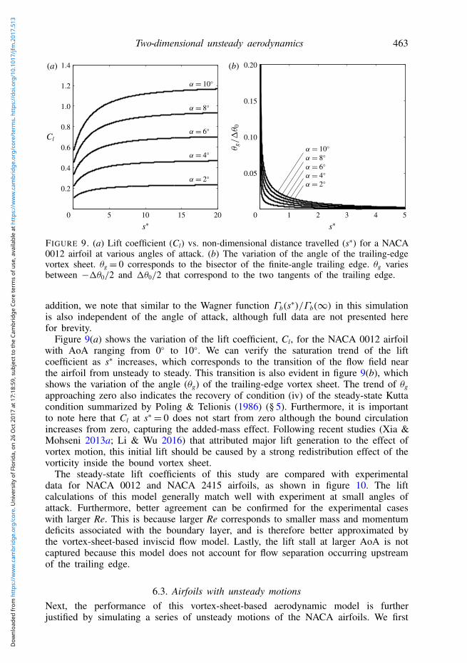
FIGURE 9. (a) Lift coefficient (Cl) vs. non-dimensional distance travelled (s∗) for a NACA0012 airfoil at various angles of attack. (b) The variation of the angle of the trailing-edgevortex sheet. θg = 0 corresponds to the bisector of the finite-angle trailing edge. θg variesbetween −1θ0/2 and 1θ0/2 that correspond to the two tangents of the trailing edge.
addition, we note that similar to the Wagner function Γb(s∗)/Γb(∞) in this simulationis also independent of the angle of attack, although full data are not presented herefor brevity.
Figure 9(a) shows the variation of the lift coefficient, Cl, for the NACA 0012 airfoilwith AoA ranging from 0 to 10. We can verify the saturation trend of the liftcoefficient as s∗ increases, which corresponds to the transition of the flow field nearthe airfoil from unsteady to steady. This transition is also evident in figure 9(b), whichshows the variation of the angle (θg) of the trailing-edge vortex sheet. The trend of θgapproaching zero also indicates the recovery of condition (iv) of the steady-state Kuttacondition summarized by Poling & Telionis (1986) (§ 5). Furthermore, it is importantto note here that Cl at s∗= 0 does not start from zero although the bound circulationincreases from zero, capturing the added-mass effect. Following recent studies (Xia &Mohseni 2013a; Li & Wu 2016) that attributed major lift generation to the effect ofvortex motion, this initial lift should be caused by a strong redistribution effect of thevorticity inside the bound vortex sheet.
The steady-state lift coefficients of this study are compared with experimentaldata for NACA 0012 and NACA 2415 airfoils, as shown in figure 10. The liftcalculations of this model generally match well with experiment at small angles ofattack. Furthermore, better agreement can be confirmed for the experimental caseswith larger Re. This is because larger Re corresponds to smaller mass and momentumdeficits associated with the boundary layer, and is therefore better approximated bythe vortex-sheet-based inviscid flow model. Lastly, the lift stall at larger AoA is notcaptured because this model does not account for flow separation occurring upstreamof the trailing edge.
6.3. Airfoils with unsteady motionsNext, the performance of this vortex-sheet-based aerodynamic model is furtherjustified by simulating a series of unsteady motions of the NACA airfoils. We first
FIGURE 10. (Colour online) Lift coefficient (Cl) vs. angle of attack (α) for (a) a NACA0012 airfoil and (b) a NACA 2415 airfoil. The experimental data for (a) and (b) are fromSheldahl & Klimas (1981) and Abbott, von Doenhoff & Stivers (1945), respectively.
Experiment This simulation(a) (b)
FIGURE 11. (Colour online) Comparison between flow visualization and simulation for apitching and heaving NACA 0012 airfoil with St= 0.45, αmax = 30 and h0 = 0.75c. Theflow visualization image is from Schouveiler, Hover & Triantafyllou (2005). The dash linein (b) marks the trajectory of the airfoil.
investigate a NACA 0012 airfoil with a combined pitching and heaving motionadapted from the experiment of Read, Hover & Triantafyllou (2003). For all tests,the chord length and the towing speed are fixed at c= 0.1 m and Utow = 0.4 m s−1,respectively. The corresponding Reynolds number is 4 × 10⁴. The pivot for thepitching motion is fixed at 1/3 chord. The phase difference angle between thepitching and heaving motions is set to 90. The characteristic parameters for thismotion are the Strouhal number, St, the amplitude of the angle of attack, αmax, andthe heave amplitude, h0, which could be adjusted by controlling the pitching andheaving motions. Figure 11 compares the wake structures between this simulationand the flow visualization for a sample case (St = 0.45, αmax = 30 and h0 = 0.75c).The matching of the wake patterns between experiment and simulation is promising.Figure 12 further plots the instantaneous force vectors along the trajectories oftwo different pitching and heaving motions. The results demonstrate reasonableagreement of the force magnitude and direction between experiment and simulation.This quantitatively validates the performance of the aerodynamic model and the TEV
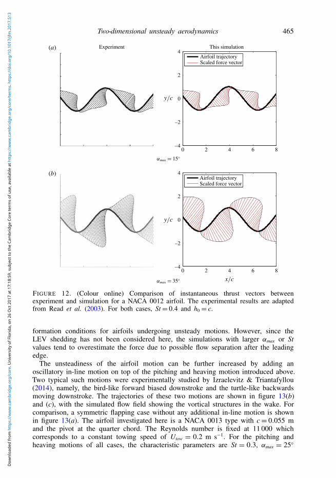
FIGURE 12. (Colour online) Comparison of instantaneous thrust vectors betweenexperiment and simulation for a NACA 0012 airfoil. The experimental results are adaptedfrom Read et al. (2003). For both cases, St= 0.4 and h0 = c.
formation conditions for airfoils undergoing unsteady motions. However, since theLEV shedding has not been considered here, the simulations with larger αmax or Stvalues tend to overestimate the force due to possible flow separation after the leadingedge.
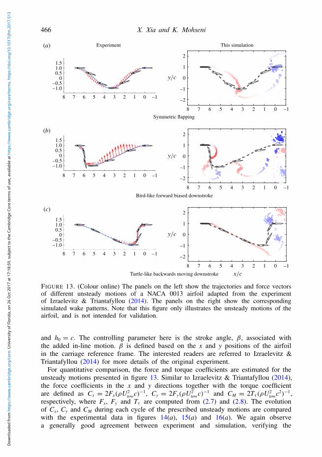
The unsteadiness of the airfoil motion can be further increased by adding anoscillatory in-line motion on top of the pitching and heaving motion introduced above.Two typical such motions were experimentally studied by Izraelevitz & Triantafyllou(2014), namely, the bird-like forward biased downstroke and the turtle-like backwardsmoving downstroke. The trajectories of these two motions are shown in figure 13(b)and (c), with the simulated flow field showing the vortical structures in the wake. Forcomparison, a symmetric flapping case without any additional in-line motion is shownin figure 13(a). The airfoil investigated here is a NACA 0013 type with c= 0.055 mand the pivot at the quarter chord. The Reynolds number is fixed at 11 000 whichcorresponds to a constant towing speed of Utow = 0.2 m s−1. For the pitching andheaving motions of all cases, the characteristic parameters are St = 0.3, αmax = 25
FIGURE 13. (Colour online) The panels on the left show the trajectories and force vectorsof different unsteady motions of a NACA 0013 airfoil adapted from the experimentof Izraelevitz & Triantafyllou (2014). The panels on the right show the correspondingsimulated wake patterns. Note that this figure only illustrates the unsteady motions of theairfoil, and is not intended for validation.
and h0 = c. The controlling parameter here is the stroke angle, β, associated withthe added in-line motion. β is defined based on the x and y positions of the airfoilin the carriage reference frame. The interested readers are referred to Izraelevitz &Triantafyllou (2014) for more details of the original experiment.
For quantitative comparison, the force and torque coefficients are estimated for theunsteady motions presented in figure 13. Similar to Izraelevitz & Triantafyllou (2014),the force coefficients in the x and y directions together with the torque coefficientare defined as Cx = 2Fx(ρU2
towc)−1, Cy = 2Fy(ρU2towc)−1 and CM = 2Tτ (ρU2
towc2)−1,respectively, where Fx, Fy and Tτ are computed from (2.7) and (2.8). The evolutionof Cx, Cy and CM during each cycle of the prescribed unsteady motions are comparedwith the experimental data in figures 14(a), 15(a) and 16(a). We again observea generally good agreement between experiment and simulation, verifying the
FIGURE 14. (Colour online) Result of the symmetric flapping motion correspondingto figure 13(a). (a) Comparison between the measured force coefficients of Izraelevitz& Triantafyllou (2014) and the estimated force coefficients from this simulation. (b)Variations of α, U and θg during one cycle.
5
0
–5
t
10
0.5
0
–0.5
–1.0
1.0
1.5
2.0(a) (b)
t
Forc
e co
effi
cien
ts
FIGURE 15. (Colour online) Result of the bird-like forward biased downstrokecorresponding to figure 13(b). (a) Comparison between measured and estimated forcecoefficients. (b) Variations of α, U and θg during one cycle.
performance of the proposed flow model. Especially, the results of Cy have promisingaccuracy for all three different cases. Since Cy physically represents the lift coefficient,this indicates a prospective application of the current model for lift estimation withoutmodelling the leading-edge separation. However, the void of flow separation in thecurrent simulation seems to have a notable impact on Cx, which corresponds tothe thrust coefficient. This is reflected by the over-prediction of Cx in some casesdisplayed in figures 14(a) and 15(a). Other than the flow separation, the viscouseffect at the solid–fluid interface could also affect the accuracy of predicting thrustor drag using an inviscid flow model.
FIGURE 16. (Colour online) Result of the turtle-like backwards moving downstrokecorresponding to figure 13(c). (a) Comparison between measured and estimated forcecoefficients. (b) Variations of α, U and θg during one cycle.
To explain the effect of the additional in-line motion on force generation of theairfoil, the variations of the airfoil velocity U and the angle of attack α are plotted infigures 14(b), 15(b) and 16(b). We can observe that the variations of α in figures 15and 16 are identical, and α only changes in the first half-cycle while it remains zeroin the second half-cycle. Since the shedding of strong vorticity mainly occurs at non-zero angles of attack, the force generation associated with vortex shedding shouldmostly happen during the first half-cycle. In this sense, the first half-cycle is theactual ‘stroke’ while the second half can be considered as the ‘recovery’. However,the different in-line motions during the first half-cycle cause U to increase significantlyfor the bird-like downstroke in figure 15 and decrease significantly for the turtle-likedownstroke in figure 16. This creates stronger and faster trailing-edge vortices of thebird-like downstroke compared to the turtle-like downstroke. As a result, the bird-likedownstroke provides much higher lift than the turtle-like downstroke. Finally, we notethat the angle of the trailing-edge vortex sheet, θg, varies smoothly within the limitsof the two tangential directions of the trailing edge, −1θ0/2 and 1θ0/2. This alsoimplies the correct implementation of the proposed models, and is in accordance withthe experimental observation of Poling & Telionis (1986) that the direction of thetrailing-edge streamline changes smoothly.
7. Conclusions
An unsteady aerodynamic model for an airfoil was derived based on the dynamicsof the bound vortex sheet and the wake vortices. The vorticity generation mechanismat the trailing edge was studied since it is essential to predict the vortex shedding andevolution processes in the wake. For a flat plate or a cusped trailing edge, this canbe solved by applying an unsteady Kutta condition, based on the physical sense thatflow cannot turn around a sharp edge. The current work extended this condition toa more general situation, the finite-angle trailing edge of an airfoil, by enforcing theflow direction at the trailing edge to be tangential to the forming vortex sheet. This
resulted in an implicit Kutta condition which relates the strength of the forming vortexsheet to its adjacent bound vortex sheets.
This unsteady Kutta condition is not straightforward to implement because it alsodepends on the direction of the forming vortex sheet, which is ambiguous for afinite-angle trailing edge. To address this problem, this study proposed a generalizedsheet model to enable momentum balance analysis for the vortex-sheet system and itssurrounding flow at the trailing edge. The essence of the generalized sheet model isthat a physical viscous shear layer could be adequately represented by a vortex sheetif the dynamics is captured by relevant global quantities. Specifically, the modellingof mass and momentum fluxes through jump conditions would allow the estimationsof entrainment and viscous force of the original shear layer in an inviscid flow. Theapplication of this model in the case of the finite-angle trailing edge provided anotherimplicit relation between the forming vortex sheet and the existing bound vortexsheets.
The combination of the implicit unsteady Kutta condition and the momentumbalance equation, together with the conservation of circulation, gave the analyticalexpression of the angle, strength and shedding velocity of a free vortex sheet formedat a finite-angle trailing edge, establishing a general unsteady Kutta condition forrelevant problems. The significance of this work is that the vortex-sheet formationcondition allows the angle of the forming vortex sheet to continuously changebetween the two tangents of the trailing edge. This resolves the paradox of theGiesing–Maskell model that it does not converge to the steady-state Kutta condition.Airfoils in various steady and unsteady flows were simulated and the resulting flowfield and force calculations were compared with experimental data. The promisingagreement between simulation and experiment confirmed the validity of the proposedunsteady Kutta condition as well as the vortex-sheet-based aerodynamic model.
Acknowledgements
This work is partially supported by a grant from the Office of Naval Research. Wewould like to thank Dr. A. DeVoria for providing helpful discussions and comments.We also appreciate the reviewers’ valuable comments that led to great improvementsof this paper.
Appendix A.
This appendix, together with appendix B, provides the detailed calculation for (3.4).In this study, we are faced with the task of computing the line integral
∫γ (s)(Z0 −
Z(s))−1 ds between two different points, Z(a) and Z(b) (0 < a < b), along a simpleopen (without self-intersection) curve, C1, which starts from Z0 in the complex domain,as shown in figure 17. s is the curve length between Z0 and an arbitrary point Z(s)on C1, so Z0 = Z(0). γ (s) is a real function defined on curve C1. Given C1 andγ (s) are smooth (class C∞) for a 6 s 6 b, it means that Z(s) and γ (s) are infinitelydifferentiable on Cab = Z(s), a 6 s 6 b.
Since γ (s) is infinitely differentiable for a 6 s 6 b, it can be expanded to Taylorseries at s= a:
FIGURE 17. (Colour online) A diagram of the curve C1 for calculating the integral∫γ (s)(Z0 − Z(s))−1 ds.
Plugging in (A 1), the objective integral takes the form
Iab =
∫Cab
γ (s) dsZ0 − Z(s)
=
∫Cab
∞∑n=0
gn(s− a)n
Z0 − Z(s)ds. (A 2)
As the series∑∞
n=0 gn(s − a)n converges uniformly on the interval [a, b], we caninterchange summation and integration in (A 2) to obtain the series,
Iab =
∞∑n=0
gn
∫Cab
(Z0 − Z(s))−1(s− a)n ds. (A 3)
Let In denote the nth term of the series in (A 3). With Z(s) being infinitelydifferentiable on [a, b], we may substitute (Z0 − Z(s))−1 in (A 3) with a Taylorseries and then integrate to show that In is O((b − a)n+1) as (b − a) → 0. Thus,In+1 = o(In) as (b− a)→ 0 which qualifies
∑∞
n=0 In as an asymptotic expansion.At this point, for small b − a the original integral can be approximately by the
zeroth-order term,
I0 = g0
∫Cab
(Z0 − Z(s))−1 ds= g0
∫Cab
ds/dzZ0 − z
dz, (A 4)
where z= Z(s) for z ∈Cab. Dz(s)= ds/dz can be expanded to Taylor series,
Dz(s)=∞∑
m=0
fzm(s− a)m where fzm =D(m)
z (a)m!
. (A 5)
So (A 4) can be derived as,
I0 = g0
∞∑m=0
fzm
∫Cab
(s− a)m
Z0 − zdz
=
∞∑m=0
g0fzm
[(−ln(Z0 − z)(s− a)m)|Z(b)Z(a) +
∫Cab
ln(Z0 − z)m(s− a)m−1 ds], (A 6)
where the second equation is obtained using integration by parts. Let Rm denote themth term of the series in (A 6). It can be readily verified that the first part of Rm isO((b− a)m) as (b− a)→ 0. For the second part, its magnitude can be shown to beO((b − a)m), by expanding ln(Z0 − z) to Taylor series and then applying integration.
n=0 In, we can now show that Rm+1 = o(Rm)as (b− a)→ 0, which indicates
∑∞
m=0 Rm is an asymptotic expansion. Its zeroth-orderterm takes the form,
R0 =−g0fz0 ln(
Z0 − Z(b)Z0 − Z(a)
), (A 7)
where g0 = γ (a) and fz0 = (dz/ds)−1|s=a = e−iθa . Moreover, the leading-order terms for
Z0 − Z(b) and Z0 − Z(a) are estimated to be −beiθa and −aeiθa , respectively. In theproblem of interest, we are concerned with the limiting case where Z(a)→Z0 or a→0. So ln(b)= o(ln(a)) and Iab can be simplified as
lima→0
Iab = γ (a)e−iθa ln(a)+ o(ln(a)). (A 8)
In this way, the objective integral is approximated by the leading-order term of theasymptotic expansion. It is noted that the nature of the asymptotic expansion requiresb− a to be sufficiently small.
Appendix B.This appendix is a continuation of appendix A. Appendix A has calculated the
integral∫γ (s)(Z0−Z(s))−1 ds between Z(a) and Z(b) for the limiting case Z(a)→Z0.
In this part, the goal is to prove that the objective integral is bounded if a is a finitevalue or Z(a) is away from Z0.
For this purpose, we only require γ (s) to be bounded for a 6 s 6 b. Let Dm =
min|Z − Z0|, Z ∈ Cab and γM = maxγ (s), s ∈ [a, b], the objective integral has theinequality∣∣∣∣∫
Cab
γ (s) dsZ0 − Z(s)
∣∣∣∣6 ∫Cab
∣∣∣∣ 1Z0 − Z(s)
∣∣∣∣ |γ (s)| ds<∫
Cab
γM
Dmds=
γM(b− a)Dm
. (B 1)
This completes the proof for the boundedness of the objective integral.
Appendix C.The objective of this appendix is to derive Kelvin’s circulation theorem for the
trailing-edge merging zone Am shown in figure 4. We begin by expressing the totalchange of the circulation within Am as
ddt
∫Am
ω dA=ddt
∮∂Am
u · sm ds=∮∂Am
dudt· sm ds+
∮∂Am
12
d(u · u), (C 1)
where ω is the vorticity. The left-hand equation is based on the Green theorem. Sincea vortex sheet corresponds to a velocity discontinuity, the Green theorem should bederived for a volume containing discontinuous surfaces as presented in appendix D.We note that since the velocity derivative across a vortex sheet satisfies the Diracdelta function specified in (D 5), the Green theorem should take its original form. Inthe right equation, since u is a Heaviside step function across any vortex sheet, it issingle valued throughout the entire domain. So the second term on the right-hand sideof (C 1) is equal to zero. Now, we plug the momentum equation (4.11) into (C 1) toobtain
This gives a general equation for the total change of circulation inside Am. Now, weapply physical boundary conditions to simplify (C 2). Since Sγ 1 and Sγ 2 correspond tofluid–solid interfaces that satisfy the no-slip boundary condition, we obtain du/dt= 0in the body-fixed reference frame. Furthermore, the flow outside the vortex sheets areassumed to be inviscid, so we have ∇ · τ = 0 on the other boundaries ∂Am− Sγ 1− Sγ 2.Therefore, equation (C 2) becomes
ddt
∫Am
ω dA=∫∂Am−Sγ 1−Sγ 2
(−∂pρ∂sm
+ uΩ · sm
)ds. (C 3)
Under condition (iii) of § 4.2, uΩ · sm should be finite. Together with condition (i), thesecond integral of (C 3) has the magnitude O(εs). So (C 3) has the simplified form
ddt
∫Am
ω dA=−1ρ
∫∂Am−Sγ 1−Sγ 2
dp+O(εs). (C 4)
Let p1 and p2 be the pressure of the points shown in figure 4, the result of (C 4)becomes (p2− p1)/ρ+O(εs). Physically, pressure should be continuous at the trailingedge which means p1 = p2 as εs→ 0. Therefore, equation (C 4) becomes zero in thelimit εs→ 0, which gives Kelvin’s circulation theorem.
On the other hand, vorticity can be viewed as a material quantity moving with afluid element. So the total change of circulation inside Am can be expressed using theReynolds transport theorem as
ddt
∫Am
ω dA=∫
Am
∂ω
∂tdA+
∮∂Am
ω(u · nm) ds. (C 5)
The first term on the right-hand side of (C 5) can be derived as∫Am
∂ω
∂tdA=
∂
∂t
∫Am
ω dA=∂γm
∂tLm, (C 6)
where γm and Lm represent the effective strength and length of the total vortex-sheetsystem inside Am, respectively. Again, ∂γm/∂t should be finite according to condition(iii) of § 4.2. Condition (i) gives Lm∼O(εs), so (C 6) also approaches zero in the limitεs→ 0. Together with (C 4) being zero as εs→ 0, equation (C 5) is reduced to∮
∂Am
ω(u · nm) ds= 0. (C 7)
Now, the vorticity is defined as ω = ∂un/∂sm − ∂us/∂nm on S1, S2 and Sg. Since thetangential directions of the vortex sheets, γ1, γ2 and γg, are normal to S1, S2 and Sg,respectively, sm and nm are actually n and s in the s− n coordinate defined locally oneach vortex sheet. For a physical shear layer, the boundary layer approximation couldbe applied so |∂/∂n| |∂/∂s| in the s− n coordinate. This is translated into |∂/∂sm|
|∂/∂nm| in the sm − nm coordinate. Thus, |∂un/∂sm| |∂un/∂nm| and |∂us/∂sm|
|∂us/∂nm|. Together with the continuity equation, ∂us/∂sm + ∂un/∂nm = 0, it gives|∂un/∂sm| |∂us/∂nm|. This means that the ∂us/∂nm term has a negligible contributionin the vorticity expression and is dropped in the following derivation for simplicity.
FIGURE 18. Domain D divided by a discontinuous interface S.
Applying condition (ii) of § 4.2 (un = 0 on Sf 1 and Sf 2) and ω = ∂un/∂sm on S1, S2and Sg, equation (C 7) takes the form∫
S1+Sg+S2
un dun = 0. (C 8)
Plugging in the values of un on S1, S2 and Sg, equation (C 8) becomes
12(u
21+ − u2
1−)+12(u
22+ − u2
2−)+12(u
2g+ − u2
g−)= 0. (C 9)
This provides an additional relationship between the forming vortex sheet and thebound vortex sheets, which is used in § 5 to derive the explicit form of the unsteadyKutta condition. For the free vortex sheet formed at the trailing edge, its strength andrelative velocity satisfy γg =−ug− + ug+ and ug = (ug− + ug+)/2, respectively. Recallthat u1− = 0 and u2+ = 0, equation (C 9) can be combined with (4.134) of Wu et al.(2006) to give
∂Γg
∂t= ugγg =
12(u2
2− − u21+), (C 10)
where Γg is the total circulation of the forming vortex sheet, so ∂Γg/∂t is the rateat which circulation is generated at the sharp edge to form the free vortex sheet.Note that (C 10) was experimentally derived by Fage & Johanson (1927) for vorticityshedding from a flat plate. Similar formulations have also been obtained by Sears(1956, 1976) and Basu & Hancock (1978) for airfoils, and it can be viewed asthe differential form of the well-known Morino condition (Morino & Kuo 1974).According to the above discussion, this condition determines the rate of circulationbeing shed from the trailing edge, and is valid for unsteady flows in the body-fixedreference frame.
Appendix D.This appendix derives the Green’s theorem used in (C 1) for a domain containing
discontinuous interfaces. The process is similar to the proof of the original Green’stheorem (Kaplan 2002). We start with the simple case where a 2-D domain D isenclosed by a smooth simple closed curve C, as shown in figure 18. P(x, y) and
Q(x, y) are continuous functions and have continuous first partial derivatives in D,except on a dividing interface S (S = (x, fs(x)), c 6 x 6 d). C can be divided intoC1 (C1 = (x, f1(x)), a 6 x 6 b) and C2 (C2 = (x, f2(x)), a 6 x 6 b).
Now, the first integral to evaluate is∫∫D
∂P∂y
dx dy =∫ b
a
∫ f2(x)
f1(x)
∂P∂y
dy dx
=
∫ c
a[P(x, f2(x))− P(x, f1(x))] dx+
∫ b
d[P(x, f2(x))− P(x, f1(x))] dx
+
∫ d
c
[P(x, f2(x))− P(x, f+s (x))
+
∫ f+s (x)
f−s (x)
∂P∂y
dy+ P(x, f−s (x))− P(x, f1(x))
]dx
=
∫ b
a[P(x, f2(x))− P(x, f1(x))] dx
+
∫ d
c
[−JP(x, fs(x))K+
∫ f+s (x)
f−s (x)
∂P∂y
dy
]dx, (D 1)
where f+s (x) and f−s (x) represents the upper and lower limits of fs(x), and the jumpterm JP(x, fs(x))K = P(x, f+s (x)) − P(x, f−s (x)). Note here, ∂P/∂y is not well definedon S and is dependent on the physical problem. In general, we assume ∂P/∂y to befinite on S so (D 1) takes the form∫∫
D
∂P∂y
dx dy=−∮
CP dx−
∫SJPK dx. (D 2)
Similarly,∫∫
D (∂Q/∂x) dx dy can be derived as∫∫D
∂Q∂x
dx dy=∮
CQ dy+
∫SJQK dy. (D 3)
Therefore, combining (D 2) and (D 3) yields a general Green’s theorem for a domainwith a discontinuous interface:∫∫
D
(∂Q∂x−∂P∂y
)dx dy=
∮C(P dx+Q dy)+
∫S(JPK dx+ JQK dy). (D 4)
Apparently, the discontinuity associated with the interface S causes an additional jumpterm on the right-hand side of the original Green’s theorem.
However, here we consider a special case where the derivatives of P and Q on Sare not finite and have the form
where δ is the Dirac delta function, n and s are the normal and tangential coordinatesof S, respectively. Therefore, ∂P/∂y on S can be written as
∂P∂y= JP(x, fs(x))Kδ(y− fs(x)) for (x, y) ∈ S. (D 6)
Now, equation (D 6) can be plugged into (D 1) to obtain∫∫D
∂P∂y
dx dy=−∮
CP dx. (D 7)
In the same way, the counterpart for (D 3) becomes∫∫D
∂Q∂x
dx dy=∮
CQ dy. (D 8)
Thus, Green’s theorem in this case has its original form∫∫D
(∂Q∂x−∂P∂y
)dx dy=
∮C(P dx+Q dy). (D 9)
Finally, applying domain decomposition similar to that in Kaplan (2002), the aboveresults can be extended to a general-shaped volume with multiple discontinuoussurfaces.
REFERENCES
ABBOTT, I. H., VON DOENHOFF, A. E. & STIVERS, L. JR 1945 Summary of airfoil data. Tech.Rep. NACA-TR-824.
ANSARI, S. A., ZBIKOWSKI, R. & KNOWLES, K. 2006a Non-linear unsteady aerodynamic modelfor insect-like flapping wings in the hover. Part 1. Methodology and analysis. Proc. IMechEG: J. Aerosp. Engng 220 (2), 61–83.
ANSARI, S. A., ZBIKOWSKI, R. & KNOWLES, K. 2006b Non-linear unsteady aerodynamic model forinsect-like flapping wings in the hover. Part 2: implementation and validation. Proc. IMechEG 220 (3), 169–186.
BASU, B. C. & HANCOCK, G. J. 1978 The unsteady motion a two-dimensional aerofoil inincompressible inviscid flow. J. Fluid Mech. 87, 159–178.
BIRKHOFF, G. 1962 Helmholtz and taylor instability. Proc. Symp. Appl. Math. 13, 55–76.CHEN, S.-H. & HO, C.-M. 1987 Near wake of an unsteady symmetric airfoil. J. Fluids Struct. 1
(2), 151–164.CHENG, B., SANE, S. P., BARBERA, G., TROOLIN, D. R., STRAND, T. & DENG, X. 2013 Three-
dimensional flow visualization and vorticity dynamics in revolving wings. Exp. Fluids 54 (1),1423.
CRIGHTON, D. G. 1985 The Kutta condition in unsteady flow. Annu. Rev. Fluid Mech. 17, 411–445.DANIELS, P. G. 1978 On the unsteady Kutta condition. Q. J. Mech. Appl. Maths 31 (1), 49–75.DEVORIA, A. C. & RINGUETTE, M. J. 2012 Vortex formation and saturation for low-aspect-ratio
rotating flat-plate fins. Exp. Fluids 52 (2), 441–462.DICKINSON, M. H. & GOTZ, K. G. 1993 Unsteady aerodynamic performance of model wings at
low Reynolds numbers. J. Expl Biol. 174, 45–64.DICKINSON, M. H., LEHMANN, F. O. & SANE, S. P. 1999 Wing rotation and the aerodynamic
basis of insect flight. Science 284 (5422), 1954–1960.ELDREDGE, J. D. 2010 A reconciliation of viscous and inviscid approaches to computing locomotion
of deforming bodies. Exp. Mech. 50 (9), 1349–1353.
ELLINGTON, C. P. 1984 The aerodynamics of hovering insect flight. IV. Aerodynamic mechanisms.Phil. Trans. R. Soc. Lond. B 305 (1122), 79–113.
FAGE, A. & JOHANSON, F. C. 1927 On the flow of air behind an inclined flat plate of infinitespan. Proc. R. Soc. Lond. A 116 (773), 170–197.
FORD, C. W. P. & BABINSKY, H. 2013 Lift and the leading-edge vortex. J. Fluid Mech. 720,280–313.
GIESING, J. P. 1969 Vorticity and Kutta condition for unsteady multienergy flows. Trans. ASME J.Appl. Mech. 36 (3), 608–613.
HELMHOLTZ, H. 1867 On integrals of hydrodynamical equations which express vortex-motion. Phil.Mag. 4 (226), 485–512.
HEMATI, M. S., ELDREDGE, J. D. & SPEYER, J. L. 2014 Improving vortex methods via optimalcontrol theory. J. Fluids Struct. 49, 91–111.
HO, C. M. & CHEN, S. H. 1981 Unsteady Kutta condition of a plunging airfoil. In UnsteadyTurbulent Shear Flows (IUTAM Symposium, Toulouse, France), pp. 197–206.
HUANG, M.-K. & CHOW, C.-Y. 1982 Trapping of a free vortex by Joukowski airfoils. AIAA J. 20(3), 292–298.
IZRAELEVITZ, J. S. & TRIANTAFYLLOU, M. S. 2014 Adding in-line motion and model-basedoptimization offers exceptional force control authority in flapping foils. J. Fluid Mech. 742,5–34.
JONES, M. A. 2003 The separated flow of an inviscid fluid around a moving flat plate. J. FluidMech. 496, 405–441.
KAPLAN, W. 2002 Advanced Calculus, 5th edn. Addison-Wesley.KATZ, J. 1981 A discrete vortex method for the non-steady separated flow over an airfoil. J. Fluid
Mech. 102, 315–328.KATZ, J. & PLOTKIN, A. 1991 Low-Speed Aerodynamics: From Wing Theory to Panel Methods.
McGraw-Hill.KIM, D. & GHARIB, M. 2010 Experimental study of three-dimensional vortex structures in translating
and rotating plates. Exp. Fluids 49 (1), 329–339.KRASNY, R. 1986a Desingularization of periodic vortex sheet roll-up. J. Comput. Phys. 65, 292–313.KRASNY, R. 1986b A study of singularity formation in a vortex sheet by the point-vortex
approximation. J. Fluid Mech. 167, 65–93.KRASNY, R. 1991 Vortex sheet computations: roll-up, wakes, separation. Lectures Appl. Math. 28
(1), 385–401.LI, J. & WU, Z. 2015 Unsteady lift for the Wagner problem in the presence of additional
leading/trailing edge vortices. J. Fluid Mech. 769, 182–217.LI, J. & WU, Z. 2016 A vortex force study for a flat plate at high angle of attack. J. Fluid Mech.
801, 222–249.LIN, C. C. 1941 On the motion of vortices in two dimensions-I. Existence of the Kirchhoff–Routh
function. Proc. Natl Acad. Sci. USA 27 (12), 570–575.LIU, H. & KAWACHI, K. 1998 A numerical study of insect flight. J. Comput. Phys. 146 (1), 124–156.LIU, L. Q., ZHU, J. Y. & WU, J. Z. 2015b Lift and drag in two-dimensional steady viscous and
compressible flow. J. Fluid Mech. 784, 304–341.LIU, Y., CHENG, B., SANE, S. P. & DENG, X. 2015a Aerodynamics of dynamic wing flexion in
translating wings. Exp. Fluids 56 (6), 131.LUA, K. B., LIM, T. T. & YEO, K. S. 2008 Aerodynamic forces and flow fields of a two-dimensional
hovering wings. Exp. Fluids 45 (6), 1047–1065.MASKELL, E. C. 1971 On the Kutta–Joukowski condition in two-dimensional unsteady flow.
Unpublished note, Royal Aircraft Establishment, Farnborough, England.MICHELIN, S. & SMITH, S. G. L. 2009 An unsteady point vortex method for coupled fluid-solid
problems. Theor. Comput. Fluid Dyn. 23 (2), 127–153.MILNE-THOMSON, L. M. 1958 Theoretical Aerodynamics. Dover.MINOTTI, F. O. 2002 Unsteady two-dimensional theory of a flapping wing. Phys. Rev. E 66 (5),
MOORE, D. W. 1974 A numerical study of the roll-up of a finite vortex sheet. J. Fluid Mech. 63,225–235.
MORINO, L. & KUO, C. 1974 Subsonic potential aerodynamics for complex configurations: a generaltheory. AIAA J. 12 (2), 191–197.
MOURTOS, N. J. & BROOKS, M. 1996 Flow past a flat plate with a vortex/sink combination. Trans.ASME J. Appl. Mech. 63 (2), 543–550.
NITSCHE, M. & KRASNY, R. 1994 A numerical study of vortex ring formation at the edge of acircular tube. J. Fluid Mech. 276, 139–161.
ONOUE, K. & BREUER, K. S. 2016 Vortex formation and shedding from a cyber-physical pitchingplate. J. Fluid Mech. 793, 229–247.
ORSZAG, S. A. & CROW, S. C. 1970 Instability of a vortex sheet leaving a semi-infinite plate. Stud.Appl. Maths 49 (2), 167–181.
PAN, Y., DONG, X., ZHU, Q. & YUE, D. K. P. 2012 Boundary-element method for the predictionof performance of flapping foils with leading-edge separation. J. Fluid Mech. 698, 446–467.
POLET, D. T., RIVAL, D. E. & WEYMOUTH, G. D. 2015 Unsteady dynamics of rapid perchingmanoeuvres. J. Fluid Mech. 767, 323–341.
POLING, D. R. & TELIONIS, D. P. 1986 The response of airfoils to periodic disturbances – theunsteady Kutta condition. AIAA J. 24 (2), 193–199.
POLING, D. R. & TELIONIS, D. P. 1987 The trailing edge of a pitching airfoil at high reducedfrequency. Trans ASME J. Fluids Engng 109 (4), 410–414.
PULLIN, D. I. & WANG, Z. J. 2004 Unsteady forces on an accelerating plate and application tohovering insect flight. J. Fluid Mech. 509, 1–21.
RAMESH, K., GOPALARATHNAM, A., GRANLUND, K., OL, M. V. & EDWARDS, J. R. 2014 Discrete-vortex method with novel shedding criterion for unsteady aerofoil flows with intermittentleading-edge vortex shedding. J. Fluid Mech. 751, 500–538.
READ, D. A., HOVER, F. S. & TRIANTAFYLLOU, M. S. 2003 Forces on oscillating foils forpropulsion and maneuvering. J. Fluids Struct. 17 (1), 163–183.
ROTT, N. 1956 Diffraction of a weak shock with vortex generation. J. Fluid Mech. 1, 111–128.SAFFMAN, P. G. 1992 Vortex Dynamics. Cambridge University Press.SAFFMAN, P. G. & SHEFFIELD, J. S. 1977 Flow over a wing with an attached free vortex. Stud.
Appl. Maths 57, 107–117.SCHOUVEILER, L., HOVER, F. S. & TRIANTAFYLLOU, M. S. 2005 Performance of flapping foil
propulsion. J. Fluids Struct. 20 (7), 949–959.SEARS, W. R. 1956 Some recent developments in airfoil theory. J. Aero. Sci. 23 (5), 490–499.SEARS, W. R. 1976 Unsteady motion of airfoils with boundary-layer separation. AIAA J. 14 (2),
490–499.SHELDAHL, R. E. & KLIMAS, P. C. 1981 Aerodynamic characteristics of seven symmetrical airfoil
sections through 180 angle of attack for use in aerodynamic analysis of vertical axis windturbines. Tech. Rep. No. SAND-80-2114. Sandia National Labs., Albuquerque, NM (USA).
SHUKLA, R. K. & ELDREDGE, J. D. 2007 An inviscid model for vortex shedding from a deformingbody. Theor. Comput. Fluid Dyn. 21 (5), 343–368.
STREITLIEN, K. & TRIANTAFYLLOU, M. S. 1995 Force and moment on a Joukowski profile in thepresence of point vortices. AIAA J. 33 (4), 603–610.
SUN, M. & TANG, J. 2002 Unsteady aerodynamic force generation by a model fruit fly wing inflapping motion. J. Expl Biol. 205 (1), 55–70.
WAGNER, H. 1925 Über die Entstehung des dynamischen Auftriebes von Tragflügeln. Z. Angew.Math. Mech. 5, 17–35.
WANG, C. & ELDREDGE, J. D. 2013 Low-order phenomenological modeling of leading-edge vortexformation. Theor. Comput. Fluid Dyn. 27 (5), 577–598.
WANG, Z. J., BIRCH, J. M. & DICKINSON, M. H. 2004 Force production and flow structure of theleading edge vortex on flapping wings at high and low Reynolds numbers. J. Expl Biol. 207,1063–1072.
WU, J. C. 1981 Theory for aerodynamic force and moment in viscous flows. AIAA J. 19 (4),432–441.
WU, J. Z., MA, H. Y. & ZHOU, M. D. 2006 Vorticity and Vortex Dynamics. Springer.XIA, X. & MOHSENI, K. 2013a Lift evaluation of a two-dimensional pitching flat plate. Phys. Fluids
25 (9), 091901.XIA, X. & MOHSENI, K. 2013b Modeling of 2D unsteady motion of a flat plate using potential
flow. In Proceedings of the AIAA Applied Aerodynamics Conference, San Diego, CA, USA.XIA, X. & MOHSENI, K. 2014 A flat plate with unsteady motion: effect of angle of attack on vortex
shedding. In Proceedings of the AIAA Aerospace Sciences Meeting, National Harbor, MD,USA.
XIA, X. & MOHSENI, K. 2015 Enhancing lift on a flat plate using vortex pairs generated by syntheticjet. In Proceedings of the AIAA Aerospace Sciences Meeting, Kissimmee, FL, USA.
XU, M. & WEI, M. 2016 Using adjoint-based optimization to study kinematics and deformation offlapping wings. J. Fluid Mech. 799, 56–99.
YU, Y., TONG, B. & MA, H. 2003 An analytic approach to theoretical modeling of highly unsteadyviscous flow excited by wing flapping in small insects. Acta Mechanica Sin. 19 (6), 508–516.
ZHU, Q., WOLFGANG, M. J., YUE, D. K. P. & TRIANTAFYLLOU, M. S. 2002 Three-dimensionalflow structures and vorticity control in fish-like swimming. J. Fluid Mech. 468, 1–28.