J. Gunion U.C. Davis 9D, Spring Quarterhiggs.physics.ucdavis.edu/9D_part2.pdfU.C. Davis 9D, Spring...

Class Notes for Modern Physics, Part 2

J. GunionU.C. Davis

9D, Spring Quarter

J. Gunion

The particle nature of matter

Most of you are already convinced that matter is composed of particles,but it is useful to at least briefly recall how our current understanding arosehistorically.

There were four major items in making this case:

1. Around 1833, Faraday performed a series of electrolysis experiments.these established three basic things:

(a) that matter consists of molecules and that molecules consist of atoms;(b) that charge is quantized, because only integral numbers of charges are

transferred between the electrolysis electrodes;(c) and that the subatomic parts of atoms carry positive and negative

charges.

However, he was unable to directly determine the masses of thesesubatomic particles, but it seemed clear that they were related to theatomic weights that were known from chemistry.

Also, the absolute size of the charge of these subatomic particles couldnot be determined from electrolysis — only that charge was quantized.

J. Gunion 9D, Spring Quarter 1

Considerable time would pass before the next major input.

2. Around 1897, Thomson identified cathode rays as something with thesame sign as the negative charges seen by Faraday.

And, he found that all negative particles emitted from a cathode hadidentical e/me values, where e was the charge.

He postulated that whatever this object was, it was probably a fundamentalconstituent of matter. We know it as the electron.

A few years later, he was able to use measurements in a viscous cloudchamber to roughly determine the magnitude of the charge separately.

He found that “e is the same in magnitude as the charge carried by thehydrogen atom in the electrolysis of solutions.”

3. In 1909, Millikan was able to obtain a much more precise measurementof the electronic charge.

This could be combined with the e/me value obtained by Thomson toobtain a value for me that was about 1000 times smaller than the massof the Hydrogen atom (the latter being close to the proton mass, mp),which had been known from atomic weights and chemistry.


4. Finally, in 1913, Rutherford and co-workers established the nuclear modelof the atom by scattering fast-moving α particles (charged Helium nuclei)from metal foil targets.

He showed that atoms consist of a compact positively charged nucleus(with diameter about 10−14 m) surrounded by a swarm of orbitingelectrons (with the electron cloud diameter being of order 10−10 m.)

Here, I will try to say a few additional words about the Thomson andRutherford experiments. Please read the material in the book on theMillikan experiment.

Thomson

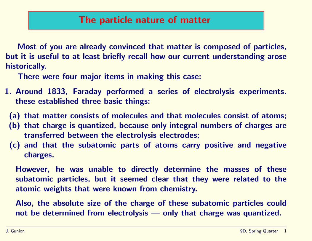
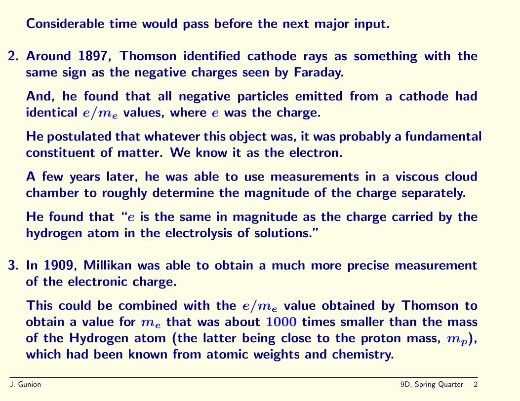
The apparatus and schematic are shown below. We consider a ~B fieldpointing into the page and a ~E field in the plane of the page. Whenpresent, these produce forces ~FE = −e~E (upwards) and ~FB = −e(~v× ~B)(downwards) on the e−.


Fig. 4−5, p. 111

Click to add title

Fig. 4−6, p. 111


First, turn on just the ~E field. Initially, upon entering from the left, onlyvx is non-zero, but upon exiting vy = ayt, where

ay =F

me

=eE

me

=V e

medand t =

l

vx. (1)

This gives

vy =V le

mevxd, tan θ =

vy

vx=V l

v2xd

(e

me

). (2)

So a measurement of θ gives us a value for eme

provided we can determinevx. Thomson determined vx, which remained the same if he kept hisaccelerating anodes at the same voltages, etc., by adding to ~E the ~Bfield. The forces exactly balance (and the e− is undeflected) when (forany q, including q = −e)

qE = qvxB , ⇒ vx =E

B=

V

dB. (3)


Thus, using the ~B that gives exact balance, we get

e

me

=v2xd tan θ

V l=V tan θ

B2ld. (4)

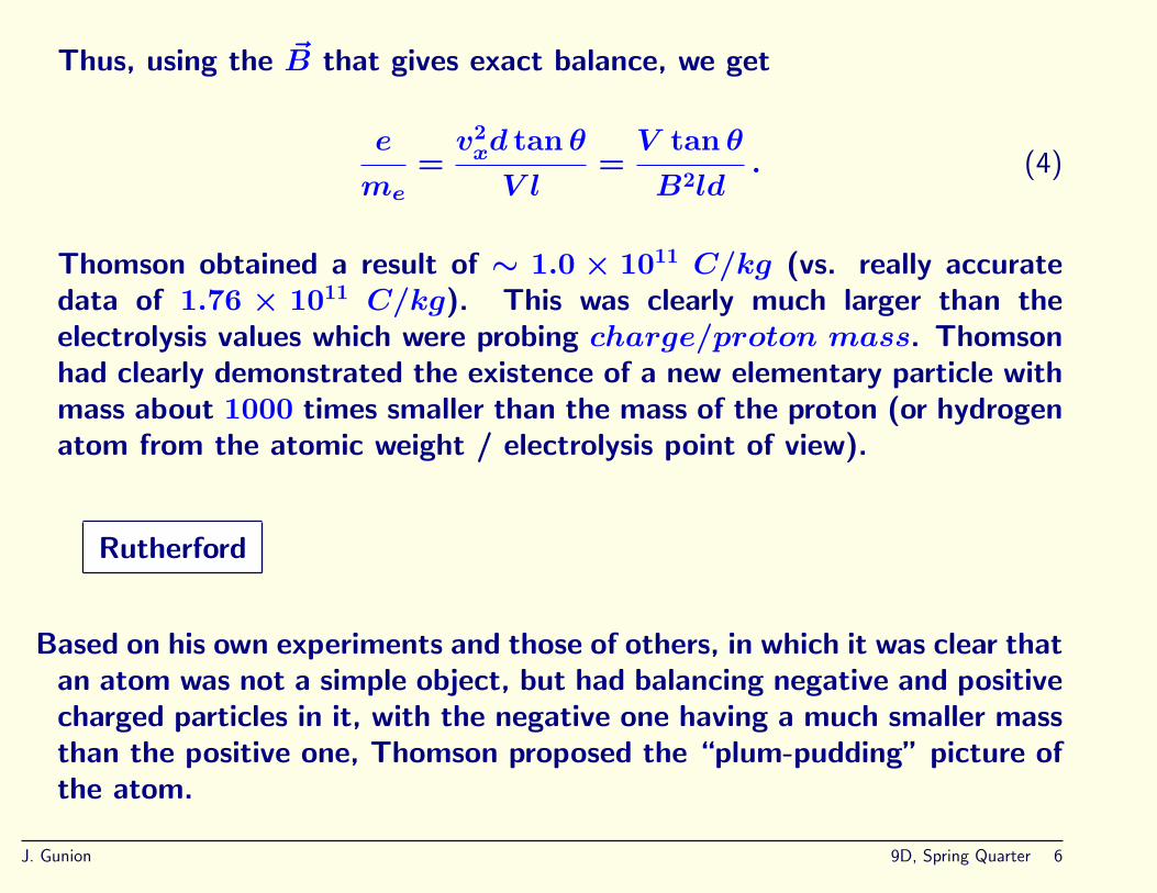
Thomson obtained a result of ∼ 1.0 × 1011 C/kg (vs. really accuratedata of 1.76 × 1011 C/kg). This was clearly much larger than theelectrolysis values which were probing charge/proton mass. Thomsonhad clearly demonstrated the existence of a new elementary particle withmass about 1000 times smaller than the mass of the proton (or hydrogenatom from the atomic weight / electrolysis point of view).

Rutherford

Based on his own experiments and those of others, in which it was clear thatan atom was not a simple object, but had balancing negative and positivecharged particles in it, with the negative one having a much smaller massthan the positive one, Thomson proposed the “plum-pudding” picture ofthe atom.


The atom was visualized as a homogeneous sphere of uniformly distributedmass and positive charge in which were embedded, like rasins in a plumpudding, negatively charged electrons, which just balanced the positivecharge to make the atom electrically neutral.

Of course, this picture failed to explain the rich line spectra that peoplewere finding for excited atoms, in particular even the simplest Hydrogenatom.

Rutherford and collaborators had noticed that a beam of α particles(i.e. Helium ions, 2p2n) broadened upon passing through a metal foil,indicating that the foil was quite easily penetrated and yet at the sametime caused significant scattering. This was hard to explain in the puddingmodel where the positive charge was spread all over the pudding.

After experimentation from 1909 to 1913, to be described, Rutherfordconcluded that all the positive charge, and most of the mass, wasconcentrated in a central nucleus of the atom. In particular, thispicture was the only one that produced events in which the α particlewas scattered at a very big angle, occassionally even backwards. Theexperimental apparatus and schematic picture of what is going on isdepicted on the following page.


Fig. 4−10, p. 120

Fig. 4−11, p. 121


In order to account for the occassional large angle, including backwards,deflections, Rutherford pictured the atom as having a central chargednuclear core and employed nothing more than Coulomb’s force law

F = k(2e)(Ze)

r2(5)

(where α has charge 2e in magnitude, the nucleus has charge Ze inmagnitude, and k is Coulomb’s constant). He predicted the followingresult for scattering:

∆n =k2Z2e4NnA

4R2(12mαv2

α)2 sin4(φ/2)

, (6)

where R and φ appear in the figure, N is the number of nuclei per unitarea of the foil (and is thus proportional to the foil thickness), n is thetotal number of α particles incident on the target per unit time, ∆n isthe number of α particles entering the detector per unit time at an angleφ, and A is the area of the detector. The velocity vα is determined fromthe accelerating potential difference between the α emitter and the goldfoil (or other) target: Kα = 1

2mαv2α = (2e)V (non-relativistic ok here,

and use charge of α = 2e).


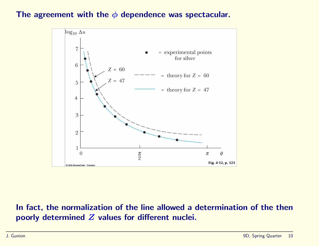
The agreement with the φ dependence was spectacular.

Fig. 4−12, p. 123

In fact, the normalization of the line allowed a determination of the thenpoorly determined Z values for different nuclei.


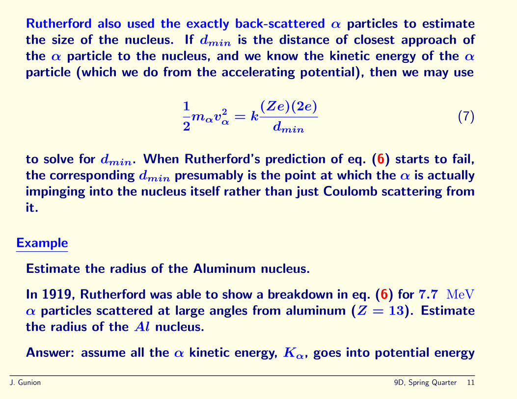
Rutherford also used the exactly back-scattered α particles to estimatethe size of the nucleus. If dmin is the distance of closest approach ofthe α particle to the nucleus, and we know the kinetic energy of the αparticle (which we do from the accelerating potential), then we may use

1

2mαv

2α = k

(Ze)(2e)

dmin(7)

to solve for dmin. When Rutherford’s prediction of eq. (6) starts to fail,the corresponding dmin presumably is the point at which the α is actuallyimpinging into the nucleus itself rather than just Coulomb scattering fromit.

Example

Estimate the radius of the Aluminum nucleus.

In 1919, Rutherford was able to show a breakdown in eq. (6) for 7.7 MeVα particles scattered at large angles from aluminum (Z = 13). Estimatethe radius of the Al nucleus.

Answer: assume all the α kinetic energy, Kα, goes into potential energy


at dmin. Then,

dmin = k2Ze2

Kα

= (8.99 × 109 N ·m2/C2)2(13)(1.6 × 10−10 C)2

(7.7 × 106 eV )(1.60 × 10−19 J/eV )= 4.9 × 10−15 m. (8)

Spectral Lines and Balmer

As mentioned earlier, many spectral lines had been seen, coming from thesun, coming from excited atoms, and so forth. There was no explanationyet. ***Do spectral line demo.***

A particularly famous result was the one obtained by Balmer in 1885.He managed to “fit” the results of Angstrom’s measurements of thewavelengths of the spectral lines from excited Hydrogen. These aredisplayed on the next page.


Fig. 4−20, p. 129

Balmer noted that the line wavelengths took the form:

λ(cm) = C2

(n2

n2 − 22

), n = 3, 4, 5, . . . (9)

where C2 = 3645.6 × 10−8 cm, a constant called the convergence limit


to which one tends as n → ∞. He further speculated that there wouldbe found other spectral line series of Hydrogen that would be fit by thegeneral form (equivalent for nf = 2 to the previous form)

1

λ= R

(1

n2f

−1

n2i

)(10)

where ni > nf and R = 1.0973732 × 107 m−1 is the Rydberg constantand is the same for all the different Hydrogen series lines. These seriescame to be named after the experimentalists that were first to see them:Balmer: nf = 2 (visible and near UV); Lyman: nf = 1 (more UV andharder to see); followed by Paschen, Brackett and Pfund (nf = 3, 4, 5)in the IR.

The groundwork was now in place for

Bohr

To understand how revolutionary Bohr’s ideas were, consider the conundrumthat the atomic physics people found themselves in. The picture of a


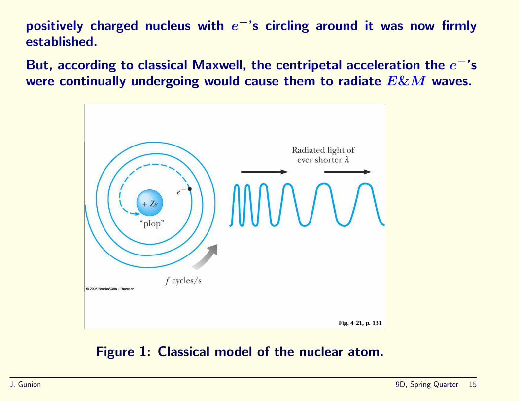
positively charged nucleus with e−’s circling around it was now firmlyestablished.

But, according to classical Maxwell, the centripetal acceleration the e−’swere continually undergoing would cause them to radiate E&M waves.

Fig. 4−21, p. 131

Figure 1: Classical model of the nuclear atom.


Classical theory would then imply that as the e−’s lose energy they wouldmove closer to the nucleus. Further, the spectrum of radiation from thiscontinuous process would change continuously, and one should not seesharp spectral lines.

In fact, as the e− gets closer to the nucleus it is moving faster andfaster in a stronger and stronger Coulumb field and the frequency of theradiation would get higher and higher.

Of course, we would not be around to see all this in any case.

Bohr followed the lead of Planck and Einstein by assuming that if lightwas quantized then why shouldn’t atomic electronic orbits be quantizedin some way. Then, spectral lines could arise when an electron jumpedfrom one such electronic orbit to another orbit (of lower energy) byemitting a photon of definite frequency given by ∆E = hf .

Armed with the picture of the atom just developed by Rutherford, in1913 Bohr published a 3-part paper in which he postulated that electronsin atoms are confined to stable, nonradiating energy levels and orbitsknown as stationary states.


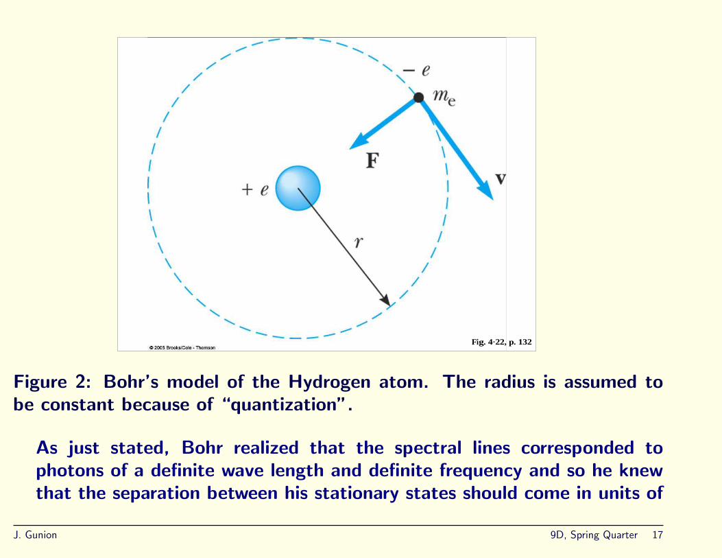
Fig. 4−22, p. 132

Figure 2: Bohr’s model of the Hydrogen atom. The radius is assumed tobe constant because of “quantization”.

As just stated, Bohr realized that the spectral lines corresponded tophotons of a definite wave length and definite frequency and so he knewthat the separation between his stationary states should come in units of


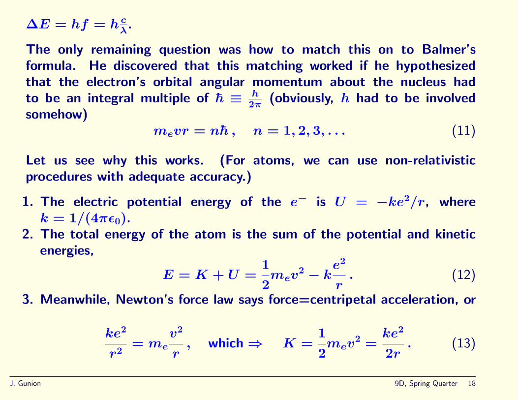
∆E = hf = hcλ.

The only remaining question was how to match this on to Balmer’sformula. He discovered that this matching worked if he hypothesizedthat the electron’s orbital angular momentum about the nucleus hadto be an integral multiple of h ≡ h

2π (obviously, h had to be involvedsomehow)

mevr = nh , n = 1, 2, 3, . . . (11)

Let us see why this works. (For atoms, we can use non-relativisticprocedures with adequate accuracy.)

1. The electric potential energy of the e− is U = −ke2/r, wherek = 1/(4πε0).

2. The total energy of the atom is the sum of the potential and kineticenergies,

E = K + U =1

2mev

2 − ke2

r. (12)

3. Meanwhile, Newton’s force law says force=centripetal acceleration, or

ke2

r2= me

v2

r, which ⇒ K =

1

2mev

2 =ke2

2r. (13)


4. Putting this result into the equation for E, eq. (12), gives

E = −ke2

2r. (14)

5. Next, we solve for v in terms of n and r using the equations above,

mevr = nh and 12mev

2 = ke2

2r , to obtain

rn =n2h2

meke2, n = 1, 2, 3, . . . (15)

r1 is often denoted by a0, and is called the Bohr radius,

a0 =h2

meke2= 0.0529 nm . (16)

6. Finally, substitute the form of rn into the equation for E just above,i.e. eq. (14), to obtain

En = −ke2

2a0

(1

n2

)= −

13.6

n2eV . (17)


The values n are called the quantum numbers characterizing differentstates.

The lowest state E1 = −13.6 eV is called the ground state.

The n = 2 state is the 1st excited state and has energy E2 = −3.4 eV,and so forth.

At this point, we can explain the Balmer formula.

1. A spectral photon is emitted when the atom drops from a state witha high n = ni to a state with more negative energy i.e. with smallern = nf .

2. The different series are obtained using nf = 1, nf = 2, . . . for thefinal lower-n state.

3. In other words, we have

1

λ=f

c=Ei − Ef

hc=

ke2

2a0h

(1

n2f

−1

n2i

). (18)

One finds that ke2/(2a0h) = R, the Rydberg constant and one gets atheoretical post-diction of the Balmer formula.


This is depicted in Fig. 3.

Fig. 4−24, p. 134

Figure 3: Bohr’s explanation of the various Hydrogen spectral series.

An Example

Suppose the stellar atmosphere has a temperature of order T =79, 000K. (a) Is it reasonable to expect that a lot of the Hydrogen atoms


will be excited to the first excited state? (b) What is the wavelengthof the light emitted when these excited atoms decay back to the n = 1ground state level?

First, we compute the average thermal energy per atom:

3

2kBT = (1.5)(8.62 × 10−5 eV/K)(79000) = 10.2 eV . (19)

This, we must compare to the energy of excitation,

E2 − E1 = −3.4 eV − (−13.6 eV ) = 10.2 eV . (20)

Since these are comparable, we expect substantial excitation.

The wavelength could either be obtained from the Balmer formula or wecan return to Bohr’s basic model according to which

hf = E2 − E1 ⇒

λ =hc

E2 − E1=

(4.136 × 10−15 eV · s)(3 × 108 m/s)

10.2 eV= 1.22 × 10−7 m = 122 nm , (21)


well into the ultraviolet.

Bohr immediately realized that all of this could be extended to ionsobtained from an element with a given nuclear charge Z by removing allbut one of the e−’s.

Such an ion has a single e− orbiting about a nuclear charge of +Ze.Proceeding as above, but using the higher nuclear charge, one obtains

rn = n2a0

Z, implying En = −

ke2

2a0

(Z2

n2

), n = 1, 2, 3, . . . (22)

When applied to He+, several previously unexplained spectral lines inradiation from the sun were explained.

An Example

Pickering, in 1896, observed unexpected spectral lines in the light fromξ-Puppis, a star.

He found that these lines fit the spectral formula

1

λ= R

(1

(nf/2)2−

1

(ni/2)2

), (23)


where R is the Rydberg constant. We can easily check that these linesare simply those associated with He+ as follows.

Since He+ has nuclear charge of Z = 2, we have energy levels given by

En =ke2

2a0

(4

n2

). (24)

Using hf = Ei − Ef , we then have

1

λ=

f

c=Ei − Ef

hc

=ke2

2a0hc

(4

n2i

−4

n2f

)=

ke2

2a0hc

(1

(ni/2)2−

1

(nf/2)2

)(25)

where ke2/(2a0hc) = R is precisely the Rydberg constant.


An interesting question from the class

During the lecture on this material, an interesting question was asked.This concerned why we don’t see atoms absorbing starlight. Well, infact we do. As we discussed, one should visualize a distant star sendinglight towards the earth, with some dust or gas cloud (for example) inbetween the star and the earth. If the cloud mainly contains Hydrogen,for example, then starlight with the right frequency to excite a Hydrogenatom from a low energy (e.g. ground) state to a higher state will oftenget absorbed and not make it through the cloud. We get what are calledabsorption spectra (that can be used to help determine the red-shift ofthe star relative to the cloud and of the cloud relative to us).

The energy of the star radiation can even be sufficient to completelyionize the Hydrogen atom if the cloud is close to the star or the star isof a particularly energetic type.

A second question was why one doesn’t get radiation, coming from theexcited atom when it falls back to its ground state, that fills in theabsorption line.

In fact, there is such radiation, but it goes in all directions (not justtowards the earth) and so the amount headed towards earth is greatly


diminished.

An important dimensionless ratio

It turns out to be interesting to consider the ratio

vn=1

c=

1

c

h

mr1from mvr = nh

=1

c

ke2

hfrom r1 = h2

meke2

=ke2

hc≡ α =

1

137. (26)

Note how small v1/c is. The non-relativistic approximation employed byBohr was ok.

The quantitiy α is sometimes called the fine structure constant. It is avery useful characterization of the strength of the E&M force. Otherforces, such as the strong and weak forces that we will learn more aboutlate in the quarter, have different strengths.

Such dimensionless ratios constructed using known physical constants(here, h, c, k and e) are typically of deep theoretical significance. Toconstruct α, we needed the new fundamental constant h.


The correspondence principle

One justification given by Bohr for his angular momentum quantizationcondition is that it is required if we demand a correspondence principleaccording to which

limn→∞

[quantum physics] = [classical physics] (27)

where n is a typical quantum number of the system such that large ncorresponds to a limit in which one should approach a classical type ofsituation, such as long wavelengths.

We will not go into the details of this in class.

Franck and Hertz

Of course, the critical assumption made by Bohr in his explanation of thespectral lines was that an electron could be in a higher n state and thatwhen it “fell” down to a lower state it emitted a single photon.

A direct verification that the photon energies corresponded to theseparation between energy levels of the electron of the atom was needed.


Franck and Hertz provided an explicit experimental demonstration thatthis was indeed the case.

They sealed some Mercury Hg inside a tube and accelerated e−’s throughthe tube using a voltage V . These e−’s then collide with the Hg atomsinside the tube, possibly giving energy to them.

Fig. 4−27, p. 141

Figure 4: The Franck-Hertz apparatus.

For small V , these collisions were elastic and the e−’s retained most of


their kinetic energy (very little is taken by the much more massive Hgatoms in an average collision). Even after many collisions, the e− arrivesat the accleration grid with energy of about eV .

Following this acceleration, their apparatus had a retarding voltage gapbetween the accelerating grid and the following collector plate of about1.5 V . Thus, some e−’s will be collected if V > 1.5 V .

Fig. 4−28, p. 142

Figure 5: The Franck-Hertz current as a function of accelerating voltage V .

As V is increased, more and more e−’s make it to the collector until


the energy eV that the electrons have acquired matches the energydifference between two atomic energy levels. At this point, the collisionbetween some of the accelerated e−’s and the Hg can be inelastic —the Hg atom absorbs the K = eV energy of the e− when one of its ownelectrons is excited to a higher n level.. There is a sudden dip in thecurrent reaching the collector.

When V is increased further, more and more electrons reach the collectoruntil once again the current suddenly dips. What is happening is that Vis large enough for the accelerated e−’s to have two inelastic collisionswith two subsequent Hg atoms.

The separation between the dips was found to be ∆V ∼ 4.9 V . Theyinterpreted e∆V as being the energy difference between the ground stateof low n for one of the Mercury orbiting electrons and the next excitedstate of this same electron.

How could they check this? Well, if they really had excited the Hg atomicelectron to a higher level, it should emit a photon of the correspondingfrequency when this electron fell back down to its original lower level.


The expected wave length of the photon was therefore given by

e∆V = ∆E = hf =hc

λ, ⇒ λ =

hc

∆E=

1240 eV · nm4.9 eV

= 253 nm .

(28)This is the precise wavelength they observed. In 1925, they were awardedthe Nobel prize for this confirmation of Bohr’s theory.

Connection of Bohr quantization to the wave nature of matter

The next big question was why should angular momentum be quantizedin the manner proposed by Bohr?

What turns out to be the fundamental idea was that developed by deBroglie in 1925.

He speculated that if light, a wave phenomenon originally, also had aparticle-like nature, then why not the reverse?

He also was looking for a way to explain the integers and quantizationthat emerged in Bohr’s atomic theory, which concerned electrons circlinga nucleus. The only way that integers had cropped up in the past was


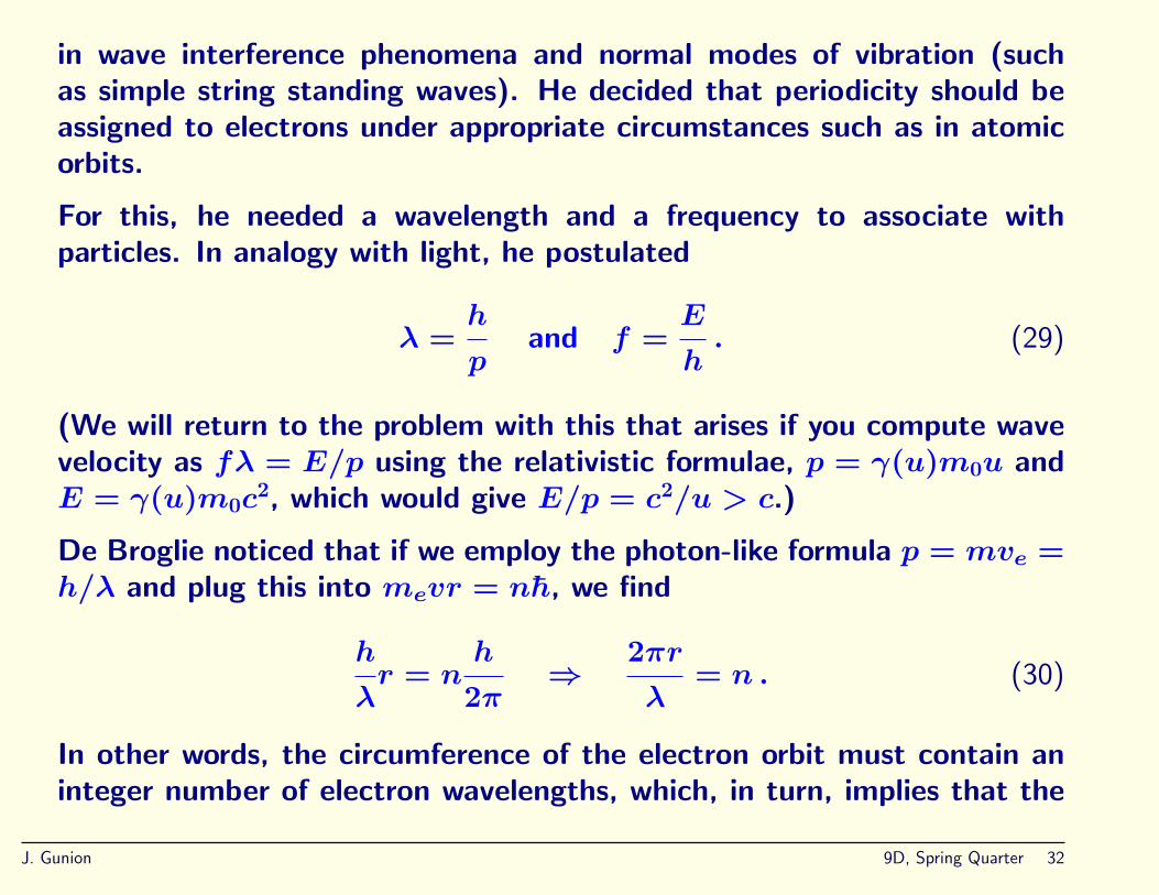
in wave interference phenomena and normal modes of vibration (suchas simple string standing waves). He decided that periodicity should beassigned to electrons under appropriate circumstances such as in atomicorbits.

For this, he needed a wavelength and a frequency to associate withparticles. In analogy with light, he postulated

λ =h

pand f =

E

h. (29)

(We will return to the problem with this that arises if you compute wavevelocity as fλ = E/p using the relativistic formulae, p = γ(u)m0u andE = γ(u)m0c

2, which would give E/p = c2/u > c.)

De Broglie noticed that if we employ the photon-like formula p = mve =h/λ and plug this into mevr = nh, we find

h

λr = n

h

2π⇒

2πr

λ= n . (30)

In other words, the circumference of the electron orbit must contain aninteger number of electron wavelengths, which, in turn, implies that the


electron wave pattern will repeat by matching onto itself after goingaround a full orbit. In other words, an electron orbit should correspondto a standing, self-reinforcing wave pattern, much like a plucked guitarstring.

Fig. 5−2, p. 153

Figure 6: De Broglie’s explanation of Bohr quantization for the case ofn = 3, showing self-reinforcing standing wave pattern for an e− around thenucleus with three wave lengths fitting into 2πr circumference.

We will soon turn to more discussion and eventual direct confirmation of


the association of a wavelength with a massive particle using λ = h/p.

In the end, we will see that this standing wave pattern and the whole Bohrpicture is not an accurate point of view. However, it was very critical todeveloping the correct view that we now call Quantum Mechanics.


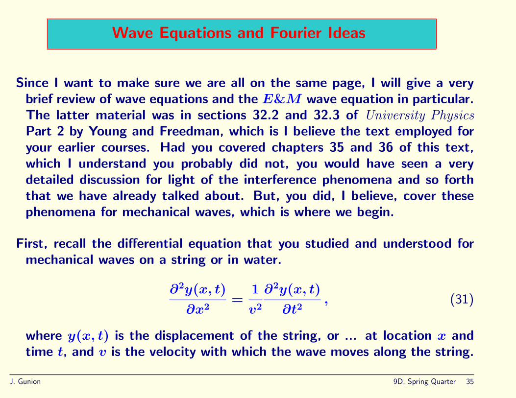
Wave Equations and Fourier Ideas

Since I want to make sure we are all on the same page, I will give a verybrief review of wave equations and the E&M wave equation in particular.The latter material was in sections 32.2 and 32.3 of University PhysicsPart 2 by Young and Freedman, which is I believe the text employed foryour earlier courses. Had you covered chapters 35 and 36 of this text,which I understand you probably did not, you would have seen a verydetailed discussion for light of the interference phenomena and so forththat we have already talked about. But, you did, I believe, cover thesephenomena for mechanical waves, which is where we begin.

First, recall the differential equation that you studied and understood formechanical waves on a string or in water.

∂2y(x, t)

∂x2=

1

v2

∂2y(x, t)

∂t2, (31)

where y(x, t) is the displacement of the string, or ... at location x andtime t, and v is the velocity with which the wave moves along the string.


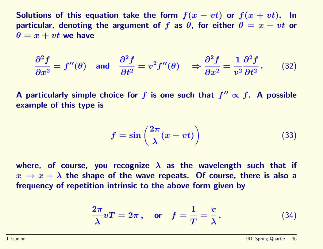
Solutions of this equation take the form f(x − vt) or f(x + vt). Inparticular, denoting the argument of f as θ, for either θ = x − vt orθ = x+ vt we have

∂2f

∂x2= f ′′(θ) and

∂2f

∂t2= v2f ′′(θ) ⇒

∂2f

∂x2=

1

v2

∂2f

∂t2. (32)

A particularly simple choice for f is one such that f ′′ ∝ f . A possibleexample of this type is

f = sin(

2π

λ(x− vt)

)(33)

where, of course, you recognize λ as the wavelength such that ifx → x + λ the shape of the wave repeats. Of course, there is also afrequency of repetition intrinsic to the above form given by

2π

λvT = 2π , or f =

1

T=v

λ. (34)


Often, it is more convenient to write

2π

λ(x− vt) ≡ kx− ωt , (35)

where k ≡ 2π/λ and you can check that ω = 2πf .

We should also recall that one can superimpose different solutions of thewave equation and still get a solution. For example,

ei(kx−ωt) and e−i(kx−ωt) (36)

are both also solutions to the wave equation and the earlier sin form canbe written as (using eib = cos b+ i sin b)

sin(kx− ωt) =1

2i

[ei(kx−ωt) − e−i(kx−ωt)

]. (37)

Of course, in the case of a real observable thing like the stringdisplacement, when we superimpose these complex exponentials, weshould always do so in such a way that the superposition has a real value.But, it is nonetheless convenient to use the complex exponentials. In


fact, as we shall see, matter waves are intrinsically complex and can beso because the waves have no direct physical manifestation. It is onlytheir |amplitude|2 that can be interpreted as probability.

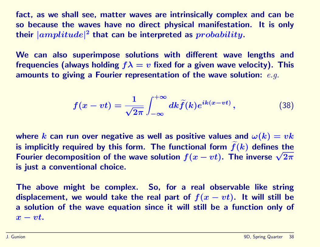
We can also superimpose solutions with different wave lengths andfrequencies (always holding fλ = v fixed for a given wave velocity). Thisamounts to giving a Fourier representation of the wave solution: e.g.

f(x− vt) =1

√2π

∫ +∞

−∞dkf(k)eik(x−vt) , (38)

where k can run over negative as well as positive values and ω(k) = vk

is implicitly required by this form. The functional form f(k) defines theFourier decomposition of the wave solution f(x− vt). The inverse

√2π

is just a conventional choice.

The above might be complex. So, for a real observable like stringdisplacement, we would take the real part of f(x − vt). It will still bea solution of the wave equation since it will still be a function only ofx− vt.


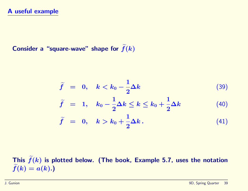
A useful example

Consider a “square-wave” shape for f(k)

f = 0, k < k0 −1

2∆k (39)

f = 1, k0 −1

2∆k ≤ k ≤ k0 +

1

2∆k (40)

f = 0, k > k0 +1

2∆k . (41)

This f(k) is plotted below. (The book, Example 5.7, uses the notationf(k) = a(k).)


Fig. 5−23, p. 172

Figure 7: Input k-space function.

The resulting analytic form for f(x− vt) at t = 0 (derived a bit later) is

f(x) =∆k

√2π

sin(∆k · x/2)

(∆k · x/2)eik0x , (42)

the real part of which is plotted in the figure.


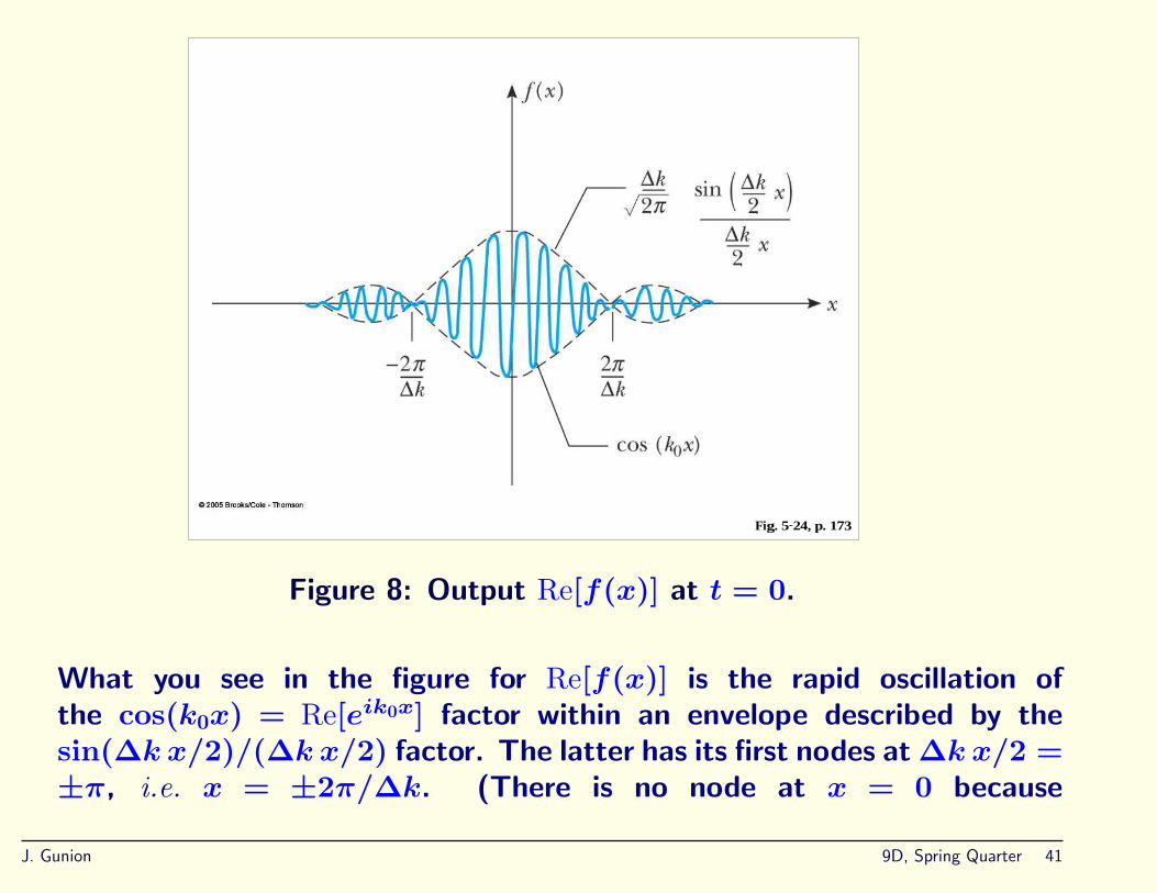
Fig. 5−24, p. 173

Figure 8: Output Re[f(x)] at t = 0.

What you see in the figure for Re[f(x)] is the rapid oscillation ofthe cos(k0x) = Re[eik0x] factor within an envelope described by thesin(∆k x/2)/(∆k x/2) factor. The latter has its first nodes at ∆k x/2 =±π, i.e. x = ±2π/∆k. (There is no node at x = 0 because


limx→0 sinx/x = 1.) The full width between the two nodes is thus∆x = 4π/∆k.

What we wish to particularly point out is the relationship between thewidth of the input bump in k space to the width of the output wave formin x space. We have

∆x∆k = 4π . (43)

The smallest value for this product occurs if a Gaussian form (f(k) ∝e−1

2(k−k0)2/(δk)2) is employed. The output then has a similar Gaussian

shape in x (f(x) ∝ e−12(x−x))

2/(δx)2), with δx = 1/δk, or δxδk = 1.With a certain “formal” defintion of ∆x and ∆k that we will come to,∆x = δx/

√2 and ∆k = δk/

√2, and we obtain

∆x∆k =1

2. (44)

Thus, for any possible form of f(k), we have

∆x∆k ≥1

2. (45)


The Heisenberg Uncertainty Relation for Photon Waves

So what? What is the physical impact? First, as we shall remind ourselvesin more detail in a moment. Light obeys the same kind of wave equationjust considered, with v = c.

Next, let us input the light wave / photon relation that

k =2π

λ=

2πp

h=p

h, (46)

eq. (45) can be rewritten as

∆x∆p ≥h

2. (47)

This is the famous Heisenberg uncertainty principle that was first proposedfor matter, and only later was it realized that it was already present inthe description of light waves as photon packets with p = h/λ.

We will return to a thorough discussion of the implications of this kind ofuncertainty principle. However, you should at this point take note of the


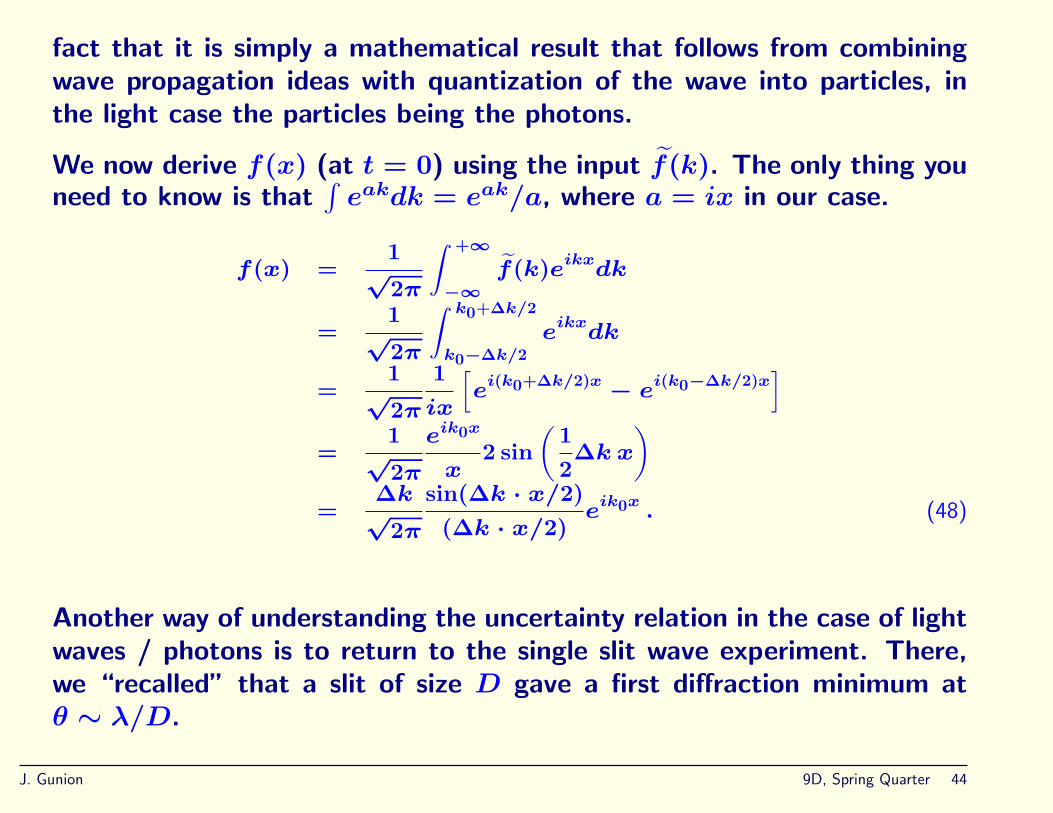
fact that it is simply a mathematical result that follows from combiningwave propagation ideas with quantization of the wave into particles, inthe light case the particles being the photons.

We now derive f(x) (at t = 0) using the input f(k). The only thing youneed to know is that

∫eakdk = eak/a, where a = ix in our case.

f(x) =1

√2π

∫ +∞

−∞f(k)eikxdk

=1

√2π

∫ k0+∆k/2

k0−∆k/2eikxdk

=1

√2π

1ix

[ei(k0+∆k/2)x − e

i(k0−∆k/2)x]

=1

√2π

eik0x

x2 sin

(12∆k x

)=

∆k√

2π

sin(∆k · x/2)(∆k · x/2)

eik0x . (48)

Another way of understanding the uncertainty relation in the case of lightwaves / photons is to return to the single slit wave experiment. There,we “recalled” that a slit of size D gave a first diffraction minimum atθ ∼ λ/D.


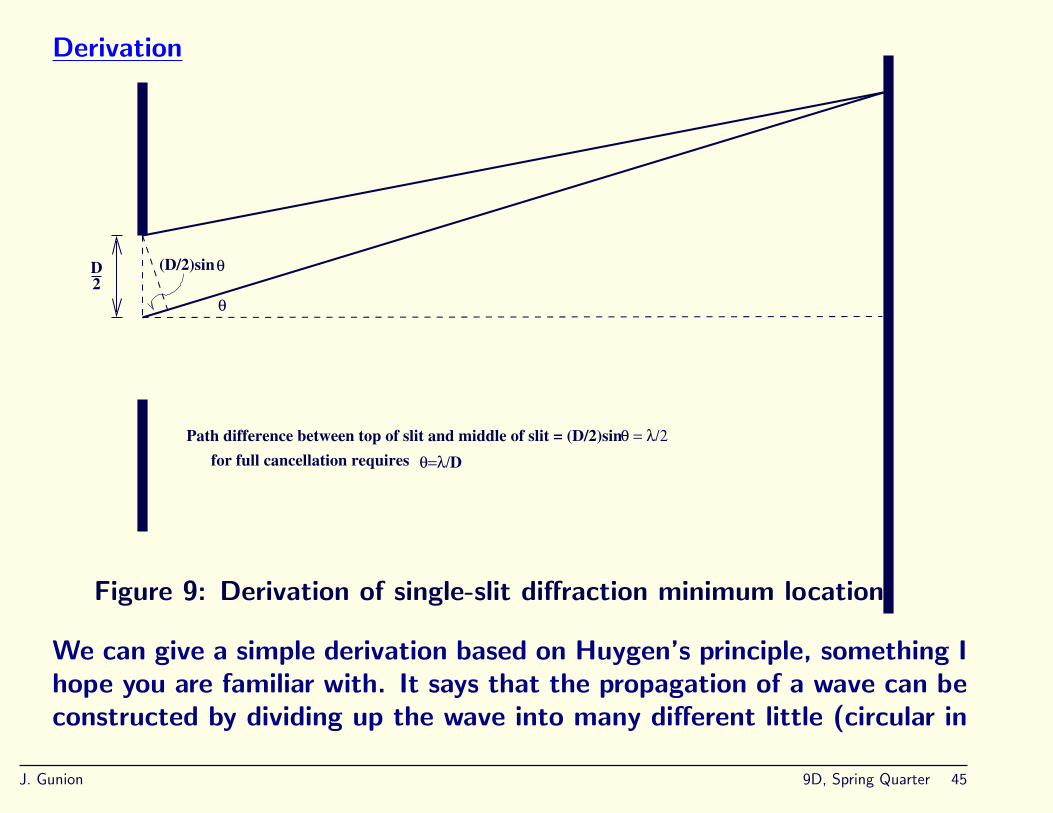
Derivation

D2

θ

(D/2)sinθ

for full cancellation requires θ=λ/DPath difference between top of slit and middle of slit = (D/2)sin θ = λ/2

Figure 9: Derivation of single-slit diffraction minimum location.

We can give a simple derivation based on Huygen’s principle, something Ihope you are familiar with. It says that the propagation of a wave can beconstructed by dividing up the wave into many different little (circular in


a planar configuration) wavelets emanating from any well defined surface(curve in a planar configuration).

Using Huygen’s principle, consider a wavelet emanating from the top ofthe slit and one from the midpoint of the slit. The diagram shows thatthese two wavelets will be precisely 1/2 wavelength out of phase (i.e.they will cancel) when sin θ ∼ θ = λ/D. The same will apply to awavelet emanating from ε below top and ε below the midpoint, and soforth. Thus, θ ∼ λ/D is the condition for a minimum in the diffractionpattern.

Demonstration

Take a red laser, λ ∼ 650 nm = 0.65 × 10−6 m. Take a slit oforder D = 0.2 mm = 2 × 10−4 m. The first minimum will be atθ ∼ 0.0032. Place a screen about l = 10 m away and the distancebetween the two first minima on either side of the maximum should beabout d = 2lθ ∼ 0.065 m = 6.5 cm.

Implications for photon momenta

For the photon to have travelled there, it must pick up a momentumpy perpendicular to the initial (upwards) momentum of px ∼ p = h/λ.


Thus, we have

θ ∼py

px∼pyλ

h⇒ py ∼

θ h

λ∼λ

D

h

λ∼h

D(49)

from which we find (can’t expect to get 2π type factors right here)

∆py∆y ∼ pyD ∼h

DD ∼ h . (50)

Once again, the uncertainty relationship emerges. Here, we have triedto confine the E&M wave to a location of size D in the y direction asit propagates to the right in the x direction, and, in so doing, we havegenerated a substantial uncertainty in py. The more we try to define thewave location in a certain direction, the greater the uncertainty in themomentum in that same direction.


Electromagnetic Waves

Let me now give a brief review of the E&M wave equation. Had I knownthat this was only given very brief attention in your previous course, Iwould have surely begun this quarter’s lectures with the following review.

One starts with the two Maxwell equations:∮C

~E · d~l = −d

dt

∫S

~B · n dA (51)∮C

~B · d~l = µ0ε0d

dt

∫S

~E · n dA (52)

where the latter assumes no source current I, as appropriate forpropagation in a vacuum. The vector n represents a unit vector normalto the surface S at any given point. The closed loop C runs along theboundary of the surface S, and the orientation of n relative to C is givenby the right-hand rule.

In principle, you have read the material in University Physics Section 32to learn that these reduce (for a wave traveling in the x direction with ~E


pointing in the y direction and ~B pointing in the z direction) to

∂Ey

∂x= −

∂Bz

∂t(53)

∂Bz

∂x= −µ0ε0

∂Ey

∂t(54)

I give a brief derivation of the first equation. We apply eq. (51) to thecase of ~E = yEy and ~B = zBz. The equation says that a time varyingBz (using n = z and very small size dx by dy loop in the x, y plane) cangenerate an ~E field that circulates around the small loop. Applying thisto the ~E = yEy case, we find that Ey must vary with x. In short, thetime varying Bz field is generating a spatial variation of Ey as a functionof x. Of course, Ey will end up with time dependence that matches thatof the time derivative of Bz. A figure showing how this application worksis below.


n

B_z(x)

x

y

z

dx

dy

E_y(x+dx)

E_y(x)

E loop integral = E_y(x+dx)dy − E_y(x) dy = (dE_y(x)/dx)dxdy

B surface integral = B_z(x) dx dy

Figure 10: Set up for deriving eq. (53).

The 2nd of the integral-form Maxwell equations (applied with n = y anda very small loop in the x, z plane of size dx by dz) implies that a spatialvariation of Bz as a function of x will be generated by a time variation


of Ey. A set up analogous to that depicted in Fig. 10 would give youeq. (54).

Equivalently, you may have seen the two integral equations rewrittenusing the famous general theorem, called Stoke’s theorem, which states:∮

C

~F · d~l =∫S

(~∇ × ~F ) · n dA (55)

where ~F is any arbitrary vector “field” and ~∇ × ~F denotes the “curl” of~F . The two important components of the definition of the curl are

(~∇ × ~F )z =∂Fy

∂x−∂Fx

∂y(56)

(~∇ × ~F )y =∂Fx

∂z−∂Fz

∂x; (57)

these will be needed in the differential forms of eqs. (51) and (52),respectively.

Using this theorem in eqs. (58) and (59) and the fact that the surfaceS, and its normal n, can be thought of as being arbitrary, the integrands


must be equal so that eqs. (51) and (52) imply

~∇ × ~E = −∂ ~B

∂t(58)

~∇ × ~B = µ0ε0∂ ~E

∂t, (59)

respectively. We now assume, as above, that ~B = zBz only and~E = yEy only. In this case, we are interested in the z component ofeq. (58) and the y component of eq. (59). We then employ the curldefintions of eqs. (56) and (57) to obtain

(~∇ × ~E)z =∂Ey

∂x, (~∇ × ~B)y = −

∂Bz

∂x. (60)

Substituting the above into eqs. (58) and (59), respectively, we geteqs. (53) and (54), repeated below.

∂Ey

∂x= −

∂Bz

∂t(61)

−∂Bz

∂x= µ0ε0

∂Ey

∂t(62)


Let us now consider the equation that can be derived from eqs. (53) and

(54). Take ∂∂x

eq. (53) ⇒ ∂2Ey∂x2 = − ∂

∂t∂Bz∂x

and substitute for ∂Bz∂x

using

eq. (54), which states ∂Bz∂x

= −µ0ε0∂Ey∂t

to obtain:

∂2Ey

∂x2= µ0ε0

∂2Ey

∂t2. (63)

This matches the mechanical wave equation provided the velocity isv2 ≡ c2 = 1

µ0ε0. Following a similar procedure we also find

∂2Bz

∂x2= µ0ε0

∂2Bz

∂t2. (64)

Thus, the E and B oscillations are continually feeding one anotherthrough Maxwell’s laws and as a result the wave propagates in the xdirection.

If we employ a form

Ey = A sin(kx− ωt) , (65)


then we can check that the associated form for Bz must be

Bz =1

cA sin(kx− ωt) , (66)

by employing either eq. (53) or eq. (54). For example, eq. (54) states

that ∂Bz∂x

= − 1c2∂Ey∂t

. Substituting in the above forms we get

∂Bz

∂x=

1

cAk cos(kx− ωt)

−1

c2∂Ey

∂t= −

1

c2A(−ω) cos(kx− ωt)

=1

cAω

ccos(kx− ωt)

=1

cAk cos(kx− ωt) using ω/k = c . (67)

The fact that Ey and Bz are exactly “in phase” all the time, is one ofthe remarkable features of E&M radiation. But, it had to be true inorder for one to “feed” the other.


Energy carried by an E&M wave

It is also useful to remind ourselves about the amount of energy carriedby an E&M wave. You need to remember that the energy density storedin the ~E and ~B fields is given by

uE =1

2ε0 ~E · ~E , uB =

1

2

~B · ~Bµ0

, (68)

respectively. As we have seen above, for the travelling wave, | ~B| = |~E|/c.So, u = uE + uB can be written in a variety of forms:

u =1

2ε0|~E|2 +

1

2

| ~B|2

µ0

= ε0|~E|2

=| ~B|2

µ0

=√ε0

µ0|~E|| ~B| . (69)


And, we should also remember that for the E&M wave, travelling withvelocity c, the amount of energy transported through a surface areaperpendicular to the wave’s direction of travel (e.g. a surface in they, z plane for travel in the x direction) is simply S = cu, which hasthe correct dimensions since c = m/s while u = energy/m3 so thatS = energy/m2/s.

An Example

Suppose the maximum |~E| value for a traveling sinusoidal wave, moving inthe x direction is Emax = |~E| = 100 N/C and occurs at t = 0, x = 0.Give a value for the amount of energy impacting a screen perpendicularto the x axis per unit area per unit time at t = 0, x = (2/3) × λ.

Answer: Since the field is maximum at t = 0, x = 0, it is convenientto use the form Ey = Emax cos

(2πλ

(x− ct)). Substituting t = 0, x =

(2/3)λ gives Ey = Emax cos(4π/3) = −12Emax. From our earlier

equations, we have

S = cu = cε0E2y

= (3 × 108 m/s)(8.85 × 10−12 C2/N ·m2)(−1

2100 N/C)2


= 6.6375 J/(m2 · s) . (70)

Of course, as time passes, at this same location, the S value will oscillateup and down and so the average energy per unit area per unit time willbe Saverage = 1

2Smax = 12cε0E

2max. This is what we usually call the

intensity of the E&M wave, but we see that a more accurate namewould be average intensity.

We do not know how many photons this corresponds to (on average)until λ is specified. Also note that we could compute (at any instant)Bz using Bz = Ey/c.

Momentum Carried by an E&M wave

We have stated that the relation between the energy and the momentumcarried by an E&M wave is p = E/c, where in the continuous wavevision E is the same as S. p will then be so much momentum per unitarea per unit time.

To derive this relation between the energy and momentum carried byan E&M wave, is a bit of an exercise. I give it below in case you areinterested.


Consider a test charge Q (of unit area) on which the wave impinges. Thewave will start this test charge moving, to begin with in the y directionas a result of Fy = QEy. Once Q has some vy, the magnetic field ofthe wave will act on it to produce a force in the x direction

Fxx = Qvyy ×Bzz = xQvyBz . (71)

Since Fx = dpx/dt, we get momentum being fed to the charge at therate of (using Bz = Ey/c, as above)

dpx

dt= QvyBz = Qvy

Ey

c. (72)

Meanwhile, starting from vx = 0 (so that Fx is not doing any x directionwork yet) potential energy is being added to this charge, because it ismoving against the electric field, according to

∆U = QEy∆y , ⇒dU

dt= QEyvy . (73)

Substituting the result of solving this equation for vy into the previous


equation givesdpx

dt= Q

(dU/dt

QEy

)Ey

c=

1

c

dU

dt, (74)

implying that on a per second basis the amount of energy being suppliedby the E&M wave and the amount of x momentum being supplied bythe wave must be related by p = U/c. But, the amount of energy beingsupplied by the E&M wave (all this is per unit area per unit time, recall)is simply U = S. We have been denoting S by E, which, to repeat,for a wave is the amount of energy per unit are per unit time passinga certain perpendicular plane. And, of course, if both the momentumand the energy are being carried by photons, then the energy per photonmust be related to the momentum per photon by p = E/c.

Return to previous example

At t = 0, x = (2/3)λ, how much momentum is being transferred tothe screen per unit area per unit time, assuming that all the radiation isbeing absorbed?

Answer: Using E = S = cp, we compute

p =S

c=

6.6375J/(m2 · s)3 × 108 m/s

= (2.212× 10−8 kg ·m/s)/(m2 · s) . (75)


Hopefully, the demonstration of a little set of vanes inside a vacuumcontainer is something you have seen?

General Lesson

Thus, just as in the case of a wave on a string, the ~E and ~B fieldscontained in a light wave have real physical implications. ~E couldaccelerate a charged test particle and ~B could deflect a moving chargedtest particle.

A Lesson in Wave Amplitudes and Probabilities

We have seen that a single slit will have a minimum at sin θ = λ/Dcoming from the complete cancellation of various Huygen’s waveletamplitudes from different parts of the slit. At θ = 0, all the waveletsarrive in phase at the central point of the screen and simply add up togive you a maximum E field, call this maximum E0. E0 will have somewave-like form, of course, and so will oscillate up and down as time passesaccording to some form like

E0 = Emax sin(

2π

λ(xscreen − ct)

). (76)


There will be an instantaneous intensity I0 = cε0|E0|2 and the averageintensity will be 〈I0〉 = 1

2Imax0 = 1

2cε0|Emax|2.

One can also add up the wavelets for any other θ. I will not go throughthe derivation, but the result is

E = E0sin[πD(sin θ)/λ]

πD(sin θ)/λ, ⇒ I = I0

{sin[πD(sin θ)/λ]

πD(sin θ)/λ

}2

(77)

Now let us consider the case of D � λ. Then, since limx→0sinxx

= 1we have E = E0, independent of θ. That is, uniform intensity on thedetecting screen.

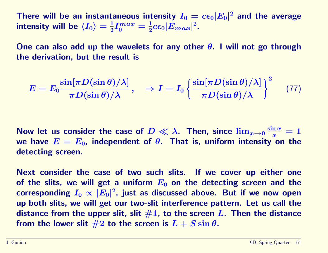
Next consider the case of two such slits. If we cover up either oneof the slits, we will get a uniform E0 on the detecting screen and thecorresponding I0 ∝ |E0|2, just as discussed above. But if we now openup both slits, we will get our two-slit interference pattern. Let us call thedistance from the upper slit, slit #1, to the screen L. Then the distancefrom the lower slit #2 to the screen is L+ S sin θ.


S

θ

S sin θ

θ

θ

Path difference between top slit and bottom slit = S sin

L

L + S sin θ

Figure 11: Two (narrow) slit interference.

From this picture, we obtain

E1+2 = E

1 + E2

= Emax

[sin

(2πλ

(L− ct))

+ sin(

2πλ

(L + S sin θ − ct))]

.

First, let us note that the two waves cancel when S sin θ = (n + 12)λ,


since the arguments of the sin’s would differ by π, i.e. one-half cycle.Thus, the two-slit pattern will have minima with zero intensity at suchangles. Correspondingly, the two-slit pattern maxima occur at S sin θ =nλ. At such angles, constructive addition of the two waves is perfect.

Of course, for general θ, L = xscreen/ cos θ, but this is not needed forthe above discussion.

Now, let us return to the question posed at the end of the last class, forwhich we focus on the case of θ = 0. Then,

E1+2 = 2Emax sin(

2π

λ(xscreen − ct)

), ⇒ I1+2 = 4cε0|E0|2

(78)implying that I1+2 = 4I0, where I0 is that from just one slit! Here, I0denotes the instantaneous intensity. For the average intensity, the sameapplies:

〈I1+2〉 = 4〈I0〉 = 4[1

2Imax0

]. (79)


What about matter waves?

In contrast, as I have said before, the matter waves that we shall cometo do not have any such direct physical interpretation.

Matter waves are sort of like putting the ~E and ~B together in the form

~F = ~E + ic ~B . (80)

If we take the absolute square of this ~F , we get

|~F |2 = (~E + ic ~B) · (~E − ic ~B) = |~E|2 + c2| ~B|2 (81)

which is indeed proportional to the intensity of the electromagnetic wave.We have learned that it is the intensity that tells us the probability offinding a photon at a certain point in space at a certain time.

For matter waves, the wave will usually be denoted by Ψ. Ψ can alwaysbe decomposed into its real and imaginary parts:

Ψ = Ψ1 + iΨ2 . (82)


For matter waves, Ψ1 and Ψ2 do not have any direct physical manifestationanalogous to the way in which ~E and ~B can impact a test charge. Thereis no test probe that one can employ. The only interpretation of Ψ isthat

Probability of finding particle ∝ |Ψ|2 = |Ψ1|2 + |Ψ2|2 . (83)

Ad hoc derivation of E&M wave equation

Before ending this “review”, let me note an amusing “derivation” of theE&M wave equation.

First, we note again that the wave equation for X being either Ey or Bztakes the form

∂2X

∂x2=

1

c2∂2X

∂t2. (84)

Suppose we write the energy momentum relationship for light in the form

p2 = E2

c2, multiply this times X and then make the replacements

E → ih∂

∂tand p →

h

i

∂

∂x. (85)


Then,

p2X =E2

c2X ⇒ −h2

[∂2X

∂x2=

1

c2∂2X

∂t2

], (86)

which contains our wave equation. A hand-waving motivation for theseidentifications is to note that for a wave solution of the type eik(x−ct)

(our general form for the case of v = c) that we were discussing earlier,it is certainly the case that

h

i

∂

∂xeik(x−ct) = hkeik(x−ct) = peik(x−ct) , (87)

where we used

hk =h

2π

2π

λ=h

λ= p (88)

for a photon within an E&Mwave. Similarly,

ih∂

∂teik(x−ct) = hkceik(x−ct) = Eeik(x−ct) , (89)

where we used (see above)

hkc = pc = E (90)


for a photon within an E&M wave. (Note how we had to use acombination of wave and photon ideas for this little game.)

The replacements of eq. (85) turn out to also be applicable for particleswith mass. In a very real sense, the replacements of eq. (85) are all thatare required to formulate the theory of Quantum Mechanics that we nowturn to. But, we will approach QM from the beginning and only comeback to these considerations after a while.


Matter Waves

More de Broglie

We have already discussed that λ = h/p explains Bohr’s quantizationvia 2πr = nλ. This was a non-relativistic case. A natural question iswhether we should use the relativistic momentum of Einstein in the moregeneral situation. Answer=Yes!

For example, if we accelerate an electron through a large voltage V , itwill acquire kinetic energy K = eV .

How do we get the momentum? Remember that E = K + mec2 and

that cp =√E2 −m2

ec4. Plugging in the form just given for E, we

obtain (writing in a form that displays the small eV limit)

p =1

c

√(eV +mec2)2 −m2

ec4 =

1

c

√e2V 2 + 2eV mec2

=

√2eV mec2

c

√eV

2mec2+ 1 . (91)


From this, we obtain

λ =h

p=

hc√

2eV mec2

1√eV

2mec2+ 1

=(

h√

2me × 1eV

)1√

V (volts)

1√eV

2mec2+ 1

. (92)

We evaluate the factor out in front as

h√

2me · 1eV=

6.63 × 10−34 J · s√2(9.11 × 10−31 kg)(1.6 × 10−19 J)

= 1.227 nm . (93)

To use the previous formula, V should be given in terms of volts, since1V was taken inside the square root.

Remembering thatmec2 = 0.511MeV , we see that if the kinetic energy

eV from acceleration is more than a small fraction of an MeV , we willneed to use the full expression.


Davisson-Germer

The experimental confirmation of the de Broglie hypothesis was due toDavisson and Germer in 1927. Their apparatus is depicted below.

Fig. 5−4, p. 156

Figure 12: The Davisson-Germer apparatus.


Except for an accident in which they created a single large crystal atthe surface of their Nickel target, they would never have seen the effect.Checking de Broglie was not actually the original goal of their experiment,but they were smart enough to realize what was going on when they sawsharp variations in the intensity of the “reflected” electrons.

Click to add title

Fig. 5−6, p. 157

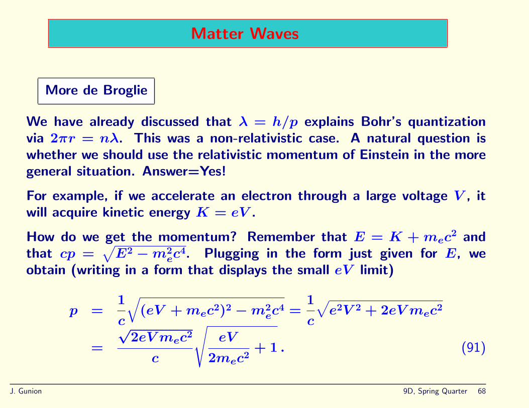
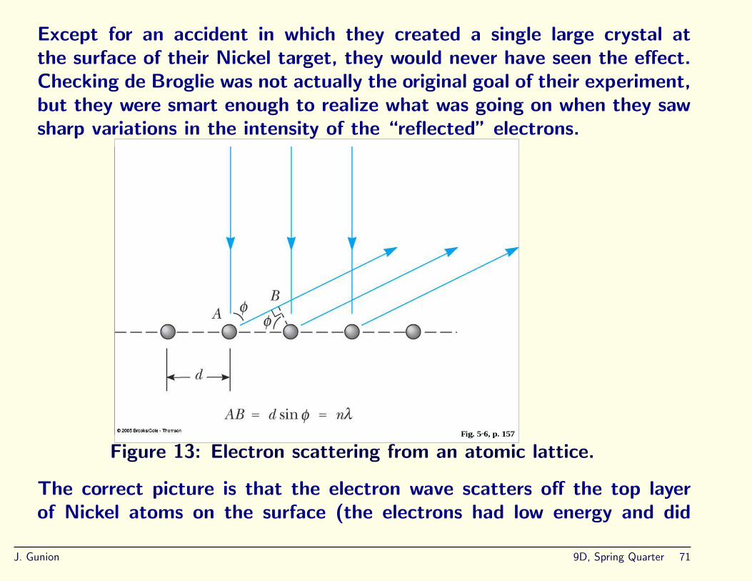
Figure 13: Electron scattering from an atomic lattice.

The correct picture is that the electron wave scatters off the top layerof Nickel atoms on the surface (the electrons had low energy and did


not penetrate beyond the surface). Because these were part of a singlecrystal, they had a very regular spacing, as depicted in the figure.

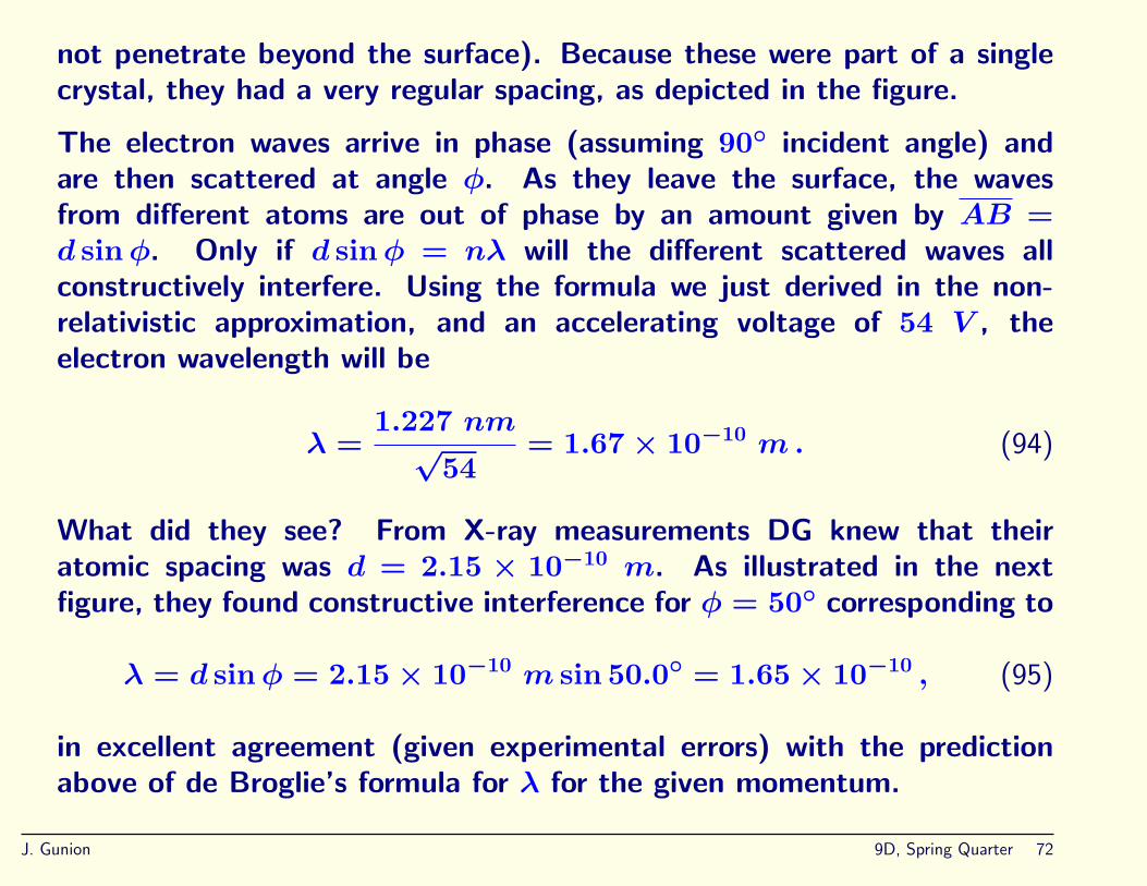
The electron waves arrive in phase (assuming 90◦ incident angle) andare then scattered at angle φ. As they leave the surface, the wavesfrom different atoms are out of phase by an amount given by AB =d sinφ. Only if d sinφ = nλ will the different scattered waves allconstructively interfere. Using the formula we just derived in the non-relativistic approximation, and an accelerating voltage of 54 V , theelectron wavelength will be

λ =1.227 nm

√54

= 1.67 × 10−10 m. (94)

What did they see? From X-ray measurements DG knew that theiratomic spacing was d = 2.15 × 10−10 m. As illustrated in the nextfigure, they found constructive interference for φ = 50◦ corresponding to

λ = d sinφ = 2.15 × 10−10 m sin 50.0◦ = 1.65 × 10−10 , (95)

in excellent agreement (given experimental errors) with the predictionabove of de Broglie’s formula for λ for the given momentum.


Fig. 5−5, p. 156

Figure 14: Scattered intensity vs. scattering angle for 54 eV electronsincident at 90◦.

If one employs higher acceleration voltages, then the e− will penetratefurther into the surface, and the e− waves will see many layers of thecrystal structure. The picture is below.


D cos θθD θ

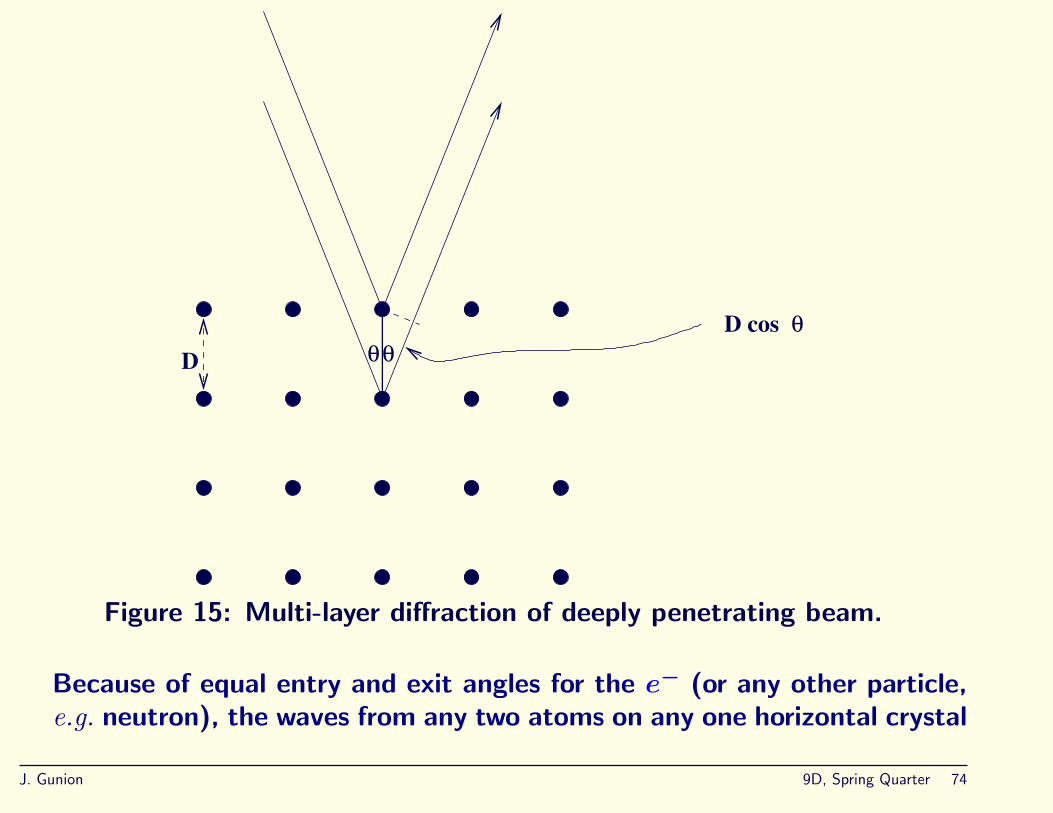
Figure 15: Multi-layer diffraction of deeply penetrating beam.

Because of equal entry and exit angles for the e− (or any other particle,e.g. neutron), the waves from any two atoms on any one horizontal crystal


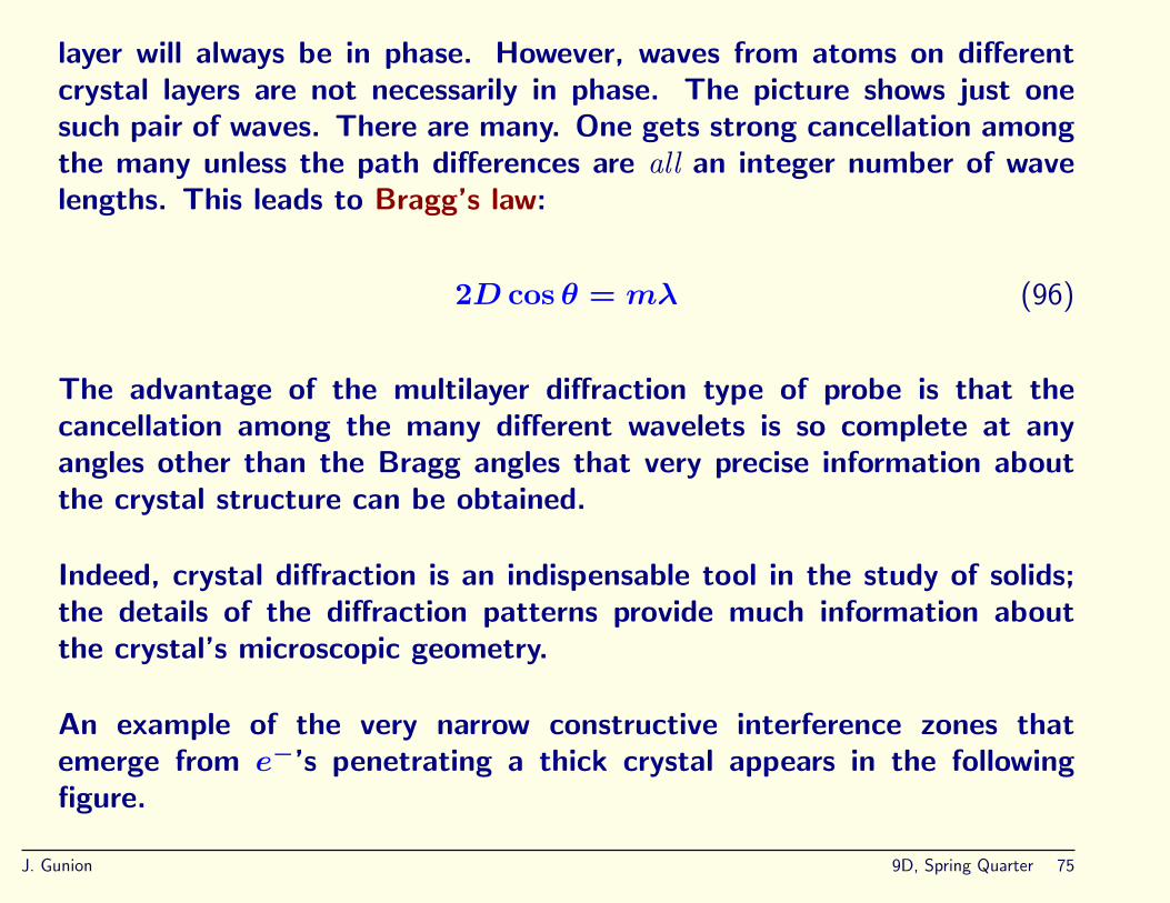
layer will always be in phase. However, waves from atoms on differentcrystal layers are not necessarily in phase. The picture shows just onesuch pair of waves. There are many. One gets strong cancellation amongthe many unless the path differences are all an integer number of wavelengths. This leads to Bragg’s law:

2D cos θ = mλ (96)

The advantage of the multilayer diffraction type of probe is that thecancellation among the many different wavelets is so complete at anyangles other than the Bragg angles that very precise information aboutthe crystal structure can be obtained.

Indeed, crystal diffraction is an indispensable tool in the study of solids;the details of the diffraction patterns provide much information aboutthe crystal’s microscopic geometry.

An example of the very narrow constructive interference zones thatemerge from e−’s penetrating a thick crystal appears in the followingfigure.


Fig. 5−7, p. 157

Figure 16: Bragg diffraction of 50 keV electrons from a 4000 nm thicksingle crystal of CU3Au.

More Examples


(I) If moving with v = 300 m/s, what would be the wavelength (a) of an18, 000 kg airplane, and (b) of an electron?

Answer:

λairplane =6.63 × 10−34 J · s

(18000 kg)(300 m/s)= 1.23 × 10−40 m

λelectron =6.63 × 10−34 J · s

(9.11 × 10−31 kg)(300 m/s)= 2.43 × 10−6 m.(97)

The latter is something you can hope to measure using the kind oftechniques just described. The former is not something you could evermeasure — we do not need to worry about wavelengths and wave patternsin our everyday world!

(II) Consider a two-slit experiment using electrons. The slits are assumedto be very narrow compared to the wave-length of the electrons. Beyondthe slits is a bank of e− detectors. At the center detector, directly in thepath the beam would follow if unobstructed, 100 electrons per secondare detected. Suppose that as the detector angle varies, the number per


unit time of e−’s arriving varies from a maximum of 100/s to a minimumof 0. Suppose the electrons have K = 1.0 eV of kinetic energy and thenarrow slits are separated by S = 0.020 µm. (a) At what angle, θX, isthe detector X located where the minimum is reached? (b) How manyelectrons would be detected per second at the center detector if one ofthe slits were blocked? (b) How many electrons would be detected persecond at the center detector and at detector X if one of the slits werenarrowed to 36% of its original width?

Answers:

(a) At the minimum, we require S sin θX = 12λ. We need, λ = h

p= h

mv

and we get v from

K =1

2mev

2 , ⇒ (1 eV )×(1.6×10−19 J/eV ) =1

2(9.11×10−31 kg)v2

(98)which gives v = 5.93 × 105 m/s. From this we get

p = mv = (9.11×10−31 kg)(5.93×105 m/s) = 5.40×10−25 kg·m/s ,(99)


and

λ =h

p=

6.63 × 10−34 J · s5.40 × 10−25 kg ·m/s

= 1.23 × 10−9 m. (100)

Inserting this into our requirements gives

sin θX ∼ θX =1

2

(1.23 × 10−9 m

0.020 × 10−6 m

)= 0.031 or 1.76◦. (101)

(b) In the discussion that follows, we do not write the wave form explicitly.But, there is always a wave form present. In the present case of e−

waves the wave form would be something like

Aei(kx−ωt) = A [cos(kx− ωt) + i sin(kx− ωt)] , (102)

initially, i.e. before passing through a slit, and would afterwards be similarin form with kx− ωt replaced by kr − ωt, where r is the distance froma slit. The important point will be that whatever the wave form, thetwo slits will have equivalent wave forms, that are in phase at a central


detector location, or exactly out of phase at the first minimum. Thefluxes referred to below can be thought of as the average intensity of theoscillating waves.

With both slits open, the electron flux (electrons per second) is 100/sat the central detector. But, the electron flux is proportional to theprobability of detection and therefore to the square of the amplitude ofthe total matter wave (from both slits):

|ΨT |2 ∝ 100/s ⇒ |ΨT | ∝ 10 . (103)

Since the two slits are very narrow and the waves from the two slits addequally at this point of constructive interference, the amplitude of eitherindividual wave must be half the total:

|Ψ1| ∝ 5 ⇒ |Ψ1|2 ∝ 25/s . (104)

With one slit closed, the electron flux at the central detector would be1/4 the two slit flux, or 25/s. Note the importance of assuming that theslits are really narrow. In this case, this same flux would apply for all theelectron detectors, regardless of angle, when only one slit is open.


You might say, what happened to conservation of probability, or of the numberof photons?. We have not violated anything here. The 100/s when bothslits are open applies only to the central detector. As one movesaway from the central detector, the intensity varies (see E&M two-slitdiscussion) from a maximum of 100 to a minimum of 0 so that averagingover the screen we get 50/s. This is precisely 2× the single-slit uniformintensity, as required by photon number conservation!

(c) If one slit were open and its width (already very narrow) were reducedto 0.36 of its original size, all detectors would register an electron fluxthat is 0.36 × 25/s, or 9/s. In equation form, this means that

|Ψ′1|

2 = 0.36 × |Ψ1|2 ∝ 0.36 × 25/s = 9/s , ⇒ |Ψ′1| ∝ 3. (105)

This is 60% of the original amplitude.

With both slits open (but with slit #1 at only 36% of its original size),we have two waves of different amplitudes, one proportional to 5 (slit#2 of original width) and one proportional to 3 (slit #1). At points ofconstructive interference, such as the central detector, where the waves


add, the total amplitude will be ∝ 5 + 3:

|Ψ′T |constructive ∝ 8 , ⇒ |Ψ′

T |2constructive ∝ 64/s. (106)

At points of previously complete destructive interference, where the twowaves are 180◦ out of phase, such as at detector X, the cancellationwould no longer be complete. The waves still come in with oppositesigns for the amplitudes so that the amplitude is proportional to 5 − 3,leading to

|Ψ′T |destructive ∝ 2 , ⇒ |Ψ′

T |2destructive ∝ 4/s . (107)

The average electron flux is

1

2(64/s+ 4/s) = 34/s , (108)

i.e. the sum of the 9/s and the 25/s expected from each slit alone.

To repeat, to find the probability (or flux) at a given location, we donot add the probabilities (or fluxes) from each slit at that location; these


are always positive, so they cannot cancel. Rather, we add the waveamplitudes, which may add constructively or destructively, to find thetotal wave, and then square the total wave to find the probability.

*** There is a special problem assigned to cover this material: see webpage. You will be tested on some quiz or exam on this kind of thing. ***

The electron microscope and related devices

Recall the formula for the e− wavelength in terms of the accleratingvoltage

λe =1.227 nm√V (volts)

1√eV

2mec2+ 1

. (109)

An electron microscope makes use of an accelerating voltage of V ∼100000 volts, leading to λe ∼ 0.003 nm, as compared to typicallight wavelengths in the visible spectrum of ∼ several hundred nm.Thus, electrons have the potential of far greater resolution capable ofrevealing much finer structures. Magnification, however, is not directlyrelated to λ, being limited by other things such as appertures and“optics” of the device. In practice, the best that can be achieved is


a magnification of 10,000 to 100,000 with resolution of 0.2 nm, ascompared to magnification and resolution of ∼ 2000 and ∼ 100 nm foroptical microscopes. The electron microscope allows pictures of individualDNA strands, bacteria and the like. These developments were crucial tomodern biology, ....

Other devices include scanning electron microscope (SEM) and scanningtunneling microscope (STM) and atomic force microscope (AFM). Theseinvolve further applications of QM to which we shall turn in later chapters.

The latest device for studying structures, especially of germanium crystalsand other semi-conductors, is a light source of very high energy γ-rays.These are beams of photons with energies beyond even the X-ray range.Typical energy is ∼ 10 to 50 × 109 eV . The wavelength that one istalking about is

λ =ch

E∼

1.24 × 103 eV · nm10 × 109 eV

= 1.24 × 10−7 nm . (110)


More on the Heisenberg Uncertainty Principle

Let us review once more the HUP. We have found by example that for anywave pattern it is always true that

∆k∆x ≥1

2, (111)

where I have stated that the minimum arises for Gaussian wave packets.

We then input either Planck (photons) or de Broglie (matter waves) viathe relation

p =h

λ= h

2π

λ= hk , ⇒ ∆p∆x ≥

1

2h . (112)

Another uncertainty relation involves the uncertainty in energy of a wavepacket, ∆E, and the time, ∆t, taken to measure that energy. UsingGaussian or other wave forms that are functions of kx− ωt and that areof finite extent in ∆t, we can derive the wave result that

∆ω∆t ≥1

2, (113)


where once again the minimum is for Gaussian forms.

We now input the relation

E = hf = h(2πf) = hω , ⇒ ∆E∆t ≥1

2h . (114)

This result states that the precision with which we can know the energyof some system is limited by the time available for measuring the energy.

The Mechanistic Point of View of the HUP

∆px∆x

Here we consider an idealized (thought) experiment in which we tryto measure the position of a particle using photons. A more carefultreatment is given in the book. Here, I just give the idea of theargument.

• The photon carries momentum given by p = hλ.

• The matter particle tends to pick up some portion of this momentum(depending upon angle of incidence which is determined by size of lens


of microscope employed — see book) so

(∆p)particle being probed ∼h

λ. (115)

• Also, the position of the particle can not be determined to any greaterprecision than the wavelength λ of the light:

(∆x)particle being probed >∼ λ . (116)

• Multiplying, we get

(∆p∆x)particle being probed >∼ h . (117)

This shows in a mechanistic way that any attempt to improve yourmeasurement of ∆x by employing smaller λ necessarily increases theamount of momentum that the photon will typically transfer to theparticle being probed (the direction being unpredictable) as a result ofthe higher momentum being carried by each photon.

The key physics ideas that lead to the uncertainty principle from themechanistic point of view are:


1. There is an indivisible nature of the light particles (photons) andnothing less than one photon can be used to perform a measurementof the momentum or energy of another particle.

2. There is a wave nature of light that even a single photon cannot evade.3. These lead to the impossibility of predicting or measuring the precise

(classical) path that a single scattered photon will follow, which in turnimplies inability to determine precisely the momentum transferred tothe electron.

∆E∆t

A similar argument is possible for the ∆E∆t relation.

• Consider a wave of frequency f incident on a particle at rest.• Suppose that the minimum uncertainty in the number of waves we can

count is 1 wave.Since f = # we count

time interval, we get

∆f =1

∆t, (118)

where ∆t is the time interval available for counting the waves.


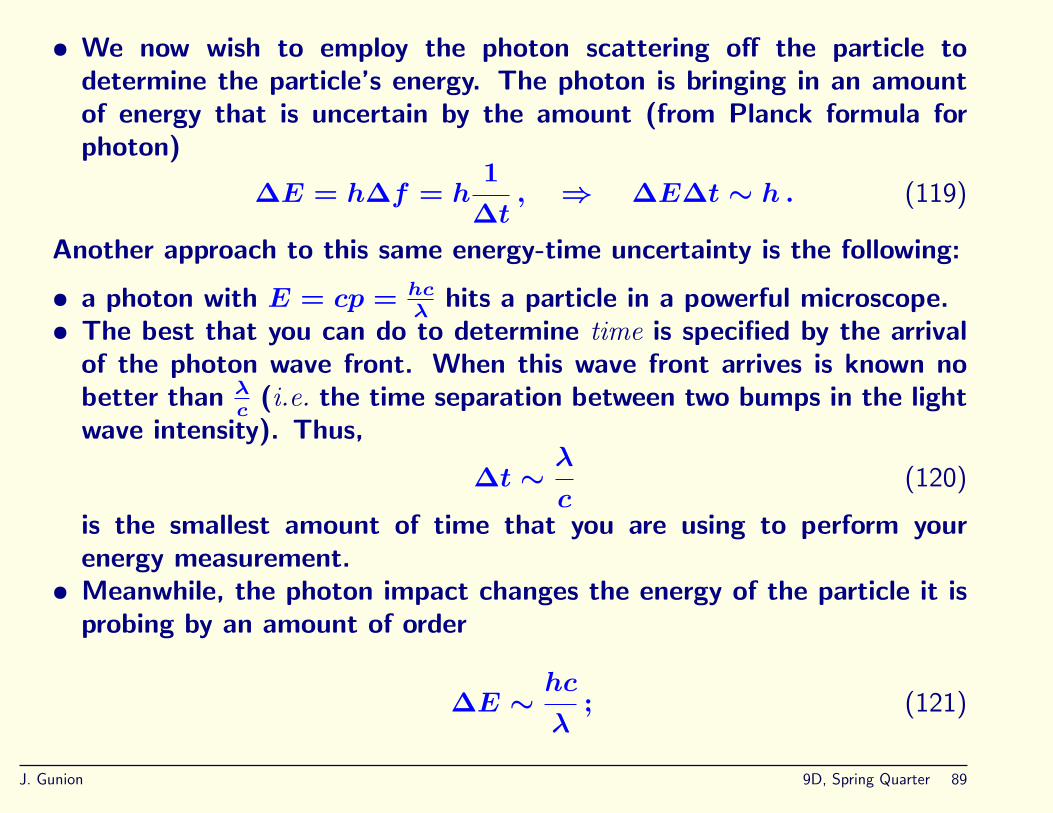
• We now wish to employ the photon scattering off the particle todetermine the particle’s energy. The photon is bringing in an amountof energy that is uncertain by the amount (from Planck formula forphoton)

∆E = h∆f = h1

∆t, ⇒ ∆E∆t ∼ h . (119)

Another approach to this same energy-time uncertainty is the following:

• a photon with E = cp = hcλ

hits a particle in a powerful microscope.• The best that you can do to determine time is specified by the arrival

of the photon wave front. When this wave front arrives is known nobetter than λ

c(i.e. the time separation between two bumps in the light

wave intensity). Thus,

∆t ∼λ

c(120)

is the smallest amount of time that you are using to perform yourenergy measurement.

• Meanwhile, the photon impact changes the energy of the particle it isprobing by an amount of order

∆E ∼hc

λ; (121)


i.e. if you want to not change the energy of the particle the photon isprobing, you must keep λ large. But, then this means it takes longerfor the wave front arrival to be clearly defined. The result is

∆E∆t =hc

λ

λ

c∼ h . (122)

Heisenberg Uncertainty Principle (HUP) Examples

e− in a Hydrogen atom

Is there any relation between the energy levels of the Hydrogen atomand the uncertainty principle? Let’s see.

We suppose that the electron is confined in a one-dimensional senseto a region of order ∆x. Then, let us employ the HUP in the form∆px ∼ h/∆x. (I have chosen the numerical factor to give me theprettiest results.) The associated kinetic energy is

K ≥ (K)∆px ≡(∆px)2

2me

>h2

2me(∆x)2. (123)


Let us demand that this kinetic energy not exceed significantly thenegative potential energy associated with this same distance scale.

(K)∆px ∼h2

2me(∆x)2∼∣∣∣∣−ke2

∆x

∣∣∣∣ . (124)

This gives us,

∆x ∼h2

2kmee2=a0

2. (125)

What this is telling us is that it is very difficult to confine the electron toa distance much smaller than a0 using the electromagnetic force. If wescale up the potential energy using Z for a charged ion, the ∆x cannotdecrease faster than 1/Z without violating the HUP. The same argument

would give us ∆x > a02

1Z. Plugging this into −ke2Z

∆x gives us energy levelsthat should scale as Z2, as they do.

We can actually go further. It is apparent that the typical potentialenergy for an e− confined to a region of size ∆x is

U = −ke2

∆x, (126)


which can be combined with our minimum K for the particle to computethe total energy:

E = K + U =h2

2me(∆x)2−ke2

∆x. (127)

Note that E → 0 for ∆x → ∞, has a minimum somewhere and thenE → +∞ for ∆x → 0. The most likely value of ∆x is the value thatminimizes E. Taking derivatives, this gives

∂E

∂∆x= 0 = −2

h2

2me(∆x)3+

ke2

(∆x)2(128)

which is solved by

∆x =h2

meke2= a0 , (129)

which, after substitution into the above form for E gives

E = −k2e4me

2h2 (130)


which is precisely the E0 energy level of the first Bohr orbit.

The Unstable Z boson

The Z boson is an unstable (i.e. a particle that decays) with massmZ ∼ 91 × 109 eV . The average lifetime of the Z is

τZ = 2.9 × 10−25 s . (131)

This lifetime is determined by how many different types of particles it candecay into and what the strengths of those decays are. One importanttype of particle is something called a “neutrino”, ν. There are potentiallymany different types of neutrinos. The more Z → νν channels thereare, the shorter the Z lifetime. Since we cannot see ν’s directly (theyare very weakly interacting and have zero charge), it is important todetermine the Z lifetime to indirectly determine how many ν’s there are.

However, the above τZ is far too short to actually measure directly. So,how do we determine it. Answer: use Heisenberg uncertainty principlefor theoretically predicted shape of “mass spectrum”.

If we attempt to measure the mass of the Z by using e+e− → Zcollisions with different values of the e+e− total energy, what do we


expect to see? The HUP says we should expect to see a distribution ofmass values of a certain shape.

5

10

15

20

25

30

35

88 89 90 91 92 93 94 95

N=2

N=3

N=4

DELPHI

Energy, GeV

Figure 17: e+e− → hadrons as a function of Me+e−. The Z peak iscentered about mZ = 91.13 × 109 eV = 91.13 GeV and has a width ofroughly 2 to 3 × 109 eV .


The resonance picture shows that we cannot make a precise determinationof the mass. As stated, this is required by the uncertainty principle whichsays that we would need an infinite amount of time to get a precise massdetermination, whereas the resonance disappears quickly. The HUP says

∆E ≡ ∆mZ ∼ h1

τZ=

6.582 × 10−16 eV · s2.9 × 10−25 s

∼ 2.3×109 eV = 2.3 GeV ,

(132)and this is what is explicitly seen in the plot. The plot also shows howthe peak would get narrower (broader), relative to its height, if certaindecay modes are eliminated (added).

Relation of HUP to Two-Slit Interference Pattern

Things we know

Assume equal slit widths.

1. It is only when we have both slits open that the interference patterndevelops.

2. Even if we send only one e− at a time, if both slits are open the e−

hits at the detector bank will accumulate where the interference wave


prediction has a maximum and no e−’s will hit at the destructive wavepattern cancellation minima.

3. We cannot be sure where any given e− will end up; only the finalaverage pattern can be predicted with certainty.

4. If we close one slit, the accumulation pattern changes to approximatelyuniform (for very narrow slits).

Now try to do better.

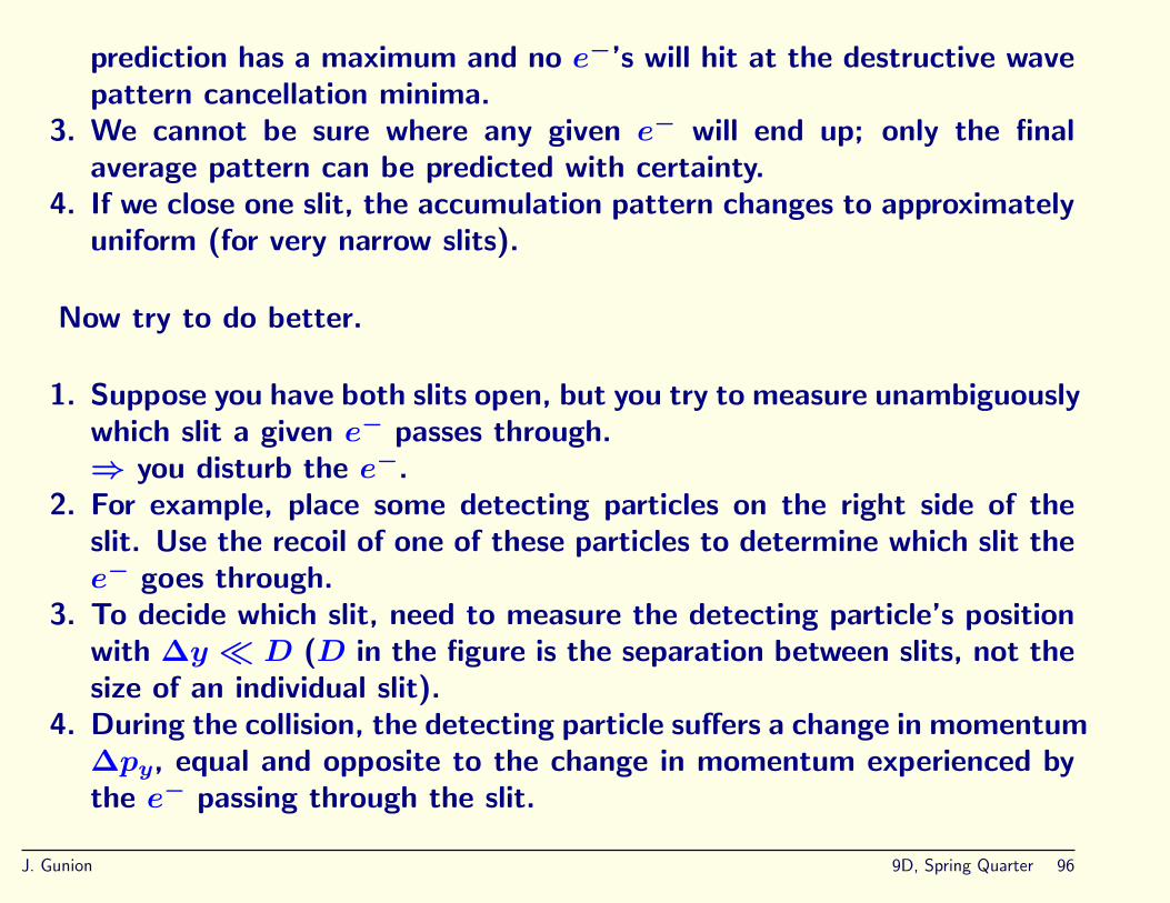
1. Suppose you have both slits open, but you try to measure unambiguouslywhich slit a given e− passes through.⇒ you disturb the e−.

2. For example, place some detecting particles on the right side of theslit. Use the recoil of one of these particles to determine which slit thee− goes through.

3. To decide which slit, need to measure the detecting particle’s positionwith ∆y � D (D in the figure is the separation between slits, not thesize of an individual slit).

4. During the collision, the detecting particle suffers a change in momentum∆py, equal and opposite to the change in momentum experienced bythe e− passing through the slit.


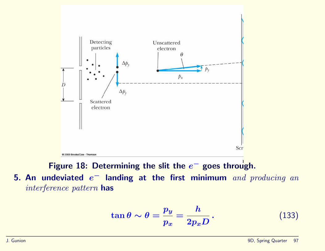
Fig. 5−33, p. 184Figure 18: Determining the slit the e− goes through.

5. An undeviated e− landing at the first minimum and producing aninterference pattern has

tan θ ∼ θ =py

px=

h

2pxD. (133)


(This is our old 12λ path difference requirement.)

6. Thus, we require that an e− scattered by a detecting particle has

∆pypx

� θ =h

2pxDor ∆py �

h

2D(134)

if the interference is to not be distorted.7. Because

(∆py)e− = −(∆py)detecting particle , (135)

(∆py)detecting particle �h

2D(136)

is also required.8. Altogether, for the detecting particle, we require

(∆py∆y)detecting particle �h

2D·D =

h

2. (137)

This is in clear violation of the uncertainty principle.If ∆y is small enough to determine which slit the electron goes through,∆py will be so large that the e−’s will be deflected all over the placeand the interference pattern will be destroyed.


Matter Probability Waves and the SchroedingerEquation

I will be, and have been for that matter, kind of combining the materialappearing in Chapters 5 and 6. You should read this material as a unit. Forexample, I have set up the ingredients for writing down the Schroedingerequation that first appears in Sec. 6.3, where it is introduced more or lessby fiat. I will now go a little bit beyond just simply writing it down and tellyou one way that you can kind of understand it.

The Schroedinger Equation

The Schroedinger equation is the wave equation for matter probabilitywaves when the non-relativistic limit is appropriate. A different equationmust be used if the matter particles are in a situation where they typicallyhave relativistic velocities.

Recall the game we played for “deriving” the light-wave equations.We wrote E2 = c2p2, multiplied this equation by some Ey or Bz


electromagnetic field and then replaced

px =h

i

∂

∂x, E = ih

∂

∂t. (138)

In this case, we write (non-relativistically and neglecting any potentialsor such for the moment — i.e. we consider a “free” particle)

E = m0c2 +

p2

2m, ⇒ EΨ =

(m0c

2 +p2

2m

)Ψ

⇒ ih∂Ψ

∂t= m0c

2Ψ −h2

2m0

∂2Ψ

∂x2. (139)

In the text, the constant m0c2 is absorbed into an overall redefinition of

the energy scale in this NR limit, but this is really misleading when itcomes to considering how the particle is moving, as we shall see.

The very simplest solution to this equation is the exponential form:

Ψ = Aei(kx−ωt) , (140)


where we compute ω(k) from the SE (Schroedinger equation) requirement

ih(−iω(k))Aei(kx−ω(k)t =(m0c

2 − h2(ik)2)Aei(kx−ω(k)t) , (141)

implying

ω(k) =m0c

2

h+hk2

2m. (142)

Note how this is consistent with the de Broglie / Planck relations

k =2π

λ=

2πp

h=p

h, and ω = 2πf = 2π

E

h=E

h(143)

or equivalently

p =h

λ= h

2π

λ= hk , E = hf = h2πf = hω (144)

being substituted into E = m0c2 + p2/2m:

E = hω = m0c2 +

(hk)2

2m0. (145)


The m0c2/h part of ω(k) is normally dropped in the non-relativistic limit,

as it amounts to an irrelevant redefinition of the absolute energy scale.In the relativistic limit, it cannot be dropped.

Note that a sin or cos function form does not solve the SE. For example,if we tried the sin function form, the single time derivative would giveus a cos function, whereas the double space derivative would give usback − sin. In the free-particle case at any rate, we must employ theintrinsically complex “plane wave” form

Aei(kx−ωt) = A cos(kx− ωt) + iA sin(kx− ωt) . (146)

This is still a traveling complex wave moving in the +x direction becauseof the kx − ωt argument which says that if I move in the direction xby an amount ∆x then I can compensate by advancing t by an amount∆t = k∆x/ω. We shall soon consider whether the velocity that youmight compute from

∆x

∆t=ω(k)

k=m0c

2

hk+

hk

2m0=m0c

2

p+

p

2m0(147)

has any meaning. The answer is no. We will have to deal with wave


packets and the concepts of phase and group velocity to which we shortlyturn.

The HUP (again).

As stated, the above ei(kx−ωt) solution to the SE is called a plane wavesolution.

The particle described by this solution has a precisely defined momentum(in the x direction) of p = hk, as computed above.

If the HUP is correct, ∆x should be infinite! and it is!

This is because

|Ψ|2 = A2 (148)

is completely independent of x and so the particle has a uniformprobability of being anywhere along the x axis! Obviously, it is nonsenseto discuss the velocity of a uniform probability distribution.


How fast is the matter particle moving?

We must now face the subtle issue of how to construct a wave formthat can describe an actual physical particle and how it is we determinethe velocity of the particle. This will bring us to consider the differencebetween group and phase velocity.

We considered in Fig. 8 and surrounding material how to create a photon-like object by adding together E&M type wave patterns. There, thegroup and phase velocities were both equal to c and we did not distinguishor even discuss. For massive particles one must be careful.

The book has a discussion using two sin waves. However, I prefer touse the plane wave form we have just been discussing, which is an actualsolution of the SE (unlike the sin or cos forms alone).

To define a “particle” we clearly cannot use a single plane-wave solutionfor which the particle has no preferred location.

We must superimpose a least two plane-wave solutions.

Let us begin with exactly two and see what happens.


• WriteΨ(x, t) = Aei(k1−ω1t) +Aei(k2−ω2t) (149)

where we have taken in to account the fact that when k changes alittle bit then so must ω.

• Let us assume we only change k by a small amount and write

k1 = k0 + dk , k2 = k0 − dk , ω1 = ω0 + dω , ω2 = ω0 − dω .(150)

• Then,

Ψ = A[ei[(k0+dx)x−(ω0+dω)t] + ei[(k0−dx)x−(ω0−dω)t]

]= Aei(k0−ω0t)

[ei[(dk)x−(dω)t] + e−i[(dk)x−(dω)t]

]= Aei(k0x−ω0t)2 cos [(dk)x− (dω)t] . (151)

• We have a complex exponential that moves at speed

vp ≡ω0

k0=hω0

hk=E0

p0, (152)


where vp is called the phase velocity appropriate to these centralvalues, modulated by a cosine function that moves at speed

vg ≡dω

dk, (153)

which is called the group velocity.• It is this latter term that defines the envelope of the wave and tells us

where the probability is. Indeed,

|Ψ|2 = 4A2 cos2 [(dk)x− (dω)t] . (154)

The phase velocity has disappeared. Since a physical particle moveswith its probability, the actual physical speed of the particle is vg.

• Of course, this two-plane-wave superposition is still a bit too simple.It is really a sequence of peaks that we observe passing by. To get alocalized wave form we have to form the kind of superposition discussedearlier:

Ψ(x, t) =∫ ∞

−∞ψ(k)ei(kx−ω(k)t)dk . (155)

We will do another explicit construction of this type shortly. Theimportant point is that since the sum must include plane waves of


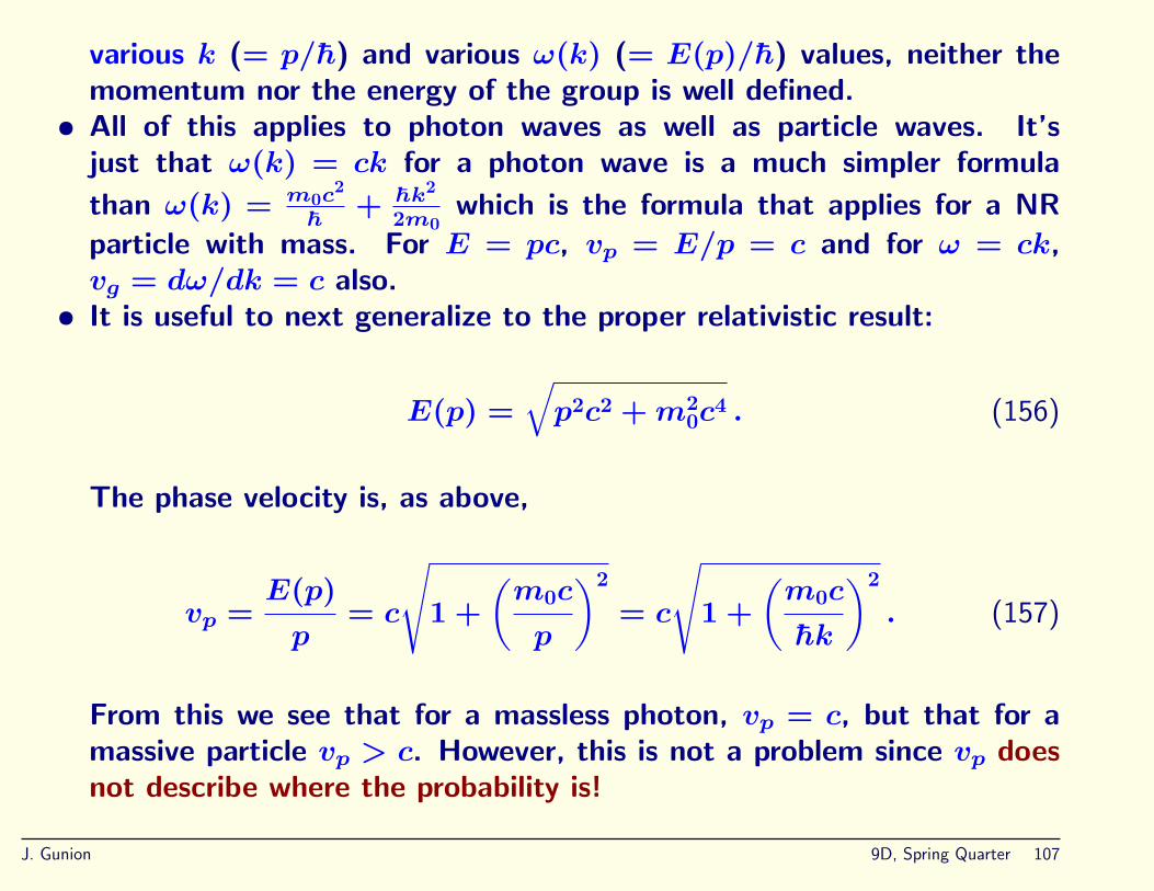
various k (= p/h) and various ω(k) (= E(p)/h) values, neither themomentum nor the energy of the group is well defined.

• All of this applies to photon waves as well as particle waves. It’sjust that ω(k) = ck for a photon wave is a much simpler formula

than ω(k) = m0c2

h+ hk2

2m0which is the formula that applies for a NR

particle with mass. For E = pc, vp = E/p = c and for ω = ck,vg = dω/dk = c also.

• It is useful to next generalize to the proper relativistic result:

E(p) =√p2c2 +m2

0c4 . (156)

The phase velocity is, as above,

vp =E(p)

p= c

√1 +

(m0c

p

)2

= c

√1 +

(m0c

hk

)2

. (157)

From this we see that for a massless photon, vp = c, but that for amassive particle vp > c. However, this is not a problem since vp doesnot describe where the probability is!


• Instead, we must look at vg = dω/dk. We have (using our time-testedrelation f = E/h)

ω(k) = 2πf =E(p = hk)

h=

1

h

√h2k2c2 +m2

0c4 ,

⇒vg =

dω(k)

dk=

1

h

h2kc2√h2k2c2 +m2

0c4

=c√

1 +(m0chk

)2 =c2

vp, (158)

implying that vg < c, given that vp > c as just derived above.• We can now check that vg is the actual speed of the particle by using

vp =E

p=γ(u)m0c

2

γ(u)m0u=c2

u⇒ vg =

c2

vp= u ! (159)

More on wave functions and propagating waves


It was Max Born who in 1925 zeroed in on the interpretation of Ψ as aprobability amplitude.

He had in mind in particular the case where we want to describe a singleparticle that is sufficiently localized (unlike our nice plane wave solution,more like our wave packet type solutions) that you can (and should)define a normalizable probability. Then, he said that

P (x)dx = |Ψ(x, t)|2dx (160)

should be the probability that the particle will be found in the infinitesimalinterval dx about the point x. Once again, I stress that Ψ itself isnot something you can observe and even |Ψ|2 is only observable in aprobabilistic sense.

Because of its relation to probabilities, we will typically insist on thefollowing.

1. Ψ should be single valued and a continuous function of x and t. In thisway, no ambiguities will arise concerning the predictions of the theory.

2. In fact, we will typically require that not only should Ψ be continuous,but it should also be smooth in the sense that its first derivatives arefinite.


However, there are certain specialized situations where this is notappropriate. But, for most of the physical situations we shall discussin this course, this requirement should be met. The exception is whenthere is some discontinuity in some potential.

3. Next, the total probability of finding a particle somewhere should beunity. Since |Ψ|2 is the probability distribution for the particle inquestion, this means∫ ∞

−∞|Ψ(x, t)|2dx = 1 for any t . (161)

Similarly,

Pab =∫ b

a

|Ψ(x, t)|2dx (162)

should be the probability of finding the particle in the interval a ≤ x ≤b.

In this formulation of QM, the fundamental problem of QM is thefollowing: Given the wavefunction at some initial instant, say t = 0, whatis the wavefunction at any subsequent time t.

To answer this question requires a dynamical equation for Ψ(x, t). We


have already written this dynamical equation down. It is Schroedinger’s(wave) equation.

We have discussed it in the free-particle case, mostly focusing on thefree-particle plane wave solution. However, the function Ψ = Aei(kx−ωt)

is not normalizable in the way we would like. There is uniform probabilityeverywhere.

However, we have also learned how to proceed. We form an appropriatesuperposition of plane waves, sometimes called a wave packet. As statedearlier, the Gaussian type of superposition is the most ideal. Let us gothrough the details now.

1. We start with

Ψ(x, 0) =∫ ∞

−∞Ψ(k)eikxdk (163)

with Ψ(k) = (Cα/√π) exp[−α2k2].

Since Ψ(k) is centered about k = 0, we will be constructing a wavepacket that has a central momentum and velocity of 0 (motionlessparticle), although there will be a spread of velocities and momentaabout this central value.

2. We can perform the k integral if we carefully examine it and use the


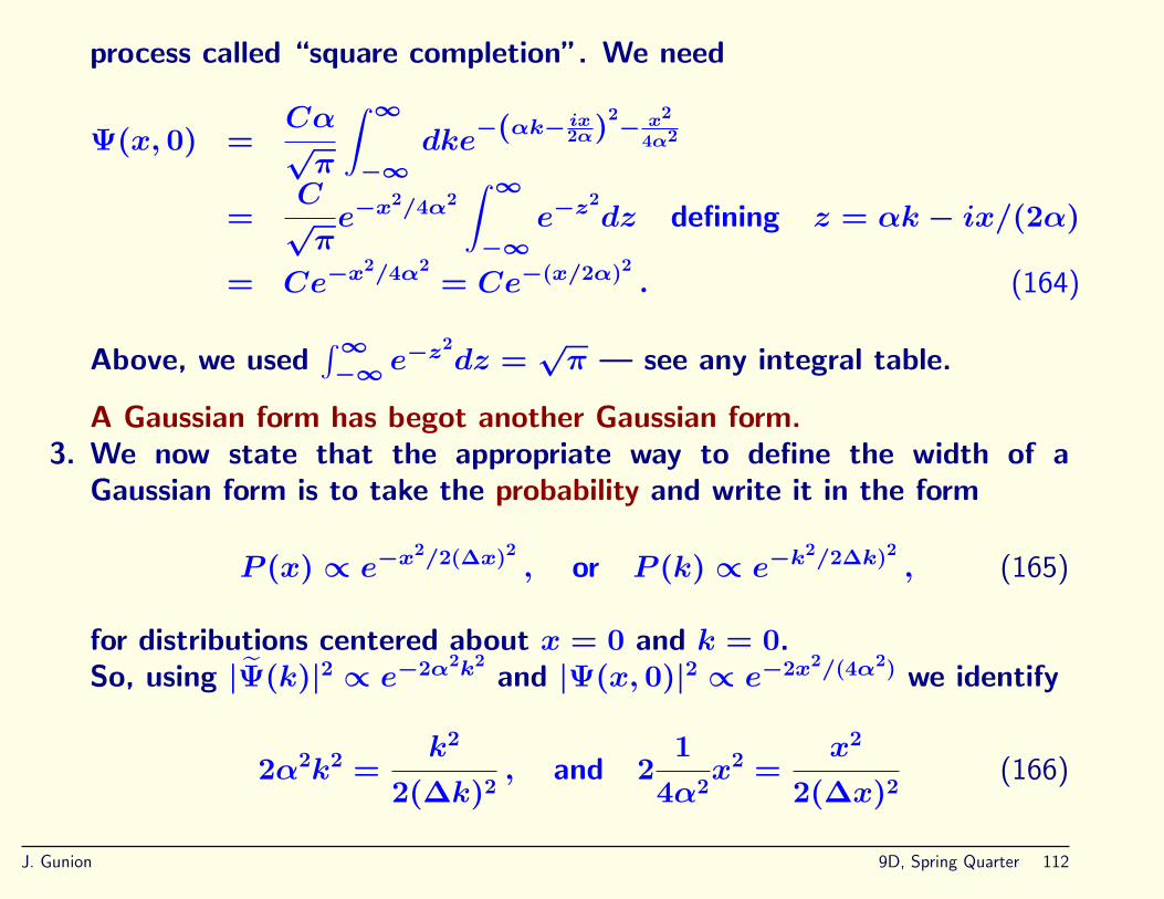
process called “square completion”. We need

Ψ(x, 0) =Cα√π

∫ ∞

−∞dke

−(αk− ix2α)

2− x2

4α2

=C

√πe−x2/4α2

∫ ∞

−∞e−z2

dz defining z = αk − ix/(2α)

= Ce−x2/4α2= Ce−(x/2α)2 . (164)

Above, we used∫∞

−∞ e−z2dz =

√π — see any integral table.

A Gaussian form has begot another Gaussian form.3. We now state that the appropriate way to define the width of a

Gaussian form is to take the probability and write it in the form

P (x) ∝ e−x2/2(∆x)2 , or P (k) ∝ e−k2/2∆k)2 , (165)

for distributions centered about x = 0 and k = 0.So, using |Ψ(k)|2 ∝ e−2α2k2

and |Ψ(x, 0)|2 ∝ e−2x2/(4α2) we identify

2α2k2 =k2

2(∆k)2, and 2

1

4α2x2 =

x2

2(∆x)2(166)


from which we find

∆k =1

2α, and ∆x = α , (167)

implying ∆k∆x = 12. That these are the appropriate definitions of

∆k and ∆x will be left until a later time. But, assuming this, we areback to our minimum HUP after multiplying by h and converting top = hk.

4. Finally, we can normalize this Ψ(x, 0) by requiring

1 =∫ ∞

−∞|Ψ(x, 0)|2dx

=∫ ∞

−∞C2e−2x2/4α2

dx

= C2(√

2α)∫ ∞

−∞e−y2

dy using y = x/(√

2α)

= C2(√

2α)√π , ⇒ C =

1

(2π)1/4√α, (168)

where we have claimed that α = ∆x for an appropriate definition of∆x.


We should now discuss how it is that this wavepacket evolves with time.

We find that it disperses, getting broader in space as time passes. Thisis because it was initially made up of plane waves with many different kvalues (both positive and negative).

The steps and results are as follows:

1. For t 6= 0, use

Ψ(x, t) =∫ ∞

−∞Ψ(k)ei(kx−ω(k)t)

=∫ ∞

−∞Ψ(k)e

i

(kx− hk2

2met

)dk

=C

√π

∫ ∞

−∞e−α2k2+ikx−ihtk2/(2me)dk (169)

where we inserted the expression for ω(k) that is required by Schroedinger’sequation.

2. We can again complete the square. In the exponent we have


ikx− k2[α2 + iht/(2me)]

= −

k√α2 +

iht

2me

−ix

2√α2 + iht

2me

2

−x2

4(α2 + iht

2me

) .(170)

I will not go through the details of the variable shift and integration.The fact that the k2 coefficient is complex is not any particularproblem. You just have to trust your square completion process anduse the standard

∫∞−∞ exp[−y2]dy =

√π at the appropriate point.

3. The important component of interest is the residual coming from thelast term above which says that

Ψ(x, t) ∝ exp

−x2

4(α2 + iht

2me

) . (171)

4. As always, in defining a width we are interested in the probability and


not the amplitude. We have

|Ψ(x, t)|2 ∝ exp

[−1

4

x2

α2 + iht2me

]× exp

[−1

4

x2

α2 − iht2me

]= exp

[−1

4x2(

1

α2 + iht/(2me)+

1

α2 − iht/(2me)

)]

= exp

−14x

2

2α2

α4 +[ht

2me

]2

= exp

−1

2

x2

α2 +[ht

2meα

]2

≡ exp[−

1

2

x2

[∆x(t)]2

]⇒ [∆x(t)]2 = [∆x(0)]2 +

[ht

2me∆x(0)

]2, (172)

where we used α = ∆x(0). In getting from the 2nd to the 3rd line


above, we used1

a+ ib+

1

a− ib=

2a

a2 + b2. (173)

Non-stationary case

If we want a particle whose central location is moving, we simply modifyour input form of Ψ(k) so that it is a Gaussian (or other choice) centeredabout k = k0. The packet would then move with a group velocity given,in the NR case, by

vg =[dω(k)

dk

]k=k0

=[d

dk

(hk2

2m0

)]k=k0

=hk0

m0. (174)

The wave packet would, just as in the k0 = 0 case discussed above, spreadout as time passed due to the presence of a distribution of momenta andvelocities for individual subcomponents of the wave packet.

Definition of ∆x?

So, let us now use the probability interpretation of Ψ(x, 0) to actually


define an appropriate definition of ∆x. We employ (from eq. (164))

P (x) = |Ψ(x, 0)|2 =∣∣∣Ce−x2/4α2

∣∣∣2 = C2e−x2/2α2. (175)

We could then define the average value of x as

〈x〉 ≡∫ ∞

−∞xP (x) dx , ⇒ 〈x〉 = 0 (176)

for the particular form of P (x) above due to the fact that P (x) is evenin x → −x, whereas as x changes sign under x → −x.

We now come to the “standard” definition of ∆x:

(∆x)2 = 〈(x− 〈x〉)2〉 = 〈x2〉 − 2〈x〈x〉〉 + 〈x〉2 = 〈x2〉 − 〈x〉2. (177)

Let us compute 〈x2〉.

〈x2〉 ≡∫ ∞

−∞x2P (x) dx


=∫ ∞

−∞x2C2e−x2/2α2

dx

= C2√

2πα3 using∫∞

−∞ e−ax2dx =

√π/(2a3/2)

= α2 using C2 = 1/(√

2πα) . (178)

Thus, using this definition of ∆x, we do indeed find that ∆x = α asclaimed earlier.

You should remember how we proceeded here. We could compute otheraverage values using P (x), and these will have real physical meaning invarious situations, just as ∆x really describes the size of a wave packetin a quantitative way.

Another example: a structure localized in time

This time, we consider a probability that is somewhat localized in time.In particular, we consider the case of an unstable particle produced att = 0 which then decays according to a probability distribution

P (t) ≡dN

dt= N0e

−t/τ , (179)


where by convention τ is referred to as the particle lifetime.

Of course, we must remember that P (t) is not the amplitude, but ratherthe probability. The amplitude will be f(t) ∝

√P (t) ∝ e−t/2τ .

If we are talking about solutions to the SE, it must be that this timestructure is a superposition of plane-wave type solutions (these are all wehave — they form a complete set). In the case of a time structure, thismeans that there must exist a f(ω) such that

f(t) =∫ ∞

−∞dωf(ω)e−iωt . (180)

The appropriate f(ω) is found by the inverse relation

f(ω) =1

2π

∫ ∞

−∞dteiωtf(t) (181)

as we easily show.

Proof


We use a “dummy” variable t′ to define the f(ω) integral form and thenwrite:

f(t) =?1

2π

∫ ∞

−∞dω

[∫ ∞

−∞dt′eiωt

′f(t′)

]e−iωt

=1

2π

∫ ∞

−∞dt′f(t′) lim

W→∞

∫ W

−Wdωeiω(t′−t)

=1

2π

∫ ∞


W→∞

eiW (t′−t) − e−iW (t′−t)

i(t′ − t)

=1

2π

∫ ∞


W→∞

2 sin[W (t′ − t)]

t′ − t= f(t) . (182)

The last step takes a bit of work. Note that if t′ 6= t then thesin[W (t′ − t)] is very rapidly oscillating as a function of t′ (for very largeW ) and in the large W limit nothing will survive in the

∫dt′ integral

for any tiny dt′ interval where t′ 6= t. Assuming that f(t) is a smoothly


varying function on the scale of 1/W , this allows us to write

1

2π

∫ ∞


W→∞

2 sin[W (t′ − t)]

t′ − t

= f(t)1

2πlimW→∞

∫ ∞

−∞dt′

2 sin[W (t′ − t)]

t′ − t= f(t) , (183)

where for the last step we have simply looked up the integral in a tableand found that its value is 2π independent of t′ − t and W .

QED

So, now let us return to the computation of interest:

f(ω) =1

2π

∫ ∞

−∞dteiωtf(t)

∝1

2π

∫ ∞

0dteiωte−t/2τ

=1

2π

∫ ∞

0dtet(iω−1/2τ )


=1

2π

[et(iω−1/2τ )

iω − 1/2τ

]∞

0

=1

2π

[1

1/2τ − iω

]. (184)

From this we compute the P (ω) distribution as

P (ω) = |f(ω)|2 ∝1

ω2 + 14τ2

. (185)

If we want to make connection with the Z resonance example givenearlier, see Fig. 17, we would write hω = E −mZc

2 and the functionalform given above is precisely that used to draw the plotted curves, one ofwhich fits perfectly (for the correct choice of τ = τZ) the experimentaldata. The quantity h/τ that determines the width of the E distributionis sometimes written as Γ = h/τ . For the precise τZ given earlier wehave

ΓZ =h

τz= 2.3 GeV , (186)

as computed earlier, eq. (132).


The Schroedinger Equation in the Presence ofForces/Potentials

We begin by following our previous route of writing an equation for theenergy, but now including a potential energy term, U(x), which isassociated with a force, F (x) = −dU/dx:

E =p2

2m0+ U . (187)

We will consider only cases where U = U(x). Now, multiply by Ψ(x, t)and make the replacements E → ih ∂

∂t, p → h

i∂∂x

to obtain the SE:

ih∂Ψ(x, t)

∂t= −

h2

2m0

∂2Ψ(x, t)

∂x2+ U(x)Ψ(x, t) . (188)

Although we have motivated the above replacements on the basis of theHUP and wave ideas and analogies to E&M wave regarding momentum


and energy, the SE and the probability interpretation of Ψ must reallybe regarded as a basic new law that we must repeatedly test againstexperiment.

Is there a solution analogous to ei(kx−ω(k)t) to the SE in the presence ofU?

When U does not depend explicitly on t, we can always write

Ψ(x, t) = ψ(x)φ(t) (189)

which is to say the time and space dependence can be separated. (Inthe U = 0 case, ψ(x) = eikx and φ(t) = e−iωt.) Substituting this forminto eq. (188) and dividing by ψφ, we obtain (I will drop the subscript 0on m0, and simply write m in what follows.)

−h2

2m

ψ′′(x)

ψ(x)+ U(x) = ih

φ′(t)

φ(t). (190)

The lhs depends only on x and the rhs depends only on t. This is onlypossible if both sides are equal to the same constant, which we call E


(of course). We can immediately integrate the rhs:

ihdφ(t)

dt= Eφ(t) : ⇒ φ(t) = e−iEh t = e−iωt . (191)

This leaves us with solving the time-independent lhs

−h2

2m

d2ψ(x)

dx2+ U(x)ψ(x) = Eψ(x) , (192)

which is often rewritten in the form

d2ψ

dx2=

2m

h2 [U(x) − E]ψ(x) . (193)

If U = 0, this reduces to our free-particle situation with ψ(x) = eikx

and E = h2k2/(2m). Even in the case of U 6= 0, E will be the totalenergy, and will be a constant describing the state in which the particleresides.

The solution ψ(x) will depend upon U , but for P (x) = |ψ(x)|2 to bephysically interpretable, ψ(x) should be finite everywhere, single-valued


and continuous. Further, ψ(x) should be smooth in that dψdx

should be

normally be continuous. (Just from the SE itself, d2ψdx2 can only be infinite

if U is infinite.)

Finally, note that since |φ(t)|2 = 1, we have

P (x, t) = |Ψ(x, t)|2 = |ψ(x)|2 (194)

which is to say that P (x, t) is independent of time. This is why suchsolutions are referred to as stationary states — all probabilities are static.

Particle in a box

We envision an electron or other particle confined absolutely to a regionbetween x = 0 and x = L by a potential

U(x) ={

0 , 0 ≤ x ≤ L∞ , x < 0 or x > L

. (195)


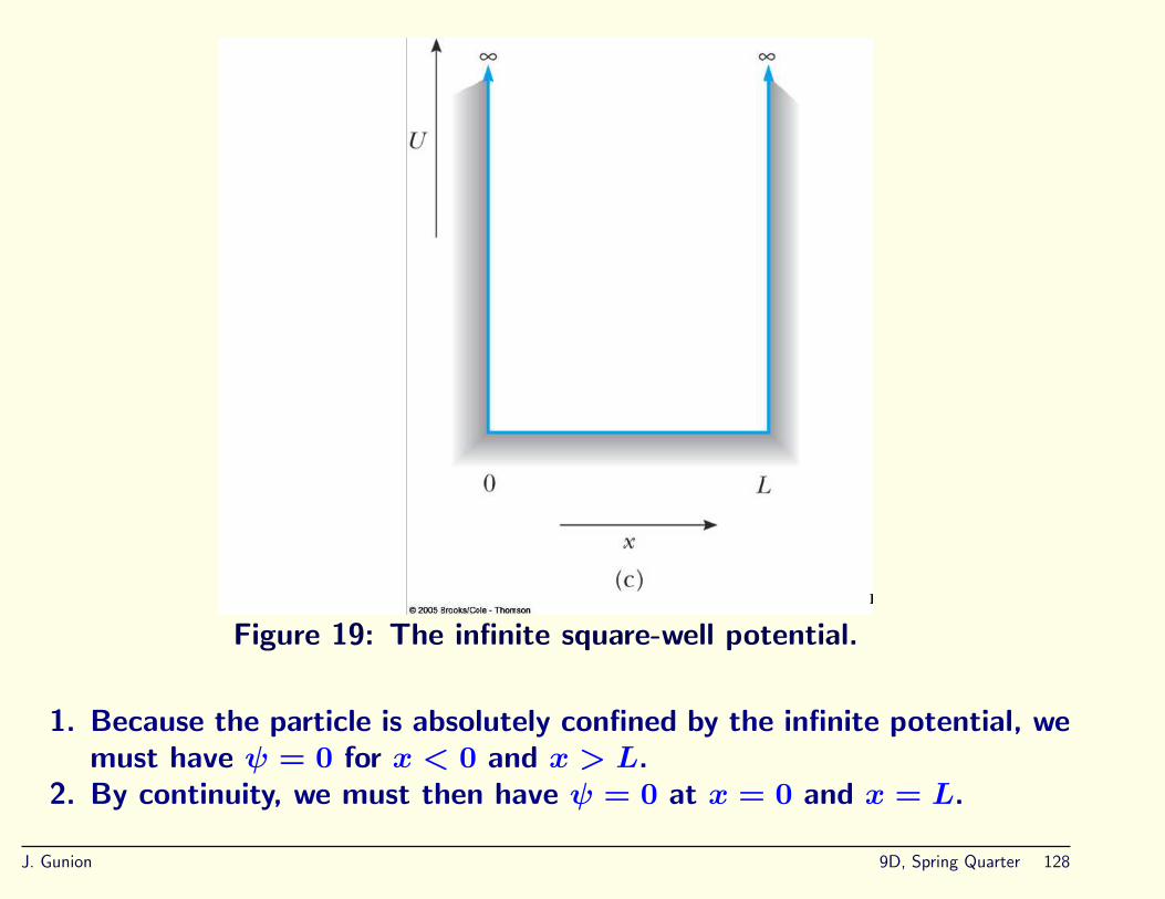
Fig. 6−6c, p. 201

Figure 19: The infinite square-well potential.

1. Because the particle is absolutely confined by the infinite potential, wemust have ψ = 0 for x < 0 and x > L.

2. By continuity, we must then have ψ = 0 at x = 0 and x = L.


3. For 0 ≤ x ≤ L, U = 0 and we must solve (defining E = h2k2/(2m)as usual in the NR case)

d2ψ

dx2= −

2mE

h2 ψ(x) = −k2ψ(x) . (196)

4. The solution can be a combination of sin kx and cos kx:

ψ(x) = A sin kx+B cos kx , for 0 < x < L . (197)

5. At x = 0, ψ(0) = 0 ⇒ B = 0.At x = L, with B = 0, and assuming A 6= 0, ψ(L) = 0 ⇒ kL = nπ.This latter condition can be written in what should now be a not-unexpected manner. Namely:

kL = nπ ⇒ k =nπ

L⇒

2π

λ=nπ

L→

n

2λ = L ,

(198)which is to say that we must fit a half-integer number of wave-lengthsin between the box edges.


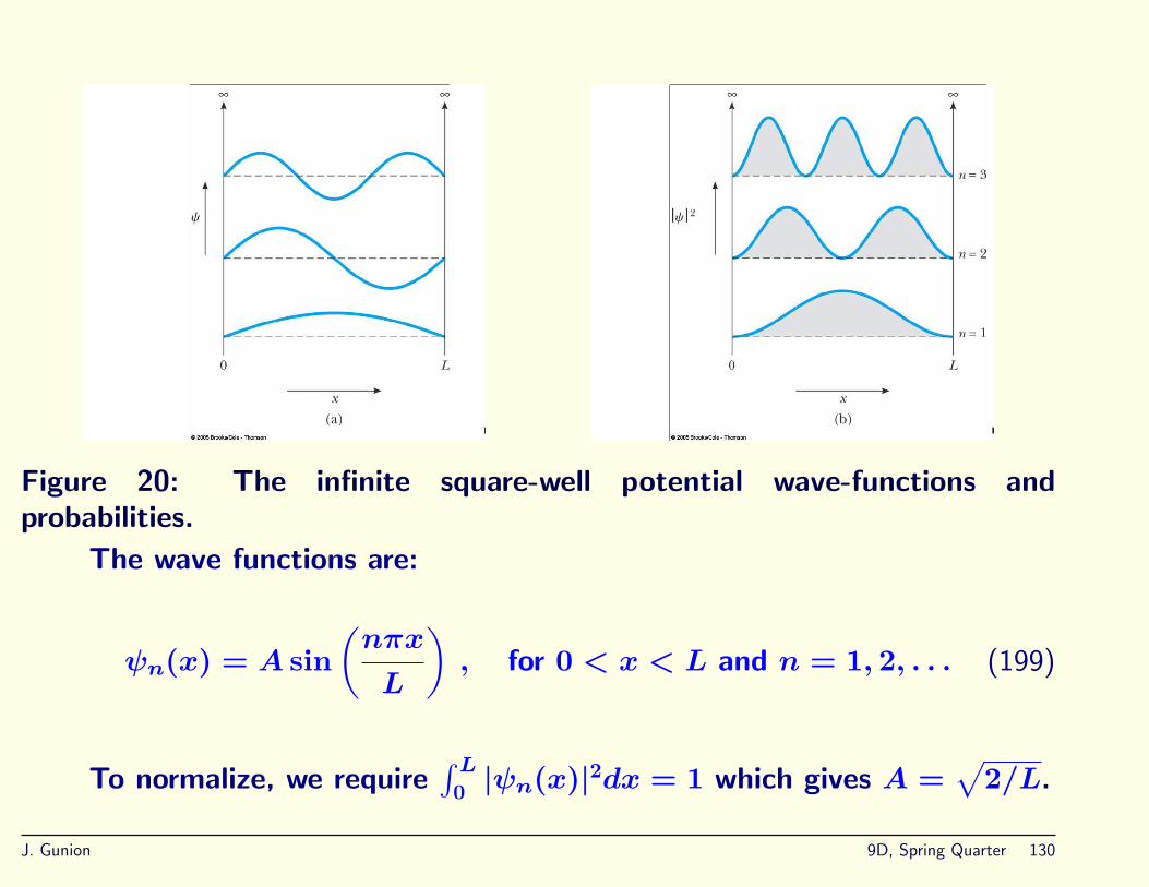
Fig. 6−9a, p. 204 Fig. 6−9b, p. 204

Figure 20: The infinite square-well potential wave-functions andprobabilities.

The wave functions are:

ψn(x) = A sin(nπx

L

), for 0 < x < L and n = 1, 2, . . . (199)

To normalize, we require∫ L0 |ψn(x)|2dx = 1 which gives A =

√2/L.


Figure 21: Scanning tunneling microscope (STM) pictures of electronpatterns in approximately infinite well set ups.

Above, are two pictures of the electron density for two approximatelyinfinite well set ups. For example, the 2nd picture has a one-dimensionaloval well set up. The regular peaks along the ring of atoms that createa “well” like our square well are the STM measurements of the electrondensity. Note the wave pattern. So, you should believe this stuff!


Figure 22: (a) The discovery of the STM’s ability to image variations in the density

distribution of surface state electrons created a compulsion to have complete control of

not only the atomic landscape, but the electronic landscape also. Here we have positioned

48 iron atoms into a circular ring in order to ”corral” some surface state electrons and

force them into ”quantum” states of the circular structure. The ripples in the ring of

atoms are the density distribution of a particular set of quantum states of the corral. The

STM measured distributions agree with those found for the corral by solving the classic

eigenvalue problem in quantum mechanics – a particle in a hard-wall box. (b) Here we have

another STM measurement where iron atoms are shaped into a stadium shaped structure.J. Gunion 9D, Spring Quarter 132

6. The corresponding energy values are:

E =h2k2

2m=n2π2h2

2mL2, n = 1, 2, . . . (200)

Fig. 6−7, p. 202

Figure 23: The infinite square-well potential energy levels.

The lowest energy level is the n = 1 state, which we call the ground


state.

E1 =π2h2

2mL2. (201)

7. Note that n = 0, corresponding to E = 0 is not a possible solution.This means the particle can never be at rest.This is what we expect from the HUP. A particle confined to ∆x ∼ L,should have ∆p ∼ h/L and K ∼ (h/L)2/(2m), which is precisely thekind of result that we get!E1 is sometimes referred to as the zero-point energy.

Example 1

Could we ever expect to see any of this stuff for a macroscopic object?Answer: no!

For example, consider a 1.00 mg object confined to move between tworigid walls separated by 1.00 cm. (a) Calculate the minimum speed ofthe object. (b) If the speed of the object is (an observable amount of)3.00 cm/s, find the corresponding, value of n.

Solution:

(a) Treating this as a particle in a box, the energy of the particle can


only be one of the values given by Eq. (6.17), or

En =n2π2h2

2mL2=

n2h2

8mL2. (202)

The minimum energy results from taking n = 1. For the above m andL, we calculate

E1 =(6.626 × 10−34 J · s)2

8.00 × 10−10 kg ·m2= 5.49 × 10−58 J . (203)

Because the energy is all kinetic (U = 0 inside well), E1 = 12mv

21, or

v1 =√

2(5.49 × 10−58 J)/(1.00 × 10−6 kg) = 3.31 × 10−26 m/s ,

(204)an immeasurably small speed. The object would take 3×1023 s, or about1 million times the present age of the universe, to move the 1.00 cmbetween the walls.


(b) If the speed is v = 3.00 cm/s, then the particle’s energy is

E = K =1

2mv2 =

1

2(1.00×10−6 kg)(3.00×10−2 m/s)2 = 4.50×10−10 J .

(205)This too, to be allowed, would have to be one of the En values. Todetermine which one, we solve for n, and obtain

n =

√8mL2E

h=√

(8.00 × 10−10 kg ·m2)(4.50 × 10−10 J) = 9.05×1023 .

(206)This is an enormous number. Indeed, the value of n is so large that wewould never be able to distinguish the quantized nature of the energylevels. The difference between the energies for n = 9.05 × 1023 andn′ = 9.05 × 1023 + 1 is only about 10−33 J , much too small to bedetected experimentally.

This is an example that illustrates Bohr’s correspondence principle, whichasserts that quantum predictions must agree with classical results forlarge masses and lengths.

Example 2


An electron is confined in an infinite well of 30 cm width.

(a) What is the ground-state energy?

E1 =(1)2π2(1.055 × 10−34 J · s)2

2(9.11 × 10−31 kg)(0.3 m)2= 6.77 × 10−37 J . (207)

(b) In this state, what is the probability that the e− would be foundwithin 10 cm of the left-hand wall?

We have P (x) = |ψ(x)|2. For the general case,

|ψn(x)|2 =

(√2

Lsin

nπx

L

)2

. (208)

So,

P

(0 ≤ x ≤

L

3

)=

∫ L/3

0

2

Lsin2 nπx

Ldx

=∫ L/3

0

2

L

[1

2

(1 − cos

2nπx

L

)]dx


=2

L

[x

2− L

sin 2nπxL

4nπ

]L/30

=2

L

[L

6− Lsin

2nπ(L/3)L

4nπ

]=

1

3−

1

2nπsin

2nπ

3. (209)

The width L has canceled as we know it must on dimensional grounds.

For n = 1, we find a result of 1/3 − 0.137 = 0.196. This is tobe expected since P (x) for n = 1 peaks in the center of the well.In fact, the probability for the electron to be in the center 1/3 is1 − 2 × 0.196 = 0.609.

(c) If the e− instead has an energy of 1.0 eV , what is the probabilitythat it would be found within 10 cm of the left-hand wall?

We must first determine the n value for this energy by solving

1.0 eV × 1.6 × 10−19 J/eV =n2π2(1.055 × 10−34 J · s)2

2(9.11 × 10−31 kg)(0.3 m)2(210)

which yields n = 4.89 × 108. Then, using the general result above, we


find

P (0 ≤ x ≤ L/3) =1

3−

1

2(4.89 × 108)πsin

2(4.89 × 108)π

3'

1

3.

(211)Clearly, we are approaching a classical limit, even for an electron ofmodest energy.

(d) For the 1 eV electron, what is the distance between nodes and theminimum possible fractional decrease in energy?

The distance between nodes of the sin nπxL

function is L/n. Forn = 4.89 × 108, this is

0.3 m

4.89 × 108' 0.6 nm . (212)

This a very fine spacing indeed and would be very hard to detect.

The fractional spacing between energy levels is

En−1 − En

En=

(n−1)2π2h2

2mL2 − n2π2h2

2mL2

n2π2h2

2mL2

=(n− 1)2 − n2

n2= −

2

n+

1

n2


' −2

4.89 × 108' −4 × 10−9 . (213)

Thus, the energy levels are very densely spaced and it would be verydifficult to detect a transition from one to the next at high n.

Interpreting The Wavefunctions

Notice that for n ≥ 2 there are places where |ψn(x)|2 = 0. This meanswe can never find the particle at such a location.

You could ask, how can a particle get from one side of a box to the otherwithout passing such a zero-probability point?

The answer is that you cannot picture a particle moving in the classicalway that this question envisages. The wave picture is in contradiction tosuch a particle picture.

Of course, for very large n, there are many zeroes but also many maxima.These are so closely spaced that you cannot resolve the minima andmaxima, and you can only in practice see an average value of theprobability. Thus, what you will see will look like the particle can be atany location it likes and can travel back and forth between the walls, butthat is not really what is correct at the underlying level.


Expectation Values and Wave Functions

We have also seen that the wave functions and associated probabilitiescan be used to compute expectation values, such as that we consideredwhen computing (∆x)2 ≡ 〈(x− 〈x〉)2〉. In general, any such average isan average of some dynamical property that can be measured, such asposition, momentum, energy, . . . . We always define

〈Q〉 =∫all x

Ψ∗(x, t)QΨ(x, t)dx. (214)

The symbol Q stands for the operator associated with the observable Q;for each observable there is a unique operator. For position it is simplyx. But, in many cases Q is a differential operator. Thus, its locationabove is absolutely critical.

We have already seen two examples of derivative operators when weconstructed the Schroedinger Equations:

p =h

i

∂

∂x, E = ih

∂

∂t. (215)


We will not go through it here, but it can be shown that (dropping thetime dependent part of the wave function)∫

dxψ∗(x)h

i

∂

∂xψ(x) =

∫dkψ(k)hkψ(k) . (216)

This means that p = hi∂∂x

is the appropriate x-space representation forthe momentum operator hk, where the latter is the obvious choice in thek-space integral form on the rhs above. Another way of deciding thatthe lhs above is a correct way of computing 〈p〉 is to write

〈p〉 = md〈x〉dt

= md

dt

∫Ψ∗(x, t)xΨ(x, t)dx (217)

then use the SE to evaluate dΨdt

and dΨ∗

dtin terms of ∂

2Ψ∂x2 and ∂2Ψ∗

∂x2 , andthen do some partial integrations.

Let us use p to compute 〈p〉 and 〈 p2

2m〉 for the n = 1 ground state of theinfinite well.

〈p〉 =∫ψ∗(x)

h

i

∂

∂xψ(x)dx


=∫ L

0

(√2

Lsin

πx

L

)h

i

∂

∂x

(√2

Lsin

πx

L

)dx

=∫ L

0

(√2

Lsin

πx

L

)h

i

π

L

(√2

Lcos

πx

L

)dx

=h

i

2π

L2

∫ L

0sin

πx

Lcos

πx

Ldx = 0 (218)

which is the answer we expected since the particle is not going anywhere.Classically, it is just bouncing back and forth. Quantum mechanically,the particle is a stationary wave form in a fixed box.

Now let us compute

〈p2〉 =∫ψ∗(x)(−h2)

∂2

∂x2ψ(x)

=∫ L

0

(√2

Lsin

πx

L

)(−h2)

−π2

L2

(√2

Lsin

πx

L

)dx

=π2h2

L2

∫ L

0

(√2

Lsin

πx

L

)2


=π2h2

L2× 1 , (219)

where the 1 just comes from the fact that the remaining integral is justthe total probability integral.

First, let us note that this result implies that

〈E〉 = 〈p2

2m〉 =

h2π2

2mL2= E1 (220)

as we expect.

Next, we note that since 〈p〉 = 0, we have

∆p =√

〈p2〉 − 〈p〉2 =πh

L. (221)

With some work, we could compute

∆x =√

〈x2〉 − 〈x〉2 =

√L2

(1

3−

1

2π2

)−(

1

2L

)2

= 0.181L (222)


Combining, we find

∆x∆p = 0.181Lπh

L= 0.568h , (223)

which is pretty close to the smallest (Gaussian wave function) result. Ofcourse, as n increases, ∆x∆p increases, with

limn→∞

∆x =L

√12. (224)

This latter limit is the same as the classical limit, in which we wouldcompute 〈x2〉 using the uniform probability P = 1

L

〈x2〉 =∫ L

0

1

Lx2 dx =

1

3L2 ,

〈x〉 =∫ L

0

1

Lxdx =

L

2

⇒ ∆x = L

√1

3−

1

4=

L√

12. (225)


Eigenvalues and eigenstates

This discussion of the operator p = hi∂∂x

allows us to introduce theconcept of an eigenstate and an eigenvalue.

In general, we say that some wavefunction Ψ is an eigenstate of anoperator Q if

QΨ = qΨ , (226)

where q is just some constant number, called the eigenvalue. Using ourinfinite square well wave functions, we can illustrate using the operatorp.

pψn(x) =h

i

∂

∂x

√2

Lsin

nπx

L=h

i

nπ

L

√2

Lcos

nπx

L. (227)

The change of the function form means these wave functions are not

eigenstates of p. What about p2 = pp. Using the result above, we have

ppψn(x) =(h

i

∂

∂x

)[h

i

nπ

L

√2

Lcos

nπx

L

]= (−h2)

(nπ

L

)2√2

lsin

nπx

L


= −h2n2π2

L2ψn(x) (228)

which is a constant times the original wavefunction. Thus, ψn is an

eigenstate of p2 with eigenvalue −h2n2π2

L2 .

Note the general result that if Ψ is an eigenstate of Q, then 〈Q2〉 =q2 = 〈Q〉

2implying that

(∆Q)2 = 〈Q2〉 − 〈Q〉2= 0 . (229)

Similar manipulations apply for the energy operator. For stationary states,energy is always an eigenvalue. Our time dependence is Ψ(x, t) =ψ(x)φ(t) = ψ(x)e−iωt for which

EΨ(x, t) = ih∂

∂tΨ(x, t) = hωΨ(x, t) , (230)

in agreement with the standard energy-frequency relationship. Incontrast, p 2 does not always give a definite eigenvalue when operatingon a stationary state. It just happens to for this infinite well case, whereU = 0 is a constant inside the well.


The Heisenberg Uncertainty and Operators

If a wave function, Ψ is such that both the momentum and the positionare well defined, in operator language this means that Ψ should be aneigenstate of both the momentum and the position operators:

pΨ =h

i

∂Ψ

∂x= pΨ , xΨ = xΨ . (231)

In this case, it should not matter in which order we operate the momentumand position operators on the wave function. That is, we would forconsistency have

pxΨ = xpΨ , ⇒h

i

∂

∂x[xΨ] = x

[h

i

∂

∂xΨ], . (232)

But, by explicit calculation this is not true. Instead, we find

h

i

∂

∂x[xΨ] =

h

iΨ + x

[h

i

∂

∂xΨ]

(233)


which we write in terms of what is called a commutator ([a, b] = ab− ba)that applies whenever the particular combination of operators on a wavefunction.

[p, x] =[h

i

∂

∂x, x

]=h

i. (234)

This non-zero commutator implies that momentum and position cannotbe simultaneously perfectly well-known. In other words, it encodes theHeisenberg Uncertainty Principle for position and momentum.

A similar computation gives

[E, t] =[ih∂

∂t, t

]= ih (235)

implying that energy and time cannot be both precisely known, sincea wave function Ψ(x, t) cannot simultaneously have precise E and teigenvalues.


The Finite Square Well

How does all this change if we make the well finite?

Fig. 6−15, p. 209

Figure 24: The finite square-well potential.


We write

ψ(x) =

Ae+αx , x < 0C sin kx+D cos kx , 0 < x < LBe−αx , x > L

. (236)

1. In the region x < 0, the time-independent SE takes the form

d2ψ

dx2=

2m

h2 (U − E)ψ (237)

which, for E < U , is solved by

ψ(x) = eαx , with α = [2m(U − E)/h2]1/2 . (238)

The form e−αx is also a solution of the equation, but becomes infiniteif x → −∞. This choice would not allow us to normalize the wavefunction — the net probability integral would diverge. Thus, we mustchoose only the e+αx form for x < 0.

2. In the region x > L, we have exactly the same SE, but now we mustonly have the e−αx solution which decays exponentially for x → +∞.


3. In the 0 < x < L region, we have the same SE as for the infinite wellwith the same possible sin kx and cos kx solutions with h2k2/(2m) =E. Note that E must be the same for all these different regions.

So, we now impose our continuity and smoothness requirements.

1. Continuity of ψ at x = 0 ⇒ A = D.2. Continuity of dψ

dxat x = 0 ⇒ αA = kC.

3. If we divide the 2nd result above by the first, A is eliminated and wefind

C

D=α

k. (239)

4. Continuity of ψ at x = L ⇒ C sin kL+D cos kL = Be−αL.5. Continuity of the derivative at x = L ⇒ kC cos kL − kD sin kL =

−αBe−αL.6. Dividing the equation just above by the preceding equation eliminatesB and we may also replace C/D by α/k to obtain

(α/k) cos kL− sin kL

(α/k) sin kL+ cos kL= −

α

k, (240)

which we rewrite as

tan kL(1 −

α2

k2

)=

2α

k. (241)


For specified U and L, this equation can only be solved for very specialvalues of E (which is contained in both α and k).

Given a value of E that solves eq. (241), let us examine the behavior ofψ. The crucial point is that ψ “leaks” into the x < 0 and x > L regionswhere classically the particle cannot go. The distance, δ, from one of theside boundaries of the well at which ψ declines to 1/e of its value at theboundary is called the penetration depth. That is, δ is defined by

e−αδ = e−1 , (242)

implying

δ =1

α=

h√2m(U − E)

. (243)

Note that δ gets increases as E increases in magnitude towards U .

Example

An electron is in a potential well with L = 0.200 nm and U = 100 eV .Find the possible values of E for which the electron is bound to the well.We are looking for values of E < U that solve eq. (241). The left andright hand sides of eq. (241) are plotted below.


20 40 60 80 100

-10

-7.5

-5

-2.5

2.5

5

7.5

10

Figure 25: Plot of left (red) and right (blue) sides of eq. (241). Thehorizontal axis is E in eV .

Solutions correspond to points of intersection between the blue curveand the (non-vertical) branches of the red curve. The corresponding


values of the energy are E = 6.555, 25.900, 56.735, 93.833 eV . (Wenote that the iterative technique outlined in the book does not convergeto the precise lowest energy value given above.)

Thus, there are only 4 possible bound state energy levels. For the largestE value, we have

δ =h√

2m(U − E)=

(197.3 eV · nm/c)√2(511 × 103 eV/c2)(100 eV − 93.833 eV )

= 0.07859 nm , (244)

a rather substantial fraction of the basic well width of 0.2 nm.

Once we have an allowed E value, we would get the shape of the wavefunction by setting A = 1 (temporarily — eventually we would determinethe magnitude of A that would give us

∫∞−∞ |ψ(x)|2 = 1). Condition 1

then gives D = A = 1. Condition 2 then gives C = (α/k)D = α/k(both of which are known once E is determined). Condition 4 thengives B = eαL [(α/k) sin kL+ cos kL]. (Recall that k, L, and α are allknown.) The wave function shape is now determined. We would thenintegrate the square of this shape to determine the appropriate value ofA2.


Figure 26: The finite square-well potential wavefunctions. Note thecontinuity of the wave function and its leakage into classically forbiddenregions.

We should now ask what happens if E > U . Classically, this is a situationin which the particle can escape the potential well. In the QM approach,


this should be, and is, apparent. For example, for x < 0, if we solve

d2ψ

dx2=

2m

h2 (U − E)ψ , (245)

with E > U , the solutions are now of the form eilx or e−ilx (it willprove more convenient to use these exponential forms than the equivalentA sin lx and B cos lx forms), with l2 = 2m

h2 (E−U). Similar results applyto x > L. In both regions we have oscillatory behavior and there is nodamping for |x| → ∞. We will have more to say about related situationsin the next chapter.

The Harmonic Oscillator

This is a very important example. The restoring force for a harmonicoscillator is F = −kx, corresponding to U = 1

2kx2.

Not only is this one of the few cases for which an exact solution can beobtained, but this particular case has repeated applications in all kinds ofcontexts. In particular, anytime a potential U(x) has a local minimum,for small excursions relative to this minimum at point x = a, one can


approximate the shape of U(x) using the harmonic form:

U(x) = U(a) +1

2k(x− a)2 , where k =

d2U

dx2

∣∣∣∣x=a

(246)

We can then agree to redefine our energy scale so that we reference toU(a) and redefine our coordinate axis so that the minimum is located atx = 0.

Classically, for U(x) = 12kx

2, the particle would oscillate about x = 0with an angular frequency ω =

√k/m and with maximum amplitude,

or excursion in x from x = 0, set by the initial conditions. Let themaximum excursion correspond to x = ±A. The total energy would beconserved and would be E = 1

2kA2. We could take A to be as small as

we like, implying that there should be no minimum for E.

So, let us see what happens in QM. The time-independent SE takes theform

d2ψ

dx2=

2m

h2 (1

2mω2x2 − E)ψ(x) . (247)

The general solutions of this equation can be obtained in closed form,but the techniques go beyond what we wish to cover in this course. We


focus on obtaining the solution that corresponds to the lowest possibleenergy, i.e. the ground state.

1. We have seen that a typical ground state has no “nodes” where ψvanishes.

2. Also, the gs wavefunction typically is symmetric for a symmetricpotential, and so ψ = f(x2).

3. Of course, for a confined solution, ψ should vanish as |x| → ∞.

Let us try

ψ(x) = C0e−αx2

. (248)

For this form

d2ψ

dx2=

d

dx

[C0(−2αx)e−αx2

]= C0[−2α+ 4α2x2]e−αx2

(249)

which has the same structure as the other side of the SE equation,

2m

h2

(1

2mω2x2 − E

)C0e

−αx2, (250)


provided

4α2 =2m

h2 (1

2mω2) , or α =

mω

2h2mE

h2 = 2α =mω

h, or E =

1

2hω . (251)

In short, we have

E0 =1

2hω , ψ0(x) = C0e

−mωx22h , (252)

where C0 is to be determined by normalizating the integrated probabilityto 1. ψ0 and its square are depicted below.


Fig. 6−18, p. 214

Figure 27: Ground state wavefunction and probability density.

The most important point about the ground state is that E0 6= 0. Thatis, there is a minimum energy for the QM oscillator state. This energyis sometimes called the zero-point energy. It has important implications.It means for example that a crystal lattice of ions, each of which can be


thought of as being trapped relative to its presumed fixed location by aharmonic oscillator type potential, is actually “humming” with the energyof this huge number of harmonic oscillators in their ground states.

Should we have expected such a minimum energy? The answer is thatthe HUP requires it. Suppose we say that the electron is confined to|x| ≤ A. Then, the HUP requires minimum px ∼ h/A. This will implyan excursion in x such

K ∼p2x

2m∼

h2

2mA2∼

1

2mω2x2

max , ⇒ |xmax|2 ∼h2

m2ω2A2. (253)

Requiring, |xmax|2 <∼ A2 (for consistency with our input assumption)leads to

|xmax|2 ∼h2

m2ω2A2<∼ A2 , ⇒ A2 >∼

h

mω, (254)

which corresponds to α ∼ mω/h (as found) and minimum energy

E0 >∼1

2mω2

[h

mω

]=

1

2hω . (255)


We can continue this guessing game to the first excited level fairly easily.ψ1(x) should have just one node, and be antisymmetric, suggestingψ1(x) ∝ x exp(−αx2). Substituting into the SE we find this form worksif α is the same as before (α = mω/(2h)) and E = 3

2hω.

The general result is

En =(n+

1

2

)hω . (256)

This is depicted in the following figure.

The important aspect of this prediction is the equal spacing of the energylevels. For this system, if the state is in a n 6= 0 state, when it decays toits next lowest state, the frequency of the radiation will always be givenby hf = hω, no matter what the starting n value.


Fig. 6−19, p. 215

Figure 28: Harmonic oscillator quantum energy levels.

Plots of the probability densities associated with these energy levelsare given in the next figure, where the dashed lines show the classicalprobabilities for the same energy values. Note how the average classicaland quantum distributions get closer as n gets large.


Fig. 6−20, p. 216

Figure 29: Harmonic oscillator probability densities, compared to classicalprobabilities (dashed lines).


Tunneling Phenomena

The square barrier

The classic example of a tunneling situation is the square barrier, depictedin Fig. 30.

Fig. 7−1b, p.232

Figure 30: The square barrier.


Imagine a particle incident on the barrier from the left. Classically, ifE > U , then the particle will temporarily have reduced velocity as itpasses the barrier (there is a force to slow it down at the left-hand edgeof the barrier), but it will regain its initial velocity once it has passed thebarrier (there is a force to speed it up at the far right-hand edge of thebarrier).

If E < U , the particle cannot penetrate the barrier classically and theparticle will simply bounce off the barrier and reverse direction.

In QM, all regions are accessible to the particle even if E < U . The QMpenetration of the barrier is called tunneling.

To explore this quantitatively, we must set up the situation and imposeappropriate boundary condition requirements at the edges of the barrier.We will imagine:

1. A wave is coming in from the left.2. It hits the barrier.3. Some of the wave is reflected, but some penetrates into the barrier.4. The penetrating wave can make it over to the right-hand side of the

barrier with some reduced amplitude.5. There is thus some wave moving to the right in the region past the


barrier.

This is all depected in the figure below.

Fig. 7−2a, p.233

Figure 31: Transmission and reflection for the square barrier.

The above set-up is realized using the plane wave solutions of the SE as


follows. See the figure below.

Fig. 7−2b, p.233

Figure 32: Transmission and reflection: plane wave set up

First, we must recall that a plane wave with perfectly defined momentummoving to the right is proportional to ei(kx−ωt), where hk is themomentum and E = hω = h2k2/(2m) is the energy.


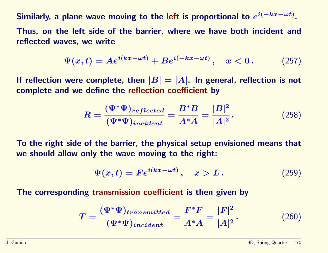
Similarly, a plane wave moving to the left is proportional to ei(−kx−ωt).

Thus, on the left side of the barrier, where we have both incident andreflected waves, we write

Ψ(x, t) = Aei(kx−ωt) +Bei(−kx−ωt) , x < 0 . (257)

If reflection were complete, then |B| = |A|. In general, reflection is notcomplete and we define the reflection coefficient by

R =(Ψ∗Ψ)reflected(Ψ∗Ψ)incident

=B∗B

A∗A=

|B|2

|A|2. (258)

To the right side of the barrier, the physical setup envisioned means thatwe should allow only the wave moving to the right:

Ψ(x, t) = Fei(kx−ωt) , x > L . (259)

The corresponding transmission coefficient is then given by

T =(Ψ∗Ψ)transmitted

(Ψ∗Ψ)incident=F ∗F

A∗A=

|F |2

|A|2. (260)


Since a given particle is either transmitted or reflected, these probabilitiesshould sum to unity:

R+ T = 1 (261)

is as sum rule that should emerge from the mathematics.

When the wave is in the barrier region itself, the SE takes a differentform.

d2ψ

dx2=

2m(U − E)

h2 ψ(x) ≡ α2ψ(x) , (262)

where we are considering the situation with U > E so that the α2 onthe rhs above is positive (as opposed to the negative −2mE

h2 that appliesoutside the barrier region). The solutions of this equation are exponentialdecay or increase. We should allow for both by writing

Ψ(x, t) = ψ(x)e−iωt = Ce−αx−iωt+De+αx−iωt 0 ≤ x ≤ L . (263)

Setting up the mathematics: boundary conditions

We employ continuity of Ψ and of ∂Ψ∂x

at the right and left sides of the


barrier to obtain:

A+B = C +D , (continuity of Ψ at x = 0)ikA− ikB = αD − αC , (continuity of ∂Ψ

∂xat x = 0)

Ce−αL +De+αL = FeikL , (continuity of Ψ at x = L)(αL)e+αL − (αC)e−αL = ikFeikL , (continuity of ∂Ψ

∂xat x = L)

(264)These equations can be solved. It takes a number of pages. Perhaps Iwill include the algebra in these notes at a later time. What one finds isthat

T (E) =1

1 + 14

[U2

E(U−E)

]sinh2αL

, E < U . (265)

And, we can check that the sum rule R + T = 1 is true. In the above,sinhx = (ex − e−x)/2. Note that for this case of E < U we findT (E) < 1 always. If E > U , the wave behavior in the barrier regionis oscillatory, and there will generally be a series of E values for whichT (E) = 1. These are called transmission resonances.

Example

Two wires are separated by an insulating layer. Modeling the latter as a


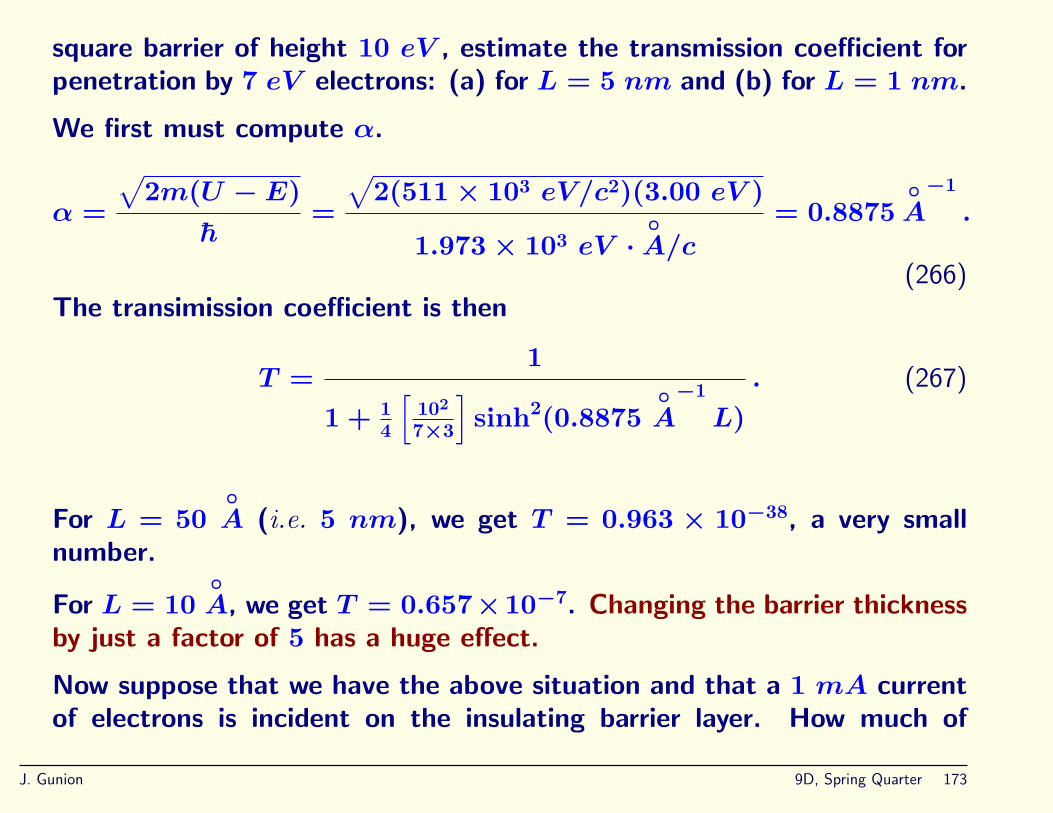
square barrier of height 10 eV , estimate the transmission coefficient forpenetration by 7 eV electrons: (a) for L = 5 nm and (b) for L = 1 nm.

We first must compute α.

α =

√2m(U − E)

h=

√2(511 × 103 eV/c2)(3.00 eV )

1.973 × 103 eV ·◦A/c

= 0.8875◦A

−1

.

(266)The transimission coefficient is then

T =1

1 + 14

[102

7×3

]sinh2(0.8875

◦A

−1

L). (267)

For L = 50◦A (i.e. 5 nm), we get T = 0.963 × 10−38, a very small

number.

For L = 10◦A, we get T = 0.657×10−7. Changing the barrier thickness

by just a factor of 5 has a huge effect.

Now suppose that we have the above situation and that a 1 mA currentof electrons is incident on the insulating barrier layer. How much of


this current passes through the layer to the adjacent wire if the electronenergies are 7 eV and the layer thickness is 1 nm.

Answer: Each of the e−’s in the current has the probability given byT = 0.657 × 10−7 to pass through the insulating layer. The cumulativeeffect will be a transmitted current of

T×1mA = 0.657×10−7×1mA = 0.657×10−7 mA = 6.57×10−11 A .(268)

Heisenberg Uncertainty Intuition

Another way to understand the tunneling phenomenon is to focus on themost important component of T (E), namely the exponential suppressionfactor for large L from the sinh function:

T (E) ∼ e−2αL × less important factors ∼ e−2L√

2m(U−E)/h ∼ e−2L/δ .(269)

Here, δ has the same meaning as in the finite well bound state situation;it is the length scale describing penetration of the wave into a forbiddne


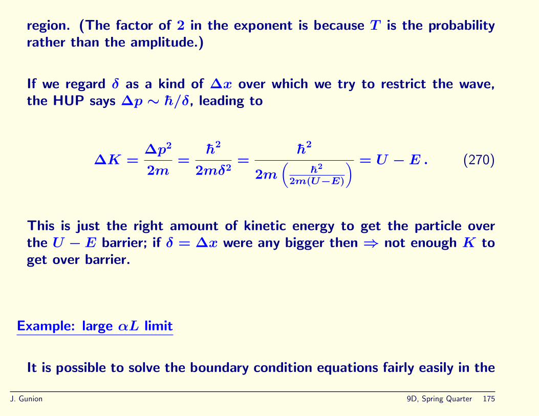
region. (The factor of 2 in the exponent is because T is the probabilityrather than the amplitude.)

If we regard δ as a kind of ∆x over which we try to restrict the wave,the HUP says ∆p ∼ h/δ, leading to

∆K =∆p2

2m=

h2

2mδ2=

h2

2m(

h2

2m(U−E)

) = U − E . (270)

This is just the right amount of kinetic energy to get the particle overthe U −E barrier; if δ = ∆x were any bigger then ⇒ not enough K toget over barrier.

Example: large αL limit

It is possible to solve the boundary condition equations fairly easily in the


case where e+αL is a big number. I repeat those equations here.

A+B = C +D , (continuity of Ψ at x = 0)ikA− ikB = αD − αC , (continuity of ∂Ψ

∂xat x = 0)

Ce−αL +De+αL = FeikL , (continuity of Ψ at x = L)(αL)e+αL − (αC)e−αL = ikFeikL , (continuity of ∂Ψ

∂xat x = L)

(271)If e+αL is large, then D (but not DeαL) must be small (from 3rd b.c.equation). The first two equations are then easily solved. Setting A = 1(A normalization just sets overall flux), we find very easily (multiply 1stequation by ik and add to 2nd equation to eliminate B terms) that

C =2ik

ik − α=

2

1 − αik

. (272)

If we define C′ ≡ Ce−αL and D′ ≡ De+αL, then the 3rd of the b.c.equations (271) + 1

ik× 4th b.c. equation yields

C′ +D′ =1

ik(−αC′ + αD′) , ⇒ D′ = C′

αik

+ 1αik

− 1


⇒

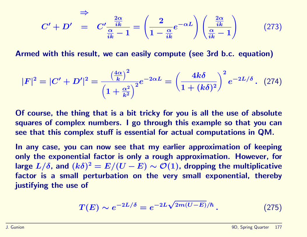
C′ +D′ = C′2αik

αik

− 1=

(2

1 − αik

e−αL

)(2αik

αik

− 1

)(273)

Armed with this result, we can easily compute (see 3rd b.c. equation)

|F |2 = |C′ +D′|2 =

(4αk

)2(1 + α2

k2

)2e−2αL =

(4kδ

1 + (kδ)2

)2

e−2L/δ . (274)

Of course, the thing that is a bit tricky for you is all the use of absolutesquares of complex numbers. I go through this example so that you cansee that this complex stuff is essential for actual computations in QM.

In any case, you can now see that my earlier approximation of keepingonly the exponential factor is only a rough approximation. However, forlarge L/δ, and (kδ)2 = E/(U −E) ∼ O(1), dropping the multiplicativefactor is a small perturbation on the very small exponential, therebyjustifying the use of

T (E) ∼ e−2L/δ = e−2L√

2m(U−E)/h . (275)


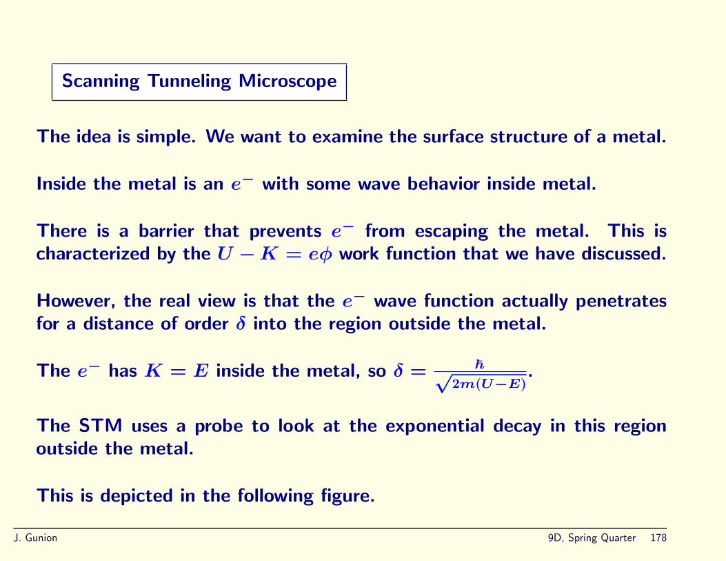
Scanning Tunneling Microscope

The idea is simple. We want to examine the surface structure of a metal.

Inside the metal is an e− with some wave behavior inside metal.

There is a barrier that prevents e− from escaping the metal. This ischaracterized by the U −K = eφ work function that we have discussed.

However, the real view is that the e− wave function actually penetratesfor a distance of order δ into the region outside the metal.

The e− has K = E inside the metal, so δ = h√2m(U−E)

.

The STM uses a probe to look at the exponential decay in this regionoutside the metal.

This is depicted in the following figure.


U=e

L

probe

exp[−x/ ]δ

ψ

ψ

φ + K

Figure 33: Scanning Tunneling Miscroscope setup. φ=work function. Ψ=wave function.

Typical numbers would be U = 9 eV and E = 5 eV , ⇒ U−E = 4 eV .


Then

δ =h√

2m(U − E)=

hc√2mc2(U − E)

=1.973 keV ·

◦A√

2(511 keV )(4 × 10−3 keV )' 1

◦A . (276)

A “bias” voltage V would be introduced between the metal surface andthe probe to ensure that the probe is probing the metal and not thereverse. The tunneling current would be given by

i =e2V

4π2Lδhe−2L/δ , (277)

and if L changes by even a small amount (i.e. if there is variation in thesurface defined by the e− wave functions), we will see a change in i.

In the above example, if L → L+ 0.01◦A then i changes by a fractional

amount of e−0.01×2/1◦A ' 0.98. Such a 2% change in i is measurable

using appropriate amplification techniques. Thus, one can have sensitivity

to surface details at the 0.01◦A level.


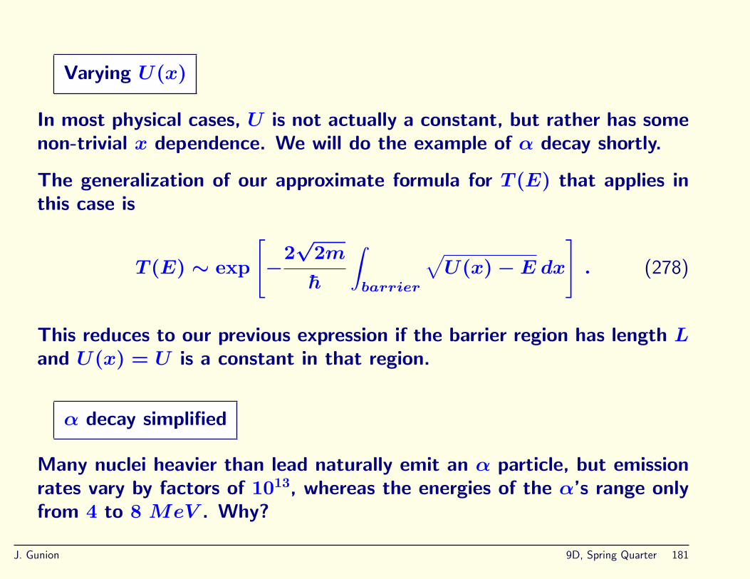
Varying U(x)

In most physical cases, U is not actually a constant, but rather has somenon-trivial x dependence. We will do the example of α decay shortly.

The generalization of our approximate formula for T (E) that applies inthis case is

T (E) ∼ exp

[−

2√

2m

h

∫barrier

√U(x) − E dx

]. (278)

This reduces to our previous expression if the barrier region has length Land U(x) = U is a constant in that region.

α decay simplified

Many nuclei heavier than lead naturally emit an α particle, but emissionrates vary by factors of 1013, whereas the energies of the α’s range onlyfrom 4 to 8 MeV . Why?


The basic picture is below.

Fig. 7−9, p.245

Figure 34: Picture of α decay.


Consider the α-particle emission of 238U (nuclear charge of 92) whichturns into an unstable isotope of Th by emitting a 4.2 MeV α particle,i.e. Eescape = 4.2 MeV .

We know that Rnucleus ∼ 7 × 10−15 m. This means that there is abarrier height at R coming from the Coulomb attraction that is of order(Z is the charge of the daughter nucleus in what follows))

Vcoulomb(R) =2kZe2

R

=2(90)(1.6 × 10−19 C)2(9 × 109 N ·m2/C2)

7 × 10−15 m

×10−6 MeV

1.6 × 10−19 J= 37 MeV . (279)

The α must tunnel through to radius

R1 =2kZe2

E=

2(9 × 109 N ·m2/C2)(90)(1.6 × 10−9 C)2

4.2 MeV

=37 MeV ×R

4.2 MeV= 6.2 × 10−14 m = 62 fm . (280)


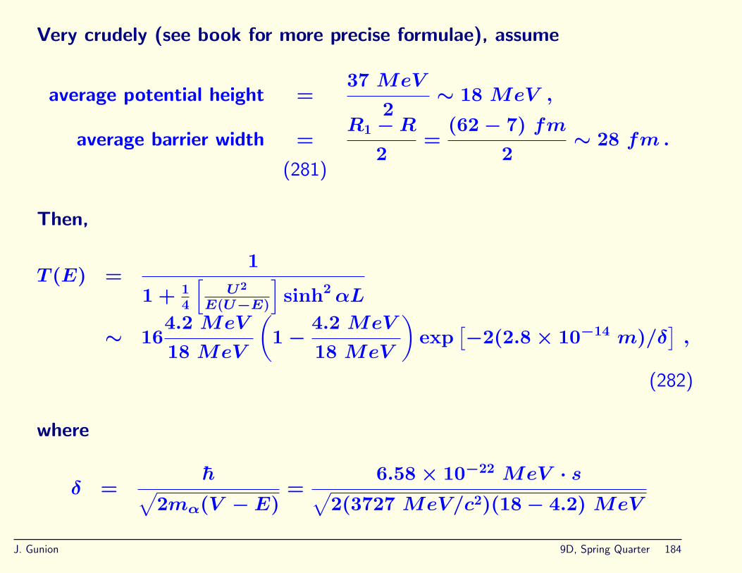
Very crudely (see book for more precise formulae), assume

average potential height =37 MeV

2∼ 18 MeV ,

average barrier width =R1 −R

2=

(62 − 7) fm

2∼ 28 fm .

(281)

Then,

T (E) =1

1 + 14

[U2

E(U−E)

]sinh2αL

∼ 164.2 MeV

18 MeV

(1 −

4.2 MeV

18 MeV

)exp

[−2(2.8 × 10−14 m)/δ

],

(282)

where

δ =h√

2mα(V − E)=

6.58 × 10−22 MeV · s√2(3727 MeV/c2)(18 − 4.2) MeV


= 6 × 10−16 m = 0.6 fm . (283)

This gives

e−2·28/0.6 = 2.9 × 10−41 , ⇒ T = 1.6 × 10−41 . (284)

So, you might say how can it ever escape?

The point is that the above is the probability for tunneling in a singlecollision of the α particle with the barrier. We must ask how manycollisions there are per second.

Inside the nucleus, the e− kinetic energy is roughly

K =1

2mv2 , ⇒

v =

√2K

m=

√2(4.2 MeV )

3727 MeV/c2= 0.047 c = 1.4 × 107 m/s ,(285)

where we should note that the output v implies that the NR approximationis ok.


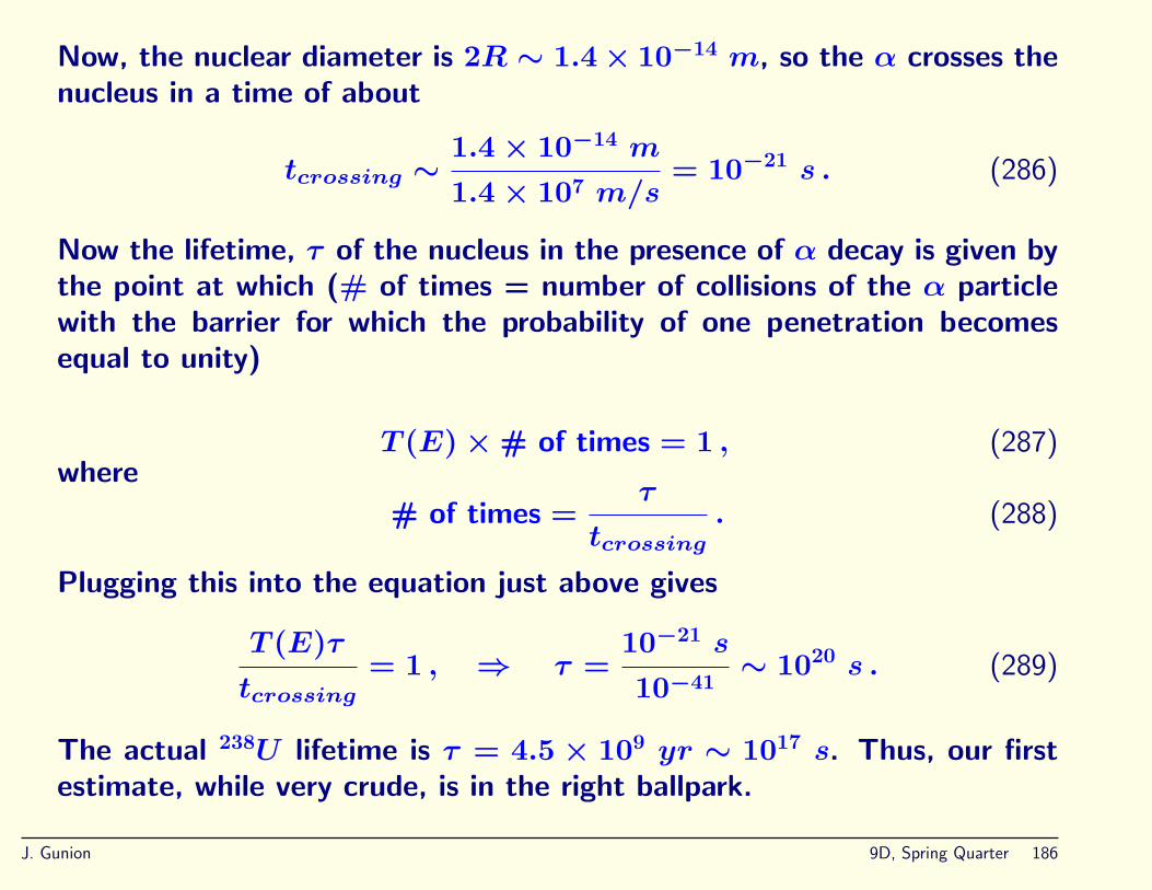
Now, the nuclear diameter is 2R ∼ 1.4 × 10−14 m, so the α crosses thenucleus in a time of about

tcrossing ∼1.4 × 10−14 m

1.4 × 107 m/s= 10−21 s . (286)

Now the lifetime, τ of the nucleus in the presence of α decay is given bythe point at which (# of times = number of collisions of the α particlewith the barrier for which the probability of one penetration becomesequal to unity)

T (E) × # of times = 1 , (287)where

# of times =τ

tcrossing. (288)

Plugging this into the equation just above gives

T (E)τ

tcrossing= 1 , ⇒ τ =

10−21 s

10−41∼ 1020 s . (289)

The actual 238U lifetime is τ = 4.5 × 109 yr ∼ 1017 s. Thus, our firstestimate, while very crude, is in the right ballpark.


To get a more precise result (in better agreement with experiment), onemust actually carry out the integral

T (E) ∼ exp

[−

2√

2m

h

∫barrier

√U(x) − E dx

]. (290)

using the potential drawn. This gives (to a good approximation)

T (E) = exp

−4πZ

√E0

E+ 8

√ZR

r0

, (291)

where r0 = h2

mαke2 is a kind of a Z = 1 Bohr radius for the α particle:r0 ∼ a0/7295 ∼ 7.25 fm since mα ∼ 7295me, and the associatedZ = 1 kinetic energy is

E0 =ke2

2r0=ke2

2a0

a0

r0= 13.6 eV × 7295 = 0.0993 MeV . (292)


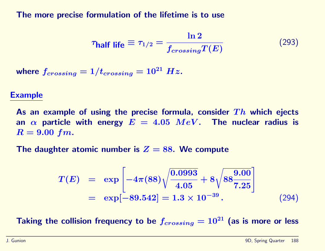
The more precise formulation of the lifetime is to use

τhalf life ≡ τ1/2 =ln 2

fcrossingT (E)(293)

where fcrossing = 1/tcrossing = 1021 Hz.

Example

As an example of using the precise formula, consider Th which ejectsan α particle with energy E = 4.05 MeV . The nuclear radius isR = 9.00 fm.

The daughter atomic number is Z = 88. We compute

T (E) = exp

[−4π(88)

√0.0993

4.05+ 8

√88

9.00

7.25

]= exp[−89.542] = 1.3 × 10−39 . (294)

Taking the collision frequency to be fcrossing = 1021 (as is more or less


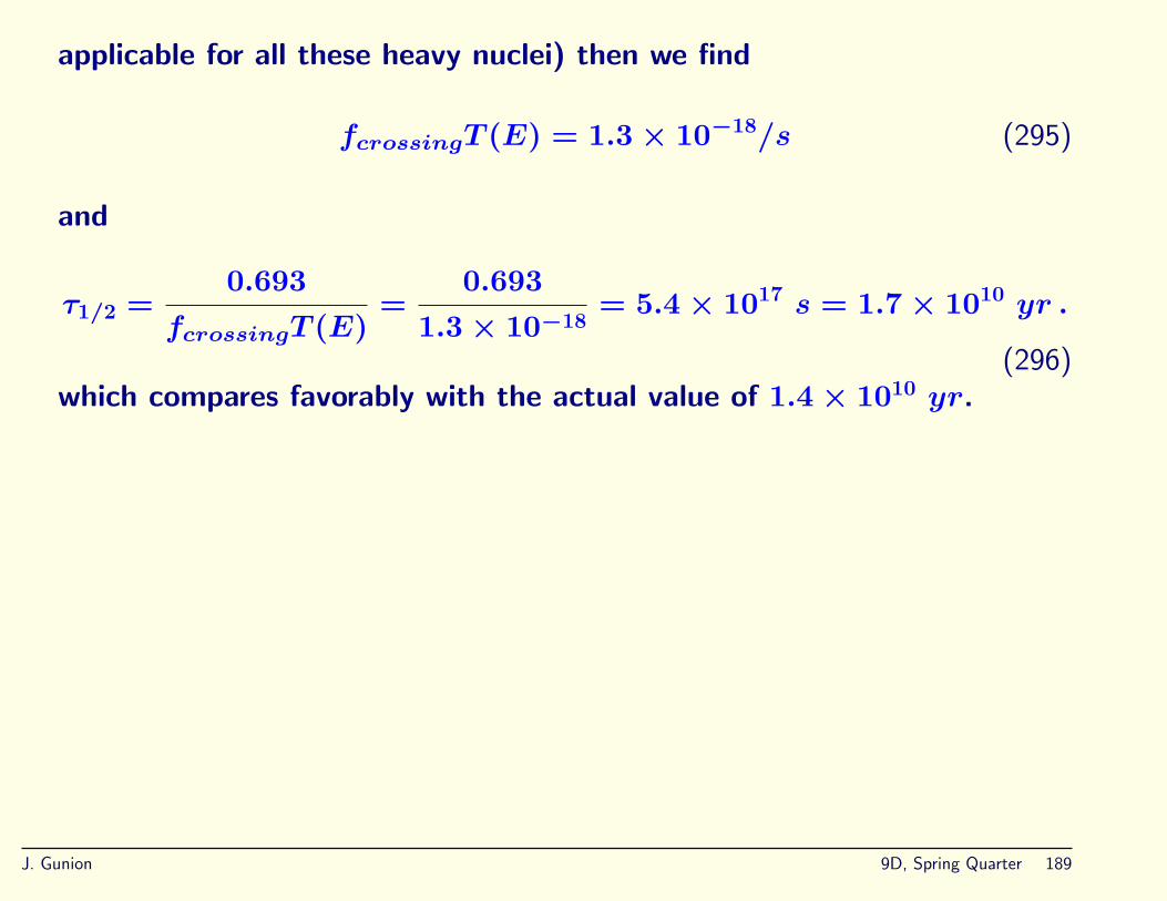
applicable for all these heavy nuclei) then we find

fcrossingT (E) = 1.3 × 10−18/s (295)

and

τ1/2 =0.693

fcrossingT (E)=

0.693

1.3 × 10−18= 5.4 × 1017 s = 1.7 × 1010 yr .

(296)which compares favorably with the actual value of 1.4 × 1010 yr.


Date post:	12-Jun-2018
Category:	Documents
Upload:	ngokhuong
View:	228 times
Download:	0 times

J. Gunion U.C. Davis 9D, Spring Quarterhiggs.physics.ucdavis.edu/9D_part2.pdfU.C. Davis 9D, Spring...

Documents