One-Shot Private Classical Capacity of Quantum Wiretap Channel: Based on one-shot quantum covering lemma Jaikumar Radhakrishnan * Pranab Sen † Naqueeb Ahmad Warsi ‡ Abstract In this work we study the problem of communication over the quantum wiretap channel. For this channel there are three parties Alice (sender), Bob (legitimate receiver) and Eve (eavesdropper). We obtain upper and lower bounds on the amount of information Alice can communicate to Bob such that Eve gets to know as little information as possible about the transmitted messages. Our bounds are in terms of quantum hypothesis testing divergence and smooth max quantum relative entropy. To obtain our result we prove a one-shot version of the quantum covering lemma along with operator Chernoff bound for non-square matrices. 1 lntroduction In this work we consider the problem of communication over a quantum wiretap channel with one sender (Alice) and two receivers (Bob and Eve). They have access to a channel that takes one input X (supplied by Alice) and produces two outputs Y and Z , received by Bob and Eve respectively. The characteristic of the channel is given by p YZ|X . The goal is to obtain bound on the amount of information Alice may can communicate to Bob such that Eve gets to know as little information as possible about the transmitted messages. Secrecy capacity of a sequence of wiretap channels in the information spectrum setting [1]: Bloch and Laneman studied the above problem in the classical asymptotic non-iid setting (information spectrum) wherein they defined various measures of secrecy [1]. One such secrecy measure is the L 1 distance kp MZ - p M × p Z k, where the distribution p MZ represents the joint distribution between the transmitted message random variable and the channel output at the Eve’s end when Alice transmits M . To place our contributions in place, it will be useful to revisit the result of Bloch and Laneman. But we need the following definitions to state Bloch and Laneman’s result. Definition 1. An (n, R, ε n ,δ n )-wiretap code for a sequence of wiretap channels p YZ|X consists of the fol- lowing: * Tata Institute of Fundamental Research, Mumbai, Email: [email protected]† Tata Institute of Fundamental Research, Mumbai, Email: [email protected]‡ SPMS, NTU, CQT, NUS, Singapore, IIITD, Delhi Email: [email protected]1 arXiv:1703.01932v1 [quant-ph] 6 Mar 2017
Transcript
One-Shot Private Classical Capacity of Quantum Wiretap Channel:Based on one-shot quantum covering lemma
Jaikumar Radhakrishnan ∗ Pranab Sen † Naqueeb Ahmad Warsi ‡
Abstract
In this work we study the problem of communication over the quantum wiretap channel. For thischannel there are three parties Alice (sender), Bob (legitimate receiver) and Eve (eavesdropper). We obtainupper and lower bounds on the amount of information Alice can communicate to Bob such that Eve gets toknow as little information as possible about the transmitted messages. Our bounds are in terms of quantumhypothesis testing divergence and smooth max quantum relative entropy. To obtain our result we provea one-shot version of the quantum covering lemma along with operator Chernoff bound for non-squarematrices.
1 lntroduction
In this work we consider the problem of communication over a quantum wiretap channel with one sender(Alice) and two receivers (Bob and Eve). They have access to a channel that takes one input X (suppliedby Alice) and produces two outputs Y and Z, received by Bob and Eve respectively. The characteristicof the channel is given by pY Z|X . The goal is to obtain bound on the amount of information Alice maycan communicate to Bob such that Eve gets to know as little information as possible about the transmittedmessages.
Secrecy capacity of a sequence of wiretap channels in the information spectrum setting [1]: Blochand Laneman studied the above problem in the classical asymptotic non-iid setting (information spectrum)wherein they defined various measures of secrecy [1]. One such secrecy measure is the L1 distance ‖pMZ −pM × pZ‖, where the distribution pMZ represents the joint distribution between the transmitted messagerandom variable and the channel output at the Eve’s end when Alice transmits M . To place our contributionsin place, it will be useful to revisit the result of Bloch and Laneman. But we need the following definitions tostate Bloch and Laneman’s result.
Definition 1. An (n,R, εn, δn)-wiretap code for a sequence of wiretap channels pY Z|X consists of the fol-lowing:
∗Tata Institute of Fundamental Research, Mumbai, Email: [email protected]†Tata Institute of Fundamental Research, Mumbai, Email: [email protected]‡SPMS, NTU, CQT, NUS, Singapore, IIITD, Delhi Email: [email protected]
1
arX
iv:1
703.
0193
2v1
[qu
ant-
ph]
6 M
ar 2
017
• a message setMn :={
1, · · · , 2nR}
;
• a stochastic encoding function en :Mn → X n;
• a decoding function dn : Yn →Mn.
The rate of the code is defined as 1n log |Mn|. Let M be the random variable denoting the uniform choice of
message i ∈ Mn, and Y n(Zn) be the random variable representing the legitimate receiver (eavesdropper)output corresponding to en(M). The average probability of error is defined as εn = Pr {dn(Y n) 6= M} andthe secrecy is measured in terms of ‖pMZ − pM × pZ‖ .
Definition 2. A rate R is achievable for a sequence of wiretap channels pY Z|X if there exists a sequence of(n,R, εn, δn)-wiretap code such that limn→∞ εn = 0 and limn→∞ δn = 0.
The supremum of all such achievable rates is called the private capacity of the sequence wiretap channelspY Z|X and we represent it by P .
Definition 3. (Specrtal inf-mutual information rate [2]) Let V = {V n}∞n=1 and Y = {Y n}∞n=1 be twosequences of random variables where for every n, V n ∈ Vn, Y n ∈ Yn and (V n, Y n) ∼ pV nY n . The spectralinf-mutual information I(V;Y) is defined as follows
I(V;Y) := sup
{β : lim
n→∞Pr
{1
nlog
pV nY n
pV npY n< β
}= 0
}.
The probability on the R.H.S. of the above equation is calculated with respect to the distribution pV nY n .
Definition 4. (Specrtal sup-mutual information rate [2]) Let V = {V n}∞n=1 and Z = {Zn}∞n=1 be twosequences of random variables where for every n, V n ∈ Vn, Zn ∈ Zn and (V n, Zn) ∼ pV nZn . The spectralsup-mutual information I(V;Z) is defined as follows
I(V;Z) := inf
{β : lim
n→∞Pr
{1
nlog
pV nZn
pV npZn> β
}= 0
}.
The probability on the R.H.S. of the above equation is calculated with respect to the distribution pV nZn .
We now state the result of Bloch and Laneman [1].
Theorem 1. [1] Let pY Z|X :={pY nZn|Xn
}∞n=1
represent a sequence of wiretap channels. The secrecycapacity (P ) for this sequence of channels is the following:
P = max(V ,X)
(I [V ;Y ]− I [V ;Z]
), (1)
where (V ,X) represents a sequence of pair of random variables {V n, Zn}∞n=1 .
A quantum version of the wiretap channel was studied by Devetak in [3] and Cai-Winter-Yeung in [4],where instead of pY Z|X , the channel is characterised by the map NA→BE : S(HA) → S(HBE). Theyshowed the following.
2
Theorem 2. The private classical capacity of a quantum channelNA→BE in the asymptotic iid setting is thefollowing:
limk→∞
1
kP (N⊗k),
where P (N ) is defined asP (N ) := max
ρ(I[V ;B]σ − I[V ;E]σ) ,
where all the information theoretic quantities are calculated with respect to the following state:
σV BE =∑v∈V
pV (v)|v〉〈v|V ⊗NA→BE(ρAv ).
2 Our Result
We consider the above problem in the quantum one-shot setting. A quantum wiretap channel takes a quantuminput ρA and produces two quantum outputs ρB and ρE , received by Bob and Eve respectively. The charac-teristics of the channel is given by NA→BE(ρA) = ρBE . A communication scheme over a quantum wiretapchannel is illustrated in Figure 1 .
ChannelAlice Encoder
Eve
Bob
ρAM∈{ 1,· · ·,2R}
TrBρBE
TrEρBE
NA→BE
ρBE
M
Figure 1: Private classical information transmission model over a quantum channel
We need the following definition to discuss our results.
Definition 5 (Encoding, Decoding, Error, Secrecy). A one-shot (R, ε, δ)-code for a quantum wiretap channelconsists of
• an encoding function F : [2R]→ S(HA), such that∥∥ρME − ρM ⊗ ρE∥∥ ≤ δ, (2)
where ρME , ρM and ρE are appropriate marginals of the state ρMBE = 12R
∑m∈[2R] |m〉〈m| ⊗
NA→BE(F (m)).
• decoding POVMs {T Bm : m ∈ [2R]} such that the average probability of error
1
2R
∑m∈[2R]
pe(m) ≤ ε, (3)
3
wherepe(m) = Tr
[(I− T Bm
)N (F (m))
](4)
is the probability of error when Alice uses this scheme to transmit the message m.
Definition 6. (Quantum hypothesis testing divergence [5]) Let ρV B :=∑
v∈V pV (v)|v〉〈v|U ⊗ ρBv be aclassical quantum state. For ε ∈ [0, 1) the hypothesis testing divergence between the systems V and B isdefined as follows:
Iε0 [V ;B] := sup0�Γ�I
Tr[ΓρV B]≥1−ε
− log Tr[Γ(ρV ⊗ ρB
)].
Definition 7. (Quantum smooth max Renyi divergence) Let ρV E :=∑
v∈V pV (v)|v〉〈v|V ⊗ ρEv be a classicalquantum state. For ε ∈ [0, 1) the smooth max Renyi divergence between the systems V and E is defined asfollows:
Iε∞[V ;E] := inf
{γ :∑v∈V
pV (v)Tr[{ρEv � 2γρE
}ρEv]≤ ε
},
where ρE = TrV[ρV E
]and
{ρEv � 2γρE
}is the projector onto the positive Eigen space of the operator
ρEv − 2γρE .
Theorem 3. (Achievability) Let NA→BE be a quantum wiretap channel. Let V be a random variable takingvalues in V and F : V → S(HA). Consider the state
ρV BE =∑v∈V
pV (v)|v〉〈v|V ⊗NA→BE (ρAv ) . (5)
For every ε ∈ (0, 1) and δ ∈ (0, 2) there exists an (R, ε, δ)-code for the quantum wiretap channelNA→BE if
R ≤ sup{V,F}
(Iε′
0 [V ;B]−max{
0, I δ∞[V ;E]})
+ log(ε′)
+ log(δ9)−O (log log(dim(HE))) (6)
where 18ε′ ≤ ε and δ is such that 144√δ ≤ δ. The information theoretic quantities mentioned in (6) are
calculated with respect to the state given in (5).
Theorem 4. (Converse) For a quantum wiretap channel NA→BE any (R, ε, δ)-code satisfies the following:
R ≤ sup{V,F}
(Iε0 [V ;B]− Iδ∞ [V ;E]
)+ 1.5, (7)
where V is a random variable over a set V , F : V → S(HA) a map from V to S(HA) and all the informationtheoretic quantities are calculated with respect to the following state:
ΘV BE :=∑v∈V
p(v)|v〉〈v|V ⊗NA→BE (ρAv ) .
4
Techniques: Our achievability proof follows along the line of the proof in [6]. As before, we generate arow array, whose entries are generated according to the distribution pV ; furthermore, as in the original proofwe partition this array into bands of appropriate sizes and uniquely assign each of these bands to a message.To send a message m ∈ [2R], Alice chooses a codeword v uniformly from the band corresponding to m;applies the map F to v and then transmits the resulting state ρAv over the channel. Bob on receiving hisshare of the channel output tries to determine the codeword v using standard one-shot decoding techniquesfor a point to point quantum channel. He succeeds with high probability for the given codebook size. It onlyremains to show that the message m is secret from Eve. The random choice of v from the band correspondingto m should make Eve’s share of the channel output independent of m. This is the main technical hurdlethat must be overcome in order to prove the correctness of a code for a wiretap channel. In the asymptoticiid setting, this hurdle is overcome by proving a quantum covering lemma [6, Lemma 16.2.1] based on anoperator Chernoff bound of Ahlswede-Winter [7] for Hermitian matrices . Unfortunately, a straightforwardtranslation of this technique to one-shot setting fails. In this work, we overcome these difficulties and manageto prove for the first time a one-shot quantum covering lemma. On the way, we also prove a novel operatorChernoff bound for non-square matrices.
The proof for the converse (Theorem 4) essentially follows along the line of the proof given in [1]; thetranslation to the one-shot quantum setting is straightforward.
Private classical capacity of the quantum wiretap channel in the quantum information spectrum set-ting. Our bounds allow us to obtain the quantum version of Theorem 1. The quantum information spectrumtechnique pioneered by Hayashi and Nagaoka [8] allows one to derive meaningful bounds on rates even in theabsence of the iid assumption; however, the analysis is often more challenging in this setting. The bounds inour work are expressed using smooth min and max Renyi divergences. The close relationship between thesequantities and the quantities that typically arise in the information spectrum setting (see Datta and Leditzky[9]) allows us to derive the quantum version of Theorem 1.
Related work: In [10] Renes and Renner derive one-shot achievability and converse bounds for the quan-tum wiretap channel in terms of conditional min and max Renyi entropies. They also show that their resultasymptotically yields the results of [3] and [4]. However, the result of Renes and Renner [10] does not seemto yield the asymptotic characterisation of the wiretap channel in the information spectrum (non-iid) setting.Such a result as mentioned earlier in Theorem 1 is known for the classical case. We note here that our one-shotbounds which are stated in terms of two fundamental smooth Renyi divergences allow us to characterise thecapacity of the wiretap channel in the information spectrum (asymptotic non-iid) setting; our characterisationturns out to be nothing but the quantum analogue of the characterisation of Theorem 1.
3 Proof of Theorem 3
Proof. Let ρV B :=∑
v∈V pV (v)|v〉〈v|V ⊗ ρBv denote the joint state of the system V B, where ρBv :=TrE
[ρBEv
]. Also, let ρB := EV
[ρBV]. Let 0 � ΓV B � I satisfy the following properties
(P1) Tr[ΓV BρV B
]> 1− ε′.
(P2) Iε′
0 [V ;B] = − log Tr[ΓV B
(ρV ⊗ ρB
)].
5
See Definition 6 for the definition of Iε′
0 [V ;B]. Fix R such that
R ≤ Iε′0 [V ;B]−max{
0, I δ∞[V ;E]}
+ log(ε′)− log
(1016 (log dim(HE))6
δ9
(− ln
(δ
30C
))),
where C = dim(HE)(
log2
(4 dim(HE)
δ
)+ 1)2
. Furthermore, let R be such that
R = max{
0, I δ∞[V ;E]}
+ log
(1016 (log dim(HE))6
δ9
(− ln
(δ
30C
))). (8)
See Definition ?? for the definition of I δ∞[V ;E].
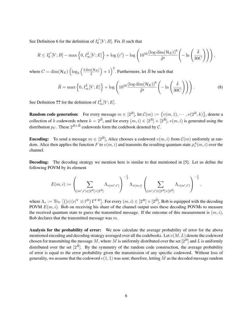
Random code generation: For every message m ∈ [2R], let C(m) :={v(m, 1), · · · , v(2R, k)
}, denote a
collection of k codewords where k = 2R, and for every (m, i) ∈ [2R] × [2R], v(m, i) is generated using thedistribution pV . These 2R+R codewords form the codebook denoted by C.
Encoding: To send a message m ∈ [2R], Alice chooses a codeword v(m, i) from C(m) uniformly at ran-dom. Alice then applies the function F to v(m, i) and transmits the resulting quantum state ρAv (m, i) over thechannel.
Decoding: The decoding strategy we mention here is similar to that mentioned in [5]. Let us define thefollowing POVM by its element
E(m, i) :=
∑(m′,i′)∈[2R]×[2R]
Λv(m′,i′)
− 12
Λv(m,i)
∑(m′,i′)∈[2R]×[2R]
Λv(m′,i′)
− 12
,
where Λv := TrV[(|v〉〈v|V ⊗ IB
)ΓV B
]. For every (m, i) ∈ [2R]× [2R], Bob is equipped with the decoding
POVM E(m, i). Bob on receiving his share of the channel output uses these decoding POVMs to measurethe received quantum state to guess the transmitted message. If the outcome of this measurement is (m, i),Bob declares that the transmitted message was m.
Analysis for the probability of error: We now calculate the average probability of error for the abovementioned encoding and decoding strategy averaged over all the codebooks. Let v(M,L) denote the codewordchosen for transmitting the messageM , whereM is uniformly distributed over the set [2R] and L is uniformlydistributed over the set [2R]. By the symmetry of the random code construction, the average probabilityof error is equal to the error probability given the transmission of any specific codeword. Without loss ofgenerality, we assume that the codeword v(1, 1) was sent; therefore, letting M as the decoded message random
6
variable, we have
EV[Pr{M 6= 1}
]≤ EV Tr
[(I− E(1, 1)) ρV (1,1)
]a≤ 2EV Tr
[(I− ΛV (1,1))ρV (1,1)
]+ 4
∑(m,i)6=(1,1)
EV Tr[ΛV (m,i)ρV (1,1)
]b= 2
(1− Tr
[ΓV BρV B
])+ 4
∑(m,i)6=(1,1)
Tr[ΓV B
(ρV ⊗ ρB
)]c≤ 2ε′ + 22+R+R−Iε′0 [V ;B]
d≤ 6ε′ (9)
where a follows from Hayashi Nagaoka operator inequality; b follows from the definition of ΛV ; c followsfrom the definition of ΓV B and d follows from our choice of R and R.
Analysis for the leaked information to Eve: Let ρME :=∑
m∈[2R]1
2R|m〉〈m| ⊗ ρEm be the joint state of
the system ME. Notice that in the setting of the problem for every m ∈ [2R]
ρEm =1
2R
∑l∈[1:2R]
ρEv(m,l), (10)
where ρEv := TrB[ρBEv
]and ρBEv := NA→BE(ρAv ). Furthermore, let ρE = 1
2R
∑2R
m=1 ρEm and ρE :=
EV[ρEV]. The leakage information is now calculated as follows:∥∥∥∥∥∥
2R∑m=1
1
2R(|m〉〈m| ⊗ ρEm
)−
2R∑m=1
1
2R|m〉〈m| ⊗ ρE
∥∥∥∥∥∥ ≤2R∑m=1
1
2R∥∥ρEm − ρE∥∥ ,
≤2R∑m=1
1
2R∥∥ρEm − ρE∥∥+
∥∥ρE − ρE∥∥≤ 2
2R∑m=1
1
2R∥∥ρEm − ρE∥∥ ,
where all the above inequalities follow from the triangle inequality. Therefore, by the symmetry of the randomcode construction, we have
EC
∥∥∥∥∥∥2R∑m=1
1
2R(|m〉〈m| ⊗ ρEm
)−
2R∑m=1
1
2R|m〉〈m| ⊗ ρE
∥∥∥∥∥∥ ≤ 2
2R∑m=1
1
2REC∥∥ρEm − ρE∥∥ ,
= 2EC(1)
∥∥∥∥∥∥ 1
2R
∑l∈[1:2R]
ρEV (1,l) − ρE
∥∥∥∥∥∥ .
7
Thus, we can now conclude from Theorem 5 (see Section 6) with ε ← δ and I ← max{
0, I δ∞ [V ;E]}
, that
for our choice of R (see (8)) we have
EC
∥∥∥∥∥∥2R∑m=1
1
2R(|m〉〈m| ⊗ ρEm
)−
2R∑m=1
1
2R|m〉〈m| ⊗ ρE
∥∥∥∥∥∥ ≤ 48√δ.
Expurgation: Let ε(C) be a random variable representing the average probability of error where the ran-domization is over the random choice of the codebook C and let δ(C) be a random variable representing theleakage information and again the randomization is over the random choice of the codebook C. Further , wedefine the following events:
E1 :={ε(C) < 3EC Pr
{M 6= M
}}E2 :=
δ(C) < 3EC
∥∥∥∥∥∥2R∑m=1
1
2R(|m〉〈m| ⊗ ρEm
)−
2R∑m=1
1
2R|m〉〈m| ⊗ ρE
∥∥∥∥∥∥ .
Using Markov inequality it is easy to see from the definition of E1 and E2 that
Pr {E1, E2} >1
3.
Thus, we can now conclude that if R satisfies the condition of the theorem then there exists an (R, ε, δ)-codefor the quantum wiretap channel.
4 Proof of Theorem 4
We need the following key lemma which can be considered as the quantum generalization of [11, eq. 2.3.18,p.18].
Lemma 1. Let ρ and σ be two quantum states. Furthermore, let Π := {ρ � 2βσ} where β > 0 is arbitrary.Then,
||ρ− σ|| ≥ 2β ln 2
β ln 2 + 1Tr[Πρ]. (11)
Proof. The proof follows the fact that ‖ρ− σ‖ ≥ 2Tr [Π(ρ− σ)], [6, Lemma 9.1.1]. The claim now followsfrom the following set of inequlities,
‖ρ− σ‖ ≥ 2Tr [Π(ρ− σ)]a≥ 2Tr [Πρ]
(1− e−β ln 2
)b≥ 2Tr [Πρ]
(1− 1
1 + β ln 2
)=
2β ln 2
β ln 2 + 1Tr [Πρ] ,
where a follows because ΠρΠ � 2βΠσΠ and b follows because eβ ln 2 ≥ (1 + β ln 2). This completes theproof.
8
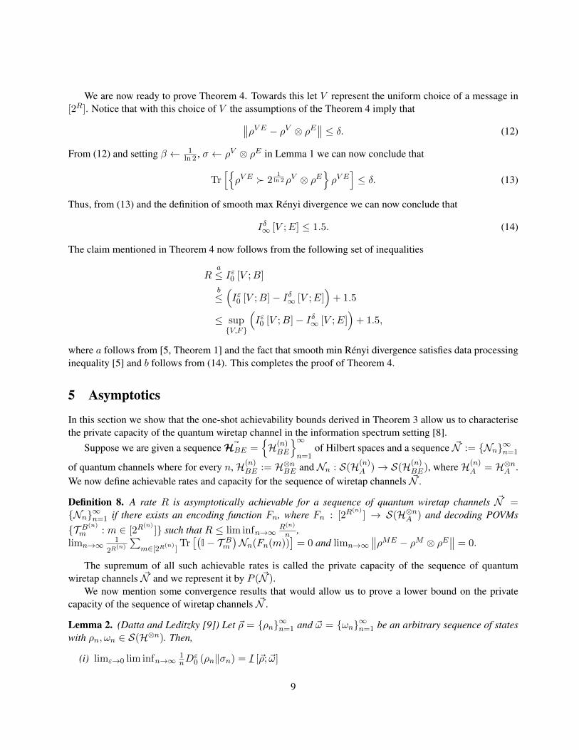
We are now ready to prove Theorem 4. Towards this let V represent the uniform choice of a message in[2R]. Notice that with this choice of V the assumptions of the Theorem 4 imply that∥∥ρV E − ρV ⊗ ρE∥∥ ≤ δ. (12)
From (12) and setting β ← 1ln 2 , σ ← ρV ⊗ ρE in Lemma 1 we can now conclude that
Tr[{ρV E � 2
1ln 2 ρV ⊗ ρE
}ρV E
]≤ δ. (13)
Thus, from (13) and the definition of smooth max Renyi divergence we can now conclude that
Iδ∞ [V ;E] ≤ 1.5. (14)
The claim mentioned in Theorem 4 now follows from the following set of inequalities
Ra≤ Iε0 [V ;B]
b≤(Iε0 [V ;B]− Iδ∞ [V ;E]
)+ 1.5
≤ sup{V,F}
(Iε0 [V ;B]− Iδ∞ [V ;E]
)+ 1.5,
where a follows from [5, Theorem 1] and the fact that smooth min Renyi divergence satisfies data processinginequality [5] and b follows from (14). This completes the proof of Theorem 4.
5 Asymptotics
In this section we show that the one-shot achievability bounds derived in Theorem 3 allow us to characterisethe private capacity of the quantum wiretap channel in the information spectrum setting [8].
Suppose we are given a sequence ~HBE ={H(n)BE
}∞n=1
of Hilbert spaces and a sequence ~N := {Nn}∞n=1
of quantum channels where for every n, H(n)BE := H⊗nBE and Nn : S(H(n)
A )→ S(H(n)BE), whereH(n)
A = H⊗nA .We now define achievable rates and capacity for the sequence of wiretap channels ~N .
Definition 8. A rate R is asymptotically achievable for a sequence of quantum wiretap channels ~N ={Nn}∞n=1 if there exists an encoding function Fn, where Fn : [2R
(n)] → S(H⊗nA ) and decoding POVMs
{T B(n)
m : m ∈ [2R(n)
]} such that R ≤ lim infn→∞R(n)
n ,limn→∞
1
2R(n)
∑m∈[2R
(n)]Tr[(
I− T Bm)Nn(Fn(m))
]= 0 and limn→∞
∥∥ρME − ρM ⊗ ρE∥∥ = 0.
The supremum of all such achievable rates is called the private capacity of the sequence of quantumwiretap channels ~N and we represent it by P ( ~N ).
We now mention some convergence results that would allow us to prove a lower bound on the privatecapacity of the sequence of wiretap channels ~N .
Lemma 2. (Datta and Leditzky [9]) Let ~ρ = {ρn}∞n=1 and ~ω = {ωn}∞n=1 be an arbitrary sequence of stateswith ρn, ωn ∈ S(H⊗n). Then,
(i) limε→0 lim infn→∞1nD
ε0 (ρn‖σn) = I [~ρ; ~ω]
9
(ii) limε→0 lim supn→∞1nD
ε∞ (ρn‖σn) = I [~ρ; ~ω]
An immediate consequence of the Theorem 3, Definition 8 and Lemma 2 is the following corollary.
Corollary 1. The private capacity P ( ~N ) of the sequence of quantum wiretap channels ~N satisfies the fol-lowing lower bounds
P ( ~N ) ≥ sup{V n,Fn}∞n=1
(I[V;B]− I[V;E]
),
where for every n, the random variable V n takes values over the set Vn, Fn : Vn → S(H⊗nA ) and all the in-formation theoretic quantities are calculated with respect to the sequence of state ~ΘV BE :=
{ΘV nBnEn}∞
n=1,
where for every nΘV nBnEn
:=∑vn∈Vn
p(vn)|vn〉〈vn|V n ⊗NAn→Bn
n
(ρA
n
vn).
Furthermore, using steps exactly similar to that used in the proof of Theorem 4 we can prove the followingcorollary.
Corollary 2. The private capacity P ( ~N ) of the sequence of quantum wiretap channels ~N satisfies the fol-lowing upper bounds
P ( ~N ) ≤ sup{V n,Fn}∞n=1
(I[V;B]− I[V;E]
),
where for every n, the random variable V n takes values over the set Vn, Fn : Vn → S(H⊗nA ) and all the in-formation theoretic quantities are calculated with respect to the sequence of state ~ΘV BE :=
{ΘV nBnEn}∞
n=1,
where for every nΘV nBnEn
:=∑vn∈Vn
p(vn)|vn〉〈vn|V n ⊗NAn→Bn
n
(ρA
n
vn).
Proof. Let the rate R be achievable. Therefore, there exists a sequence of codes satisfying the conditionsmentioned in Definition 8. Furthermore, let V n be uniformly distributed over [2nR]. Notice that for thischoice of V n the conditions mentioned in Definition 8 imply that
I[V ;E] = 0. (15)
The claim now follows from the following set of inequalities
Ra≤ I[V;B]
b= I[V;B]− I[V;E]
≤ max{Vn,Fn}∞n=1
(I[V;B]− I[V;E]
),
where a follows from [8, Lemma 3] and b follows from (15). This completes the proof.
Thus, an immediate consequence of Corollary 1 and Corollary 2 is the following proposition.
10
Proposition 1. The private capacity P ( ~N ) of the sequence of quantum wiretap channels ~N satisfies thefollowing
P ( ~N ) = sup{V n,Fn}∞n=1
(I[V;B]− I[V;E]
),
where for every n, the random variable V n takes values over the set Vn, Fn : Vn → S(H⊗nA ) and all the infor-mation theoretic quantities are calculated with respect to the sequence of states ~ΘV BE :=
{ΘV nBnEn}∞
n=1,
where for every nΘV nBnEn
:=∑vn∈Vn
p(vn)|vn〉〈vn|V n ⊗NAn→Bn
n
(ρA
n
vn).
6 One-Shot Quantum Covering Lemma
Theorem 5. Let X be a random variable taking values in the set X . For each x ∈ X , let ρx be a quantumstate in the space H. Let ρ = EX[ρX] be the average of the the states ρx. Fix I ≥ 0, and for each x ∈ Xdefine (based on I) the projection Πx and real number εx ∈ (0, 1) as follows:
Πx = {2Iρ � ρx};εx = 1− Tr [Πxρx] .
Let ε = EX[εX]. Suppose s = (X[1],X[2], . . . ,X[M ]) is a sequence of independent random samples drawnaccording to the distribution of X, and let ρ = Em∈[M ][ρX[m]]. Then,
Prs
{‖ρ− ρ‖ ≥ 22
√ε}≤ 30C exp
(− 10−16ε9
(log2 (dim(H)))6
M
2I
),
where C = dim(H)(
log2
(4 dim(H)
ε
)+ 1)2
.
Outline: To prove this concentration result, we will crucially employ the Operator Chernoff Bound ofAhlswede and Winter [7]. We will, however, need to partition the underlying space so that the operatorsinvolved are suitable for an application of the Operator Chernoff Bound. The operator Chernoff bound re-quires a lower bound on the the smallest Eigen value of the expectation operator. Hence, we have to partitionthe space into subspaces such that the ratio of the maximum Eigen value to the minimum Eigen value ofexpectation operator is not too large. We still have to take care of the very small Eigen values of expecta-tion operator but it turns out that we can simply neglect them introducing only small errors in the process.This strategy of partitioning the space breaks up the operators into blocks. The operator Chernoff bound candirectly be applied to the diagonal blocks. However, the off diagonal blocks pose a problem because theyare non-Hermitian matrices and non-square matrices and the operator Chernoff bound does not directly applyto them. We handle the off-diagonal blocks separately by proving a new Chernoff bound in terms of theSchatten-infinity norm. We believe the new Chernoff lemma will be of independent interest.
First, we present the tools we will need.
11
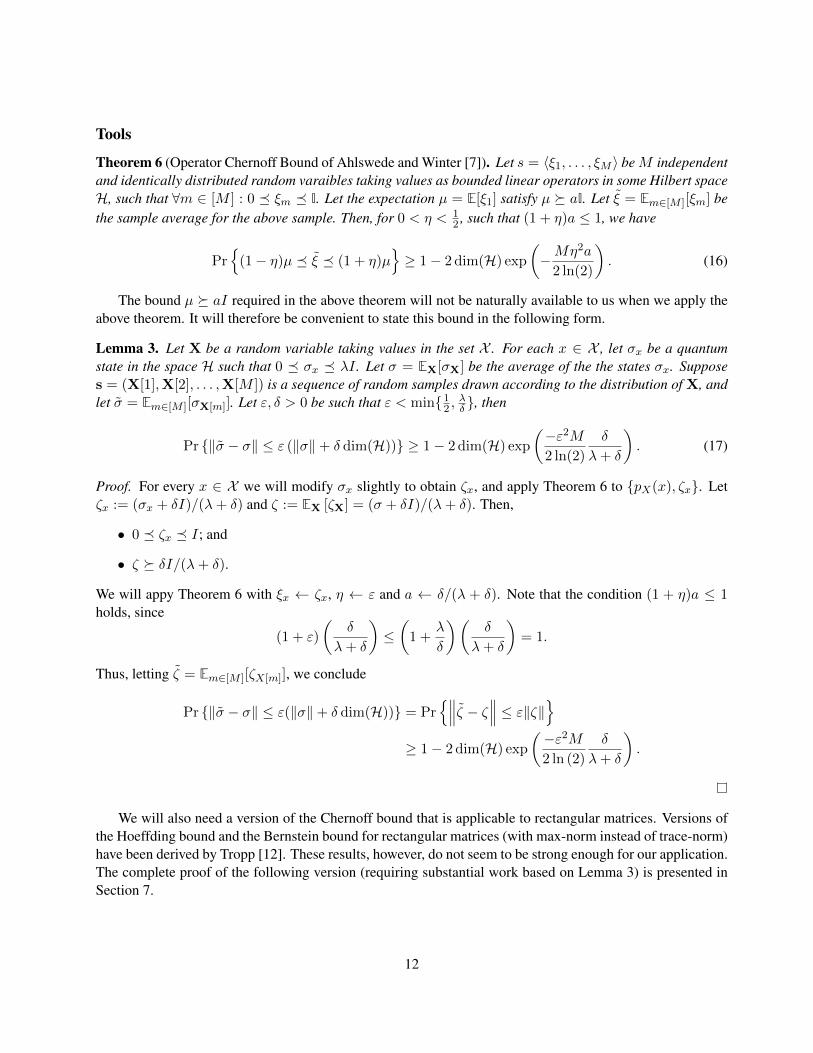
Tools
Theorem 6 (Operator Chernoff Bound of Ahlswede and Winter [7]). Let s = 〈ξ1, . . . , ξM 〉 beM independentand identically distributed random varaibles taking values as bounded linear operators in some Hilbert spaceH, such that ∀m ∈ [M ] : 0 � ξm � I. Let the expectation µ = E[ξ1] satisfy µ � aI. Let ξ = Em∈[M ][ξm] bethe sample average for the above sample. Then, for 0 < η < 1
2 , such that (1 + η)a ≤ 1, we have
Pr{
(1− η)µ � ξ � (1 + η)µ}≥ 1− 2 dim(H) exp
(−Mη2a
2 ln(2)
). (16)
The bound µ � aI required in the above theorem will not be naturally available to us when we apply theabove theorem. It will therefore be convenient to state this bound in the following form.
Lemma 3. Let X be a random variable taking values in the set X . For each x ∈ X , let σx be a quantumstate in the space H such that 0 � σx � λI . Let σ = EX[σX] be the average of the the states σx. Supposes = (X[1],X[2], . . . ,X[M ]) is a sequence of random samples drawn according to the distribution of X, andlet σ = Em∈[M ][σX[m]]. Let ε, δ > 0 be such that ε < min{1
Proof. For every x ∈ X we will modify σx slightly to obtain ζx, and apply Theorem 6 to {pX(x), ζx}. Letζx := (σx + δI)/(λ+ δ) and ζ := EX [ζX] = (σ + δI)/(λ+ δ). Then,
• 0 � ζx � I; and
• ζ � δI/(λ+ δ).
We will appy Theorem 6 with ξx ← ζx, η ← ε and a ← δ/(λ + δ). Note that the condition (1 + η)a ≤ 1holds, since
We will also need a version of the Chernoff bound that is applicable to rectangular matrices. Versions ofthe Hoeffding bound and the Bernstein bound for rectangular matrices (with max-norm instead of trace-norm)have been derived by Tropp [12]. These results, however, do not seem to be strong enough for our application.The complete proof of the following version (requiring substantial work based on Lemma 3) is presented inSection 7.
12
Lemma 4. Let X be a random variable taking values in the set X . Let d1 ≥ d2, β ≥ 1, and for each x ∈ X ,let Ax ∈ Cd1×d2 such that ‖Ax‖ ≤ 1 and ‖Ax‖∞ ≤ β
d2. Let A = EX[AX] be the average of the states Ax.
Suppose s = (X[1],X[2], . . . ,X[m]) is a sequence of random samples drawn according to the distributionof X , and let A = Em∈[M ][AX[m]]. Then, for 0 < ε < 1,
Prs
{‖A−A‖ ≥ ε
}≤ 25d1 exp
(−10−11ε3M
β
).
We will need the Gentle Measurement Lemma of Winter [13, Lemma 9] (see also [6, Lemma 9.4.2]).
Lemma 5. Let (px, ρx) be an ensemble of quantum states and ρ =∑
x pxρx. Let 0 � Λ � I and ε ∈ [0, 1]be such that Tr[Λρ] ≥ 1− ε. Then, ∑
x
px
∥∥∥ρx −√Λρx√
Λ∥∥∥ ≤ 2
√ε.
In particular, if Λ is a projection operator, then∑x
px ‖ρx − ΛρxΛ‖ ≤ 2√ε.
6.1 Proof of Theorem 5
As stated above, our proof will be obtained by decomposing the space. We first present this decomposition.
Decomposition of the space: We describe the decomposition by explicitly presenting the orthogonal pro-jector Πi onto the i-th component. LetD = dimH, and let the spectral decomposition of ρ be
∑Dj=1 λj |j〉〈j|,
where 1 ≥ λ1 ≥ λ2 ≥ · · · ≥ λD ≥ 0 and∑D
j=1 λj = 1. Then, for i = 1, 2, . . ., let
Πi =∑
j:2−(i−1)≥λj>2−i
|j〉〈j|.
Let K =⌈log2
(4 dim(H)
ε
)⌉, let Π? =
∑Ki=1 Πi and Πc
? =∑
i>K Πi; then
Tr [Πc?ρ] ≤ ε
4. (18)
Thus, intuitively, most of the mass of ρ resides in the subspace Π?. Hence, from triangle inequality and fromLemma 5 it now follows that to prove Theorem 5 it is sufficient to show that ‖ρ−Π?ρΠ?‖ is small enough.
Proof. We will be use the following abbreviations.
ρ′x := ΠxρxΠx
ρ′ := EX[ρ′X]
ρ := Em∈[M ][ρX[m]]
ρ′ := Em∈[M ][ρ′X[m]].
13
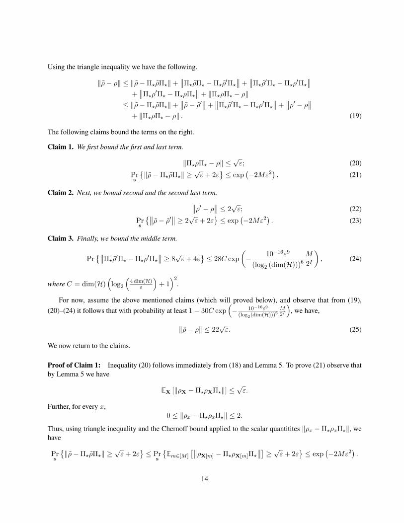
Using the triangle inequality we have the following.
‖ρ− ρ‖ ≤ ‖ρ−Π?ρΠ?‖+∥∥Π?ρΠ? −Π?ρ
′Π?
∥∥+∥∥Π?ρ
′Π? −Π?ρ′Π?
∥∥+∥∥Π?ρ
′Π? −Π?ρΠ?
∥∥+ ‖Π?ρΠ? − ρ‖≤ ‖ρ−Π?ρΠ?‖+
∥∥ρ− ρ′∥∥+∥∥Π?ρ
′Π? −Π?ρ′Π?
∥∥+∥∥ρ′ − ρ∥∥
+ ‖Π?ρΠ? − ρ‖ . (19)
The following claims bound the terms on the right.
Claim 1. We first bound the first and last term.
‖Π?ρΠ? − ρ‖ ≤√ε; (20)
Prs
{‖ρ−Π?ρΠ?‖ ≥
√ε+ 2ε
}≤ exp
(−2Mε2
). (21)
Claim 2. Next, we bound second and the second last term.∥∥ρ′ − ρ∥∥ ≤ 2√ε; (22)
Prs
{∥∥ρ− ρ′∥∥ ≥ 2√ε+ 2ε
}≤ exp
(−2Mε2
). (23)
Claim 3. Finally, we bound the middle term.
Pr{∥∥Π?ρ
′Π? −Π?ρ′Π?
∥∥ ≥ 8√ε+ 4ε
}≤ 28C exp
(− 10−16ε9
(log2 (dim(H)))6
M
2I
), (24)
where C = dim(H)(
log2
(4 dim(H)
ε
)+ 1)2
.
For now, assume the above mentioned claims (which will proved below), and observe that from (19),(20)–(24) it follows that with probability at least 1− 30C exp
(− 10−16ε9
(log2(dim(H)))6M2I
), we have,
‖ρ− ρ‖ ≤ 22√ε. (25)
We now return to the claims.
Proof of Claim 1: Inequality (20) follows immediately from (18) and Lemma 5. To prove (21) observe thatby Lemma 5 we have
EX [‖ρX −Π?ρXΠ?‖] ≤√ε.
Further, for every x,0 ≤ ‖ρx −Π?ρxΠ?‖ ≤ 2.
Thus, using triangle inequality and the Chernoff bound applied to the scalar quantitites ‖ρx −Π?ρxΠ?‖, wehave
Prs
{‖ρ−Π?ρΠ?‖ ≥
√ε+ 2ε
}≤ Pr
s
{Em∈[M ]
[∥∥ρX[m] −Π?ρX[m]Π?
∥∥] ≥ √ε+ 2ε}≤ exp
(−2Mε2
).
14
Proof of Claim 2: From our assumption, ε = EX [εX ] = 1−EX[Tr ΠXρX]; that is, EX[Tr ΠXρX] = 1−ε.Using the triangle inequality, Lemma 5 and Jensen’s inequality, we derive (22) as follows:
‖ρ′ − ρ‖ ≤ EX
[‖ρ′X − ρX‖
]≤ EX [2
√εX] ≤ 2
√ε.
Now (23) follows by applying the Chernoff bound to the scalar quantities ‖ρ′x − ρx‖.
Proof of Claim 3: This claim will need substantial work. Both expressions Π?ρ′Π? and Π?ρ
′Π? involve theoperators ρ′x = ΠxρxΠx. The first expression is the expectation of ρ?,x := Π?ρ
′xΠ? over the samples, whereas
the the second expression is the expectation of ρ?,x under the original distribution. That these quantities withhigh probability should be close to each other would intuitively follow from the Operator Chernoff Bound.However, we need to prepare the operators for an application of the bound. In fact, for every x ∈ X we willobtain a decomposition
ρ?,x = ρ−?,x + ρ+?,x, (26)
(ρ−?,x and ρ+?,x are orthogonal) such that
EX
[Tr[ρ+
?,X]]≤ 4ε, (27)
implying (by Lemma 5)EX[∥∥∥ρ?,X − ρ−?,X∥∥∥] ≤ 4
√ε, (28)
from which by a routine application Chernoff bound to the scalar quantitites∥∥∥ρ?,X − ρ−?,X∥∥∥, it follows that
Pr{∥∥∥Π?ρΠ? − Em∈[M ]
[ρ−?,X[m]
]∥∥∥ ≥ 4√ε+ 2ε
}≤ exp
(−2ε2M
). (29)
Using triangle inequality we have∥∥Π?ρ′Π? −Π?ρ
′Π?
∥∥ ≤ ∥∥∥Π?ρ′Π? − EX
[ρ−?,X
]∥∥∥+∥∥∥Π?ρ
′Π? − Em∈[M ]
[ρ−?,X[m]
]∥∥∥+∥∥∥Em∈[M ]
[ρ−?,X[m]
]− EX
[ρ−?,X
]∥∥∥ . (30)
From (28) and (29) it now follows that with probability at least 1− exp(−2ε2M
)we have∥∥Π?ρ
′Π? −Π?ρ′Π?
∥∥ ≤ 8√ε+ 2ε+
∥∥∥Em∈[M ]
[ρ−?,X[m]
]− EX
[ρ−?,X
]∥∥∥ . (31)
In the following sections, we will establish the following.
Pr{∥∥∥Em∈[M ]
[ρ−?,X[m]
]− EX
[ρ−?,X
]∥∥∥ ≥ 2ε}≤ 27C exp
(− 10−16ε9
(log2 (dim(H)))6
M
2I
), (32)
where C = dim(H)(
log2
(4 dim(H)
ε
)+ 1)2
. Claim 3 thus follow from (28), (29), (30), (31) and (32). Tocomplete the proof, we need to provide the decomposition stated in (26) and establish (27) and (32). Thesubsequent sections will be devoted to these.
15
6.2 Decomposition of ρ?,x as ρ+?,x + ρ−?,x
Recall thatρ?,x = Π?ΠxρxΠxΠ?,
where Π? =∑K
i=1 Πi. For i ∈ {1, 2, · · · ,K} and x ∈ X , let
Π+i,x := {ΠiΠxρΠxΠi � 4ΠiρΠi}
and Π−i,x := Πi − Π+i,x. Letting Π−?,x :=
∑Ki=1 Π−i,x and Π+
?,x := Π? − Π−?,x we now have the followingdecomposition of ρ?,x
ρ?,x = Π−?,xρ?,xΠ−?,x + Π+?,xρ?,xΠ+
?,x, (33)
and, we have, in particular, letting λmax(ΠiρΠi) the maximum Eigen value of the operator ΠρΠi, we havethe following set of inequalities
2 and δ ← λmin(ΠiρΠi). Then, δ · dim(H) =λmin(ΠiρΠi) · dim(H) ≤ ‖ΠiρΠi‖. With this the LHS of (17) matches the LHS of (38).
Next consider the RHS. Recall from (34) that Π−i,xΠxρxΠxΠ−i,x � 2I+2λmax(ΠiρΠi)Πi. Thus, 0 � σx �2I+2λmax(ΠiρΠi)Πi. Now, 2I+2λmax(ΠiρΠi) ≤ 2I+3λmin(ΠiρΠi) = 2I+3δ. So, under our substitution theRHS of (17) is at least the RHS of (38). Thus (38) is justified.
We are now ready to establish (32). We will account for the contributions from the diagonal and off-diagonal blocks separately. We have from the definition of Π−?,x and triangle inequality that
∥∥∥Em∈[M ]
[ρ−?,X[m]
]− EX
[ρ−?,X
]∥∥∥ ≤ K∑i=1
∥∥∥Em∈[M ][Π−i,X[m]ρ
′X[m]Π
−i,X[m]]− EX[Π−i,Xρ
′XΠ−i,X]
∥∥∥+∑i 6=l
∥∥∥Em∈[M ][Π−i,X[m]ρ
′X[m]Π
−l,X[m]]− EX[Π−i,Xρ
′XΠ−l,X]
∥∥∥ (39)
The diagonal blocks: From Claim 4 and union bound it follows that with probability at least 1− 2 dim(H)
exp(−ε28 ln 2
M2I+3+1
)we have
K∑i=1
∥∥∥Em∈[M ][Π−i,X[m]ρ
′X[m]Π
−i,X[m]]− EX[Π−i,Xρ
′XΠ−i,X]
∥∥∥ ≤ ε
2
K∑i=1
‖µi‖+ε
2
K∑i=1
‖ΠiρΠi‖
≤ ε. (40)
Off-diagonal blocks: For every i, l ∈ [1 : K] (i 6= l) it follows by ε← εK2 in Theorem 7 that
Pr{∥∥∥Em∈[M ][Π
−i,X[m]ρ
′X[m]Π
−l,X[m]]− EX[Π−i,Xρ
′XΠ−l,X]
∥∥∥ ≥ ε
K2
}≥ 1− 25 dim(H) exp
(−10−12 ε
3
K6
M
2I
)(41)
From (41) and letting K =⌈log2
(4 dim(H)
ε
)⌉it now follows using union bound that with probability at least
1− 25 dim(H)(
log2
(4 dim(H)
ε
)+ 1)2
exp(− 10−16ε9
(log2(dim(H)))6M2I
), we have
∑i 6=l
∥∥∥Em∈[M ][Π−i,X[m]ρ
′X[m]Π
−l,X[m]]− EX[Π−i,Xρ
′XΠ−l,X]
∥∥∥ ≤ ε. (42)
Thus, from (39), (40) and (42) and union bound it follows that∥∥∥Em∈[M ]
[ρ−?,X[m]
]− EX
[ρ−?,X
]∥∥∥ ≤ 2ε,
with probability at least 27 dim(H)(
log2
(4 dim(H)
ε
)+ 1)2
exp(− 10−16ε9
(log2(dim(H)))6M2I
).
Theorem 7. Let X be a random variable taking values in a set X . For each x ∈ X , let ρx be a quan-tum state in the space H. Let ρ = EX [ρX ] be the average of the the states ρx. Furthermore, let Πi =∑
j:2−(i−1)≥λj>2−i |j〉〈j| and Πl =∑
j:2−(l−1)≥λj>2−l |j〉〈j|, where for every j, |j〉 and λj represent the
18
Eigen vector and the corresponding Eigen value of ρ and i 6= l. Fix I > 0, and for each x ∈ X define (basedon I) the projections Πx, Π−i,x,Π
−l,x, operators ρ′x, σ
−i,l,x as follows:
Πx = {2Iρ � ρx}; (43)
ρ′x = ΠxρxΠx; (44)
Π−i,x = {ΠiΠxρΠxΠi � 4ΠiρΠi} (45)
Π−l,x = {ΠlΠxρΠxΠl � 4ΠlρΠl} (46)
σ−i,l,x = Π−i,xρ′xΠ−l,x (47)
Let s = (X[1],X[2], . . . ,X[M ]) be a sequence of M random samples drawn according to the distribution ofX, and let σ−i,l = Em∈[M ][σ
−i,l,X[m]] and σ−i,l = EX
[σ−i,l,X
]. Then, for 0 < ε < 1,
Prs
{‖σ−i,l − σ
−i,l‖ ≥ ε
}≤ 25 dim(H) exp
(−10−12ε3M
2I
).
Proof. Let λmin(i) and λmax(i) be the minimum and maximum Eigen values of the operator ΠiρΠi andanalogously λmin(l) and λmax(l) represent the minimum and maximum Eigen values of the operator ΠlρΠl.For each x ∈ X , notice the following set of inequalities∥∥∥σ−i,l,x∥∥∥∞ =
∥∥∥Π−i,xΠxρxΠxΠ−l,x
∥∥∥∞
a= max
u,w:‖u‖,‖w‖=1
∣∣∣〈u|Π−i,xΠxρxΠxΠ−l,x|w〉∣∣∣
b≤√∣∣∣〈u|Π−i,xΠxρxΠxΠ−i,x|u〉
∣∣∣√∣∣∣〈w|Π−l,xΠxρxΠxΠ−l,x|w〉∣∣∣
c≤√∥∥∥Π−i,xΠxρxΠxΠ−i,x
∥∥∥∞
√∥∥∥Π−l,xΠxρxΠxΠ−l,x
∥∥∥∞
d≤ 2I+3
√λmin(i)λmin(l), (48)
where a follows from the definition of the the infinity norm, b follows from Cauchy Schwarz inequality, cagain follows from the definition of infinity norm and d follows because of the following set of inequalities
where a follows from the definition of Πx (43), b follows from the definition of Π−i,x (45), c follows becausethe projector Π−i,x projects onto a subspace of Πi. Thus, from (49) it now follows that∥∥∥Π−i,xΠxρxΠxΠ−i,x
∥∥∥∞≤ 2I+2
∥∥∥Π−i,xΠiρΠiΠ−i,x
∥∥∥∞
a≤ 2I+2 ‖ΠiρΠi‖∞≤ 2(I+2)λmax(i)
b≤ 2I+3λmin(i), (50)
19
where a follows from [14, Proposition IV.2.4] and b follows from the fact that λmax(i)λmin(i) ≤ 2. Similarly,∥∥∥Π−l,xΠxρxΠxΠ−l,x
∥∥∥∞≤ 2I+3λmin(l). Also, from the fact that ‖ΠxρxΠx‖ ≤ 1 it follows that∥∥∥σ−i,l,x∥∥∥ ≤ 1. (51)
For each x ∈ X , let us view the operator σ−i,j,x as non-square matrix in Cdim(Πi)×dim(Πl) embedded insideCdim(H)×dim(H) matrix. It now follows from (48) and (51) that both the conditions required for the applicationof Lemma 8 are satisfied. The claim now immediately follows by β ← 2I+3 in the Lemma 8. This completesthe proof.
7 Chernoff Bound for non-square matrices
In this section, we prove a concentration result for non-square matrices which need not be positive. We firstrestrict attention to square (but not necessarily positive) matrices.
Lemma 7. Let X be a random variable taking values in a set X . For each x ∈ X , let Ax ∈ Cd×d be a (notnecessarily positive) matrix. Let µ ≥ 0 and , β ≥ 1 be such that ‖Ax‖ ≤ µ and ‖Ax‖∞ ≤ β
d for all x ∈ X .Let A = EX [AX] be the average of the matrices Ax. Suppose s = (X[1],X[2], . . . ,X[M ]) is a sequence ofrandom samples drawn according to the distribution of X , and A = Em∈[M ][AX[m]]. Then, for 0 < ε < 1
2 ,
Prs
{‖A−A‖ ≤ ε
}≥ 1− 4d exp
(−ε2
32 ln(2)µ
M
2β + µ
). (52)
Proof. We will establish our claim by embedding each Ax in a matrix let Bx ∈ C2d×2d as follows. LetAx =
∑dk=1 λk|vk〉〈wk| where {vk}dk=1 and {wk}dk=1 are orthonormal bases and λk ≥ 0. We enlarge the
Hilbert space to obtainH′ = C2⊗Cd of dimension 2d, where we view C2 as a space of single qubit. Then, foreach vk let |vk〉 = |0〉|vk〉 and similarly for each wk let |wk〉 = |1〉|wk〉; then, the set {|vk〉 : k = 1, · · · , d} ∪{|wk〉 : k = 1, · · · , d} is an orthonormal basis forH′. Let
Bx =
d∑k=1
λk (|vk + wk〉〈vk + wk|) . (53)
Clearly Bx is a positive operator with the following spectral decomposition.
Bx =
d∑k=1
2λk
(|vk + wk〉√
2
)(〈vk + wk|√
2
)+
d∑k=1
0
(|vk − wk〉√
2
)(〈vk − wk|√
2
). (54)
In particular, we have ‖Bx‖ ≤ 2 ‖Ax‖ and ‖Bx‖∞ ≤ 2 ‖Ax‖∞. We will apply Lemma 3 to obtaina concentration with for the matrices Bx, and argue that a similar concentration must hold for Ax. LetB = Em∈[M ][BX[m]] and B = EX [BX]. We have 0 � Bx � 2β
d I, ‖Bx‖ ≤ 2µ and ‖B‖ ≤ 2µ. We applyLemma 3 with σx ← Bx, λ← 2β
d , ε← ε4µ and δ ← µ
d (note that λδ = 2βµ > ε
4µ ) and conclude that
Pr
{∥∥∥B −B∥∥∥ ≤ ε
4µ(2µ+ δ2d)
}≥ 1− 4d exp
(−ε2M
32 ln(2)µ2
µd
2βd + µ
d
)
= 1− 4d exp
(−ε2
32 ln(2)µ
M
2β + µ
).
20
Notice that the operator Bx has the following form.
Bx =
∑d
k=1 λk|vk〉〈vk| Ax
A†x∑d
k=1 λk|wk〉〈wk|
. (55)
Thus,
Pr{∥∥∥A−A∥∥∥ ≤ ε} ≥ Pr
{∥∥∥B −B∥∥∥ ≤ ε} ≥ 1− 4d exp
(−ε2
32 ln(2)µ
M
2β + µ
).
Corollary 3. Let X be a random variable taking values in the set X . For each x ∈ X , let Ax ∈ Cd1×d2
(d2 ≤ d1 ≤ 2d2) be a non-positive matrix together with the property that ‖Ax‖ ≤ µ and ‖Ax‖∞ ≤ βd1
.Let A = EX [AX] be the average of the matrices Ax Suppose s = (X[1],X[2], . . . ,X[M ]) be a sequence ofrandom samples drawn according to the distribution of X , and let A = Em∈[M ][AX[m]]. Then, for 0 < ε < 1
2
Prs
{‖A−A‖ ≤ ε)
}≤ 1− 4d1 exp
(−ε2
32 ln(2)µ
M
2β + µ
). (56)
Proof. This claim differs from Lemma 7 because we do not requireAx to be a square matrix. We can obtain amatrixBx fromAx by adding d1−d2 all zeroes columns. Let the corresponding expectations beB = EX [BX]and B = Em∈[M ][BX[m]]. Note that ‖Bx‖ = ‖Ax‖ ≤ µ, ‖Bx‖∞ = ‖Ax‖∞ ≤ β
d1and ‖B −B‖ = ‖A−A‖.
The claim then follows immediately by taking Ax ← Bx in the Lemma 7.
7.1 Concentration result for non-square matrices
We can now show the main concentration result of this section.
Lemma 8. Let X be a random variable taking values in the set X . For each x ∈ X , let Ax ∈ Cd1×d2 suchthat d1 ≥ d2, ‖Ax‖ ≤ 1 and ‖Ax‖∞ ≤ β
d2, where β ≥ 1. Let A = EX[AX] be the average of the states Ax.
Suppose s = (X[1],X[2], . . . ,X[m]) be a sequence of random samples drawn according to the distributionof X , and let A = Em∈[M ][AX[m]]. Then for 0 < ε < 1,
Prs
{‖A−A‖ ≥ ε
}≤ 25d1 exp
(−10−11ε3M
β
). (57)
Proof. We will rely on Corollary 3, which provides us a similar concentration result when d1 ∼ d2 (thecrucial difference is that the guarantee on ‖Ax‖∞ is now in terms of d2, which may be much smaller thand1). We will embed the matrix Ax in a d1× d1 matrix Bx. The matrix Bx will be constructed from Ax in twosteps. Let d1 = qd2 + r, where 0 ≤ r ≤ d2 and q ≥ 0 are integers.
21
Step 1→ We stack q copies of Ax side by side to obtain
Ax =1
q
Ax Ax · · · Ax
. (58)
Note that Ax has d1 rows and d2 = qd2 columns; in particular, d1 ≤ 2d2 as required in Corollary 3.However, in the present form, the values of Ax the ‖Ax‖ and ‖Ax‖∞ are not good enough to obtain thedesired concentration from Corollary 3: in particular, the contributions from the q copies of Ax add upand ‖Ax‖∞ grows too large (despite the normailization by q). In order to keep the contributions fromadding up, we will apply random shifts.
Step 2→ For i ∈ [q], let Gi be the following d1 × d1 matrix of the form (γij)di,j=1, where γij is a complex
gaussian, that is, it has the form (aij+√−1bij)/
√2d, where aij , bij are chosen independently according
to the standard normal distribution N(0, 1); further the random choices made for the different Gi areindependent. With this choice of g = 〈G1, G2, . . . , Gq〉, let
Agx =1
q
G1Ax G2Ax · · · GqAx
. (59)
This completes our embedding of Ax into a larger d1 × d2 matrix Agx. Note that this random embedding isdetermined by the random choice of g (the same g is used for all Ax); when the same operation is performedstarting with a d1 × d2 matrix B, we will refer to the resulting matrix as Bg.
The plan: As stated before, the idea is to show that the concentration result of Lemma 7 is applicable to thematrices Agx, and conclude from this that the claimed concentrtion holds for the original matices Ax. Let
Ag = Em∈[M ][AgX[m]];
Ag = EX[AgX].
We thus have three tasks ahead of us (the first two help us bound µ and β when applying Lemma 7 to Agx, andthe third helps us conclude a concentration result for Ax from the concentration result for Agx).
(i) Derive an upper bound for ‖Agx‖;
(ii) Derive an upper bound for ‖Agx‖∞ ;
(iii) Relate the events E1 := ‖A−A‖ ≥ ε and E ′1 := ‖Ag −Ag‖ ≥ ε′ for an appropriate ε′.
In the following set ` = 10 and t = 4 ln(
480`3
ε
).
22
(i) The upper bound for ‖Agx‖: Consider the event
Eg := {∀x ∈ X : ‖Agx‖ ≤ `‖Ax‖}
Claim 5.
Pr{‖Gi‖∞ ≤ `, for i = 1, 2, . . . , q} ≥ 1− exp
(−`2
16
);
Pr{Eg} ≥ 1− exp
(−`2
16
)≥ 99
100.
The second inequality follows immediately from the first: if ‖Gi‖∞ ≤ ` for all i ∈ [q], then
‖Agx‖ ≤1
q
q∑i=1
‖Gi‖∞‖Ax‖ ≤ `‖Ax‖.
To see the first inequality, observe that
Pr{‖Gi‖∞ > `, for some i = 1, 2, . . . , q}a≤ qPr{‖G1‖∞ > `}b≤ d1 exp
(−d1
`2
16
)(60)
c≤ exp
(− `
2
16
), (61)
where a follows from the union bound because since Gis are identically distributed, b follows from Fact 1below (note we assumed ` = 10 ≥ 6), and c follows because the right hand side of (60) is maximum whend1 = 1. (End of Claim)
(ii) The upper bound on ‖Agx‖∞: The random shifts applied to the matrices will be crucial in keeping‖Agx‖∞ under control. Let A be a d1 × d2. To bound ‖Ag‖∞, consider the singular value decomposition ofA:
A = UΛV †. (62)
Consider the matrix
A =1
q
H1Λ H2Λ · · · HqΛ
V † 0 · · · · · · 00 V † · · · · · · 0... 0
. . . · · ·...
...... · · · . . .
...0 0 · · · · · · V †
, (63)
where Hj = GjU , for j = 1, 2, . . . , q. Notice that the matrices A and Ag are identical. The matrix on theextreme right is unitary and the norm does not change by its action. So, we focus on
A′ =1
q
H1Λ H2Λ · · · H d1d2
Λ
. (64)
23
Next, for every j = 1, 2, . . . , q, let Tj be an unitary such that it exchanges the kth row of Λ with its ((j −1)d2 + k)th row, for k = 1, 2, . . . , d2. Let H ′j = HjT †j , for j = 1, 2, . . . , q, and notice that the matrix
1
q
H ′1T1Λ H ′2T2Λ · · · H ′qTqΛ
, (65)
is identical with A′. Let,
Λ =
λ1 0 · · · 0 · · · · · · 0
0. . . 0 · · · · · · · · · 0
... · · · λd2 · · · · · · · · ·...
... · · · · · · . . . · · · · · ·...
... 0 · · · · · · λ1 · · ·...
... · · · · · · · · · · · · . . ....
0 · · · · · · 0 · · · · · · λd2
, (66)
where {λ1, · · · , λd2} are the singular values of the matirx A. It now follows that the matrix A′ is equivalentin distribution with the matrix
A =1
qHΛ, (67)
where the matrix H ∈ Cd1×d1 is a random matrix with the same distribution as the Gi. We will now use thisreformulation to analyse ‖Agx‖∞.
Let
Ix :=
{1 if ‖Agx‖∞ > t
q‖Ax‖∞0 otherwise
, (68)
We will show that Ix is rarely 1 and conclude that with high probability for most x (with respect to thedistribution of X), ‖Agx‖∞ is small; furthermore, we will argue that the x for which Ix = 1 do not contributeto the sample average of Ag. To state this formally, let
E2 :=
{∑x
PX(x)Ix <ε
480`
}; (69)
E3 :={∥∥Em∈[M ][A
gIX[m]]∥∥ < ε
240
}. (70)
Claim 6.
Pr{Ix = 1} ≤ exp
(− t
2
16
); (71)
Pr{E2} ≥ 1−(
480`
ε
)exp
(− t
2
16
)≥ 99
100; (72)
Pr{E3 | E2 ∩ Eg} ≥ 1− exp
(−2( ε
480`
)2M
). (73)
24
For the first inequality, we carry out the above analysis with A := Agx and arrive at (71) using Fact 1.The second inequality follows from the first using Markov’s inequality.The third inequality is just a statement about concentration of scalar sample averages near the true average,
and follows from the definition of E2 and E3 by a routine application of the scalar Chernoff bound. (End ofClaim)
Lower bound on ‖Ag − Ag‖: We wish to show that the probability of the event E1 := ‖A − A‖ ≥ ε canbe bounded in terms of the event E ′1 := ‖Ag − Ag‖ ≥ ε′ for an appropriate ε′; the operators Ag are bettersuited for an application of our concentration ineqalities and we will be able to bound Pr[E ′1] directly. Ideallywe would like the following event to hold:
E4 :=
{‖Ag −Ag‖ ≥ 1
120‖A−A‖
}(74)
Because we construct Agx from Ax randomly (and not deterministically), this need not always hold.
Claim 7. For every operator B ∈ Cd1×d2 ,
Pr{‖Bg‖ ≥ 1
120‖B‖} ≥ 0.22.
Further, taking ε′ = ε/120 in the definion of E ′, we have
Pr{E ′1 | E1
}≥ Pr{E4 | E1} ≥ 0.22.
We show the first inequality in Lemma 9 below. The second follows from the first because
Ag −Ag = (A−A)g.
Note that g is chosen independently of the random sample on which Ag depends. (End of Claim)We can now complete the proof of our lemma. Consider the event
E∗ = E1 ∩ E2 ∩ E4 ∩ Eg.
Note that E2 and Eg depend only the random choices Gi (and not the sample s), and are thus independent ofE1. Thus, E1 is independent of the rest. Thus, from the claims above, using the union bound, we concludethat
Pr{E2 ∩ E4 ∩ Eg | E1} ≥ 0.22− 1
100− 1
100=
1
5.
Thus,
Pr{E∗} ≥1
5Pr{E1} (75)
Now, if E∗ holds then we have (from E1 ∩ E4) that
ε
120≤∥∥∥Em∈[M ][A
gX[m]]− EX[AgX]
∥∥∥≤∥∥∥Em∈[M ][A
gX[m]I
cX[m]]− EX[AgXIcX]
∥∥∥+∥∥∥Em∈[M ][A
gX[m]IX[m]]
∥∥∥+∥∥EX[AgXIX]
∥∥ .25
Thus, one of the three terms on the right must be large; in particular, if E∗ holds, then one of the followingthree events must hold:
Ea ={∥∥∥Em∈[M ][A
gX[m]I
cX[m]]− EX[AgXIcX]
∥∥∥ ≥ ε
480
}Eb =
{∥∥∥Em∈[M ][AgX[m]IX[m]]
∥∥∥ ≥ ε
240
}Ec =
{∥∥EX[AgXIX]∥∥ ≥ ε
480
}.
We will bound E∗ by bounding each of Pr{Ea ∩ E∗}, Pr{Eb ∩ E∗} and Pr{Ec ∩ E∗}. Since E∗ includes E2 andEg, we conclude that Ec ∩ E∗ is impossible. Also, from Claim 6 (see inequality (73))
Pr{Eb ∩ E∗} ≤ Pr{Eb | E2 ∩ Eg} ≤ exp
(−2( ε
480`
)2M
).
We now bound Pr{Ea ∩ E∗}. Towards this notice that ‖AgxIcx‖∞ ≤tβd1
, furthermore under the assumption ofthe event E∗ (recall that event E∗ includes the event Eg) we have ‖AgxIcx‖ ≤ `. We now get the desired bondby invoking Corollary 3 with d← d1, ε← ε
480 , Ax ← AgxIcx, µ← ` and β ← tβ and conclude that
Pr{Ea ∩ E∗} ≤ Pr{Ea | E∗} ≤ 4d1 exp
(−(ε/480)2
32 ln(2)`
M
2tβ + `
)≤ 4d1 exp
(−(ε/480)2
32 ln(2)4t`
M
β
).
Since ` = 10 and t = 4 ln(
480`3
ε
), we conclude, that
1
5Pr{E1} ≤ Pr{E∗} ≤ 4d1 exp
(−10−11ε3M
β
)+ exp
(−10−8ε2M
). (76)
Our claim follows from this.
Lemma 9. Let A ∈ Cd1×d2 . Then,
Pr
{‖Ag‖ ≥ 1
120‖A‖
}≥ 0.22. (77)
Proof. We proceed as we did above to bound ‖Agx‖∞. Recall the formulation in (67). Thus, it suffices toshow
Pr{∥∥HΛ
∥∥ ≥ q
120‖A‖
}≥ 0.22, (78)
We will show the following.
Claim 8.Pr
{∥∥HΛ∥∥ ≥ 1
6Tr[H†HΛ]
}≥ 0.98. (79)
Claim 9.Pr
{Tr[H†HΛ] ≥ 1
20
d1
d2‖A‖
}≥ 0.24. (80)
26
Note that (78) follows from these claims because, with probability at least 0.22, we have∥∥HΛ∥∥ ≥ 1
6Tr[H†HΛ] ≥ 1
120
d1
d2‖A‖ .
It remains to prove Claim 8 and Claim 9.Proof of Claim 8: Notice the following set of inequalities
Tr[H†HΛ] ≤ ‖H‖∞∥∥HΛ
∥∥≤ 6
∥∥HΛ∥∥ , (81)
where (81) follows under the assumption of the event ‖H‖∞ ≤ 6 which happens with probability at least0.98 (see Fact 1 below).
Proof of Claim 9: Let {κ1, · · · , κd1} represent the diagonal entries of the matrix H†H . Furthermore,from the definition of H it follows that each of the κis can be represented as χi
2d1, where for every i ∈ [1 : d1],
χi is chi-squared distributed with 2d1 degrees of freedom. It is easy to see that Tr[H†HΛ] =∑d1
i=1χiλi2d1
. Forevery i ∈ [1 : d1], let
Ii :=
{1 if χi ≥ d1
0 otherwise.(82)
Thus, it now follows from (82) that
Tr[H†HΛ] ≥ 1
2
d1∑i=1
Iiλi. (83)
Notice that
E
[d1∑i=1
Iiλi
]= Pr {χi ≥ d1} ‖Λ‖. (84)
By Fact 1 (b) below (with β = 12 and d1 ≥ 2), we obtain
Pr {χi ≥ d1} > 0.32, (85)
implying that
E
[d1∑i=1
Iiλi
]≥ 0.32‖Λ‖.
Thus, since∑d1
i=1 Iiλi ≤ ‖Λ‖, we have from Fact 1 (c) that
Pr
{d1∑i=1
Iiλi > 0.1‖Λ‖
}> 0.24. (86)
The claim now follows from (83) and (86). This completes the proof.
Fact 1. (a) For i, j = 1, 2, . . . , d, let the random complex number γij = (aij +√−1bij)/
√2d be such
that aij , bij are chosen independently according to the normal standard distribution N(0, 1). Let G ∈Cd1×d1 be the random matrix (γij)
di,j=1. Then, for ` ≥ 6,
Pr{‖G‖∞ ≥ `} ≤ exp
(−d`
2
16
). (87)
27
(b) Let X = η21 + η2
2 + · · ·+ η22d where each ηi is chosen independently with distribution N(0, 1) (that is,
X has chi-squared distribution with 2d degrees of freedom). Then, for 0 < β < 1
Pr{X < 2βd} ≤ (βe1−β)d.
(c) Let X be a positive random variable that satisfies Pr{X ≤ α} = 1 for some constant α. Then forc ≤ E[X],
Pr{X > c} ≥ E[X]− cα− c
.
Proof.
(a) See [15, Fact 6]
(b) The moment generating function of X is given by E[etX ] = (1− 2t)−d for t < 12 [16]. Set t = −1−β
2β < 0
and observe that etx > e2tβd, whenever x ≤ 2βd. By Markov’s inequality
Pr{X < 2βd} ≤ (1− 2t)−de−2tβd = (βe1−β)d.
(c) This claim follows from Markov’s inequality. To see this let X = α−X . It now follows that Pr {X ≤ c} =
Pr{X ≥ α− c
}≤ E[X]
α−c = α−E[X]α−c .
References
[1] M. Bloch and J. N. Laneman, “On the secrecy capacity of arbitrary wiretap channel,” in Proc. AllertonConf. Commun. Control, Computing, (Monticello, IL, USA), Sept. 2008.
[2] T. S. Han, Information-Spectrum Methods in Information Theory. Berlin, Germany: Springer-Verlag,2003.
[3] I. Devetak, “The private classical capacity and quantum capacity of a quantum channel,” IEEE Trans.Inf. Theory, vol. 51, pp. 44–55, Jan. 2005.
[4] N. Cai, A. Winter, and R. W. Yeung, “Quantum privacy and quantum channel,” Prob. Inf. Trans., vol. 40,no. 4, pp. 318–336, 2004.
[5] L. Wang and R. Renner, “One-shot classical-quantum capacity and hypothesis testing,” Phys. Rev. Lett.,vol. 108, pp. 200501–200505, May 2012.
[6] M. M. Wilde, “From classical to quantum Shannon theory.” http://arxiv.org/abs/1106.1445, 2011.
[7] R. Ahlswede and A. Winter, “Strong converse for identification via quantum channels,” IEEE Trans. Inf.Theory, vol. 48, pp. 569–579, Mar. 2002.
[8] M. Hayashi and H. Nagaoka, “General formulas for capacity of claasical-quantum channels,” IEEETrans. Inf. Theory, vol. 49, pp. 1753–1768, 2003.
[9] N. Datta and F. Leditzky, “Second-order asymptotics for source coding, dense coding and pure-stateentanglement conversions.” arXiv:1403.2543v3, June 2014.
28
[10] J. M. Renes and R. Renner, “Noisy channel coding via privacy amplification and information reconcili-ation,” IEEE Trans. Inf. Theory, vol. 57, pp. 7377–7385, Nov. 2011.
[11] M. S. Pinsker, Information and Information Stability of Random Variables and Processes. Holden Day,1964.
[12] J A. Tropp, “User-friendly tail bounds for sums of random matrices.” arXiv:1004.4389, June 2011.
[13] A. Winter, “Coding theorem and strong converse for quantum channels,” IEEE Trans. Inf. Theory,vol. 45, pp. 2481–2485, Nov. 1999.
[14] R. Bhatia, Matrix Analysis. New York: Springer-Verlag, 1997.
[15] P. Sen, “Random measurement bases, quantum state distinction and applications to the hidden subgroupproblem,” in Proc. IEEE Conf. on Comput. Complexity, (Prague), July 2006.
[16] S. Ross, A First Course in Probability. Prentice Hall, 2009.