Page 1
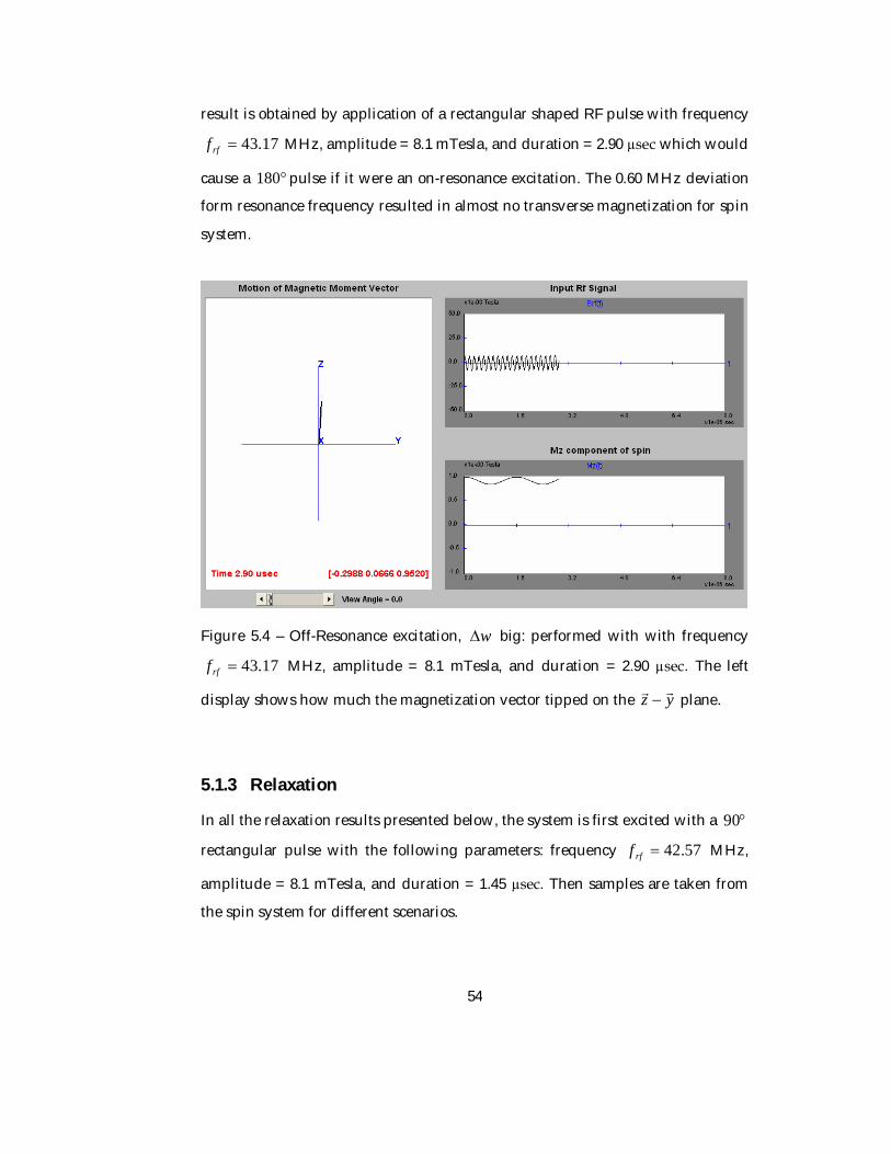
JAVA APPLETS FOR SIMULATION OF MAGNETIC RESONANCE IMAGING
A THESIS SUBMITTED TO THE GRADUATE SCHOOL OF NATURAL AND APPLIED SCIENCES
OF MIDDLE EAST TECHNICAL UNIVERSITY
BY
ÇAĞDAŞ ALTIN
IN PARTIAL FULFILLMENT OF THE REQUIREMENTS FOR
THE DEGREE OF MASTER OF SCIENCE IN
ELECTRICAL AND ELECTRONICS ENGINEERING
DECEMBER 2008
Page 2
Approval of the Thesis:
JAVA APPLETS FOR SIMULATION OF MAGNETIC RESONANCE IMAGING
submitted by ÇAĞDAŞ ALTIN in partial fulfillment of the requirements for the degree of Master of Science in Electrical and Electronics Engineering Department, Middle East Technical University by, Prof. Dr. Canan Özgen Dean, Graduate School of Natural Applied Sciences Prof. Dr. İsmet Erkmen Head of Department, Electrical and Electronics Engineering Prof. Dr. Nevzat G. Gençer Supervisor, Electrical and Electronics Engineering Dept., METU Examining Committee Members Prof. Dr. Murat Eyüboğlu Electrical and Electronics Engineering Dept., METU Prof. Dr. Nevzat G. Gençer Electrical and Electronics Engineering Dept., METU Prof. Dr. Ziya İder Electrical and Electronics Engineering Dept., Bilkent University Assist. Prof. Dr. İlkay Ulusoy Electrical and Electronics Engineering Dept., METU Assist. Prof. Dr. Yeşim Serinağaoğlu Electrical and Electronics Engineering Dept., METU Date : 02/12/2008
Page 3
iii
PLAGIARISM
I hereby declare that all information in this document has been obtained and
presented in accordance with academic rules and ethical conduct. I also declare
that, as required by these rules and conduct, I have fully cited and referenced all
material and results that are not original to this work.
Name, Last name: Çağdaş Altın
Signature :
Page 4
iv
ABSTRACT
JAVA APPLETS FOR SIMULATION OF MAGNETIC RESONANCE IMAGING
Altın, Çağdaş M.S., Department of Electrical and Electronics Engineering
Supervisor: Prof. Dr. Nevzat G. Gençer
December 2008, 88 pages
The aim of this study is to develop an easily accessible and realistic magnetic
resonance imaging (MRI) simulation tool for educational and research purposes.
With this aim, NMR (nuclear magnetic resonance imaging) phenomenon is
simulated based on the physical principles, starting from the motion of a spin
under the influence of external magnetic fields to pulse sequences generating the
image. The inputs of the simulation are a 3D virtual object and a pulse sequence
definition. The simulation software generates slice images using Fourier
reconstruction method. To perform a more realistic simulation, the Bloch
equation, which explains the behavior of a spin under external magnetic fields, is
solved by using numerical methods. This enables to observe the behavior of a
spin system under any magnetic field influence, not only for resonance condition.
The simulation successfully simulates *2T affect by using inhomogeneous static
magnetic field distribution over the entire volume of the object. The software is
implemented in Java language and developed as a Java applet. A support tool is
developed which allows observing NMR phenomenon. The simulation can
produce realistic images, generate many of the artifacts in MRI, like intra-voxel
dephasing, chemical shift, cross-talk (since it simulates the whole process), and
Page 5
v
has the advantage of being web-based compared to the existing stand-alone MRI
simulations.
Keywords: Magnetic resonance imaging, Bloch equation, simulation, Java, applet.
Page 6
vi
ÖZ
MANYETİK REZONANS GÖRÜNTÜLEME BENZETİMİ İÇİN JAVA UYGULAMACIKLARI
Altın, Çağdaş Yüksek Lisans, Elektrik Elektronik Mühendisliği Bölümü
Tez Yöneticisi: Prof. Dr. Nevzat G. Gençer
Aralik 2008, 88 sayfa
Bu çalışmanın amacı, eğitim ve araştırma amaçlı kullanılabilecek, gerçekçi ve
kolay erişilebilir bir manyetik rezonans görüntüleme benzetimi geliştirmektir. Bu
amaçla, NMR (nükleer manyetik rezonans) fenomeni, bir spinin dış manyetik
alanlar altındaki hareketinden başlayıp, darbe dizileri ile görüntü
oluşturulmasına kadar olan bütün süreçleri için, dayandığı fiziksel prensipler
kullanılarak benzetilmiştir. 3 boyutlu bir sanal nesne ve bir darbe dizisi tanımı,
bezetimin girdileridir. Benzetim yazılımı, Fourier geri dönüşüm tekniğini
kullanarak kesit görüntüleri oluşturur. Benzetimin daha gerçekçi sonuçlar
üretmesi için, bir spinin manyetik alan altındaki hareketini açıklayan Bloch
denklemi, sayısal yöntemlerle çözdürülmüştür. Bu sayede spin sisteminin sadece
rezonans durumundaki davranışını değil, her türlü girdi işareti altındaki
davranışını görmek mümkün olmuştur. Benzetimde *2T etkisi, bütün hacimde
homojen olmayan statik manyetik alan dağılımı kullanarak başarılı bir şekilde
benzetilmiştir. Benzetim , Java dilinde yazılmıştır ve bir Java uygulamacığı olarak
geliştirilmiştir. Ayrıca NMR fenomeninin gözlemlenebilmesi için bir destek
yazılımı geliştirilmiştir. Benzetim gerçekçi görüntüler üretebilmekte, bütün
işleyişi benzettiği için MR’daki voksel içi faz dağılması, kimyasal kayma, cross-
Page 7
vii
talk gibi bozulmaları oluşturabilmekte ve hali hazırda tek başına çalışan
benzetimlere göre internet üzerinden çalışma avantajına sahiptir.
Anahtar Kelimeler: Manyetik rezonans görüntüleme, Bloch denklemi, benzetim,
Java, uygulamacık.
Page 8
viii
ACKNOWLEDGEMENT
I would like to express my sincere appreciation to my supervisor Assoc. Prof. Dr.
Nevzat Güneri Gençer for her guidance, advice, criticism, encouragements and
insight throughout the research.
I would like to express my thanks to my friends Suat Gümüşsoy and Cem Şafak
Şahin. Their support and assistance was invaluable.
I would like to thank my dear friends Erol Aran and Yusuf Bediz. It is a great
feeling to know that somebody cares about you and will be by your side in every
situation.
I would like to give my special thanks to Yıldızfer Kemaloğlu for her great
support.
Finally, I would like to thank my family for their understanding, support and
patience; especially to my father and mother.
Page 9
ix
TABLE OF CONTENTS
ABSTRACT .................................................................................................................. iv
ÖZ................................................................................................................................. vi
ACKNOWLEDGEMENT .........................................................................................viii
TABLE OF CONTENTS.............................................................................................. ix
LIST OF FIGURES ....................................................................................................... xi
LIST OF ABBREVIATIONS ...................................................................................... xiii
CHAPTER
1. INTRODUCTION......................................................................................................1
1.1 General............................................................................................................1
1.2 Scope of the thesis..........................................................................................2
1.3 Outline of the dissertation.............................................................................2
2. MRI BASIC PRINCIPLES .........................................................................................4
2.1 Nuclear Magnetic Resonance Phenomenon ................................................4
2.1.1 Nuclear Magnetic Moments ..................................................................4
2.1.2 Bulk Magnetization................................................................................6
2.1.3 Bloch Equation........................................................................................7
2.1.4 Rf Excitation and Resonance .................................................................7
2.1.5 Relaxation ...............................................................................................9
2.2 Image Generation.........................................................................................12
2.2.1 Signal Detection....................................................................................12
2.2.2 Signal Localization ...............................................................................13
3. SIMULATION METHODS .....................................................................................19
Page 10
x
3.1 Overview of Simulator ................................................................................21
3.2 3D Virtual Object Definition .......................................................................22
3.3 Pulse Sequence Controller...........................................................................25
3.3.1 Pulse Sequence Definition ...................................................................25
3.3.2 Simulation Flow ...................................................................................28
3.3.3 Data Collection Parameters .................................................................29
3.4 Bloch Equation Simulator............................................................................30
3.4.1 T2* and T2** Simulation.......................................................................33
3.5 Image Construction .....................................................................................34
4. SIMULATION SOFTWARE ARCHITECTURE AND USER INTERFACE ........36
4.1 Software Architecture..................................................................................37
4.2 Application User Interfaces.........................................................................38
4.2.1 Spin Simulator ......................................................................................38
4.2.2 MRI Simulator ......................................................................................42
5. SIMULATION RESULTS AND DISCUSSION......................................................49
5.1 Results from Spin Simulator .......................................................................49
5.1.1 Resonance .............................................................................................50
5.1.2 Off-Resonance.......................................................................................53
5.1.3 Relaxation .............................................................................................54
5.1.4 Echo Generation ...................................................................................60
5.2 Results from MRI Simulator .......................................................................67
5.2.1 Slice Selection .......................................................................................69
5.2.2 Spin Echo ..............................................................................................73
5.2.3 Gradient Echo.......................................................................................76
5.2.4 Echo Planar ...........................................................................................78
5.2.5 MRI Artifacts ........................................................................................80
6. CONCLUSION ........................................................................................................84
6.1 Summary of the Thesis ................................................................................84
6.2 Discussions and Future Work.....................................................................84
REFERENCES..............................................................................................................88
Page 11
xi
LIST OF FIGURES
Figure 2.1 – The change of zM and xyM during relaxation [2]. .............................11
Figure 2.2 – The affect of gradient fields on the net static magnetic field [2]. ........14
Figure 2.3 – Slice selection selectively excites spins in a region [2]. ........................15
Figure 2.4 – Spin Echo Pulse Sequence [2] ................................................................17
Figure 3.1 – Main building blocks of the simulator..................................................22
Figure 3.2 – 3D Virtual Object composed of three slices. .........................................22
Figure 3.3 – Virtual MRI 3D object class diagram.....................................................23
Figure 3.4 – MRI event processing classes.................................................................26
Figure 3.5 – Event generation from a pulse sequence ..............................................27
Figure 3.6 – Pulse Sequence Controller Flow............................................................28
Figure 3.7 – Bloch Equation Simulator Input/Output Scheme ...............................31
Figure 4.1 – Utility classes to implement a pulse sequence .....................................38
Figure 4.2 – User Interface of Spin Simulator ...........................................................39
Figure 4.3 – User Interface of Spin Simulator while the simulation is running .....42
Figure 4.4 – User Interface of MRI Simulator............................................................43
Figure 4.5 – User Interface of MRI Simulator while simulation is running............47
Figure 5.1 – On-Resonance excitation........................................................................50
Figure 5.2 – On-Resonance excitation with sinc shaped envelope function . ........52
Figure 5.3 – Off-Resonance excitation, w small.....................................................53
Figure 5.4 – Off-Resonance excitation, w big.........................................................54
Figure 5.5 – 2T relaxation for 40 msec with a sampling period of 0.1 msec ...........55
Figure 5.6 – 1T and 2T relaxation...............................................................................56
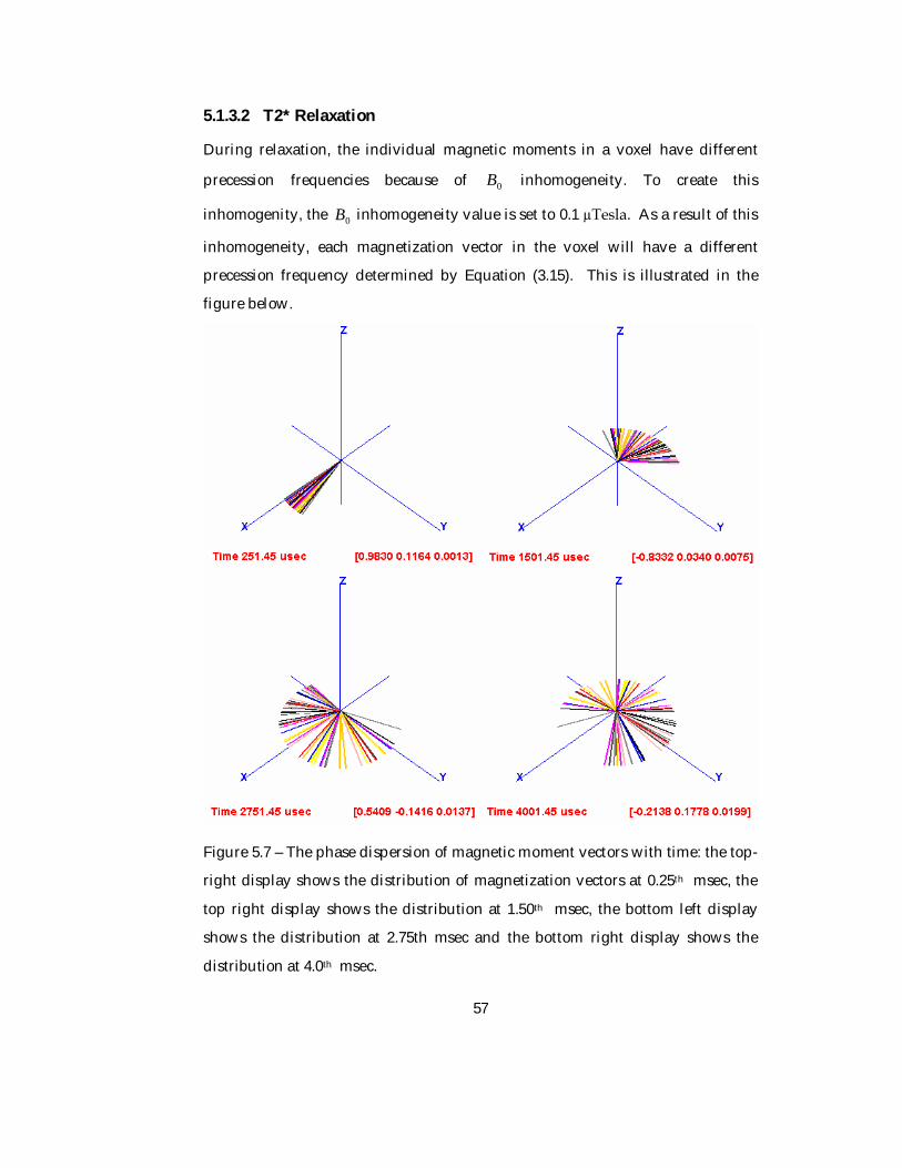
Figure 5.7 – The phase dispersion of magnetic moment vectors with time............57
Figure 5.8 – The decay of )(tM xy vs. t with *2T when B =0.1 µTesla...................58
Page 12
xii
Figure 5.9 – The decay of )(tM xy vs. t with *2T with B =0.2 µTesla.....................59
Figure 5.10 –Phase recovery after 180 pulse...........................................................61
Figure 5.11 – Spin echo simulation ............................................................................61
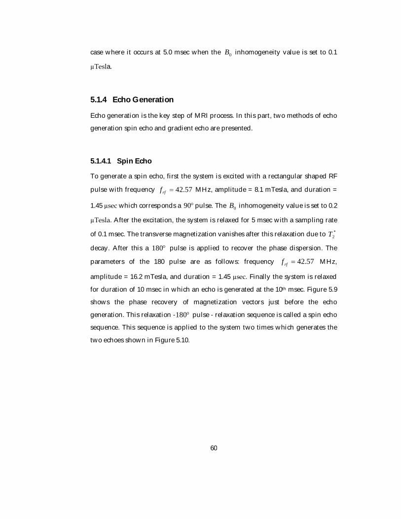
Figure 5.12 – Spin echoes following 2T decay ..........................................................62
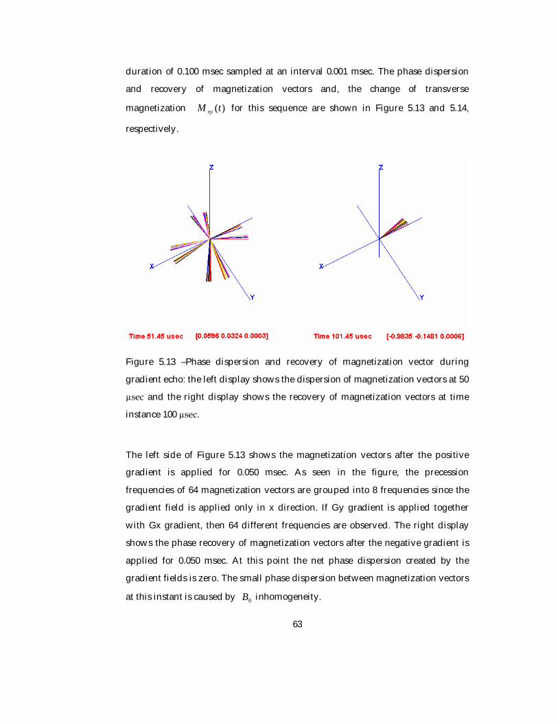
Figure 5.13 –Phase dispersion and recovery of magnetization vector during
gradient echo ...............................................................................................................63
Figure 5.14 – Gradient echo simulation.....................................................................64
Figure 5.15 – Gradient echoes following 2T ..............................................................65
Figure 5.16 – Gradient echoes following *2T .............................................................66
Figure 5.17 –Input objects specification.....................................................................68
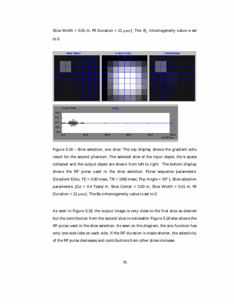
Figure 5.18 – Slice selection, one slice........................................................................70
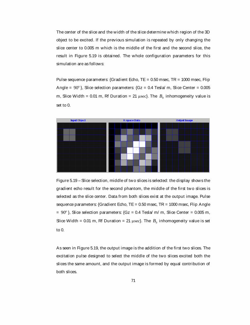
Figure 5.19 – Slice selection, middle of two slices is selected ..................................71
Figure 5.20 – Slice selection with a hard pulse..........................................................72
Figure 5.21 – Spin echo result for the first phantom, proton density weighted.....73
Figure 5.22 – Spin echo result for the first phantom, T2 weighted..........................74
Figure 5.23 – Spin echo result for the second phantom, second slice selected. ......75
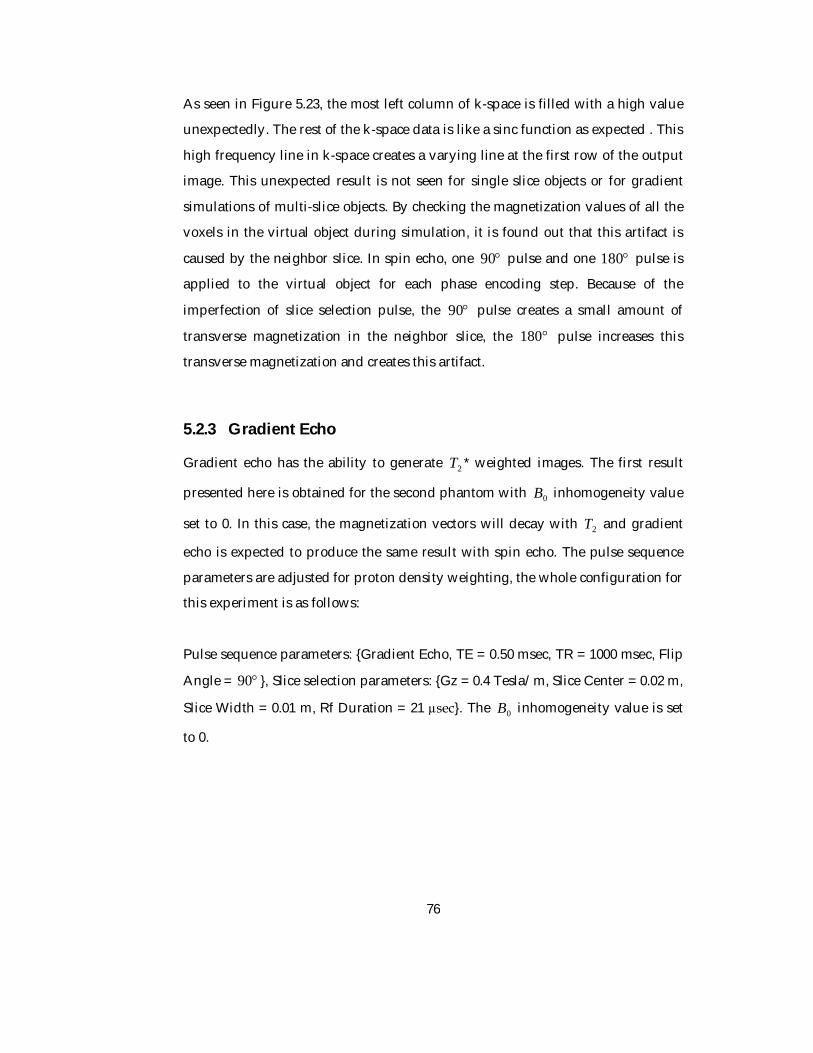
Figure 5.24 – Gradient echo result for the second phantom, third slice selected...77
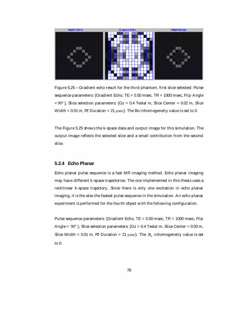
Figure 5.25 – Gradient echo result for the third phantom, first slice selected ........78
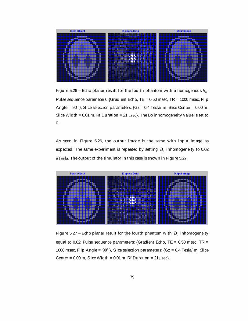
Figure 5.26 – Echo planar result for the fourth phantom with homogenous 0B ...79
Figure 5.27 – Echo planar result for the fourth phantom with 0B inhomogeneity
equal to 0.02 µTesla .....................................................................................................79
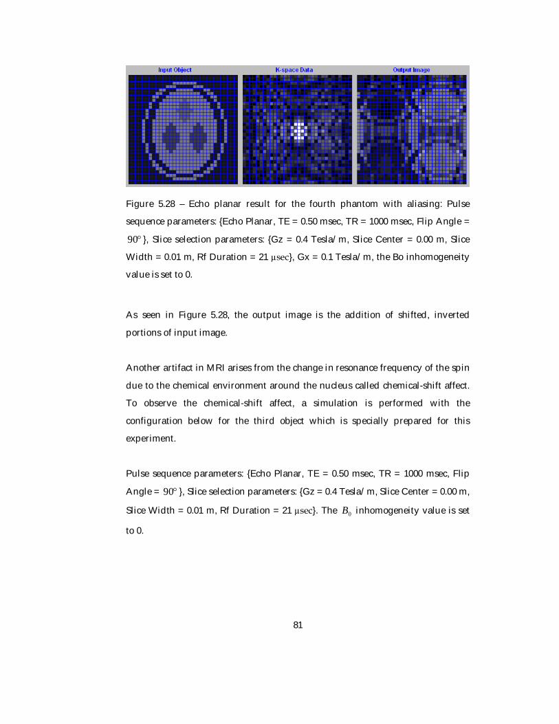
Figure 5.28 – Echo planar result for the fourth phantom with aliasing. .................81
Figure 5.29 – Echo planar result for the third phantom, chemical-shift affect .......82
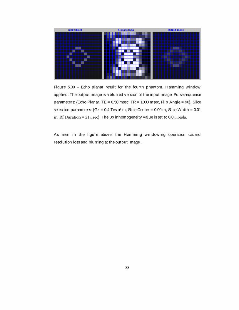
Figure 5.30 – Echo planar result for the fourth phantom, Hamming window
applied .........................................................................................................................83
Page 13
xiii
LIST OF ABBREVIATIONS
2D 2 Dimensional
3D 3 Dimensional
MRI Magnetic Resonance Imaging
NMR Nuclear Magnetic Resonance
PC Personal Computer
RF Radio Frequency
TR Time of Repetition
TE Time of Echo
RAM Random Access Memory
GHz Giga Hertz
MHz Mega Hertz
API Application Programming Interface
Page 14
1
CHAPTER 1
INTRODUCTION
1.1 General
Magnetic Resonance Imaging (MRI) has been a widely used imaging system after
its invention two decades ago, due to its high capability and safety. It has a
number of advantages compared to other non-invasive imaging modalities. These
can be counted as high spatial resolution, high contrast on soft tissues, flexibility
to image more than one parameter of biological tissues, and ability to generate
two-dimensional images at any orientation without changing the position of the
patient. MRI does not use ionizing radiation which can be harmful to the patients.
It operates in radio-frequency (RF) range.
The growth in the usage of MRI scanners clinically, increased the need for
educational and research tools in this area. In MRI, like other non-invasive
imaging systems, physical and chemical properties of the object to be imaged are
measured by applying external inputs. MRI is based on the nuclear magnetic
resonance phenomenon (NMR). Basically, the protons in the body are excited by
external magnetic fields according to the NMR phenomenon and these protons
emit magnetic signals which are processed and transformed into an image. The
whole process, starting from a motion of a proton under external magnetic fields
to pulse sequences that generate the image, is quite complex and has a lot of
parameters that have effects on the information content and quality of the image.
Page 15
2
A software simulation of an MRI system can be very helpful to fully understand
the underlying mechanisms that generate the images in MRI. MRI simulations
generate images of perfectly known objects using the parameters defined by the
user. The simulation can show the effect of these parameters on the image and
can allow the artifacts created by the data collection method to be observed. Thus
MRI simulations can be used for educational purposes in clinical environments.
The simulations can also help students to better understand MRI by visualization
of different blocks. Pulse sequences in MRI are still a research area. MRI
simulations can also be helpful in observing the effectiveness of new pulse
sequences before trying it on a real hardware. There is no universal MRI image
database which can be used by investigators to test post-processing applications.
An MRI simulation can also provide sample data for post-processing applications
which are developed to reduce the artifacts and improve image quality.
1.2 Scope of the thesis
This thesis deals with the problem of developing a realistic and easily accessible
MRI simulator. Besides the goal of being a research tool for engineers, it also aims
to be an education tool for students and clinicians. The simulator in this study
does not aim to simulate all the actors in an MRI system including hardware
components, but it aims to simulate NMR phenomenon in a realistic way and
generate many of the artifacts encountered in practice.
1.3 Outline of the dissertation
In chapter 2, basic principles of MRI are described starting from the NMR
phenomenon to some widely used pulse sequences. This chapter provides the
theoretical background for the simulations.
Page 16
3
The implementation methods and the flowchart of the simulation are presented in
chapter 3. This chapter also includes a literature survey giving a comparison of
this study with previous works about this subject.
The user interfaces and the software architecture of the simulation software are
discussed in chapter 4. This chapter provides a detailed user manual for the
applications developed in this study.
Chapter 5 presents the results of the simulation software for different input
parameters.
Finally, Chapter 6 reports the summary of the study and provides concluding
remarks. Some future work is also suggested in this chapter.
Page 17
4
CHAPTER 2
MRI BASIC PRINCIPLES
This chapter provides a brief theoretical background which is needed to
understand the simulation methods. It is organized in two main sections. The first
chapter explains how the NMR phenomenon works and gives definitions of MRI
terms. The second part explains how the NMR phenomenon is used to generate
images.
2.1 Nuclear Magnetic Resonance Phenomenon
MRI is based on the NMR phenomenon which was found in 1946 by Felix Bloch
and Edward Purcell, both of whom were awarded the Nobel Prize in 1952. After
its discovery, NMR is used by scientists to analyze chemical and physical
properties of molecules. After 1970s, MRI has been discovered by using the NMR
phenomenon with phase and frequency encoding to generate images of the body.
2.1.1 Nuclear Magnetic Moments
All materials consist of nuclei. Nuclei with an odd atomic number have a net
electrical charge due to the unpaired nucleon. Nuclei also rotate around its own
axis possessing an angular momentum J
. This spinning charged object is called a
Page 18
5
spin and creates a magnetic moment
which can be related to the angular
momentum J
with the following relationship.
J
(2.1)
is a nucleus dependent physical constant known as gyromagnetic ratio. A related
constant is 2 and its value is 42.58 MHz/Tesla for a proton ( H1 ). All
clinical use of MRI systems is based on H1 which is one of the main atoms
forming our body. An ensemble of spins of a specific atom constitutes a “spin
system”.
The magnitude of the magnetic moment ( 2mAmpere ) is constant under any
condition but its direction is completely random due to thermal motion unless an
external magnetic field is applied. The following equation explains the physical
motion of a spin under an external magnetic field.
Bdtd
(2.2)
If B
is chosen a static magnetic field defined by zaBB 00 , the spins start to
rotate around 0B
with a frequency which is proportional to the magnitude of 0B
.
0Bwo (2.3)
This precessional frequency 0w is called the Larmor frequency or the resonant
frequency of the spin system. In practice, all the spins of a specific atom may not
have the same Larmor frequency. The group of spins that share the same
resonance frequency is called isochromat. The reasons for having multiple
isochromats for a specific spin are the inhomogeneity of 0B
field, the static
magnetic field distortion due to gyromagnetic ratio difference between tissues,
and the chemical shift effect.
Page 19
6
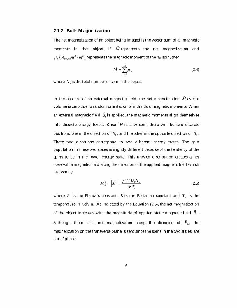
2.1.2 Bulk Magnetization
The net magnetization of an object being imaged is the vector sum of all magnetic
moments in that object. If M
represents the net magnetization and
n ( 32 / mmAmpere ) represents the magnetic moment of the nth spin, then
Ns
nnM
1
(2.4)
where sN is the total number of spin in the object.
In the absence of an external magnetic field, the net magnetization M
over a
volume is zero due to random orientation of individual magnetic moments. When
an external magnetic field 0B
is applied, the magnetic moments align themselves
into discrete energy levels. Since H1 is a ½ spin, there will be two discrete
positions, one in the direction of 0B
, and the other in the opposite direction of 0B
.
These two directions correspond to two different energy states. The spin
population in these two states is slightly different because of the tendency of the
spins to be in the lower energy state. This uneven distribution creates a net
observable magnetic field along the direction of the applied magnetic field which
is given by:
s
sz KT
NBMM4
022
0 (2.5)
where is the Planck’s constant, K is the Boltzman constant and sT is the
temperature in Kelvin. As indicated by the Equation (2.5), the net magnetization
of the object increases with the magnitude of applied static magnetic field 0B
.
Although there is a net magnetization along the direction of 0B
, the
magnetization on the transverse plane is zero since the spins in the two states are
out of phase.
Page 20
7
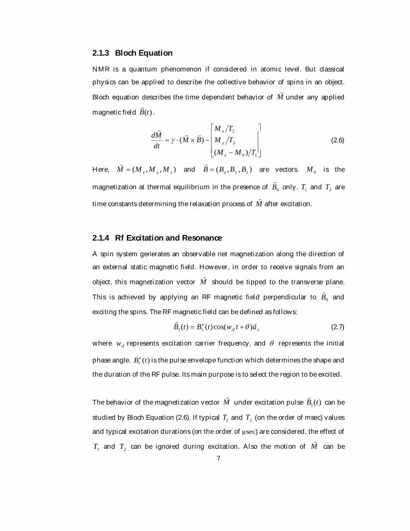
2.1.3 Bloch Equation
NMR is a quantum phenomenon if considered in atomic level. But classical
physics can be applied to describe the collective behavior of spins in an object.
Bloch equation describes the time dependent behavior of M
under any applied
magnetic field )(tB
.
10
2
2
)()(
TMMTMTM
BMdtMd
z
y
x
(2.6)
Here, ),,( zyx MMMM
and ),,( zyx BBBB
are vectors. 0M is the
magnetization at thermal equilibrium in the presence of 0B
only. 1T and 2T are
time constants determining the relaxation process of M
after excitation.
2.1.4 Rf Excitation and Resonance
A spin system generates an observable net magnetization along the direction of
an external static magnetic field. However, in order to receive signals from an
object, this magnetization vector M
should be tipped to the transverse plane.
This is achieved by applying an RF magnetic field perpendicular to 0B
and
exciting the spins. The RF magnetic field can be defined as follows:
xrfe atwtBtB
)cos()()( 11 (2.7)
where rfw represents excitation carrier frequency, and represents the initial
phase angle. )(1 tBe is the pulse envelope function which determines the shape and
the duration of the RF pulse. Its main purpose is to select the region to be excited.
The behavior of the magnetization vector M
under excitation pulse )(1 tB
can be
studied by Bloch Equation (2.6). If typical 1T and 2T (on the order of msec) values
and typical excitation durations (on the order of µsec) are considered, the effect of
1T and 2T can be ignored during excitation. Also the motion of M
can be
Page 21
8
observed more simply in a rotating frame. So if we consider a reference frame
rotating around the z axis with angular velocity w , Equation (2.6) takes the
following form for M
.
effrotrot BM
dtMd
(2.8)
where
wBB roteff
(2.9)
Here, rotM
and rotB
are the magnetization vector and the net external magnetic
field vector at rotating frame respectively. If the rotating frame is rotating at the
Larmor frequency 0w , then zaBw 0 . If only 0B
is applied, then rotB
becomes
zrot aBB 0 and the effective magnetic field effB
becomes
000
z
zeffaB
aBB
. If effB
is zero, then rotM
seems stationary in the rotating
frame according to Equation (2.8).
If )(1 tB
is applied with a carrier frequency equal to 0w , effB
becomes
)()( 10
10 tBaBtBaBB ezzeff
. This input causes a precession motion about
the 1B
field and the magnetization vector tilts away from the z axis. The direction
of )(1 tB
should be perpendicular to static magnetic field 0B
. If the direction of
)(1 tB
is along x , the motion of M
in the rotating frame is governed by:
t
ezy
te
zy
x
dttBMtM
dttBMtM
tM
01
0
01
0
)(cos)(
)(sin)(
0)(
(2.10)
Page 22
9
If )(1 tBe
is a rectangular envelope function, the rotational frequency of this
precession will be 11 Bw
. The amount of the tip angle is determined by the
area under the envelope function:
pT e dttB
0 1 )( (2.11)
The carrier frequency rfw being equal to Larmor frequency 0w is called as the
resonance condition. From a quantum perspective, the resonance excitation
causes the spins at the lower energy state to switch to the higher energy state.
This is achieved by exciting the spins with an amount of energy exactly equal to
cause a transition from one state to another.
If the carrier frequency rfw is different from the resonance frequency 0w , then
the effective field for the spin in rfw rotating frame becomes:
)()()( 1010 tBawtBaw
BB zzrf
eff
(2.12)
In this case, the effective field has a vertical and horizontal component. For a
rectangular shaped )(1 tB
, the effective field effB
points along the resultant vector
of 0w and the magnitude of )(1 tB
. The magnetization vector again rotates
around this effective field. If 1Bwo , then the effective field becomes close to
0B
and the magnetization vector does not tilt away from the z axis significantly.
This is called off-resonance excitation.
2.1.5 Relaxation
The RF magnetic field )(1 tB
is the external force that perturbs the magnetized
spin system from its thermal equilibrium value by flipping the magnetization
vector into the transverse plane. When this external energy is turned off, the
magnetization vector returns to its initial position by making a precession motion
about 0B
. This process is called relaxation and it is characterized by the recovery
Page 23
10
of longitudinal magnetization zM and the decay of transverse magnetization
xyM .
When the RF field is turned off, the effective field effB
seen by the magnetization
vector in the Larmor rotating frame becomes 000
z
zeffaBaBB
. Then the
Bloch equation reduces to:
2
1
0
TM
dM
TMMdM
xyxy
zzz
(2.13)
where 1T is called the spin-lattice relaxation time and 2T is spin-spin relaxation
time. The following are the solution of the above equation.
tiwTt
xyxy eeMtM 02)0()(
(2.14)
11 )0()1()( 0 Tt
zT
t
zz eMeMtM
(2.15)
where )0( xyM and )0( zM are magnetizations on the transverse plane and
along the z axis just after the RF pulse. Equation (2.14) indicates that the
transverse magnetization xyM makes a precession motion on the transverse plane
around z axis and its magnitude decays exponentially at a rate determined by
2T . As stated in Equation (2.15), the longitudinal magnetization zM recovers its
equilibrium value 0zM exponentially at a rate determined by 1T . The decay of
xyM and the recovery of zM during relaxation are shown on the Figure (2.1)
below.
Page 24
11
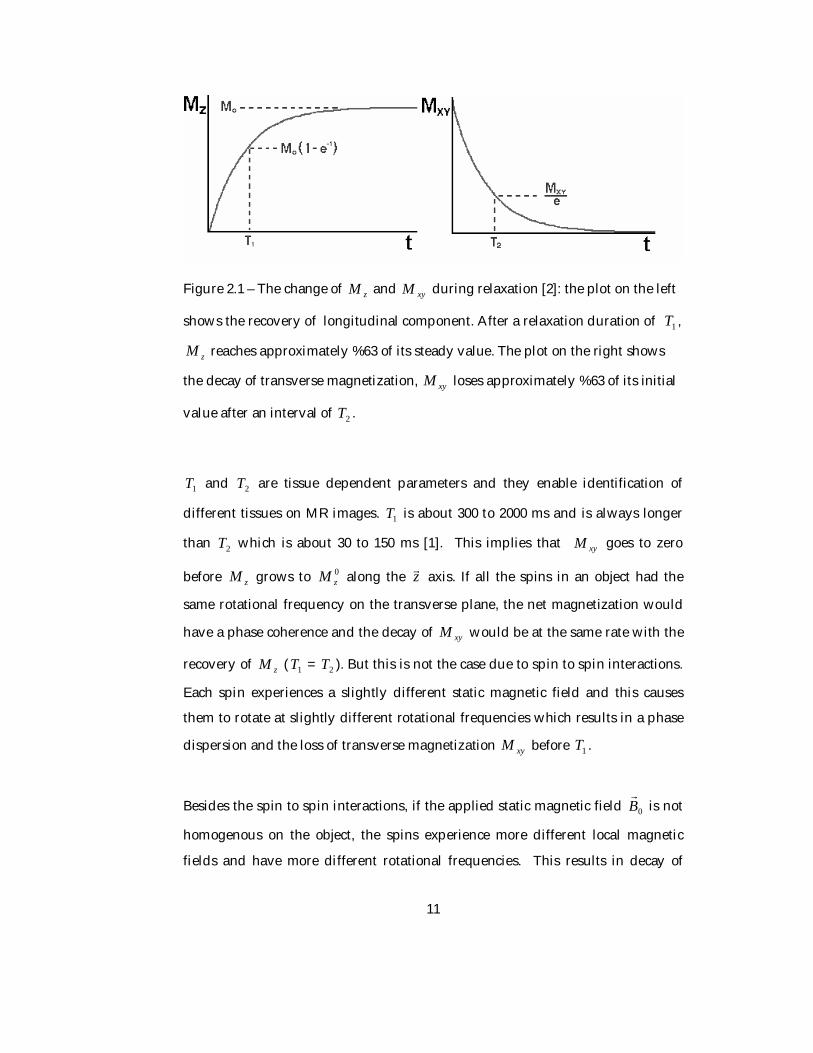
Figure 2.1 – The change of zM and xyM during relaxation [2]: the plot on the left
shows the recovery of longitudinal component. After a relaxation duration of 1T ,
zM reaches approximately %63 of its steady value. The plot on the right shows
the decay of transverse magnetization, xyM loses approximately %63 of its initial
value after an interval of 2T .
1T and 2T are tissue dependent parameters and they enable identification of
different tissues on MR images. 1T is about 300 to 2000 ms and is always longer
than 2T which is about 30 to 150 ms [1]. This implies that xyM goes to zero
before zM grows to 0zM along the z axis. If all the spins in an object had the
same rotational frequency on the transverse plane, the net magnetization would
have a phase coherence and the decay of xyM would be at the same rate with the
recovery of zM ( 1T = 2T ). But this is not the case due to spin to spin interactions.
Each spin experiences a slightly different static magnetic field and this causes
them to rotate at slightly different rotational frequencies which results in a phase
dispersion and the loss of transverse magnetization xyM before 1T .
Besides the spin to spin interactions, if the applied static magnetic field 0B
is not
homogenous on the object, the spins experience more different local magnetic
fields and have more different rotational frequencies. This results in decay of
Page 25
12
xyM earlier than 2T . This decay rate is called *2T . In practice, the net
magnetization on the transverse plane xyM never decays with 2T but with *2T .
The inhomogeneity of 0B
is not the only reason behind *2T . The chemical shift
effect and the magnetic susceptibility variations on the boundaries of the tissues
are the other reasons of *2T decay [1, 3].
2.2 Image Generation
If an object is placed in an external magnetic field 0B
and excited with an RF
magnetic field )(1 tB
, the magnetization vector M
flips into transverse plane.
After the alternating magnetic field )(1 tB
is turned off, the magnetization vector
M
returns to its equilibrium position by making a precessional motion around
0B
. This is briefly the NMR phenomenon. Now the question is how to generate
an image using NMR.
This section explains the process that produces the MR image starting from the
signal detection to pulse sequences.
2.2.1 Signal Detection
In MRI, the net magnetization vector M
starts rotating at an RF frequency on the
transverse plane after the RF magnetic field )(1 tB
is turned off. This
magnetization can be detected by placing a coil along the object. By Faraday’s law
of electromagnetic induction, this rotating magnetization will induce a voltage at
the receiver coil that is equal to the rate at which the flux through the coil is
changing. The voltage in the coil can be expressed as:
drtrMrBtt
ttVobject r
),()()()( (2.16)
Page 26
13
where )(t is the flux through the coil and )(rBr
and )(rM r
are the magnetic
flux density and magnetization vector at the spatial position r respectively.
Assuming that the receiver has a homogenous reception sensitivity over the
region of interest and considering that )(tM z is a slowly varying function, the
received signal equation turns into the integration of transverse magnetization
xyM over the entire volume.
object xyxy drtrMdxdydztzyxMtS ),(),,,()( (2.17)
where )(tS is the received signal. Considering the relaxation equation of
transverse magnetization (2.14), this equation can be written as:
object
triwrTt
xy dreerMtS )()(2)0,()( (2.18)
The signal received at the coil is a high frequency signal which can cause
problems for electronic circuitries [1]. In practice, this signal is moved to baseband
by signal demodulation method. This method multiplies the input signal with a
reference signal and removes the high frequency component by low-pass
filtering. In MRI, this reference signal is a sinusoid at the Larmor frequency. This
demodulation operation converts the signal equation into:
object
trwirTt
xy dreerMtS )()(2)0,()( (2.19)
where 0)()( wrwrw .
2.2.2 Signal Localization
Equation (2.17) tells us that the received signal is the sum of all local
magnetization vectors in the object. If all these magnetization vectors had the
same rotating frequency )(rw , the received signal )(tS would have only
frequency component and would not give any spatial information. To be able to
obtain spatial information, gradient fields are used which are defined as:
zzyxG azGyGxGzyxB )(),,( (2.20)
Page 27
14
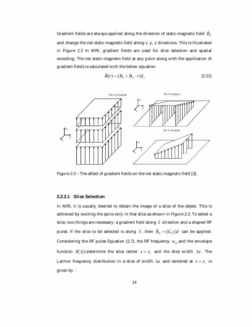
Gradient fields are always applied along the direction of static magnetic field 0B
and change the net static magnetic field along x, y, z directions. This is illustrated
in Figure 2.2 In MRI, gradient fields are used for slice selection and spatial
encoding. The net static magnetic field at any point along with the application of
gradient fields is calculated with the below equation.
zG arBBrB )()( 0 (2.21)
Figure 2.2 – The affect of gradient fields on the net static magnetic field [2].
2.2.2.1 Slice Selection
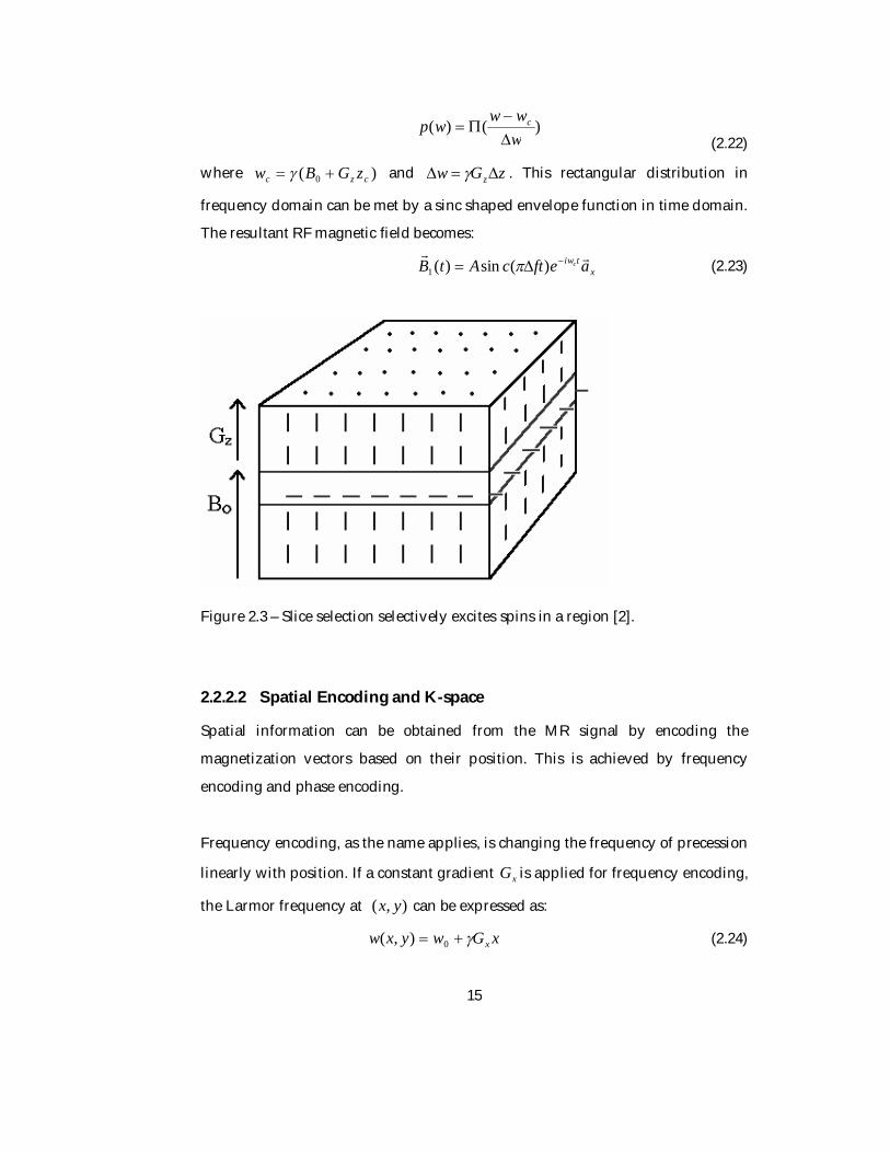
In MRI, it is usually desired to obtain the image of a slice of the object. This is
achieved by exciting the spins only in that slice as shown in Figure 2.3. To select a
slice, two things are necessary: a gradient field along z direction and a shaped RF
pulse. If the slice to be selected is along z , then zzGB zG
)( can be applied.
Considering the RF pulse Equation (2.7), the RF frequency rfw and the envelope
function )(1 tB e determine the slice center czz and the slice width z . The
Larmor frequency distribution in a slice of width z and centered at czz is
given by :
Page 28
15
)()(wwwwp c
(2.22)
where )( 0 czc zGBw and zGw z . This rectangular distribution in
frequency domain can be met by a sinc shaped envelope function in time domain.
The resultant RF magnetic field becomes:
xtiw aeftcAtB c
)(sin)(1 (2.23)
Figure 2.3 – Slice selection selectively excites spins in a region [2].
2.2.2.2 Spatial Encoding and K-space
Spatial information can be obtained from the MR signal by encoding the
magnetization vectors based on their position. This is achieved by frequency
encoding and phase encoding.
Frequency encoding, as the name applies, is changing the frequency of precession
linearly with position. If a constant gradient xG is applied for frequency encoding,
the Larmor frequency at ),( yx can be expressed as:
xGwyxw x 0),( (2.24)
Page 29
16
When frequency encoding is applied, contributions of magnetization vectors at
different locations along x will have different precessional frequencies.
Phase encoding is the same as frequency encoding except that it is applied for a
short interval peT and then it is turned off. As a result of this, signals from
different locations will have different phase angles. If a constant gradient yG is
applied for phase encoding, the Larmor frequency will be yGwyxw y 0),(
during the interval peTt 0 . The total phase accumulated at the end of this
interval will be:
peype yTGT )( (2.25)
If both frequency encoding and phase encoding are applied during an MRI signal
acquisition, and if 2T relaxation is ignored, the baseband signal equation
becomes:
dxdyerMdreerMtS peyx yTGxtGixyobject
rtriwrTt
xy)()()()( )0,()0,()( 2 (2.26)
If we denote tGk xx and peyy TGk , then the signal equation turns into:
dxdyeyxMktkStS ykxki
xyyxyx )()0,,()),(()( (2.27)
As seen in Equation (2.27), the signal equation is the Fourier transform of
magnetization at time t . After phase encoding interval, each voxel along the y
direction has a distinct phase although they have the same precession frequency.
The frequency encoding causes every location along x direction to have a distinct
precession frequency during readout. This distinct pair of a phase and a
frequency of the magnetization precession converts the received signal into the
Fourier transform of the magnetization.
2.2.2.3 Pulse Sequences
The signal measured in Equation (2.27) contains samples from one row of spatial
frequency space ),( yx kk , also called as the K-space in MRI literature. The
Page 30
17
relationship between frequency domain and time domain is same for K-space and
spatial domain. If all rows of K-space are filled by taking measurements of )(tS
with different values of yG , the Fourier transform of the magnetization function
),( yxM is obtained. Then one can apply inverse Fourier transform operation to
obtain the magnetization function ),( yxM :
),(),( 1yx kkSFyxM (2.28)
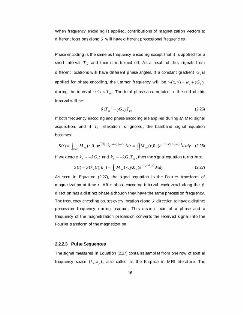
To fill another row in K-space, the system should be excited again and a readout
must be performed witch switches to another row in K-space by use of gradients.
The sequence of these excitation and readout events are called as a pulse
sequence. An example of a pulse sequence is shown in Figure 2.4. The time
between two consecutive excitations is called time of repetition (TR).
Figure 2.4 – Spin Echo Pulse Sequence [2]: the echo time TE is the duration where
the readout signal reaches its peak value, the pulse sequence above is applied
number of phase encoding steps times where each step performed in TR duration.
Page 31
18
It is more convenient to express ),( yxM in (2.28) as the imaging function rather
than the magnetization function since it is a function of proton density p and
relaxation constants 1T and 2T . By changing the parameters of the pulse
sequence, it is possible to weight the received signal ),( yxM with one of these
tissue properties.
Page 32
19
CHAPTER 3
SIMULATION METHODS
Simulations should be close to reality in order to be useful. The simulation
system proposed in his thesis, aims to create a flexible and expandable simulation
framework which takes into account most of the physical processes in MRI.
Many MRI simulations have been developed so far by different research groups
[3-7]. These simulators have different approaches in modeling the reality,
methods of implementation and software design. The previous simulators can
mainly be divided into two groups.
Some simulators generate new images from known images by using the image
intensity functions of pulse sequences. The image intensity functions depend on
spin parameters; proton density, 1T and 2T and pulse sequence parameters; flip
angle, time of echo ET and time of repetition RT [7]. These simulations are helpful
in observing the image contrast variation with pulse sequence parameters.
However, this approach does not simulate the whole process of MRI and thus is
not able to simulate all the artifacts like chemical-shift, intra-voxel dephasing,
imperfection of slice selection, aliasing, non-linear gradients, 0B inhomogeneity
and susceptibility artifacts. Some of these simulators generate k-space data by
taking the Fourier transform of the input parameter image and modify the k-
Page 33
20
space data to generate the artifacts encountered in MRI. Then by taking the
inverse Fourier transform, output images are obtained.
Another group of simulators is based on the solution of Bloch equation for virtual
objects which are composed of small volume elements called voxels, each
representing a magnetization for a specific spin [3, 4, 6]. Depending on the pulse
sequence parameters selected, the magnetization for each voxel is calculated
according to the Bloch equation and the summation of these magnetizations yield
the MR signal. This approach is the closest model to reality since it is a discrete
representation of the real process. In this thesis, this model is followed. This
model is only limited by the Bloch equation which ignores some physical events
like diffusion. This approach suffers from high computation times due to the need
of large number of magnetization vectors to correctly represent the virtual object.
Some simulators make use of the computation power of parallel processing to
decrease the high computation times [4,6]. The spin model and the Bloch equation
are appropriate for such a distributed node implementation.
The Bloch equation based simulators take the virtual object definition and pulse
sequence parameters from the user and generate the MR signal by a Bloch
equation solver. These simulators differ in the solution of Bloch equation and
generation of echoes. Some simulators calculate the magnetization values using
rotational and scaling matrix operations corresponding to excitation, relaxation
and gradient field affects. Analytical solution of Bloch equation is used for
calculation of flip angle values which is an acceptable approach if the step size is
chosen small enough [3,6]. In [3], a hybrid approach is used where numerical
methods are used when the analytic solution does not exist for the Bloch
equations and analytic solution is preferred other times.
A simulation should be able to generate the artifacts created by the actors in a
physical process to be close to reality. In MRI, these artifacts can be counted as:
chemical-shit effect, 0B inhomogeneity, RF magnetic field inhomogeneity, non-
Page 34
21
linear gradients, aliasing, imperfection of slice selection, intra-voxel dephasing,
and Gibbs phenomenon. To simulate the artifacts, the sources that create these
artifacts must be modeled in a realistic way.
To generate echoes, Benoit [4] uses a tricky method which reduces the number of
magnetization vectors per voxel but is based on the assumption of a Lorentzian
distribution for static magnetic field inhomogeneity. This approach is very
interesting since it allows generation of echoes using only one magnetization
vector per voxel. Yoder [3] includes magnetic susceptibility variations besides
static magnetic field inhomogenity to simulate local magnetic field variations.
This is a more realistic approach to simulate intra-voxel dephasing but requires
processing of the virtual objects to calculate susceptibility changes before the
simulation. In this study, intra-voxel dephasing is realized by changing local
magnetic fields using 0B inhomogeneity.
There is only one web based MRI simulator in the literature [8]. It is also a Java
applet which is accessible through internet. This simulator is very helpful for
teaching MRI contrast behavior but it is in the group of k-space based simulators
which lacks generality. The other Bloch equation based simulators [3,4] perform
realistic simulations but are either stand-alone PC application for specific
platforms or require special hardware to run simulations. The simulation
software developed in this study is the first Bloch equation based, web accessible
MRI simulator in the literature.
3.1 Overview of Simulator
The simulation software is composed of four main building blocks shown in
Figure 2.2. Among these blocks the 3D virtual object definition and Pulse
sequence definition blocks are the ones that the user provides as input to the
simulation. The Bloch equation simulation block is the kernel of the simulation
Page 35
22
and generate the MRI signal by using the input blocks. The image construction
block processes the received signal and generates the image function.
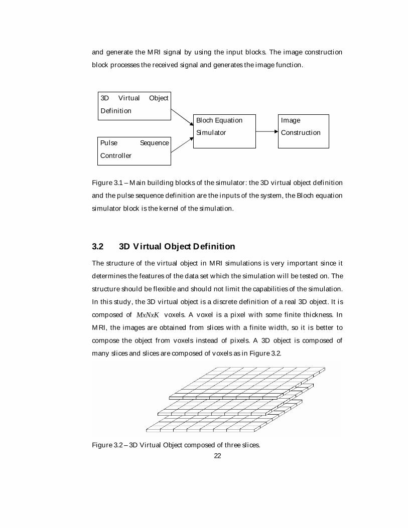
Figure 3.1 – Main building blocks of the simulator: the 3D virtual object definition
and the pulse sequence definition are the inputs of the system, the Bloch equation
simulator block is the kernel of the simulation.
3.2 3D Virtual Object Definition
The structure of the virtual object in MRI simulations is very important since it
determines the features of the data set which the simulation will be tested on. The
structure should be flexible and should not limit the capabilities of the simulation.
In this study, the 3D virtual object is a discrete definition of a real 3D object. It is
composed of MxNxK voxels. A voxel is a pixel with some finite thickness. In
MRI, the images are obtained from slices with a finite width, so it is better to
compose the object from voxels instead of pixels. A 3D object is composed of
many slices and slices are composed of voxels as in Figure 3.2.
Figure 3.2 – 3D Virtual Object composed of three slices.
3D Virtual Object
Definition
Pulse Sequence
Controller
Bloch Equation
Simulator
Image
Construction
Page 36
23
Voxels are defined cubical so one dimension is enough. A voxel has a 3D position
information defined in Cartesian coordinates (x, y, z) and contains magnetization
information for a spin. The voxel holds a proton density value ip and the spin
information which is defined with the following properties: gyromagnetic ratio
, and the relaxation constants 1T and 2T . The spin information changes from
tissue to tissue. In a voxel, the magnetization is represented by one or a group of
magnetization vectors. Each magnetization vector has 3D position information
and holds a 3D vector for magnetization value. The positions of the magnetization
vectors are determined by distributing them evenly in the voxel. A clearer picture
of the structure of the virtual object is given with the following UML class
diagram in Figure 3.3.
Figure 3.3 – Virtual MRI 3D object class diagram: as shown on the figure, the 3D
virtual object class holds multiple voxel objects and the voxel class holds multiple
magnetization vector objects, each voxel object has one spin and voxel and
magnetization vector objects have position information.
Page 37
24
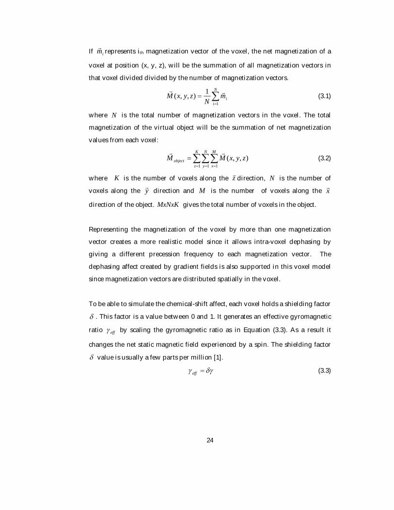
If im represents ith magnetization vector of the voxel, the net magnetization of a
voxel at position (x, y, z), will be the summation of all magnetization vectors in
that voxel divided divided by the number of magnetization vectors.
N
iim
NzyxM
1
1),,( (3.1)
where N is the total number of magnetization vectors in the voxel. The total
magnetization of the virtual object will be the summation of net magnetization
values from each voxel:
K
z
N
y
M
xobject zyxMM
1 1 1),,(
(3.2)
where K is the number of voxels along the z direction, N is the number of
voxels along the y direction and M is the number of voxels along the x
direction of the object. MxNxK gives the total number of voxels in the object.
Representing the magnetization of the voxel by more than one magnetization
vector creates a more realistic model since it allows intra-voxel dephasing by
giving a different precession frequency to each magnetization vector. The
dephasing affect created by gradient fields is also supported in this voxel model
since magnetization vectors are distributed spatially in the voxel.
To be able to simulate the chemical-shift affect, each voxel holds a shielding factor
. This factor is a value between 0 and 1. It generates an effective gyromagnetic
ratio eff by scaling the gyromagnetic ratio as in Equation (3.3). As a result it
changes the net static magnetic field experienced by a spin. The shielding factor
value is usually a few parts per million [1].
eff (3.3)
Page 38
25
3.3 Pulse Sequence Controller
This block controls the timing and order of the events and sets the magnetic input
signals for each event based on the pulse sequence type and parameters selected.
It also calculates the data acquisition parameters according to the input object and
pulse sequence parameters. It takes the pulse definition as input, splits the total
sequence into MRI events which will be explained below, and processes each
event in the sequence consecutively.
3.3.1 Pulse Sequence Definition
The pulse sequence parameters provided by the user are TE (time of echo), TR
(time of repetition) and flip angle value. Three types of pulse sequences are
implemented in the simulation. These are spin echo, gradient echo, and echo
planar pulse sequences.
There are two types of events for a magnetized spin system from the point of
applied magnetic fields. These are excitation and relaxation events. A
combination of these events creates a pulse sequence. Excitation event is the one
which the system is excited with an RF magnetic field. Relaxation event
corresponds to the relaxation of the system with the RF magnetic field off.
Gradient fields may be on or off in both events. A special case of relaxation event
is the readout case where samples are collected from the system and stored in a
buffer for processing. Excitation event is defined mostly by the RF magnetic field
parameters including frequency, amplitude, duration, envelope function type and
bandwidth. Gradient field values are also parameters for excitation event.
Relaxation event is defined with the gradient field parameters and duration. If
readout is going to be performed during relaxation, sampling time is also
provided. The simulation software has 3 classes that handle the processing of
these events shown on Figure 3.4. A combination of these event processing
functions executed consecutively for a virtual object generate a pulse sequence.
Page 39
26
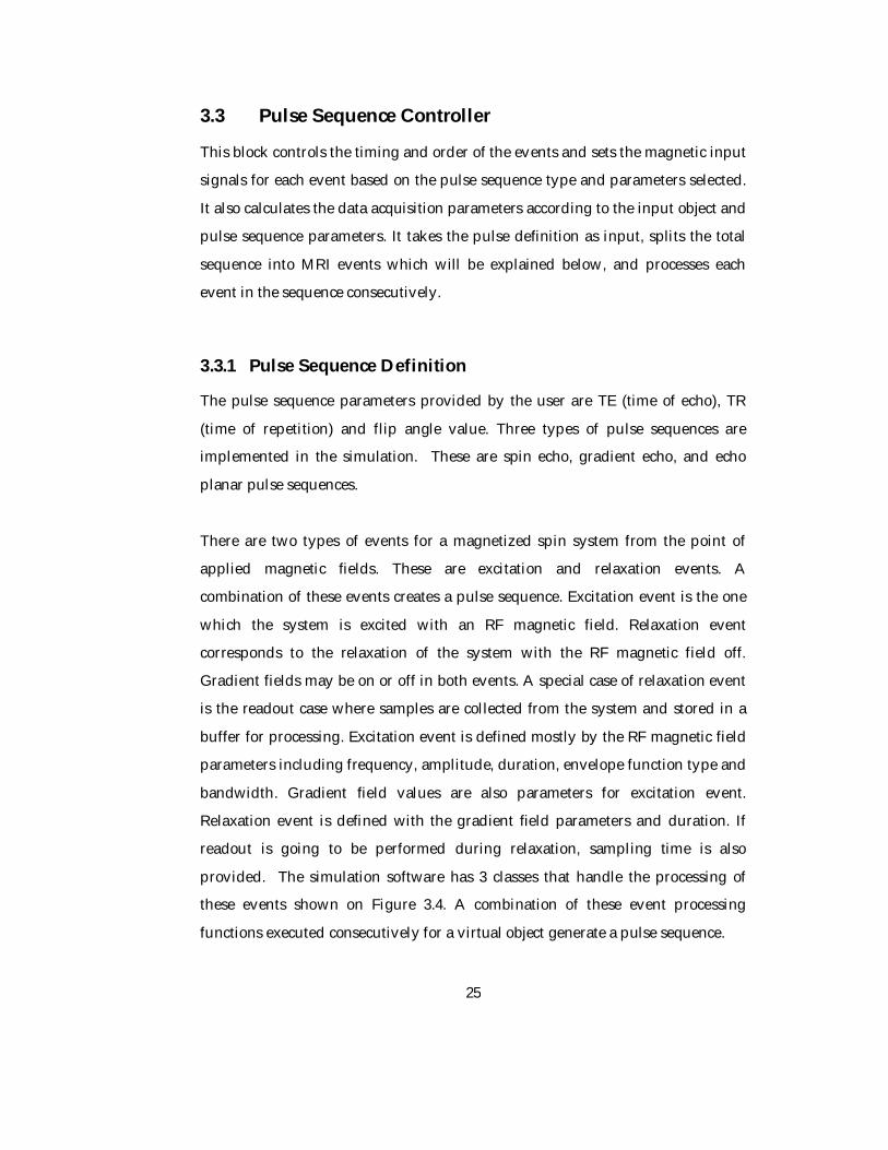
Figure 3.4 – MRI event processing classes: the base class cMriEvent class is an
interface for relaxation and excitation event classes, the polymorphic structure for
MRI event classes enables the event objects to be put in a list and executed
consecutively, the cReadoutEvent class is derived from cRelaxationEvent class
since it is a special form of relaxation event.
To perform a simulation, the pulse sequence controller creates events according to
pulse sequence type selected and its parameters. Figure 3.5 shows how a pulse
sequence is divided into events. Excitation events are only defined for time
regions where RF magnetic field is enabled. The remaining time regions are
divided into relaxation events, each corresponding to a different combination of
gradient fields. If k-space is to be filled during relaxation, it becomes a readout
event.
Page 40
27
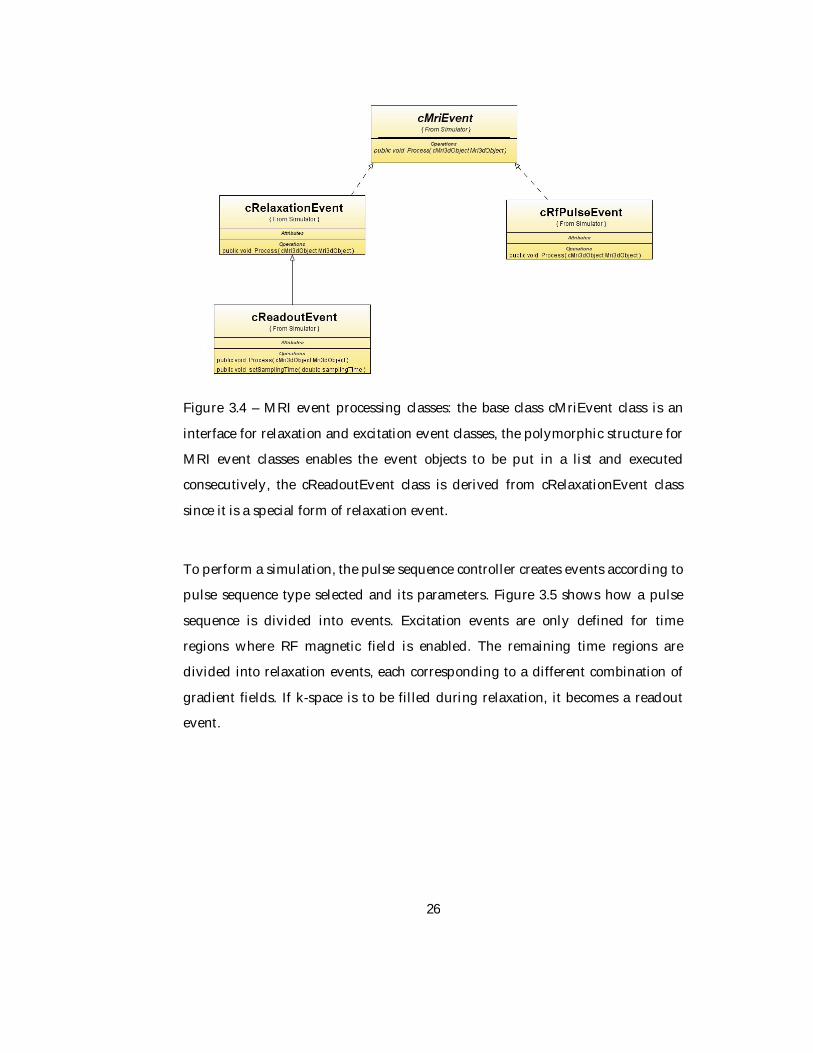
Figure 3.5 – Event generation from a pulse sequence: the spin echo pulse sequence
above is represented with 2 excitation events, 5 relaxation events and 1 readout
event, each relaxation event corresponds to a different combination of gradient
fields.
Three types of magnetic inputs exist in MRI. These are static magnetic field 0B
,
RF magnetic field 1B
and the gradient field GB
. The RF magnetic field is defined
by its carrier frequency, amplitude, duration, and envelope function shape. The
simulation program allows two types of envelope functions to be selected:
rectangular and sinc. If the envelope function is sinc shaped, the bandwidth value
f in Equation (2.23) is calculated. The gradients fields are defined by their
amplitude ),,( zyx GGGG and their duration.
Page 41
28
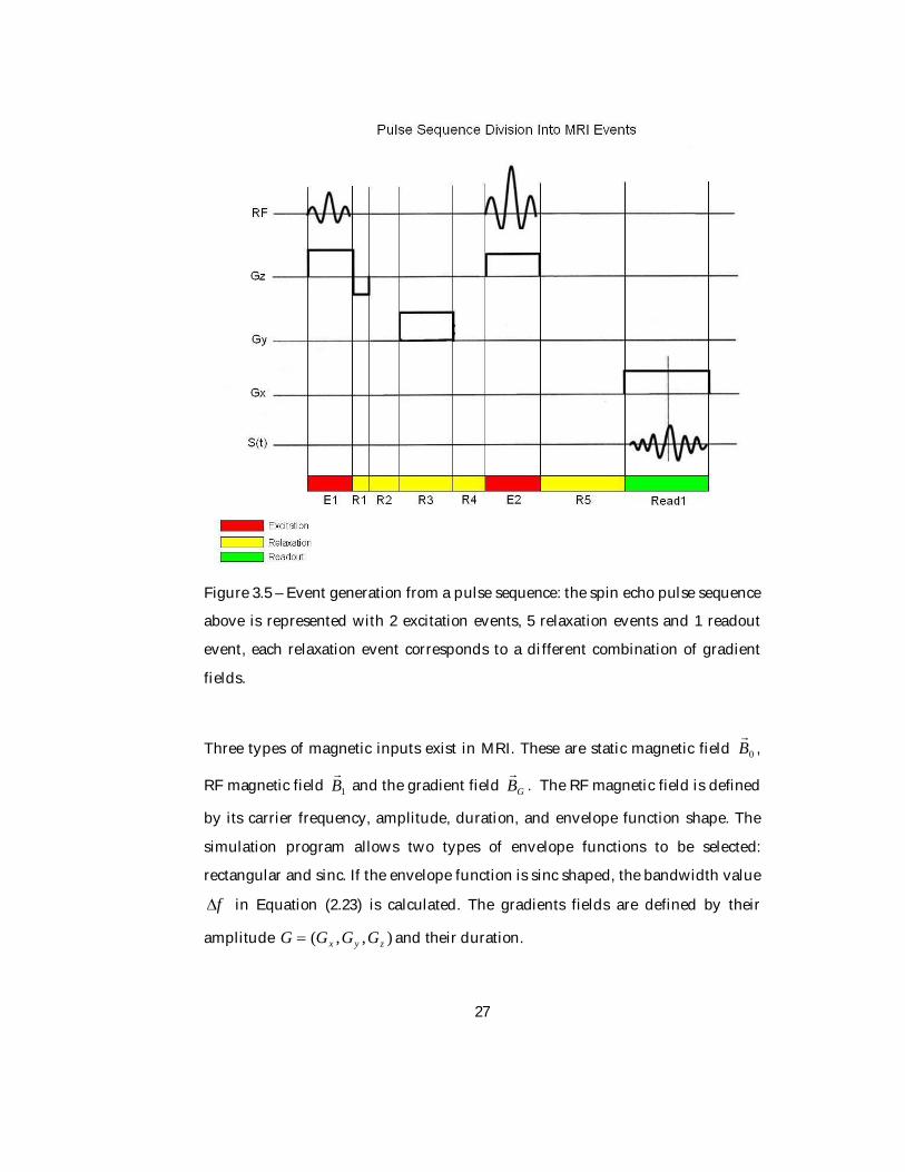
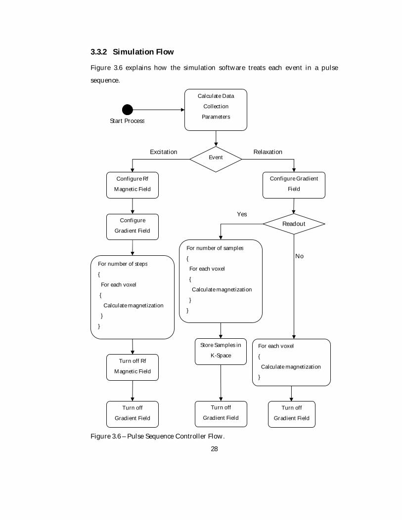
3.3.2 Simulation Flow
Figure 3.6 explains how the simulation software treats each event in a pulse
sequence.
Figure 3.6 – Pulse Sequence Controller Flow.
Calculate Data
Collection
Parameters
For number of steps
{
For each voxel
{
Calculate magnetization
}
}
For each voxel
{
Calculate magnetization
}
Readout
Turn off
Gradient Field
Configure Gradient
Field
Turn off
Gradient Field
Turn off
Gradient Field
No
Configure Rf
Magnetic Field
Configure
Gradient Field
Event Excitation Relaxation
For number of samples
{
For each voxel
{
Calculate magnetization
}
}
Turn off Rf
Magnetic Field
Yes
Store Samples in
K-Space
Start Process
Page 42
29
The simulation software executes the events in a pulse sequence consecutively.
Before a pulse sequence process is started, firstly data collection parameters are
calculated. After this the first event is taken from the list. Each event configures
the magnetic inputs before processing and turns them off after processing. The RF
magnetic field 1B
and the gradient field GB
are configured in an excitation event.
Relaxation and readout events only configure gradient fields. After the magnetic
inputs are configured, the new magnetization values for each voxel in the object
are calculated by the Bloch equation simulator block.
After all the events are processed in a pulse sequence, the k-space buffer is
processed to obtain the image function.
3.3.3 Data Collection Parameters
Data collection parameters are calculated to meet the Nyquist theorem for K-
space sampling. Nyquist theorem states that a signal should be sampled at a rate
at least twice the bandwidth of the signal in order to reconstruct the signals from
its samples again. The signal K-space sampling intervals xk and yk are
determined as follows:
yy
xx
WkWk
11
(3.4)
where xW and yW are the width and the length of the virtual object. The
sampling time is found using the equation tGk xx . Frequency encoding
gradient xG is defined by the user. Then sampling time t becomes:
xx Gkt (3.5)
After this, the step size of phase encoding gradient value is determined by using
the equation below:
peyy TkG (3.6)
Page 43
30
where peT is the phase encoding gradient duration. This parameter is chosen to be
half of the data acquisition time. Data acquisition time is equal to the number of
voxels along the frequency encoding direction times the sampling time t .
3.4 Bloch Equation Simulator
The Bloch equation simulation is the heart of an MRI simulation program since it
calculates the net magnetization from the virtual object and generates the K-space
data. This block performs the task of “calculation magnetization values” in the
pulse sequence flow in Figure 3.6. The input-output scheme of Bloch equation
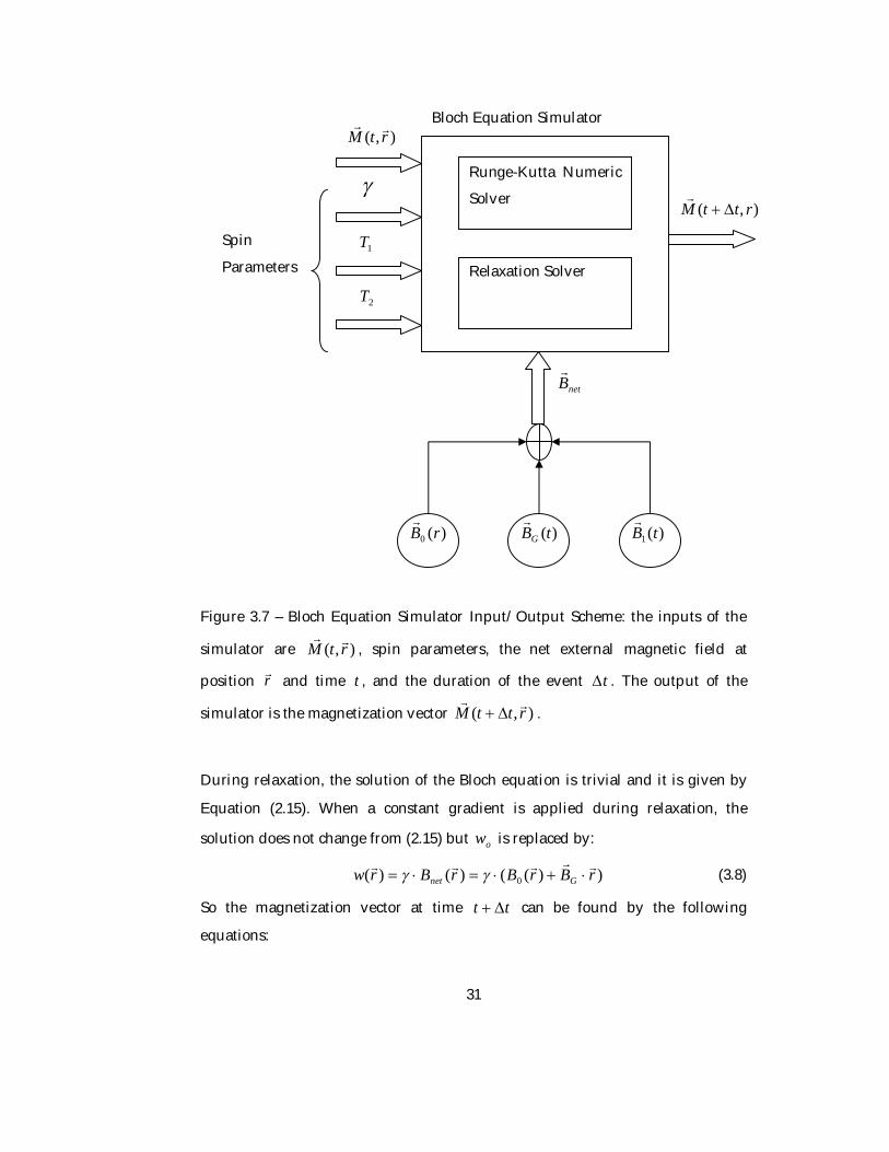
simulator is shown on Figure 3.7.
The inputs of the Bloch equation simulator are the magnetization vector ),( rtM
at position r , the spin parameters of this magnetization vector ( 21,, TT ), the net
external magnetic field at position r and time t and the duration of the event
t . The net external magnetic field is obtained from the summation of static
magnetic field, RF magnetic field and gradient fields. Static magnetic field 0B
only depends on spatial position, RF magnetic field only depends on time and the
gradient fields depend both on time and spatial position.
rrtBtBrBrtB Gnet ),()()(),( 10 (3.7)
The output of the simulator is the magnetization vector ),( rttM which is
calculated by using the input vector ),( rtM , the net external magnetic field and
spin parameters. The Bloch equation simulator is composed of two processing
blocks: one used for excitation and the other used for relaxation.
Page 44
31
Figure 3.7 – Bloch Equation Simulator Input/Output Scheme: the inputs of the
simulator are ),( rtM , spin parameters, the net external magnetic field at
position r and time t , and the duration of the event t . The output of the
simulator is the magnetization vector ),( rttM .
During relaxation, the solution of the Bloch equation is trivial and it is given by
Equation (2.15). When a constant gradient is applied during relaxation, the
solution does not change from (2.15) but ow is replaced by:
))(()()( 0 rBrBrBrw Gnet (3.8)
So the magnetization vector at time tt can be found by the following
equations:
),( rtM
1T
2T
Spin
Parameters
)(0 rB
)(1 tB
)(tBG
Runge-Kutta Numeric
Solver
Relaxation Solver
),( rttM
netB
Bloch Equation Simulator
Page 45
32
triwTt
xyxy eertMrttM
)(2),(),(
(3.9)
11 ),()1(),( 0 Tt
zT
t
zz ertMeMrttM
(3.10)
This equation is used in the relaxation solver block of Bloch equation simulator.
The simulator calculates the net external magnetic field using the spin position
r and the given time t by Equation (3.7). The result will be the summation of the
static magnetic field and the gradient field which is then used in Equation (3.8) to
calculate the precession frequency of the spin )(rw . Finally ),( rttM
is
determined according to Equations (3.9) and (3.10), and the whole calculation is
finished in one time step.
During excitation, the solution of Bloch equation gets more complicated. For a
rectangular shaped envelope function the Bloch equation has an analytical
solution for both on-resonance and off-resonance cases. But for an arbitrary
envelope function )(1 tB e , it is not possible to find a closed-loop analytic solution,
therefore numerical methods must be utilized. This is performed by the Runge-
Kutta solver of Bloch equation simulator.
Bloch equation is an ordinary differential equation which can be written in the
form of ),( yxfdtdy and 00 )( yxy . Considering Equation (2.6), the Bloch
equation is already in this form with 0)0( MM
. These type of differential
equations can be solved with numerical methods like Euler’s method, Mid-point
method and Runge-Kutta method. In this thesis the 4th order Runge-Kutta
method is preferred since it is the most used one in practice because of its high
accuracy and less computation time. The ode45() method in Matlab is the most
suggested method in numerical solvers package and this methods also
implements the 4th order Runge-Kutta method. The 4th order Runge-Kutta
method is a modified version of Euler’s method which uses 4 derivative values to
determine the value of the next point. The value of the function at the next step is
calculated as follows:
Page 46
33
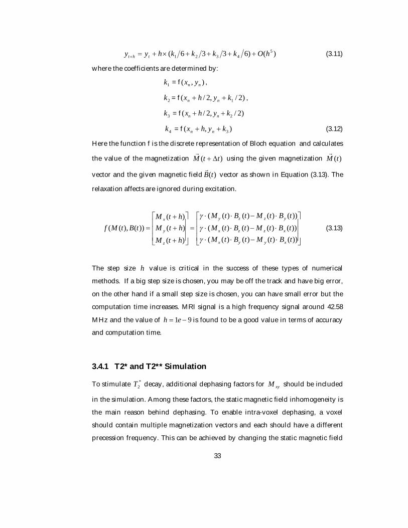
)()6336( 54321 hOkkkkhyy tht (3.11)
where the coefficients are determined by:
1k = f ),( nn yx ,
2k = f )2/,2/( 1kyhx nn ,
3k = f )2/,2/( 2kyhx nn
4k = f ),( 3kyhx nn (3.12)
Here the function f is the discrete representation of Bloch equation and calculates
the value of the magnetization )( ttM
using the given magnetization )(tM
vector and the given magnetic field )(tB
vector as shown in Equation (3.13). The
relaxation affects are ignored during excitation.
))()()()(())()()()(())()()()((
)()()(
))(),((tBtMtBtMtBtMtBtMtBtMtBtM
htMhtMhtM
tBtMf
xyyx
xzzx
yzzy
z
y
x
(3.13)
The step size h value is critical in the success of these types of numerical
methods. If a big step size is chosen, you may be off the track and have big error,
on the other hand if a small step size is chosen, you can have small error but the
computation time increases. MRI signal is a high frequency signal around 42.58
MHz and the value of 91 eh is found to be a good value in terms of accuracy
and computation time.
3.4.1 T2* and T2** Simulation
To stimulate *2T decay, additional dephasing factors for xyM should be included
in the simulation. Among these factors, the static magnetic field inhomogeneity is
the main reason behind dephasing. To enable intra-voxel dephasing, a voxel
should contain multiple magnetization vectors and each should have a different
precession frequency. This can be achieved by changing the static magnetic field
Page 47
34
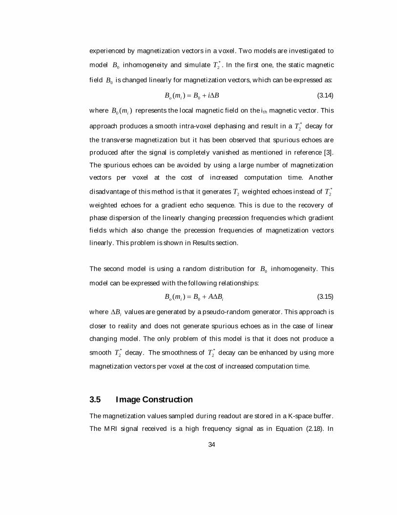
experienced by magnetization vectors in a voxel. Two models are investigated to
model 0B inhomogeneity and simulate *2T . In the first one, the static magnetic
field 0B is changed linearly for magnetization vectors, which can be expressed as:
BiBmB io 0)( (3.14)
where )(0 imB represents the local magnetic field on the ith magnetic vector. This
approach produces a smooth intra-voxel dephasing and result in a *2T decay for
the transverse magnetization but it has been observed that spurious echoes are
produced after the signal is completely vanished as mentioned in reference [3].
The spurious echoes can be avoided by using a large number of magnetization
vectors per voxel at the cost of increased computation time. Another
disadvantage of this method is that it generates 2T weighted echoes instead of *2T
weighted echoes for a gradient echo sequence. This is due to the recovery of
phase dispersion of the linearly changing precession frequencies which gradient
fields which also change the precession frequencies of magnetization vectors
linearly. This problem is shown in Results section.
The second model is using a random distribution for 0B inhomogeneity. This
model can be expressed with the following relationships:
iio BABmB 0)( (3.15)
where iB values are generated by a pseudo-random generator. This approach is
closer to reality and does not generate spurious echoes as in the case of linear
changing model. The only problem of this model is that it does not produce a
smooth *2T decay. The smoothness of *
2T decay can be enhanced by using more
magnetization vectors per voxel at the cost of increased computation time.
3.5 Image Construction
The magnetization values sampled during readout are stored in a K-space buffer.
The MRI signal received is a high frequency signal as in Equation (2.18). In
Page 48
35
practice, this signal is moved to baseband by a demodulation operation. In the
simulation, instead of a demodulator implementation, the static magnetic field 0B
is set to zero during readout. This operation removes the high frequency
resonance component from the signal and the baseband signal in Equation (2.19)
is obtained. The static magnetic field 0B is set to its previous value after readout.
K-space data is a complex data. The samples collected during readout are stored
in the K-space buffer as follows:
jnmSnmSnmKspace YX ),(),(),( (3.16)
where m is the mth phase encoding cycle and n is the nth sample collected in this
phase encoding cycle. As seen in Equation (3.15), the x component of transverse
magnetization xyM corresponds to the real part and the y component of
transverse magnetization corresponds to imaginary part of a k-space sample.
In order to obtain the image, simply a 2D inverse Fourier transform operation is
applied to the K-space buffer. The magnitude of the resultant matrix gives us the
parameter image function. Depending on the selected pulse sequence parameters,
the output image may be the proton density function, 1T function or 2T function
of the selected slice.
Page 49
36
CHAPTER 4
SIMULATION SOFTWARE ARCHITECTURE
AND USER INTERFACE
One of the motivations behind this study was to create an educational tool for
students and clinicians. For this aim, the simulation application is designed with
an educational perspective in terms of user interface and software design. The
simulation is composed of two applications. One is called “Spin simulator” and
the other is called “MRI Simulator”. The reason behind developing two
applications is to show all aspects of MRI as an imaging technique. The “MRI
Simulator” is the final product of this study and it generates images from 3D
virtual objects based on the pulse sequence parameters selected by the user. On
the other hand, the “Spin simulator” allows one to study NMR phenomenon by
applying excitation and relaxation events to a virtual object composed of one
voxel.
This chapter explains the software architecture and user interface of the
simulation software. The first section focuses on the software design of the
simulation in terms of java, applets and object oriented approach. The second
section explains the user interfaces of the applications in the simulation software.
Page 50
37
4.1 Software Architecture
Besides the aim of being an educational tool, this application also aims to be easily
accessible and practical for users. The most accessible environment in today’s
technology is the web environment. Therefore the applications of simulation are
developed as Java applets which are executed inside web browsers. Java applets
are java applications which run completely at the client side and can easily be
embedded into a web page. Most of the today’s popular web browsers support
java applets. So only an internet connection is needed to run this simulation.
Java is an object oriented, platform independent and high performance software
language. By its high level and well-organized APIs, it provides a fast and reliable
development environment for developers. With all these advantages, java became
a popular language for academic applications.
By use of the Java technology, the simulation software has been developed with
an object-oriented approach. The user interface components and the kernel of the
simulation are nicely separated. If desired, the simulation kernel easily be
integrated with another user interface. The user interface and the simulation
kernel run in separate tasks so that the user interface elements are accessible
when the simulation is running. This allows the simulation to be terminated
anytime.
The simulation kernel has been designed to be an MRI simulation framework
rather than a specific application code. Any pulse sequence type can easily be
realized in this framework using the following utility classes.
Page 51
38
Figure 4.1 – Utility classes to implement a pulse sequence
As shown in Figure 4.1, the cPulseSequence class holds a list of MRI events. By
AddMriEvent() method, relaxation or excitation can be added to the list to form a
series of events. The events in the list are processed consecutively by the Run()
method by calling the Process() method of each event in the list. With this
structure, any pulse sequence can easily be implemented and executed.
4.2 Application User Interfaces
The user interfaces of both applications have been designed to be interactive and
informative for the user. For this purpose, when a parameter is updated by the
user, the affected parameters are updated immediately by the application to
inform the user what that parameter affects.
4.2.1 Spin Simulator
The user interface of the “Spin simulator” application is shown in Figure 4.2.
Page 52
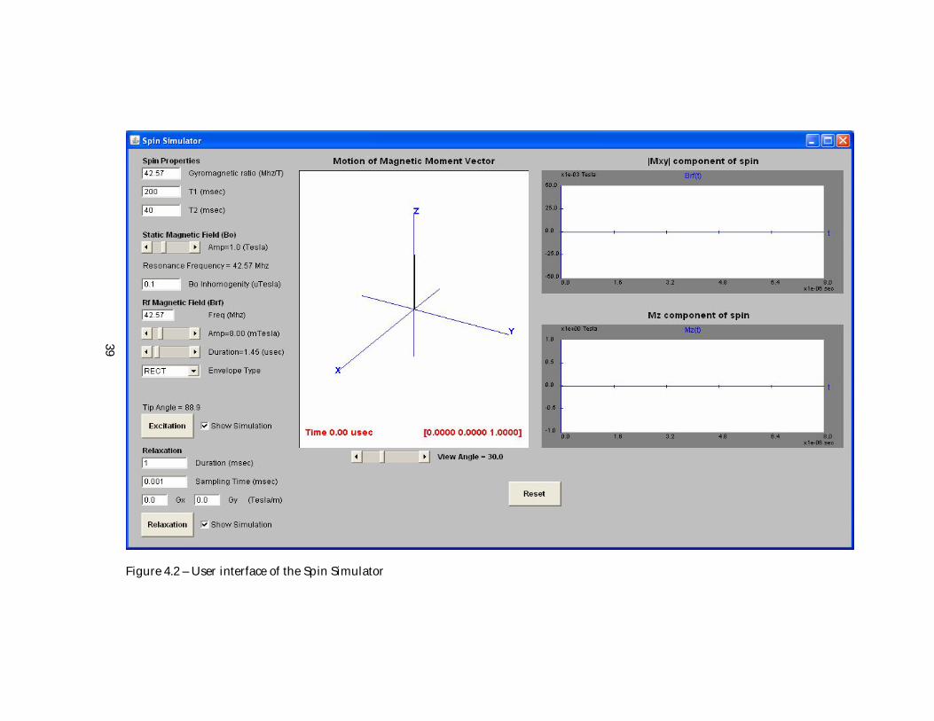
Figure 4.2 – User interface of the Spin Simulator
39
Page 53
40
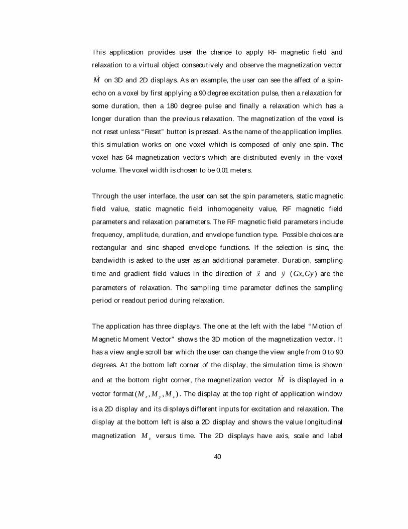
This application provides user the chance to apply RF magnetic field and
relaxation to a virtual object consecutively and observe the magnetization vector
M
on 3D and 2D displays. As an example, the user can see the affect of a spin-
echo on a voxel by first applying a 90 degree excitation pulse, then a relaxation for
some duration, then a 180 degree pulse and finally a relaxation which has a
longer duration than the previous relaxation. The magnetization of the voxel is
not reset unless “Reset” button is pressed. As the name of the application implies,
this simulation works on one voxel which is composed of only one spin. The
voxel has 64 magnetization vectors which are distributed evenly in the voxel
volume. The voxel width is chosen to be 0.01 meters.
Through the user interface, the user can set the spin parameters, static magnetic
field value, static magnetic field inhomogeneity value, RF magnetic field
parameters and relaxation parameters. The RF magnetic field parameters include
frequency, amplitude, duration, and envelope function type. Possible choices are
rectangular and sinc shaped envelope functions. If the selection is sinc, the
bandwidth is asked to the user as an additional parameter. Duration, sampling
time and gradient field values in the direction of x and y ( GyGx, ) are the
parameters of relaxation. The sampling time parameter defines the sampling
period or readout period during relaxation.
The application has three displays. The one at the left with the label “Motion of
Magnetic Moment Vector” shows the 3D motion of the magnetization vector. It
has a view angle scroll bar which the user can change the view angle from 0 to 90
degrees. At the bottom left corner of the display, the simulation time is shown
and at the bottom right corner, the magnetization vector M
is displayed in a
vector format ),,( zyx MMM . The display at the top right of application window
is a 2D display and its displays different inputs for excitation and relaxation. The
display at the bottom left is also a 2D display and shows the value longitudinal
magnetization zM versus time. The 2D displays have axis, scale and label
Page 54
41
information which provide the user, time information for the x coordinate and
unit information for the y coordinate.
The “Excitation” button starts an RF excitation to the magnetized virtual object
with the RF magnetic field parameters selected. The parameters are passed to the
simulation kernel at the instance the button is pressed. Thus changing the
parameters during the simulation will have no effect. The static magnetic field
and the static magnetic field inhomogeneity values are regarded when the
application is first invoked and get updated if the user changes these fields. A
change in static magnetic field value updates “Resonance Frequency” field’s
value. Before starting excitation, the user first configures the excitation
parameters by playing with slide bars and text boxes. As the user changes
amplitude and duration of the RF pulse, the tip angle field is updated with the
new tip angle value. If the selected envelope function is sinc, changes in
bandwidth field, also updates the tip angle. The tip angle is calculated according
to (2.10) if the envelope function type is rectangular. If the sinc shaped envelope
function is selected, the tip angle is calculated by the integration of the sinc
function over the excitation interval. The integration is performed using trapezoid
method. During excitation, the top right display shows the amplitude of RF
magnetic field amplitude versus time. This is shown in Figure 4.2. The 3D display
and 2D displays are updated at every 100 steps of the simulation kernel during
excitation. The Bloch equation simulator is configured with a step size of
102 eh for this application. Gradient field values are also taken into account
during excitation. If they are different than zero, it will be observed that the
flipped magnetization vector will have a phase dispersion.
The “Relaxation” button turns off the RF magnetic fields and starts a simulation
by relaxing the voxel for the specified duration with a step size equal to sampling
time field. The effect of gradient fields can be observed by setting the gradient
field values. During relaxation, the top right display shows the value of
Page 55
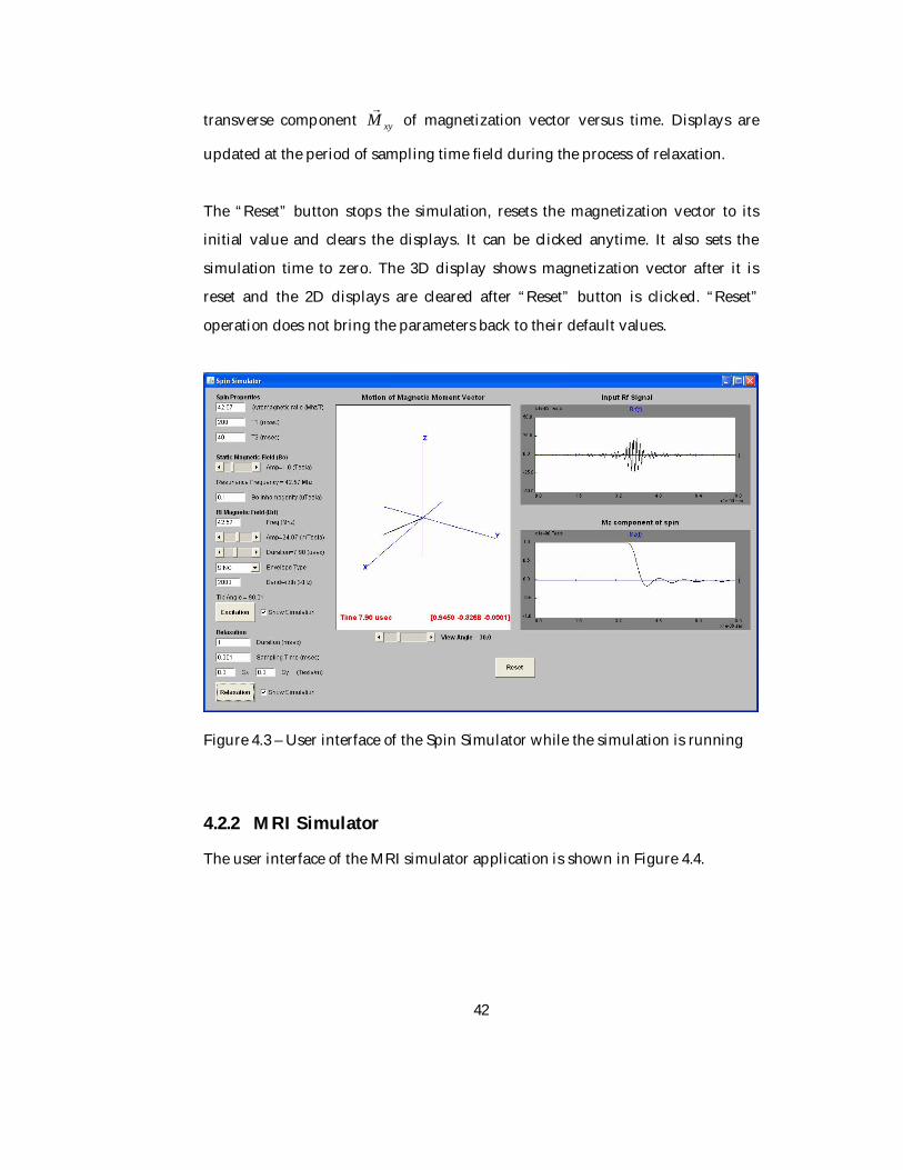
42
transverse component xyM
of magnetization vector versus time. Displays are
updated at the period of sampling time field during the process of relaxation.
The “Reset” button stops the simulation, resets the magnetization vector to its
initial value and clears the displays. It can be clicked anytime. It also sets the
simulation time to zero. The 3D display shows magnetization vector after it is
reset and the 2D displays are cleared after “Reset” button is clicked. “Reset”
operation does not bring the parameters back to their default values.
Figure 4.3 – User interface of the Spin Simulator while the simulation is running
4.2.2 MRI Simulator
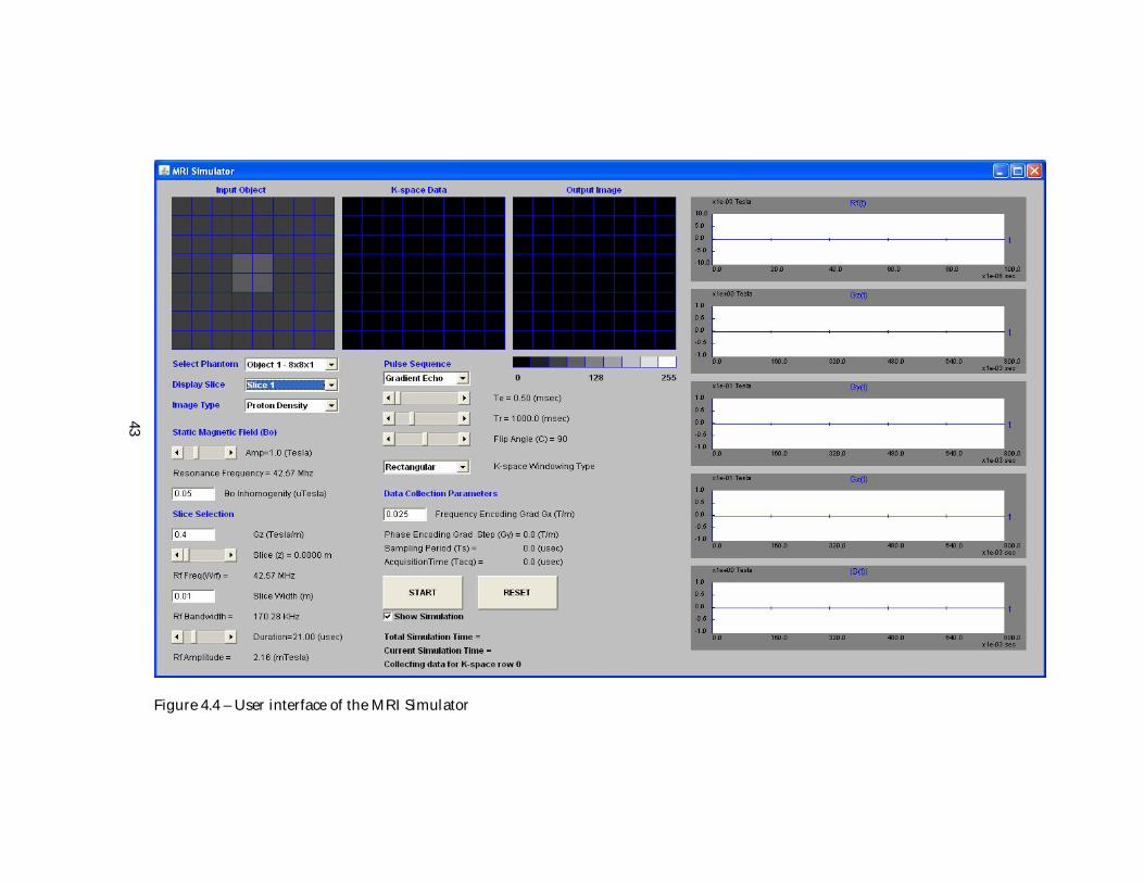
The user interface of the MRI simulator application is shown in Figure 4.4.
Page 56
Figure 4.4 – User interface of the MRI Simulator
43
Page 57
44
This application is the main output of this study. It allows the user to apply a
pulse sequence and slice selection pulse on a virtual 3D object and see the output
image. The user is able to select a 3D virtual object inside a set of predefined
virtual 3D objects.
As seen in Figure 4.4, the application does not have a menu and all the displays
and user interface elements are put into one window. On the upper left side, there
are 3 image displays showing the selected slice and parameter image of input
object, the k-space data and the output image respectively. On the right side of
the window, there are five 2D displays placed from top to bottom. These
windows show the change of RF signal versus time ( )(tRf ), gradient field change
along z direction versus time ( )(tGz ), gradient field change along y direction
versus time ( )(tGy ), gradient field change along x direction versus time ( )(tGx ),
and the magnitude of received signal versus time ( )(tS ) respectively. When the
application is started up, all the image displays and 2D displays are cleared
except the input object display. The application is simple to use. The user selects
an input image, configures the slice selection and pulse sequence parameters and
presses the “START” button to start the simulation. Except the input object
display, all the displays are updated during the simulation according to their
content. The user can stop the simulation anytime by pressing the “RESET”
button.
Below the input object display, there are three combo boxes which allow the user
to select an input object and to view the image of the selected parameter and
selected slice. Through the “Select Phantom” combo box, the user chooses the
virtual 3D input object which the simulation will be performed for. Each item of
the combo box shows the dimensions of the input object in the MxNxK format
where M is the number of voxels in x direction, N is the number of voxels in y
direction and K represents the number of slices. The parameter images of 3D
virtual objects are shown slice by slice. The slice selection is done with “Display
Page 58
45
slice” combo box. The number of items in the “Display slice” combo box is
updated according to the number of slices in the selected input object. The
selected slice is displayed in the input object display. MRI is capable of imaging
proton density, 1T and 2T maps of tissues. As explained before, each voxel in the
virtual object has proton density, 1T and 2T information. The third combo box
“Image Type” allows user to select which parameter image will be displayed.
The user can change the static magnetic field value using the “static magnetic
field” scroll bar. The resonance frequency field is updated as the static magnetic
field value is changed. The static magnetic field inhomogeneity value is the
inhomogeneity constant for oB distribution. The oB inhomogeneity distribution
is calculated each time a simulation is started .
In the slice selection part of the user interface, the user can configure the z
gradient zG , the slice center and the slice width. By changing the “Slice(z)” scroll
bar, the user chooses the center of the slice along the z direction. The height of a
virtual object is determined by the multiplication of number of slices and the
voxel width which is chosen as 0.01m. For a virtual object with 4 slices, the height
of the object will be 0.04 m. The slice center should not be above the object height
in order to receive signal from the object. The slice center determines the
frequency of the RF magnetic field according to the formula )( 0 czrf zGBw
where cz is the center of the slice and zG is the gradient field along z . The slice
width specifies the region around the slice center to be excited by the RF pulse
and determines the bandwidth of the RF pulse according to the formula
zGw z where z is the slice width. The slice width should also be selected
carefully considering that the voxel width is 0.01m. If the slice width is chosen a
value higher than voxel width, the output image becomes the addition of two
more slices. Besides these configurable parameters, there are RF pulse frequency,
RF pulse bandwidth, RF pulse duration and RF pulse amplitude fields in the slice
selection part. The values of these fields are calculated by the simulation software
and shown to the user when the “START” button is pressed.
Page 59
46
The pulse sequence part of the user interface provides to user to select a pulse
type and configure its parameters. The configurable parameters are time of echo
(TE), time of repetition (TR), and flip angle. TE and TR determine which
parameter of tissue will be weighted among proton density, 1T , and 2T . TE vale
cannot be chosen greater than TR.
The “K-space Windowing Type” field determines the type of windowing
operation to be applied on the k-space data. If “Rectangular” type is selected, no
windowing operation is applied. If Hamming is selected, a Hamming window is
applied to each row of k-space. As the name implies, the “Frequency Encoding
Grad Gx” field is used as the frequency encoding gradient value during pulse
sequence processing.
When the user press “START” button, the application takes the currently selected
input object, pulse sequence parameters, slice selection parameters, the k-space
windowing type and xG value, and performs the simulation using these settings.
Changing the parameters will not have any affect during the simulation. When
the simulation is started, firstly the simulation software calculates the data
collection parameters and displays them in the “data collection parameters” part
of the user interface. These parameters are phase encoding gradient step size,
sampling period used in readout, and total data acquisition time. The acquisition
time calculated as the number of samples taken in readout times the sampling
period. Also the total collection time is calculated as the number of phase
encoding steps times TR and written into the “Total Simulation Time” field.
There is a check box under “START” button called “Show Simulation”. If this
check box is not selected, the image displays and the 2D displays are not updated
during simulation. Only the “Current Simulation Time” and “Collecting Data for
K-space Row” fields are updated throughout the simulation. At the end of the
simulation, the k-space data and the output image are displayed. This mode
enables to obtain the output image in a shorter time. If the “Show Simulation”
Page 60
47
check box is selected, the 2D displays and the k-space image display are updated
during the simulation. This is shown in Figure 4.5. The 2D displays show the
current state of the magnetic inputs and the readout signal. During excitation, the
displays are updated every microsecond. For relaxation events, the displays are
updated before and after each event. The duration of the gradient fields
determine the width of the gradient pulses on the displays. The pulse widths are
calculated by dividing the duration of the gradient fields to 1 µsec. Since free
relaxation times are on the order of milliseconds, they cannot be drawn on 1
microsecond scale otherwise one phase encoding cycle does not fit into display
window. To overcome this problem, the free relaxation periods are shown with 50
pixels width on the displays. So the overall phase encoding cycle shown on the
displays is not to scale. The 2D displays are updated every 1 µsec except free
relaxation (no gradient field applied) times. The K-space data display shows
which point of k-space is being filled during readout. This is performed by
blinking the pixel of k-space which is being filled and then setting it to its value.
After all the k-space is filled, the output image display is updated with the output
image.
Figure 4.5 – User interface of the MRI Simulator while simulation is running
Page 61
48
The “RESET” button stops the simulation, sets the virtual object to its initial state
and clears the displays except the input object display. It can be clicked anytime.
It also sets the simulation time to zero. “RESET” operation does not bring the
parameters back to their initial values.
Page 62
49
CHAPTER 5
SIMULATION RESULTS AND DISCUSSION
The first simulation program “Spin Simulator” allows the user to observe the
NMR phenomenon with different excitation and relaxation parameters on a
voxel. The second program “MRI Simulator” generates MRI images from a virtual
3D object by using the pulse sequence and slice selection parameters provided by
the user. In this chapter, outputs of experiments from both applications are
presented and compared with the expected results.
The results for the “Spin Simulator” application are classified according to
specific NMR situations. The results for “MRI Simulator” contain MRI image
outputs for different slice selection and pulse sequence parameters.
5.1 Results from Spin Simulator
The virtual object used in the “Spin Simulator” program is a voxel whose
structure is defined in section 3.1. The voxel is represented by 64 magnetization
vectors. The voxel has only one spin whose parameters are given by the user. The
default spin parameters and proton density are chosen as 57.42 MHz/Tesla,
2001 T msec , 402 T msec and, proton density p =1.0 and these values are
used for the experiments presented here.
Page 63
50
5.1.1 Resonance
This experiment is performed with the following parameters: 0.10 B Tesla, a
rectangular shaped RF pulse with frequency 57.42rff MHz, amplitude = 8.1
mTesla, and duration = 1.45 µsec which creates a 90 pulse.
Figure 5.1 – On-Resonance excitation: Bo = 1.0 Tesla, a rectangular shaped RF
pulse with frequency 42.57 MHz, amplitude = 8.1 mTesla, and duration = 1.45
µsec.
As seen in Figure 5.1, the magnetization vector was tilted away from z axis by
the 90 pulse as expected. To verify the accuracy of the numerical method
(Runge-Kutta 4th order) used in the solution of Bloch equation, the Bloch equation
has been solved by the Matlab’s ode45 () method which uses also uses a Runge-
Kutta implementation for solution of ordinary differential equations. Matlab
simulation gave the same result for the magnetization vector [-0.9891 -0.1471
0.0001]. This result has also been compared with the analytic solution which
produced the result of [-0.9891 -0.1471 0.0000]. The slight difference between the
Page 64
51
analytic and numerical solution is due to 1T relaxation which is ignored in the
analytic solution.
It should also be noted that the simulation program uses a step size of 102 eh
in the Runge-Kutta solution which tracked the analytic solution successfully.
When the step size is taken as 91 eh , the simulation produces the result of [-
0.9857 -0.1569 0.0014] which deviates from the real solution slightly. Decreasing
h increases the accuracy but also increases the simulation time by )( 3nO . To find
out how much deviation occurs from the exact solution by increasing h , a 180
pulse is applied to the system with frequency 57.42rff MHz, amplitude = 8.1
mTesla, and duration = 2.90 µsec with 91 eh . The simulator produces the
result [-0.0196 -0.0058 -0.9961] in this case. It is observed that the step size value
can be taken as 91 eh by sacrificing a %.004 error in the z component of
magnetization vector.
To see what happens when the envelope function is not rectangular, the system is
excited with a sinc shaped RF pulse with frequency 57.42rff MHz, amplitude
= 24.07 mTesla, duration = 7.90 µsec and bandwidth = 2000 KHz which
corresponds to 90 pulse. The excitation signal )(1 tB
and the evolution of the z
component of magnetization vector can be seen in the figure below.
Page 65
52
Figure 5.2 – On-Resonance excitation with sinc shaped envelope function:
frequency 42.57 MHz, amplitude = 24.07 mTesla, duration = 7.90 µsec and
bandwidth = 2000 KHz.
As seen in Figure 5.2, during the side lobes of )(1 tB
, )(tM
keeps its equilibrium
value. During the main lobe, )(tM
moves to transverse plane quicker compared
to rectangular pulse excitation (Figure 5.1). After the main lobe, a small
fluctuation around xy plane is observed. It is interesting to observe that the side
lobes of sinc pulse has little affect on the magnetization vector.
Page 66
53
5.1.2 Off-Resonance
To observe the off-resonance case, the object is excited with the following
parameters: 0.10 B Tesla, a rectangular shaped RF pulse with frequency
87.42rff MHz, amplitude = 8.1 mTesla, and duration = 1.45 µsec which would
be a 90 pulse if it were an on-resonance excitation. The output of the simulator is
shown in the figure below.
Figure 5.3 – Off-Resonance excitation, w small: performed with frequency
87.42rff MHz, amplitude = 8.1 mTesla, and duration = 1.45 µsec. The left
display shows how much the magnetization vector tipped on the yz plane.
Although the excitation frequency is 0.30 MHz apart from resonance frequency,
the magnetization vector )(tM
still tilts into the transverse plane by a significant
amount. This is expected as explained in Equation (2.12).
If the excitation frequency is selected further away from resonance frequency,
)(tM
moves away from z axis slightly as shown in Figure 5.4. The following
Page 67
54
result is obtained by application of a rectangular shaped RF pulse with frequency
17.43rff MHz, amplitude = 8.1 mTesla, and duration = 2.90 µsec which would
cause a 180 pulse if it were an on-resonance excitation. The 0.60 MHz deviation
form resonance frequency resulted in almost no transverse magnetization for spin
system.
Figure 5.4 – Off-Resonance excitation, w big: performed with with frequency
17.43rff MHz, amplitude = 8.1 mTesla, and duration = 2.90 µsec. The left
display shows how much the magnetization vector tipped on the yz plane.
5.1.3 Relaxation
In all the relaxation results presented below, the system is first excited with a 90
rectangular pulse with the following parameters: frequency 57.42rff MHz,
amplitude = 8.1 mTesla, and duration = 1.45 µsec. Then samples are taken from
the spin system for different scenarios.
Page 68
55
5.1.3.1 T1 and T2 Relaxation
If the static magnetic field oB was homogenous, then all the magnetization
vectors in the object would be rotating with the same precession frequency and
the net transverse magnetization vector would be decaying with 2T . To illustrate
this, the oB inhomogeneity constant is set to 0 for this experiment and the system
is put into relaxation with a sampling period of 0.2 msec for 40 msec which equals
to 2T constant of the spin.
Figure 5.5 – 2T relaxation for 40 msec with a sampling period of 0.2 msec.
As seen in Figure 5.5, the transverse magnetization vector loses %63 of its
magnitude after 40 msec relaxation as expected.
To show 1T relaxation, the system is relaxed for 200 msec which equals to 1T
constant of the spin and samples are taken at 0.5 msec intervals. The gradient
fields are set to zero in both cases. This is shown on the figure below together
with the transverse magnetization xyM change.
Page 69
56
Figure 5.6 – 1T and 2T relaxation: the top display shows )(tM xy vs. t and presents
2T relaxation, the bottom display shows )(tM z vs. t and presents 1T relaxation.
The system is relaxed for 200 msec. with a sampling period of 0.5 msec.
As seen on Figure 5.6, the longitudinal magnetization zM gains %63 of its
magnitude after a relaxation of 200 msec. which is the 1T constant of the system.
The transverse magnetization xyM vanishes after 200 msec relaxation as expected.
As observed, the transverse magnetization diminishes early before the
longitudinal magnetization is recovered.
Page 70
57
5.1.3.2 T2* Relaxation
During relaxation, the individual magnetic moments in a voxel have different
precession frequencies because of 0B inhomogeneity. To create this
inhomogenity, the 0B inhomogeneity value is set to 0.1 µTesla. As a result of this
inhomogeneity, each magnetization vector in the voxel will have a different
precession frequency determined by Equation (3.15). This is illustrated in the
figure below.
Figure 5.7 – The phase dispersion of magnetic moment vectors with time: the top-
right display shows the distribution of magnetization vectors at 0.25th msec, the
top right display shows the distribution at 1.50th msec, the bottom left display
shows the distribution at 2.75th msec and the bottom right display shows the
distribution at 4.0th msec.
Page 71
58
Figure 5.7 contains four snapshots taken from the simulation program at different
times. The first snapshot is taken after 0.250 msec with a sampling rate of 0.01
msec. Then the system is relaxed for 1.250 msec more and the second snapshot is
taken. The third snapshot is taken after 1.250 msec from the second snapshot. The
fourth snapshot is taken after another 1.250 msec of relaxation which makes a
total of 4.0 msec relaxation.
The voxel is composed of 64 magnetization vectors. So the total magnetization
vector will be composed of 64 different precession frequencies. This is shown in
Figure 5.7 by displaying each of them with a separate color. As time progresses,
the phase difference between magnetization vectors increases and this causes the
transverse magnetization vector xyM to decay at a rate of *2T instead of 2T . This
is shown in the figure below where the system is relaxed for 40 msec with a
sampling interval of 0.1 msec.
Figure 5.8 – The decay of )(tM xy vs. t with *2T when B =0.1 µTesla: the system
is relaxed for 40 msec with a sampling interval of 0.1 msec.
As seen in Figure 5.8, the magnitude of transverse magnetization vector vanishes
after 5 msec which should normally vanish after two 2T intervals. In a normal
Page 72
59
MRI system, the transverse magnetization decays exponentially at a rate of *2T .
Physically, there are millions of magnetization vectors in a voxel and this leads to
an exponential decay for net transverse magnetization. But in the simulation, a
voxel is represented by only 64 magnetization vectors because of computation
issues and the phase dispersion of these magnetization vectors create side lobes
after the main decay which is not seen in reality. If more magnetization vectors
are used to represent a voxel, the decay function approaches to an exponential
decay.
Another thing that should be underlined is that the 0B inhomogeneity value
determines the rate of decay. This is shown in Figure 5.9 where the 0B
inhomogeneity value is set to 0.2 µTesla and the system is relaxed for 40 msec
with a sampling rate of 0.1 msec.
Figure 5.9 – The decay of )(tM xy vs. t with *2T with B =0.2 µTesla: the system is
relaxed for 40 msec with a sampling rate of 0.1 msec.
As seen in Figure 5.9, the transverse magnetization decays at a faster rate
compared to Figure 5.8. The first zero crossing of xyM occurs at 2.5 msec in this
Page 73
60
case where it occurs at 5.0 msec when the 0B inhomogeneity value is set to 0.1
µTesla.
5.1.4 Echo Generation
Echo generation is the key step of MRI process. In this part, two methods of echo
generation spin echo and gradient echo are presented.
5.1.4.1 Spin Echo
To generate a spin echo, first the system is excited with a rectangular shaped RF
pulse with frequency 57.42rff MHz, amplitude = 8.1 mTesla, and duration =
1.45 µsec which corresponds a 90 pulse. The 0B inhomogeneity value is set to 0.2
µTesla. After the excitation, the system is relaxed for 5 msec with a sampling rate
of 0.1 msec. The transverse magnetization vanishes after this relaxation due to *2T
decay. After this a 180 pulse is applied to recover the phase dispersion. The
parameters of the 180 pulse are as follows: frequency 57.42rff MHz,
amplitude = 16.2 mTesla, and duration = 1.45 µsec. Finally the system is relaxed
for duration of 10 msec in which an echo is generated at the 10th msec. Figure 5.9
shows the phase recovery of magnetization vectors just before the echo
generation. This relaxation - 180 pulse - relaxation sequence is called a spin echo
sequence. This sequence is applied to the system two times which generates the
two echoes shown in Figure 5.10.
Page 74
61
Figure 5.10 –Phase recovery after 180 pulse: the left display shows the
distribution of magnetization vectors at time instance 9.0 msec and the right
display shows the distribution of magnetization vectors at time instance 9.9 msec
just before the echo generation.
As seen in Figure 5.10, the phase dispersion decreases as approaching to the echo
time. The 180 pulse maintains the phase total coherence between magnetization
vectors and causes echo generation.
Figure 5.11 – Spin echo simulation: performed with a sequence of 5 msec relation -
180 pulse - 10 msec relaxation-180 pulse – 10 msec relaxation. Two echoes are
observed at time instances 10 msec and 20 msec.
Page 75
62
As seen in Figure 5.11, the peaks of echoes are at 10 msec and 20 msec as
expected. The time instants where the 180 pulses are applied can be observed by
the abrupt change of phase at 5 msec and 15 msec. If this sequence is applied
many times consecutively, it is observed that the peaks of the echoes follow the
exponential decay of magnetization vector with 2T . This is shown in Figure 5.12
where the 180 pulse - relaxation sequence is applied four times after an intial
relaxation with an echo time of 8 msec.
Figure 5.12 – Spin echoes following 2T decay: performed with a sequence of 180
pulse - 8 msec relaxation applied 4 times after an initial relaxation of 4 msec.
5.1.4.2 Gradient Echo
Gradient echoes are generated by spoiling the transverse magnetization with a
gradient field and recovering it with another gradient field. To generate a
gradient echo, first the system is excited with a rectangular shaped RF pulse with
frequency 57.42rff MHz, amplitude = 8.1 mTesla, and duration = 1.45 µsec
which corresponds a 90 pulse. The 0B inhomogeneity value is set to 0.1 µTesla.
After the 90 pulse, the system is relaxed for 0.050 msec with a sampling time of
0.001 msec and Gx gradient field set to 0.1. After this 0.050 msec relaxation, the Gx
gradient value is set to -0.1 Tesla/m and the system is put into relaxation for
Page 76
63
duration of 0.100 msec sampled at an interval 0.001 msec. The phase dispersion
and recovery of magnetization vectors and, the change of transverse
magnetization )(tM xy for this sequence are shown in Figure 5.13 and 5.14,
respectively.
Figure 5.13 –Phase dispersion and recovery of magnetization vector during
gradient echo: the left display shows the dispersion of magnetization vectors at 50
µsec and the right display shows the recovery of magnetization vectors at time
instance 100 µsec.
The left side of Figure 5.13 shows the magnetization vectors after the positive
gradient is applied for 0.050 msec. As seen in the figure, the precession
frequencies of 64 magnetization vectors are grouped into 8 frequencies since the
gradient field is applied only in x direction. If Gy gradient is applied together
with Gx gradient, then 64 different frequencies are observed. The right display
shows the phase recovery of magnetization vectors after the negative gradient is
applied for 0.050 msec. At this point the net phase dispersion created by the
gradient fields is zero. The small phase dispersion between magnetization vectors
at this instant is caused by 0B inhomogeneity.
Page 77
64
Figure 5.14 – Gradient echo simulation: a relaxation of 50 µsec is applied with
Gx=0.1 Tesla/m and followed by a relaxation of 50 µsec with Gx=-0.1 Tesla/m.
As seen in Figure 5.14, the first positive gradient (Gx=0.1) applied vanishes the
net transverse magnetization xyM in a very short duration (0.050 msec). The
negative gradient (Gx=-0.1) applied for the same duration recovers the phase
dispersion and an echo is obtained with a peak value at the 100th µsec.
An interesting behavior for the gradient echo is observed when the 0B
inhomogeneity has a linearly changing distribution instead of a random
distribution. The system is excited with a rectangular shaped RF pulse with
frequency 57.42rff MHz, amplitude = 8.1 mTesla, and duration = 1.45 µsec
which corresponds a 90 pulse. The 0B inhomogeneity value is set to 0.1 µTesla.
After the 90 pulse, the system is put into relaxation for 2 msec sampled at 0.01
msec with the gradient fields off. Then the system is relaxed for 0.050 msec with a
sampling time of 0.001 msec and Gx gradient field set to 0.1. After this, the Gx
gradient value is set to -0.1 Tesla/m and the system is put into relaxation for a
duration of 0.100 msec sampled at an interval 0.001 msec. The transverse
magnetization )(tM xy during this sequence is shown in Figure 5.15.
Page 78
65
Figure 5.15 – Gradient echoes following 2T : the figure shows a gradient echo after
a relaxation of 1 msec. The gradient echo is obtained with a relaxation of 0.050
msec with Gx=0.1 Tesla/m followed by a relaxation of same duration with Gx=-
0.1. Bo inhomogenity has a linear changing distribution. The peak of the echo
follows 2T decay instead of *2T decay.
As seen in Figure 5.15, the first relaxation with gradient fields off is a normal *2T
decay because of the 0B inhomogeneity. After this, the positive gradient applied
causes the net magnetization to diminish as expected. The negative gradient
following the positive one recovers the phase coherence and generates the echo
which is expected to follow *2T decay. But it is seen that the peak of the echo
follows 2T decay instead of *2T decay. It is understood that the negative gradient
field also recovers the phase dispersion caused by 0B inhomogeneity. The reason
for this is found out to be the linear change of 0B field among magnetization
vectors. Since the precession frequencies of magnetization vectors has a linear
change, a gradient field re-phases the spins since the gradient field also creates a
linear change in precession frequencies of magnetization vectors. The linearly
changing 0B field creates a smooth *2T decay but it has the drawback of being
neutralized by a gradient field applied in the opposite direction of 0B field
change. This disables the peaks of gradient echoes to follow a *2T decay.
Page 79
66
To overcome this problem, the 0B magnetic field inhomogeneity should be
modeled with a random distribution. If the same experiment is carried out with a
random 0B inhomogeneity distribution, the following result in Figure 5.16 is
obtained. The parameters and the sequence are same with the previous
experiment except that the positive gradient followed by a negative gradient is
continued with another positive gradient of 0.100 msec to obtain a second
gradient echo.
Figure 5.16 – Gradient echoes following *2T : the figure shows two gradient echoes
after a relaxation of 1.5 msec. The gradient echoes are obtained with a relaxation
of 0.050 msec with Gx=0.1 Tesla/m followed by a relaxation of 0.100 msec
duration with Gx=-0.1 Tesla/m and another relaxation of 0.100 msec with Gx=0.1
Tesla/m. 0B inhomogenity has a random changing distribution and the
inhomogeneity constant is set to 0.1. The peak of the echo follows *2T decay as
expected.
As seen in Figure 5.16, the peak values of the two echoes follow *2T decay as
expected. These results show that a random 0B inhomogeneity distribution
should be used in order to simulate gradient echoes correctly.
Page 80
67
5.2 Results from MRI Simulator
The experiments presented here are the simulation results of predefined 3D
virtual phantoms with different pulse sequences and varying parameters. There
four virtual objects in the application selectable by the user. The table below lists
the specifications of each object.
OBJECTS Proton
Density
T1 (msec) T2 (msec)
Tissue-1
(Background)
60 500 40 Object 1 –
8 x 8 x 1
Slice 1
Tissue-2 90 50 80
Tissue-1
(Background)
20 200 40 Slice 1
Tissue-2 100 200 40
Tissue-1
(Background)
20 200 40 Slice 2
Tissue-2 100 200 40
Tissue-1
(Background)
20 200 40 Slice 3
Tissue-2 100 200 40
Tissue-1
(Background)
20 200 40
Object 2 –
8 x 8 x 4
Slice 4
Tissue-2 100 200 40
Tissue-1
(Background)
20 200 40 Object 3 –
16 x 16 x 2
Slice 1
Tissue 2 100 200 40
Page 81
68
Tissue-1
(Background)
20 200 40 Slice 2
Tissue-2 100 200 40
Tissue-1
(Background)
20 200 40
Tissue-2 100 200 40
Tissue-3 100 200 40
Tissue-4 20 200 40
Object 4 –
32 x 32 x 1
Slice 1
Tissue-5 100 200 40
Figure 5.17 –Input objects specification
The table in Figure 5.17 lists the proton density, 1T and, 2T values of the tissues in
the slices of the input objects. The dimension information of each is object is
specified with their titles. The first tissue of each slice corresponds to the
background tissue. These objects are displayed on the “MRI Simulator”
application slice by slice using a 256 level gray scale color scheme.
Each of these four objects are created for different purposes. The first object is a
8x8x1 object which has a non-uniform 1T and 2T map. This single slice object
allows the user to obtain 1T weighted and 2T weighted images by adjusting the
pulse sequence parameters appropriately. All parameter (proton density, 1T , 2T )
maps of this object has a higher square shaped density over a uniform
background. So the k-space data of the output images should a sinc function
which is the Fourier transform of rectangular window.
Page 82
69
The second object is an 8x8x4 with all slices having a uniform 1T and 2T map.
This object can be used to test the performance of the slice selection pulse. All the
slices of this object have square shaped higher density regions and these regions
are placed at different positions among slices so that contributions from other
slices at the output image can easily be noticed.
The third object is a 16x16x2 object. The first slice of this object is designed to
observe chemical-shift affect. For this purpose, the shielding factor of the voxels of
the high proton density tissue in the first slice, is set to a value of 0.999990 which
corresponds to 10 parts per million. If this slice is imaged with any pulse
sequence type, the affect of chemical shift should be seen as a shift at the output
image.
The fourth object is a simplified version of Shepp-Logan phantom. It is a 32x32x1
object with different elliptic tissues.
5.2.1 Slice Selection
The second phantom which has four slices is used to perform slice selection pulse
with different parameters. In the simulation, sinc function is used as the envelope
function of the excitation pulse. The sinc function should be applied infinitely to
create a perfect slice selection profile. Since this is not realizable, the sinc pulse
should be packed with as many side lobes as possible to create a nice slice
selection profile. So the RF duration selection is critical for slice selection
performance. The 0B inhomogeneity value is set to 0.0 for slice selection tests to
get rid of imperfections resulting from 0B inhomogeneity and to focus only on
slice selection. The first experiment aims to select the first slice of the virtual object
and is performed with the following parameters:
Pulse sequence parameters: {Gradient Echo, TE = 0.50 msec, TR = 1000 msec, Flip
Angle = 90 }, Slice selection parameters: {Gz = 0.4 Tesla/m, Slice Center = 0.00 m,
Page 83
70
Slice Width = 0.01 m, Rf Duration = 21 µsec}. The 0B inhomogeneity value is set
to 0.
Figure 5.18 – Slice selection, one slice: The top display shows the gradient echo
result for the second phantom. The selected slice of the input object, the k-space
collected and the output object are shown from left to right. The bottom display
shows the RF pulse used in the slice selection. Pulse sequence parameters:
{Gradient Echo, TE = 0.50 msec, TR = 1000 msec, Flip Angle = 90 }, Slice selection
parameters: {Gz = 0.4 Tesla/m, Slice Center = 0.00 m, Slice Width = 0.01 m, Rf
Duration = 21 µsec}. The Bo inhomogeneity value is set to 0.
As seen in Figure 5.18, the output image is very close to the first slice as desired
but the contribution from the second slice is noticeable. Figure 5.18 also shows the
RF pulse used in the slice selection. As seen on the diagram, the sinc function has
only one side lobe on each side. If the RF duration is made shorter, the selectivity
of the RF pulse decreases and contributions from other slices increase.
Page 84
71
The center of the slice and the width of the slice determine which region of the 3D
object to be excited. If the previous simulation is repeated by only changing the
slice center to 0.005 m which is the middle of the first and the second slice, the
result in Figure 5.19 is obtained. The whole configuration parameters for this
simulation are as follows:
Pulse sequence parameters: {Gradient Echo, TE = 0.50 msec, TR = 1000 msec, Flip
Angle = 90 }, Slice selection parameters: {Gz = 0.4 Tesla/m, Slice Center = 0.005
m, Slice Width = 0.01 m, Rf Duration = 21 µsec}. The 0B inhomogeneity value is
set to 0.
Figure 5.19 – Slice selection, middle of two slices is selected: the display shows the
gradient echo result for the second phantom, the middle of the first two slices is
selected as the slice center. Data from both slices exist at the output image. Pulse
sequence parameters: {Gradient Echo, TE = 0.50 msec, TR = 1000 msec, Flip Angle
= 90 }, Slice selection parameters: {Gz = 0.4 Tesla/m/m, Slice Center = 0.005 m,
Slice Width = 0.01 m, Rf Duration = 21 µsec}. The 0B inhomogeneity value is set
to 0.
As seen in Figure 5.19, the output image is the addition of the first two slices. The
excitation pulse designed to select the middle of the two slices excited both the
slices the same amount, and the output image is formed by equal contribution of
both slices.
Page 85
72
If a hard pulse is applied to the object with the following configuration, the
output image in Figure 5.20 is obtained. To apply a hard pulse to the system, the
z gradient Gz is set to 0. This makes the bandwidth of the sinc pulse 0 which
converts the sinc to pulse to a rectangular function.
Pulse sequence parameters: {Gradient Echo, TE = 0.50 msec, TR = 1000 msec, Flip
Angle = 90 }, Slice selection parameters: {Gz = 0.0 Tesla/m, Slice Center = 0.00 m,
Slice Width = 0.01 m, Rf Duration = 4 µsec}. The 0B inhomogeneity is set to 0.
Figure 5.20 – Slice selection with a hard pulse: The top display shows the gradient
echo result for the second phantom. The selected slice of the input object, the k-
space collected and the output object are shown from left to right. The bottom
display shows the hard RF pulse used in the slice selection. Pulse sequence
parameters: {Gradient Echo, TE = 0.50 msec, TR = 1000 msec, Flip Angle = 90 },
Slice selection parameters: {Gz = 0.0 Tesla/m, Slice Center = 0.00 m, Slice Width =
0.01 m, Rf Duration = 4 µsec}. The 0B inhomogeneity value is set to 0.
As seen in Figure 5.20, the output image is the addition of four slices. The
background intensity of the output image is 4 times the background of one slice
Page 86
73
as expected. The RF pulse is also shown in Figure 5.20 which is an unmodulated
sinusoidal.
5.2.2 Spin Echo
Spin echo is a widely used pulse sequence type because of its ability to generate
2T weighted images. The first result presented here is obtained for the first
phantom which has a single slice. The pulse parameters are adjusted for a proton
density image by selecting TE a low value and TR a high value. The parameters
used for this experiment are as follows:
Pulse sequence parameters: {Spin Echo, TE = 0.50 msec, TR = 2500 msec, Flip
Angle = 90 }, Slice selection parameters: {Gz = 0.4 Tesla/m, Slice Center = 0.00 m,
Slice Width = 0.01 m, Rf Duration = 21 µsec}. The 0B inhomogeneity value is set
to 0.1.
Figure 5.21 – Spin echo result for the first phantom, proton density weighted:
Pulse sequence parameters: {Spin Echo, TE = 0.50 msec, TR = 2500 msec, Flip
Angle = 90 }, Slice selection parameters: {Gz = 0.4 Tesla/m, Slice Center = 0.00 m,
Slice Width = 0.01 m, Rf Duration = 21 µsec}. The Bo inhomogeneity value is set to
0.1 .
As seen in Figure 5.21, the k-space data is sinc function as expected and the
output image is the same as input image with a small intensity difference. The
Page 87
74
peak of the k-space data is at the center as expected, which equals the sum of
proton densities of voxels in the object.
To obtain 2T weighted images, TR should be chosen long and TE value should be
chosen carefully to differentiate between tissues. The first object has a 2T map
with two tissues whose values are 40 msec and 120 msec respectively. To weight
the output image with 2T values of these two tissues, a TE value which will
suppress the signal coming from one of the tissues should be selected. TE is
selected 100 msec for this purpose and the following simulation is performed
with the configuration below.
Pulse sequence parameters: {Spin Echo, TE = 100 msec, TR = 2500 msec, Flip
Angle = 90 }, Slice selection parameters: {Gz = 0.4 Tesla/m, Slice Center = 0.00 m,
Slice Width = 0.01 m, Rf Duration = 21 µsec}. The 0B inhomogeneity value is set
to 0.1.
Figure 5.22 – Spin echo result for the first phantom, 2T weighted: Pulse sequence
parameters: {Spin Echo, TE = 100 msec, TR = 2500 msec, Flip Angle = 90 }, Slice
selection parameters: {Gz = 0.4 Tesla/m, Slice Center = 0.00 m, Slice Width = 0.01
m, Rf Duration = 21 µsec}. The 0B inhomogeneity value is set to 0.1.
As seen in the figure above, the output image is 2T weighted instead of proton
density. Since the 2T image of the object has a rectangular shape, the k-space data
Page 88
75
is a sinc function. Another thing that should be remarked is that the intensity of
the 2T weighted image is the weighted image of the proton density map. There is
a big intensity difference between the input image and the output image in the
figure above. Because the input object display shows the 2T map which is
displayed according to the 2T values of the image. On the other hand, the
intensity of the output image is a 2T weighted version of the proton density
image.
The next simulation presents a spin echo result for the second phantom which is a
multi-slice object. An unexpected artifact is observed in spin echo simulations for
multi-slice objects. The configuration parameters for the simulation are as shown
below:
Pulse sequence parameters: {Spin Echo, TE = 100 msec, TR = 1000 msec, Flip
Angle = 90 }, Slice selection parameters: {Gz = 0.4 Tesla/m, Slice Center = 0.01 m,
Slice Width = 0.01 m, Rf Duration = 21 µsec}. The 0B inhomogeneity value is set
to 0.1.
Figure 5.23 – Spin echo result for the second phantom, second slice selected: An
unexpected bright line is observed at the most left column of k-space which
causes a distortion at the top row of output image. Pulse sequence parameters: {
Spin Echo, TE = 100 msec, TR = 1000 msec, Flip Angle = 90 }, Slice selection
parameters: {Gz = 0.4 Tesla/m, Slice Center = 0.01 m, Slice Width = 0.01 m, Rf
Duration = 21 µsec}. The 0B inhomogeneity value is set to 0.1.
Page 89
76
As seen in Figure 5.23, the most left column of k-space is filled with a high value
unexpectedly. The rest of the k-space data is like a sinc function as expected . This
high frequency line in k-space creates a varying line at the first row of the output
image. This unexpected result is not seen for single slice objects or for gradient
simulations of multi-slice objects. By checking the magnetization values of all the
voxels in the virtual object during simulation, it is found out that this artifact is
caused by the neighbor slice. In spin echo, one 90 pulse and one 180 pulse is
applied to the virtual object for each phase encoding step. Because of the
imperfection of slice selection pulse, the 90 pulse creates a small amount of
transverse magnetization in the neighbor slice, the 180 pulse increases this
transverse magnetization and creates this artifact.
5.2.3 Gradient Echo
Gradient echo has the ability to generate 2T * weighted images. The first result
presented here is obtained for the second phantom with 0B inhomogeneity value
set to 0. In this case, the magnetization vectors will decay with 2T and gradient
echo is expected to produce the same result with spin echo. The pulse sequence
parameters are adjusted for proton density weighting, the whole configuration for
this experiment is as follows:
Pulse sequence parameters: {Gradient Echo, TE = 0.50 msec, TR = 1000 msec, Flip
Angle = 90 }, Slice selection parameters: {Gz = 0.4 Tesla/m, Slice Center = 0.02 m,
Slice Width = 0.01 m, Rf Duration = 21 µsec}. The 0B inhomogeneity value is set
to 0.
Page 90
77
Figure 5.24 – Gradient echo result for the second phantom, third slice selected:
Pulse sequence parameters: {Gradient Echo, TE = 0.50 msec, TR = 1000 msec, Flip
Angle = 90 }, Slice selection parameters: {Gz = 0.4 Tesla/m, Slice Center = 0.02 m,
Slice Width = 0.01 m, Rf Duration = 21 µsec}. The Bo inhomogeneity value is set to
0. The input object display shows the first slice of the object.
As seen in the figure above, the output image generated by the simulation is
perfectly equal to the selected slice.
The next simulation presents a gradient echo result for the third phantom with an
inhomogeneous 0B . The configuration for this experiment is as follows:
Pulse sequence parameters: {Gradient Echo, TE = 0.50 msec, TR = 1000 msec, Flip
Angle = 90 }, Slice selection parameters: {Gz = 0.4 Tesla/m, Slice Center = 0.02 m,
Slice Width = 0.01 m, Rf Duration = 21 µsec}. The 0B inhomogeneity value is set
to 0.1.
Page 91
78
Figure 5.25 – Gradient echo result for the third phantom, first slice selected: Pulse
sequence parameters: {Gradient Echo, TE = 0.50 msec, TR = 1000 msec, Flip Angle
= 90 }, Slice selection parameters: {Gz = 0.4 Tesla/m, Slice Center = 0.02 m, Slice
Width = 0.01 m, Rf Duration = 21 µsec}. The Bo inhomogeneity value is set to 0.
The Figure 5.25 shows the k-space data and output image for this simulation. The
output image reflects the selected slice and a small contribution from the second
slice.
5.2.4 Echo Planar
Echo planar pulse sequence is a fast MR imaging method. Echo planar imaging
may have different k-space trajectories. The one implemented in this thesis uses a
rectilinear k-space trajectory. Since there is only one excitation in echo planar
imaging, it is the also the fastest pulse sequence in the simulation. An echo planar
experiment is performed for the fourth object with the following configuration.
Pulse sequence parameters: {Gradient Echo, TE = 0.50 msec, TR = 1000 msec, Flip
Angle = 90 }, Slice selection parameters: {Gz = 0.4 Tesla/m, Slice Center = 0.00 m,
Slice Width = 0.01 m, Rf Duration = 21 µsec}. The 0B inhomogeneity value is set
to 0.
Page 92
79
Figure 5.26 – Echo planar result for the fourth phantom with a homogenous 0B :
Pulse sequence parameters: {Gradient Echo, TE = 0.50 msec, TR = 1000 msec, Flip
Angle = 90 }, Slice selection parameters: {Gz = 0.4 Tesla/m, Slice Center = 0.00 m,
Slice Width = 0.01 m, Rf Duration = 21 µsec}. The Bo inhomogeneity value is set to
0.
As seen in Figure 5.26, the output image is the same with input image as
expected. The same experiment is repeated by setting 0B inhomogeneity to 0.02
µTesla. The output of the simulator in this case is shown in Figure 5.27.
Figure 5.27 – Echo planar result for the fourth phantom with 0B inhomogeneity
equal to 0.02: Pulse sequence parameters: {Gradient Echo, TE = 0.50 msec, TR =
1000 msec, Flip Angle = 90 }, Slice selection parameters: {Gz = 0.4 Tesla/m, Slice
Center = 0.00 m, Slice Width = 0.01 m, Rf Duration = 21 µsec}.
Page 93
80
As seen in the figure above, including 0B inhomogeneity in the simulation
generated degradation in the image compared to homogenous 0B case. The
degradation in the image increases further with increasing inhomogeneity
constant.
5.2.5 MRI Artifacts
The simulation program has the ability to generate many of the artifacts in MRI.
These artifacts can be counted as 0B inhomogeneity, slice selection imperfection,
Gibbs ringing artifact, aliasing and chemical –shift affect. Some of these artifacts
are shown in the previous results.
A common artifact in MRI is aliasing which occurs when the k-space sampling
parameters are not selected according to the Nyquist theorem. The result shown
in Figure 5.28 presents such a case. It is obtained with the following configuration
of the application.
Pulse sequence parameters: {Echo Planar, TE = 0.50 msec, TR = 1000 msec, Flip
Angle = 90 }, Slice selection parameters: {Gz = 0.4 Tesla/m, Slice Center = 0.00 m,
Slice Width = 0.01 m, Rf Duration = 21 µsec}. The 0B inhomogeneity value is set
to 0. Frequency encoding gradient Gx is set to 0.1 Tesla/m.
Page 94
81
Figure 5.28 – Echo planar result for the fourth phantom with aliasing: Pulse
sequence parameters: {Echo Planar, TE = 0.50 msec, TR = 1000 msec, Flip Angle =
90 }, Slice selection parameters: {Gz = 0.4 Tesla/m, Slice Center = 0.00 m, Slice
Width = 0.01 m, Rf Duration = 21 µsec}, Gx = 0.1 Tesla/m, the Bo inhomogeneity
value is set to 0.
As seen in Figure 5.28, the output image is the addition of shifted, inverted
portions of input image.
Another artifact in MRI arises from the change in resonance frequency of the spin
due to the chemical environment around the nucleus called chemical-shift affect.
To observe the chemical-shift affect, a simulation is performed with the
configuration below for the third object which is specially prepared for this
experiment.
Pulse sequence parameters: {Echo Planar, TE = 0.50 msec, TR = 1000 msec, Flip
Angle = 90 }, Slice selection parameters: {Gz = 0.4 Tesla/m, Slice Center = 0.00 m,
Slice Width = 0.01 m, Rf Duration = 21 µsec}. The 0B inhomogeneity value is set
to 0.
Page 95
82
Figure 5.29 – Echo planar result for the third phantom, chemical-shift affect:
Pulse sequence parameters: {Echo Planar, TE = 0.50 msec, TR = 1000 msec, Flip
Angle = 90 }, Slice selection parameters: {Gz = 0.4 Tesla/m, Slice Center = 0.00 m,
Slice Width = 0.01 m, Rf Duration = 21 µsec}. The Bo inhomogeneity is set to 0.
As seen in Figure 5.29, the output image is a 1 pixel upwards shifted version of
the input image.
The Gibbs ringing artifact occurs due to the finite sampling in k-space. It appears
as a ringing artifact around sharp changing borders. In the simulation, a
noticeable ringing affect could not be observed. To avoid this artifact, windowing
of k-space data is performed at the expense of spatial resolution loss. The “MRI
Simulator” application allows two types of windowing: rectangular and
hamming. The next simulation result shows how the output image is affected if
Hamming window is selected.
Page 96
83
Figure 5.30 – Echo planar result for the fourth phantom, Hamming window
applied: The output image is a blurred version of the input image. Pulse sequence
parameters: {Echo Planar, TE = 0.50 msec, TR = 1000 msec, Flip Angle = 90}, Slice
selection parameters: {Gz = 0.4 Tesla/m, Slice Center = 0.00 m, Slice Width = 0.01
m, Rf Duration = 21 µsec}. The Bo inhomogeneity value is set to 0.0 µTesla.
As seen in the figure above, the Hamming windowing operation caused
resolution loss and blurring at the output image .
Page 97
84
CHAPTER 6
CONCLUSION
6.1 Summary of the Thesis
In this thesis, a realistic and web accessible MRI simulator based on the solution
of Bloch equation is proposed and implemented. The simulator generates images
from virtually defined 3D objects using the pulse sequence and slice selection
parameters provided by the user. The simulation is implemented in Java and the
application is developed as a Java applet which is accessible through a web page.
The simulation software is composed of two applications: “Spin Simulator” and
“MRI Simulator”. The “Spin Simulator” allows one to observe NMR phenomenon
on 3D and 2D displays by applying RF pulse and relaxation to a virtual object and
is developed as an educational and supportive tool for “MRI Simulator”. Gradient
echo and spin echo and echo planar pulse sequences are implemented. The “MRI
Simulator” generates slice images by executing the pulse sequence with the
selected parameters on the 3D virtual object. The applications are designed with
an interactive and educative user interface.
6.2 Discussions and Future Work
The simulation kernel is based on the solution of Bloch equation. Bloch equation
is solved by numerical methods during excitation. This enables to see the effect of
an arbitrary envelope function on a spin system. If the analytic solution were used
instead of numerical methods, the output signal transmitted by the virtual object
Page 98
85
would be the summation of magnetization vectors only in the selected slice. The
numerical solution is executed on the entire volume of the 3D object and
contributions from other slices are also taken into account so that a more realistic
signal is received form the object. During relaxation, the analytic solution of Bloch
equation is used to calculate the magnetization values. Solving the Bloch equation
by numerical methods during excitation and using the analytical solution during
relaxation provides a realistic and efficient way of implementing the simulation
kernel.
The 3D virtual object definition is structured in a rich content and is flexible to
represent a real object by its all features. The structure allows one voxel to be
composed of multiple magnetization vectors which may produce more realistic
magnetization data at the cost of increased simulation time. The structure also
allows more than one voxel to be placed at the same spatial position. This enables
chemical shift affect to be observed during simulation.
In this thesis, two models for static magnetic field inhomogeneity are
investigated. These are a random distributed noise model and a linear changing
model. The effectiveness and problems of both models are observed. Including
the static magnetic field inhomogeneity in the simulation, causes the individual
magnetization vectors to have different precession frequencies during relaxation
which enables the *2T affect to be simulated successfully. Since the magnetization
vectors have position information and are distributed evenly on the entire volume
of the object, the gradient fields change the precession frequencies of the
individual magnetization vectors. This enables the **2T affect to be observed.
Simulating *2T and **
2T affects successfully is essential for successful
implementation of gradient echo and spin echo pulse sequences. As shown in the
results section, spin echoes and gradient can be generated as in the physical case.
Since the 3D virtual object is a discrete representation of a real object, the *2T and
**2T decay curves are not exponentials as in the real case. This is due the
representation of millions of spins with a couple of thousand spins at most. If
Page 99
86
higher number of magnetization vectors are used to represent the virtual object,
more realistic *2T and **
2T decays are obtained. Comparing both static magnetic
field inhomogeneity models, the linear changing produces a smoother *2T decay
with a less number of magnetization vectors but has the problem of being
recoverable by gradient fields. On the other hand, the noise model is more
realistic but more magnetization vectors should be used to obtain smooth *2T
decay which increases computation time.
The simulation does not take into account the magnetic susceptibility variations
among tissues which is one of the reasons behind *2T decay. In future, this affect
can also be included in the simulation by changing the magnetic susceptibility of
the spins on the borders of the tissues.
Developing the application in a platform independent and object oriented
language like Java, shortened the development time and created a modular and
expandable application. The simulation kernel is totally separable from the user
interface of the application and is designed like a framework for MRI simulation
applications. In MRI, there are many types of pulse sequences. In this thesis, the
gradient echo, spin echo and echo planar pulse sequences are implemented. But it
is very easy to implement any type of pulse sequence by use of the object oriented
structure mentioned in section 4.1.
The simulation of a spin echo sequence for a 8x8x3 object takes 1 minute on an
Intel Core Duo CPU at 1.73 GHZ and 2 GB RAM computer. The high simulation
time is due to the small step size of the Runge-Kutta method used in the solution
of Bloch equation. To decrease the simulation time, an adaptive step size
algorithm can be embedded into the current implementation which can decrease
the number of steps in a run. But if bigger objects (like 256x256x3) are used in the
simulation, the simulations will still take long durations. To avoid this, parallel
processing can be applied by distributing the kernel of the simulation to many
nodes.
Page 100
87
The simulator allows three types of pulse sequences to be selected. To give the
user the flexibility to try any type of pulse sequence, the user interface can be
designed to allow the user to create different pulse sequences. This can be done
by defining excitation and relaxation events and putting them in a sequential
order. The same idea can be applied to virtual object definitions. The simulation
uses pre-defined virtual objects, in the future this can be replaced by a user
interface that allows the user to set the proton density and spin parameters of 3D
virtual object.
An MRI simulation can be extended to include the simulation of several actors in
MR imaging process. As part of this study, the NMR phenomena and the imaging
process of MR systems are simulated in a realistic way. The following items
which are not simulated as part of this study, can also be included in an MRI
simulation to produce more realistic simulations.
RF magnetic field inhomogeneity
Gradient fields with rising and falling edges
Magnetic susceptibility variation on the borders of tissues
Receiver coil inhomogeneity
As a conclusion, an easily accessible and helpful tool for MRI related people has
been developed as a result of this study. It has the simulation capabilities of
previous MRI simulators in an effective way and adds the advantage of being a
web based and educative tool.
Page 101
88
REFERENCES
[1] Zhi-Pei Liang, Paul C. Lauterbur, “Principles Of Magnetic Resonance
Imaging/A Signal Processing Perspective” IEEE Press, New York
[2] The Basics of MRI, http://www.cis.rit.edu/htbooks/mri , visited on 31 July
2008
[3] D.A. Yoder, E. Changchien, C.B. Paschal, J.M. Fitzpatrick, “MRI simulator
with static field inhomogeneity,” SPIE Medical Imaging, 4684, 592–603, 2002.
[4] H. Benoit-Cattin, G. Collewet, B. Belaroussi, H. Saint-Jalmes, C. Odet, “The
SIMRI Project: a versatile and interactive MRI Simulator,” Journal of Magnetic
Resonance, 173, 97-115, 2005.
[5] S. Kwan, A.C. Evans, G.B. Pike, An extensible MRI simulator for post-
processing evaluation, in: International Conference on Visualization in
Biomedical Computing, VBC 96, 1996, pp. 135–140.
[6] A.R. Brenner, J. Kursch, T.G. Noll, Distributed large-scale simulation of
magnetic resonance imaging, Magnetic Resonance Materials in Biology, Physics,
and Medicine 5 (1997) 129–138.
[7] G. Torheim, P.A. Rinck, R.A. Jones, J. Kvaerness, A simulator for teaching MR
image contrast behavior, MAGMA 2 (1994) 515–522.
[8] T. Hacklaender, C. Schalla, A. Truemper, H. Mertens, J. Hiltner, B.M. Cramer,
A virtual MR scanner for education, RSNA 2002, 88th Scientific Assembly and
Annual Meeting, Radiology (2002) 757–225.