arX

iv:2

006.

0465

9v1

[q-

fin.

PR]

8 J

un 2

020

Explicit option valuation in the exponential NIG model

Jean-Philippe Aguilar ∗

June 08, 2020

Abstract

We provide closed-form pricing formulas for a wide variety of path-independent options, in the

exponential Lévy model driven by the Normal inverse Gaussian process. The results are obtained in

both the symmetric and asymmetric model, and take the form of simple and quickly convergent series,

under some condition involving the log-forward moneyness and the maturity of instruments. Proofs are

based on a factorized representation in the Mellin space for the price of an arbitrary path-independent

payoff, and on tools from complex analysis. The validity of the results is assessed thanks to several

comparisons with standard numerical methods (Fourier-related inversion, Monte-Carlo simulations) for

realistic sets of parameters. Precise bounds for the convergence speed and the truncation error are also

provided.

Keywords: Lévy Process; Normal inverse Gaussian Process; Stochastic Volatility; Option Pricing.

AMS subject classifications (MSC 2020): 60E07, 60E10, 60H35, 65C30, 65T50, 91G20, 91G30.

JEL Classifications: C00, C02, G10, G13.

∗BRED Banque Populaire, 18 Quai de la Râpée, FR-75012 Paris, Email: jean-philippe.aguilar@bred.fr

1 Introduction

Whether the dramatic COVID-19 events and the subsequent turmoils in global markets were unpredictable

"black swan" events in the sense of Taleb (2010) or, on the contrary, could have been forecasted (or at

least, following the terminology of Giannone & al. (2008), "nowcasted") will undoubtedly be the matter

of intense debates. But what is already certain is that they demonstrate, yet again, that the kurtosis in

the distribution of asset returns far exceeds the tails of the Normal one, and that market volatility is not

constant over time; it should therefore be a minimal requirement for any reliable market model that they

include (at least) these two stylized facts.

It has now long been known that exponential - sometimes also called geometrical - Lévy models fulfil

these conditions. Such models have been introduced in quantitative finance during the late 1990s / early

2000s in several influential works, and make the assumption that asset log returns are driven by some

drifted Lévy process: a Normal inverse Gaussian (NIG) process in Barndorff-Nielsen (1995, 1997), a

Variance Gamma (VG) process in Madan et al. (1998), a hyperbolic or a generalized hyperbolic process

in Eberlein and Keller (1995); Eberlein (2001), a CGMY process in Carr & al. (2002) or a stable (or α-

stable) process in Mittnik & Rachev (2000); Carr and Wu (2003). Stable distributions, in particular, may

be noted for their historical importance, having been considered a credible candidate for the modelling of

asset prices as early as in the 1960s by Mandelbrot (1963) in the context of the cotton market, thus paving

the way to the more generic setup of exponential Lévy models. Readers who may be less familiar with

the broad family of Lévy processes and their applications to finance are invited to refer to the classical

references Bertoin (1996); Schoutens (20003); Cont & Tankov (2004); Rachev et al. (2011).

In the present work, we will be particularly interested in the class of exponential Lévy models whose

Lévy process is distributed according to a NIG distribution, namely, the class of exponential NIG models.

NIG distributions were originally introduced for physical purpose, more precisely to model the complex

behavior of dunes and beach sands, in the seminal article Barndorff-Nielsen (1977); as noted above, they

have subsequently been introduced for financial purpose approximately two decades later, because they

feature several degrees of freedom that have a direct empirical interpretation in terms of financial time

series. First, they possess fat tails, allowing for the presence of extreme variations of prices (positive or

negative jumps); when the tail parameter goes to infinity, then the NIG distribution degenerates into the

Normal distribution and the exponential NIG model recovers the Black-Scholes model (Black & Scholes

(1973)). Second, NIG distributions can be skewed, allowing to capture the asymmetry that can be observed

1

in the distribution of jumps (price drops occurring more often that raises). Last, but not least, a NIG

process can be interpreted as a drifted Brownian motion whose time follows an inverse Gamma process

- this is a consequence of the fact that the NIG distribution is actually a particular case of a so-called

Normal variance-mean mixture, the mixing distribution being the inverse Gaussian (IG) distribution; the

NIG process is therefore a time changed Lévy process, which allows for stochastic volatility modelling and

related phenomena, such as clustering or negative correlation between the returns and their volatility (see

details in Carr and Wu (2004)).

Of course, since it was introduced, the exponential NIG model has been proved to provide a very

good fitting to financial data many times. Let us mention, among others, initial tests for daily returns

on Danish and German markets in Barndorff-Nielsen (1995); Rydberg (1997) and subsequently on the

FTSE All-share index (also known as "Actuaries index") in Venter & de Jongh (2002). More recently, the

impact of high frequency trading has also been taken into account, and calibrations have been performed

on intraday returns e.g. in Figueroa-López et al. (2012) for different sampling frequencies. Let us also

mention that multivariate extensions of the exponential NIG model, i.e., featuring a different time change

for different assets, have also been considered (see Luciano & Semeraro (2010) and references therein).

As one could expect, pricing contingent claims turns out to be a tougher task in the exponential

NIG model than it is in the usual Black-Scholes framework. Numerical methods are largely favored,

including Monte-Carlo valuation methods (Ribeiro and Webber (2003)), numerical evaluation of Fourier

(Lewis (2001)) and Fast Fourier (Carr & Madan (1999)) transforms. The success of Fourier transform

methods is strongly linked to the relative simplicity of the characteristic function of most exponential

Lévy models, and has opened the way to a wide range of other transform based approaches: they include,

among others, the COS method by Fang & Osterlee (2008), the Hilbert transform method (see notably

a recent application to time-changed Lévy processes in Zeng and Kwok (2014)) or the local basis Frame

PROJection (PROJ) method by Kirkby (2015). Efforts have also been made towards analytic evaluation or

approximations: in Ivanov (2013), a closed-form formula (in terms of Appel functions) for the European

call is derived in the particular case where the NIG distribution has a tail parameter of 1/2, and in

Albrecher & Predota (2004) approximations and bounds are provided for Asian options.

In this paper, we would like to show that it is actually possible to obtain tractable closed-form pricing

formulas in the exponential NIG model, for a broad range of path independent instruments. This is

made possible by a remarkable property allowing to express the Mellin transform of an arbitrary path

independent option as the product of the Mellin transforms of its payoff and of the NIG probability

2

density. Inverting it by means of residue summation yields the option price, computed under the form of

quick convergent residue series whose terms are directly expressed in terms of the model’s parameters. This

Mellin residue summation method has been used very recently within the framework of other exponential

Lévy models, namely in the Finite Moment Log Stable (FMLS) model in Aguilar & Korbel (2019) and in

the exponential VG model in Aguilar (2020); in the present paper, we will therefore demonstrate that the

technique is also well-suited to the exponential NIG model. Moreover, we will establish pricing formulas

for both the symmetric and the asymmetric NIG processes, while the formulas in the VG case in Aguilar

(2020) were mainly obtained for the symmetric VG process. Due to the nature of the residues series,

however, we will need to introduce a restriction on the model parameters to ensure the convergence to the

price. We will show that this condition is compliant with most of the implied parameters calibrated in the

literature; moreover, when options are not far from the money, it is automatically satisfied.

The paper is organized as follows: in section 2, we start by recalling fundamental concepts on the NIG

process and its implementation via exponential Lévy models. In section 3, we focus on the symmetric

NIG process: after establishing the pricing formula in the Mellin space for an arbitrary path independent

instrument, we evaluate, analytically, the price of the European and digital options, as well as payoffs

featuring more exotic attributes (power options, log contracts, . . . ). In section 4 we extend the pricing

formula to the more general case of the asymmetric model, and provide analytic formulas for the digital and

European prices. In section 5, precise bounds for the convergence speed and the truncation errors of the

series are obtained, and the validity of the results is assessed by comparing them with classic numerical

methods (Fourier inversion, Monte Carlo simulations). For the reader’s convenience, the paper is also

equipped with two appendices: in appendix A we provide a short overview of the Mellin transform, and

in appendix B we recall some important special function identities that are used throughout the paper.

2 Model definition

In this section we recall important concepts on NIG distributions and processes; more details can be

found in the initial articles by Barndorff-Nielsen or in subsequent review articles like Hanssen & Øigård

(2001); Papantolen (2008). We also introduce the exponential NIG model, following the classical setup of

exponential Lévy models such as defined e.g. in Schoutens (20003); Tankov (2010).

3

2.1 The Normal inverse Gaussian process

The Normal inverse Gaussian (NIG) process can be defined by in several different ways: as a process

following a NIG distribution, in terms of its Lévy measure, or as a time-changeed Lévy process.

NIG density The NIG distribution, denoted by NIG(α, β, δ, µ), is four-parameter distribution whose

density function is:

f(x) :=αδ

πeδ√α2−β2+β(x−µ)

K1

(

α√

δ2 + (x− µ)2)

√

δ2 + (x− µ)2. (1)

The function z → K1(z) is the modified Bessel function of the second kind and of index 1 (sometimes

also called Macdonald function, see definitions and properties in appendix B). α > 0 is a tail or steepness

parameter controlling the kurtosis of the distribution; the large α regime gives birth to light tails, while

small α corresponds to heavier tails. β ∈ (−α,α − 1) is the skewness parameter: β < 0 (resp. β > 0)

implies that the distribution is skewed to the left (resp. the right), and β = 0 that the distribution is

symmetric around the location parameter µ ∈ R. δ > 0 is the scale parameter and plays an analogue role

to the variance term σ2 in the Normal distribution; when β = 0, the Normal distribution is itself recovered

in the large steepness regime:

NIG(α, 0, δ, µ) −→α→∞

N (µ, σ2) , σ2 :=δ

α. (2)

We say that a stochastic process Xtt≥0 is a NIG process if it has NIG distributed increments, that

is if Xt+h − Xt ∼ NIG(α, β, δh, µh) for all h ≥ 0; it follows from (1) that the density of the process

conditionally to X0 = 0 is (with a slight abuse of notations):

f(x, t) :=αδt

πeδt

√α2−β2+β(x−µt)

K1

(

α√

(δt)2 + (x− µt)2)

√

(δt)2 + (x− µt)2. (3)

It is also possible to define the NIG process as time-changed drifted Brownian motion: if Itt≥0 is a

process distributed according to an Inverse Gamma density of shape δ√

α2 − β2 and mean rate 1 and if

Wt≥0 is a standard Wiener process, then the process

Xt = βδ2 It + δWIt (4)

is a centered NIG process (µ = 0). The process Itt≥0 is a tempered stable subordinator; it has positive

4

jumps, and therefore is interpreted as a business time that can differ from the operational time, the

occurence of jumps corresponding to periods of intense business activity. A similar interpretation holds

for instance in the case of the Variance Gamma process, which features another example of tempered

stable subordination (via a Gamma process).

Lévy symbol The NIG process is a (pure jump) Lévy process whose characteristic function Ψ(u, t) :=

E[eiuXt ] can be written down as Ψ(u, t) = etψ(u), where the characteristic exponent, or Lévy symbol, is

known in exact form:

ψ(u) := log Ψ(u, 1) = iµu − δ(

√

α2 − (β + iu)2 −√

α2 − β2)

. (5)

The process admits the Lévy-Khintchine triplet (a, 0, ν(dx)), where the drift a and the Lévy measure ν

are defined by

a := µ +2αδ

π

1∫

0

sinh(βx)K1(αx) dx

ν(dx) :=αδ

πeβx

K1(α|x|)|x| dx,

(6)

allowing to write down the characteristic exponent (5) in terms of its Lévy-Khintchine representation:

ψ(u) = iau +

∫

R

(eiux − 1− iux1|x|<1) ν(dx). (7)

Let us observe that it follows from the definition of the Lévy measure ν that the NIG process has infinite

variation and infinite intensity (i.e. ν(R) = ∞), and therefore possesses a very rich dynamics with infinite

number of jumps on any time interval - this is why no Brownian component is even needed in the Lévy-

Khintchine triplet. We should also note that the NIG process has all its moments finite, which is not the

case with (double-sided) α-stable processes for instance: this is because the Bessel function admits the

asymptotic behavior (see (142))

K1(|x|) ∼|x|→∞

√

π

2|x| e−|x|, (8)

and therefore the tails of the NIG measure ν are less heavy than the tails of the α-stable measure (which

has polynomial decrease in 1/|x|1+α). In other words, the jumps in the NIG process are not as big as for

α-stable processes, but allow finiteness of moments and therefore of option prices; in the α-stable case,

this would be achieved only for spectrally negative processes (i.e., having negative jumps only).

5

2.2 The exponential NIG model

Model specification Let T > 0 and S : t ∈ [0, T ] → St be the market price of some financial asset,

seen as the realization of a time dependent random variable Stt∈[0,T ] on the canonical space Ω = R+

equipped with its natural filtration. We assume that there exists a risk-neutral measure Q under which

the instantaneous variations of St can be written down as:

dStSt

= (r − q) dt + dXt (9)

where r ≥ 0 is the risk-free interest rate and q ≥ 0 is the dividend yield (both assumed to be deterministic

and continuously compounded), and where Xtt∈[0,T ] is the NIG process. The solution to the stochastic

differential equation (9) it the exponential process

ST = St e(r−q+ω)τ +Xτ , ω := −ψ(−i), (10)

where τ := T − t is the time horizon and ω is the martingale adjustment (also called convexity adjust-

ment, or compensator) determined by the martingale condition EQ[ST |St] = e(r−q)τSt; it follows from the

definition of the Lévy symbol (5) that this adjustment is equal to:

ω = −µ + δ(

√

α2 − (β + 1)2 −√

α2 − β2)

. (11)

It is interesting to note that, in the large steepness regime, (11) has the following asymptotic behavior:

ω ∼α→∞

−µ − σ2

2(1 + 2β) , σ2 :=

δ

α. (12)

Taking µ = 0 (centered process) and β = 0 (symmetric process), (12) recovers the the Gaussian martingale

adjustment −σ2/2, and the exponential NIG model (9) degenerates into the Black-Scholes model.

Contingent claim valuation Given a path-independent payoff function P, i.e., a positive function

depending only on the terminal value ST of the market price and on some strike parameters K1, . . . ,KN >

0, then the value at time t of a contingent claim delivering a payoff P at maturity is equal to the following

risk-neutral expectation:

C = EQ[

e−rτP(ST ,K1, . . . ,Kn) |St]

. (13)

6

The conditional expectation (13) can be achieved by integrating all possible realizations for the payoff over

the probability density of the NIG process, thus resulting in:

C = e−rτ+∞∫

−∞

P(St e(r−q+ω)τ + x,K1, . . . ,Kn) f(x, τ) dx. (14)

3 Option pricing in the symmetric model

In this section, we assume that β = 0, i.e., that the process Xtt∈[0,T ] in (9) is distributed according to

the symmetric distribution NIG(α, 0, δt, µt). First, we establish a general pricing formula for an arbitrary

path independent instrument; then, we apply this formula to the analytic evaluation of several options

and contracts.

3.1 Pricing formula

Let us start by establishing a representation for the symmetric NIG density f(x, t) under the form of a

Mellin-Barnes integal.

Lemma 3.1. For any c1 ∈ R+, the following holds true:

f(x, t) =α

2πeαδt

c1+i∞∫

c1−i∞

Γ(s12

)

K1− s12(αδt)

(

2δt

α

)

s12

|x− µt|−s1 ds12iπ

. (15)

Proof. Taking β = 0 in (3) yields:

f(x, t) =αδt

πeαδt

K1

(

α√

(δt)2 + (x− µt)2)

√

(δt)2 + (x− µt)2. (16)

Using the Mellin transform for the Bessel function (see table 7 in appendix A with ν = 1) and the Mellin

inversion formula (125), we can write:

K1

(

α√

(δt)2 + (x− µt)2)

√

(δt)2 + (x− µt)2=

1

2δτ

c1+i∞∫

c1−i∞

Γ(s12

)

K1− s12(αδτ)

(

2δt

α

)

s12

|x− µt|−s1 ds12iπ

(17)

for any c1 > 0. Inserting into (16) yields the representation (15).

7

Let us now introduce the double-sided Mellin transform of the payoff function:

P ∗(s1) =

∞∫

−∞

P(

Ste(r−q+ω)τ+x,K1, . . . ,Kn

)

|x− µτ |−s1 dx (18)

and assume that it exists for Re(s1) ∈ (c−, c+) for some real numbers c− < c+. Then, as a consequence

of the risk-neutral pricing formula (14) and of lemma 3.1, we immediately obtain:

Proposition 3.2 (Factorization in the Mellin space). Let c1 ∈ (c−, c+) where (c−, c+) := (c−, c+) ∩

R+ is assumed to be nonempty. Then the value at time t of a contingent claim delivering a payoff

P(ST ,K1, . . . ,Kn) at its maturity t = T is equal to:

C =α

2πe(αδ−r)τ

c1+i∞∫

c1−i∞

Γ(s12

)

P ∗(s1)K1− s12(αδτ)

(

2δτ

α

)

s12 ds1

2iπ. (19)

Throughout the paper, our purpose will be to express the complex integral (19) as a sum of residues

associated to the singularities of the integrand. Schematically, we will therefore be able to express the

price of a contingent claim under the form of a series:

α

2πe(αδ−r)τ ×

∑

[

residues of Γ(s12

)

P ∗(s1) × particular values of K1− s12(αδτ) × powers of

2δτ

α

]

.

(20)

As we will see, the residues turn out to have to be computed in the multidimensional sense, because,

depending on the payoff’s complexity, the evaluation of P ∗(s1) can call for the introduction of a second

Mellin variable s2 (in the asymmetric case, we will see that one even needs a third Mellin variable s3).

However, as only Gamma functions are involved, these residues are straightforward to compute, even in

the Cn sense.

Before proceeding to pricing itself, let us introduce the notation for the forward strike F and the log

forward moneyness k:

F := Ke−(r−q)τ , k := logStF

+ ωτ = logStK

+ (r − q + ω)τ. (21)

It will also be useful to introduce k0 := k+µτ ; taking β = 0 in the definition of the martingale adjustment

(11), we have:

k0 = logStK

+(

r − q + δ(√

α2 − 1− α))

τ. (22)

8

Note that k0 is independent of the location µ (in both the symmetric and asymmetric cases). Last, we

need to introduce a restriction on the parameters, that will be fundamental for the series to converge:

Assumption 1. In all of the following, and unless otherwise stated, we will assume that the model’s inputs

are such that

|k0|δτ

< 1. (23)

3.2 Digital and European options

We start our applications of proposition 4.2 with the determination of the price of the digital (also called

binary) options, and of the vanilla European option.

Digital option (asset-or-nothing) The asset-or-nothing call option consists in receiving a unit of the

underlying asset ST , on the condition that it exceeds a predetermined strike price K. The payoff can

therefore be written down as:

Pa/n(ST ,K) := ST 1ST>K. (24)

Formula 1 (Asset-or-nothing call). The value at time t of an asset-or-nothing call option is:

Ca/n =Kαe(αδ−r)τ√

π

∞∑

n1=0n2=0

kn10

n1!Γ(1 +−n1+n2

2 )Kn1−n2+1

2

(αδτ)

(

δτ

2α

)

−n1+n2+12

. (25)

Proof. Step 1: Let us first assume that k0 < 0. We remark that, using notations (21), we can write

Pa/n(

Ste(r−q+ω)τ+x,K

)

= K ek+x 1x>−k. (26)

Using a Mellin-Barnes representation for the exponential term (see table 7 in appendix A):

ek+x =

c2+i∞∫

c2−i∞

(−1)−s2Γ(s2)(k + x)−s2ds22iπ

(c2 > 0) (27)

9

and inserting into (18), we get:

P ∗(s1) = K

c2+i∞∫

c2−i∞

(−1)−s2Γ(s2)

∞∫

−k

(k + x)−s2(x− µτ)−s1 dxds22iπ

(28)

= K

c2+i∞∫

c2−i∞

(−1)−s2Γ(s2)Γ(1− s2)Γ(s1 + s2 − 1)

Γ(s1)(−k0)−s1−s2+1 ds2

2iπ(29)

where the x-integral exists because −(k + µτ) = −k0 > 0 by hypothesis. Using proposition 3.2 and the

Legendre duplication formula (134), we obtain the price of the asset-or-nothing call:

Ca/n =Kαe(αδ−r)τ√

π

c1+i∞∫

c1−i∞

c2+i∞∫

c2−i∞

(−1)−s2Γ(s2)Γ(1− s2)Γ(s1 + s2 − 1)

Γ(s1+12 )

(−k0)−s1−s2+1K1− s12(αδτ)

×(

δτ

2α

)

s12 ds1

2iπ

ds22iπ

(30)

which converges in the subset (s1, s2) ∈ C2, 0 < Re(s2) < 1, Re(s1 + s2) > 1 and can be analytically

continued outside this polyhedron, except when the Gamma functions in the numerator are singular, that

is, when their arguments equal a negative integer. If we consider the singularities induced by Γ(s2) at

s2 = −n2, n2 ∈ N and by Γ(s1 + s2 − 1) at s1 + s2 − 1 = −n1, n1 ∈ N, then, the associated residues

are straightforward to compute via the change of variables u := s1 + s2 − 1, v := s2, and via the singular

behavior (124) for the Gamma functions; they read:

Kαe(αδ−r)τ√π

(−1)n2(−1)n1

n1!

(−1)n2

n2!

Γ(1 + n2)

Γ(1 + −n1+n22 )

(−k0)n1Kn1−n2+12

(αδτ)

(

δτ

2α

)

−n1+n2+12

. (31)

Simplifying and summing all residues (31) yields the announced series (25).

Step 2: Let us now assume that k0 > 0: in that case, the x-integral on the interval (−k0,∞) in (28) does

not converge. But, as Xtt∈[0,T ] is a Q-martingale, we can write:

EQ[ST 1ST>K |St] = St e(r−q)τ − EQ[ST 1ST<K |St]. (32)

To compute the expectation in the r.h.s., we apply exactly the same technique than in step 1 (in this case,

the P ∗(s1) function exists, as an integral over (−∞,−k0)), resulting in the same residue formula than

(31).

10

Step 3: Last, we have to examine the convergence of the series; to that extent let us denote the general

term of the series (25) by:

Rn1,n2 :=kn10

n1!Γ(1 +−n1+n2

2 )Kn1−n2+1

2

(αδτ)

(

δτ

2α

)

−n1+n2+12

. (33)

Let us fix n2 ∈ N and let n1 → ∞; without loss of generality and to simplify the notations we can assume

e.g. n2 = 0 and study the behavior of

Rn1 :=kn10

n1!Γ(1− n12 )

Kn1+12

(αδτ)

(

δτ

2α

)

−n1+12

. (34)

We may note also that, due to the presence of the Γ(1− n12 ) function in the denominator, only odd terms

n1 = 2p + 1 survive when n1 ≥ 1. Using the particular value of the Gamma function (132), we are left

with:

R2p+1 =1√π

1

2p+ 1

(−1)p

4pp!k2p+10 Kp+1(αδτ)

(

δτ

2α

)−p. (35)

Using the Stirling approximation (133) for p! and the large index behavior (140) for Kp+1(αδτ) and

simplifying, we get:

|R2p+1| ∼p→∞

1√

2πp(2p + 2)

k0eαδτ

(

k20(δτ)2

)p

(36)

and therefore the series converge if and only ifk20

(δτ)2< 1, which is equivalent to assumption 1. Last, if we

fix n1, then the symmetry relation (138) for the modified Bessel function and similar arguments (special

values of the Gamma function and Stirling approximation) show that the series converge for all parameter

values when n2 → ∞.

European option The European call pays ST −K at maturity, at the condition that the spot price is

greater that the strike price. The payoff can therefore be written down as:

Peur(ST ,K) := [ST − K]+. (37)

Formula 2 (European call). The value at time t of a European call option is:

Ca/n =Kαe(αδ−r)τ√

π

∞∑

n1=0n2=1

kn10

n1!Γ(1 +−n1+n2

2 )Kn1−n2+1

2

(αδτ)

(

δτ

2α

)

−n1+n2+12

. (38)

11

Proof. We remark that, using notations (21), we can write:

Peur(Se(r−q+ω)τ+x,K) = K(ek+x − 1)1x>−k. (39)

Then, we use the Mellin-Barnes representation (see table 7 in appendix A):

ek+x − 1 =

c2+i∞∫

c2−i∞

(−1)−s2Γ(s2)(k + x)−s2ds22iπ

(−1 < c2 < 0) (40)

and we proceed exactly the same way than for proving Formula 1; note that the n2-summation in (38)

now starts in n2 = 1 instead of n2 = 0, because the strip of convergence of (40) is reduced to < −1, 0 >

instead of < 0,∞ > in (27).

Let us examine the series (38) in the large steepness regime (α→ ∞). It follows from the asymptotic

behavior of the Bessel function for large arguments (142) that:

Kn1−n2+12

(αδτ) ∼α→∞

√π√

2αδτe−αδτ , (41)

and from (12) that:

k0 ∼α→∞

logStK

+

(

r − q − δ

2α

)

τ. (42)

Therefore, denoting σ2 := δα , we obtain

C(α→∞)eur =

Ke−rτ

2

∞∑

n1=0n2=1

1

n1!Γ(1 +−n1+n2

2 )

(

logStK

+

(

r − q − σ2

2

)

τ

)n1(

σ2τ

2

)

−n1+n22

(43)

which is the series expansion of the Black-Scholes formula for the European call that was derived in Aguilar

(2019).

Digital option (cash-or-nothing) The payoff of the cash-or-nothing call option is

Pc/n(ST ,K) = 1ST>K (44)

12

and therefore the option price itself is:

Cc/n =1

K

(

Ca/n − Ceur))

. (45)

Using formulas 1 and 2, it is immediate to see that:

Formula 3 (Cash-or-nothing call). The value at time t of a cash-or-nothing call option is:

Cc/n =αe(αδ−r)τ√

π

∞∑

n=0

kn0n!Γ(1− n

2 )Kn+1

2(αδτ)

(

δτ

2α

)−n+1

2

. (46)

In (46), only terms for n = 0 and n = 2p + 1, p ∈ N actually survive (because of the divergence of

the Gamma function in the denominator when n = 2p, p ≥ 1). Therefore, using the particular values of

the Gamma function at negative half-integers (132) and of the Bessel function for ν = 12 (143), we can

re-write formula 3 as:

Cc/n = e−rτ

1

2+α

πeαδτ

∞∑

p=0

(−1)pk2p+10

p!(2p + 1)Kp+1(αδτ)

(

2δτ

α

)−p

. (47)

The representation (47) is less compact than formula 3, however it allows for a direct computation of the

put option: indeed, using

EQ[1ST>K |St] = 1 − EQ[1ST<K |St], (48)

then it follows immediately from (47) that the cash-or-nothing put can be written down as:

Pc/n = e−rτ

1

2− α

πeαδτ

∞∑

p=0

(−1)pk2p+10

p!(2p + 1)Kp+1(αδτ)

(

2δτ

α

)−p

. (49)

3.3 Miscellaneous payoffs

In this subsection, we provide other applications of proposition 3.2, by considering path-independent

payoffs featuring some more exotic attributes.

Gap option A gap (sometimes called pay-later) call has the following payoff:

Pgap(ST ,K1,K2) = (ST −K1)1ST>K2 (50)

13

and degenerates into the European call when trigger and strike prices coincide (K1 = K2 = K). From the

definition (50), it is immediate to see that the value at time t of the Gap call is:

Cgap = Ca/n − K1 Cc/n (51)

where the value of the asset-or-nothing and cash-or-nothing calls are given by formulas 1 and 3 for K = K2.

Power options Power options deliver a non linear payoff and are an easy way to increase the leverage

ratio of trading strategies; the payoffs of the digital power calls are

Ppow.c/n(ST ,K) = 1SaT>K Ppow.a/n(ST ,K) = SaT1Sa

T>K (52)

for some a > 0, and the power European call is:

Ppow.eur(ST ,K) := [SaT −K]+ . (53)

Introducing the notation

ka := logSt

K1a

+ (r − q + ω)τ , k0,a := ka + µτ (54)

then we can remark that:

Ppow.a/n(Ste(r−q+ω)τ+x,K) = Kea(ka+x) 1x>−ka. (55)

Therefore, using the representations (see table 7 in appendix A)

ea(ka+x) =

c2+i∞∫

c2−i∞

(−1)−s2a−s2Γ(s2)(ka + x)−s2ds22iπ

(c2 > 0) (56)

and

ea(ka+x) − 1 =

c2+i∞∫

c2−i∞

(−1)−s2a−s2Γ(s2)(ka + x)−s2ds22iπ

(−1 < c2 < 0) (57)

and proceeding exactly the same way than for proving formulas 1, 2 and 3, we obtain:

Formula 4 (Power options). The values at time t of the power options are:

14

- Asset-or-nothing power call:

Cpow.a/n =Kαe(αδ−r)τ√

π

∞∑

n1=0n2=0

an2kn10,a

n1!Γ(1 +−n1+n2

2 )Kn1−n2+1

2

(αδτ)

(

δτ

2α

)

−n1+n2+12

; (58)

- European power call:

Cpow.eur =Kαe(αδ−r)τ√

π

∞∑

n1=0n2=1

an2kn10,a

n1!Γ(1 +−n1+n2

2 )Kn1−n2+1

2

(αδτ)

(

δτ

2α

)

−n1+n2+12

; (59)

- Cash-or-nothing power call:

Cpow.c/n =αe(αδ−r)τ√

π

∞∑

n=0

kn0,an!Γ(1− n

2 )Kn+1

2(αδτ)

(

δτ

2α

)−n+1

2

. (60)

It is clear that, for the series (58), (59) and (60) to converge, assumption 1 has to be satisfied by k0,a

and no longer by k0, that is:∣

∣

∣

∣

k0,aδτ

∣

∣

∣

∣

< 1. (61)

Log options, log contract Log options are, basically, options on the rate of return of the underlying

(Wilmott (2006)). The payoff of a log call and of a log put are:

Plog call(ST ,K) := [log ST − logK]+ , Plog put(ST ,K) := [logK − log ST ]+. (62)

The log contract, introduced by Neuberger (1994), is a forward contract that is obtained by being long of

a log call and short of a log put, resulting in

Plog contract(ST ,K) = logSTK. (63)

Note that a delta-hedged log contract with K = 1 is actually a synthetic variance swap: indeed, by

denoting the quadratic variation of S by < S > and using Itô’s lemma, it is well known that, in the

Black-Scholes model,

EQ [< S >T − < S >t |St] = 2EQ

[

− logSTSt

+STSt

− 1 |St]

. (64)

15

In the more general framework of exponential Lévy models, the overall multipliers in the r.h.s. of (64)

are different from 2 and have been determined in Carr & Wu (2012); for instance in the symmetric NIG

models, it is equal to 1α(α−

√α2−1)

which, as expected, tends to 2 when α→ ∞ . Let us therefore show how

to derive pricing formulas for the log options and the log contract in this model: remarking that, using

notations (21),

Plog call(Ste(r−q+ω)τ+x,K) = [k + x]+, (65)

it follows that the Mellin transform for the payoff function (18) reads, for the log call:

P ∗(s1) =

∞∫

−k

(k + x) (x− µτ)−s dx =(−k0)2−s1

(s1 − 2)(s1 − 1)(66)

and, using proposition 3.2, that the log call price itself writes:

Clog =αe(αδ−r)τ

2π

c1+i∞∫

c1−i∞

Γ(s12 )

(s1 − 2)(s1 − 1)(−k0)2−s1 K1− s1

2(αδτ)

(

2δτ

α

)

s12 ds1

2iπ(67)

where c1 > 2. Similarly, the log put writes:

Plog =αe(αδ−r)τ

2π

c1+i∞∫

c1−i∞

Γ(s12 )

(s1 − 2)(s1 − 1)k2−s10 K1− s1

2(αδτ)

(

2δτ

α

)

s12 ds1

2iπ(68)

where c1 > 2. Summing all residues arising at s1 = 2, s1 = 1 and s1 = −2n, n ∈ N, grouping the terms

and simplifying yields:

Formula 5 (Log options, log contract). The value at time t of a log option is:

- Log call:

Clog = e−rτ[

k02

+αeαδτ

2π

∞∑

n=0

(−1)n−1k2n0n!(2n− 1)

Kn(αδτ)

(

2δτ

α

)−n+1]

; (69)

- Log put:

Plog = e−rτ[

−k02

+αeαδτ

2π

∞∑

n=0

(−1)n−1k2n0n!(2n− 1)

Kn(αδτ)

(

2δτ

α

)−n+1]

; (70)

- Log contract:

Clog − Plog = e−rτ k0. (71)

16

Recall that, when α→ ∞, ω ∼ −µ− σ2

2 , where σ2 := δα and therefore the log contract (71) becomes

(Clog − Plog)(α→∞) = e−rτ

(

logStK

+ (r − q − σ2

2)τ

)

(72)

which, taking K = 1, is the formula originally obtained by Neuberger (1994) for the price of a log contract

in the Black-Scholes model.

Capped payoffs Suppose that we wish introduce a cap to limit the exercise range of a digital option

for example; in this case, the payoff of the cash-or-nothing call would read:

Pcapped c/n(ST ,K) := 1K−<ST<K+ (73)

where K− is the strike price, and K+ the cap. It is clear that (73) can be decomposed into the difference

of two cash-or nothing calls with strike prices K− and K+. Therefore, introducing the notations

k± := logStK±

+ (r − q + ω)τ , k0,± := k± + µτ (74)

then it follows immediately from formula 3 that the value at time t of the capped cash-or-nothing call is

given by

Ccapped c/n =αe(αδ−r)τ√

π

∞∑

n=0

kn0,− − kn0,+n!Γ(1− n

2 )Kn+1

2(αδτ)

(

δτ

2α

)−n+1

2

. (75)

Of course, for (75) to converge, one needs assumption (1) to be satisfied for both k0,− and k0,+. Extension

to the case of an option activated outside the interval [K−,K+] is straightforward, by writing down:

EQ[

1ST<K−∪ST>K+ |St]

= 1 − EQ[

1K−<ST<K+ |St]

(76)

and by using (75).

4 Option pricing in the asymmetric model

Let us now consider the case where the process Xtt∈[0,T ] in (9) is distributed according to the asymmetric

distribution NIG(α, β, δt, µt), β 6= 0. All notations defined in (21) remain valid, but we introduce the

17

supplementary definition γ :=√

α2 − β2, such that k0 can be written down as:

k0 = logStK

+(

r − q + δ(

√

α2 − (β + 1)2 − γ))

τ. (77)

To simplify the notations, as multiple C-integrals will be involved, we will denote the vectors in Cn by

z :=t [z1, . . . , zn], zi ∈ C for i = 1 . . . n, and we will use the notation

c + iRn := (c1 + iR) × (c2 + iR) . . . × (cn + iR). (78)

4.1 Pricing formula

Like in section 3, we start by establishing a representation for the NIG density f(x, t) under the form of

a Mellin-Barnes integal, but this time in the asymmetric case.

Lemma 4.1. For any c ∈ R2+, the following holds true:

f(x, t) =α

2πeγδt

×∫

c+iR2

(−1)−s2β−s2 Γ(s12

)

Γ(s2)K1− s12(αδt)

(

2δt

α

)

s12

|x− µt|−s1 (x− µt)−s2ds1ds2(2iπ)2

. (79)

Proof. Like in the proof of lemma 3.1, we introduce the Mellin representation (17) for the Bessel function

that holds for c1 ∈ R, and we introduce a supplementary representation for the exponential term (see

table 7 in appendix A):

eβ(x−µ)τ =

c2+i∞∫

c2−i∞

(−1)−s2 βs2 Γ(s2) (x− µτ)−s2ds22iπ

(80)

that holds for c2 ∈ R+. Inserting (17) and (80) into the density (3) yields the reprensentation (79).

Let us now introduce the asymmetric analogue to the P ∗(s1) function (18):

P ∗(s1, s2) =

∞∫

−∞

P(

Ste(r−q+ω)τ+x,K1, . . . ,Kn

)

|x− µτ |−s1 (x− µτ)−s2 dx (81)

and assume that it exists for (Re(s1), Re(s2)) ∈ P for a certain subset P ⊂ R2. Then, as a consequence

of the risk-neutral pricing formula (14) and of lemma 4.1, we immediately obtain:

18

Proposition 4.2 (Factorization in the Mellin space). Let c ∈ P where P := P ∩ R2+ is assumed to be

nonempty. Then the value at time t of a contingent claim delivering a payoff P(ST ,K1, . . . ,Kn) at its

maturity t = T is equal to:

C =α

2πe(γδ−r)τ

∫

c+iR2

(−1)−s2β−s2Γ(s12

)

Γ(s2)P∗(s1, s2)K1− s1

2(αδτ)

(

2δτ

α

)

s12 ds1ds2

(2iπ)2. (82)

4.2 Digital and European options

To illustrate some applications of proposition 4.2, we compute the price of the digital and European

options, whose payoffs were defined in subsection 3.2. We also recall the notation for the Pochhammer

symbol (a)n := Γ(a+n)Γ(a) .

Formula 6 (Asset-or-nothing call). The value at time t of an asset-or-nothing call option is:

Ca/n =Kαe(γδ−r)τ√

π

∞∑

n1,n2,n3=0

(−n1 + n3 + 1)n2 kn10 βn2

n1!n2!Γ(1 +−n1+n2+n3

2 )Kn1−n2−n3+1

2

(αδτ)

(

δτ

2α

)

−n1+n2+n3+12

. (83)

Proof. Step 1: The proof starts like the proof of formula 1, by assuming k0 < 0, by remarking that

Pa/n(

Ste(r−q+ω)τ+x,K

)

= K ek+x 1x>−k. (84)

and by introducing a Mellin-Barnes representation for the exponential term in the option’s payoff:

ek+x =

c3+i∞∫

c3−i∞

(−1)−s3Γ(s3)(k + x)−s3ds32iπ

(c3 > 0). (85)

Therefore, the P ∗(s1, s2) function (81) reads:

P ∗(s1, s2) = K

c3+i∞∫

c3−i∞

(−1)−s3Γ(s3)

∞∫

−k

(k + x)−s3(x− µτ)−s1−s2 dxds32iπ

(86)

= K

c3+i∞∫

c3−i∞

(−1)−s2Γ(s3)Γ(1− s3)Γ(s1 + s2 + s3 − 1)

Γ(s1 + s2)(−k0)−s1−s2−s3+1 ds3

2iπ(87)

where the x-integral exists because k0 < 0. Using proposition 4.2, we obtain the price of the asset-or-

19

nothing call:

C =Kα

2πe(γδ−r)τ

∫

c+iR3

(−1)−s2−s3β−s2Γ(s12 )Γ(s2)Γ(s3)Γ(1− s3)Γ(s1 + s2 + s3 − 1)

Γ(s1 + s2)(−k0)−s1−s2−s3+1

×K1− s12(αδτ)

(

2δτ

α

)

s12 ds1ds2ds3

(2iπ)3(88)

which converges in the subset (s1, s2, s3) ∈ C3, Re(s1) > 0, Re(s2) > 0, 0 < Res(s3) < 1, Re(s1+s2+s3) >

1 and can be analytically continued outside this polyhedron, except when the Gamma functions in the

numerator are singular. If we consider the singularities induced by Γ(s2) at s2 = −n2, n2 ∈ N, by Γ(s3)

at s3 = −n3, n3 ∈ N and by Γ(s1 + s2 + s3 − 1) at s1 + s2 + s2 − 1 = −n1, n1 ∈ N, then, the associated

residues are straightforward to compute via the change of variables u := s1+s2+s−3−1, v := s2, w = s3

and via the singular behavior (124) for the Gamma functions; they read:

Kαe(γδ−r)τ

2π(−1)n2+n3βn2

(−1)n1

n1!

(−1)n2

n2!

(−1)n3

n3!

Γ(1 + n3)Γ(−n1+n−2+n3+1

2 )

Γ(−n1 + n3 + 1)(−k0)n1

×K1−−n1+n2+n3+1

2

(αδτ)

(

δτ

2α

)

−n1+n2+n3+1

2

. (89)

Using the Legendre duplication formula (134) and the definition of the Pochhammer symbol (135), we

write:

Γ(−n1+n2+n3+12 )

Γ(−n1 + n3 + 1)=

√π

2−n1+n2+n3

(−n1 + n3 + 1)n2

Γ(1 + −n1+n2+n32 )

. (90)

Inserting into (89), simplifying and summing all residues for n1, n2, n3 ∈ N yields the series (83).

Step 2: Like in the proof of formula 1, extension to the case k0 > 0 is performed thanks to the parity

EQ[ST 1ST>K |St] = St e(r−q)τ − EQ[ST 1ST<K |St]. (91)

Step 3: Last, using the same estimates than in the proof of formula 1, the series (89) converges when

n2, n3 → ∞ for all parameter values, and when n1 → ∞ if and only if assumption 1 is satisfied.

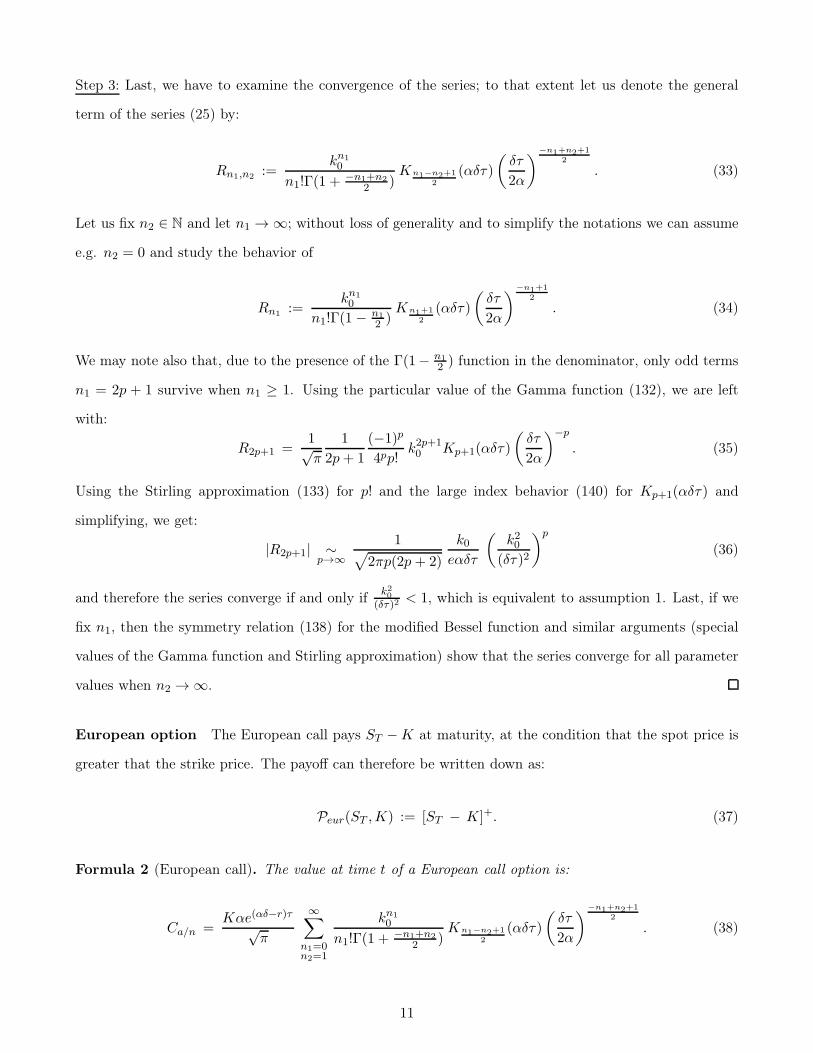
Formula 7 (European call). The value at time t of a European call option is:

Ceur =Kαe(γδ−r)τ√

π

∞∑

n1,n2=0n3=1

(−n1 + n3 + 1)n2 kn10 βn2

n1!n2!Γ(1 +−n1+n2+n3

2 )Kn1−n2−n3+1

2

(αδτ)

(

δτ

2α

)

−n1+n2+n3+12

. (92)

20

Proof. Like in the proof of formula 2, we remark that we can write:

Peur(Se(r−q+ω)τ+x,K) = K(ek+x − 1)1x>−k. (93)

Then, we use the Mellin-Barnes representation (see table 7 in appendix A):

ek+x − 1 =

c3+i∞∫

c3−i∞

(−1)−s3Γ(s3)(k + x)−s3ds32iπ

(−1 < c3 < 0) (94)

and we proceed exactly the same way than for proving Formula 6; the n3-summation in (92) starts in

n3 = 1 instead of n3 = 0, because the strip of convergence of (94) is reduced to < −1, 0 > instead of

< 0,∞ > in (85).

By difference of (83) and (92), we immediately obtain the formula for the cash-or-nothing call:

Formula 8 (Cash-or-nothing call). The value at time t of a cash-or-nothing call option is:

Cc/n =αe(γδ−r)τ√

π

∞∑

n1,n2=0

(−n1 + 1)n2 kn10 βn2

n1!n2!Γ(1 +−n1+n2

2 )Kn1−n2+1

2

(αδτ)

(

δτ

2α

)

−n1+n2+12

. (95)

5 Numerical tests

In this section, we start by determining what restriction is induced by assumption 1 in terms of accessible

option maturities, and we provide some precise estimates for the convergence speed and the truncation

errors of the series. Then, we compare the various pricing formulas established in the above with several

numerical tools, and demonstrate the reliability and efficiency of the results.

5.1 Accessible range of parameters

We start by remarking that the at-the-money (ATM) situation (St = K) is a favorable situation for

satisfying assumption 1. Indeed, in that case, we have:

|k0|δτ

=

∣

∣

∣

∣

r − q

δ+

√

α2 − (β + 1)2 −√

α2 − β2∣

∣

∣

∣

. (96)

In the symmetric model in particular, it is clear that

− 1 +r − q

δ<

r − q

δ+

√

α2 − 12 − α <r − q

δ(97)

21

and therefore assumption 1 is satisfied as soon as r − q < δ; according to the implied parameters in table

1, the smallest calibrated value for δ is 0.2483, therefore assumption 1 is satisfied (independently of α and

of other market parameters) as soon as the risk-free interest rate is smaller than 25%, which is of course

the case for most financial applications.

In the more general non at-the-money and non symmetric case, satisfying assumption 1 necessitates

some restriction on the option’s maturities, depending on the moneyness situation. Assuming that µ = 0

(as option prices are not sensitive to µ) and, introducing

ρ± :=log St

K

±δ − r + q − ω, (98)

then it is not hard to see that:

- If St > K (in-the-money (ITM) situation), then assumption 1 is satisfied if τ > ρ+ or τ < ρ−;

- If St < K (out-of-the-money (OTM) situation), then assumption 1 is satisfied if τ > ρ− or τ < ρ+.

In table 1, we illustrate this rule on several implied NIG parameters, calibrated in the literature on various

option markets: OBX options in Saebø (2009), S&P 500 options in Matsuda (2006); Albrecher & Schoutens

(2005) or Euro Stoxx 50 (SX5E) options in Schoutens & al. (2004).

Table 1: Maturities allowing that assumption 1 is satisfied, for some sets of implied NIG parameters.Other parameters: K = 4000, r = 1%, q = 0% and St = 3500 (OTM) or St = 4500 (ITM).

NIG parameters Accessible maturitiesα β δ OTM ITM

Saebø (2009) 8.9932 -4.5176 1.1528 τ > 0.077 τ > 0.208Matsuda (2006) 20.7408 -11.7308 0.2483 τ > 0.319 τ > 1.504Schoutens & al. (2004) 16.1975 -3.1804 1.0867 τ > 0.104 τ > 0.131Albrecher & Schoutens (2005) 18.4815 -4.8412 0.4685 τ > 0.226 τ > 0.341

5.2 Truncation error

In this subsection we estimate the rest of some series arising in our pricing formulas, in order to determine

what truncation has to be applied to obtain a desired level of precision in option prices. For simplicity

of notations, we perform the analysis in the symmetric model, but extension to the asymmetric case is

straightforward.

22

Cash-or-nothing Let us observe that the general term of the cash-or-nothing series (47) is the same

than the R2p+1 term introduced in (35) in the proof of formula 1:

R2p+1 :=1√π

1

2p+ 1

(−1)p

4pp!k2p+10 Kp+1(αδτ)

(

δτ

2α

)−p. (99)

Using the bound (36), we therefore know that, for ǫ > 0, there exists a rank pǫ such that the general term

of the series in the cash-or-nothing formula (47) is bounded by

|R2pǫ+1| ∼∣

∣

∣

∣

∣

1√

2πpǫ(2pǫ + 2)

k0eαδτ

(

k20(δτ)2

)pǫ∣

∣

∣

∣

∣

< ǫ. (100)

As a consequence of assumption 1, | k0eαδτ | < 1 and therefore, denoting by ⌈X⌉ the least integer greater or

equal to a real number X, it suffices to choose

pǫ =

⌈

log αǫ

2 log |k0δτ |

⌉

(101)

to be sure that all terms of order p ≥ pǫ are O(ǫ) in the series (47). Turning back to the n-variable (i.e.

n = 2p + 1), it follows from (101) that, definying

nǫ := 2pǫ + 1, (102)

then all terms of order n ≥ nǫ are O(ǫ) in the series of formula 3, and that the error in the option price

itself is bounded by

αe(αδ−r)τ√π

ǫ (103)

after the computation of nǫ + 1 terms.

Asset-or-nothing Recall the notations introduced in the proof of formula 1 for the general term of the

series:

Rn1,n2 :=kn10

n1!Γ(1 +−n1+n2

2 )Kn1−n2+1

2(αδτ)

(

δτ

2α

)

−n1+n2+12

(104)

and for the terms on the line n2 = 0:

Rn1 :=kn10

n1!Γ(1− n12 )

Kn1+12

(αδτ)

(

δτ

2α

)

−n1+12

. (105)

23

Let us fix n1 ∈ N and consider

∣

∣

∣

∣

Rn1,n2+1

Rn1,n2

∣

∣

∣

∣

=

∣

∣

∣

∣

∣

Γ(1 + −n1+n22 )

Γ(1 + −n1+n2+12 )

∣

∣

∣

∣

∣

∣

∣

∣

∣

∣

Kn1−n22

(αδτ)

Kn1−n2+12

(αδτ)

∣

∣

∣

∣

∣

√

δτ

2α. (106)

From the particular values of the Gamma functions (132), the ratio of Gamma functions in (106) is smaller

or equal to√π, and the ratio of Bessel functions is smaller than 1, as a consequence of the symmetry and

monotonicity relations (138) and (139). Hence,

∣

∣

∣

∣

Rn1,n2+1

Rn1,n2

∣

∣

∣

∣

<

√

πδτ

2α(107)

and, consequently, |Rn1,n2 | < |Rn1,0| = |Rn1 | for any n2 in N as soon as

τ <2α

πδ. (108)

Under this condition, all Rn1,n2 terms are therefore O(ǫ) as soon as n1, n2 ≥ nǫ where nǫ is the one

determined in (102), and, consequently, the error in the option price given formula 1 is bounded by

Kαe(αδ−r)τ√π

ǫ (109)

after the computation of (nǫ + 1)2 terms. Note that if (108) is not satisfied, the series still converges but

the maximum is not attained on the line n2 = 0, which complicates the estimation of the number of terms

to compute. We may nevertheless observe that (108) is a very reasonable condition: for instance, using

the implied parameters given in table 1 for SX5E options, we find τ < 9.49, which is very close to the

maximal expiry (10 years) quoted for options written on this underlying.

European Exactly the same analysis can be performed on the European option, resulting in an error

for the option price given by formula 2 bounded by

Kαe(αδ−r)τ√π

ǫ (110)

after the computation of nǫ(nǫ + 1) terms (because the n2 summation starts at n2 = 1). To illustrate

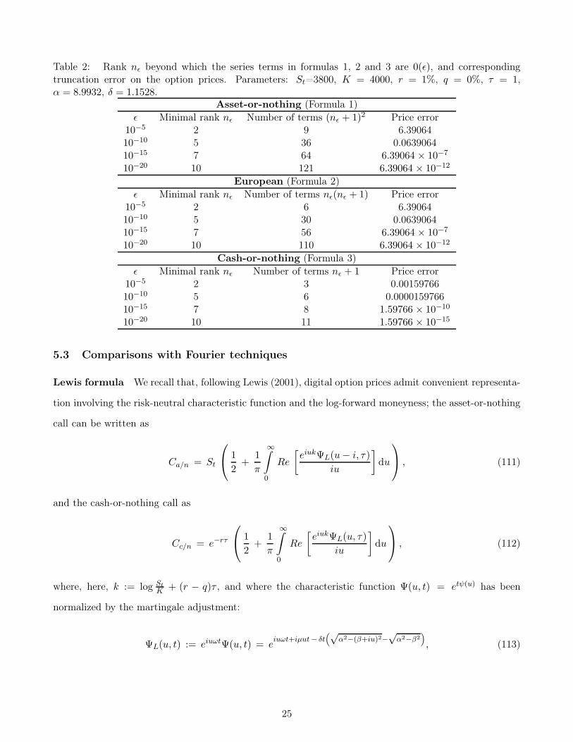
these observations, we summarize in table 2 the minimal rank, number of terms and price errors obtained

for the digital and European options for some realistic market parameters.

24

Table 2: Rank nǫ beyond which the series terms in formulas 1, 2 and 3 are 0(ǫ), and correspondingtruncation error on the option prices. Parameters: St=3800, K = 4000, r = 1%, q = 0%, τ = 1,α = 8.9932, δ = 1.1528.

Asset-or-nothing (Formula 1)

ǫ Minimal rank nǫ Number of terms (nǫ + 1)2 Price error10−5 2 9 6.3906410−10 5 36 0.063906410−15 7 64 6.39064 × 10−7

10−20 10 121 6.39064 × 10−12

European (Formula 2)

ǫ Minimal rank nǫ Number of terms nǫ(nǫ + 1) Price error10−5 2 6 6.3906410−10 5 30 0.063906410−15 7 56 6.39064 × 10−7

10−20 10 110 6.39064 × 10−12

Cash-or-nothing (Formula 3)

ǫ Minimal rank nǫ Number of terms nǫ + 1 Price error10−5 2 3 0.0015976610−10 5 6 0.000015976610−15 7 8 1.59766 × 10−10

10−20 10 11 1.59766 × 10−15

5.3 Comparisons with Fourier techniques

Lewis formula We recall that, following Lewis (2001), digital option prices admit convenient representa-

tion involving the risk-neutral characteristic function and the log-forward moneyness; the asset-or-nothing

call can be written as

Ca/n = St

1

2+

1

π

∞∫

0

Re

[

eiukΨL(u− i, τ)

iu

]

du

, (111)

and the cash-or-nothing call as

Cc/n = e−rτ

1

2+

1

π

∞∫

0

Re

[

eiukΨL(u, τ)

iu

]

du

, (112)

where, here, k := log St

K + (r − q)τ , and where the characteristic function Ψ(u, t) = etψ(u) has been

normalized by the martingale adjustment:

ΨL(u, t) := eiuωtΨ(u, t) = eiuωt+iµut− δt

(√α2−(β+iu)2−

√α2−β2

)

, (113)

25

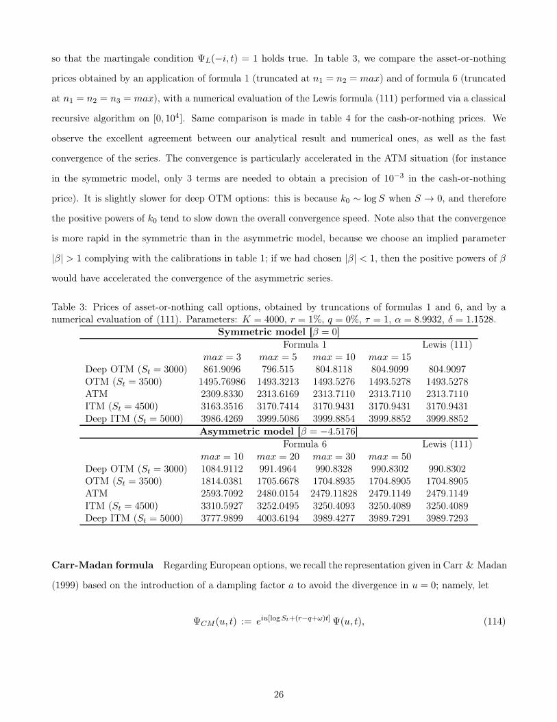
so that the martingale condition ΨL(−i, t) = 1 holds true. In table 3, we compare the asset-or-nothing

prices obtained by an application of formula 1 (truncated at n1 = n2 = max) and of formula 6 (truncated

at n1 = n2 = n3 = max), with a numerical evaluation of the Lewis formula (111) performed via a classical

recursive algorithm on [0, 104]. Same comparison is made in table 4 for the cash-or-nothing prices. We

observe the excellent agreement between our analytical result and numerical ones, as well as the fast

convergence of the series. The convergence is particularly accelerated in the ATM situation (for instance

in the symmetric model, only 3 terms are needed to obtain a precision of 10−3 in the cash-or-nothing

price). It is slightly slower for deep OTM options: this is because k0 ∼ log S when S → 0, and therefore

the positive powers of k0 tend to slow down the overall convergence speed. Note also that the convergence

is more rapid in the symmetric than in the asymmetric model, because we choose an implied parameter

|β| > 1 complying with the calibrations in table 1; if we had chosen |β| < 1, then the positive powers of β

would have accelerated the convergence of the asymmetric series.

Table 3: Prices of asset-or-nothing call options, obtained by truncations of formulas 1 and 6, and by anumerical evaluation of (111). Parameters: K = 4000, r = 1%, q = 0%, τ = 1, α = 8.9932, δ = 1.1528.

Symmetric model [β = 0]

Formula 1 Lewis (111)max = 3 max = 5 max = 10 max = 15

Deep OTM (St = 3000) 861.9096 796.515 804.8118 804.9099 804.9097OTM (St = 3500) 1495.76986 1493.3213 1493.5276 1493.5278 1493.5278ATM 2309.8330 2313.6169 2313.7110 2313.7110 2313.7110ITM (St = 4500) 3163.3516 3170.7414 3170.9431 3170.9431 3170.9431Deep ITM (St = 5000) 3986.4269 3999.5086 3999.8854 3999.8852 3999.8852

Asymmetric model [β = −4.5176]

Formula 6 Lewis (111)max = 10 max = 20 max = 30 max = 50

Deep OTM (St = 3000) 1084.9112 991.4964 990.8328 990.8302 990.8302OTM (St = 3500) 1814.0381 1705.6678 1704.8935 1704.8905 1704.8905ATM 2593.7092 2480.0154 2479.11828 2479.1149 2479.1149ITM (St = 4500) 3310.5927 3252.0495 3250.4093 3250.4089 3250.4089Deep ITM (St = 5000) 3777.9899 4003.6194 3989.4277 3989.7291 3989.7293

Carr-Madan formula Regarding European options, we recall the representation given in Carr & Madan

(1999) based on the introduction of a dampling factor a to avoid the divergence in u = 0; namely, let

ΨCM (u, t) := eiu[logSt+(r−q+ω)t] Ψ(u, t), (114)

26

Table 4: Prices of cash-or-nothing call options, obtained by truncations of formulas 3 and 8, and by anumerical evaluation of (111). Parameters: K = 4000, r = 1%, q = 0%, τ = 2, α = 8.9932, δ = 1.1528.

Symmetric model [β = 0]

Formula 3 Lewis (112)max = 3 max = 5 max = 10 max = 15

Deep OTM (St = 3000) 0.2127 0.2092 0.2095 0.2095 0.2095OTM (St = 3500) 0.3076 0.3073 0.3073 0.3073 0.3073ATM 0.4054 0.4054 0.4054 0.4054 0.4054ITM (St = 4500) 0.4973 0.4973 0.4973 0.4973 0.4973Deep ITM (St = 5000) 0.5793 0.5793 0.5793 0.5793 0.5793

Asymmetric model [β = −4.5176]

Formula 8 Lewis (112)max = 10 max = 20 max = 30 max = 50

Deep OTM (St = 3000) 0.2579 0.2360 0.2357 0.2357 0.2357OTM (St = 3500) 0.3523 0.3244 0.3240 0.3240 0.3240ATM 0.4544 0.4077 0.4074 0.4074 0.4074ITM (St = 4500) 0.5740 0.4823 0.4827 0.4827 0.4827Deep ITM (St = 5000) 0.7634 0.7277 0.5733 0.5452 0.5489

then the European call price admits the representation:

Ceur =e−a logK−rτ

π

∞∫

0

e−iu logKRe

[

ΨCM(u− (a+ 1)i, τ)

a2 + a− u2 + i(2a+ 1)u

]

du, (115)

where a < 0 < amax, and amax is determined by the square integrability condition ΨCM (−(a+1)i, τ) <∞.

In table 5 we compare the European prices obtained by formula 2 (truncated at n1 = n2 = max) and

formula 7 (truncated at n1 = n2 = n3 = max), with a numerical evaluation of the Carr-Madan formula

(115) on the interval [0, 104]. We also observe the excellent agreement between our analytical results and

the numerical ones, as well as the accelerated convergence for very short term options. For instance, when

τ = 1 day, (1+5)2 iterations are enough to obtain a precision of 10−3 in the option price in the symmetric

model; this is because, when St is close to K, then k0 ∼ (r − q + ω)τ and therefore when τ → 0 the

positive powers of k0 arising in formulas 2 and 7 accelerate the convergence of the series. Note that, on the

contrary, the short maturity case is not a favorable situation for a numerical evaluation of the Carr-Madan

formula, because of the presence of oscillations of the integrand that considerably slow down the numerical

Fourier inversion process.

27

Table 5: Prices of European call options of various maturities, obtained by truncations of formulas 2 and7, and by a numerical evaluation of (115). Parameters: St = K = 4000, r = 1%, q = 0%, α = 8.9932,δ = 1.1528.

Symmetric model [β = 0]

Formula 2 Carr-Madan (115)Maturity max = 3 max = 5 max = 10 max = 151 year 576.6432 580.4319 580.5260 580.5260 580.52601 month 150.8024 150.8651 150.8656 150.8656 150.86561 week 60.9649 60.9746 60.9747 60.9747 60.97471 day 15.4503 15.4515 15.4515 15.4515 15.4515

Asymmetric model [β = −4.5176]

Formula 7 Carr-Madan (115)Maturity max = 10 max = 20 max = 30 max = 501 year 790.330 679.6635 678.8152 678.8118 678.81181 month 173.6275 173.5547 173.5546 173.5546 173.55461 week 68.4327 68.4234 68.4234 68.4234 68.42341 day 16.7801 16.7790 16.7790 16.7790 16.7790

5.4 Comparisons with Monte Carlo simulations

Let n ∈ N\0 and define the family of independent and identically distributed random variables Z(i),

i = 1 . . . n, all distributed according to the symmetric NIG distribution Z(i) ∼ NIG(α, 0, δ, µ), and define

C(i)log := e−rτ

[

logStKe(r−q+ω)τ+Z

(i)

]+

= e−rτ [k0 + Z(i)]+ (116)

as well as

C(n)log :=

1

n

n∑

i=1

C(i)log. (117)

We know from the strong law of large numbers that C(n)log converges to the price of the log call option,

more precisely that

C(n)log −→ EQ

[

e−rτ[

logSTK

]+

|St]

(118)

almost surely when n→ ∞. Similarly, regarding power options, we define (in the European case):

C(i)pow := e−rτ

[

Saea((r−q+ω)τ+Z(i)) − K

]+, C(n)

pow :=1

n

n∑

i=1

C(i)pow (119)

and, for the capped digital option,

C(i)capped c/n := e−rτ 1−k0,−<Z(i)<−k0,+ , C

(n)capped c/n :=

1

n

n∑

i=1

C(i)capped c/n (120)

28

which converge to the European power call and to the capped cash-or-nothing call respectively. In table

6, we compare the results obtained via the Monte Carlo simulations (117), (119) and (120) for different

number of paths, with truncations of the pricing formulas 5, 4 and of (75). As expected, the results display

good agreement, but our series provide a far more precise price and a far more rapid convergence: for

instance, only 2 to 4 terms are needed to obtain a level of precision of 10−3 for the log call using formula

5, while the Monte Carlo price still features a relative error of 1% in the OTM case and even 4% in the

ITM case. Note also that, defining the 95% confidence interval by C(n)log ± 1.96σP /

√n where

σP :=

√

varC(i)logi=1...n, (121)

then its length vary between 0.0136 (OTM case) and 0.0187 (ITM case) after n = 1000 paths. Of

course the confidence interval could be reduced by increasing the number of paths (but then the Standard

Monte Carlo becomes time and resource consuming) or by introducing variance reduction techniques, such

as antithetic variates or importance sampling methods (see Su & Fu (2000) or the classical monograph

Glasserman (2004)). On the contrary, with our series expansions, the results are quasi instantaneous and

can easily be made as precise as one wishes, without introducing further sophistication.

Table 6: Prices of log, power and capped calls, obtained by Monte Carlo simulations (n paths) or truncationof formulas 5, 4 and series (75). Parameters: K− = K = 4000, K+ = 5000, r = 1%, q = 0%, τ = 2,α = 8.9932, δ = 1.1528, a = 1.2.

Log option (call)

Monte Carlo (117) Formula 5n = 100 n = 500 n = 1000 nmax = 1 nmax = 3 nmax = 5

OTM (St = 3500) 0.0826 0.1034 0.1002 0.1012 0.1008 0.1008ATM (St = 4000) 0.1537 0.1508 0.1509 0.1483 0.1482 0.1482ITM (St = 4500) 0.2428 0.2255 0.1923 0.2014 0.2014 0.2014

Power option (European)

Monte Carlo (119) Formula 4n = 100 n = 1000 n = 5000 max = 20 max = 40 max = 60

OTM (St = 3500) 12943.90 13976.71 14456.01 1429.53 14629.84 14629.84ATM (St = 4000) 17229.06 17263.31 17678.74 17843.79 17847.18 17847.18ITM (St = 4500) 20719.09 20310.75 21422.76 21126.01 21148.88 21148.89

Capped option (digital)

Monte Carlo (120) Series (75)n = 100 n = 1000 n = 5000 nmax = 1 nmax = 5 nmax = 10

OTM (St = 3500) 0.1764 0.1519 0.1262 0.1754 0.1355 0.1347ATM (St = 4000) 0.1862 0.1608 0.1598 0.1754 0.1575 0.1575ITM (St = 4500) 0.2058 0.1774 0.1672 0.1754 0.1702 0.1702

29

6 Concluding remarks

In this paper, we have proved two general formulas for pricing arbitrary path independent instruments

in the exponential NIG model, in the symmetric and asymmetric cases. These formulas allow to express

the Mellin transform of the instrument’s price as the product of the Mellin transform of the instrument’s

payoff and of the NIG probability density. Inverting the formulas by means of residue theory in C and

Cn has allowed us to derive practical closed-form pricing formulas for various path independent options

and contracts, under the form of quickly convergent series. The convergence of the series is guaranteed as

soon as a simple condition of the log forward moneyness and on the option’s maturity is fulfilled. We have

tested our results by comparing them with classical numerical methods, and provided precise estimate for

the convergence speed; notable feature is that a very reasonable number of terms is required to obtain an

excellent level of precision, and that the convergence is particularly fast for short term and at-the-money

options.

Future work should include, among others, an extension of the Mellin residue summation method to

path independent instruments on several assets, and to path dependent instruments. Asian options with

continuous geometric payoffs, in particular, should be investigated, because the characteristic function for

the geometric average is known exactly in the exponential NIG model (see Fusai & Meucci (2008)), for

both fixed and floating strikes.

Extension of the technique to Generalized Hyperbolic (GH) Lévy motions should also be considered.

GH distributions are not convolution-closed, that is, the Lévy processes they generate are not necessarily

distributed according to a GH distribution for increments of length t 6= 1 (exceptions being the NIG

process, which, as we know, is distributed according to a NIG distribution NIG(α, β, δt, µt) for all t, as

well as the generalized Laplace distribution). As a consequence, the Lévy symbol for the GH process

admits a more complicated representation than for the NIG process, and the martingale adjustment

must be estimated by a dichotomy method (see details in Prause (1999); Eberlein (2001)). However, the

probability density of the GH distribution has a very similar form to the NIG density (1), which allows

for the same convenient representation in terms of Mellin-Barnes integrals for the Bessel kernel, and for a

factorized pricing formula.

References

Abramowitz, M. and Stegun, I., Handbook of Mathematical Functions, Dover Publications, Mineola, NY(1972)

30

Aguilar, J. Ph., On expansions for the Black-Scholes prices and hedge parameters, Journal of MathematicalAnalysis and Applications 478(2), 973-989 (2019)

Aguilar, J. Ph. and Korbel, J., Simple Formulas for Pricing and Hedging European Options in the FiniteMoment Log-Stable Model, Risks 7, 36 (2019)

Aguilar, J. Ph., Some pricing tools for the Variance Gamma model, International Journal of Theoreticaland Applied Finance 23 (2020)

Albrecher, H. and Predota, M., On Asian option pricing for NIG Lévy processes, Journal of Computationaland Applied Mathematics 172, 153-168 (2004)

Albrecher, H. and Schoutens, W., Static hedging of Asian options under stochastic volatility models usingFast Fourier Transform. In: A. Kyprianou et al. (Eds), Exotic Options and Advanced Lévy models pp.129-148, John Wiley & Sons, Hoboken, NJ (2005)

Andrews, L.C., Special Functions of Mathematics for Engineers, McGraw-Hill Book Company, New York(1992)

Barndorff-Nielsen, O., Exponentially decreasing distributions for the logarithm of particle size, Proceedingsof the Royal Society of London 353, 401-419 (1977)

Barndorff-Nielsen, O., Normal inverse Gaussian distributions and the modeling of stock returns, Researchreport no 300, Department of Theoretical Statistics, Aarhus University (1995)

Barndorff-Nielsen, O., Normal inverse Gaussian distributions and stochastic volatility models, Scandina-vian Journal of Statistics 24(1), 1-133 (1997)

Bateman, H., Tables of Integral Transforms (vol. I and II), McGraw-Hill Book Company, New York (1954)

Bertoin, J., Lévy Processes, Cambridge University Press, Cambridge, New York, Melbourne (1996)

Black, F. and Scholes, M., The Pricing of Options and Corporate Liabilities, Journal of Political Economy81(3), 637-654 (1973)

Carr, P. and Madan, D., Option valuation using the Fast Fourier Transform, Journal of ComputationalFinance 2, 61-73 (1999)

Carr, P., Geman, H., Madan, D., Yor, M., The Fine Structure of Asset Returns: An Empirical Investiga-tion, Journal of Business 75(2), 305-332 (2002)

Carr, P. and Wu, L., The Finite Moment Log Stable Process and Option Pricing, The Journal of Finance58(2), 753-777 (2003)

Carr, P. and Wu, L., Time-changed Lévy processes and option pricing, Journal of Financial Economics71, 113-141 (2004)

Carr, P., Lee R. and Wu, L., Variance swaps on time-changed Lévy processes, Finance and Stochastics16, 335-355 (2012)

Cont, R. and Tankov, P., Financial Modelling with Jump Processes, Chapman & Hall, New York (2004)

Eberlein, E. and Keller,U., Hyperbolic distributions in finance, Bernoulli 1(3), 281-299 (1995)

Eberlein, E., Application of Generalized Hyperbolic Lévy Motions to Finance. In: Lévy Processes,Barndorff-Nielsen O.E., Resnick S.I., Mikosch T. (eds), Birkhauser, Boston, MA (2001)

31

Fang, F. and Oosterlee, C.W., A novel pricing method for European options based on Fourier cosine seriesexpansions, SIAM Journal on Scientific Computing 31, 826-848 (2008)

Figueroa-López, J.E., Lancette, S.R, , Lee, K. and Mi, Y., Estimation of NIG and VG models for highfrequency financial data. In: Handbook of Modeling High-Frequency Data in Finance, F. Viens, M.C.Mariani, I. Florescu (eds.), John Wiley & Sons, Hoboken, NJ (2012)

Flajolet, P., Gourdon, X. and Dumas, P., Mellin transforms and asymptotics: Harmonic sums, TheoreticalComputer Science 144, 3-58 (1995)

Fusai, G. and Meucci, A., Pricing discretely monitored Asian options under Lévy processes, Journal ofBanking & Finance 32(10), 2076–2088 (2008)

Giannone, D., Reichlin, L. and Small, D., Nowcasting: The real-time informational content of macroeco-nomic data, Journal of Monetary Economics 55(4), 665-676 (2008)

Glasserman, P., Monte Carlo methods in financial engineering, Springer Science & Business Media Vol.53,New York (2004)

Hanssen, A. and Øigård, T.A., The Normal inverse Gaussian distribution: a versatile model for heavy-tailed stochastic processes, Proceedings - ICASSP, IEEE International Conference on Acoustics, Speechand Signal Processing 6, 3986-3988 (2001)

Ivanov, R.V., Closed Form Pricing of European Options for a Family of Normal Inverse Gaussian Processes,Journal of Stochastic Models 29(4), 435-450 (2013)

Kirkby, J. L., Efficient Option Pricing by Frame Duality with the Fast Fourier Transform, SIAM Journalon Financial Mathematics 6(1), 713-747 (2015)

Lewis, A.L., A simple option formula for general jump-diffusion and other exponential Lévy processes,Available at SSRN 282110 (2001)

Luciano, E. and Semeraro, P., Multivariate time changes for Lévy asset models: Characterization andcalibration, Journal of Computational and Applied Mathematics 223(8), 1937-1953 (2010)

Madan, D., Carr, P. and Chang, E., The Variance Gamma Process and Option Pricing, European FinanceReview 2, 79-105 (1998)

Mandelbrot, B., The Variation of Certain Speculative Prices, The Journal of Business 36(4), 384-419(1963)

Matsuda, K., Calibration of Lévy Option Pricing Models: Applications to S& P 500 Futures option, PhDThesis City University of New York (2006)

Mittnik, S. and Rachev, S., Stable Paretian models in finance, John Wiley & Sons, Hoboken, NJ (2000)

Neuberger, A., The log contract, Journal of Portfolio Management 20, 74-80 (1994)

Papantoleon, A., An introduction to Lévy Processes with applications in finance, arXiv:0804.0482 (2008)

Prause, K, The generalized hyperbolic model: estimation, financial derivatives and risk measures, PhDthesis, Institut für Mathematische Statistik, Albert-Ludwigs-Universität Freiburg (1999)

Rachev, S., Kim, Y., Bianchi, M., Fabozzi, F., Financial models with Lévy processes and volatility clus-tering, John Wiley & Sons, Hoboken, NJ (2011)

32

Ribeiro, C. and Webber, N., A Monte Carlo Method for the Normal Inverse Gaussian Option ValuationModel using an Inverse Gaussian Bridge, City University preprint (2003)

Rydberg, T., The Normal inverse Gaussian Lévy process: simulation and approximation, Communicationsin Statistics. Stochastic Models 13, 887-910 (1997)

Saebø, K., Pricing Exotic Options with the Normal Inverse Gaussian Market Model using Numerical PathIntegration, Master’s Thesis Norwegian University of Science and Technology (2009)

Schoutens, W., Lévy processes in finance: pricing financial derivatives, John Wiley & Sons, Hoboken, NJ(2003)

Schoutens, W., Simons, E., and Tistaert, J., A perfect calibration! Now what?, Wilmott magazine 2004(2)(2004)

Su, Y., and Fu., M.C., Importance sampling in derivative securities pricing, 2000 Winter SimulationConference Proceedings Vol. 1. (2000)

Taleb, N.N., The Black Swan: The Impact of the Highly Improbable, Random House Publishing Group,New York (2010)

Tankov, P., Pricing and Hedging in Exponential Lévy Models: Review of Recent Results. In: Paris-Princeton Lectures on Mathematical Finance. Lecture Notes in Mathematics, vol 2003, Springer, Berlin,Heidelberg (2010)

Venter, J. and de Jongh, P., Risk estimation using the Normal inverse Gaussian distribution, The Journalof Risks 2, 1-25 (2002)

Wilmott, P., Paul Wilmott on Quantitative Finance, Wiley & Sons, Hoboken, NJ, 2006

Zeng, P. and Kwok, Y.K., Pricing barrier and Bermudan style options under time-changed Lévy processes:fast Hilbert transform approach, SIAM Journal on Scientific Computing 36(3), B450-B485 (2014)

A Brief review of the Mellin transform

We present an overview of the one-dimensional Mellin transform; this theory is explained in full detail in

Flajolet et al. (1995), and table of Mellin transforms can be found in any monograph on integral transforms

(see e.g. Bateman (1954)).

1. The Mellin transform of a locally continuous function f defined on R+ is the function f∗ defined by

f∗(s) :=

∞∫

0

f(x)xs−1 dx. (122)

The region of convergence α < Re(s) < β into which the integral (122) converges is often called the

fundamental strip of the transform, and sometimes denoted < α, β >.

33

2. The Mellin transform of the exponential function is, by definition, the Euler Gamma function:

Γ(s) =

∞∫

0

e−x xs−1 dx (123)

with strip of convergence Re(s) > 0. Outside of this strip, it can be analytically continued, except at

every negative s = −n integer where it admits the singular behavior

Γ(s) ∼s→−n

(−1)n

n!

1

s+ n, n ∈ N. (124)

In table 7 we summarize the main Mellin transforms used in this paper, as well as their convergence strips.

Table 7: Mellin pairs used throughout the paper.f(x) f∗(s) Convergence strip

e−ax a−sΓ(s) < 0,∞ >e−ax − 1 a−sΓ(s) < −1, 0 >Kν(ax) a−s2s−2Γ

(

s−ν2

)

Γ(

s+ν2

)

< |Re(ν)|,∞ >Kν(a

√x2+b2)

(x2+b2)ν2

as2 2

s2−1b

s2−νΓ( s2)Kν− s

2(ab) < 0,∞ >

3. The inversion of the Mellin transform is performed via an integral along any vertical line in the strip

of convergence:

f(x) =

c+i∞∫

c−i∞

f∗(s)x−sds

2iπc ∈ (α, β) (125)

and notably for the exponential function one gets the so-called Cahen-Mellin integral :

e−x =

c+i∞∫

c−i∞

Γ(s)x−sds

2iπ, c > 0. (126)

4. When f∗(s) is a ratio of products of Gamma functions of linear arguments:

f∗(s) =Γ(a1s+ b1) . . .Γ(ams+ bm)

Γ(c1s+ d1) . . .Γ(cls+ dl)(127)

then one speaks of a Mellin-Barnes integral, whose characteristic quantity is defined to be

∆ =m∑

k=1

ak −l

∑

j=1

cj . (128)

34

∆ governs the behavior of f∗(s) when |s| → ∞ and thus the possibility of computing (125) by summing

the residues of the analytic continuation of f∗(s) right or left of the convergence strip:

∆ < 0 f(x) = −∑

Re(s)>β

Res[

f∗(s)x−s]

,

∆ > 0 f(x) =∑

Re(s)<α

Res[

f∗(s)x−s]

.

(129)

For instance, in the case of the Cahen-Mellin integral one has ∆ = 1 and therefore:

e−x =∑

Re(s)<0

Res[

Γ(s)x−s]

=

∞∑

n=0

(−1)n

n!xn (130)

as expected from the usual Taylor series of the exponential function.

B Some useful special functions identities

We list some properties of special functions that are used throughout the paper; more details can be found

e.g. in Abramowitz & Stegun (1972); Andrews (1992).

B.1 Gamma function

Particular values The Gamma function Γ(s) has been defined in (123) for Re(s) > 0; integrating by

parts shows that it satisfies the functional relation Γ(s+ 1) = sΓ(s); as Γ(1) = 1, it follows that

Γ(n+ 1) = n! , n ∈ N (131)

and that the analytic continuation of Γ(s) to the negative half-plane is singular at every negative integer

−n with residue (−1)n

n! . Other useful identities include Γ(12) =√π and, more generally,

Γ

(

1

2− n

)

=(−1)n4nn!

(2n)!

√π

Γ

(

1

2+ n

)

=(2n)!

4nn!

√π.

(132)

for n ∈ N.

35

Stirling approximation We recall the well-known Stirling approximation for the factorial:

n! ∼n→∞

√2πnnn e−n. (133)

Legendre duplication formula For any s ∈ C, we have:

Γ(

s2

)

Γ(s)=

√π

2s−1

1

Γ(

s+12

) . (134)

Pochhammer symbol The Pochhamer symbol (a)n, sometimes denoted by the Appel symbol (a, n),

and also called rising factorial, is defined by

(a)n :=Γ(a+ n)

Γ(a), a /∈ Z−. (135)

The definition (135) extends continuously to negative integers thans to the functional relation Γ(s+ 1) =

sΓ(s), thanks to the relation:

(−k)n =

(−1)nk!

(k − n)!0 ≤ n < k

0 n > k.

(136)

where k ∈ N.

B.2 Bessel functions

The modified Bessel function of the second kind, also called MacDonald function, can be defined by the

Mellin integral

Kν(z) :=1

2

(z

2

)ν∞∫

0

e−t−z2

4t t−ν−1 dt (137)

for |argz| < π4 . It follows that Kν(z) has the symmetry property:

Kν(z) = K−ν(z) (138)

and has monotonous absolute values:

0 ≤ ν1 < ν2 =⇒ |Kν1(z)| < |Kν2(z)|. (139)

36

Large index When ν → ∞, one has the following behavior:

Kν(z) ∼ν→∞

√

π

2ν

( ez

2ν

)−ν. (140)

Large argument (Hankel’s expansion) Define the following sequence:

a0(ν) = 1

ak(ν) =(4ν2 − 12)(4ν2 − 32) . . . (4ν2 − (2k − 1)2)

k!8k, k ≥ 1.

(141)

Then, for large z and fixed ν, we have:

Kν(z) =z→∞

√

π

2ze−z

∞∑

k=0

ak(ν)

zk. (142)

In particular, when 4ν2 − 1 = 0, i.e. when ν = 12 , all the ak(ν) are null in definition (141) when k ≥ 1,

and we are left with:

K 12(z) =

√

π

2ze−z (143)

for all z.

37