15
Improved Tilt Sensing in an LGS-based Tomographic AO System Based on Instantaneous PSF Estimation Jean-Pierre Véran AO4ELT3, 27-31 May 2013
| Date post: | 15-Mar-2016 |
| Category: |
Documents |
| Upload: | caesar-kline |
| View: | 30 times |
| Download: | 6 times |

Improved Tilt Sensing in an LGS-based Tomographic AO System Based on
Instantaneous PSF Estimation
Jean-Pierre VéranAO4ELT3, 27-31 May 2013

AO fields (NFIRAOS)
• 17”x17” science field
• 70” diameter LGS asterism
• 120” diameter “technical” field
• To pick-off NGS sources
• Used to sense tip, tilt and tilt anisoplanatism (NGS modes)
• All LGS-based MCAO, LTAO MOAO systems have a similar arrangement

NGS modes in a tomographic LGS system
• NGS modes = tip, tilt and tilt anisoplanatism• How well we can correct the NGS modes sets the sky coverage• For NFIRAOS, 3 NGSs (2 T/T and 1 2x2 Shack-Hartmann)• Problem: NGSs are usually far away from the science field and
are therefore poorly corrected (even if MCAO is implemented)• Spot centroiding error
– Decreases with sharper core– Decreases with higher number of photons in the core
• Spot centroiding error propagates to reduce NGS mode correction

Mitigation #1Improved control
• A more sophisticated control strategy allows increasing the exposure time (so more photons in the core) without being severely penalized by the increase in servo-lag error
• Increased sky coverage with optimal correction of tilt and tilt-anisoplanatism modes in laser-guide-star multiconjugate adaptive optics, Correia, Carlos; Véran, Jean-Pierre; Herriot, Glen; Ellerbroek, Brent; Wang, Lianqi; Gilles, Luc, JOSA A, vol. 30, issue 4, p. 604, 2013– Uses LQG control of all the NGS modes– Improves the sky coverage by ~20% on NFIRAOS, compared
to simple type-I control

Mitigation #2Image sharpening
• Use a DM in each of the NGS WFS paths to sharpen the NGS spots
• The DM is driven based on a wave-front estimate in the direction of the NGS, derived from the current 3D estimate of the turbulence obtained from the LGSs
• Pros:– Potential for spectacular improvements in sky coverage
• Cons:– DM is driven in open-loop– Significant increase in cost and in complexity (opto-mechanics
+ software)

NGS sharpening on NFIRAOS
Lianqi Wang, TMT

Spot centroiding using long exposure reference
• NFIRAOS baseline: unconstrained matched filters, based on Gaussian fit to long exposure spot image.
• Example: H-band, WFE=600nm RMS (SR=0.4%), PDE=600, rn=3e-, TT=0mas RMS, 100 uncorrelated spot images, 8x8 pixels, 5.5mas/pixel (Nyquist)
X-filter Y-filter
Average spot image Gaussian fit
Examples of instantaneous spot images
Corresponding instantaneous PSFs
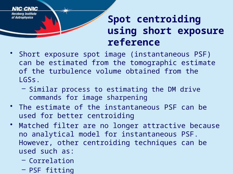
Spot centroiding using short exposure reference
• Short exposure spot image (instantaneous PSF) can be estimated from the tomographic estimate of the turbulence volume obtained from the LGSs.– Similar process to estimating the DM drive commands for
image sharpening• The estimate of the instantaneous PSF can be used for better
centroiding• Matched filter are no longer attractive because no analytical
model for instantaneous PSF. However, other centroiding techniques can be used such as: – Correlation– PSF fitting
Inspiration
• Deconvolution from wave-front sensing (DWFS)– Deconvolution from wave-front sensing: a new technique for
compensating turbulence-degraded images, J. Primot, G. Rousset, and J. C. Fontanella, JOSA A, Vol. 7, Issue 9, pp. 1598-1608 (1990)
– Use WFS measurements to aid speckle imaging– Improves performance of traditional speckle imaging
techniques– Early days of AO

PSF fitting
• Find (a,b,c) that minimize:Where:I(x,y) is the recorded spot image, PSF(x,y) is the estimated
instantaneous PSF, and σx,y is the noise at each pixel.• Carry out the minimization in the Fourier domain, using the
Levenberg-Marquardt algorithm for quick convergence• Trivial case of finding the photometry and astrometry of a stellar
field image knowing the PSF (only one star here!)
€
I(x,y) − c *PSF(x − a,y −b)σ x,y
∑2

SimulationStep 1: Creation
• Create 100 random phase screens with spatial frequency distribution f^[-2,-3]
• For each screen– Remove P/T/T and renormalize to RMS=[100,300,600]– Create instantaneous PSF – Scale total to [100,200,300,400,500,600] PDE (store S1)– Apply tilt=N(0,[0,0.1,0.2,0.3,0.4,0.5])pix– Apply [8x8,4x4] window (store S2)– Apply photon + readout noise (3e-) (store S3)
• Compute:– Long exposure PSF (from S3)– Unconstrained matched filters (from LEPSF + 3e- noise)
SimulationStep 2: Processing
• For each image:– Apply matched filter– Correlate with long exposure PSF and find maximum of
correlation function– Correlate with instantaneous PSF and find maximum of
correlation function– Apply PSF fitting using long exposure PSF– Apply PSF fitting using instantaneous PSF
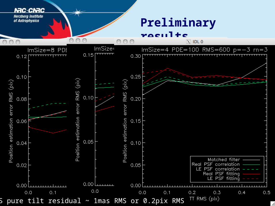
Preliminary results
NFIRAOS pure tilt residual ~ 1mas RMS or 0.2pix RMS
Conclusion
• Improved centroiding using an estimate of the instantaneous PSF might be an interesting alternative to image sharpening– Implementation only requires a bit of additional software
• Work in progress• Preliminary results are encouraging• PSF fitting could probably be improved by not trying to estimate
the amplitude of the PSF from each image– Use amplitude of long exposure PSF instead
• Errors in estimating the instantaneous PSF needs to be addressed


