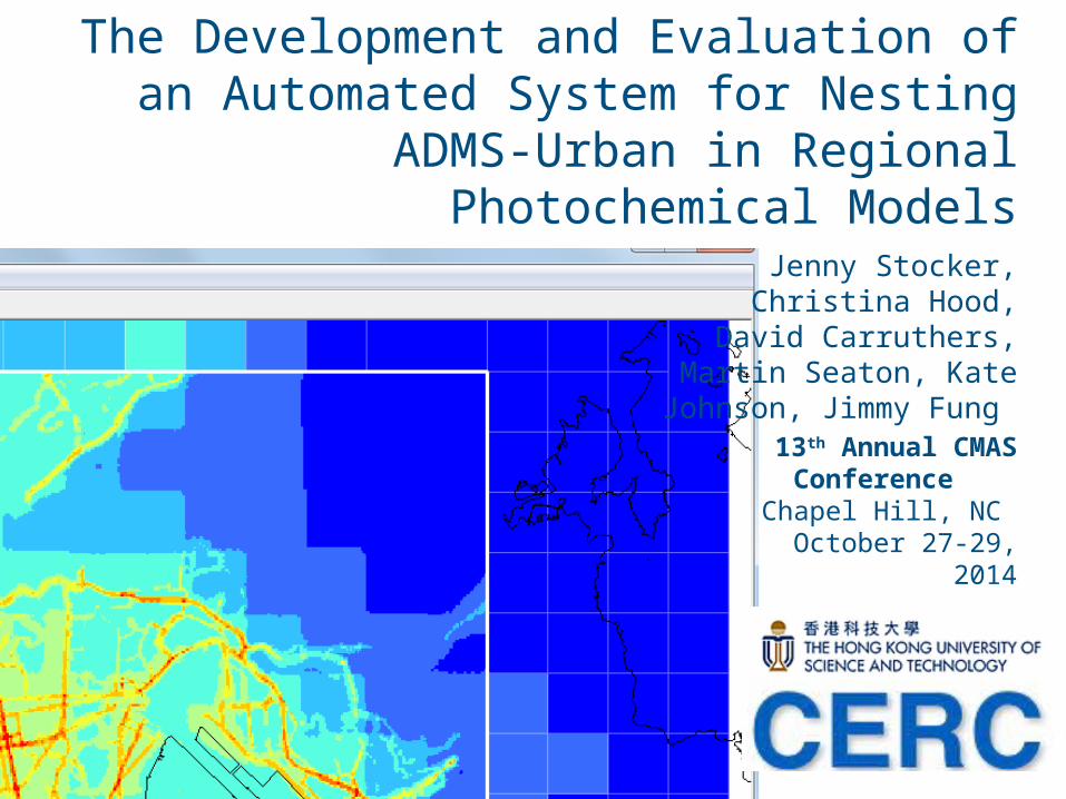
Jenny Stocker, Christina Hood, David Carruthers, Martin Seaton, Kate Johnson, Jimmy Fung The Development and Evaluation of an Automated System for Nesting ADMS-Urban in Regional Photochemical Models 13 th Annual CMAS Conference Chapel Hill, NC October 27-29, 2014
Transcript
Jenny Stocker, Christina Hood, David Carruthers,
Martin Seaton, Kate Johnson, Jimmy Fung
The Development and Evaluation of an Automated System for Nesting ADMS-Urban
in Regional Photochemical Models
13th Annual CMAS Conference
Chapel Hill, NC October 27-29, 2014
13th Annual CMAS Conference, Chapel Hill, NC, October 27-29, 2014
Contents
• Introduction• Nesting concept• System implementation• Example use of system:
– Input data– System configuration– Run times– Validation methodology– Results
• Conclusions
13th Annual CMAS Conference, Chapel Hill, NC, October 27-29, 2014
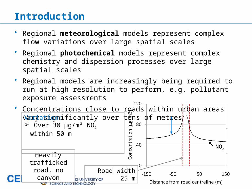
• Regional meteorological models represent complex flow variations over large spatial scales
• Regional photochemical models represent complex chemistry and dispersion processes over large spatial scales
• Regional models are increasingly being required to run at high resolution to perform, e.g. pollutant exposure assessments
• Concentrations close to roads within urban areas vary significantly over tens of metres
Introduction
Road width 25 m
Heavily trafficked road, no canyon
Variation: Over 30 µg/m³ NO2 within 50 m
NO2
13th Annual CMAS Conference, Chapel Hill, NC, October 27-29, 2014
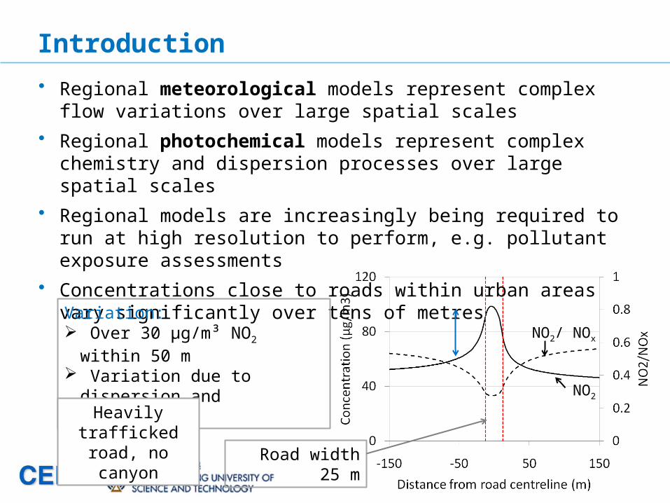
• Regional meteorological models represent complex flow variations over large spatial scales
• Regional photochemical models represent complex chemistry and dispersion processes over large spatial scales
• Regional models are increasingly being required to run at high resolution to perform, e.g. pollutant exposure assessments
• Concentrations close to roads within urban areas vary significantly over tens of metres
Introduction
Road width 25 m
Variation: Over 30 µg/m³ NO2 within 50 m Variation due to dispersion and
chemistry
Heavily trafficked road, no canyon
NO2
NO2/ NOx
13th Annual CMAS Conference, Chapel Hill, NC, October 27-29, 2014
• Regional meteorological models represent complex flow variations over large spatial scales
• Regional photochemical models represent complex chemistry and dispersion processes over large spatial scales
• Regional models are increasingly being required to run at high resolution to perform, e.g. pollutant exposure assessments
• Concentrations close to roads within urban areas vary significantly over tens of metres
• Issues with running regional models at high resolution include:– Difficult to include explicit modelling of roads and near-source features, e.g.
street canyons– Run times and data storage requirements become prohibitive– Some parameterisations within the model become invalid, in particular
cloud parameterisations in WRF
Introduction
13th Annual CMAS Conference, Chapel Hill, NC, October 27-29, 2014
• What are the advantages of a nested system of models?
Introduction
Model feature Model
Regional (eg grid based) Local (eg Gaussian plume)
Domain extent Country (few 1000 km) City (50km)
Meteorology Spatially and temporally varying from meso-scale models
Usually spatially homogeneous
Dispersion in low wind speed conditions
Models stagnated flows correctly
Limited modelling of stagnated flows
Deposition and chemical processes
Reactions over large spatial and temporal scales
Simplified reactions over short-time scales
Source resolution Low High
Validity Background receptors Background, roadside and kerbside receptors
13th Annual CMAS Conference, Chapel Hill, NC, October 27-29, 2014
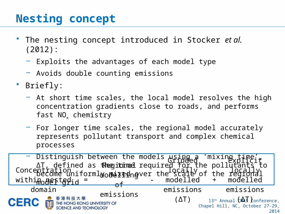
• The nesting concept introduced in Stocker et al. (2012):– Exploits the advantages of each model type
– Avoids double counting emissions
• Briefly:– At short time scales, the local model resolves the high concentration
gradients close to roads, and performs fast NOx chemistry
– For longer time scales, the regional model accurately represents pollutant transport and complex chemical processes
– Distinguish between the models using a ‘mixing time’, ΔT, defined as the time required for the pollutants to become uniformly mixed over the scale of the regional model grid
Nesting concept
Concentration within nested domain
=Regional
modelling of emissions
-Gridded locally
modelled emissions (ΔT)
+Explicit locally
modelled emissions (ΔT)
13th Annual CMAS Conference, Chapel Hill, NC, October 27-29, 2014
Nesting concept
Concentration within nested domain
=Regional
modelling of emissions
-Gridded locally
modelled emissions (ΔT)
+Explicit locally
modelled emissions (ΔT)
Regional model calculations
performed off-line i.e. nesting is a post-processing system
Consistent emissions used in both models
Regional meteorology drives local model
Theoretically, ΔT depends on grid scale and meteorology; in practice, ΔT fixed at 1 to 2 hours
Nesting calculations performed separately for each regional model grid cell
13th Annual CMAS Conference, Chapel Hill, NC, October 27-29, 2014
System implementationMeso-scale
meteorological data (WRF)
Emissions data
Regional model concentration
output
KeyUtilityData
Model run
13th Annual CMAS Conference, Chapel Hill, NC, October 27-29, 2014
System implementationMeso-scale
meteorological data (WRF)
Emissions data
Meteorological data for use in
local model
Regional model concentration
output
KeyUtilityData
Model run
13th Annual CMAS Conference, Chapel Hill, NC, October 27-29, 2014
System implementationMeso-scale
meteorological data (WRF)
Emissions data
Meteorological data for use in
local model
Regional model concentration
output
Local upwind background
Local modelGridded run for
background (0.5 hr)
Nesting background
KeyUtilityData
Model run
13th Annual CMAS Conference, Chapel Hill, NC, October 27-29, 2014
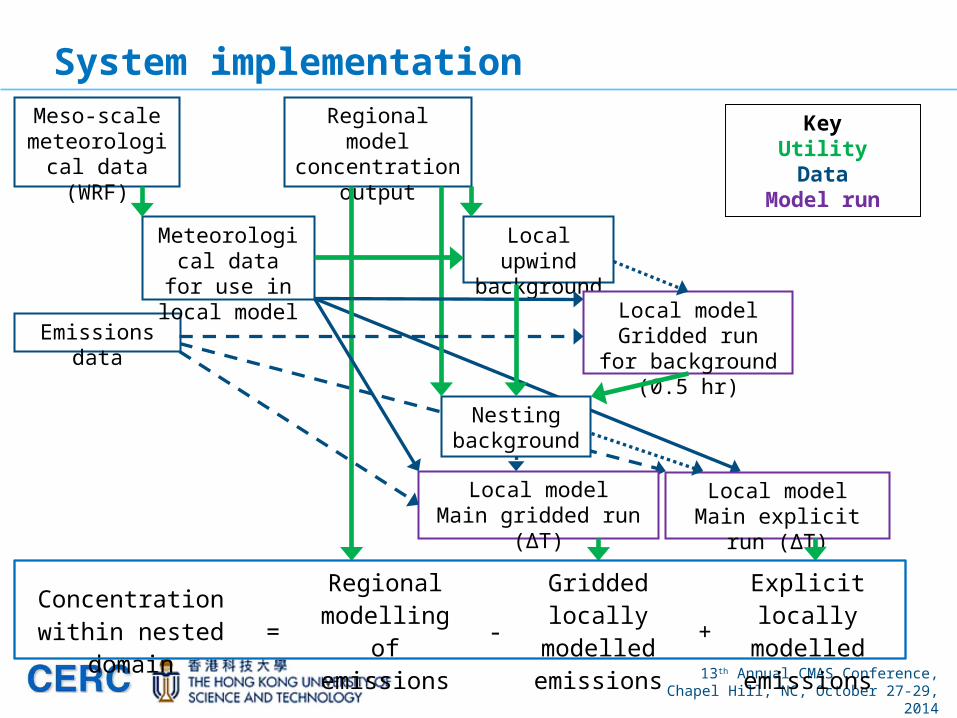
System implementationMeso-scale
meteorological data (WRF)
Emissions data
Meteorological data for use in
local model
Regional model concentration
output
Local upwind background
Local modelGridded run for
background (0.5 hr)
Local modelMain gridded run (ΔT)
Local modelMain explicit run (ΔT)
Nesting background
KeyUtilityData
Model run
13th Annual CMAS Conference, Chapel Hill, NC, October 27-29, 2014
Concentration within nested domain
=Regional
modelling of emissions
-Gridded locally
modelled emissions
+Explicit locally
modelled emissions
System implementationMeso-scale
meteorological data (WRF)
Emissions data
Meteorological data for use in
local model
Regional model concentration
output
Local upwind background
Local modelGridded run for
background (0.5 hr)
Local modelMain gridded run (ΔT)
Local modelMain explicit run (ΔT)
Nesting background
KeyUtilityData
Model run
13th Annual CMAS Conference, Chapel Hill, NC, October 27-29, 2014
System implementation: components
Regional model data: WRF, CAMx, CMAQ, EMEP4UK
Local model: ADMS-Urban
13th Annual CMAS Conference, Chapel Hill, NC, October 27-29, 2014
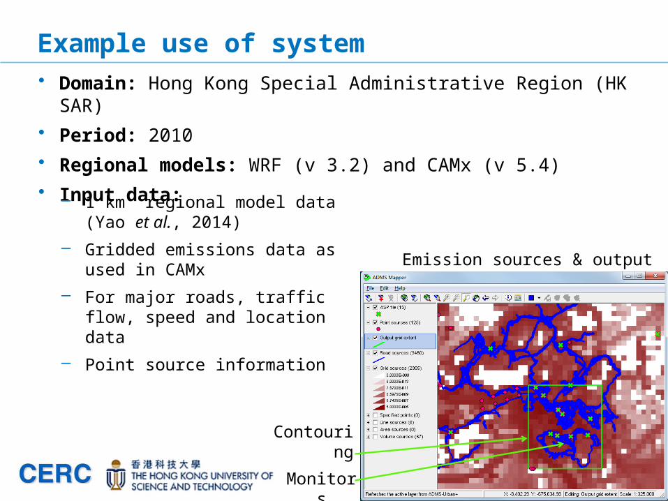
• Domain: Hong Kong Special Administrative Region (HK SAR)
• Period: 2010
• Regional models: WRF (v 3.2) and CAMx (v 5.4)
• Input data:
Example use of system
Emission sources & output locations
Contouring domain
Monitors
– 1 km regional model data (Yao et al., 2014)
– Gridded emissions data as used in CAMx
– For major roads, traffic flow, speed and location data
– Point source information
13th Annual CMAS Conference, Chapel Hill, NC, October 27-29, 2014
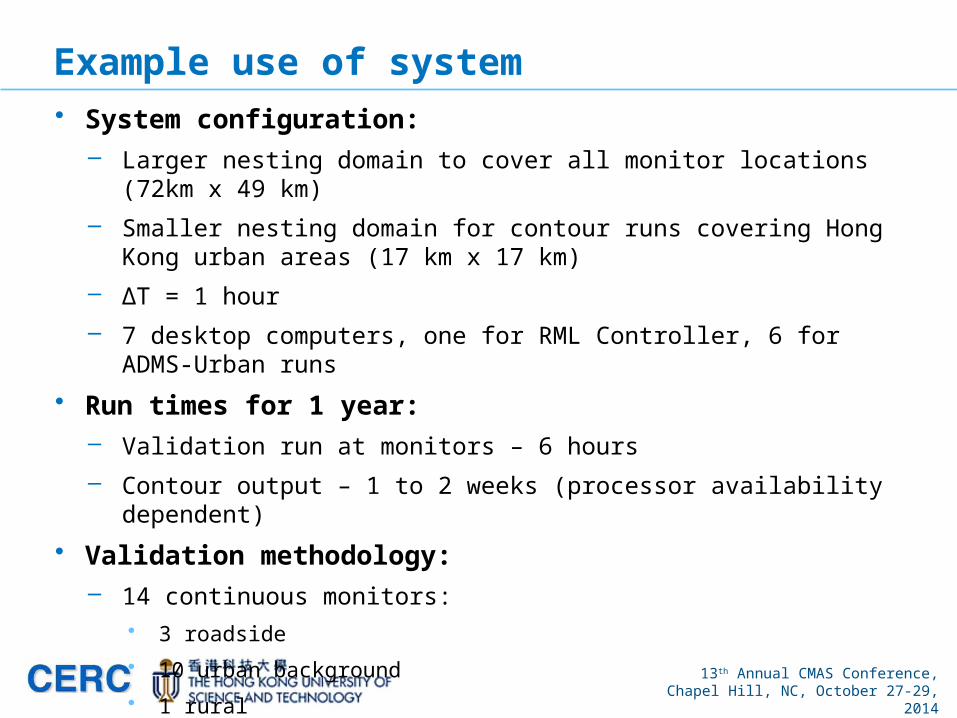
• System configuration: – Larger nesting domain to cover all monitor locations (72km x 49 km)
– Smaller nesting domain for contour runs covering Hong Kong urban areas (17 km x 17 km)
– ΔT = 1 hour
– 7 desktop computers, one for RML Controller, 6 for ADMS-Urban runs
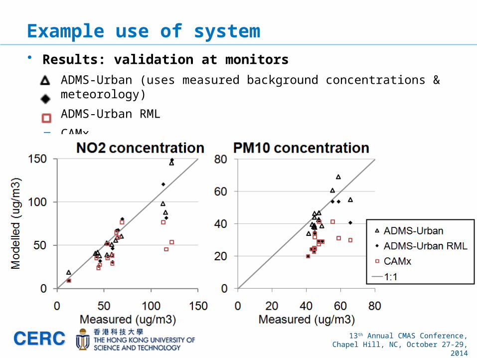
• Run times for 1 year:– Validation run at monitors – 6 hours
13th Annual CMAS Conference, Chapel Hill, NC, October 27-29, 2014
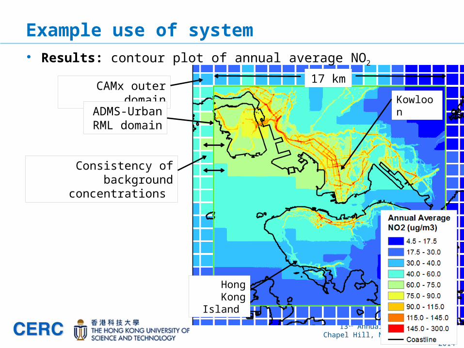
• Results: contour plot of annual average NO2
Example use of system
CAMx outer domain
ADMS-Urban RML domain
17 km
Consistency of background concentrations
Hong Kong Island
Kowloon
13th Annual CMAS Conference, Chapel Hill, NC, October 27-29, 2014
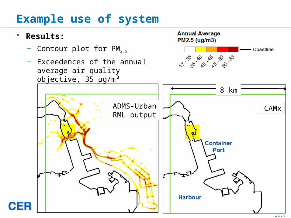
• Results:
– Contour plot for PM2.5
– Exceedences of the annual average air quality objective, 35 µg/m³
Example use of system
8 km
ADMS-Urban RML output
CAMx
13th Annual CMAS Conference, Chapel Hill, NC, October 27-29, 2014
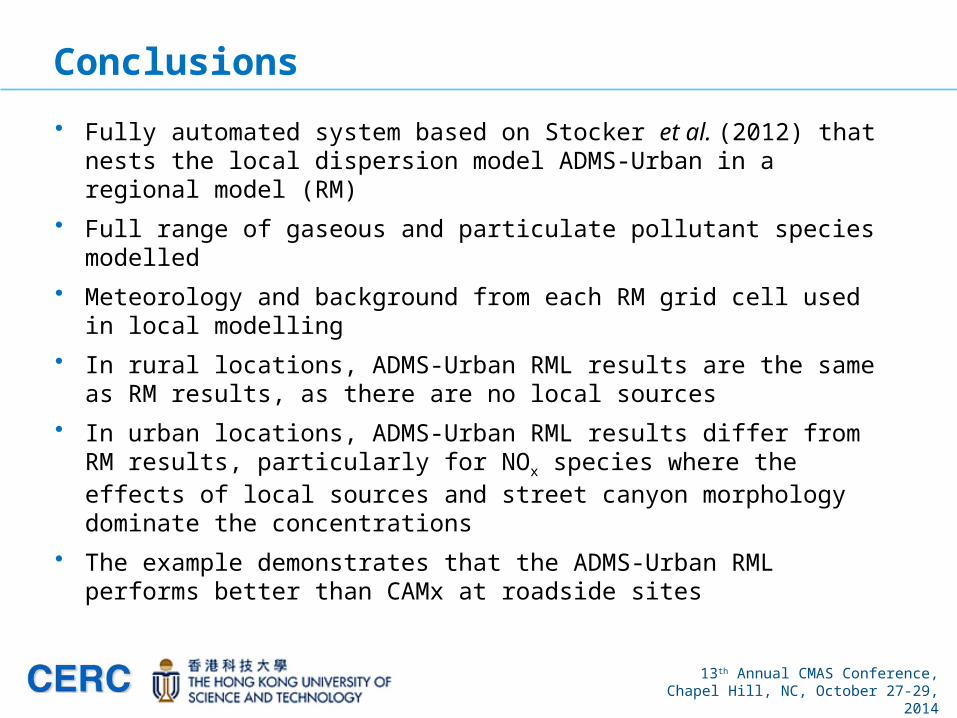
Conclusions
• Fully automated system based on Stocker et al. (2012) that nests the local dispersion model ADMS-Urban in a regional model (RM)
• Full range of gaseous and particulate pollutant species modelled
• Meteorology and background from each RM grid cell used in local modelling
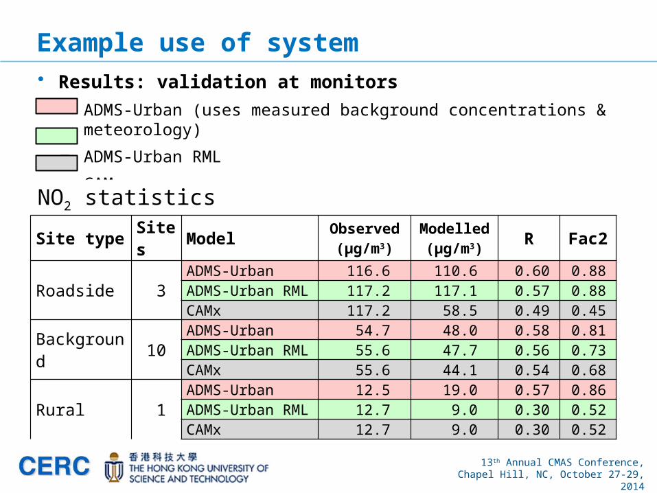
• In rural locations, ADMS-Urban RML results are the same as RM results, as there are no local sources
• In urban locations, ADMS-Urban RML results differ from RM results, particularly for NOx species where the effects of local sources and street canyon morphology dominate the concentrations
• The example demonstrates that the ADMS-Urban RML performs better than CAMx at roadside sites
13th Annual CMAS Conference, Chapel Hill, NC, October 27-29, 2014
Acknowledgements
The ADMS-Urban RML system has been developed in collaboration with researchers from the Hong Kong University of Science and Technology, supported by the Hong Kong Environmental Protection Department.
13th Annual CMAS Conference, Chapel Hill, NC, October 27-29, 2014
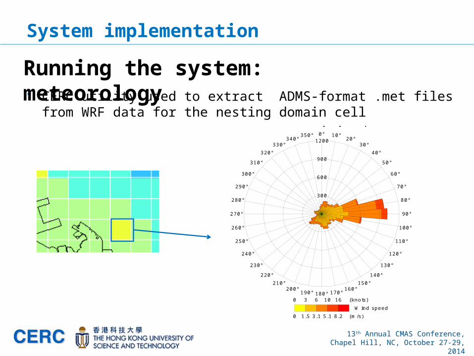
• CERC utility used to extract ADMS-format .met files from WRF data for the nesting domain cell
System implementation
Running the system: meteorology
WRF data for Causeway Bay example domain
0
0
3
1.5
6
3.1
10
5.1
16
8.2
(knots)
(m/s)W ind speed
0° 10°20°
30°40°
50°
60°
70°
80°
90°
100°
110°
120°
130°
140°150°
160°170°180°190°
200°210°
220°
230°
240°
250°
260°
270°
280°
290°
300°
310°
320°330°
340°350°
300
600
900
1200
13th Annual CMAS Conference, Chapel Hill, NC, October 27-29, 2014
• Results: contour plot of annual average O3
Example use of system
CAMx outer domain
ADMS-Urban RML domain
15 km
Consistency of background concentrations
Hong Kong Island
Kowloon
13th Annual CMAS Conference, Chapel Hill, NC, October 27-29, 2014
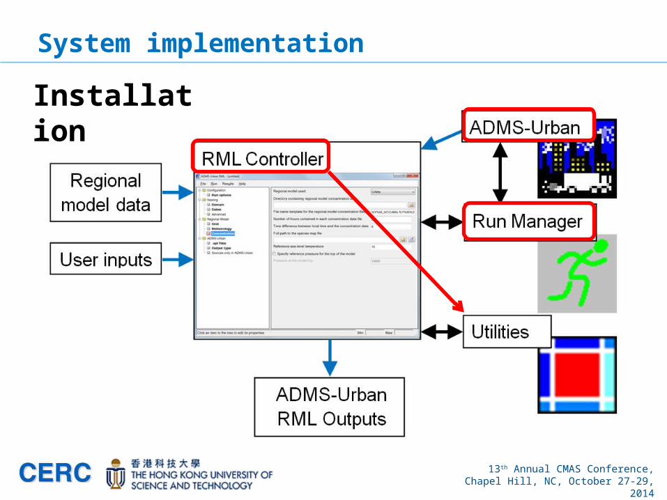
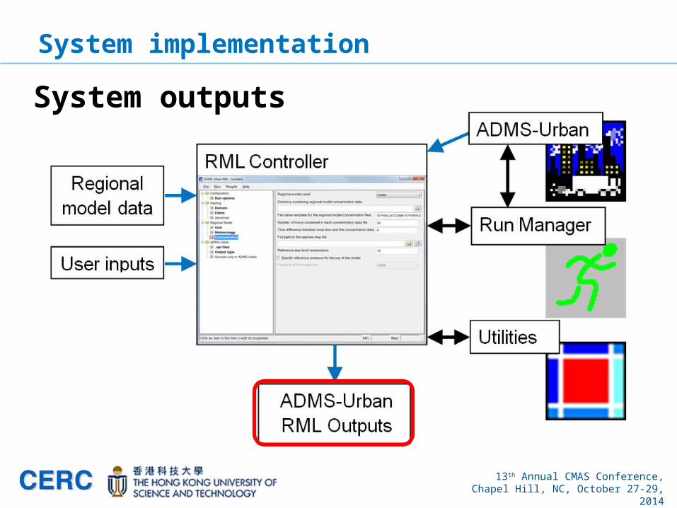
System implementation
Installation
13th Annual CMAS Conference, Chapel Hill, NC, October 27-29, 2014
System implementation
System inputs
13th Annual CMAS Conference, Chapel Hill, NC, October 27-29, 2014
System implementation
Running the system
13th Annual CMAS Conference, Chapel Hill, NC, October 27-29, 2014


![[Peter Carruthers] Introducing Persons](https://static.documents.pub/doc/80x56/577cb2841a28aba7118c0da6/peter-carruthers-introducing-persons.jpg)

