A REVIEW OF THE EQUATIONS OF MECHANICS

MEEN 673: NONLINEAR FINITE ELEMENT ANALYSIS

Read: Chapter 2

CONTENTS

Continuum assumption Kinematics of deformation Kinetics: Stress vector Cauchy’s formula Balance of linear momentum Balance of angular momentum Conservation of Energy

JN Reddy - 1 Lecture Notes on NONLINEAR FEM

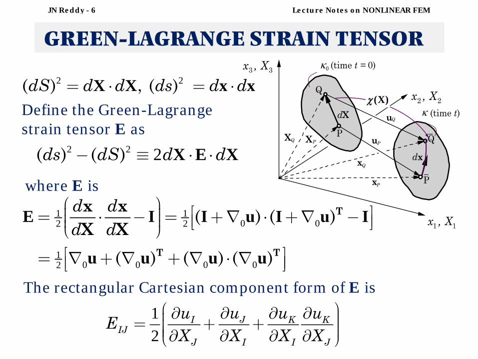
V 0

m( , t) limV

xρ∆ →

∆≡

∆Continuum assumption

The study of motion and deformation of a continuum can be broadly classified into four basic categories:

(1)Kinematics (strain-displacement equations)(2) Kinetics (balance of linear and angular momentum)(3) Thermodynamics (first and second laws of

thermodynamics)(4) Constitutive equations (stress-strain relations)

In the study of deformation and motion of solid bodies, we make the simplifying assumption for convenience that the matter is distributed continuously, without any macroscopic gaps or empty spaces; that is, we disregard the molecular structure of matter.

JN Reddy - 2 Lecture Notes on NONLINEAR FEM

E2ˆ

3 3x , X

2 2x , X

1 1x , X

κO

•

0κ

( ),tX

Reference configuration,

X

X Xx

u Current configuration, κ

Particle X occupying position X

Particle X occupying position x

0Rκ κ

E eˆ ˆ,1 1

E e3 3ˆ ˆ,

KINEMATICS OF SOLIDS

(x1, x2, x3) are the spatial (current) coordinates.

Material Description:

(X1, X2, X3) are the material coordinates.

0( , ), ( , )t x χ X X χ X

( , ) ( , )t t u X x X XDisplacement vector:

JN Reddy - 3 Lecture Notes on NONLINEAR FEM

AN EXAMPLE

Consider the uniform deformation of a square block ofside 2 units and initially centered at \bf X=(0,0). If the deformation is defined by the mapping

(a) sketch the deformation, and (c) compute the displacements.

1 2 1 2 2 3 33 5 0 5 4 e e eˆ ˆ ˆ( ) . .( ) ( )X X X Xχ X

Problem statement:

Solution:(a) From the given mapping, we have in matrix form, we have

1 1 2 2 2 3 33 5 0 5 4. . , ,x X X x X x X

JN Reddy - 4 Lecture Notes on NONLINEAR FEM

AN EXAMPLE (continued)

(−1,−1) (1,−1)

(−1,1) (1,1)

X1 , x1

X2 , x2

(2,3)

(3,5)

(4,3)

(5,5)(3.5,4)

( )Xχ

1 1ˆ ˆ,E e

2 2ˆ ˆ,E e

F E2ˆ( )

1 1ˆ ˆ( )F E e

1 ˆ( )F A

• •

• •

• •

•

•

• •

2.0 3.0 4.0 5.0(0,0)

2.0

3.0

4.0

5.0

°

°

°

°

2ˆ ˆ=A e

1 2 1 2

1 1 2 31 1 4 31 1 5 5

1 1 3 5

( , ) ( , )( , ) ( , )( , ) ( , )( , ) ( , )( , ) ( , )

X X x x

1 1 2

2 2 3 3

1 1 2

2 2 3 3

3 5 0 54

1 5 0 54

x . X . X ,x X , x X .X . x . x ,X x , X x .

(a)

(b) 2 2 313 5 0 5 4 0 ˆ ˆ ˆ. . Xu x X e e e

Mapping

JN Reddy - 5 Lecture Notes on NONLINEAR FEM

GREEN-LAGRANGE STRAIN TENSOR

XQ

Q

P Q_

XP

xP P_

xQ

uQ

uP

0κ

dx

dX κ

(time t = 0)

(time t)

1 1x , X

2 2x , X

3 3x , X

(X)χ

2 2 ( ) , ( )dS d d ds d dX X x x

2 2 2( ) ( )ds dS d d X E X

Define the Green-Lagrange strain tensor E as

1 10 02 2

10 0 0 02

T

T T

x xX X

( ) ( )

( ) ( ) ( )

d dd d

E I I u I u I

u u u u

where E is

12

JI K KIJ

J I I J

uu u uEX X X X

The rectangular Cartesian component form of E is

JN Reddy - 6 Lecture Notes on NONLINEAR FEM

2 2 2

31 1 211

1 1 1 1

2 2 2

32 1 222

2 2 2 2

2

3 133

3 3

12

12

12

,uu u uEX X X X

uu u uEX X X X

u u uEX X

2 2

32

3 3

3 31 2 1 1 2 212

2 1 1 2 1 2 1 2

3 3 31 1 1 2 213

3 1 1 3 1 3 1 3

223

3

12

12

12

uX X

u uu u u u u uEX X X X X X X X

u u uu u u u uEX X X X X X X X

uEX

3 3 31 1 2 2

2 2 3 2 3 2 3

u u uu u u uX X X X X X X

The rectangular Cartesian components in explicit form are given by

GREEN-LAGRANGE STRAIN TENSOR

1X

2X

3X

E1ˆ

E2ˆ

E3ˆ

11E

X1−face

X3−faceX2−face

21E

31E22E

32E

12E

33E

23E13E

th thStrain in the direction onthe faceIJE I J

Deformed body

JN Reddy - 7 Lecture Notes on NONLINEAR FEM

INFITESIMAL STRAIN TENSOR

If E is of the order in , then we mean

If terms of the order can be omitted, then

can be approximated as

O( ) 0 u

0O( ) asI

J

uX

2O( )12

JI K KIJ

J I I J

uu u uEX X X X

2

0 0

1 02

12

TE

O( ) as

( )

JIIJ

J I

uuEX X

ε u u

, the infinitesimal strain tensor

JN Reddy - 8 Lecture Notes on NONLINEAR FEM

KINETICS: Stress Vector

or Cauchy’s Lemma

Plane 1

∆f

∆aF1

F2

nF3 F4

−∆Fn−

0ˆ lim

aa

(-n) ftlim ∆a 0

ˆ

a

(n) ft

ˆ ˆ(n) (-n)t t ˆ ˆ(-n) (n)t t

JN Reddy - 9 Lecture Notes on NONLINEAR FEM

Kinetics - 10

Traction Vector: Examples

z

y

x

F

F

F

nNormal component

Shear componentˆ n i

F

F F i FF i0 cosA A θ 0A

JN Reddy - 10 Lecture Notes on NONLINEAR FEM

Kinetics - 11

n

z

y

x

−F

t(i)

t( )

θ

−F

n

Traction Vector: Examples

nF t ˆ( )A

0 0iF t ˆ( )A

0 cosA A θ

JN Reddy - 11 Lecture Notes on NONLINEAR FEM

CAUCHY STRESS TENSOR-1

1x

2x3x •A

• B

nt ˆ

n

x1

x3

x2

− t3

− t2

− t1

1e 2e3e

s∆2s∆

1s∆

3s∆

n

nt ˆ

3ˆ−e

2ˆ−e

1ˆ−e

ˆ ˆ( ) ( )ˆ ˆ ˆ ˆ ˆσ and σ ; , σn nt n t e t e e ej j i ij j i ji j ij i jt nσ σ σ = ⋅ = = = = Kinetics - 14

1 1 2 2 3 3 s s s s v vt t t t f aρ ρ∆ ∆ ∆ ∆ ∆ ∆

1 1 2 2 3 3

1 1 2 2 3 3

30

e n e n e n

e n e n e n e n n

ˆ ˆ ˆ ˆ ˆ ˆ( ) ( ) ( ) ( )

As , we obtainˆ ˆ ˆ ˆ ˆ ˆ ˆ ˆ ˆ( ) ( ) ( ) j j

h

h

t t t t a f

t t t t t

plane direction

JN Reddy - 12 Lecture Notes on NONLINEAR FEM

CAUCHY’S FORMULA

1x

2x3x •A

• B

nt ˆ

n

x1

x3

x2

− t3

− t2

− t1

1e 2e3e

s∆2s∆

1s∆

3s∆

n

nt ˆ

3ˆ−e

2ˆ−e

1ˆ−e

ˆ ˆ( ) ( )ˆ ˆ ˆσ and σ ,n nt n e t t ei i i j ji i ij jt n σ σ = ⋅ = = = Kinetics - 14

1 1 2 2 3 3 s s s s v vt t t t f aρ ρ∆ ∆ ∆ ∆ ∆ ∆

1 1 2 2 3 3

1 1 2 2 3 3

30

n e n e n e

n e n e n e n e n

ˆ ˆ ˆ ˆ ˆ ˆ( ) ( ) ( ) ( )

As , we obtainˆ ˆ ˆ ˆ ˆ ˆ ˆ ˆ ˆ( ) ( ) ( ) ( )i i

h

h

t t t t a f

t t t t t

Kinetics - 14plane direction

JN Reddy - 13 Lecture Notes on NONLINEAR FEM

Kinetics - 14

AN EXAMPLEProblem: Given the following stress tensor components in Cartesian coordinates

5 2 02 1 00 0 3

[ ] MPa

(a) Show the stress components on the stress cube.(b) Determine the traction vectors(c) Sketch the traction vectors on the stress cube.

)ˆ()ˆ()ˆ( and,, kji ttt

Solution: We have

xz

y

Stress cube3 MPa

5 MPa2 MPa

1 MPa2 MPa(a)

ktjitjit

k

j

i

ˆ3

ˆˆ2

ˆ2ˆ5

)ˆ(

)ˆ(

)ˆ(

−=

−−=

−=(b)

j i

k

JN Reddy - 14 Lecture Notes on NONLINEAR FEM

Kinetics - 15

5 2 0 5 2 02 1 0 2 1 00 0 3 0 0 3

[ ] MPa ,x x

y y

z z

t nt nt n

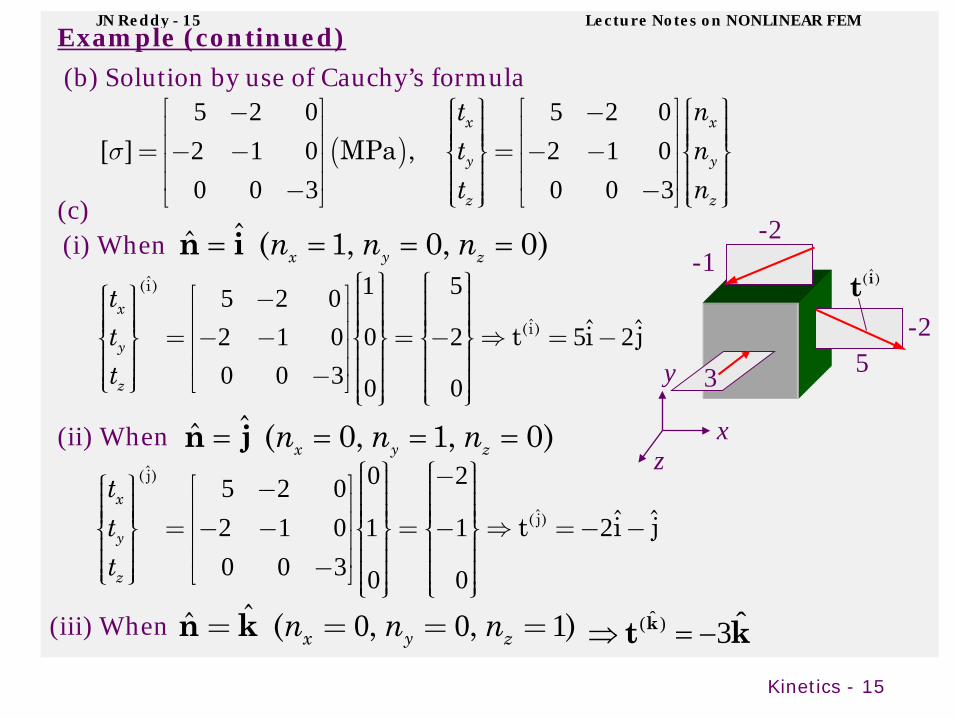
(b) Solution by use of Cauchy’s formula

(i) When )0,0,1(ˆˆ ==== zyx nnnin1 55 2 0

2 1 0 0 2 5 20 0 3 0 0

ˆ(i )

ˆ(i ) ˆ ˆt i jx

y

z

ttt

(ii) When )0,1,0(ˆˆ ==== zyx nnnjn0 25 2 0

2 1 0 1 1 20 0 3 0 0

ˆ( j)

ˆ( j) ˆ ˆt i jx

y

z

ttt

(iii) When 0 0 1n kˆ ( , , )x y zn n n kt k ˆ3)ˆ( −=⇒

xz

y 5-2

)ˆ(it

-2-1

3

(c)

Example (continued)JN Reddy - 15 Lecture Notes on NONLINEAR FEM

Kinetics - 16

With reference to a rectangular Cartesian system , the components of the stress dyadic at a certain point of a continuous medium are given by

Determine stress vector and its normal and tangential components at the point on the plane

which is planning through the point.

1 2 3( , , )x x x

200 400 300400 0 0300 0 100

[ ] psi.

1 2 3 1 2 32 2( , , ) constantx x x x x x

Problem statement:

AN EXAMPLEJN Reddy - 16 Lecture Notes on NONLINEAR FEM

Kinetics - 17

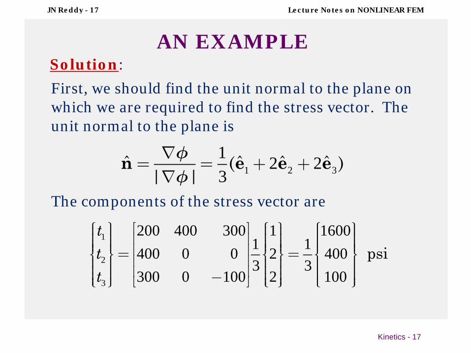
AN EXAMPLESolution: First, we should find the unit normal to the plane on which we are required to find the stress vector. The unit normal to the plane is

The components of the stress vector are

1 2 31 2 23

n e e eˆ ˆ ˆ ˆ( )| |

1

2

3

200 400 300 1 16001 1400 0 0 2 4003 3

300 0 100 2 100 psi

ttt

JN Reddy - 17 Lecture Notes on NONLINEAR FEM

Kinetics - 18

Solution (continued):

The traction vector normal to the plane is given by

and the traction vector projected onto the plane (i.e., shear traction) is given by

The magnitudes are

1 2 3

26009

2600 2 227

n n n n

e e e

ˆ ˆ ˆ ˆ( ( ) )

ˆ ˆ ˆ( ) psi

nn

t t

1 2 3100 118 16 4327

n e e e ˆ ˆ ˆ ˆ( ) ( ) psi.ns nn t t t

2600 288 89 468 919

. psi, . psi.nn nn ns nst t t t

)ˆ(nt

nP

nt nnn ˆtt es ns stnt nˆ( ) ˆnnt

•

JN Reddy - 18 Lecture Notes on NONLINEAR FEM

Mass-Momenta - 19

Balance of Linear Momentumin the Lagrangian Description

The time rate of change of total linear momentum of a given continuum equals the vector sum of all external forces acting on the continuum. This also known as Newton’s Second Law.

Newton's First Law. Newton's First Law states that an object will remain at rest or in uniform motion in a straight line unless acted upon by an external force.

0 0 0

0 0 0

0

0 0

0 0

0 0 0

ρ ρ

ρ ρ

ρ ρ

t f v

vn f

vf

ˆ

d d dt

d d dt

dt

t d

0 f d

d

d

0

JN Reddy - 19 Lecture Notes on NONLINEAR FEM

Mass-Momenta - 20

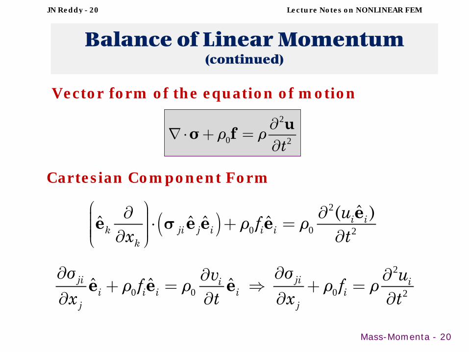
Balance of Linear Momentum(continued)

Vector form of the equation of motion2

0 2

uσ fρ ρt

2

0 0 2

2

0 0 0 2

ee e e e

e e e

ˆ( )ˆ ˆ ˆ ˆ

ˆ ˆ ˆ

i ik ji j i i i

k

ji jii ii i i i i

j j

uρ f ρx t

σ σv uρ f ρ ρ f ρx t x t

Cartesian Component Form

JN Reddy - 20 Lecture Notes on NONLINEAR FEM

Mass-Momenta - 21

Balance of Linear Momentum(continued)

2

0 0 2

23111 21 1

0 1 0 21 2 3

23212 22 2

0 2 0 21 2 3

213 23 33 3

0 3 0 21 2 3

ji ii

j

σ uρ f ρx t

σσ σ uρ f ρx x x t

σσ σ uρ f ρx x x t

σ σ σ uρ f ρx x x t

Cartesian Component Form (expanded form)

JN Reddy - 21 Lecture Notes on NONLINEAR FEM

Balance of Angular Momentum

The principle of balance of angular momentum can bestated as: the time rate of change of the total moment ofmomentum for a continuum is equal to vector sum of the moments of external forces acting on the continuum. We assume that there are no body (volume dependent) couples M:

0lim /V

V∆ →

∆ ∆ =M 0

Dd d dDt

Γ Ω Ω

× Γ + × Ω = × Ω∫ ∫ ∫x t x f x v

Then the balance of angular momentum requires

which results in the symmetry of the Cauchy stress tensor:T or ij ji = =σ σ

JN Reddy - 22 Lecture Notes on NONLINEAR FEM

Balance of Energy(in spatial description)

The first law of thermodynamics can be stated as: the time rate of the total energy is equal to the sum of the rate of work done by the external forces and the change of heat content per unit mass. The second law of thermodynamics provides a restriction on the inter-convertibility of energies (e.g., thermal to mechanical). The first law can be expressed as ( is the internal energy density, is the internal heat generation, and d is the symmetric part of the velocity gradient)

( ) ( )12

1 :2c

d De d d g ddt Dt

Ω Ω Ω

⋅ + Ω = ⋅ Ω + − ∇ ⋅ + Ω∫ ∫ ∫v v v v σ d q

which results in :cde gdt

= − ∇ ⋅ +σ d q

ce g

JN Reddy - 23 Lecture Notes on NONLINEAR FEM

Beam Theories 24

SUMMARYIn these lectures we have covered the following topics with some examples:

JN Reddy

Continuum assumption Kinematics of deformation:

Introduced the Green-Lagrangestrain tensor

Kinetics: Defined Cauchy stressvector

Cauchy’s formula is derived andCauchy stress tensor is introduced

Balance of linear and angular momenta Conservation of energy (the first law)

JN Reddy - 24 Lecture Notes on NONLINEAR FEM