26
MONTANA STATE UNIVERSITY Gravitational Wave Astronomy An Introduction to Emission Sources and Data Analysis John Pribyl 5/2/2014
| Date post: | 09-May-2017 |
| Category: |
Documents |
| Upload: | johnnypribyl |
| View: | 216 times |
| Download: | 1 times |

MONTANA STATE UNIVERSITY
Gravitational Wave Astronomy
An Introduction to Emission Sources and Data Analysis
John Pribyl
5/2/2014

1
Table of Contents
1 Introduction 2 2 Sources of Gravitational Wave Emission
2.1 High Frequency. . . . . . . . . . . . . . . . . . . . . 5
2.1.1 Ligo Overview. . . . . . . . . . . . . . . . . . . 5 2.1.2 Compact Binaries. . . . . . . . . . . . . . . . . 7 2.1.3 Stellar Core Collapse. . . . . . . . . . . . . . . 8 2.1.4 Periodic Emitters. . . . . . . . . . . . . . . . . 8 2.1.5 Stochastic Background. . . . . . . . . . . . . . 9 2.2 Low Frequency. . . . . . . . . . . . . . . . . . . . . . 10
2.2.1 LISA Overview. . . . . . . . . . . . . . . . . . . 10 2.2.2 Coalescing Binary Black Holes. . . . . . . . . . 12 2.2.3 Periodic Emitters. . . . . . . . . . . . . . . . . 12 2.2.4 Stochastic Background. . . . . . . . . . . . . . 13 2.3 Very Low Frequency and Ultra Low Frequency. . . . 13
2.3.1 VLF Pulsars. . . . . . . . . . . . . . . . . . . . . 13
2.3.2 ULF B-Mode Polarization. . . . . . . . . . . . . 14
3 Data Analysis
3.1 Detection Probability. . . . . . . . . . . . . . . . . . 15
3.1.1 Significance and Confidence. . . . . . . . . . . 15 3.1.2 Χ2 Likelihood and Goodness of Fit Test. . . . 15 3.1.3 Neyman-Pearson Approach. . . . . . . . . . . 16 3.2 Filtering. . . . . . . . . . . . . . . . . . . . . . . . . . 17
3.2.1 Constant Frequency Fourier Transform. . . . 17 3.2.2 Matched Filtering in 0-Mean Gaussian Noise 18 3.2.3 Templates. . . . . . . . . . . . . . . . . . . . . 19 3.2.4 Nyquist Theorem and Aliasing. . . . . . . . . 20 3.2.5 Maximum Likelihood Estimator. . . . . . . . 20 3.2.6 Bayesian Inference. . . . . . . . . . . . . . . . 21 3.2.7 MCMC Methods. . . . . . . . . . . . . . . . . 22
4 Summary 24 5 Acknowledgements 25

2
1 Introduction
Gravitational waves (GW) are incredibly small rippling oscillations
predicted by Einstein’s theory of General Relativity (GR) that transit the
fabric of space-time. They are the most energetic events in the known
universe, and are emitted by events as cataclysmic as the collision of two
black holes. However, these energetic ripples have proven to be
exceedingly elusive. Although GWs are prohibitively small (~10-21 or
smaller), a direct detection will likely occur in the next 5 years. By nature,
their interaction with matter is immensely feeble. The impact of this is that
GWs will eventually provide generous unobserved insights that pierce
deeply into the nature of their sources and out to the far reaches of the
universe. After analyzing the data and recovering all of the enclosed
information, GWs will measure the propagation speed (and consequently
the mass of) the graviton, provide the most stringent test of GR to date,
provide the equation of state of neutron stars, and provide insight into
countless other astrophysical phenomena. Additionally, there is a very
strong potential to discover new, inconceivable marvels that have hitherto
been buried somewhere in the recesses of the universe.
The tidal and quadrupolar elements of GWs cause them to stretch an
object in one direction while squeezing it in another. To envision this,
consider a piece of elastic. Now, grab the elastic with two hands before
pulling the hands apart horizontally. This will cause the elastic to stretch
horizontally while it compensates by squeezing together vertically in a
manner that roughly illustrates the field produced by GWs. The resulting
field may, in principle, be observed using Pulsar Timing Arrays (PTA) or
ground and space-based Laser Interferometers (LI).
Conservation of mass and linear momentum respectively prohibit the
monopole or dipole moments from radiating. Thus, the quadrupole
moment provides the lowest order source of GW emission. The
quadrupole formula [1] depends upon the density and may be
approximated by
∫ (1)

3
Where, omitting the prefactor, the amplitude of the gravitational wave
strain depends upon 1/r and not upon 1/r3
(2)
A further approximation using the virial theorem [2] provides the upper
bound for a non-spherical emission (spherical bodies will have no
quadrupole moment and as such will not radiate GWs)
(3)
This upper bound provides the highest possible strain amplitude that
ought to be examined. GWs are still undetectable as a result of their
prohibitive size. However, Joseph Taylor and Russel Hulse successfully
discovered the first binary pulsar system in 1974 [3]. They observed the
system over the two decades that followed before indirectly confirming the
emission of GWs. In 1993, they succeeded in showing that the period of
the binary was decreasing at precisely the rate that Einstein’s quadrupole
formula had predicted some 70 years earlier.
GR requires these waves to propagate in either a plus (+) or a cross (×)
polarization state. However, several alternative theories of gravity have
presented four additional polarization states. If GR were modified slightly,
it would be theoretically possible to observe GWs in two helicity-0 modes
(Transverse breathing mode, and Longitudinal mode) and two helicity-1
shear modes in addition to the + and × states. [4] The basis tensors for
these six states are:
(4)
Where the first two are those predicted by GR. In this way (among others),
a direct observation of GWs and subsequent characterization of the waves

4
will enable a test of the current theory of gravity under extreme density
and pressure. Their study will provide a method for listening to events that
could never possibly be seen.

5
2 Sources of Gravitational Wave Emission
The sources that are known (or theorized) to emit gravitational waves are
so variegated that it is absolutely crucial to categorize them. For example,
the frequency of the waves emitted may vary from 10-18 Hz to 104 Hz
between sources. Thus, frequency becomes a natural classification
attribute. There are four main frequency subsets, aptly named the High
(HF), Low (LF), Very Low (VLF), and Ultra Low Frequency (ULF) bands.
The sources within each frequency band are further subdivided by the
nature of their origin. Specifically, there are gravitational waves triggered
by coalescing compact binary systems, stellar core collapse, periodic
emitters, and the stochastic background of radiation. Additionally, there is
a special case in the ULF band. This year, the existence of primordial GWs
was indirectly verified by observing B-mode polarization in the Cosmic
Microwave Background (CMB)
2.1 High Frequency Sources
2.1.1 LIGO Overview
High frequency emitters fall in the 1 Hz – 104 Hz range and are the major
focus of ground based interferometry. There are several interferometers
located around the world; however, the Laser Interferometer Gravitational
Wave Observatory (LIGO) is perhaps the most prominent and will be the
primary focus of this paper.
LIGO is a kilometer-scale interferometer project founded and constructed
in the 1990s by MIT and Caltech (among others). The project employs
three Michelson Interferometers in two different locations. In Louisiana,
there is a 4-km L1 detector, while another 4-km H1 and a 2-km H2
detector both reside in Washington. The project aims for a sensitive range
between 40 and 7000 Hz. [5]
6
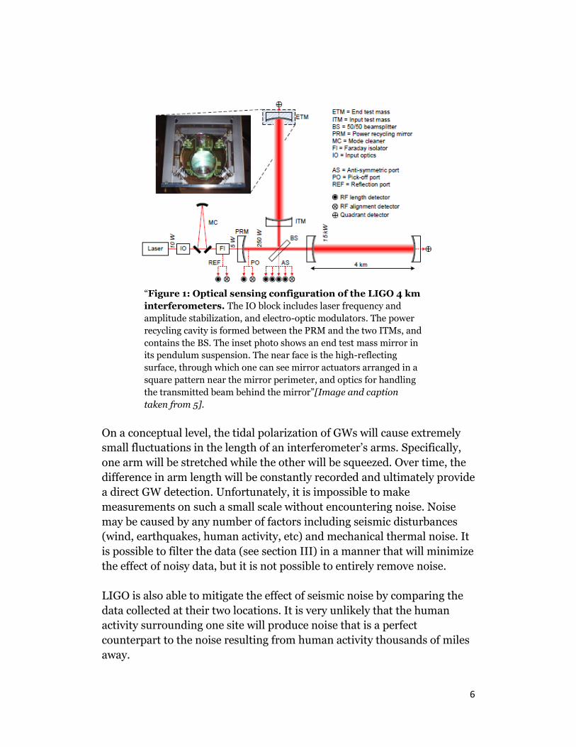
“Figure 1: Optical sensing configuration of the LIGO 4 km
interferometers. The IO block includes laser frequency and
amplitude stabilization, and electro-optic modulators. The power
recycling cavity is formed between the PRM and the two ITMs, and
contains the BS. The inset photo shows an end test mass mirror in
its pendulum suspension. The near face is the high-reflecting
surface, through which one can see mirror actuators arranged in a
square pattern near the mirror perimeter, and optics for handling
the transmitted beam behind the mirror”[Image and caption
taken from 5].
On a conceptual level, the tidal polarization of GWs will cause extremely
small fluctuations in the length of an interferometer’s arms. Specifically,
one arm will be stretched while the other will be squeezed. Over time, the
difference in arm length will be constantly recorded and ultimately provide
a direct GW detection. Unfortunately, it is impossible to make
measurements on such a small scale without encountering noise. Noise
may be caused by any number of factors including seismic disturbances
(wind, earthquakes, human activity, etc) and mechanical thermal noise. It
is possible to filter the data (see section III) in a manner that will minimize
the effect of noisy data, but it is not possible to entirely remove noise.
LIGO is also able to mitigate the effect of seismic noise by comparing the
data collected at their two locations. It is very unlikely that the human
activity surrounding one site will produce noise that is a perfect
counterpart to the noise resulting from human activity thousands of miles
away.
7
2.1.2 Compact Binaries
A compact binary consists of a two-star system with highly compact
bodies. The system may contain a pair of Neutron Stars (NS-NS), a
Neutron Star and a Black Hole (NS-BH), or two Black Holes (BH-BH).
These binaries will be locked in a cosmic dance of sorts as they slowly
converge. Compact binary coalescence occurs in three stages: inspiral,
merger, and ringdown.
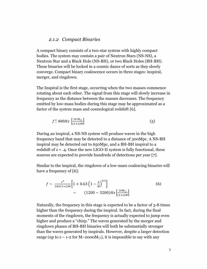
The Inspiral is the first stage, occurring when the two masses commence
rotating about each other. The signal from this stage will slowly increase in
frequency as the distance between the masses decreases. The frequency
emitted by low-mass bodies during this stage may be approximated as a
factor of the system mass and cosmological redshift [6].
[
] (5)
During an inspiral, a NS-NS system will produce waves in the high
frequency band that may be detected to a distance of 300Mpc. A NS-BH
inspiral may be detected out to 650Mpc, and a BH-BH inspiral to a
redshift of z = .4. Once the new LIGO-II system is fully functional, these
sources are expected to provide hundreds of detections per year [7].
Similar to the inspiral, the ringdown of a low-mass coalescing binaries will
have a frequency of [6]:
[ (
)
] (6)
[
]
Naturally, the frequency in this stage is expected to be a factor of 3-8 times
higher than the frequency during the inspiral. In fact, during the final
moments of the ringdown, the frequency is actually expected to jump even
higher and produce a “chirp.” The waves generated by the merger and
ringdown phases of BH-BH binaries will both be substantially stronger
than the waves generated by inspirals. However, despite a larger detection
range (up to z ~ 1-2 for M~2000M ), it is impossible to say with any

8
degree of certainty that these events will generate more detections than
inspirals. They are not as common and very little is known about the
merger stage of a BH-BH binary system.
Unfortunately, it is quite unlikely for the merger/ringdown of a NS-NS
system to fall within the sensitive range of laser interferometers. As such,
NS-NS systems will probably not provide much insight into the as yet
unknown NS equation of state.
However, it is possible for the immense tidal forces of a black hole in a NS-
BH binary to rip the NS apart before it even reaches the ringdown. This
phenomenon is known as the tidal disruption and will generate GWs out to
140Mpc that will enable the equation of state to be recovered!
2.1.3 Stellar Core Collapse
The formation of a type II supernovae and accretion induced collapse
(AIC) both provide prime candidates for the generation of detectable GWs.
However, the mechanism of these collapses is not well enough understood
to guarantee waves. It is very difficult to accurately model the degree of
asymmetry during a collapse. As detailed in section I, a symmetric body
lacks a quadrupole moment and will fail to produce GWs.
If the stars are spinning rapidly enough to generate an instability that
leads to asymmetry and GW emission, then the detection of waves
resulting from core collapse will provide insight into the mechanism of
collapse. Moreover, even if GWs from core collapse are not detected, their
absence will eventually provide insight into the nature of collapse as well.
EG once the lack of emission is not attributed to a lack of sensitivity, the
collapse may be assumed symmetric.
2.1.4 Periodic Emitters
The term Periodic Emitter most frequently refers to a Pulsar. Pulsars are
NS’s that rotate very rapidly with extreme phase precision. A non-
axisymmetric pulsar will have a quadrupole moment that is guaranteed to
generate gravitational waves. These waves will impact the PTA (EG Hulse-
Taylor, see section I).

9
The frequency of these pulsars is ~ 2(rotation frequency of NS). Therefore,
a rapidly rotating millisecond pulsar has the potential to be readily
detectable in the high frequency range. The amplitude of the waves
generated by pulsars may be derived from equation (2) after including the
prefactor. It will depend upon the inertia, I, and ellipticity, . [8]
(7)
The upper limit that has been proposed for ellipticity suggests that the
amplitude , which remains considerably beneath the current
threshold for detection. This limit raises a question. Why are pulsars
considered one of the most promising sources for GW detection in the next
5 years?
If a number of wave cycles may be coherently tracked, the signal may be
amplified by a factor ~ √ , where N represents the number of wave cycles
tracked. Although tracking cycles is extremely computationally expensive,
the process has been an ongoing project over the past 20 years. The
amalgamation of data is rapidly approaching a critical mass on the
imminent path to detection.
2.1.5 Stochastic Background
Waves from the stochastic background (SB) span a vast variety of
frequencies, but the amplitude of the GW background is decidedly smaller
than current ground-based detection capacities. Thus, the search for a
stochastic background of GWs involves merging the data sets of several
independent detectors and looking for recurring patterns in the noise.
Noise ought to be entirely random. As such, there should not be any
predictable correlation between the noise of data collected at different
locations. Any lapse in unpredictability (EG any noise correlation) that
may not be attributed to a global event (like a massive earthquake) would
provide evidence supporting the detection of a GW background.
The strength of any SB depends upon the energy density it contributes to
the universe as a fraction of the critical energy density required to close the
universe and halt expansion [9].
10
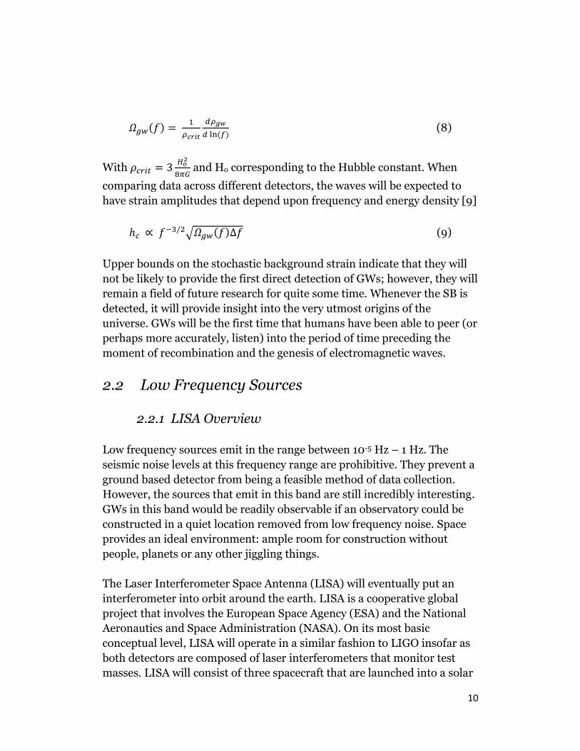
(8)
With
and Ho corresponding to the Hubble constant. When
comparing data across different detectors, the waves will be expected to
have strain amplitudes that depend upon frequency and energy density [9]
√ (9)
Upper bounds on the stochastic background strain indicate that they will
not be likely to provide the first direct detection of GWs; however, they will
remain a field of future research for quite some time. Whenever the SB is
detected, it will provide insight into the very utmost origins of the
universe. GWs will be the first time that humans have been able to peer (or
perhaps more accurately, listen) into the period of time preceding the
moment of recombination and the genesis of electromagnetic waves.
2.2 Low Frequency Sources
2.2.1 LISA Overview
Low frequency sources emit in the range between 10-5 Hz – 1 Hz. The
seismic noise levels at this frequency range are prohibitive. They prevent a
ground based detector from being a feasible method of data collection.
However, the sources that emit in this band are still incredibly interesting.
GWs in this band would be readily observable if an observatory could be
constructed in a quiet location removed from low frequency noise. Space
provides an ideal environment: ample room for construction without
people, planets or any other jiggling things.
The Laser Interferometer Space Antenna (LISA) will eventually put an
interferometer into orbit around the earth. LISA is a cooperative global
project that involves the European Space Agency (ESA) and the National
Aeronautics and Space Administration (NASA). On its most basic
conceptual level, LISA will operate in a similar fashion to LIGO insofar as
both detectors are composed of laser interferometers that monitor test
masses. LISA will consist of three spacecraft that are launched into a solar

11
orbit following the earth with a triangular configuration. The arm length
will change slowly and predictably throughout the course of orbit, but will
always remain approximately 5 million kilometers.
Figure 2: Artistic representation of LISA Mission (Left) and
orbital configuration of LISA (Right) Images taken from sources [3]
(left) and [9] (right).
A 5 million kilometer distance between spacecraft will cause diffraction to
spread the lasers. By the time that the laser reaches the detector, it will
have a diameter of ~20km. A small portion of this light is captured by the
detecting spacecraft. This light is then “interfered with a sample of light
from the on-board laser. Each spacecraft thus generates two interference
data streams.” [Excerpt taken from 9] The six resulting interference
streams are then combined in order to “construct the time variations of
LISA's armlengths and then build both gravitational-wave polarizations.”
[9] Modulating the amplitude of GW strain throughout the course of
LISA’s orbit around the sun will also supply the position of LF sources in
the sky.
Once launched, LISA will be able to verify the Kerr metric and No Hair
theory of BHs. It will facilitate a new degree of scrutiny into the nature and
development of massive BHs and has the potential to specify Dark Energy
(DE) parameters and discover new astronomical phenomena.
12
2.2.2 Coalescing Binary BHs
Although many coalescing binary systems will emit in the HF band, the
mergers of massive black holes (MBH) with roughly equal masses and
extreme mass ratio inspirals (EMRI) will emit at a lower frequency. LISA
will be able to detect MBH mergers out to a redshift z ~ 5-10. This is one
of the most exciting prospects of the mission
MBH mergers are only poorly understood. Observing their coalescence
will offer a wealth of information regarding the nature of black holes as
well as another opportunity to test gravity in its most extreme conditions.
Rate estimates for these events are estimated to be hundreds per year!
EMRI events will also be quite enlightening. The GWs from an inspiral of a
relatively small body (WD, NS, BH with mass 10 M ) into a MBH (mass
~ 105 – 107 M ) contain information regarding the geometry of space-time
during the event. Recovering this information will map the Kerr geometry
and enable the verification of the Kerr metric and No Hair theorem (EG
the theory stating that BHs are perfectly categorized by the mass and spin
because these are the only parameters that are not lost inside the void).
2.2.3 Periodic Emitters
Unlike the LIGO, LISA is actually guaranteed to detect GWs after its
launch. There are binary pulsar systems which are known to emit GWs
that fall well within LISA’s sensitivity band. In fact, at a frequency below ~
0.002 Hz, there will actually be too many binary systems to resolve. The
result will be a type of “noise” that is actually caused by GWs!
Frequencies above ~ 0.002 Hz will be scarce enough to be resolvable,
which is to say that the number of sources will be downscaled by a factor of
104-5 to ~ 104 detectable binaries. These binaries will facilitate the
generation of a 3D map of the binary systems in the galaxy that is not
impeded by dust.

13
2.2.4 Stochastic Background
The GWs present in the SB in the LF band are expected to be emitted by a
combination of primordial (EG Origin of the Universe) and astrophysical
events. One possible source of SB radiation is a phase change. The
frequency of GWs resulting from phase transitions are temperature
dependent and typically peak around
(
) (10)
Where T represents the temperature value and f is the peak frequency.
Using this, the waves resulting from the electroweak phase transition (EG
the moment at which the electric and weak forces began to differentiate) at
temperatures between T ~ 100-1000 could generate waves within the
sensitive band! [10]
Unlike the LIGO however, LISA will not be able to compare data collected
from multiple operation sites to the extent that there will only be one
spaced-based LF band detector. Although the primordial waves resulting
from inflation would be detectable in theory, they are likely to remain
below the noise levels. In light of the recent BICEP2 findings (higher than
anticipated amplitude of polarization), however, it does seem plausible
that LISA would find direct evidence of inflationary GWs.
2.3 VLF and ULF Sources
2.3.1 Very Low Frequency Pulsars
The VLF band covers frequencies from 10-9 Hz - 10-7 Hz and has not
received the amount of attention that the LF and HF bands have. This is
primarily because it proves much more difficult to study sources that emit
in this range. Neither ground-based nor space-based detectors prove
sufficient. Millisecond pulsars timing arrays actually constitute the main
detectors. VLF GWs resulting from SMBH inspirals and early-universe
phase transitions will cause small fluctuations in the arrival times of the

14
pulses. Once these fluctuations have been studied for long enough, then
information from the GWs may be recovered in a process somewhat
reminiscent of the Taylor-Hulse binary pulsar timing array described in
section I. VLF waves will help set limits on the stochastic background .
2.3.2 Ultra Low Frequency B-Mode Polarization
Recently, the publication of the BICEP2 findings has lent a lot of attention
to the ULF band. Waves in this range have frequencies between 10-18 Hz
and 10-15 Hz. They are the result of an inflationary epoch and oscillate on
“scales comparable to the size of the universe.” [Excerpt taken from 9]
ULF waves are studied indirectly through their polarization on the Cosmic
Microwave Background (CMB). Specifically, inflationary GWs are (roughly
speaking) the only source of helical B-mode polarizations on the CMB.
These waves would have been created (and amplified) during an
inflationary epoch such that the root mean square amplitude is
proportional to the energy scale of inflation
(
)
(11)
The BICEP2 findings claim to have detected B-mode polarization of light
in the CMB. More surprisingly, they hold that the tensor-scalar ratio r =
0.20. This is substantially larger than was anticipated. Assuming their
methodology withstands the scrutiny of the scientific community, the
scientists involved have provided the basis for detecting the “smoking gun
of inflation.”

15
3 Data Analysis
What is perhaps the most crucial piece of Gravitational Wave Astronomy does
not occur until after the data has all been collected. The process of data analysis
takes a series of noisy oscillations and turns it into information about the past
and present universe. Unfortunately, the random nature of noise makes it
impossible to ever declare detection with 100% certainty. There will always
remain some possibility that random noise has conspired to look like a very
convincing signal. When studying GWs, it is therefore crucial for the scientific
community to agree upon some degree of significance. Eventually, with a high
enough degree of significance the uncertainty will become small enough to be
considered negligible. Consider, for example the hypothetical case wherein a
signal has been generated which would only be duplicated by noise once every
10 million years. It is so incredibly unlikely that any particular instance is noise
that detection would be almost certain!
3.1 Detection Probability
3.1.1 Significance and Confidence
Statistically speaking, the process of testing for a signal is very similar to setting
significance (α-value) or constructing a confidence interval during hypothesis
testing. The false alarm probability is synonymous with significance and
corresponds to the probability that random noise has generated a passable
signal. The Probability Density Function (PDF) of a false detection is given by
[11]
∫
(12)
While confidence may be calculated quite simply by considering 1-Pf(R) where R
Rcomplement spans all possible values of x. Similarly, the probability of a
detection is given by [11]
∫
(13)
3.1.2 Χ2 Likelihood and Goodness of Fit Test
Typically, datasets from ground based interferometers like LIGO may be
approximated as having stationary, normally distributed noise such that the

16
expectation values for the mean and mean-square levels of noise in the absence
of a signal are given respectively by [12]
[ ] [ ] (14)
[
[ ] (15)
Where the expectation value is defined according to the standard definition in
both the discrete and continuous cases
[ ] ∑ (16)
[ ] ∫
(17)
E[|n|2] depends upon “the one-sided noise spectral density at frequency f, Sn(f),
and the observation time, T” [Excerpt taken from 12]. If a signal were in fact
present, the signal stream s(t)=R(t,τ)h(τ) + n(t) where the first term no longer
vanishes. The likelihood test (19) in this case simply becomes an expression of
the Χ2 test (17) that describes the goodness of fit of a model [12, 13,16]
∑
(17)
Where the likelihood test is given by the inner product [12]
∑
(18)
Such that the likelihood may be found after accounting for the prefactor by the
exponential of a chi-squared test [12]
(19)
With the residual r = s - R h.
3.1.3 – Neyman-Pearson Approach
Statistically, the Neyman-Pearson Approach (NPA) may be interpreted as a kind
of trade-off between type I and type II error. Error occurs in hypothesis testing

17
when the wrong conclusion regarding the null hypothesis (H0) is reached.
Specifically, type I error occurs when H0 is wrongly rejected while type II error
occurs when H0 is wrongly favored. NPA typically examines the ratio between
probability of detection and significance [13]
(20)
A threshold value will be set using this ratio to determine the minimum criteria
for detection.
3.2 Filtering
3.2.1 Constant Frequency Fourier Transform Filter
Before performing statistical detection testing, the data must be filtered in a
manner that will remove noise without disturbing the desired signal. This is
predictably tricky and depends heavily upon the distribution of the noise and
the nature of the signal. It is, therefore, especially difficult to filter adequately
when the signal has never been detected before! If the data is expected to
contain a signal of constant albeit unknown frequency, then a simple Fourier
Transform (FT) of the signal will suffice [11,13]
∫
(21)
With:
The Fourier domain will rearrange a signal of constant frequency such that the
noise is evenly distributed across the entire spectrum while the power of the
signal is all stacked upon a single frequency. After detecting the source in the
Fourier domain, it may be reverted by applying the standard inverse FT
∫
(22)
Unfortunately, this filter is largely insufficient. Although most sources will emit
at a constant frequency, the orbital motion of detectors will produce a Doppler
shift on the arriving waves. It was included here as a simple introduction into
the conceptual realm of filtering.

18
3.2.2 Matched Filtering in Zero-Mean Gaussian Noise
In reality, noise will not be a perfectly zero-mean Gaussian; however, the
approximation is not terrible and the assumption will suffice for the purposes of
this section. The predominant method for categorizing noise (especially
Gaussian noise) is defined simply by taking the expectation value of the noise at
two distinct times. It is referred to as the autocorrelation function [11, 13]
[ ] (23)
The matched filter (MF) q(t’) for an expected signal s(t) depends upon the time
evolution of the signal and may be calculated by solving [11, 13]
∫
(24)
for a given set of parameter values. The expected value of s(t) that is input into
this equation is generally referred to as the template of a filter. This will be
discussed further in section 3.2.3.
If the data is observed continuously over some time interval then the logarithm
of the likelihood function will depend upon the time evolution of the matched
filter, expected signal, and observed data set [11, 13]
[ ] ∫
∫
(25)
With the total observed data set occurring as the additive superposition of the
noise and the signal [11, 12, 13]
(26)
Equation (25) may be simplified by noticing that only the first term actually
depends upon the collected data set. As such, the second term may be
successfully incorporated as a constant given a set of parameters and an
observational window. The important ratio depends only upon a the detection
statistic [11, 13]
∫
(27)
If the detection statistic surpasses a given threshold G0 according to the process
described in section 3.1, then detection may be claimed. Although the

19
calculations are outside the scope of this paper, it ought to be mentioned that in
the case of stationary noise such that K(t, t’) depends only upon time differences
and the matched filter calculations are simplified
enough to be exactly analytically calculable by the use of FT techniques. Refer to
[13] for a review of this process. The final solution that falls out for the FT of the
matched filter depends upon the one-sided noise spectral density and the FT of
the template selected
(28)
Where Sn is only defined for the set of non-negative frequencies. Increasing the
noise density within a filter will directly decrease the filter’s contribution to the
detection statistic. This resonates intuitively. Higher noise levels make detection
less probable.
3.2.3 Templates
Template construction is an extremely important part of the process of data
analysis. The process of generating a template is typically a combination of
analytic and numerical approximations based on assumptions about parameters.
Searching data via templates can be a very effective method of raising signals
out of the noise. Generally, a single template will prove to be insufficient, but
after constructing the number of templates required, a given search will be
orders of magnitude more efficient.
The efficiency of a search depends largely upon the number of parameters that
the analysis must track. Using a well-constructed template-based model allows
the search to account for far fewer parameters.
Numerically, consider the example of the search for a binary NS-NS inspiral.
Evidence has shown that the signal may be coherently tracked over N ~ 10,000
cycles. This will amplify the signal by a factor of ~ 100 (see section 2.1.4: EG √
dependence of amplification). Detection by the use of a general model requires
an integrated SNR > 100 [12] which implies an absolute S/N ratio > 1. The use
of a template-based model only requires an integrated SNR > 7 for detection [12]
This means that an absolute S/N ratio > 7/100 ~ S/N > 0.07 will suffice!
Although the use of templates has the potential to greatly increase the
confidence of a given data set, it is absolutely essential to select an accurate
template. Template-based models force a search to select between a signal that

20
matches the given amplitude no signal. Thus, a faulty template would
automatically eliminate the possibility of detection. Moreover, if the template
s(t) in a matched filter has miscalculated the phase of a signal, then the template
will cause a destructive interference that proactively reduces the sensitivity of
the filter. Even if the amplitude is accurate, phase error makes detection
exceedingly unlikely. When employing the use of a template-based model, note
that the model will be much more sensitive to phase error than amplitude error.
3.2.4 Nyquist Theorem and Aliasing
The Nyquist theorem is actually quite straightforward. It sets a lower bound on
the required sampling interval. If data is sampled at intervals of Δt, then the
sampling rate will naturally be 1/Δt. The maximum frequency that can
physically be observed in this time is bounded by f = 1/2Δt. In other words, the
sampling rate may be truncated at a value of 2f. This truncation will prevent the
noise from higher frequencies from inadvertently being mapped down and
contributing to the noise levels of the observation band. Refer to [11] for the
formal development of this concept.
3.2.5 Maximum Likelihood Estimator
When a signal is analyzed, the process frequently seems to resemble
orienteering without a map on a foggy night. An eventually successful pioneer
must tolerate repeated experimentation and, frequently, some degree of
guesswork that has its basis in past failures. More concretely, the waveform of a
signal is often only known as a function of unknown parameters. Signal
amplitude and time of arrival (TOA), chirp mass, and arrival phase are all rarely
known parameters. The Maximum Likelihood Estimator (MLE) for a given set
of parameters is found by choosing the parameters in a manner that maximizes
the parameter-dependent likelihood ratio. This is given by an equation that is
easily motivated by the likelihood ratio presented in the Neyman-Pearson
Approach (C.f. equation 20).
(29)
Similarly, the filter and detection statistic (C.f. equations 27, 28) will also have
parameter-dependent analogs:
(30)

21
∫
(31)
In order to find the MLE for m unknown parameters, an m-dimensional grid
populated with discrete parameter values must be solved. Effectively, this will
constitute a standard optimization problem from calculus in which the
derivatives of m equations are simultaneously set to zero in order to solve for
the critical points
[ ] (32)
The process of solving an m-dimensional grid very quickly becomes expensive
in multiparameter problems.
3.2.6 Bayesian Inference
The development of Bayesian data analysis algorithms is a rapidly emerging
field of study. At present, there is not a fully developed procedure detailing the
Bayesian approach to data analysis. Currently, Bayesian Inference (BI) is
primarily used as a supplement to improve upon the well-established search
algorithms (Notably MFs and MLEs). The approach functions by prescribing a
cost to every decision that is made and then discerning the posterior
distribution (EG the conditional probability of an event after accounting for
relevant factors) of a model from the prior probability of the model and the
marginal likelihood of the model.
The first step in Bayesian analysis is to compute/approximate the marginal
likelihood and the prior. This is done by assessing and calculating various Bayes
Risk factors. While important, the process is tedious and rather lengthy and
may be seen in section 3 of [13].
After calculating these values, they posterior probability of a model is given by
[14, 15]
(33)
Where pr(s) is the normalization factor that could theoretically be obtained by
integrating [15]

22
∫
(34)
However, this integration is problematic and expensive at best, and unsolvable
at worst. Fortunately, it may be skirted by considering the relative probability of
two models. Let Mi denote the model claiming the presence of a GW signal
within the noise. Similarly, let Mj refer to the model claiming the absence of any
GW signal. The ratio of the two is given by [14]
(35)
Defining the product of prior belief [14]
(36)
And the Bayes factor [14]
(37)
The ratio may be abbreviated as the product of prior belief and the Bayes factor
[14]
(38)
3.2.7 A (Very) Brief Introduction to MCMC Methods
Although Markov Chain Monte Carlo Methods (MCMC) are too intricate to
sufficiently summarize in this paper, their relation to Bayesian Inference is
fairly straightforward. MCMC methods require a likelihood, prior, and proposal.
Defining a likelihood function is not often an easy task. In the case of Gaussian
noise, it may be derived by applying Bayesian analysis to a matched filter. The
result is an application of equation (19).
First, recognize that “the conditional probability of measuring [data set] s(f)
when a signal h(f) is present, is equal to the conditional probability of
measuring [data set] s0 = s(f)−h(f) assuming that no signal is present” [excerpt
taken from 14] such that
(39)

23
In other words, subtracting the signal from a data set with said signal present
ought to give a data set with no signal present. Although it is easy to get turned
around in the words, the end result of substituting conditional probabilities and
applying the definition of an inner product from (18) will look very similar to (19)
(40)
Values for the priors required are typically well understood and may be
approximated by well-accepted literature values. The proposal distribution
must be selected carefully in a way that does not take a prohibitively long
amount of time to produce a stationary distribution that provides an accurate
approximation of the posterior distribution.

24
4 Summary
Gravitational Wave Astronomy is one of the most exciting fields of study to
emerge in the past century. In the imminent future, their detection will enable a
galactic array of insight into astrophysical phenomena including: the nature of
gravity and relativity, the process by which compact binary systems (NS-NS,
NS-BH, and BH-BH) coalesce, the nature of dark energy, the opening seconds of
the universe before recombination, the process of early-universe phase
transitions, the nature of black holes, the NS equation of state, and possibly the
process by which stellar bodies collapse, not to mention the potential for
discovering entirely new, unobserved phenomena. Despite abundant, nearly
overbearing obstacles complicating data collection and analysis, a global
coalition of the world’s brightest minds is rapidly overcoming every
complication and racing toward a new era of astrophysics.
The detection and characterization of gravitational waves will be comparable
to a “baby using ultrasound from inside the womb to observe the world
outside” (N. J. Cornish, 2014).

25
Acknowledgements:
[1] B. F. Schutz (1997), gr-qc/9710079
[2] T. Creighton, Quadrupole moment, http://www.tapir.caltech.edu
[3] J. Baker et al (1997), LISA-LIST-RP-436, vol. 1, pp 1-117.
[4]K. J. Lee (2014), arXiv:1404.2090
[5] B. Abbot et al (2007), arXiv:0711.3041v1 [gr-qc]
[6] E. E. Flanagan and S. A. Hughes, Phys. Rev. D 57 (1998), 4535.
[7] C. Cutler and K. S. Throne (2002), gr-qc/0204090
[8]N. J. Cornish and J. B. Camp (2004). Annu. Rev. Nucl. Part. Sci. 54:525–77
[9] S. A. Hughes (2003), Annals Phys. 303 (2003) 142-178
[10] D. Sticlet (2009). Phase Transitions in the Early Universe
[11] B. F. Shutz (1997), gr-qc/9710080
[12] N. J. Cornish (2013), Phil. Trans. R. Soc. A. 371, 20110540
[13] P. Jaranowski and A. Krolak (2009), Cambridge University Press
[14] N. J. Cornish (2009), Cambridge University Press
[15] C. Andrieu, N. D. Freitas, A. Doucet, and M. I. Jordan (2003). Machine
Learning, 50, 5–43
[16] Chi-Squared Goodness of Fit Test (1997), http://www.stat.yale.edu


