27 July 2006 Pupil planes versus Image planes 1

Pupil Planes versus Image PlanesPupil Planes versus Image PlanesComparison of beam combining conceptsComparison of beam combining concepts

John YoungUniversity of Cambridge

27 July 2006 Pupil planes versus Image planes 2

OutlineOutline• Aims of this presentation• Beam combiner functions• Image plane vs Pupil plane• Multiplexing multiple baselines

– Cross-talk

• Field of View Issues• Summary

27 July 2006 Pupil planes versus Image planes 3

Aims of PresentationAims of PresentationI am aiming to get across the following:• Common features of image plane and pupil plane combination• Differences• Trades-off in combiner design• Some instrument-related issues in interpreting visibility data

27 July 2006 Pupil planes versus Image planes 4

Beam Combiner FunctionsBeam Combiner Functions• Generate fringe pattern(s) suitable for recording with detectors• Want fringes on many interferometer baselines

– Amplitude and phase of fringes on each baseline encode amplitude and phase of one Fourier component of source brightness distribution

• Want high-signal-to-noise fringes– Small collectors, low throughput; hence few photons– Atmosphere usually forces short integration times

• Since we cannot coherently amplify our signals, the previous tworequirements usually conflict

27 July 2006 Pupil planes versus Image planes 5

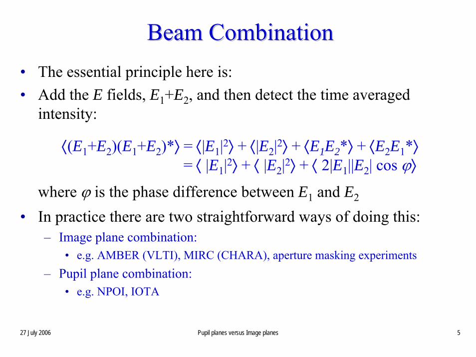
Beam CombinationBeam Combination• The essential principle here is: • Add the E fields, E1+E2, and then detect the time averaged

intensity:

⟨(E1+E2)(E1+E2)*⟩ = ⟨|E1|2⟩ + ⟨|E2|2⟩ + ⟨E1E2*⟩ + ⟨E2E1*⟩= ⟨ |E1|2⟩ + ⟨ |E2|2⟩ + ⟨ 2|E1||E2| cos ϕ⟩

where ϕ is the phase difference between E1 and E2

• In practice there are two straightforward ways of doing this:– Image plane combination:

• e.g. AMBER (VLTI), MIRC (CHARA), aperture masking experiments– Pupil plane combination:

• e.g. NPOI, IOTA

27 July 2006 Pupil planes versus Image planes 6

Image Plane (MultiImage Plane (Multi--Axial) CombinationAxial) Combination• Mix the signals in a focal

plane as in a Young’s slit experiment:

• In the focused image the transverseco-ordinate measures the delay

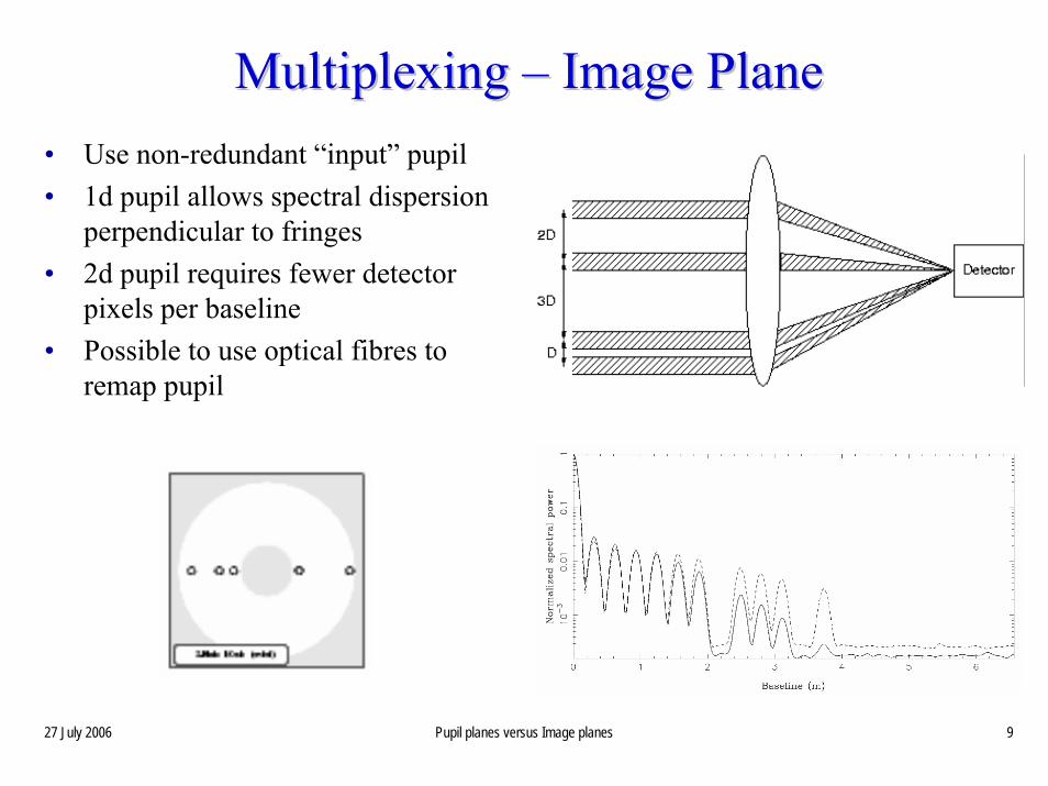
• Fringes encoded by use of a non-redundant “input” pupil

• Possible to use dispersion prior todetection in the direction perpendicular to the fringes

27 July 2006 Pupil planes versus Image planes 7

Pupil Plane (CoPupil Plane (Co--Axial) CombinationAxial) Combination• Mix the signals by superposing afocal beams:• Focus superposed beams onto a

single element detector

• Fringes encoded by use of a non-redundant modulation of delay of each beam

• Fringes are recorded by measuring intensity versus time

• Spectral dispersion can be used prior to detection

27 July 2006 Pupil planes versus Image planes 8

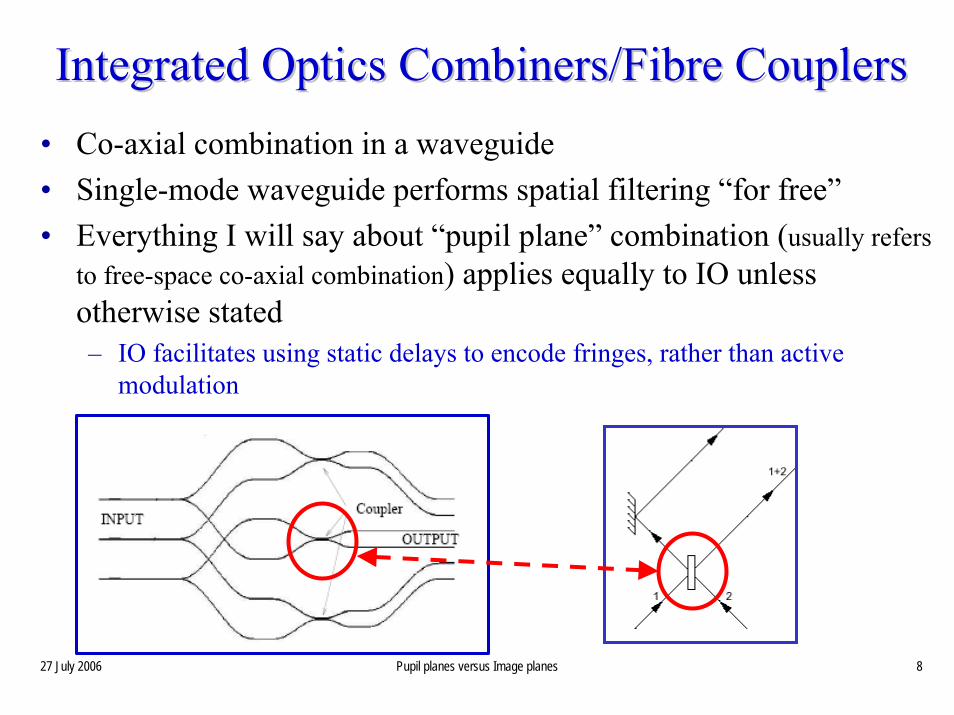
Integrated Optics Combiners/Integrated Optics Combiners/FibreFibre CouplersCouplers• Co-axial combination in a waveguide• Single-mode waveguide performs spatial filtering “for free”• Everything I will say about “pupil plane” combination (usually refers

to free-space co-axial combination) applies equally to IO unless otherwise stated– IO facilitates using static delays to encode fringes, rather than active

modulation

27 July 2006 Pupil planes versus Image planes 9

Multiplexing Multiplexing –– Image PlaneImage Plane• Use non-redundant “input” pupil• 1d pupil allows spectral dispersion

perpendicular to fringes• 2d pupil requires fewer detector

pixels per baseline• Possible to use optical fibres to

remap pupil

27 July 2006 Pupil planes versus Image planes 10

Multiplexing Multiplexing –– Pupil PlanePupil Plane• Mix beams at successive beam-

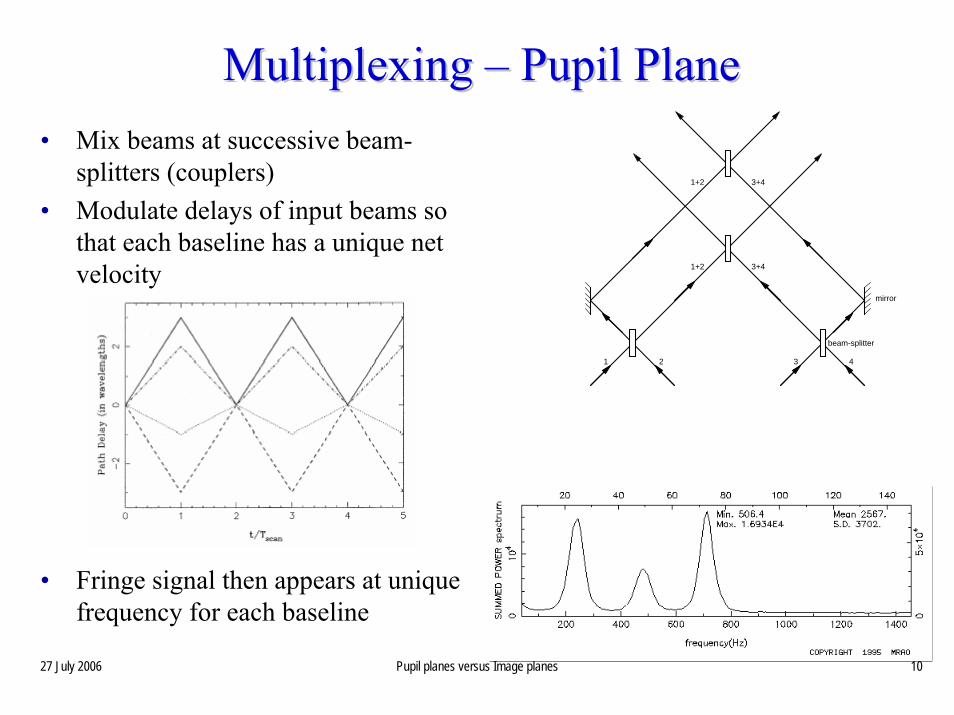
splitters (couplers)• Modulate delays of input beams so

that each baseline has a unique net velocity

• Fringe signal then appears at unique frequency for each baseline

3 4

1+2 3+4

1+2

1

3+4

2

beam-splitter

mirror

27 July 2006 Pupil planes versus Image planes 11

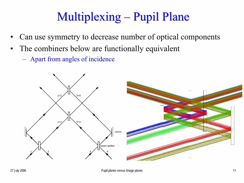
Multiplexing Multiplexing –– Pupil PlanePupil Plane• Can use symmetry to decrease number of optical components• The combiners below are functionally equivalent

– Apart from angles of incidence

3 4

1+2 3+4

1+2

1

3+4

2

beam-splitter

mirror

27 July 2006 Pupil planes versus Image planes 12

SignalSignal--toto--Noise ComparisonNoise Comparison• Buscher (1988) showed that (all-one-one) pupil-plane and image-

plane implementations give identical signal-to-noise, provided:– Noise-free detector– Fringe scanned in << t0

– Can coherently combine signals from all outputs of pupil-plane combiner

• Choice driven by practical considerations– Detector format & performance– Cost of detector(s)– Cross-talk/calibration– Alignment/stability– Spectral bandwidth

27 July 2006 Pupil planes versus Image planes 13

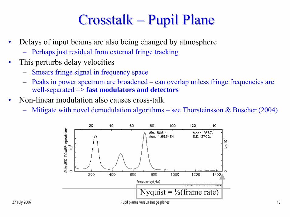
Crosstalk Crosstalk –– Pupil PlanePupil Plane• Delays of input beams are also being changed by atmosphere

– Perhaps just residual from external fringe tracking• This perturbs delay velocities

– Smears fringe signal in frequency space– Peaks in power spectrum are broadened – can overlap unless fringe frequencies are

well-separated => fast modulators and detectors• Non-linear modulation also causes cross-talk

– Mitigate with novel demodulation algorithms – see Thorsteinsson & Buscher (2004)

Nyquist = ½(frame rate)

27 July 2006 Pupil planes versus Image planes 14

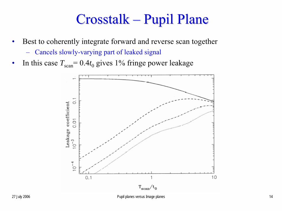
Crosstalk Crosstalk –– Pupil PlanePupil Plane• Best to coherently integrate forward and reverse scan together

– Cancels slowly-varying part of leaked signal• In this case Tscan= 0.4t0 gives 1% fringe power leakage

27 July 2006 Pupil planes versus Image planes 15

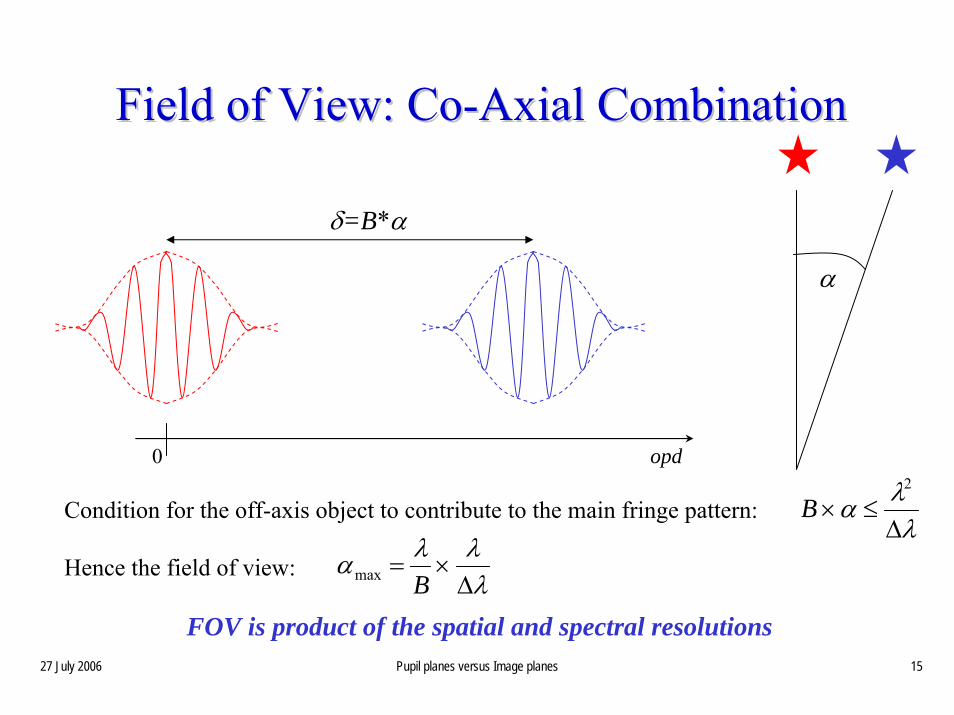
Field Field ofof ViewView: : CoCo--AxialAxial CombinationCombination

opd0

δ=B*α

Condition for the off-axis object to contribute to the main fringe pattern:

Hence the field of view:

FOV is product of the spatial and spectral resolutions

B ×α ≤λ2

Δλαmax =

λB×

λΔλ

α

27 July 2006 Pupil planes versus Image planes 16

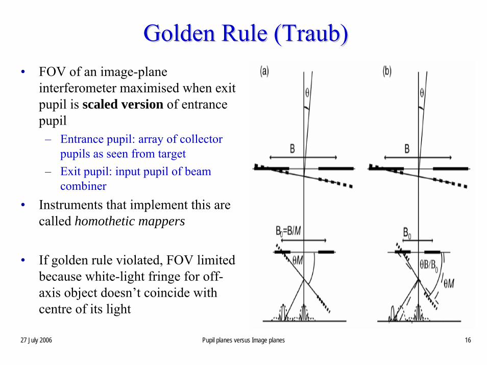
Golden Rule (Golden Rule (TraubTraub))• FOV of an image-plane

interferometer maximised when exit pupil is scaled version of entrance pupil

– Entrance pupil: array of collector pupils as seen from target

– Exit pupil: input pupil of beam combiner

• Instruments that implement this are called homothetic mappers

• If golden rule violated, FOV limited because white-light fringe for off-axis object doesn’t coincide with centre of its light

27 July 2006 Pupil planes versus Image planes 17

Homothetic Mapping: How ToHomothetic Mapping: How To• Easy way

– Collectors on common mount– e.g. aperture masking, LBT

• Hard way– Collectors on independent mounts– Active relay optics to continuously adjust pupil mapping as Earth rotates– e.g. ……

27 July 2006 Pupil planes versus Image planes 18

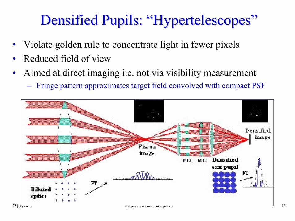
DensifiedDensified Pupils: Pupils: ““HypertelescopesHypertelescopes””• Violate golden rule to concentrate light in fewer pixels• Reduced field of view• Aimed at direct imaging i.e. not via visibility measurement

– Fringe pattern approximates target field convolved with compact PSF

27 July 2006 Pupil planes versus Image planes 19

FOV LimitsFOV Limits• Need to consider which of following give rise to FOV lower limit

for each baseline of each observation:– FOV of collectors– Isoplanatic patch– FOV of interferometer optical train– Beam Combiner configuration – OPD effects– Spatial Filters

• For a dilute-aperture array, the above list is usually in order of decreasing FOV– Exchange the last two for lower spectral resolutions

• Remember that only the Fourier components corresponding to your projected baselines are sampled– Cannot image fields with many filled pixels unless many collectors

27 July 2006 Pupil planes versus Image planes 20

InterferometricInterferometric (coherent) versus incoherent FOV(coherent) versus incoherent FOV

• In general, FOV over which target will contribute to measured fringe power (correlated flux) ≠ FOV for detected incoherent flux

• Visibility amplitude est. is ratio of coherent to incoherent flux:

• Incoherent field ≥ coherent (interferometric) field– Each part of field can contribute just DC signal, or both DC and fringe

power, or not at all• Centres of coherent and incoherent fields may not coincide

precisely e.g. if target has non-uniform colour– Centre of coherent field related to fringe-tracking centre– Centre of incoherent field related to guiding centre

27 July 2006 Pupil planes versus Image planes 21

FOV Limits (again)FOV Limits (again)• Need to consider which of following give rise to FOV lower limit

for each baseline of each observation:– FOV of collectors – limits incoherent field– Isoplanatic patch – limits coherent field– FOV of interferometer optical train – limits incoherent field– Beam Combiner configuration (OPD effects) – limits coherent field– Spatial Filters – limits incoherent field

• For a dilute-aperture array, the above list is usually in order of decreasing FOV– Exchange the last two for lower spectral resolutions

27 July 2006 Pupil planes versus Image planes 22

Restricted FOV effectsRestricted FOV effects• Some examples:

– coherent FOV = incoherent FOV < target sizeInterferometer “sees” smaller target => overestimates visibility

– coherent FOV < target size < incoherent FOVExtra incoherent flux reduces visibility => net under- or overestimate

• Remember effects will have different magnitude on different baselines, so data need careful interpretation

27 July 2006 Pupil planes versus Image planes 23

Summary: Pupil planes versus Image planesSummary: Pupil planes versus Image planes

Image Plane Pros:– Allows homothetic configuration to

access larger fields

Image Plane Cons:– Need large format detectors– Usually need highly anamorphic

optics to realise spectral resolution

Pupil Plane Pros:– Fewer detector pixels needed

Pupil Plane Cons:– Need fast modulators, fast detectors– Cross-talk– Potentially many optical

components (not with IO or contacted optics)