V2 Oct 2013 T. Tyson 1

PHYSICS 123/253 Thermal Johnson Noise Generated by a Resistor

Complete  Pre-­‐Lab  before  starting  this  experiment  

HISTORY In 1926, experimental physicist John Johnson working in the physics division at Bell Labs was researching noise in electronic circuits. He discovered that there was an irreducible low level of noise in resistors whose power was proportional to temperature. Harry Nyquist, a theorist in that division, got interested in the phenomenon and developed an elegant explanation based on fundamental physics.

THEORY OF THERMAL JOHNSON NOISE

Thermal agitation of electrons in a resistor gives rise to random fluctuations in the voltage across its terminals, known as Johnson noise. In Problem 1, you are to show that in a narrow band of frequencies, fΔ , the contribution to the mean-squared noise voltage from this thermal agitation is, 2( ) 4 Btime

V t Rk T f= Δ (1)

where R is the resistance in ohms and T is the temperature in degrees Kelvin for the resistor, Bk is the Boltzmann constant ( 231 38 10−. × J/K). This voltage is too small to be detected without amplification. If the resistor is connected across the input of a high-gain amplifier whose voltage gain as a function of frequency is ( )G f , the mean square of the voltage output of the amplifier will be: 2 2 2

0( ) 4 [ ( )] ( )out B Ntime time

V t Rk T G f df V t∞

= +∫ (2)

where 2( )N time

V t is the output noise generated by the amplifier itself.

Thus by measuring 2( )out time

V t as a function of R and making a plot, one obtains

2

04 [ ( )]Bk T G f df

∞

∫ from the slope, while the abscissa gives 2( )N timeV t . But the

amplifier gain ( )G f can be independently measured and the gain integral 2

0[ ( )]G f df

∞

∫

evaluated. The slope will then give a value for the Boltzmann constant Bk .

V2 Oct 2013 T. Tyson 2

This is in outline the first part of the experiment. The second part involves measuring the noise voltage as a function of the temperature, to verify the expected temperature dependence.

Problem 1 - Derivation of Eq. (1)

An electrical transmission line connected at one end to a resistor R and at the other end by an "equivalent" resistor R may be treated as a one-dimensional example of black body radiation.

Figure 1. Two resistors (of equal resistance R) coupled via a transmission line. At finite temperature T , the resistor R generates a noise voltage ( )V t which will propagate down the line. If the characteristic impedance of the transmission line is made equal toR , the radiation incident on the "equivalent" resistor R from the first resistor R should be completely absorbed. The permitted standing wave modes in the line have 2L nλ = / and ( 2 )f c L n= / , where

1 2 3n = , , , etc., and v is the wave velocity in the line. The separation of the modes in frequency is 2v L/ , mode density σ, and the number of modes between f and f f+Δ is ( ) (2 )f f L c fσ Δ = / Δ (3) From the Planck distribution or the equipartition theorem, the mean thermal energy contained in each electromagnetic mode or photon state in the transmission line is:

( )1B Bhf k T

hfE f k Te /= ≈

− at low frequencies. (4)

V2 Oct 2013 T. Tyson 3

From Eq. (3) and (4) find the electromagnetic energy ( ) ( )E f f fσ Δ in a frequency interval fΔ . One half of this energy is generated by the first resistor of R and propagating towards the "equivalent" resistor R . Knowing the propagation time from the generating resistor to the absorbing resistor t L cΔ = / , show that the absorbed power by the "equivalent" resistor R equals ( ) BP f f k T fΔ = Δ . (5)

In thermal equilibrium, this power is simply the ohmic heating generated by a noise voltage source ( )V t from the first resistor. Since ( )V t is terminated by the absorbing resistor R and has an "internal" resistance R (the first resistor), it produces a current

(2 )I V R= / in the line. Hence the power absorbed by the "equivalent" resistor R over the frequency interval fΔ can also be calculated as

2 2 2

2 ( )2 4 4V V V f fI R RR R R

Δ⎛ ⎞= = =⎜ ⎟⎝ ⎠

(6)

By equating ( ) BP f f k T fΔ = Δ to

2

V f RΔ / , show that 2 ( ) 4 BV f f k TR fΔ = Δ (7)

and 2( ) 4 Btime

V t k TR f= Δ (8)

This is known as Nyquist’s theorem as shown in Eq. (1). The power spectral density (noise power per unit frequency) is independent of frequency. Most other noise sources in nature have a f -1 to f -2 spectrum. Question: what is the integrated power of this Johnson noise over all frequencies? [i.e., why can’t a single resistor supply the world’s energy needs?] Eq. (1) is interesting: the left hand side describes random fluctuations of a lossy system in thermodynamic equilibrium. i.e. it is an equilibrium property; both the electrons and the lattice are in equilibrium at some temperature T. However, the right hand side of the equation refers explicitly to a non-equilibrium property of the same lossy system: the resistance R, which is measured by applying a voltage (taking the system out of equilibrium) and measuring the current of electrons scattering through the lossy system. Johnson noise is an example of a broader fundamental principle in nature called the “fluctuation-dissipation theorem.” It relates the non-equilibrium dissipation in a system to its spontaneous fluctuations in equilibrium. See accompanying papers by Callen. RESISTOR  AND  APPARATUS  

V2 Oct 2013 T. Tyson 4

You   have   several   resistors   for   your   source   of   noise:   a   box  with  many   resistors   at   room  temperature  (switch  selected).    [For  those  doing  this  as  their  main  experiment,  you  also  have  a  resistor  connected  at  the  end  of  parallel  wire  leads  in  a  tube.  The  resistor  is  thermally  connected  to  the  bottom  of  the  tube  with  some  glue.    The  wire  leads  are  thin  so  they  don’t  conduct  much  heat;  this  is  so  that  the  resistor  at  the  end  of  the  tube  will  cool  to  the  temperature  of  the  bottom  plate  when  cooled.]      A  very  low  noise  operational  amplifier  is  used  as  the  first  stage  of  amplification  for  the  Johnson  noise.  This  preamp  has  a  built-­‐in  band  pass   filter:  ~200  Hz   to  1800  Hz.  Beware:   the   filter  built  into   the   amplifier   is   only   one   component   in   the   effective   gain   vs   frequency   behavior   for   this  system:   the  small  “parasitic”  capacitance   in  parallel  with   the  resistor   is  a   filter   in   its  own  right  (you  must   account   for   this   if   you   use   resistances   near   a  megohm).     The   resulting   “filter”   is   a  product   of   the   RC   filter   on   the   input   (small   high   frequency   roll-­‐off)   and   the   rather   square  bandpass  filter  in  the  amplifier  box.  The  apparatus  is  connected  with  shielded  coaxial  cables  as  shown   to   reduce   pickup.   Beware:   there   is   a   special   easily   damaged   3-­‐wire   connector   on   the  amplifier  input  that  looks  like  a  BNC,  but  it  is  not.  Do  not  twist  this  input  connector.       The  sine  wave  oscillator   is  used   to  measure   the  gain  vs   frequency  of   the  amplifier.    The  oscillator   output   is   put   through   an   attenuator   to   reduce   it   to   the   level   needed   to   be   able   to  insert  into  the  amplifier.    The  attenuation  factor  is  accurately  given  by  the  controls  and  does  not  need  to  be  calibrated.    Check  its  output  voltage  before  directly  connecting  to  the  amplifier  input.    The   frequency   f   of   the   oscillator   can   be   accurately   set   and   determined   with   the   Integrating  Digital  Voltmeter.    Finally,  you  have  a  spectrum  analyzer.  

V2 Oct 2013 T. Tyson 5

In addition to the resistors (box and cold probe) and the low noise bandpass amplifier shown above, you have all the equipment you need (and more!) to design your experiment and make the necessary measurements, including calibration. Shown above (left to right): HP 5315 Frequency counter Agilent 34401A Digital precision volt meter (AC or DC) HP 204D Oscillator HP350D Attenuator Power supply for the low noise band pass amplifier Tektronix 2205 Oscilloscope Computer with software for PicoScope and data analysis software PicoScope 4262 Digital scope and spectrum analyzer (off photo to right) See http://www.picotech.com/applications/resolution.html

V2 Oct 2013 T. Tyson 6

We recommend that you first begin this measurement by making an approximation for the integral of the gain squared over frequency. Look at the spectrum on the PicoScope [instructions below] and make an approximation for an equivalent square bandpass. See also the linear plot of the gain shown below. Use that fΔ as the equivalent bandpass in

the equation for Johnson noise. To get the gain of the amplifier, inject a small amplitude sine wave as a calibrator as described in the next section and measure the output. Use the RMS AC voltmeter in all these measurements. With some care you should be able to get the Boltzmann constant to better than 20% accuracy in this way. A more accurate measurement involves integrating over the squared gain [since you are measuring squared voltage, or power] as described in the next section. PROCEDURE FOR MEASURING THE GAIN INTEGRAL [G(f)]2

0

∞

∫ df

You obtain [G(f)]2

0

∞

∫ df by measuring the amplifier gain G(f) at a discrete

and evenly spaced set of frequency values (f) and then evaluating the discrete

sum [G(f)]2∑ Δf numerically. You measure the gain G by injecting a known

voltage to the amplifier and then measuring its output voltage. But: the amplifier takes only VERY small input voltages!! Keep input under 250 microV.

To measure G(f), connect a precision broadband voltage attenuator to the input of the amplifier. The attenuator is used to assist you in determining the amplifier gain G(f) as follows. Supply the input of the attenuator with a sinusoidal voltage signal of Vi = 1 volt at some frequency between zero and 3000 Hz. For the best accuracy, measure the applied voltage signal with a digital rms voltmeter. Since at f = 1000 Hz, G(f) is roughly 10000, you can set the attenuation parameter NdB ~ 80 dB that gives a voltage attenuation factor of GA = 10NdB 20 ~ 10000). The output of the

V2 Oct 2013 T. Tyson 7

attenuator, Vi GA , is then fed into the input of the amplifier. You measure the amplifier output Vo = Vi GA( )G f( ) with the same rms voltmeter. The amplifier gain is given by G f( )= Vo Vi( )GA = Vo Vi( )10NdB 20 (9) It is best that you adjust NdB so that Vo Vi ~ 1. Repeat the measurement at a series of frequencies, to obtain a discrete set of G(f) values. From these results, you can numerically calculate [G(f)]2

0

∞

∫ df.

V2 Oct 2013 T. Tyson 8

JOHNSON NOISE FROM RESISTORS AT ROOM TEMPERATURE: Disconnect the attenuator from the amplifier. Connect the resistor box to the amplifier and select a R value using the switch on the box. Measure the rms voltage of the amplified Johnson noise signal. Since the rms voltage fluctuates on the time scale of a fraction of second, it is difficult to obtain an accurate reading of the mean of the rms voltage. To obtain the latter, you need to integrate over time (see Agilent 34401A manual) Measure the noise voltage of each of the resistors. Since you measure the average RMS voltage out of the amplifier, you must divide this by the gain of the amplifier so you are then measuring the RMS voltage “referred to the amplifier input”! The value of the resistance of each of the resistors is written on the amplifier box. If you wish to check the resistance of these resistors, you may by connecting an ohm meter to the resistor box connector and measuring the selected R. Avoid using the two highest resistances. This is because there is stray capacitance in the cable and connector (as well as the preamp input), forming a low-pass filter. Plot the square of the RMS noise voltage (referred to the amplifier input) vs the resistance R. Note that is does not intercept the origin. Why is this? Consider all sources of noise on the input! Use Eq. (8) to calculate the Boltzmann constant k B, taking into account the corrections mentioned below. Also, you should compare the value of the amplifier noise, VN

2time

, obtained from your data of the noise voltage measured

at the amplifier output when the input is shorted. PICO-SCOPE SPECTRUM ANALYZER For your experiment, you need to create your own folder to store the data files. (1) Measure thermal Johnson noise power spectra or V

2 f( )Δf using

V2 Oct 2013 T. Tyson 9

The PicoScope and verify that thermal Johnson noise is indeed frequency-independent

Question: How does the noise power spectrum V2 f( )Δf compare to

the square of the amplifier gain G2 f( ) that you measured ?

Did you account for the RC filter on the input? (2) Determine the resistance dependence of the noise spectra and in turn calculate the Boltzmann constant kB Question: How does the noise power spectrum V

2 f( )Δf (shape and magnitude) vary with the resistance R ? Question: Can you think of a way to use the noise power spectrum and the measured gain curve G

2 f( ) to calculate the Boltzmann constant kB without the AC Voltmeter and the Integrating Voltmeter ? (3) Use Johnson noise spectra to determine the frequency response of the entire

system. Hint: this is a good way of measuring the combined filters of the input RC and the amplifier gain curve.

PicoScope spectrum of the Johnson noise in the integrating mode.

V2 Oct 2013 T. Tyson 10

The PicoScope software has some “features” if you measure wideband noise. As shown below you should use either 200mV or 500mV [not Auto] for your mode, and y scale dB.

Notes There are three units built specifically for this experiment. The first box is combination amplifier and filter. A very low noise operational amplifier is used as the first stage of amplification for the Johnson noise. Three total amplification stages are used for a total voltage gain of about 10,000. Active filters are included with the amplifier to cut out the low and high frequencies, leaving a pass band covering approximately 100 Hz to 1.8 Khz. The spectrum below shows the filter passband. 10 log of the noise power is plotted vs frequency in KHz.The filter bandpass is not exactly rectangular, but you can correct for that. This plot shows the total noise spectrum output: a product of the amplifier gain curve and the input RC spectral roll-off due to the small parasitic capacitance. There is a resistor box that attaches to the amplifier input to allow testing for Johnson noise on several different values of resistors and a probe with a ~1 Megohm resistor (measure it!) that is used for testing of temperature effects on Johnson noise. When testing resistors for Johnson noise, the signal generator, frequency counter and attenuator are not used of course. When checking for amplifier/filter characteristics, the Generator, counter and attenuator are connected in place of the resistor box or probe.

V2 Oct 2013 T. Tyson 11

Measuring the Gain Integral [Optional for PHY 153/253 noise lab] Before taking precision data for Johnson noise, the characteristics of the Amplifier and Filter must be accurately determined. The setup for this is shown in the photo below.

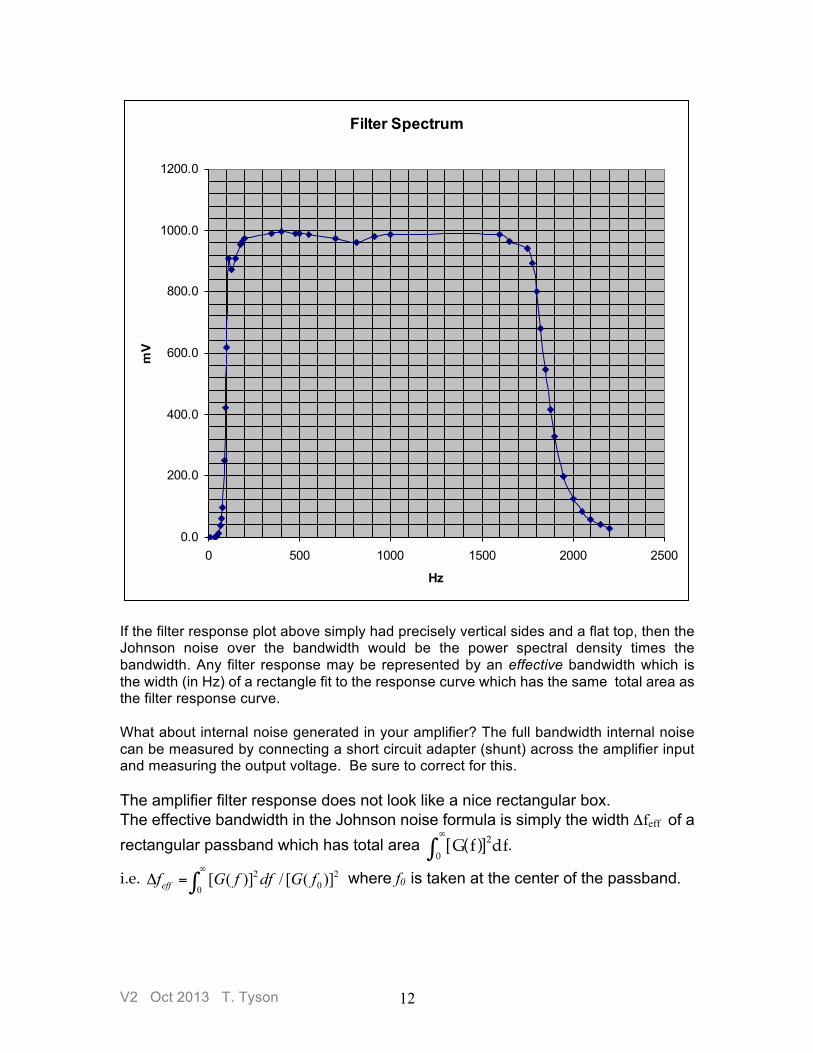
You can obtain the curve, or waveform, of the Amp/Filter by applying an input sine wave of known frequency and amplitude and then measuring the output voltage. Measuring the output at many frequencies across the band of interest and plotting the results on a frequency vs amplitude graph will provide results such as those on the next page. Note that this is just the filter in the amplifier box; you must also consider the filter caused by the input capacitance in parallel with the resistor (see above total noise spectrum plot.)

V2 Oct 2013 T. Tyson 12

If the filter response plot above simply had precisely vertical sides and a flat top, then the Johnson noise over the bandwidth would be the power spectral density times the bandwidth. Any filter response may be represented by an effective bandwidth which is the width (in Hz) of a rectangle fit to the response curve which has the same total area as the filter response curve. What about internal noise generated in your amplifier? The full bandwidth internal noise can be measured by connecting a short circuit adapter (shunt) across the amplifier input and measuring the output voltage. Be sure to correct for this. The amplifier filter response does not look like a nice rectangular box. The effective bandwidth in the Johnson noise formula is simply the width Δfeff of a rectangular passband which has total area [G(f)]2

0

∞

∫ df.

i.e. 2 200

[ ( )] / [ ( )]efff G f df G f∞

Δ = ∫ where f0 is taken at the center of the passband.

Filter Spectrum

0.0

200.0

400.0

600.0

800.0

1000.0

1200.0

0 500 1000 1500 2000 2500

Hz

mV

V2 Oct 2013 T. Tyson 13

The attenuator as well as the Picoscope use "dB power" (20 dB = factor of 100 in power, i.e. a factor of 10 in voltage). But do not trust their calibration. You must calibrate them yourself. The most accurate voltage standard you have is the Agilent digital rms voltmeter. Use it to calibrate the attenuator in the range you use it. When you do this, be sure to measure the input voltage to the attenuator while the oscillator is hooked into it (the oscillator's output voltage is loaded down by the attenuator's input resistance), and then measure the output voltage from the attenuator in the attenuation range you will use it. You will have to adjust the oscillator output voltage to stay at the same input voltage to the attenuator for different attenuation settings. You can also use the Agilent digital voltmeter to calibrate the picoscope dB power scale on its FFT spectrum. Most importantly, use the Agilent to make all voltage measurements directly, including rms noise voltage from the low noise bandpass amplifier. Use the Picoscope to visualize the spectrum and to make appropriate corrections to the rms voltage measured by the Agilent. You will find that you need to do this correction only in two cases: very high resistance (because of the change in gain profile which you see on the Picoscope spectrum), and at liquid nitrogen temperature (because of microphonic extra power in acoustic resonances which show nicely on your Picoscope spectrum). You should plot mean square voltage vs resistance at constant temperature, and mean square voltage vs temperature at constant resistance. You need this to derive Boltzmann's constant. TEMPERATURE DEPENDENCE OF THE JOHNSON NOISE [undertake this only if you are doing this plus 1/f and shot noise as part of your main PHY 123/253 project] A resistor in a glass thermal probe tube is provided to explore the temperature dependence of Johnson noise. Make sure that the interior of the tube is filled with helium or nitrogen gas to prevent condensation. Connect this probe directly to the INPUT connector on the amplifier (additional cable will only add capacitance and microphonic noise). In fact, calculate what a little capacitance like 10pF might do to the shape of your noise spectrum! You may want to consider this in your data analysis. Record the RMS voltage produced by this resistor at room temperature (~ 300 K as measured with thermometer), and at liquid nitrogen (77 K) and liquid helium (4.2 K). Also, use dry-ice for another temperature point. For low

V2 Oct 2013 T. Tyson 14

temperature measurements, make sure that the probe is filled with helium gas before it is immersed in the containers of liquid nitrogen and liquid helium. The helium gas will not become liquefied, and will help cool the resistor to the final temperature by conducting the heat away from it. Plot the rms noise voltage as a function of the temperature. Also, measure the resistance of the resistor at each of the temperatures (since the resistance of most resistors is a strong function of the temperature!). If you find any discrepancy between the measurement and the theory, suggest what their source(s) might be.

Measurements of noise are very important to physics experiments, because the actual noise levels in the experiment can determine whether one can measure small signal levels in the experiment. Measurements of noise power spectra as described here are frequently performed to understand the sources of the noise in the experiment. If you understand the noise in your experiment, you can then work to reduce noise sources by, for example, choosing components with less noise, averaging longer to reduce the effects of noise on the signal, or working in frequency regions where the noise is lower. In fact, specialized frequency analyzers exist; these are instruments which can easily measure such noise spectra (see below for an example: the PicoScope.) Some modern digital sampling oscilloscopes have a useful FFT option, and can be used to explore a wide frequency spectrum. Not only are there other sources of noise, there are also other sources of interference which may introduce systematic errors. For example, the local FM station has a particularly strong signal in the lab (you should look for this and be sure it is not present at the low-level parts of your circuit by probing with a scope or spectrum analyzer. Even if your scope does not have a FFT option you can change the time base and sensitivity to see this sine wave if it is present.) This noise power spectrum measurement by a computer and fast Fourier Transform (PicoScope) is particularly useful for measuring the noise of the resistor in the separate probe as a function of temperature (room temperature (~300K), in crushed dry ice (195K), and in liquid nitrogen (77K). The noise from

V2 Oct 2013 T. Tyson 15

this resistor is particularly susceptible to microphonic noise. Microphonic noise is the noise voltage generated in electric wires due to their motion through capacitive effect or piezo-electric effect. Thus it can be generated from the probe being shaken, by people walking in the room causing vibrations in the probe, etc. Measuring the noise power spectrum allows you to distinguish the Johnson noise (which is not frequency dependent) from microphonic noise, as well as electrical pickup from the AC power line frequency (60Hz) and noise from plasma discharges (lights!) that peak at specific frequencies such as multiples of 60Hz.

REFERENCES

• Reif, Fundamentals of Statistical and Thermal Physics, pp. 589 - 594 • Kittel, Thermal Physics, pp. 98-102 • Kittel, Elementary Statistical Physics, pp. 141-149. • Nyquist, Phys. Rev. 32, 110 (1928)