Joint meeting of The British, Portuguese and Spanish Sections of the

Combustion Institute

12-13 April 2016 Fitzwilliam College

Cambridge UK

Contents

Programme 1

Invited Lecture 3

Extended Abstracts

Sprays and Droplets 8

DNS of Turbulent Flames 1 14

Fuels 20

DNS of Turbulent Flames 2 31

Chemical Kinetics and Soot 41

DNS of Turbulent Flames 3 49

Diagnostics 57

Laminar and Turbulent Flames 1 64

Biomass Combustion 70

Laminar and Turbulent Flames 2 75

Flames and Auto-ignition 80

Laminar and Turbulent Flames 3 86

Flames, Droplets and Particles 92

Combustion Instability 100

ALL PLENARIES AT REDDAWAY ROOM

ALL TALKS IN THIS COLUMN AT TRUST ROOM ALL TALKS IN THIS COLUMN AT REDDAWAY ROOM

LUNCH AT UPPER HALL

DINNER AT MAIN HALL

Time09:30-10:0010:00-10:15

10:15-11:10

11:10-11:30Sprays and Droplets DNS of Turbulent Flames 1

11:30 S. Gallot Lavallée, W. P. Jones, F. Biagioli, B. Bunkute, K.J. Syed

11:30 N. A. K. Doan, N. Swaminathan and Y. Minamoto

Stochastic Fields Method Applied To Turbulent Swirling Flames With Acoustic Perturbations

DNS of partially premixed MILD combustion: Preliminary investigation

11:30-12:30 11:50 C. Nicoli, B. Denet 11:50 Cesar Dopazo, Luis Cifuentes and Jesus MartinRich spray flame speed Enstrophies normal and tangential to non-material iso-scalar

surfaces 12:10 J. M. Tejera and F. J. Higuera 12:10 Tomas B. Matheson and Edward S. Richardson

Vaporization and combustion of a spray of electrically charged droplets of heptane in a preheated gas

Mixture fraction-progress variable dependence in partially-premixed flames

12:30-14:00Fuels DNS of Turbulent Flames 2

14:00 B S. Soriano, T, B. Matheson, E S. Richardson 14:00 Jiawei Lai, Nilanjan Chakraborty, Markus KleinEffects of residence time on flame speed in autoignitive mixtures of methane and n-heptane

Assessment of algebraic Flame Surface Density closures in the context of Large Eddy Simulations for head-on quenching of turbulent premixed flames with non-unity Lewis number

14:20 Carlos Herce, Javier Pallarés, Carmen Bartolomé, Cristóbal Cortés

14:20 Y. X, Yang, K.K.J. Ranga Dinesh

Thermal Vaporization Of Sub-Bituminous Waste Coal In A 160mwe Utility Boiler: A CFD Analysis

Investigation of Flame-Wall Interaction with Rough-Wall: A DNS Study

14:00-15:40 14:40 David Lázaro, Mariano Lázaro, Daniel Alvear 14:40 Cesar Dopazo, Jesus Martin and Luis Cifuentes Thermal degradation effects of the atmosphere and lid used in STA test for thermoplastic polymers

Rotation of non-material iso-scalar surfaces

15:00 Alonso, A.; Lázaro, D; Lázaro, M.; Alvear, D. 15:00 Edward S. Richardsona, Jacqueline H. ChenMaterial pyrolysis estimation combining mass and energy as optimization targets

Analysis of Turbulent Flame Propagation in Equivalence Ratio-Stratified Flow

15:20 Xi Zhuo Jiang, Xujiang Wang, Kai H. Luo 15:20 U Ahmed, M Zimon, G Nivarti, R Prosser, R S CantReactive Force Field Molecular Dynamics Study on Hydrothermal Oxidation and Hydrolysis of Ethanol at Supercritical Conditions

Influence of pressure Hessian on flame turbulence interaction in premixed combustion

15:40_16:00Chemical Kinetics and Soot DNS of Turbulent Flames 3

16:00 Qian Mao, Adri C.T. van Duin, K. H. Luo 16:00 Luis Cifuentes, Nilanjan Chakraborty, Cesar DopazoFormation of Nascent Soot Clusters from Polycyclic Aromatic Hydrocarbons: A ReaxFF Molecular Dynamics Study

Kinetic energy and its dissipation rate budgets in statistically planar turbulent premixed flames at different Lewis numbers

16:20 F. Viteria, M. Abiána, Á. Millera, R. Bilbao, M.U. Alzueta 16:20 A J AspenEffect of the SO2 and H2S presence on the formation of PAH and soot during the pyrolysis of ethylene

Effects In Turbulent Premixed Flames

16:00-17:20 16:40 P. Koniavitis, W. P. Jones, S. Rigopoulos 16:40 Dong-hyuk Shin, Edward S RichardsonA methodology for selecting constrained species in RCCE via CSP

Self-similarity of Turbulent Unsteady Jet

17:00 Fabian Sewerin, Stelios Rigopoulos 17:00 Nadeem A. Malik An LES-detailed PBE model with PBE-grid adaptivity for predicting soot formation in a turbulent diffusion flame

Implicit DNS of Numerical Combustion with Detailed Chemistry

19:00 Reception at Upper Hall19:30 Conference Banquet at Main Hall

Bar open until 11.30pm

Joint meeting of the British, Portuguese and Spanish Sections of the Combustion Institute

Break

Tuesday, 12 AprilActivities

Registration & Refreshment Welcome

Invited lectureAmable Liñán

The flameless reacting mode of combustion and the explosion limits of gaseous mixtures in spherical vessels.

Break

Lunch

Cambridge, UK, 12-13 April, 2016

1

Time

09:30 Alvaro Sobrino, Ennio Luciano, Javier Ballester 09:30 D. Mira, S. Gövert, J.B.W. Kok2, M. Vázquez, G. HouzeauxRobust automatic control of a laboratory lean premixed combustor based on flame signals

Numerical simulations of turbulent combustion applications using the parallel multiphysics code Alya

9:30-10:30 09:50 Nelson Alves, Teodoro P. Trindade, Edgar C. Fernandes 09:50 Huangwei Zhang, Epaminondas Mastorakos

Spectral identity of gas fuels: temperature effect LES/CMC Modelling of Swirl Flames in A Gas Turbine Model Combustor with Dual Swirlers

010:10 L. Fan, Y. Gao, A. Hayakawa and S. Hochgreb 10:10 Maqsood Alam, Jennifer Wen, Siaka Dembele Simultaneous 2D gas-phase temperature and velocity measurements by thermographic particle image velocimetry with ZnO tracers

Numerical Modelling of Liquid Pool Fires to Predict Burning Rate with a CFD Approach

10:30-10:35

10:35:11:30

11:30-11:50

11:50 Ibarra, G. Aragon, D. Sanz, E. Rojas, I. Gómez, J. J. Rodríguez-Maroto, C. Gutierrez-Canas

11:50 Carlos Montañés, Norberto Fueyo, Ramón Chordá, Eduardo Gimeno

11:50-12:30On the limits of current predictive tools for an efficient control of trace emissions from agricultural waste combustion

Flamelet Generated Manifolds for industrial flows: problems and extensions

12:10 Jun Li, Manosh C Paul, Krzysztof M. Czajka 12:10 G. Garcia-Soriano, S. Margenat, F.J. Higuera, J.L. Castillo, P.L. Garcia-Ybarra

Ignition behaviour of biomass particles in a down-fire reactor for optimization of co-firing performance

Laminar jet flames of methane–air mixtures under strong curvatures

12:30-14:00

14:00 João P. Marcelino, João M. Pires, Edgar C. Fenrandes 14:00 Xujiang Wang, Xi Zhuo Jiang, K. H. LuoInfluence of Rich-Lean Interactions on the Flame Topology Structures of Lean Premixed Turbulent H2/Air Flames at High

Karlovitz Numbers 14:20 Nabil Meah, Edward S. Richardson 14:20 Sergio Margenat, Gabriel Garcia-Soriano, Jose L. Castillo and

Pedro L. Garcia-Ybarra

14:00-15:00 Double Conditional Moment Closure simulation of n-heptane spray autoignition

Methane–air laminar jet flames in high-pressure combustion

14:40 Magin Lapuerta, Juan José Hernandez, David Fernández-Rodríguez, Alexis Cova

14:40 G. V. Nivarti and R. S. Cant

Autoignition of blends butanol-ethanol with diesel and biodiesel fuels in a constant-volume combustion chamber

Influence of Flame Surface on the Bending Effect in Turbulent Premixed Flames

15:00-15:20

15:20 S P. Malkeson, D Wacks, Lizhong Yi, N Chakraborty 15:20 Yu Xia, A. S. Morgans, W. P. Jones, G.BulatAnalysis of the co-variance of fuel mass fraction and mixture fraction in turbulent flame-droplet interaction: A Direct Numerical Simulation study

Combining low order network modelling with incompressible ame LES for thermoacoustic instability in an industrial gas turbine combustor

15:20-16:40 15:40 P.E. Mason, L.I. Darvell, J.M. Jones, A. Williams 15:40 N. Treleaven, J. Su, A. Garmory, G. PageFlame-Combustion Studies On Single Particles Of Solid Biomass

Modelling the Acoustic Response of Fuel Sprays in Gas Turbines

16:10 D. Fernández-Galisteo, C. Jiménez, M. Sánchez-Sanz, V.N. Kurdyumov

16:10 Duran, Y. Xia, A. S. Morgans, X. Han

Effects of stoichiometry on premixed flames propagating in planar microchannels

Dispersion of entropy waves advecting through combustion chambers

16:30 Jacob W. Martin, Peter Grančiča, Dongping Chen, Sebastian Mosbacha, Markus KraftDynamic gas interactions with polycyclic aromatic hydrocarbon clusters

Flames and Autoignition Laminar and Turbulent Flames 3

Diagnostics Laminar and Turbulent Flames 1

Break

Lunch

Nilanjan ChakrabortyLewis number effects on turbulent premixed combustion and modelling implications: A Direct Numerical Simulation perspective.

Invited lecture

Closing

Break

ActivitiesWednesday 13 April 2016

Break

Biomass Combustion Laminar and Turbulent Flames 2

Flames, Droplets and Particles Combustion Instability

2

Invited Lectures

3

The flameless reacting mode of combustion, and the explosion

limits of gaseous mixtures in spherical vessels.

Amable LinanETSI Aeronauticos, Universidad Politecnica de Madrid, Spain

Immaculada IglesiasGrupo de Mecanica de Fluidos, Universidad Carlos III de Madrid, Spain

Daniel Moreno, Antonio L. Sanchez, Forman A. WilliamsDepartment of Mechanical and Aerospace Engineering, UCSD, USA

April 5, 2016

In this lecture, the basic concepts associated with the large-activation-energy techniques areintroduced beginning with a short analysis of the Semenov homogeneous thermal-explosion model.We then revisit Frank-Kamenetskii’s analysis of thermal explosions, using also a single-reactionmodel with an Arrhenius rate, having a large activation energy, to describe the transient combustionof initially cold gaseous mixtures enclosed in a spherical vessel with a constant wall temperature.The analysis shows two modes of combustion depending on the value of a Damkohler number,defined as the ratio of the characteristic heat-conduction time to the homogeneous thermal-explosiontime at the wall temperature. In the first mode of combustion, a flameless slowly reacting modefor low wall temperatures or small vessel sizes (i.e. small values of the Damkohler number), thetemperature rise due to the reaction is kept small by the heat-conduction losses to the wall, soas not to change significantly the order of magnitude of the reaction rate. In the second modeof combustion, for values of the Damkohler number above a critical value of order unity, theslow reaction rates occur only in the first ignition stage, which ends abruptly when very largereaction rates cause a temperature runaway, or thermal explosion, at a well-defined ignition timeand location, which triggers a flame that propagates across the vessel to consume rapidly thereactant. We define the explosion limits, in agreement with Frank-Kamenetskii’s analysis, by thelimiting conditions for existence of the slowly reacting mode of combustion. In this mode, a quasi-steady temperature distribution is established after a transient reaction stage with small reactantconsumption. Most of the reactant is burnt, with nearly uniform mass fraction, in a second longstage, when the temperature follows a quasi-steady balance between the rates of heat conductionto the wall and of chemical heat release.

The second part of this lecture will address the effect of buoyancy-driven motion on the quasi-steady “slowly reacting” mode of combustion and on its thermal-explosion limits. For gaseousmixtures under normal gravity, the critical Damkohler number increases through the effect ofbuoyancy-induced motion on the rate of heat conduction to the wall, measured by an appropriateRayleigh number Ra. In the present analysis, for small values of Ra, the temperature is given inthe first approximation by the spherically symmetric Frank-Kamenetskii solution, used to calculatethe accompanying gas motion, an axisymmetric annular vortex determined at leading order by thebalance between viscous and buoyancy forces, which we call the Frank-Kamenetskii vortex. Thisflow is used in the equation for conservation of energy to evaluate the influence of convection onexplosion limits for small Ra, resulting in predicted critical Damkohler numbers that are accurateup to values of Ra on the order of a few hundred.

4

Lewis number effects on turbulent premixed combustion and modelling im-plications: A Direct Numerical Simulation perspective

Nilanjan Chakraborty1 1School of Mechanical and System Engineering, Newcastle University, Claremont Road, Newcastle

Upon Tyne, NE1 7RU, UK Abstract Differential diffusion of heat and mass is often character-ised in terms of Lewis number 𝐿𝑒 (defined as the ratio of thermal diffusivity to mass diffusivity). Although every species in a combustion process has its own Lewis number, a characteristic Lewis number can be assigned to a given premixed combustion process in terms of the Lewis num-ber 𝐿𝑒 of the deficient species [1], by heat release measure-ments [2], or by a linear combination of the mole fractions of the mixture constituents [3]. A number of analyses demonstrated that the non-unity Lewis number has signifi-cant influence on the burning rate and wrinkling of laminar flames and is responsible for thermo-diffusive instability for 𝐿𝑒 < 1, (readers are referred to Refs. [4, 5] and the ref-erences therein for an extensive review in this regard). Ex-perimental investigations indicated that the effects of char-acteristic Lewis number do not disappear even for turbulent flames at high values of turbulent Reynolds number [3, 6]. These differential diffusion effects due to non-unity Lewis number play a key role in lean-hydrogen-air flames. This paper will review the physical understanding obtained from three-dimensional compressible Direct Numerical Simulation (DNS) data regarding differential diffusion rates of heat and mass arising from the non-unity Lewis number, and its modelling implications. It has been found that the rate of diffusion of fresh reactants into the reaction zone supersedes the rate at which heat is diffused out in the Le < 1.0 flames. This gives rise to the simultaneous pres-ence of high reactant concentration and high temperature, and thus the burning rate and flame area generation area are greater in the Le < 1.0 flames than in the unity Lewis number flames with similar turbulent flow conditions in the unburned reactants. Just the opposite mechanism gives rise to a reduced burning rate in the Le > 1.0 flames, in com-parison to the corresponding unity Lewis number flame.

The augmentation of burning rate with decreasing 𝐿𝑒 gives rise to a strengthening of flame normal acceleration and dilatation rate. This tendency is more prevalent in flames with Le << 1.0 due to thermo-diffusive instabilities. The Lewis number dependences of flame normal accelera-tion and dilatation rate have significant influences on tur-bulent kinetic energy and enstrophy transport through pres-sure dilatation and baroclinic terms respectively [7,8]. This leads to stronger flame-generated turbulence and enstrophy generation within the flame brush in the 𝐿𝑒 < 1 flames than in the unity Lewis number flame subjected to statisti-cally similar unburned gas turbulence, and this tendency

* Corresponding author: nilanjan.chakraborty@newcastle.ac.uk

strengthens with decreasing Lewis number [9]. Strengthen-ing of flame normal acceleration eventually leads to coun-ter-gradient transport of turbulent kinetic energy, reaction progress variable, and its variance and dissipation rate with Le << 1.0 under similar turbulent conditions on the un-burned gas side, for which gradient transport has been ob-served for flames with Le ≈ 1.0 [7, 9-11].

The global Lewis number also significantly affects the alignment of scalar gradient with local principal strain rates [12] through its influence on flame normal acceleration and dilatation rate. It has been found that reactive scalar gradi-ent shows increased tendency to align preferentially with the most extensive principal strain rate with decreasing Lewis number Le. This has been shown to have significant influences on the normal strain rate contribution to the Flame Surface Density (FSD) and Scalar Dissipation Rate (SDR) transport [10,13], and the normal strain rate contri-bution is found to dissipate FSD and SDR in flames with Le <<1 under similar turbulent conditions on the unburned gas side, for which scalar gradient is created by normal strain rate contribution in the FSD and SDR transport equa-tions for flames with Le ≈ 1.0. The increased heat release with decreasing Le leads to strengthening of dilatation rate and its contribution to the FSD and SDR transports. The contribution of dilatation rate on the FSD and SDR acts to generate FSD and SDR for all flames irrespective of Le but this effect strengthens with decreasing Le [10,13].

The differential diffusion of heat and mass has signifi-cant influences on the curvature dependences of tempera-ture and heat release rate in non-unity Lewis number flames [14,15], and this gives rise to a finite probability of finding super-adiabatic temperature even under globally-adiabatic conditions. These super-adiabatic hot spots in the Le <<1 cases play an important role in increasing the wall heat flux and quenching distance for head-on quenching of turbulent premixed flames [16]. Furthermore, the afore-mentioned curvature dependence of chemical reaction rate affects the local stretch rate dependence of flame displace-ment speed Sd [14,15]. The combined reaction and normal diffusion components of displacement speed (i.e. (Sr +Sn)) and the magnitude of the reaction progress variable gradi-ent become increasingly positively (negatively) correlated with local curvature with decreasing (increasing) Lewis number for flames with Le < 1 (Le >1).This, in turn, affects the statistical behaviours of the curvature and propagation terms of the FSD and SDR transport equation.

Detailed explanations for the aforementioned differen-tial diffusion effects induced by non-unity Lewis number

5

will be provided and discussed in depth in this paper. The implications of these physical mechanisms for turbulent scalar flux, FSD and SDR based closures [9-13] in the con-text of Reynolds Averaged Navier Stokes (RANS) and Large Eddy Simulations (LES) will be discussed based on a-priori analysis of DNS data.

Acknowledgements The author is grateful to EPSRC and N8/ARCHER for

the financial and computational support respectively. References [1] Mizomoto, M., Asaka, S., Ikai, S. and Law, C.K. (1984), Effects of preferential diffusion on the burning in-tensity of curved flames, Proc. Combust. Inst., Vol. 20, 1933-1940. [2] Law, C.K., Kwon, O.C. (2004) Effects of hydrocarbon substitution on atmospheric hydrogen–air flame propaga-tion, Int. J. Hydrogen Energy, Vol. 29, pp. 867-879. [3] Dinkelacker, F., Manickam, B., Mupppala, (2011), Modelling and simulation of lean premixed turbulent me-thane/hydrogen/air flames with an effective Lewis number approach, Combust. Flame, Vol. 158, pp. 1742-1749. [4] Sivashinsky, G.I., (1983), Instabilities, pattern for-mation and turbulence in flames, Ann. Rev. Fluid Mech., 15,179-199. [5] Lipatnikov, A.N., Chomiak, J. (2005) Molecular transport effects on turbulent flame propagation and struc-ture”, Prog. Energy Combust. Sci., 31, 1-73. [6] Abdel-Gayed, R.G., Bradley, D., Hamid, M., and Lawes, M., (1984), Lewis number effects on turbulent burning velocity, Proc. Combust. Inst., 20,505-512. [7] Chakraborty, N., Katragadda, M., Cant, R.S. (2011) Ef-fects of Lewis number on turbulent kinetic energy transport in turbulent premixed combustion, Phys. Fluids, 23, 075109. [8] Chakraborty, N., Konstantinou, I., Lipatnikov, A. (2016) Effects of Lewis number on vorticity and enstrophy transport in turbulent premixed flames, Phys. Fluids, 28, 015109. [9] Chakraborty, N., Cant, R.S. (2009) Effects of Lewis number on scalar transport in turbulent premixed flames, Phys. Fluids, 21, 035110. [10] Chakraborty, N., Swaminathan, N. (2010) Effects of Lewis number on scalar dissipation transport and its mod-elling implications for turbulent premixed combustion, Combust. Sci. Technol.182, 1201-1240. [11] Chakraborty, N., Swaminathan, N. (2011) Effects of Lewis number on scalar variance transport in turbulent pre-mixed flames, Flow Turb. Combust. , 87, 261-292. [12] Chakraborty, N., Klein, M., Swaminathan, N. (2009) Effects of Lewis number on reactive scalar gradient align-ment with local strain rate in turbulent premixed flames, Proc. Combust. Inst., 32, 1409-1417. [13] Chakraborty, N., Cant, R.S. (2011) Effects of Lewis number on Flame Surface Density transport in turbulent premixed combustion, Combust. Flame, 158, 1768-1787. [14] Chakraborty, N., Cant, R.S. (2005) Influence of Lewis number on curvature effects in turbulent premixed flame propagation in the thin reaction zones regime, Phys. Fluids, 17,105105.

[15] Chakraborty, N., Klein, M. (2008) Influence of Lewis number on the Surface Density Function transport in the thin reaction zones regime for turbulent premixed flames.” Phys. Fluids, 20, 065102. [16] Lai, J., Chakraborty, N. (2015) Effects of Lewis Number on Head on Quenching of Turbulent Premixed Flame: A Direct Numerical Simulation analysis, Flow Turb. Combust., DOI 10.1007/s10494-015-9629-x.

𝐿𝑒 = 0.34

𝐿𝑒 = 0.60

𝐿𝑒 = 0.8

𝐿𝑒 = 1.00

𝐿𝑒 = 1.20

Fig.1: Distribution of normalised vorticity magni-tude (𝝎𝒊𝝎𝒊)𝟏/𝟐 × 𝜹𝒕𝒉 𝑺𝑳⁄ in the central 𝒙𝟏 − 𝒙𝟑 plane at time 𝒕 = 𝒕𝒄𝒉𝒆𝒎 for cases with initial values of nor-malized root-mean-square turbulent velocity fluctu-ation 𝒖′ 𝑺𝑳⁄ = 𝟕. 𝟓 and integral length scale to flame thickness ratio 𝒍 𝜹𝒕𝒉⁄ = 𝟐. 𝟓 with 𝑺𝑳 and 𝜹𝒕𝒉 being unstrained laminar burning velocity and flame thickness respectively. White lines show reaction progress variable contours from c=0.1 to 0.9 (from left to right) in steps of 0.1.

6

Extended Abstracts

7

STOCHASTIC FIELDS METHOD APPLIED TO TURBULENT SWIRLINGFLAMES WITH ACOUSTIC PERTURBATIONS

S. Gallot Lavallee⇤, W. P. JonesMechanical Engineering Department, Imperial College London, SW7 2AZ UK

F. Biagioli, B. Bunkute, K.J. SyedGeneral Electrics Power, 7 Brown Boveri Strasse, Baden, 5401, CH

⇤E-mail: simon.gallot-lavallee@imperial.ac.uk

1 Introduction

The dynamic response to acoustic perturbation of devices operating in the lean premixed combustion regime canhave severe consequences on the combustor integrity and there is thus a clear need for an improved understandingof the phenomenon. In this work Large Eddy Simulation (LES) is applied in conjunction with the sgs pdf equationapproach with the solution of the corresponding equation being obtained with the stochastic fields method, [1]. Thegeometry and boundary conditions implemented are representative of the General Electrics Conical Burner (seeFigure 1), which comprises two sections, a mixing section where the mixing between fuel and air occurs and thecombustor where the flame stabilises. The fuel is methane. The complexity of the mixing section is such that theuse of an unstructured CFD code is the optimum approach to simulation in this section. On the other hand thecombustor is simpler in terms of geometry and can thus be simulated using the block structured combustion LEScode BOFFIN-LES. The characterisation of the mixing section is obtained by calculating the unit response of thesystem by means of the Wiener-Hopf filtering technique in conjunction with a Proper Orthogonal Decomposition(POD) of the velocity components and mixture fraction. Once the turbulent and dynamic behavior of the mixingsection is obtained the velocity field, mixture fraction and temperature can be obtained by reverse transformation ofthe convolution between the characteristic function and the forcing signal applied at the inlet of the mixing section[2]. Having the ability of obtaining the dynamic response of a system without the need of performing a full CFDcalculation allows the coupling with the LES-pdf code BOFFIN-LES responsible for the combustion simulations.Once the flame is simulated, it is possible to relate the heat release rate of the flame to the inlet perturbation throughthe introduction of a Flame Transfer Function (FTC).

2 Mathematical Modelling

Reactive flows are fully described by the conservation equations for mass, momentum and the scalars quantities ofinterest. In the present context these comprise the species mass fraction and the mixture enthalpy. Because of spacelimitations no further details of the equations governing mass and momentum conservation will be provide here. Forthe present case the conservation equations for the species mass fractions and enthalpy can be written in the generalform:

@⇢ge�↵

@t

+@⇢g

e�↵euj@xj

=@

@xj

µ

�

@

e�↵

@xj

!+@J sgs

j

@xj+ ⇢g!↵

��

�(1)

where �↵ is the ↵th scalar field, and where � is a constant Prandtl or Schmidt number as appropriate. The filteredform of the conservation equations for specific molar mass of the chemical species contain the filtered net formationrates of the chemical species through chemical reaction. The direct evaluation of these poses serious difficulties andto overcome this a joint sgs-pdf evolution equation formulation is adopted. The equation describing the evolution ofthe pdf, is solved using the Eulerian stochastic field method. The sub grid scale filtered pdf Psgs( ) is representedby an ensemble of Ns stochastic fields for each of the N scalars namely ⇠n↵(x, t) with 1 n Ns, 1 ↵ N . Inthe present work the Ito formulation of the stochastic integral is adopted, the stochastic fields evolve according to:

⇢d⇠n↵ =� ⇢ui@⇠

n↵

@xidt+

@

@xi

�0@⇠

n↵

@xi

�dt+ ⇢

s2�0

⇢

@⇠

n↵

@xjdWn

i � ⇢

2⌧sgs

⇣⇠

n↵ � e�↵

⌘dt+ ⇢!

n↵(⇠

n)dt (2)

where �0 represents the total diffusion coefficient and dW

ni represent increments of a (vector) Wiener process,

different for each field but independent of the spatial location x. This stochastic term has no influence on the first

1

8

(a) Mixing Section. (b) Combustor.

Figure 1: Mesh of the mixing section and combustor.

(a) LES configuration A. (b) Experiment configuration A.

(c) LES configuration B. (d) Experiment configuration B.

Figure 2: Contour plots of velocity components for different configurations normalised with the bulk velocity.

moments (or mean values) of ⇠n↵. The stochastic fields given by (2) form an equivalent stochastic system (both setshave the same one-point pdf, [3]) smooth on the scale of the filter width. The results of the CFD calculation are usedin order to obtain the FTF (X) which is defined by the ratio of the perturbation in the mass flow rate at the inlet ofthe system and its response in terms of heat release.

3 Results and Comnclusions

To evaluate the results of the CFD simulation in the burner and the combustor these are compared with experimentaldata obtained by PIV measurements. Two different configuration are considered corresponding to two different bulkvelocities. A comparison of the simulated and experimental velocities in the burner, both normalised with the bulkvelocity respectively are presented in Figure 2 for both configurations A and B. The simulation appears to be in goodagreement with the experiments with the recirculation zone being accurately represented and the magnitude of thevelocity well captured. The profiles to be imposed as boundary conditions for the LES-pdf simulations are consistentwith the perturbation imposed at the inlet.

References

[1] S. Gallot-Lavallee and W. Jones, “Large eddy simulation of spray auto-ignition under egr conditions,” Flow, Turbulenceand Combustion, vol. 96, no. 2, pp. 513–534, 2016.

[2] G. Borghesi, F. Biagioli, and B. Schuermans, “Dynamic response of turbulent swirling flames to acoustic perturbations,”Combustion Theory and Modelling, vol. 13, no. 3, pp. 487–512, 2009.

[3] C. W. Gardiner, Handbook of Stochastic Methods. For Physics, Chemistry and the Natural Science, vol. 13 of SpringerSeries Synergetics. Springer, 1983.

2

9

!!Joint!British,!Spanish!and!Portuguese!Section!Combustion!Meeting!9!!12913th!April!2016!!9!!Cambridge!UK!!!

Rich spray flame speed

C. Nicoli1, B. Denet2*

1 M2P2 , Aix-Marseille Université/ CNRS/ Centrale Marseille , UMR 7340, 13451 Marseille France,

2 * IRPHE, Aix-Marseille Université/ CNRS/ Centrale Marseille, UMR 7342, 13384 Marseille France

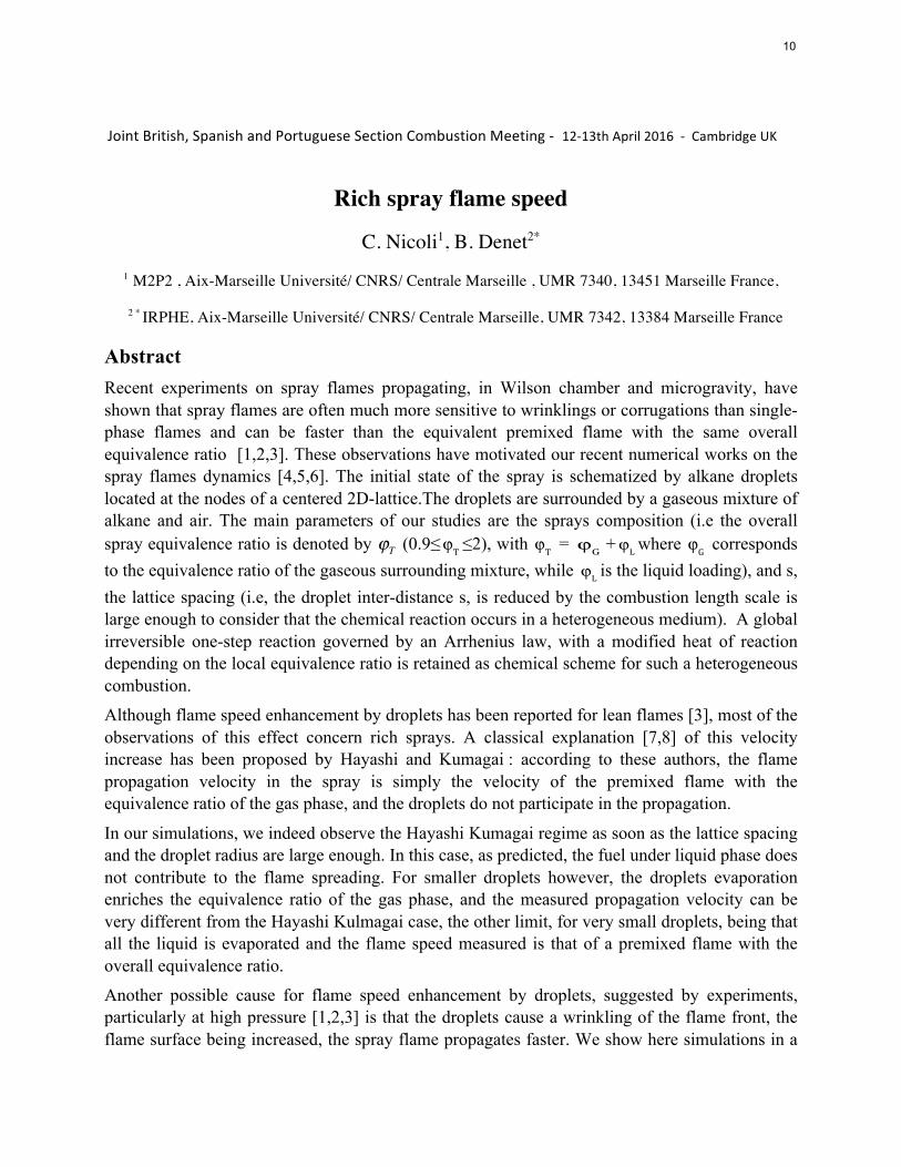
Abstract Recent experiments on spray flames propagating, in Wilson chamber and microgravity, have shown that spray flames are often much more sensitive to wrinklings or corrugations than single-phase flames and can be faster than the equivalent premixed flame with the same overall equivalence ratio [1,2,3]. These observations have motivated our recent numerical works on the spray flames dynamics [4,5,6]. The initial state of the spray is schematized by alkane droplets located at the nodes of a centered 2D-lattice.The droplets are surrounded by a gaseous mixture of alkane and air. The main parameters of our studies are the sprays composition (i.e the overall spray equivalence ratio is denoted by ϕT (0.9≤!ϕT ≤2), with !ϕT = !ϕG +!ϕL where !ϕG corresponds to the equivalence ratio of the gaseous surrounding mixture, while !ϕL is the liquid loading), and s, the lattice spacing (i.e, the droplet inter-distance s, is reduced by the combustion length scale is large enough to consider that the chemical reaction occurs in a heterogeneous medium). A global irreversible one-step reaction governed by an Arrhenius law, with a modified heat of reaction depending on the local equivalence ratio is retained as chemical scheme for such a heterogeneous combustion.

Although flame speed enhancement by droplets has been reported for lean flames [3], most of the observations of this effect concern rich sprays. A classical explanation [7,8] of this velocity increase has been proposed by Hayashi and Kumagai : according to these authors, the flame propagation velocity in the spray is simply the velocity of the premixed flame with the equivalence ratio of the gas phase, and the droplets do not participate in the propagation.

In our simulations, we indeed observe the Hayashi Kumagai regime as soon as the lattice spacing and the droplet radius are large enough. In this case, as predicted, the fuel under liquid phase does not contribute to the flame spreading. For smaller droplets however, the droplets evaporation enriches the equivalence ratio of the gas phase, and the measured propagation velocity can be very different from the Hayashi Kulmagai case, the other limit, for very small droplets, being that all the liquid is evaporated and the flame speed measured is that of a premixed flame with the overall equivalence ratio.

Another possible cause for flame speed enhancement by droplets, suggested by experiments, particularly at high pressure [1,2,3] is that the droplets cause a wrinkling of the flame front, the flame surface being increased, the spray flame propagates faster. We show here simulations in a

10

larger domain where droplets trigger instabilities of the flame front (in this model hydrodynamic instability).

Funding : this study was funded by a support of the Research Program " Micropesanteur Fondamentale et Appliquee " - GDR 2799 - CNRS/CNES under the contract CNES/140569.!

References [1] D. Bradley, M. Lawes, S. Liao, A. Saat, Laminar mass burning and entrainment velocities and flame instabilities of isooctane, ethanol and hydrous ethanol/air aerosols, Combust. and Flame 161(6) (2014) 1620-1632.

[2] R. Thimothee, C. Chauveau, F. Halter, I. Gokalp, Rich spray flame propagating through a 2d-lattice of alkane droplets in air, Proceedings of ASME16 Turbo Expo 2015: Turbine Technical Conference and Exposition GT2015, 2015.

[3] H. Nomura, I. Kawasumi, Y. Ujiie, J. Sato, Effects of pressure on propagation in a premixture containing fine fuel droplets, Proc. Combust. Inst. 31 (2007) 2133-2140.

[4] C. Nicoli, B. Denet, P. Haldenwang., Lean flame dynamics through a 2d lattice of alkane droplets in air, Combust. Sci. and Tech. 186(2) (2014) 103-119.

[5] C. Nicoli, B. Denet, P. Haldenwang, Rich spray flame propagating through a 2d-lattice of alkane droplets in air, Combust. and Flame 4598-4611 . doi.org/10.1016/j.combustflame.2015.09.018

[6] C. Nicoli, B. Denet, P. Haldenwang, Spray flame dynamics in a rich droplet array, Flow Turbulence Combust. in press (2015) DOI 10.1007/s10494-015- 9675-4. [7] S. Hayashi, S. Kumagai, and T. SakaiFlame Propagation in Fuel Droplet-Vapor-Air Mixtures, . Proc Combust Institute., 15,445-451 1975 ! [8] S. Hayashi, S. Kumagai, and T. Sakai. Propagation velocity and structure of flames in droplet vapor air mixtures. Combust. Sci. and Tech., 15:169–177, 1976. !

!

11

Vaporization and combustion of a spray of electrically charged

droplets of heptane in a preheated gas

J. M. Tejera and F. J. Higuera

ETSIAE, Universidad Politecnica de Madrid,

Plaza Cardenal Cisneros 3, 28040 Madrid, Spain

A model is formulated of the vaporization and gas-phase combustion of a dilute spray ofelectrically charged droplets of heptane in a coflow of preheated air within a miniaturecombustion chamber, a configuration similar to some of the mesoscale catalytic systemswith heat recuperation proposed and tested by Gomez and coworkers [1, 2, 3, 4].

The mean distance between droplets is large compared to the initial radius of a dropletand small compared to the size of the spray. In these conditions, an Eulerian, mesoscaledescription of the gas flow [5] combined with a Lagrangian, particle-in-cell description ofthe droplets [6] can be used.

The droplets interact mainly through the surrounding gas and through the electricfield induced by the electric charges they carry. Direct interactions between droplets arerare events that can be neglected. Mass, momentum and energy equations are writtenfor each droplet which contain the force exerted by the gas on the droplet, the heatflux reaching the droplet by conduction from the gas, and the droplet vaporization rate.These magnitudes depend on the local conditions of the gas seen by the droplet and on theradius, velocity and temperature of the droplet. Approximations valid for small values ofthe Reynolds numbers of the slip and vaporization Stefan flows, and for large values of theratio of the latent heat to the thermal energy of the liquid, are used. Coulomb explosionswhereby a droplet loses a fraction of its electric charge occur when vaporization drivesthe droplet to the Rayleigh limit, and generate a population of charged nanometer-sizeresidues that drift relative to the gas at a velocity proportional to the electric field untilthey reach the walls of the chamber. A method of particles is used in which each particlerepresents a parcel of the one-droplet phase space containing a large number of droplets.

Mass, momentum and energy conservation equations are written for the gas in ele-mentary control volumes of size large compared to the mean distance between dropletsbut small compared to the size of the system. These volumes enclose many droplets ex-changing mass, momentum and energy with the gas, whose e↵ect appears as distributedsource terms in the gas equations. Combustion in the gas phase is modelled by a sin-gle irreversible reaction with a rate given by an Arrhenius law with activation energyand frequency factor chosen to reproduce ignition delay times measured by Ciezki andAdomeit [7] in shock tube experiments.

A single electrospray source is considered that injects small droplets of heptane witha coflow of preheated air through a circular orifice at one of the bases of a cylindricalchamber. Axial symmetry conditions are imposed at a certain distance from the axis ofthe orifice to approximately model the two-dimensional arrays of sources used by Kyritsiset al. [1] and Deng et al. [3].

The e↵ects of the inlet gas temperature (T1), the fuel flow rate (Q) and the overall

12

1

2

3

4

5

6

1.2 1.6 2 2.4

Tm/T

0

T1/T0

0 13

2

Figure 1: Mixing temperature, Tm =R⇢vT d�/

R⇢u d�, at the outlet of the chamber as a function of the

inlet gas temperature T1, both scaled with the inlet droplet temperature T0 = 293 K, for Q = 1.50 ml/h,� = 0.7 (0); Q = 1.50 ml/h, � = 0.35 (1); Q = 2.54 ml/h, � = 0.35 (2); and Q = 3.38 ml/h, � = 0.35(3). Here ⇢, T and v are the density, temperature and axial velocity of the gas, and the integrals extendto the cross-section of the chamber.

equivalence ratio (�) are analyzed. The outlet mixing temperature as a function of theinlet gas temperature features frozen and intense combustion branches, with ignition andextinction values of T1 that depend on Q and �; see Fig. 1.

Two di↵erent combustion modes have been found for globally lean systems. In oneof these modes mode, combustion begins immediately upon fuel vaporization, in a layerof intense reaction that locally depletes the oxygen and leaves behind a region of hightemperature fuel vapor surrounded by a di↵usion flame. In the other mode, combustionoccurs in a lean premixed flame located well above the spray, where the fuel has fullyvaporized and mixed with the air. The first combustion mode depends on rapid vapor-ization of the fuel to generate a region of excess fuel vapor. The distance of the intensereaction layer to the injection orifice increases with the flow rate of fuel (which also in-creases the size of the droplets for the atomizer considered) until transition to the secondcombustion mode occurs at a certain value of this parameter. This transition can becontrolled acting on the electric charge of the droplets, which determines the divergenceof the spray and thus the maximum fuel vapor concentration, or on the radius of theinjection orifice, which determines the inlet velocity of the gas for given values of Q and�. Transition between the two modes is discussed, and ignition and extinction conditionsare determined.

Acknowledgments. This work was supported through the Spanish MINECO projectsCSD2010-00011 and DPI2013-47372-C02-02.

[1] D. C. Kyritsis, I. Guerrero-Arias, S. Roychoudhury, A. Gomez, Proc. Combust. Inst. 29, 965 (2002).[2] D. C. Kyritsis, B. Coriton, F. Faure, S. Roychoudhury, A. Gomez, Combust. Flame 139, 77 (2004).[3] W. Deng, J. F. Klemic, X. Li, M. A. Reed, A. Gomez, Proc. Combust. Inst. 31, 2239 (2007).[4] A. Gomez, J. J. Berry, S. Roychoudhury, B. Coriton, J. Huth, Proc. Combust. Inst. 31, 3251 (2007).[5] F. A. Williams, Combustion Theory, 2nd ed., Benjamin Cummings, Menlo Park, CA, 1985.[6] C. K. Birdsall, A. B. Langdon, Plasma Physics Via Computer Simulation, Taylor & Francis, New

York, 1991.[7] H. K. Ciezki, G. Adomeit, Combust. Flame 93, 421 (1993).

13

DNS of partially premixed MILD combustion:

Preliminary investigation

N. A. K. Doan1,a, N. Swaminathan1 and Y. Minamoto21 Department of Engineering, University of Cambridge, Cambridge CB2 1PZ, United Kingdom

2 Department of Mechanical and Aerospace Engineering, Tokyo Institute of Technology, 2-12-1 Ookayama,Meguro-ku, Tokyo 152-8850, Japan

Improved energy e�ciency and reduced pollutants emissions are continuous demands on combus-tion devices. In order to meet these two objectives, Moderate or Intense Low-oxygen Dilution(MILD) combustion has been shown to be a promising concept [1–4]. However, the physi-cal understanding of MILD combustion remains limited. Several studies had suggested thatauto-ignition could play a key-role [5, 6] and that OH gradients similar to thin flame frontswere present [7]. Furthermore, chemical reactions were observed to be much more spatiallydistributed [8]. In this context, the physics of MILD combustion remains relatively challengingand the existing modelling of MILD combustion is generally questionable.

The present work uses Direct Numerical Simulation (DNS) to give insights into the physicsof MILD combustion. A DNS of MILD combustion of partially premixed mixture is performedby extending the methodologies from [9] to include variation of mixture fraction, Z. This is doneby constructing the initial fields of Z and progress variable, c, according to the method describedin [10]. Then, depending on the values of c and Z, species mass fractions from laminar flamecalculation are mapped to obtain the initial conditions. These mass fractions are taken froma database of freely propagating laminar flames of methane-air mixture diluted with products.This reactant is at a temperature of 1500K. This field is then evolved without any chemicalreactions in a turbulent velocity field to mimick the mixing of exhaust gas recirculation. Thisfield then serves as initial condition for the combustion DNS.

The computational domain is a cube of dimensions L

x

= L

y

= L

z

= 10.0 mm and isdiscretized using a uniform grid of 512⇥ 512⇥ 512 points with inflow-outflow conditions in thex-direction and periodic boundary conditions in y and z-directions. The simulation was run for1.5 flow-through time on ARCHER using 4096 cores for a wall clock time of about 50 hours.The flow-through time is defined as L

x

/U

b

with U

b

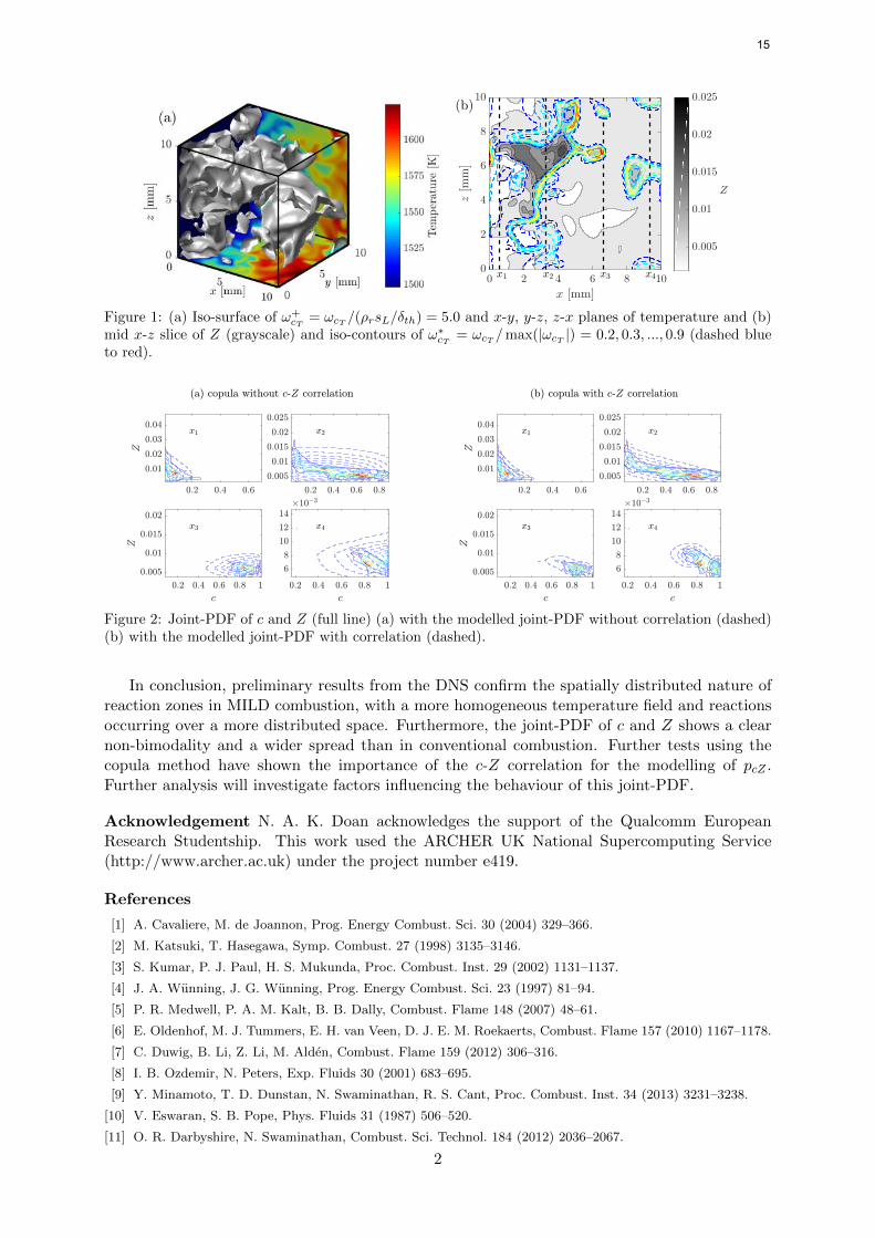
= 20m/s.In Fig. 1a, the temperature field and the iso-surface of normalized reaction rate of c, noted as

!

+cT, is represented. It is observed that the reaction zones have a complex morphology, extremely

di↵erent from the conventional cases. The reaction zone is distributed over the entire compu-tational volume which confirms the earlier experimental observations of spatially distributedreaction zones [2, 4]. A cut through the mid x-z plane is depicted in Fig. 1b showing Z ingrayscale and !

cT as contour lines. One observes that the reacting regions present an extremelyconvoluted aspect with some of them seemingly wrapped around the pocket of rich mixtures.The influence of the gradient of Z on the structure and morphology of the reaction zones remainsto be analysed and understood.

The joint probability density function (PDF), pcZ

, of the progress variable c and Z at variousx-locations is shown in Fig. 2. At x1 location, it can be observed that Z presents a range ofvalue and that most mixture is in an unburned state as depicted by the low c. At x2 location,the range of Z has narrowed under the e↵ect of turbulent mixing and the PDF of c shows aspread and not a clear bimodal character as would be found in premixed flames. This spreadof c is due to multiple e↵ects. First, heat is di↵used from the reacting zones towards thepockets of products coming from the inlet. Second, the presence of a range of mixture fractioninduces various ignition delay times, which leads to this spread in progress variable at a given x-location. Further downstream, the range of mixture fractions is even further narrowed under theinfluence of turbulent mixing and the range of c shows that most of the mixture has completelyreacted. As a first attempt towards modelling p

cZ

, the joint-PDF modelled using the copula

method proposed in [11] is presented with c-Z correlation (Fig. 2b) extracted from the DNSand without this correlation (Fig. 2a). It is observed that including the correlation gives asubstantial improvements on the modelled joint-PDF as one would expect.

aCorresponding email: nakd2@cam.ac.uk1

14

x1 x2 x3 x4

(b)

0 2 4 6 8 10

x [mm]

0

2

4

6

8

10

z[m

m]

0.005

0.01

0.015

0.02

0.025

Z

Figure 1: (a) Iso-surface of !+cT = !cT /(⇢rsL/�th) = 5.0 and x-y, y-z, z-x planes of temperature and (b)

mid x-z slice of Z (grayscale) and iso-contours of !⇤cT = !cT /max(|!cT |) = 0.2, 0.3, ..., 0.9 (dashed blue

to red).

x1

0.2 0.4 0.6

0.01

0.02

0.03

0.04

Z

x2

0.2 0.4 0.6 0.8

0.005

0.01

0.015

0.02

0.025

x3

0.2 0.4 0.6 0.8 1

c

0.005

0.01

0.015

0.02

Z

(a) copula without c-Z correlation

x4

0.2 0.4 0.6 0.8 1

c

6

8

10

12

14#10!3

x1

0.2 0.4 0.6

0.01

0.02

0.03

0.04

Z

x2

0.2 0.4 0.6 0.8

0.005

0.01

0.015

0.02

0.025

x3

0.2 0.4 0.6 0.8 1

c

0.005

0.01

0.015

0.02

Z

(b) copula with c-Z correlation

x4

0.2 0.4 0.6 0.8 1

c

6

8

10

12

14#10!3

Figure 2: Joint-PDF of c and Z (full line) (a) with the modelled joint-PDF without correlation (dashed)(b) with the modelled joint-PDF with correlation (dashed).

In conclusion, preliminary results from the DNS confirm the spatially distributed nature ofreaction zones in MILD combustion, with a more homogeneous temperature field and reactionsoccurring over a more distributed space. Furthermore, the joint-PDF of c and Z shows a clearnon-bimodality and a wider spread than in conventional combustion. Further tests using thecopula method have shown the importance of the c-Z correlation for the modelling of p

cZ

.Further analysis will investigate factors influencing the behaviour of this joint-PDF.

Acknowledgement N. A. K. Doan acknowledges the support of the Qualcomm EuropeanResearch Studentship. This work used the ARCHER UK National Supercomputing Service(http://www.archer.ac.uk) under the project number e419.

References

[1] A. Cavaliere, M. de Joannon, Prog. Energy Combust. Sci. 30 (2004) 329–366.

[2] M. Katsuki, T. Hasegawa, Symp. Combust. 27 (1998) 3135–3146.

[3] S. Kumar, P. J. Paul, H. S. Mukunda, Proc. Combust. Inst. 29 (2002) 1131–1137.

[4] J. A. Wunning, J. G. Wunning, Prog. Energy Combust. Sci. 23 (1997) 81–94.

[5] P. R. Medwell, P. A. M. Kalt, B. B. Dally, Combust. Flame 148 (2007) 48–61.

[6] E. Oldenhof, M. J. Tummers, E. H. van Veen, D. J. E. M. Roekaerts, Combust. Flame 157 (2010) 1167–1178.

[7] C. Duwig, B. Li, Z. Li, M. Alden, Combust. Flame 159 (2012) 306–316.

[8] I. B. Ozdemir, N. Peters, Exp. Fluids 30 (2001) 683–695.

[9] Y. Minamoto, T. D. Dunstan, N. Swaminathan, R. S. Cant, Proc. Combust. Inst. 34 (2013) 3231–3238.

[10] V. Eswaran, S. B. Pope, Phys. Fluids 31 (1987) 506–520.

[11] O. R. Darbyshire, N. Swaminathan, Combust. Sci. Technol. 184 (2012) 2036–2067.

2

15

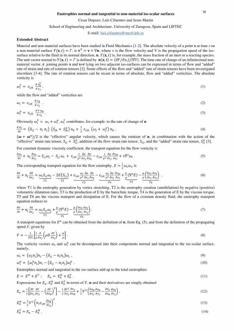
Enstrophies normal and tangential to non-material iso-scalar surfaces Cesar Dopazo, Luis Cifuentes and Jesus Martin

School of Engineering and Architecture, University of Zaragoza, Spain and LIFTEC E-mail: luis.cifuentes@mech.kth.se

Extended Abstract Material and non-material surfaces have been studied in Fluid Mechanics [1-2]. The absolute velocity of a point x at time t on a non-material surface 𝑌(𝐱, 𝑡) = 𝛤, is 𝐯Y = 𝐯 + V𝐧, where v is the flow velocity and V is the propagation speed of the iso-surface relative to the fluid in its normal direction, n. 𝑌(𝐱, 𝑡) is, for example, the mass fraction of an inert or a reacting species. The unit vector normal to 𝑌(𝐱, 𝑡) = 𝛤 is defined by 𝐧(𝐱, t) = (𝜕𝑌/𝜕𝑥𝑖)/|∇𝑌|. The time rate of change of an infinitesimal non-material vector, r, joining points x and x+r lying on two adjacent iso-surfaces can be expressed in terms of flow and “added” rate of strain and rate of rotation tensors [3]. Some effects of the flow and “added” rate of strain tensors have been investigated elsewhere [3-4]. The rate of rotation tensors can be recast in terms of absolute, flow and “added” vorticities. The absolute vorticity is

𝜔𝑖𝑌 = 𝜀𝑖𝑗𝑘 𝜕 v𝑘𝑌

𝜕 𝑥𝑗 , (1)

while the flow and “added” vorticities are

𝜔𝑖 = 𝜀𝑖𝑗𝑘 𝜕 v𝑘𝜕 𝑥𝑗 , (2)

𝜔𝑖𝑎 = 𝜀𝑖𝑗𝑘 𝜕 𝑉 𝑛𝑘𝜕 𝑥𝑗 . (3)

Obviously 𝜔𝑖𝑌 = 𝜔𝑖 + 𝜔𝑖𝑎. 𝜔𝑖𝑌 contributes, for example, to the rate of change of n 𝑑 𝑛𝑖𝑑𝑡 = (𝛿𝑖𝑗 − 𝑛𝑖 𝑛𝑗) (𝑆𝑗𝑘 + 𝑆𝑗𝑘

𝑎 ) 𝑛𝑘 + 12 𝜀𝑖𝑗𝑘 (𝜔𝑗 + 𝜔𝑗𝑎) 𝑛𝑘 , (4)

(𝝎 + 𝝎𝑎)/2 is the “effective” angular velocity, which causes the rotation of n, in combination with the action of the “effective” strain rate tensor, 𝑆𝑖𝑗 + 𝑆𝑖𝑗𝑎 , addition of the flow strain rate tensor, 𝑆𝑖𝑗 , and the “added” strain rate tensor, 𝑆𝑖𝑗𝑎 [3].

For constant dynamic viscosity coefficient, the transport equation for the flow vorticity is 𝜕𝜔𝑖𝜕𝑡 + 𝑢𝑗

𝜕𝜔𝑖𝜕𝑥𝑗

= 𝑆𝑖𝑗𝜔𝑗 − 𝑆𝑗𝑗 𝜔𝑖 + 𝜀𝑖𝑗𝑘 1𝜌2

𝜕𝜌𝜕𝑥𝑗

𝜕𝑝𝜕𝑥𝑘

− 𝜀𝑖𝑗𝑘 1𝜌2

𝜕𝜌𝜕𝑥𝑗

𝜕𝜏𝑘𝑙𝜕𝑥𝑙

+ 𝜈∇2𝜔𝑖 . (5)

The corresponding transport equation for the flow enstrophy, 𝐸 = 12𝜔𝑖𝜔𝑖, is

𝜕𝐸𝜕𝑡 + 𝑢𝑗

𝜕𝐸𝜕𝑥𝑗= 𝜔𝑖𝑆𝑖𝑗𝜔𝑗⏟

𝑇1− 2𝐸(𝑆𝑗𝑗)⏟

𝑇2+ 𝜀𝑖𝑗𝑘 𝜔𝑖𝜌2

𝜕𝜌𝜕𝑥𝑗

𝜕𝑝𝜕𝑥𝑘⏟

𝑇3

− 𝜀𝑖𝑗𝑘 𝜔𝑖𝜌2𝜕𝜌𝜕𝑥𝑗

𝜕𝜏𝑘𝑙𝜕𝑥𝑙⏟

𝑇4

+ 𝜇𝜌 (∇

2𝐸)⏟ 𝑇5

− 𝜇𝜌 (

𝜕𝜔𝑖𝜕𝑥𝑗

𝜕𝜔𝑖𝜕𝑥𝑗)⏟

𝑇6

, (6)

where T1 is the enstrophy generation by vortex stretching, T2 is the enstrophy creation (annihilation) by negative (positive) volumetric dilatation rates, T3 is the production of E by the baroclinic torque, T4 is the generation of E by the viscous torque, T5 and T6 are the viscous transport and dissipation of E. For the flow of a constant density fluid, the enstrophy transport equation reduces to 𝜕𝐸𝜕𝑡 + 𝑢𝑗

𝜕𝐸𝜕𝑥𝑗= 𝜔𝑖𝑆𝑖𝑗𝜔𝑗⏟

𝑇1+ 𝜇𝜌 (∇

2𝐸)⏟ 𝑇5

− 𝜇𝜌 (

𝜕𝜔𝑖𝜕𝑥𝑗

𝜕𝜔𝑖𝜕𝑥𝑗)⏟

𝑇6

. (7)

A transport equations for 𝐸𝑎 can be obtained from the definition of n, from Eq. (5), and from the definition of the propagating speed,V, given by

𝑉 = − 1|∇𝑌| [

1𝜌𝜕𝜕𝑥𝑗(𝜌𝐷 𝜕𝑌

𝜕𝑥𝑗) + 𝑤

𝜌] . (8)

The vorticity vectors 𝜔𝑖 and 𝜔𝑖𝑎 can be decomposed into their components normal and tangential to the iso-scalar surface, namely, 𝜔𝑖 = (𝜔𝑗𝑛𝑗)𝑛𝑖 − (𝛿𝑖𝑗 − 𝑛𝑖𝑛𝑗)𝜔𝑗 , (9)

𝜔𝑖𝑎 = (𝜔𝑗𝑎𝑛𝑗)𝑛𝑖 − (𝛿𝑖𝑗 − 𝑛𝑖𝑛𝑗)𝜔𝑗𝑎 . (10)

Enstrophies normal and tangential to the iso-surface add up to the total enstrophies 𝐸 = 𝐸𝑁 + 𝐸𝑇 ; 𝐸𝑎 = 𝐸𝑎𝑁 + 𝐸𝑎𝑇 . (11) Expressions for 𝐸𝑎, 𝐸𝑎𝑁 and 𝐸𝑎𝑇 in terms of 𝑉, n and their derivatives are simply obtained

𝐸𝑎 = 12 [

𝜕𝑉𝜕𝑥𝑗

𝜕𝑉𝜕𝑥𝑗− ( 𝜕𝑉𝜕𝑥𝑁)

2] − 1

2𝜕𝑉2𝜕𝑥𝑗

𝜕𝑛𝑗𝜕𝑥𝑁

+ 12𝑉

2 (𝜕𝑛𝑘𝜕𝑥𝑗𝜕𝑛𝑘𝜕𝑥𝑗

− 𝜕𝑛𝑗𝜕𝑥𝑘

𝜕𝑛𝑘𝜕𝑥𝑗) , (12)

𝐸𝑎𝑁 = 12 𝑉

2 (𝑛𝑖𝜀𝑖𝑗𝑘 𝜕𝑛𝑘𝜕𝑥𝑗)2, (13)

𝐸𝑎𝑇 = 𝐸𝑎 − 𝐸𝑎𝑁 . (14)

16

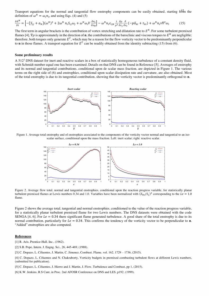
Transport equations for the normal and tangential flow enstrophy components can be easily obtained, starting from the definition of 𝜔𝑁 = 𝜔𝑖𝑛𝑖, and using Eqs. (4) and (5) 𝐷𝐸𝑁𝐷𝑡 = [−(𝑆𝑗𝑗 + 𝑎𝑁)(𝜔

𝑁)2 + 2𝜔𝑁 𝑛𝑖𝑆𝑖𝑗𝜔𝑗 + 𝜔𝑁𝜔𝑖𝑉 𝜕𝑛𝑖𝜕𝑥𝑁] − 𝜔𝑁𝑛𝑖𝜀𝑖𝑗𝑘 1

𝜌2𝜕𝜌𝜕𝑥𝑗

𝜕𝜕𝑥𝑙(−𝑝𝛿𝑘𝑙 + 𝜏𝑘𝑙) + 𝜔𝑁𝑛𝑖𝜈∇2𝜔𝑖 (15)

The first term in angular brackets is the contribution of vortex stretching and dilatation rate to 𝐸𝑁. For some turbulent premixed flames [4], ∇𝜌 is approximately in the direction of n, the contributions of the baroclinic and viscous torques to 𝐸𝑁 are negligible; therefore, both torques only generate 𝐸𝑇, which may be a reason for the flow vorticity vector to be predominantly perpendicular to n in those flames. A transport equation for 𝐸𝑇 can be readily obtained from the identity subtracting (15) from (6). Some preliminary results A 5123 DNS dataset for inert and reactive scalars in a box of statistically homogeneous turbulence of a constant density fluid, with Schmidt number equal one has been examined. Details on that DNS can be found in Reference [5]. Averages of enstrophy and its normal and tangential contributions, conditional upon de scalar mass fraction, are depicted in Figure 1. The various terms on the right side of (6) and enstrophies, conditional upon scalar dissipation rate and curvature, are also obtained. Most of the total enstrophy is due to its tangential contribution, showing that the vorticity vector is predominantly orthogonal to n.

Figure 1. Average total enstrophy and of enstrophies associated to the components of the vorticity vector normal and tangential to an iso-

scalar surface, conditional upon the mass fraction. Left: inert scalar; right: reactive scalar.

Figure 2. Average flow total, normal and tangential enstrophies, conditional upon the reaction progress variable, for statistically planar turbulent premixed flames at Lewis numbers 0.34 and 1.0. Variables have been normalized with (𝛿𝑡ℎ/𝑆𝐿)2 corresponding to the 𝐿𝑒 = 1.0 flame.

Figure 2 shows the average total, tangential and normal enstrophies, conditioned to the value of the reaction progress variable, for a statistically planar turbulent premixed flame for two Lewis numbers. The DNS datasets were obtained with the code SENGA [4, 6]. For 𝐿𝑒 = 0.34 there significant flame generated turbulence. A good share of the total enstrophy is due to its normal contribution, particularly for 𝐿𝑒 = 0.34. This confirms the tendency of the vorticity vector to be perpendicular to n. “Added” enstrophies are also computed. References [1] R. Aris, Prentice-Hall, Inc., (1962). [2] S.B. Pope, Intern. J. Engng. Sci., 26, 445-469, (1988). [3] C. Dopazo, L. Cifuentes, J. Martin, C. Jimenez, Combust. Flame, vol. 162, 1729 – 1736, (2015). [4] C. Dopazo, L. Cifuentes and N. Chakraborty, Vorticity budgets in premixed combusting turbulent flows at different Lewis numbers, (submitted for publication). [5] C. Dopazo, L. Cifuentes, J. Hierro and J. Martin, J. Flow, Turbulence and Combust, pp 1, (2015). [6] K.W. Jenkins, R.S Cant, in Proc. 2nd AFOSR Conference on DNS and LES, p192, (1999).

17

Mixture fraction-progress variable dependence in partially-premixed flames

Tomas B. Matheson and Edward S. Richardsona

Faculty of Engineering and the Environment, University of Southampton, Southampton, SO17 1BJ, UK

It is both convenient and conventional to assume that mixture fraction and progress variable are statistically independent in turbulent partially-premixed combustion modelling. This assumption simplifies presumed-probability density function (pdf) modelling for the joint mixture fraction–progress variable pdf, implying that it can be expressed as the product of the marginal-pdf of mixture fraction and the marginal-pdf of progress variable,

𝑝ξ,c(𝜂,𝜁) = 𝑝ξ(𝜂)𝑝c(𝜁), (1) where 𝜂 and 𝜁 are the sample space variables for mixture fraction ξ and progress variable c respectively. The assumption of statistical independence can give adequate model predictions in some circumstances, however there is no general theoretical basis for assuming statistical independence between mixture fraction and progress variable, and the limitations of the assumption of statistical independence are not well established. The objective of this study is to use statistical analysis of empirical joint mixture fraction–progress variable pdfs, obtained from laboratory and Direct Numerical Simulation (DNS) data for partially-premixed combustion, in order to characterise the mixture fraction–progress variable dependence. Three turbulent combustion data sets shown in Fig. 1 are considered: first, DNS data for equivalence ratio-stratified flame propagation in the thin reaction zones regime [1]; second, laboratory data for a non-premixed jet flame with significant levels of localised extinction [2]; and third, DNS data for an autoigniting slot jet flame [3].

Figure 1: (left) Equivalence ratio stratified combustion DNS showing volume rendering of heat release coloured by mixture fraction [1]; (centre) long-exposure close up photograph of the Sandia Flame D pilot [2]; (right) cross section through the OH mass fraction field in autoigniting ethylene jet flame DNS [3]. The statistical dependence of the two variables is visualised by defining a mathematical transformation of the data in order to remove the contributions of the marginal distributions, as illustrated in Fig. 2. The influence of the statistical dependence on the evaluation of statistical moments, such as mean reaction rates predicted in conjunction with flamelet modelling, are then evaluated by integrating the flamelet properties over (a) the empirical joint-pdf, (b) the independent joint-pdf based on the empirical marginal pdfs based on Eq. 1, or (c) a modelled joint-pdf with statistical dependence specified by the Plackett copula and the empirical covariance [4].

a e.s.richardson@soton.ac.uk

18

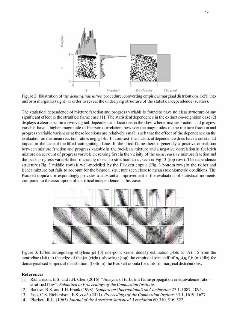
. Figure 2: Illustration of the demarginalisation procedure, converting empirical marginal distributions (left) into uniform marginals (right) in order to reveal the underlying structure of the statistical dependence (scatter). The statistical dependence of mixture fraction and progress variable is found to have no clear structure or any significant effect in the stratified flame case [1]. The statistical dependence in the extinction-reignition case [2] displays a clear structure involving tail-dependence at locations in the flow where mixture fraction and progress variable have a higher magnitude of Pearson correlation, however the magnitudes of the mixture fraction and progress variable variances at these locations are relatively small, such that the effect of the dependence on the evaluation on the mean reaction rate is negligible. In contrast, the statistical dependence does have a substantial impact in the case of the lifted autoigniting flame. In the lifted flame there is generally a positive correlation between mixture fraction and progress variable in the fuel-lean mixture and a negative correlation in fuel-rich mixture on account of progress variable increasing first in the vicinity of the most reactive mixture fraction and the peak progress variable then migrating closer to stoichiometric, seen in Fig. 3 (top row). The dependence structure (Fig. 3 middle row) is well-modelled by the Plackett copula (Fig. 3 bottom row) in the richer and leaner mixture but fails to account for the bimodal structure seen close to mean stoichiometric conditions. The Plackett copula correspondingly provides a substantial improvement in the evaluation of statistical moments compared to the assumption of statistical independence in this case.

Figure 3: Lifted autoigniting ethylene jet [3] one-point kernel density estimation plots at x/H=15 from the centreline (left) to the edge of the jet (right), showing: (top) the empirical joint-pdf of 𝑝ξ,c(𝜂, 𝜁); (middle) the demarginalised empirical distribution; (bottom) the Plackett copula for uniform marginal distributions. References [1] Richardson, E.S. and J.H. Chen (2016). “Analysis of turbulent flame propagation in equivalence ratio-

stratified flow”. Submitted to Proceedings of the Combustion Institute. [2] Barlow, R.S. and J.H. Frank (1998). Symposium (International) on Combustion 27.1. 1087–1095. [3] Yoo, C.S, Richardson, E.S. et al. (2011). Proceedings of the Combustion Institute 33.1, 1619–1627. [4] Plackett, R.L. (1965) Journal of the American Statistical Association 60.310, 516–522.

19

1

Effects of residence time on flame speed in autoignitive mixtures of methane and n-heptane

Bruno S. Soriano, Tomas B. Matheson, and Edward S. Richardson1

Faculty of Engineering and the Environment, University of Southampton, Southampton, SO17 1BJ,

UK

Natural gas can be used to power compression-ignition engines via the dual-fuel mode, where a more reactive fuel such as diesel is also injected in order to provide a source of ignition [1]. Following ignition, flame propagates through a partially-reacted inhomogeneous mixture of the two fuels in which deflagration and ignition fronts can be present [2,3]. Flame propagation through dual-fuel blends is especially significant in non-premixed dual-fuel engines in which both fuels are directly injected at the end of compression. The kinetic coupling between methane and n-heptane fuels is shown to have a significant influence on both ignition and flame propagation at compression-ignition engine conditions, which chemical mechanisms and flame-speed models should take into account. In particular, we quantify and then model how preignition chemistry of the dual-fuel mixtures accelerates flame propagation in two stages that correspond to the two stages of autoignition in diesel-like fuels. Methodology Flame propagation through methane and n-heptane fuel blends is studied using numerical simulations. A set of freely propagating and burner stabilised one-dimensional laminar flame simulations are used to investigate the effects of methane/n-heptane ratios and residence time on flame speed at engine-relevant temperatures and pressures. The flames are simulated using the COSILAB one-dimensional premixed flame solver [4] with multicomponent molecular transport and semi-perfect gas models for thermodynamic properties. Thermal radiation is neglected. The numerical solution uses adaptive grid refinement based on all variables and a modified-Newton method. In the freely-propagating case, the residence-time at the flame location is varied by changing the length of the simulation domain upstream of the flame front, as in [5], while in the burner stabilised flame the residence time is changed by setting different inlet velocities in a domain big enough to stabilise the flame. The results of the freely propagating and burner stabilised flames are consistent, however the use of the burner stabilised flame configuration facilitates numerical solution of flames that exhibit a so-called cool-flame (due to first-stage ignition) ahead of the main flame front. The residence time corresponds to the convective time upstream of the flame location within the solution domain: 𝜏𝑐𝑜𝑛𝑣.=∫1/𝑢𝑥. 𝑑𝑥, where 𝑢𝑥 is the convection velocity. Several detailed and reduced chemical kinetic models are compared in terms of ignition delays and flame speeds for various fuel mixtures and conditions. The POLIMI_NC7_106 reduced mechanism [6] is adopted for the subsequent investigations of methane/n-heptane combustion behaviour. Reactant mixtures are described in terms of their total-equivalence ratio, 𝜙𝑡𝑜𝑡, evaluated in the conventional manner by considering the stoichiometric oxygen-fuel ratio for the fuel mixture, and fuel-equivalence ratios, 𝜙CH4 = 𝜈CH4𝑌CH4,u/𝑌O2,u and 𝜙C7H16 = 𝜈C7H16𝑌C7H16,u/𝑌O2,u , where subscript 𝑢 denotes the unburnt composition and 𝜈i is the stoichiometric oxygen-to-fuel mass ratio for the 𝑖𝑡ℎ fuel species, such that 𝜙𝑡𝑜𝑡 = 𝜙CH4 + 𝜙C7H16. Results 1 e.s.richardson@soton.ac.uk

20

2

The effects of pre-ignition chemistry on flame speed are investigated, revealing that fuel blends that exhibit two-stage ignition also exhibit a two-stage increase in flame speed as the residence time of the fuel-air mixture increases. In Fig. 1 the flame speed has a sharp increase when the residence time reaches the first-stage ignition delay time; then increases gradually during the second-stage ignition-delay; before increasing indefinitely as the residence time approaches final ignition delay time. In turbulent combustion models that use laminar flame speed as a parameter, flame acceleration due to pre-ignition reactions is an important phenomenon that should be included in flame speed models. The analysis indicates that the increase in flame speed during first-stage ignition is due to the combined effect of the chemical species and the temperature-rise produced by the first-stage ignition. The numerical tests are performed that demonstrate that methane addition acts to suppress radical formation and to decrease the flame speed dependence on residence time.

Subsequently a laminar flame speed model for methane–n-heptane blends is developed to account for the variation of the fuel blend, and extended to account for the heat released and fuel consumed during first-stage ignition. Out of several fuel mixing rules for modelling flame speed that were analysed, a linear mixing rule presented a better accuracy for evaluating the flame speed of fuel blends and is adopted in this study. The Metghalchi and Keck [7] flame speed correlation format is used to calculate the dependence of flame speed on the unburnt temperature, pressure, equivalence ratio and the mass fraction ξ of diluents for each fuel. The model constants are obtained using least-squares fitting in a set of 45 flames for each fuel. The flame speed increase due to two-stage ignition is captured by means of a progress variable c based on temperature. The new model is validated in Fig. 1 for a range of fuel blends, adequately capturing the main thermal effect of pre-ignition chemistry but, since this model does not account for the presence of pre-ignition radicals it under-predicts the flame speed during first-stage ignition.

References [1] T. Korakianitis, A. M. Namasivayam and R. J. Crookes, Prog. Energy Combust. Sci. 37 (2011) 89-112. [2] E. Demosthenous, G. Borghesi, E. Mastorakos and R. S. Cant, Combust. Flame. In press., (2015). [3] Z. Wang and J. Abraham, Proc. Combust. Inst. 35 (2015) 1041-1048. [4] Cosilab, Rotexo Software, Bochum, 2011. [5] P. Habisreuther, F. C. C. Galeazzo, C. Prathap and N. Zarzalis, Combust. Flame, 160 (2013) 2770-2782.

21

3

[6] E. Ranzi, A. Frassoldati, A. Stagni, M. Pelucchi, A. Cuoci and T. Faravelli, Int. J. Chem. Kinet. 46(9) (2014) 512-542. [7] M. Metghalchi and J. C. Keck, Combust. Flame 48 (1982) 191-210.

22

Joint British, Spanish and Portuguese Section Combustion Institute Meeting - 12-13th April 2016 Cambridge(UK)

THERMAL VALORIZATION OF SUB-BITUMINOUS WASTE COAL IN A 160MWe UTILITY BOILER: A CFD ANALYSIS

Carlos Herce*, Javier Pallarés, Carmen Bartolomé, Cristóbal Cortés

Research Centre for Energy Resources and Consumption (CIRCE) - Universidad de Zaragoza C/ Mariano Esquillor Gómez, 15, 50018 Zaragoza, Spain; Email*: cherce@unizar.es

ABSTRACT Coal combustion supplies the 26.7% of electricity generated in EU-28. In 2014, the 36% of gross inland consumption was covered by regional extracted coal, a strong reduction compared with 74% in 1990. During coal mining a variable amount of material is rejected due to present a considerable content of inert mineral mixed with coal. This solid mining refuse is usually called waste coal, and it is specifically referred to as "culm" in the anthracite fields and as "gob" in the bituminous coal mining regions. In Europe the waste coal was for decades disposed in landfills, with all the security measurements in order to minimize environmental impacts (mainly acidity and contamination with sulphur and heavy metals). However, in the last years several national and European directives have been promoted to recycle and valorize the waste coal. Thermal valorization of coal waste is one of the most extended options [1]. Nowadays, in U.S. exists 18 plants that uses waste coal as primary fuel and 13 plants that uses as secondary fuel, mainly in fluidized bed boilers at very different sizes (from 30 to 2800 MWe). However, in EU it is not implemented. On the one hand, due to the high European electricity prices, it is difficult to assume the increase of operation cost. On the other hand, most of the plants in the European power park (mainly the older ones) are based in pulverized coal technologies, where it is difficult to operate with alternative fuels. The aim of this work is to evaluate the technical feasibility of co-firing of coal with waste coal gob from Teruel coalfields, in the PC Escucha power plant by means of numerical simulations. Gob presents a very high ash content (45%), a high sulphur concentration (at least 3%), and a small heating value (LHV=8700 kJ/kg). However, this fuel offers a very promising potential in agrochemical industry. Particularly the ashes presents a very high content on iron (30%) that can be used as subtract of fertilizer, and, the sulphur oxides produced during the combustion process can be condensed to produce sulfuric acid. Thus the thermal valorization, instead of the relatively low potential to power generation, provides a complete cycle of reuse of byproducts. This paper presents a numerical investigation, using CFD techniques, on the effect of co-firing in a 160MWe utility boiler. A comprehensive numerical model has been carried out including an Eurelian-Lagrangian approximation to solve the coupling of gas and particulate phase (two-way coupling), using a steady RANS approach along the computational domain and making use of the standard κ–ε model to close the turbulence problem. Radiative heat transfer has been modeled using P-1 model, with WSGGM to estimate the absorption coefficient. A 3D hybrid structured-polyhedral mesh formed by 210,000 cells has been made up to obtain a good compromise between computational cost and accuracy. The three mechanisms (devolatilization, volatiles combustion and char oxidation) involved in coal combustion have been considered [2]. In this work, three different options of direct-co-firing are proposed. Firstly, mixing gob with coal previously to milling process; by means of this approach both fuels are homogenous introduced to the burners. Secondly, to use a dedicated burner to gob instead of coal in the upper row of burners (B2), and thirdly, burning gob in a burner placed in the middle of the burners wall (D2). Three different substitution rates have been evaluated: 0% (corresponding to 100% coal combustion), 6.25% (a single burner power, 30 MW), and 12.5% (two burners substitution). Additionally, in order to evaluate the effect of devolatilization kinetic parameters in combustion process, five simulations using kinetics literature data have been compared with kinetics derived from TGA [3]. Results have been validated with plant data (only coal case) with a good agreement [4]. The main global simulation results are presented in Table 1 and some local results and differences are shown in Fig. 1. Strong differences have been observed due to kinetic parameters of devolatilization. Moreover, the co-firing (in the substitution percentages considered) not affects critically to the

23

Joint British, Spanish and Portuguese Section Combustion Institute Meeting - 12-13th April 2016 Cambridge(UK)

efficiency of the boiler. Additionally, several improvements in the operation can be derived from simulation results (e.g. being homogeneous combustion the best option, combustion in dedicated burner in the upper row presents a better efficiency than in bottom one).

ACKNOWLEDGMENTS The work presented in this paper has been partially supported by the research project “Reconversión de centrales térmicas de carbón mediante valorización energética de escombreras y aprovechamiento integral de residuos” funded by the Spanish Ministry of Science and Innovation in the INNPACTO programme (IPT-2012-0251-120000).

REFERENCES [1] La Nauze, R.D., Duffy, G.J. (1987) Environmental Geochemistry and Health, 7 (2) 69-79 [2] Pallarés, J. et al. (2009) Fuel Processing Technology, 90 (10) 1207-1213 [3] Herce, C. et al. (2014) Journal of Thermal Analysis and Calorimetry, 117 (1) 507-516 [4] Canalis, P (2012). PhD Thesis. University of Zaragoza. 2012.  

Table 1. Temperature, composition of the product gases and fuel conversion at the boiler exit

N. Code Co-

firing burners

Sub. (%)

Tout (ºC)

O2 (%)

CO2 (%)

CO (%)

H2O(%)

SO2 (%)

SO3(%) Coal

Conversion (%)

Gob conversion

(%) 1 C_0_- -------- 0 1268 4,5 16 0,002 4,6 0,19 1,50E-03 99,99 -

2 A_6_- ALL 6,25 1236 4,6 16,9 0,170 4,6 0,3 1,90E-03 99,18 99,22

3 A_12_- ALL 12,5 1225 4,,8 15,4 0,016 4,6 0,37 2,63E-03 99,53 99,49

4 B2_100_- B2 6,25 1242 4,7 15,6 0,150 4,6 0,3 1,80E-03 100 97,1

5 D2_100_- D2 6,25 1230 4,8 15,6 0,070 4,6 0,28 2,34E-03 99,13 98,08

6 C_0_K -------- 0 1269 4,6 15,9 0,001 4,6 0,2 1,50E-03 99,89 -

7 A_6_K ALL 6,25 1235 4,8 16,4 0,150 4,6 0,28 1,84E-03 99,1 100

8 A_12_K ALL 12,5 1216 4,8 15,4 0,150 4,6 0,38 2,65E-03 99,42 99,75

9 B2_100_K B2 6,25 1510 4,8 15,5 0,130 4,6 0,28 1,87E-03 98,25 90,85 10 D2_100_K D2 6,25 1497 4,8 15,4 0,160 4,6 0,27 2,07E-03 99,33 98,6

 

 

Figure 1. Temperature profiles at a) different substtituion rates b) 6.25% gob in different burner configurations and c) effect of different kinetic parameters (-, Kinetics form literature; K-Kinetics from TGA)

24

Thermal degradation effects of the atmosphere and lid used in STA test for thermoplastic polymers

David Lázaro, Mariano Lázaro, Daniel Alvear

University of Cantabria. School of Industrial Engineering, Avenue of Los Castros s/n Santander, 39005 Spain

Abstract Experimental analysis of polymer thermal degradation using methods based on thermogravimetric analysis (TGA) and differential scanning calorimetry (DSC) are widely used. These apparatuses are conditioned by sample size (milligram scale), but allow to define different boundary conditions to tests the samples. Results of these tests are widely dependent of the boundary conditions that user select to perform the tests. Heat ramp defined by the user affect the instant and temperature at which the different reaction takes places. The atmosphere can be air or inert one, to allow or avoid different reactions. STA measurements can be done with or without lid. The use of the lid will affect test results, so it is necessary to know how can it affect to each material before perform the test. In [1] it is recommended the use of lid to avoid radiation corrections to the global signal when temperatures are high enough. However, there are some results for wood [2] and also gypsum [3] that showing clearly the interaction of solid with the gas products of its own gasification. Furthermore, when oxidation atmospheres are performed combustion of gases yielded can modify the DSC signal as suggested Peterson et al. [4]. A series of tests varying the atmosphere in the furnace of the STA, and with and without lid in the holder, were developed in order to better understand lid effect in test results. PVC and LLDPE were employed in the study in order to study the effect in two kind of thermoplastics. Table 1 shows the boundary conditions of the tests.

Table 1 Boundary conditions of STA tests.

Material Heat rate Atmosphere Lid PVC 10 20 % O2 / 80 % N2 Yes

10 20 % O2 / 80 % N2 No 10 10 % O2 / 90 % N2 No 10 5 % O2 / 95 % N2 No 10 100 % N2 Yes 10 100 % N2 No

LLDPE 10 20 % O2 / 80 % N2 Yes 10 20 % O2 / 80 % N2 No 10 10 % O2 / 90 % N2 No 10 100 % N2 Yes 10 100 % N2 No

Fig 1 and 2 show some of the test results that allow to observe how lid affect mainly to oxidant reaction that takes place in the reactant atmosphere. On the one hand, the effect shown on inert atmosphere is very low and can be related to the radiation effect. Mass lost and energy release are mainly the same. The pinhole lid allows the same pressure in the test independently of lid. In addition, when inert atmosphere is considered, it is not relevant the surrounding atmosphere in the degradation of the sample.

25

By the other hand, lid limits the reactions in the thermoplastics under reactant atmosphere. The energy release in the reactions decrease with the lid, because the gases released in the degradation fill the holder, and avoid oxygen enter in the holder, and so on, complete oxidation reactions to take place.

Fig. 1. Percent mass loss (TG) and heat flux (DSC) for oxidant (left side) and nitrogen atmospheres for

LLDPE.

Fig. 2. Percent mass loss (TG) and heat flux (DSC) for oxidant (left side) and nitrogen atmospheres for PVC.

ACKNOWLEDGEMENTS The authors of this study would like to thank to the Spanish Ministry of Economy and Competitiveness for the PYRODESIGN and EVACTRAIN Project grant, Ref.: BIA2012-37890 and TRA2011-26738 respectively, financed jointly by FEDER funds. REFERENCES [1] A.T.W. Kempen, F. Sommer, E.J. Mittemeijer, The isothermal and isochronal kinetics of the crystallization of bulk amorphous Pd40Cu30P20Ni10, Acta Materialia 50 (2002) 1319–1329. [2] M.G Wolfinger, J Rath, G Krammer, F Barontini, V Cozzani, Influence of the emissivity of the sample on differential scanning calorimetry measurements, Thermochimica Acta 372 (2001) 11–18. [3] W. Lou, B. Guan, Z. Wu, Dehydration behavior of FGD gypsum by simultaneous TG and DSC analysis, J Therm Anal Calorim 104 (2011) 661–669. [4] J. D. Peterson, S. Vyazovkin, C. A. Wight, Kinetics of the Thermal and Thermo-OxidativeDegradation of Polystyrene, Polyethylene andPoly(propylene), Macromol. Chem. Phys. 202 (2001) 775–784.

26

Material pyrolysis estimation combining mass and energy as optimization targets

Alonso, A.; Lázaro, D; Lázaro, M.; Alvear, D. GIDAI Group - Fire Safety - Research and Technology. University of Cantabria. (Spain)

ABSTRACT

The pyrolysis processes, according to Arrhenius equation [1], are mainly governed by activation energy (E), pre-exponential factor (A), reaction order (௦). They are usually known as kinetic parameters. Thermal analysis techniques provide TGA and DSC curves that describe the pyrolysis process, but do not provide the values of the kinetic parameters which are intended for fire modelling. In order to obtain them, optimization algorithms are extensively used. The work of Pello and Lautemberger [2] compiles briefly some contributions in this area.

These previous works look forward to determining how closely we can reproduce the actual material pyrolysis but the principal or unique optimization target used is the mass loss rate (TGA curve) instead of the study of the energy released that is a decisive aspect of fire protection engineering.

On this basis, this work proposes add a new target to estimate pyrolysis properties: the study of DSC curve, so the thermal properties will be achieved fitting experimental and simulated of TGA and DSC curves simultaneously.

Several commercial materials were studied: Experimental curves were obtained by STA analyses at different levels of oxygen concentration, either reactive (air atmosphere) or inert (Nitrogen atmosphere). To estimate the kinetic properties, fitting simulated curves with FDS v6.3.0 [3] to the experimental curves. A global optimization method known as Shuffled Complex Evolution (SCE) [4] was employed.

Simulated TGA curve is provided directly as an output by FDS. This curve represents the mass loss of the sample, and its derivative (DTGA) indicates the mass loss rate, which must be constant for each decomposition reaction, and finally the DDTGA shows the acceleration of mass loss [5-6]. Therefore, by obtaining the local maxima of this acceleration, it is possible to obtain the points at which the rate changes from one constant value to another. This method allows to obtain the number of reactions and submaterials produced in the process.

DSC curve represents the energy released by the sample in each moment of the test.

Fig 1. Adjust of TGA curve obtained by SCE method in Air atmosphere of corrugated cardboard.

Fig 2. Adjust of DSC curve obtained by SCE method in Air atmosphere of corrugated cardboard

27

CONCLUSIONS

FDS reproduces TGA curve correctly, but fitness of DSC is not reproduced as well as TGA does. DSC curve is rather complex to obtain, e.g. sudden variations of the DSC cannot be reproduced and FDS needs enough silhouetted peaks of DSC curve to fit both curves. A completely approximation seems to be difficult to reproduce, however, first part of DSC curve, since the beginning until first peak of DSC curve (corresponding to the first reaction) can be reproduced reasonably, keeping some fit the rest of the curve to the experimental one.

ACKNOWLEDGEMENTS

The authors of this study would like to thank to the Spanish Ministry of Economy and Competitiveness for the PYRODESIGN Project grant, Ref.: BIA2012-37890, financed jointly by FEDER funds.

Also, the authors would like to thank the CSN (Nuclear Safety Council) for the collaboration and co-founding of the project “Fire modelling in nuclear power plants” under which this work has been performed.

REFERENCES

[1] Reaction kinetics in differential thermal analysis. Kissinger, Homer E., 1957. Analytical chemistry, vol. 29, pages: 1702-1706.

[2] Optimization algorithms for material pyrolysis property estimation. Lautenberger, Chris et al. 2011, Fire Safety Science, vol. 10, pages: 751-764.

[3] Fire dynamics simulator (Version 6), McGrattan, Kevin, et al., 2013. Fire dynamics simulator, user’s guide. NIST special publication, 1019.

[4] A shuffled complex evolution approach for effective and efficient global optimization. Duan, Q. et al. 1993. Journal of Optimization Theory and its Applications, vol. 76, pages: 501-521.

[5] Characterization of Polyethylene Decomposition Reactions Using the TG Curve D. Lázaro, et al., 2014. International Review of Chemical Engineering (I.RE.CH.E.), vol 6, No 1, pages: 77-82.

[6] LI, Kai-Yuan, et al. Pyrolysis of medium-density fiberboard: optimized search for kinetics scheme and parameters via a genetic algorithm driven by Kissinger’s method, 2014. Energy & Fuels, vol. 28, No 9, pages: 6130-6139.

28

Reactive Force Field Molecular Dynamics Study on Hydrothermal Oxidation and Hydrolysis of Ethanol at Supercritical Conditions Xi Zhuo Jiang, Xujiang Wang, Kai H. Luo* Department of Mechanical Engineering University College London Torrington Place, London WC1E 7JE United Kingdom

*Email: K.Luo@ucl.ac.uk

Abstract:

Hydrothermal reactions, such as hydrolysis and hydrothermal oxidation, are considered to be one of the most efficient and clean energy conversion technologies for organics. Ethanol, one of the most important biofuels, can help reduce energy dependence on fossil fuels. Hydrolysis and hydrothermal oxidation of ethanol [1] have many advantages over traditional oxidation methods [2], but fundamental questions about their reaction mechanisms remain unanswered.

In this research, we use reactive force field (ReaxFF) molecular dynamics [3] to study, for the first time, the hydrolysis and the hydrothermal oxidation of ethanol under supercritical water conditions at a pressure of 25 MPa and temperature of 800K. For both hydrolysis and hydrothermal oxidation at 800K, detailed investigations have been carried out to examine the effects of O2 on intermediates and products as well as reaction pathways. Critical stages of the reactions have been scrutinized and possible key pathways of major radicals have been constructed. Comparison between hydrolysis and hydrothermal oxidation shows that O2 accelerates the consumption of reactants, thereby inhibiting the generation of major intermediates. To track the trajectory of carbon atoms, distributions of carbon atoms at critical stages have been given, which indicate that O2 complicates and diversifies the reaction pathways, leading to many more minor intermediates in hydrothermal oxidation than in hydrolysis. Both the hydrolysis and hydrothermal oxidation present more distinct and complex reaction mechanisms than the traditional combustion of ethanol. Furthermore, comparisons between conventional ethanol combustion and hydrothermal reactions have been conducted. This research demonstrates that the reactive force field MD can provide detailed insight into mechanisms of ethanol hydrolysis and hydrothermal oxidation under laboratory-like conditions, and help to unravel the complex radical behaviors at supercritical conditions.

References [1] J. Schanzenbächer, J. D. Taylor, J. W. Tester, J. Supercrit. Fluids 22(2002) 139-147. [2] M. Aghsaee, D. Nativel, M. Bozkurt, M. Fikri, N. Chaumeix, C. Schulz, Proc. Combust. Inst. 35 (2015) 393-400. [3] K. Chenoweth, A. C. van Duin, W. A. Goddard, J. Phys. Chem. A 112(2008) 1040-1053.

29

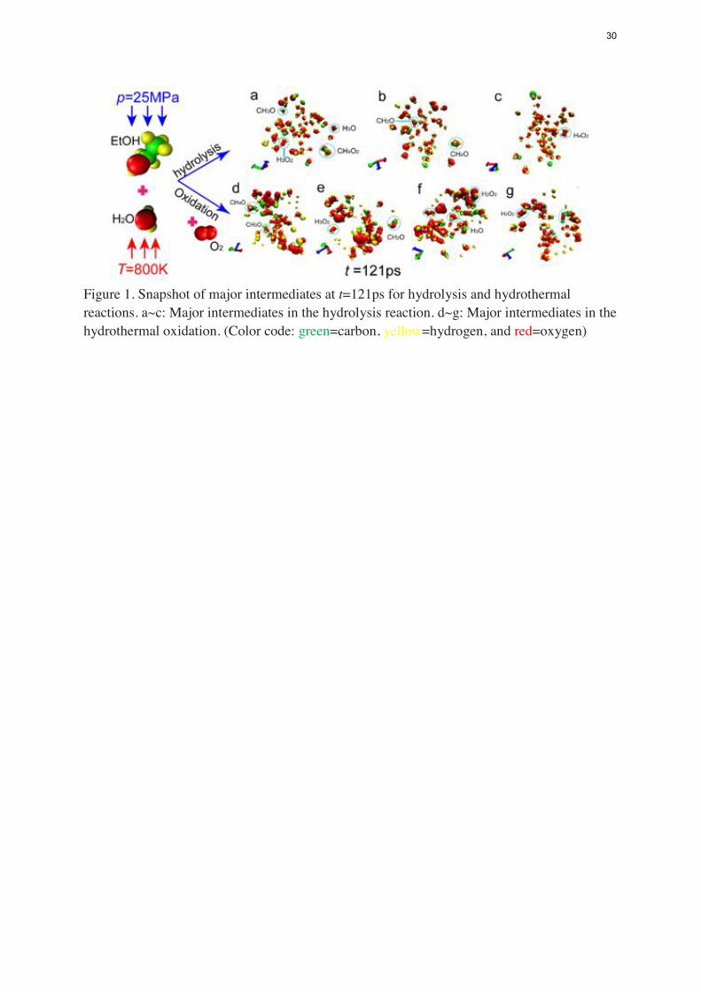
Figure 1. Snapshot of major intermediates at t=121ps for hydrolysis and hydrothermal reactions. a~c: Major intermediates in the hydrolysis reaction. d~g: Major intermediates in the hydrothermal oxidation. (Color code: green=carbon, yellow=hydrogen, and red=oxygen)

30

Assessment of algebraic Flame Surface Density closures in the context of Large Eddy Simulations for head-on quenching of

turbulent premixed flames with non-unity Lewis number Jiawei Lai1 , Nilanjan Chakraborty1, Markus Klein2

1School of Mechanical and System Engineering, Newcastle University, Claremont Road, Newcastle Upon Tyne, NE1 7RU, UK

2Universität der Bundeswehr München, Neubiberg, Germany Introduction

Flame surface density (FSD) based modelling is one of the most well-established reaction rate closures for turbu-lent premixed combustion in the context of Reynolds aver-aged Navier-Stokes (RANS) [1-5] and Large Eddy Simu-lations (LES) [6-12]. Most existing FSD based closures have been proposed for flows without walls, and relatively limited work has been directed to the FSD based closures for flame-wall interaction (FWI) both in the context of RANS [2,3,13] and LES [14]. The generalised FSD Σ𝑔𝑒𝑛 is defined as: Σ𝑔𝑒𝑛 = |∇𝑐| [15], where c is the reaction pro-gress variable, and the overbar indicates LES filtering op-eration. The filtered reaction-diffusion imbalance of c in the context of LES can be closed as: �� + ∇ ⋅ (𝜌𝐷𝑐∇𝑐) =(𝜌𝑆𝐷)𝑠 Σ𝑔𝑒𝑛 where ��, 𝜌 and 𝐷𝑐 are chemical reaction rate, density and progress variable diffusivity respectively. The displacement speed of the 𝑐 = 𝑐∗ isosurface is defined as: 𝑆𝐷 = [�� + ∇ ⋅ (𝜌𝐷𝑐∇𝑐)] 𝜌|∇𝑐||𝑐=𝑐∗⁄ . The quantities �� =𝜌𝑞 /�� and (𝑞)

𝑠 = 𝑞|∇𝑐| |∇𝑐| ⁄ indicate the Favre-filtered and surface-weighted filtered values of a general quantity q, respectively. The effects of 𝐿𝑒 on the algebraic FSD clo-sures in the near-wall region have not yet been analysed, and the present analysis will address this gap in existing literature by explicitly filtering three-dimensional DNS data of head-on quenching of statistically planar turbulent premixed flames with 𝐿𝑒=0.8, 1.0 and 1.2.

Mathematical and Numerical background The algebraic FSD closure proposed by Fureby [8],

once modified to account for resolved scale wrinkling, pro-vides satisfactory performance in the context of LES [11,12]. The modified algebraic FSD closure by Fureby [8] is given by [11]: Σ𝑔𝑒𝑛 = [1 + Γ(𝑢Δ

′ 𝑆𝐿⁄ )]𝐷−2|∇𝑐| (hence-forth referred to as the FUREBY model), where the fractal dimension is expressed in terms of sub-grid scale velocity fluctuation 𝑢Δ

′ = √2𝑘/3 and unstrained laminar burning velocity 𝑆𝐿 as: D=(2.05) (𝑢Δ

′ 𝑆𝐿⁄ + 1) + (2.35) (𝑆𝐿/𝑢Δ′ + 1)⁄⁄ with k being

the sub-grid scale turbulent kinetic energy. The efficiency function for the FUREBY model is expressed as: Γ =0.75 exp[−1.2 (𝑢Δ

′ 𝑆𝐿⁄ )0.3⁄ ] (Δ 𝛿𝐿⁄ )2/3, and 𝛿𝐿 = 𝐷𝑐 𝑆𝐿⁄ is the Zel’dovich flame thickness. An algebraic closure pro-posed by Keppeler et al. [10] which was subsequently used for LES of FWI [14] is given as: Σ𝑔𝑒𝑛 =

* Corresponding author: j.lai@newcastle.ac.uk

𝐶𝑅[2.2Δ max(𝛿𝐿𝐾𝑎Δ−1 2⁄ , 2𝛿𝐿)⁄ ]

𝐷−2 ��(1 − ��)|∇��|𝐹(��)−1 (henceforth referred to as the KEPPELER model), where 𝐹(𝑐) = exp (−[𝑒𝑟𝑓𝑐−1(2(1 − ��))]2), 𝐶𝑅 = 4.5 and 𝐾𝑎Δ = (𝑢Δ

′ 𝑆𝐿⁄ )1.5(Δ 𝛿𝐿⁄ )−0.5 is the sub-grid Karlovitz number and ∆ is the LES filter width. The fractal dimension D in the KEPPELER model is expressed as: 𝐷 =(8/3𝐾𝑎Δ + 0.06) (𝐾𝑎Δ + 0.03)⁄ . The performances of the aforementioned models will be assessed based on ex-plicitly filtered DNS data with 𝐿𝑒 = 0.8, 1.0 and 1.2

Case 𝑢′/𝑆𝐿 𝑙/𝛿𝑡ℎ Da Ka A 5.0 1.67 0.33 8.65 B 6.25 1.44 0.23 13.0 C 7.5 2.5 0.33 13.0 D 9.0 4.31 0.48 13.0 E 11.25 3.75 0.33 19.5

Table 1: Initial values of the simulation parameters for each Le.

A well-known three-dimensional compressible DNS code SENGA [5, 9, 12] has been used to simulate head-on quenching of statistically planar turbulent premixed flames (See Fig. 1) and this DNS data has been used for the as-sessment of algebraic FSD closures for LES. A single step chemistry is used for the purpose of computational econ-omy. The simulation domain is taken to be a rectangular boxe of 70.6𝛿𝐿 × 35.2𝛿𝐿 × 35.2𝛿𝐿, which is discretised by a uniform Cartesian mesh of size 512 × 256 × 256, en-suring at least 10 grid points across the thermal flame thick-ness 𝛿𝑡ℎ = (𝑇𝑎𝑑 − 𝑇0) max|∇��|

𝐿⁄ , where 𝑇𝑎𝑑 , 𝑇0 and ��

are adiabatic, fresh gas and instantaneous temperature re-spectively, and the sub-script 𝐿 denotes the steady un-strained planar laminar flame values. Furthermore, this res-olution ensures that normalised grid size 𝜌0𝑢𝜏∆𝑥/𝜇0 re-mains smaller than unity, where 𝑢𝜏 and 𝜇0 are the friction velocity and unburned gas viscosity, respectively. A no-slip isothermal inert wall with temperature 𝑇𝑤 = 𝑇0, and zero wall-normal mass flux is specified at 𝑥1 = 0, whereas partially non-reflecting outlet boundary condition is speci-fied for the boundary opposite to the isothermal wall. The transverse directions are taken to be periodic. The initial values of normalised turbulent root-mean-square velocity fluctuation 𝑢′ 𝑆𝐿⁄ , integral length scale to thermal flame thickness ratio 𝑙 𝛿𝑡ℎ⁄ , Damköhler number 𝐷𝑎 = 𝑙𝑆𝐿 𝛿𝑡ℎ𝑢′⁄

31

and Karlovitz number 𝐾𝑎 = (𝑢′ 𝑆𝐿⁄ )3 2⁄ (𝑙 𝛿𝑡ℎ⁄ )−1 2⁄ away from the wall are shown in Table 1. The heat release pa-rameter 𝜏 = (𝑇𝑎𝑑 − 𝑇0)/𝑇0 and Zel’dovich number 𝛽 are taken to be 6.0 for all cases considered here.

Figure 1: Instantaneous views of c and T: 𝑡1 = 2.1𝛿𝐿/𝑆𝐿 and 𝑡2 = 6.3𝛿𝐿/𝑆𝐿 for turbulent case E.

Figure 2: Variation of < (𝜌 𝑆𝐷)𝑠 𝛴𝑔𝑒𝑛 > with 𝑥1/𝛿𝐿 : DNS

data ——, FUREBY model —— KEPPLER model ——, broken line indicates original FSD model <(𝜌 𝑆𝐷)𝑠 𝛴𝑔𝑒𝑛 >, * indicates < (𝜌 𝑆𝐷)𝑠

𝛴𝑔𝑒𝑛𝑄𝐴 >, o indi-cates < (𝜌 𝑆𝐷)𝑠

𝛴𝑔𝑒𝑛𝑄𝐵 > for case C.

Results & Discussion The distributions of non-dimensional temperature 𝑇 =

(𝑇 − 𝑇0)/(𝑇𝑎𝑑 − 𝑇0) and reaction progress variable c are shown in Fig. 1 at different time instants for flames with 𝐿𝑒 = 0.8, 1.0 and 1.2 to give an idea about the flow do-main. The variation of < (𝜌 𝑆𝐷)𝑠

Σ𝑔𝑒𝑛 > with the normal-ised wall normal distance 𝑥1/𝛿𝐿 for case C is shown in Fig. 2, where of < 𝑞 > represents the value of q averaged over statistically homogeneous directions. The quantity |∇𝑐| is evaluated based on equivalent LES grid for the results shown in Fig. 2. The predictions of < (𝜌 𝑆𝐷)𝑠

Σ𝑔𝑒𝑛 > ac-cording to the FUREBY and KEPPELER models are also shown in Fig. 2 along with the predictions with near-wall

damping functions (i.e. < (𝜌 𝑆𝐷)𝑠 Σ𝑔𝑒𝑛𝑄𝐴 > and <

(𝜌 𝑆𝐷)𝑠 Σ𝑔𝑒𝑛𝑄𝐵 >), where 𝑄𝐴 = [1 + 48(��𝑤 −

��𝑤)]𝑒𝑥𝑝 {−𝛽 [𝜏(�� − ��) ((1 + 𝜏��)(1 + 𝜏��))⁄ ]0.25

} [3] and 𝑄𝐵 =exp[−2.0𝛽(�� − ��)] [2] are the damping factors according to Alshaalan and Rutland [3] and Bruneaux et al. [2] re-spectively. These damping factors are supposed to account for the reduced extent of flame wrinkling and burning rate due to flame quenching in the near-wall region. For sΔ ≤𝛿𝑡ℎ, both the FUREBY and KEPPELER models in their original form and with damping function 𝑄𝐵 satisfactorily predict < (𝜌 𝑆𝐷)𝑠

Σ𝑔𝑒𝑛 > extracted from DNS data when the flame is away from the wall. Slight under-prediction occurs for all models except FUREBY model for 𝐿𝑒 ≠ 1.0 flames. The prediction of < (𝜌 𝑆𝐷)𝑠

Σ𝑔𝑒𝑛𝑄𝐵 > according to the FUREBY model shows a satisfactory level of agree-ment with DNS data for Δ ≤ 2.0𝛿𝑡ℎ but this model shows under-prediction for Δ > 2.0𝛿𝑡ℎ. For all models, an under-prediction of < (𝜌 𝑆𝐷)𝑠

Σ𝑔𝑒𝑛 > has been obtained in the near wall region.

Conclusions The performances of algebraic FSD closures in the case

of head-on quenching of statistically planar premixed tur-bulent flames with different 𝐿𝑒 have been assessed based on a priori DNS analysis.

Acknowledgements The authors are grateful to N8 and ARCHER for the

computational support.

References [1] R.S. Cant, S.B. Pope and K.N.C. Bray, Proc. Combust.

Inst. 27 (1990) 809-815. [2] G. Bruneaux, T. Poinsot, J. H. Ferziger, J. Fluid Mech.

349 (1997) 191-219. [3] T. Alshaalan, C. J. Rutland, Proc. Combust. Inst. 27

(1998) 793-799. [4] I. Han, K.Y. Huh, Combust. Flame 152 (2008) 194-

205. [5] N. Chakraborty, R. S. Cant, Combust. Flame 158

(2011) 1768-1787. [6] M. Boger, D. Veynante, H. Boughanem and A.Trouvé,

Proc. Combust. Inst. 27 (1998) 917-925. [7] E.R. Hawkes, R.S. Cant, Combust. Flame 126 (2001)

1617-1629. [8] C. Fureby, Proc. Combust. Inst. 30 (2005) 593-601. [9] N. Chakraborty, M. Klein, Phys. Fluids, 20 (2008)

085108. [10] R. Keppeler, E. Tangermann, U. Allaudin, M. Pfitzner,

Flow Turb. Combust. 97 (2014) 767-802. [11] T. Ma, O. Stein, N. Chakraborty, A. Kempf, Combust.

Theor. Modell. 17 (2013) 431-482. [12] M. Klein, N. Chakraborty, M. Pfitzner, Flow Turb.

Combust. (2016) accepted. [13] T.J. Poinsot, D.C. Haworth, G. Bruneaux, Combust.

Flame 95 (1993) 118-132. [14] R. Keppeler, M. Pfitzner, L.T.W. Chong, T. Komarek,

W., Polifke, ASME Turbo Expo, 2 (2012) 457-467. [15] M. Boger, D. Veynante, H. Boughanem, A. Trouve,

Proc. Comb. Ins. 27 (1998) 917-925.

32

Investigation of Flame-Wall Interaction with Rough-Wall: A DNS Study

Y. X, Yang * , K.K.J. Ranga Dinesh Energy Technology Research Group, Faculty of Engineering and the Environment,

University of Southampton, UK

(Corresponding author: yxy1a14@soton.ac.uk)

Abstract Understanding the interactions of flames with walls is an important process in designing modern combustion devices [1]. In this paper, two-dimensional direct numerical simulation (DNS) with detailed chemistry has been carried to study the flame-wall interaction effect in the presence of wall roughness. Instead of some complicated techniques to mathematically model the rough wall boundary, a simple forcing approach is adopted to describe the roughness effects on the turbulence-flame interactions in the near-wall region. The roughness effect has been numerically produced by adding an external forcing terms into the momentum and energy equations. Due to the roughness effect in the near-wall flow-field, the flame characteristics are in turn influenced. The full paper will present the comparison of flow field and flame characteristics between the smooth and the rough wall cases. Forcing approach of wall roughness in chemically reacting flow: In this work, we study the wall roughness effects by using the approach developed by Busse and Sandham [2]. Besides the roughness term in the momentum equations, the external drag effect on energy conservation has been included.

∂ρu𝑖∂t

+∂𝐅𝑗∂x𝑗

=∂𝐅𝑗,𝑣𝑖𝑠∂x𝑗

+ 𝑓𝑟𝑖

𝑓𝑟𝑖 = −α𝑖ρF(h𝑖)u𝑖|u𝑖| ∂E∂t

+∂𝐅𝑗∂x𝑗

=∂𝐅𝑗,𝑣𝑖𝑠∂x𝑗

+ u𝑗𝑓𝑟𝑗

Note i denotes each direction and j apply for summation convention. And α is roughness line density [L-1]. Roughness height is modelled using height function F(h). Problem configuration: 2D DNS Calculations are performed using the code parcomb [3] with a reacting channel flow with 10mm in length and 3mm in height (Fig.1). Navier-Stokes Characteristics Boundary Conditions (NSCBC) are used in simulation, with left and right boundaries are periodic, while both top and bottom wall are set to be isothermal with a constant temperature 450K. A spherical syngas flame kernel with radius 1mm is initialized at near the left boundary.

Fig. 1. 2D problem configuration

33

Roughness effect on the reacting flow: Figure 2 shows that the wall roughness decreases the flow velocity near the wall and make the flame evolution near the wall more sluggish, differing from the smooth case.

Fig.2. Comparison of velocity filed of the computational domain, (a) smooth case, (b) rough

case. Figure 3 shows the roughness term distribution. As seen from Fig. 3, one can see that the roughness-like drag mainly functions against the flame kernel.

Fig. 3. Contours of roughness term in the x-direction momentum equation

References: [1]. A. Gruber, R. Sankaran, E. H. Hawkes, J. H. Chen. Turbulent flame-wall interaction: a direct numerical simulation study. J. Fluid Mech. (2010), vol. 658, pp.5-32. [2]. A. Busse, N. D. Sandham. Parametric forcing approach to rough-wall turbulent channel flow. J. of Fluid Mech. (2012), vol. 712, pp.169-202. [3]. R. Hilbert, F. Tap, H. El-Rabii, D. Thevenin. Impact of detailed chemistry and transport models on turbulent combustion simulations Prog. Energy Combust. Sci. (2004), vol. 30, pp. 165–193.

(a)

(b)

34

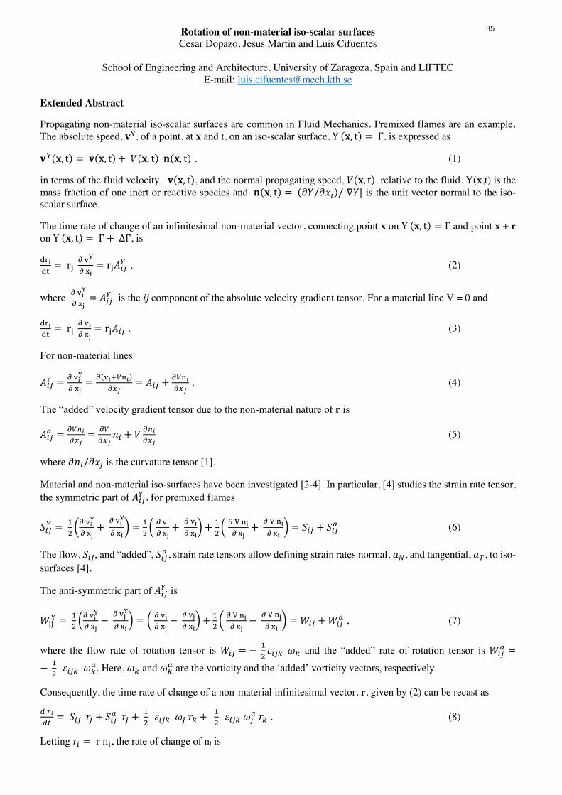
Rotation of non-material iso-scalar surfaces Cesar Dopazo, Jesus Martin and Luis Cifuentes

School of Engineering and Architecture, University of Zaragoza, Spain and LIFTEC E-mail: luis.cifuentes@mech.kth.se

Extended Abstract

Propagating non-material iso-scalar surfaces are common in Fluid Mechanics. Premixed flames are an example. The absolute speed, 𝐯Y, of a point, at x and t, on an iso-scalar surface, Y (𝐱, t) = Γ, is expressed as

𝐯Y(𝐱, t) = 𝐯(𝐱, t) + 𝑉(𝐱, t) 𝐧(𝐱, t) , (1)

in terms of the fluid velocity, 𝐯(𝐱, t), and the normal propagating speed, 𝑉(𝐱, t), relative to the fluid. Y(x,t) is the mass fraction of one inert or reactive species and 𝐧(𝐱, t) = (𝜕𝑌/𝜕𝑥𝑖)/|∇𝑌| is the unit vector normal to the iso-scalar surface.

The time rate of change of an infinitesimal non-material vector, connecting point x on Y (𝐱, t) = Γ and point x + r on Y (𝐱, t) = Γ + ΔΓ, is

dridt = rj ∂ vi

Y

∂ xj= rj𝐴𝑖𝑗

𝑌 , (2)

where ∂ viY

∂ xj= 𝐴𝑖𝑗

𝑌 is the ij component of the absolute velocity gradient tensor. For a material line V = 0 and

dridt = rj ∂ v𝑖

∂ xj= rj𝐴𝑖𝑗 . (3)

For non-material lines

𝐴𝑖𝑗𝑌 = ∂ vi

Y

∂ xj= 𝜕(v𝑖+𝑉𝑛𝑖)

𝜕𝑥𝑗= 𝐴𝑖𝑗 + 𝜕𝑉𝑛𝑖

𝜕𝑥𝑗 . (4)

The “added” velocity gradient tensor due to the non-material nature of r is

𝐴𝑖𝑗𝑎 = 𝜕𝑉𝑛𝑖

𝜕𝑥𝑗= 𝜕𝑉

𝜕𝑥𝑗𝑛𝑖 + 𝑉 𝜕𝑛𝑖

𝜕𝑥𝑗 (5)

where 𝜕𝑛𝑖/𝜕𝑥𝑗 is the curvature tensor [1].

Material and non-material iso-surfaces have been investigated [2-4]. In particular, [4] studies the strain rate tensor, the symmetric part of 𝐴𝑖𝑗

𝑌 , for premixed flames

𝑆𝑖𝑗𝑌 = 1

2 (∂ viY

∂ xj+ ∂ vj

Y

∂ xi) = 12 ( ∂ vi

∂ xj+ ∂ vj

∂ xi) + 1

2 ( ∂ V ni∂ xj

+ ∂ V nj∂ xi

) = 𝑆𝑖𝑗 + 𝑆𝑖𝑗𝑎 (6)

The flow, 𝑆𝑖𝑗, and “added”, 𝑆𝑖𝑗𝑎 , strain rate tensors allow defining strain rates normal, 𝑎𝑁, and tangential, 𝑎𝑇, to iso-

surfaces [4].

The anti-symmetric part of 𝐴𝑖𝑗𝑌 is

𝑊ijY = 1

2 (∂ viY

∂ xj− ∂ vj

Y

∂ xi) = ( ∂ vi

∂ xj− ∂ vj

∂ xi) + 1

2 ( ∂ V ni∂ xj

− ∂ V nj∂ xi

) = 𝑊𝑖𝑗 + 𝑊𝑖𝑗𝑎 , (7)

where the flow rate of rotation tensor is 𝑊𝑖𝑗 = − 12 𝜀𝑖𝑗𝑘 𝜔𝑘 and the “added” rate of rotation tensor is 𝑊𝑖𝑗

𝑎 =− 1

2 𝜀𝑖𝑗𝑘 𝜔𝑘𝑎. Here, 𝜔𝑘 and 𝜔𝑘

𝑎 are the vorticity and the ‘added’ vorticity vectors, respectively.

Consequently, the time rate of change of a non-material infinitesimal vector, r, given by (2) can be recast as

𝑑 𝑟𝑖𝑑𝑡 = 𝑆𝑖𝑗 𝑟𝑗 + 𝑆𝑖𝑗

𝑎 𝑟𝑗 + 12 𝜀𝑖𝑗𝑘 𝜔𝑗 𝑟𝑘 + 1

2 𝜀𝑖𝑗𝑘 𝜔𝑗𝑎 𝑟𝑘 . (8)

Letting 𝑟𝑖 = r ni, the rate of change of ni is

35

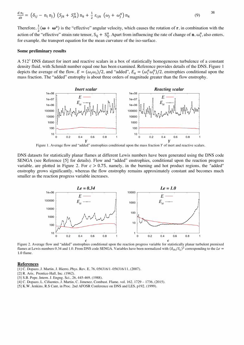
𝑑 n𝑖𝑑𝑡 = (𝛿𝑖𝑗 − n𝑖 n𝑗) (𝑆𝑗𝑘 + 𝑆𝑗𝑘

𝑎 ) n𝑘 + 12 𝜀𝑖𝑗𝑘 (𝜔𝑗 + 𝜔𝑗

𝑎) n𝑘 (9) Therefore, 1

2 (𝛚 + 𝛚a) is the “effective” angular velocity, which causes the rotation of r, in combination with the action of the “effective” strain rate tensor, Sij + Sij

a. Apart from influencing the rate of change of n, ωia, also enters,

for example, the transport equation for the mean curvature of the iso-surface. Some preliminary results A 5123 DNS dataset for inert and reactive scalars in a box of statistically homogeneous turbulence of a constant density fluid, with Schmidt number equal one has been examined. Reference provides details of the DNS. Figure 1 depicts the average of the flow, 𝐸 = (𝜔𝑖𝜔𝑖)/2, and “added”, 𝐸𝑎 = (𝜔𝑖

𝑎𝜔𝑖𝑎)/2, enstrophies conditional upon the

mass fraction. The “added” enstrophy is about three orders of magnitude greater than the flow enstrophy.

Figure 1. Average flow and “added” enstrophies conditional upon the mass fraction 𝑌 of inert and reactive scalars.

DNS datasets for statistically planar flames at different Lewis numbers have been generated using the DNS code SENGA (see Reference [5] for details). Flow and “added” enstrophies, conditional upon the reaction progress variable, are plotted in Figure 2. For 𝑐 > 0.75, namely, in the burning and hot product regions, the "added" enstrophy grows significantly, whereas the flow enstrophy remains approximately constant and becomes much smaller as the reaction progress variable increases.

Figure 2. Average flow and “added” enstrophies conditional upon the reaction progress variable for statistically planar turbulent premixed flames at Lewis numbers 0.34 and 1.0. From DNS code SENGA. Variables have been normalized with (𝛿𝑡ℎ/𝑆𝐿)2 corresponding to the 𝐿𝑒 =1.0 flame.

References [1] C. Dopazo, J. Martin, J. Hierro, Phys. Rev. E, 76, 056316/1–056316/11, (2007). [2] R. Aris, Prentice-Hall, Inc. (1962). [3] S.B. Pope, Intern. J. Engng. Sci., 26, 445-469, (1988). [4] C. Dopazo, L. Cifuentes, J. Martin, C. Jimenez, Combust. Flame, vol. 162, 1729 – 1736, (2015). [5] K.W. Jenkins, R.S Cant, in Proc. 2nd AFOSR Conference on DNS and LES, p192, (1999).

36

Analysis of Turbulent Flame Propagation in Equivalence Ratio-Stratified Flow

Edward S. Richardsona1and Jacqueline H. Chen2

1Faculty of Engineering and the Environment, University of Southampton, Southampton, SO17 1BJ, UK

2Combustion Research Facility, Sandia National Laboratories, Livermore, CA 94551-0969, USA

Equivalence ratio-stratified combustion is an important technology for achieving stable low-emission operation in internal combustion engines and gas turbines. This study examines how equivalence ratio stratification affects the physics of turbulent flame propagation using Direct Numerical Simulation. Three-dimensional simulations of a turbulent slot-Bunsen flame configuration are performed with accurate multi-step kinetic modelling for methane-air combustion, illustrated in Fig. 1. We compare one perfectly-premixed and three equivalence ratio-stratified cases with the mean equivalence ratio gradient aligned with, tangential to or opposed to the mean flame brush.

Figure 1. Volume rendering of the instantaneous heat-release field coloured by mixture fraction for case C2. Turbulent premixed combustion in the flamelet regime involves a propagating flame surface which is distorted by its interactions with the turbulent flow. According to this description, the turbulent flame speed of a homogeneous mixture, 𝑆𝑇, will differ from the laminar flame speed 𝑆𝐿, according to,

𝑆𝑇⟨𝑆𝐿⟩𝑠

= 𝐼0𝐴′ (1)

where 𝐴′ is the ratio of the turbulent flame area 𝐴𝑡𝑢𝑟𝑏. divided by the projected frontal area of the flame, A,

𝐴′ = 𝐴𝑡𝑢𝑟𝑏.

𝐴 , (2)

and the burning intensity 𝐼0 is the ratio of the surface averaged displacement speed to the surface-averaged laminar flame speed, ⟨𝑆𝐿⟩𝑠 . The laminar flame speed is surface-averaged in this presentation because, in

a e.s.richardson@soton.ac.uk

37

equivalence ratio-stratified flows, 𝑆𝐿 varies depending on the local value of the equivalence ratio, 𝜑(𝒙). Application of Eq. 1 to stratified combustion raises two distinct questions: first, how does stratification influence the flame surface area in a turbulent flame; and second, how does stratification influence the burning intensity? The objective of this study is to address both of these questions by examining DNS data for turbulent stratified combustion with realistic methane-air chemistry. The simulation results are analysed in terms of flame surface area and the burning intensity. The local effects of stratification are then investigated further by examining statistics of the displacement speed conditioned on the flame-normal equivalence ratio gradient. The local burning intensity is found to depend on the orientation of the stratification with respect to the flame front, so that burning intensity is enhanced when the flame speed in the products is faster than in the reactants. This effect of alignment between equivalence ratio gradients and flame fronts has been observed previously in laminar flames [1] and related effects have been observed in laboratory measurements for turbulent flames [2], and it is found here that it also affects the global behaviour of turbulent flames. The flame surface area is also influenced by equivalence ratio stratification and this may be explained by differences in the surface-averaged consumption speed and differential propagation effects due to flame speed variations associated with equivalence ratio fluctuations.

Figure 2. Conditionally-averaged displacement speed versus flame-normal mixture fraction gradient. Circles: case C2 at 𝑥/𝐿𝑥 = 0.5; Triangles: laminar counter-flow flame data. Flame surface area generation by differential propagation is expected to be relatively limited in the current DNS due the high turbulence intensity. The stratification however has a significant influence on the flame surface area due to the variation of the flame surface averaged consumption speed with surface averaged equivalence ratio and equivalence ratio gradient orientation. The differential propagation mechanism however promotes a preferential alignment of the local equivalence ratio gradient with the flame front that depends on the local equivalence ratio. This effect contributes to the average burning intensity and, as a consequence, may feed back to the overall flame surface generation. There is now a need for further analysis of the scaling of front/back-support and differential propagation effects in order to delineate regimes of equivalence ratio-stratified combustion where these effects are significant and may require modelling. References [1] E.S. Richardson, V.E. Granet, A. Eyssartier, J.H. Chen, Combust. Theor, Model. 14 (6) (2010)

775-792. [2] M.S. Sweeney, S. Hochgreb, M.J. Dunn, R.S. Barlow, Combust. Flame 160 (2013) 322–334.

38

Influence of pressure Hessian on flame turbulence interaction inpremixed combustion

Umair Ahmed1⇤, Malgorzata Zimon1, Girish Nivarti2, Robert Prosser1 and Robert Stewart Cant21School of MACE, University of Manchester, Manchester M13 9PL, UK.2Department of Engineering, University of Cambridge, Cambridge CB2 1PZ, UK.

Introduction

The behaviour of the mean reaction rate in premixed turbulent combustion is strongly dependent on the scalar dis-sipation rate (ee

c

). Across a range of characteristic Damköhler numbers, the effect of the turbulent flow field on thetransport of ee

c

is dominated by Flame Turbulence Interaction (FTI) – denoted here by eDc

[1, 2]. This quantity ap-

pears explicitly in the transport equation for scalar dissipation and has the form✓

reDc

⌘ ra g∂c

00

∂x

i

S

00i j

∂c

00

∂x

j

◆. In flames

of engineering interest, the behaviour of eDc

depends on the alignment between the scalar gradient and the principaldirections of the hydrodynamic strain rate [3]. In cold-flow turbulence �reD

c

is a net source term for eec

arising fromthe strong statistical alignment between scalar gradient and principal compressive strain rate eigenvector [4, 5]. Bycontrast, in flows with intense heat release, the scalar gradient preferentially aligns with the principal extensive strainrate eigenvector, making �reD

c

a net sink term for eec

[6].In order to understand this phenomena accurately a transport equation for eD

c

has been developed by Ahmed et al[7, 8]; this has established that the behaviour of eD

c

is principally determined by the competition between reaction rategradients and the pressure Hessian on the one hand, and diffusion and dissipation on the other. It has been established

in earlier studies that one of the key parameters that controls eDc

is the pressure Hessian term✓

a ∂c

00

∂x

i

∂ 2p

0

∂x

i

∂x

j

∂c

00

∂x

j

= f◆

.

In the case of cold flows Suman and Girimaji [9] have shown that the pressure Hessian changes alignment with thestrain field across regions of high compressibility (i.e. shock waves), but no work has been undertaken to study thebehaviour of the pressure Hessian in density stratified flows with or without heat release. In this work we study thebehaviour of the pressure Hessian in premixed flames subjected to high levels of turbulence.

Direct Numerical Simulations

The Direct Numerical Simulations (DNS) used in this study are representative of lean, unit Lewis number flames.The chemical kinetics are approximated by the single step reaction R ! P. DNS of planar flames was carried out usingthe code called SENGA2, in which the conservation equations for mass, momentum, energy and reacting species aresolved for compressible flow [10]. Navier-Stokes Characteristic Boundary Conditions (NSCBC) have been applied toall non-periodic boundaries. The domain size for these simulations is L

x

/3= L

y

= L

z

= 13.89d 0L

, where d 0L

is the flamethermal thickness. The domain is discretised by a 288⇥ 96⇥ 96 node uniform grid, ensuring a minimum resolutionof about 10 grid points is maintained to resolve the laminar flame thermal thickness. The global thermochemicalparameters used in the simulations are unstretched laminar flame speed u

0L

= 0.39 m/s; d 0L

= 0.36 mm; heat releaseparameter t = 6.66 and the Zeldovich number b = 6.0. The flames studied in this work lie in the thin reaction zoneregime on the Borghi diagram. Further details for the DNS can be found in [11].

Results

Figure 1a shows the pressure Hessian term f . The signal is very noisy and it is not easy to separate the true behaviourof the term from the noise. These high frequency oscillations occur in the pressure field due to the shortfalls of thestandard NSCBC approach used at the non-periodic boundaries in the current simulations [12]. To estimate the correctbehaviour of the pressure Hessian term the data is filtered by using a novel filtering approach, which combines thestrengths of singular spectrum analysis (SSA) [13, 14] and wavelet thersholding [15, 16]. The filtered term can be seenin figure 1b. The pressure Hessian term is now seen as a source for eD

c

at the leading edge of the flame, becoming a sinkterm towards the trailing edge of the flame. To investigate this further we study the alignment of the pressure Hessianeigenvectors with the scalar gradient as shown in figure 2. It can be seen that the extensive part of the pressure Hessianeigenvector aligns with the flame gradients in the regions of intense heat release. Further results and discussion are

⇤corresponding author: umair.ahmed@manchester.ac.uk

1

39

going to form part of the oral presentation.

!c

0 0.2 0.4 0.6 0.8 1

φ-150

-100

-50

0

50

100

150

200

(a) original f

!c

0 0.2 0.4 0.6 0.8 1

φ

-60

-40

-20

0

20

40

60

80

100

(b) filtered f

Figure 1: f profile across the flame in case C. The values are normalised using the respective r0, u

0L

and d 0L

.

|cosθf1 |0 0.5 1

p(|cosθ

f1|)

1

1.1

1.2

1.3

1.4

1.5

1.6c=0.1c=0.3c=0.5c=0.7c=0.8

(a) Direction cosine between f1 and —c

|cosθf2 |0 0.5 1

p(|cosθ

f2|)

0.8

0.9

1

1.1

1.2

1.3

1.4

1.5c=0.1c=0.3c=0.5c=0.7c=0.8

(b) Direction cosine between f2 and —c

|cosθf3 |0 0.5 1

p(|cosθ

f3|)

1

1.1

1.2

1.3

1.4

1.5

1.6c=0.1c=0.3c=0.5c=0.7c=0.8

(c) Direction cosine between f3 and —c

Figure 2: Pdfs of the direction cosines. Where f1, f2 and f3 are the extensive, intermediate and compressive eigen-vectors of ∂ 2

p

∂x

i

∂x

j

.

References

[1] Swaminathan, N. and Grout, R. W., “Interaction of turbulence and scalar fields in premixed flames,” Physics of Fluids, Vol. 18,No. August 2005, 2006, pp. 1–9.

[2] Swaminathan, N. and Bray, K. N. C., “Effect of dilatation on scalar dissipation in turbulent premixed flames,” Combustion

and Flame, Vol. 143, No. 4, dec 2005, pp. 549–565.[3] Kolla, H., Rogerson, J. W., Chakraborty, N., and Swaminathan, N., “Scalar dissipation rate modeling and its validation,”

Combustion Science and Technology, Vol. 181, No. 3, feb 2009, pp. 518–535.[4] Ashurst, W. T., Kerstein, A. R., Kerr, R. M., and Gibson, C. H., “Alignment of vorticity and scalar gradient with strain rate in

simulated Navier Stokes turbulence,” Physics of Fluids, Vol. 30, No. 8, 1987, pp. 2343.[5] Batchelor, G., “The effect of homogeneous turbulence on material lines and surfaces,” Proceedings of the Royal Society of

London. Series A, Mathematical and Physical Sciences, Vol. 213, No. 1114, 1952, pp. 349–366.[6] Chakraborty, N. and Swaminathan, N., “Influence of the Damköhler number on turbulence-scalar interaction in premixed

flames. I. Physical insight,” Physics of Fluids, Vol. 19, No. 4, 2007, pp. 045103.[7] Ahmed, U., Prosser, R., and Revell, A. J., “Towards the development of an evolution equation for flame turbulence interaction

in premixed turbulent combustion,” Flow, Turbulence and Combustion, Vol. 93, No. 4, 2014, pp. 637–663.[8] Ahmed, U. and Prosser, R., “Modelling flame turbulence interaction in RANS simulation of premixed turbulent combustion,”

Combustion Theory and Modelling, Vol. 20, No. 1, jan 2016, pp. 34–57.[9] Suman, S. and Girimaji, S. S., “Velocity gradient dynamics in compressible turbulence: Characterization of pressure-Hessian

tensor,” Physics of Fluids, Vol. 25, No. 12, 2013, pp. 125103.[10] Cant, R. S., “SENGA2 User Guide, CUED/ A-THERMO/TR67,” Tech. rep., University of Cambridge, Cambridge, United

Kingdom, 2012.[11] Nivarti, G. V. and Cant, R. S., “Aerodynamic Quenching and Burning Velocity of Turbulent Premixed Methane-Air Flames,”

Proceedings of ASME Turbo Expo 2015: Turbine Technical Conference and Exposition. Volume 4B: Combustion, Fuels and

Emissions, ASME, jun 2015.[12] Prosser, R., “Improved boundary conditions for the DNS of reacting subsonic flows,” Flow, Turbulence and Combustion,

Vol. 87, No. 2-3, oct 2010, pp. 351–376.[13] Golyandina, N., Nekrutkin, V., and Zhigljavsky, A., Analysis of Time Series Structure: SSA and Related Techniques, CRC

Press, 2010.[14] Golyandina, N. and Zhigljavsky, A., Singular Spectrum Analysis for Time Series, Springer, 2013.[15] Donoho, D. L. and Johnstone, J. M., “Ideal spatial adaptation by wavelet shrinkage,” Biometrika, Vol. 81, No. 3, 1994,

pp. 425–455.[16] Mallat, S. G., A wavelet Tour of Signal Processing, Academic Press, 1999.

2

40

Formation of Nascent Soot Clusters from Polycyclic Aromatic Hydrocarbons: A ReaxFF Molecular Dynamics Study

Qian Mao1, Adri C.T. van Duin2, K. H. Luo 1,3*

1Center for Combustion Energy, Key Laboratory for Thermal Science and Power Engineering of Ministry of Education, Department of Thermal Engineering, Tsinghua University, Beijing 100084, China 2Department of Mechanical and Nuclear Engineering, The Pennsylvania State University, University Park, PA 16802, USA 3Department of Mechanical Engineering, University College London, Torrington Place, London WC1E 7JE, UK *Email: K.Luo@ucl.ac.uk Abstract The process of nucleation of gas phase polycyclic aromatic hydrocarbon (PAH) molecules to form soot particles involves both chemical reaction and physical processes, which is still poorly understood.1 In the present study, we use ReaxFF molecular dynamics simulations3 to study the physical and chemical processes of soot nucleation from PAHs. Two types of PAHs typically found in a flame enviroment,2 coronene and pyrene, are selected for simulation over a range of temperatures from 400 K to 2000 K, with or without the presence of noble metal clusters or H radicals. Both coronene and pyrene are more likely to coalesce into stacked clusters at low temperatures (e.g. 400 K) due to physical effects. Firstly, PAHs grow into stacking clusters, in parallel to each other. Collisions of these clusters lead to the nascent soot particles. With increasing temperature, some of the coronene PAHs cluster physically to form large particles, while some dissociate into smaller molecules and radicals. At elevated temperature (> 1400K), collisions from the dissociated smaller molecules or radicals and higher kinetic energy of the PAHs causes the nascent soot particles to break up into smaller clusters. This is consistent with previous studies, where the condensed-phase PAHs evaporate, rather than condense into particles at flame temperatures around 1600 K.1

In addition, we found that pyrene PAHs are more difficult to coalesce with the temperature rise since they have weaker binding energy than coronene PAHs. When adding the Ni13 clusters to the PAHs, the nucleation of the PAHs (coronene, pyrene) not only happens in the low temperature region but also at temperatures as high as 2000 K. Specifically, PAHs firstly nucleate around the Ni13 clusters. Then other PAHs join to form a staking structure based on the internal PAHs around the Ni13 clusters. Afterwards, the formed nascent soot clusters may collide to form larger soot particles. It is noteworthy that soot particles formed based on Ni clusters can survive the high temperatures. That is, Ni clusters enhance the binding energy between PAHs. The effect of H radicals on the PAHs nucleation is limited in the low temperature region, as the chemical reaction between H radicals and PAH is highly sensitive to temperature. At high temperatures, H radicals react with PAHs readily. The nucleation between PAHs through the HACA mechanism4 is observed in the simulations, in

41

which a gaseous H radical abstracts a H atom from a PAH, followed by the addition of other PAH to the radical site, leading to a crosslinked soot structure.

Figure 1. Nucleation of Coronenes at 400 K into a soot particle.

References [1] Wang, Hai. "Formation of nascent soot and other condensed-phase materials in flames." Proceedings of the Combustion Institute 33.1 (2011): 41-67. [2] Totton, Tim S., et al. "Modelling the internal structure of nascent soot particles." Combustion and Flame 157.5 (2010): 909-914. [3] Van Duin, Adri CT, et al. "ReaxFF: a reactive force field for hydrocarbons." The Journal of Physical Chemistry A 105.41 (2001): 9396-9409. [4] Frenklach, Michael. "Reaction mechanism of soot formation in flames." Physical Chemistry Chemical Physics 4.11 (2002): 2028-2037.

42

Effect of the SO2 and H2S presence on the formation of PAH and soot during the pyrolysis of ethylene

F. Viteria,b, M. Abiána,c, Á. Milleraa, R. Bilbaoa, M.U. Alzuetaa*

* corresponding author: uxue@unizar.es

aAragón Institute of Engineering Research (I3A), Department of Chemical and Environmental Engineering, University of Zaragoza, Río Ebro Campus, 50018 Zaragoza, Spain.

bFacultad de Ciencias de la Ingeniería, Universidad Tecnológica Equinoccial, Quito-Ecuador cInstituto de Carboquímica (ICB-CSIC), Department of Energy & Environment, Zaragoza 50018, Spain

Introduction Fuels used in combustion processes contain sulphur, which is released to the gas-phase during fuel use, mostly as SO2. Besides the pollutant character of SO2 when is emitted to the atmosphere, SO2 has shown a direct effect on the formation of soot and polycyclic aromatic hydrocarbons (PAH) [1-4]. On the other hand, a very abundant fuel such as sour gas, from which it is obtained elemental sulphur through the Claus process, could be also further used as a fuel without expensive pre-treatments [5], even considering that the main sulphur compound present in this fuel is H2S. Therefore, different studies have been developed in order to better understand the role of these sulphur compounds in the combustion process [6, 7]. However, due to the complexity of the process, there are still issues not fully known. In this context, previous studies by our group have reported that SO2 and H2S act on the soot [1, 8] and PAH [4] formation during the pyrolysis of ethylene. The present study focuses on the comparison of the effect of SO2 and H2S on the pyrolysis of ethylene, analysing their influence on the soot and 16 priority EPA-PAH formation, which are considered by the United States Environmental Protection Agency (US-EPA) as priority pollutants [9]. Methodology The pyrolysis experiments were performed under well-controlled laboratory conditions, in a quartz flow reactor at atmospheric pressure. The reactants consist of SO2, H2S and ethylene, all of them diluted in N2. The concentration of ethylene was fixed on 30000 ppmv, and both SO2 and H2S concentrations were modified at 1475 K, to cover a wide range: 0, 0.3, 0.5 and 1%. In addition, the pyrolysis of either C2H4-1% SO2 and C2H4-1% H2S was studied in the 1075-1475 K temperature range. The outlet gases were analysed by a gas cromatograph, a Fourier Transform Infrared (FTIR) analyser, and a micro-cromatograph. Soot was collected in a glass fiber filter, and the PAH formed were collected and quantified following a method previously developed by our research group [10]. In particular, the EPA-PAH collection was made from different places where these compounds could be present, such as adsorbed on the soot surface (trapped in the soot filter), stuck on the reactor walls, and in the outlet gas and retained by a XAD-2 resin. A fraction of the soot formed during the experiments and the XAD-2 resin, were subjected to Soxhlet extraction with dichloromethane, and concentrated by rotary evaporation. The reactor walls were washed with 150 mL of dichloromethane to trap PAH that could be stuck on the reactor walls. All the samples were analysed by gas chromatography-mass spectrometry (GC/MS). Results Fig. 1a shows the results of soot and PAH obtained both in the pyrolysis of C2H4 and in the pyrolysis of C2H4 in the presence of H2S and SO2 at 1475 K, and as a function of the inlet concentration of the sulphur compound. The presence of sulphur compounds shows a high response to reduce the amounts of soot and EPA-PAH, producing a reduction of soot of 20% for 1% SO2, and 5% for 1% H2S. In relation to the EPA-PAH, the reductions achieved in the presence of either SO2 or H2S are more noticeable than for soot, 59% and 29% of reduction, respectively. It is remarkable that the presence of a reduced species, such as H2S, also acts to suppress soot and EPA-PAH formation. A slight reduction of the formation of soot is obtained when the inlet concentration of H2S is increased, being more noticeable by increasing the concentration of SO2. The same observation can be done for the formation of total EPA-PAH. Fig. 1b shows soot and EPA-PAH obtained in the pyrolysis of the C2H4-sulphur compounds mixtures as a function of temperature. In all the cases, soot formation starts at 1275 K, and continues increasing until the highest temperature tested, 1475 K. The maximum value for the soot formation, at all the temperatures tested, is from the pyrolysis of ethylene, followed by the mixture of ethylene and H2S, and in the last place is the mixture of ethylene with SO2.

The maximum EPA-PAH formation is from the mixture of ethylene with H2S at 1275 K, probably related to the low formation of soot. In the mixture of ethylene with SO2, the maximum value was found at 1175 K, while in the absence of both sulphur compounds, it happens at higher temperatures, 1275 K.

43

0 0.3 0.5 10

5

10

15

20

25

30 Soot: C

2H

4 + H

2S

Soot: C2H

4 + SO

2

EPA-PAH: C2H

4 + H

2S

EPA-PAH: C2H

4 + SO

2

Inlet H2S / SO

2 (%)

EP

A-P

AH

(pp

mv) a)

T= 1475 K

0.0

0.5

2.0

2.5

3.0

3.5

4.0

Soot (g)

1075 1175 1275 14750

100

200

300

400

500

600

700

800 EPA-PAH: Ethylene (N

2)

EPA-PAH: Ethylene + 1% H2S

EPA-PAH: Ethylene + 1% SO2

Soot: Ethylene (N2)

Soot: Ethylene + 1% H2S

Soot: Ethylene + 1% SO2

Temperature (K)

EP

A-P

AH

(pp

mv)

b)

0.0

1.5

2.0

2.5

3.0

3.5S

oot (g)

Figure 1. Soot and EPA-PAH formed from the pyrolysis of different ethylene-sulphur compound mixtures for different inlet sulphur compounds concentrations and temperatures.

The interaction of either H2S and SO2 with C2H4 results in the formation of appreciable amounts of CS2, with approximately 77.22% of sulphur in H2S and 83.20% of sulphur in SO2 producing CS2. COS was only formed during the pyrolysis of the C2H4-SO2 mixtures with a yield lower than 0.25% in all cases tested. Sulphur was also found bounded to soot structure in a concentration of 3% in the presence of SO2 and 4% in the presence of H2S.

Acknowledgements The authors express their gratitude to the Aragon Government and European Social Fund (GPT group), and MINECO and FEDER (Project CTQ2012-34423) for financial support. Mr. F. Viteri acknowledges to the Ecuadorian “Secretaría Nacional de Educación Superior, Ciencia, Tecnología e Innovación” (SENESCYT), for the predoctoral grant awarded. Dr. M. Abián acknowledges MINECO and “Instituto de Carboquímica” (ICB-CSIC) for the post-doctoral grant awarded (FPDI-2013-16172). References [1] Abián M, Millera Á, Bilbao R, Alzueta MU. Impact of SO2 on the formation of soot from ethylene pyrolysis. Fuel 2015;159:550-8. [2] Lawton SA. The effect of sulfur dioxide on soot and polycyclic aromatic hydrocarbon formation in premixed ethylene flames. Combust. Flame 1989;75:175-81. [3] Gülder ÖL. Influence of sulfur dioxide on soot formation in diffusion flames. Combust. Flame 1993;92:410-8. [4] Viteri F, Abián M, Millera Á, Bilbao R, Alzueta MU. Ethylene-SO2 interaction under sooting conditions: PAH formation. Fuel 2016. DOI: 10.1016/j.fuel.2016.01.069. [5] Bongartz D, Ghoniem AF. Chemical kinetics mechanism for oxy-fuel combustion of mixtures of hydrogen sulfide and methane. Combust. Flame 2015;162:544–53. [6] Johnsson JE, Glarborg P. 2000. Sulfur chemistry in combustion I-Sulfur in fuels and combustion chemistry. In: Vovelle C, editor. Pollutants from Combustion-Formation and Impact on Atmospheric Chemistry, Netherlands: Springer; 2000. p. 263-82. [7] Glarborg P. Hidden interactions-trace species governing combustion and emissions. Proc. Combust. Inst. 2007;31:77-98. [8] Viteri F, Sánchez A, Millera Á, Bilbao R, Alzueta MU. Effect of the hydrogen sulphide presence on the formation of light gases, soot and PAH during the pyrolysis of ethylene. 2016. Submitted for publication. [9] US Environmental Protection Agency EPA. Health assessment document for diesel engine exhaust; 2002 Available on line: <http://cfpub.epa.gov/ncea /cfm/recordisplay.cfm?deid=29060> [accessed: 15.10.14]. [10] Sánchez NE, Salafranca J, Callejas A, Millera Á, Bilbao R, Alzueta MU. Quantification of polycyclic aromatic hydrocarbons (PAHs) found in gas and particle phases from pyrolytic processes using gas chromatography–mass spectrometry (GC–MS). Fuel 2013;107: 246-53.

44

A methodology for selecting constrained species in RCCE via

CSP

Panayiotis Koniavitis, William P. Jones, Stelios Rigopoulos

Department of Mechanical Engineering, Imperial College London

Exhibition Road, London, SW7 2AZ, UK

The reduction of emissions from engines and combustion in general is of major importance,

and research has focused on the accurate prediction of all polluting products. This required

accuracy, however, has led to the increase of the size of chemical mechanisms in order to include

all the minor species needed. A chemical mechanism, though, with more than few tens of species

is not suitable for realistic application in computational turbulent combustion due to the size

and the sti↵ness that it introduces. Current mechanisms for realistic fuels like kerosene include

thousands of reactions and few hundreds of species, many of which have timescales of the order

of 10

�12or even less, indicating a necessity for reduced mechanisms. The objective of this

study is twofold. First, a methodology for identifying constrained species for Rate-Controlled

Constrained Equilibrium (RCCE) via Computational Singular Perturbation (CSP) is proposed

from laminar non-premixed flamelets with GRI1.2 mechanism. Second, the resulting global

mechanism is tested on both non-premixed and premixed flames, to assess its potential for

perfoming on a combustion regime other than the one employed for its derivation.

There are two main aspects in mechanism reduction: the identification of major species and

the derivation of a global reduced mechanism. Regarding the identification of major species, the

current methods exploit the separation of timescales either based on the researcher’s experience

or on a systematic way. RCCE provides a physical and mathematical framework for deriving

reduced mechanisms, where the kinetically controlled species (which refer to non steady-state

species for QSSA and are called constrained species in RCCE) are determined from the kinetics of

the detailed mechanism, without any assumption. The remaining, so-called equilibrated species

(steady-state in QSSA or fast species), are calculated by minimizing the Gibbs free energy

of the system, subject to the constraint that the kinetically controlled species must maintain

their current concentrations consistent with chemical kinetics, and also subject to the additional

constraints of conserving energy, mass and elements.

CSP reformulates the system of di↵erential equations in order to describe this dynamic

evolution using only the main aspects (modes) of the system. The idea of CSP is that as the

solution goes to steady-state some of these modes decay, become exhausted and do not influence

the system significantly. The exhausted modes are discarded and the system becomes less sti↵

but still being able to reproduce its characteristics. For the selection of the exhausted modes,

the eigenvalue of each mode is compared and the largest negative eigenvalues refer to the fastest

and exhausted modes as the timescales are related to the invert of the eigenvlaue.

The identification of constrained species from non-premixed flames with RCCE and CSP is

proposed. In this approach, the selection of the species for the reduced mechanism relies on

CSP; the eigenvalues are used to identify the number of slow modes which contribute to the

slow species, the left and right eigenvectors are used as basis vectors and the radical pointer is

utilized for the selection of the major species.

The algorithm for identification of the RCCE constrained species via CSP can be summarised

as follows:

1. For each point in composition space the Jacobian of species is calculated.

2. The eigenvalues and eigenvectors of the Jacobian are calculated.

45

3. The number of slow modes is evaluated from eigenvalues.

4. The slow modes are correlated with species.

5. A CSP pointer for each species is calculated.

6. Species are ordered for one strain rate by integrating across composition space.

7. Weighting of local orderings from di↵erent strain rates to derive a global list.

Several di↵erent sets were compared and the set with the 16 highest ranked species were

selected - namely H2, H, O, O2, OH, H2O, CH4, CO, CO2, CH3, CH2O, CH3OH, C2H2,

C2H4, C2H6 and CH2CO. This set provided very good results across the strain rate range while

maintaining a reasonable number of variables that would render it suitable for tabulation. It is

notable that the set is very similar to our previous findings for simulating turbulent partially-

premixed Sandia flames. Both the number and the choice of species is similar to other reduced

sets for CH4 combustion that have appeared in the literature.

The predictions are very good for most species, including radicals. The peak temperature

across strain rates is calculated, and the extinction strain rate is also well predicted. It can be

concluded that this set performs well in the chemical space covered by the CH4-air flamelet.

The similarity of the species retained in the reduced model with those in well-known QSSA

mechanisms is also not surprising, as both QSSA and RCCE are alternative ways of imposing

the assumption of separation of time scales.

For further verification, the same set was tested in laminar premixed flames using proper

di↵usivities. A range of equivalence ratios including lean, stoichiometric or rich conditions was

tested, and the RCCE-reduced mechanism was found to reproduce temperature and most of

the species’ profiles very accurately. Even if not perfect, the results for the premixed flame

are remarkable because no information from the premixed flame was used to derive the set of

constraints; they indicate that the reduced mechanism can actually extrapolate to another com-

bustion regime, which is very important for the application of reduced mechanisms to complex

partially-premixed flames.

A methodology for developing global reduced mechanisms with RCCE based on CSP anal-

ysis of laminar flamelets is presented in this study. A modified CSP pointer is employed to

identify the constrained species and to provide a global list of species, of which a set with the 16

highest ranked species was selected for this reduced mechanism. The resulting RCCE model was

tested at several strain rates and predicted both species profiles and temperature with very high

accuracy, as compared with the direct integration of the full mechanism, even close to extinction

limits. The set was then tested on laminar premixed flame propagation and it was also able to

predict well the burning velocities and species profiles for di↵erent equivalence ratios.

The present study is a step towards establishing a systematic approach for the selection

of constraints in RCCE based on timescale information. The CSP-RCCE synergy provides a

rigorous framework for the automatic generation of reduced mechanisms that can be employed

for the reduction of complex mechanisms. Further, the RCCE mechanisms can be tabulated

with methods such as Artificial Neural Networks (ANNs) to provide a complete framework for

incorporating complex mechanisms into PDF simulations of turbulent combustion.

2

46

February 25, 2016

An LES-detailed PBE model with PBE-grid adaptivity for predicting sootformation in a turbulent diffusion flame

Fabian Sewerin∗ and Stelios Rigopoulos

Department of Mechanical Engineering, Imperial College London, Exhibition Road, London SW7 2AZ, UK

Summary

Many efforts within the combustion community are directed towards predicting soot formation inhydrocarbon combustion devices, for instance, in order to quantify the soot yield, assess its influenceon the temperature field or determine the fuel conversion. Soot particles mainly form in fuel-richregions of high temperature and can account for much of the heat loss due to radiation. On theone hand, this may increase the thermal load on the structural casing around a burner. On theother hand, soot particles can also settle down on walls and pollute the reactor. Often engineerstherefore aim at avoiding the formation of soot or designing the combustion chamber such that thesoot plume is oxidized away before the flow reaches the structure. If soot particles are released into theenvironment, moreover, they can act as greenhouse agents and harm the human body by triggeringrespiratory diseases [1] or cancer.

In the case of turbulent flames, a comprehensive model for soot formation mainly encompassesfour submodels. As first submodel, we consider the underlying turbulence model, while the secondsubmodel describes the turbulence-chemistry interaction. The third submodel is given by the gasand particle phase kinetics and the fourth submodel is associated with the physical description of theparticulate phase. In this work, our focus lies on the fourth submodel, while the second and thirdsubmodels are treated in a simplified manner. As turbulence model, we consider LES with a standardSmagorinsky-type closure for the turbulent transport terms [2].

While soot particles may inherit properties from the carrier flow, for instance, velocity or temper-ature, they are often characterized by intrinsic properties such as the particle size, shape or surfacearea. If the soot particles are described in terms of a characteristic size, then soot appears as apolydispersed particulate phase that is uniquely characterized by the soot particle size distribution(PSD) at each physical location inside the reactor. In this work, we present a comprehensive modelfor predicting the evolution of the soot PSD in a turbulent carrier flame.

Since in practical applications the number of soot particles can be very large, it is often computa-tionally not feasible to track each soot particle individually in a Lagrangian fashion. Hence, currentmodels for soot formation are commonly based on a continuum viewpoint and formulated in termsof the number density of soot particles per unit of mixture volume and per unit of length in particlesize space. The evolution of the particle number density both in physical and in particle size space isdescribed by the population balance equation (PBE) [3]. At present, most soot formation models donot resolve the soot PSD directly, but transform the PBE into a set of transport equations for the firstfew moments of the soot PSD such as the total number and volume densities [4]. The main drawbackof this approach is that the moment equations are only closed for specific functional forms of thesoot growth rate and the aggregation/breakage kernels and that closure assumptions may introducestiffness into the system of moment equations.

Quite in contrast, we advocate solving the PBE directly and accurately resolving the soot PSD.This is all the more important as future legislation may likely introduce constraints on the admissiblesizes of soot particles in exhaust gases. Commonly, the PBE is solved numerically by introducing afixed grid discretization in particle size space and by applying a standard Eulerian solution schemeto the resulting collection of transport equations in physical space [5]. These transport equations areexpressed in terms of discrete number densities which characterize the particulate phase similar to theway in which the reactive scalars define the ambient gas-phase. Hence, the semi-discrete PBE can be

∗Corresponding author: f.sewerin13@imperial.ac.uk

1

47

naturally combined with the LES turbulence model by augmenting the vector of reactive scalars bythe discrete number densities.

On the minus side, the grid in particle size space needs to be such that all PSDs which may occur atany physical location in the flow domain and at any point in time can be represented with comparableaccuracy. Since, frequently, the PSD evolves over several orders of magnitude and develops peaks ornear-discontinuities, this may require a very fine and possibly uniform grid throughout particle sizespace which, in turn, significantly increases the computational effort. In order to reduce the number ofdiscrete number densities, we develop an explicit adaptive discretization scheme based on a coordinatetransformation on particle size space which is continuously parameterized by physical space and time.The main idea is to map, at each physical location, a uniform reference grid into particle size space insuch a way that the resolution in particle size space varies according to the local information contentof the most recent PSDs at this location. For instance, the coordinate transformation may allocatemany nodes to regions in particle size space over which the PSD changes markedly, while regions overwhich the PSD varies smoothly contain less nodes. In this way, we are able to adapt the resolutionafforded by a uniform reference grid to the PSDs locally, while maintaining consistency of the referencediscretization across the flow domain. Moreover, we include constraints on the minimum admissibleresolution in order to accommodate fixed grid source terms.

For the second submodel mentioned above, the turbulence-chemistry interaction, we adopt thesimplifying hypothesis of perfect micromixing. The soot kinetics, moreover, are based on acetylene[6], while the gas-phase chemistry is described by the GRI 1.2 reaction mechanism [7] and radiationfrom gas-phase species and from soot is modelled in the optically thin limit [8]. In general, however, thegrid-adaptive, detailed PBE approach can also be combined with a more comprehensive turbulence-chemistry closure such as the PBE-pdf method [9] or more advanced soot kinetics.

As application, we consider soot formation in the Delft III natural gas piloted diffusion flame [10].In the non-sooting upstream region of the flame, predictions of temperature and velocity are comparedwith experimental measurements, while the soot plume further downstream is investigated in termsof axial and radial soot volume fraction profiles. In addition, we discuss the evolution of the sootPSD along the flame axis and assess the interaction of soot with the ambient gas-phase. Finally, wedemonstrate that the grid-adaptive, detailed PBE approach is computationally very efficient.

References

[1] A. Hunt et al. “Toxicologic and epidemiologic clues from the characterization of the 1952 Lon-don smog fine particulate matter in archival autopsy lung tissues.” In: Environmental HealthPerspectives 111.9 (2003), pp. 1209–1214.

[2] W. P. Jones and V. N. Prasad. “Large Eddy Simulation of the Sandia Flame Series (D-F) usingthe Eulerian stochastic field method”. In: Combustion and Flame 157.9 (2010), pp. 1621–1636.

[3] H. M. Hulburt and S. Katz. “Some problems in particle technology: A statistical mechanicalformulation”. In: Chemical Engineering Science 19.8 (1964), pp. 555–574.

[4] M. E. Mueller and H. Pitsch. “LES model for sooting turbulent nonpremixed flames”. In: Com-bustion and Flame 159.6 (2012), pp. 2166–2180.

[5] X. Y. Woo et al. “Simulation of Mixing Effects in Antisolvent Crystallization Using a CoupledCFD-PDF-PBE Approach”. In: Crystal Growth & Design 6.6 (2006), pp. 1291–1303.

[6] P. Akridis and S. Rigopoulos. “Modelling of Soot Formation in a Laminar Coflow Non-premixedFlame with a Detailed CFD-Population Balance Model”. In: Procedia Engineering 102 (2015),pp. 1274–1283.

[7] M. Frenklach et al. GRI-Mech 1.2. 1995. url: http://www.me.berkeley.edu/gri\_mech/.

[8] R. P. Lindstedt and S. A. Louloudi. “Joint-scalar transported PDF modeling of soot formationand oxidation”. In: Proceedings of the Combustion Institute 30.1 (2005), pp. 775–783.

[9] S. Rigopoulos. “PDF method for population balance in turbulent reactive flow”. In: ChemicalEngineering Science 62.23 (2007), pp. 6865–6878.

[10] T. W. J. Peeters et al. “Comparative experimental and numerical investigation of a piloted tur-bulent natural-gas diffusion flame”. In: Symposium (International) on Combustion 25.1 (1994),pp. 1241–1248.

2

48

Kinetic energy and its dissipation rate budgets in statistically planar turbulent premixed flames at different Lewis numbers

Luis Cifuentes1, Nilanjan Chakraborty2 and Cesar Dopazo1

1School of Engineering and Architecture - Fluid Mechanics Area, University of Zaragoza, C/ Maria de Luna 3 Zaragoza, Spain

2School of Mechanical and Systems Engineering, Newcastle University, Claremont Road Newcastle-Upon-Tyne NE1 7RU, UK

Extended Abstract The evolution of kinetic energy in combusting flows is closely related to the flame-generated turbulence, which is of fundamental interest in premixed turbulent combustion and have been investigated in the past by many authors [1-12]. A number of previous analyses used Direct Numerical Simulation (DNS) data of premixed turbulent combustion to analyse statistical behaviours of the additional unclosed terms in the Favre-averaged turbulent kinetic energy (TKE) transport equation, which do appear in the case of isothermal non-reacting flows, and identified the effects of combustion regime and global Lewis number Le on TKE transport [13-16]. The physical insights obtained from DNS data have, in turn, been utilised to propose physically sound models for various unclosed terms of the Favre-averaged turbulent kinetic energy transport equation. However, local distributions of kinetic energy (not TKE and it is the total kinetic energy with the contribution arising from the mean velocity components), and its dissipation rate have not been analysed in detail, and this study addresses this gap in existing literature. The kinetic energy (KE) transport equation for a fluid particle is given by: 𝜕𝐾𝜕𝑡 + 𝑢𝑗

∂K∂𝑥𝑗

= − 𝑢𝑖𝜌

𝜕𝑝𝜕𝑥𝑖

+ 1𝜌

𝜕𝑢𝑖𝜏𝑖𝑗𝜕𝑥𝑗

− 𝜀 , (1)

where 𝐾 = 12 𝑢𝑖𝑢𝑖 is the kinetic energy, 𝑝 is the pressure, 𝜏𝑖𝑗 = 2 𝜇 𝑆𝑖𝑗 − 2

3 𝜇 𝑆𝑘𝑘 𝛿𝑖𝑗 is the viscous stress tensor, 𝜇 is the

dynamic viscosity, 𝑆𝑖𝑗 = 12 (𝜕𝑢𝑖

𝜕𝑥𝑗+ 𝜕𝑢𝑗

𝜕𝑥𝑖) is the rate of strain tensor, 𝑆𝑘𝑘 = 𝜕𝑢𝑘

𝜕𝑥𝑘 is the unitary volumetric dilatation rate and

𝜀 is the kinetic energy dissipation rate per unit mass, defined by

𝜀 = 1𝜌 𝜏𝑖𝑗

𝜕𝑢𝑖𝜕𝑥𝑗

= 1𝜌 𝜏𝑖𝑗𝑆𝑖𝑗 = 2 𝜈 [𝑆𝑖𝑗𝑆𝑖𝑗 − 1

3 (𝑆𝑘𝑘 )2] = 2 𝜈 [𝜕𝑢𝑖𝜕𝑥𝑗

− 13 𝑆𝑘𝑘 𝛿𝑖𝑗] [𝜕𝑢𝑖

𝜕𝑥𝑗− 1

3 𝑆𝑘𝑘 𝛿𝑖𝑗] , (2)

where 𝜈 = 𝜇/𝜌 is the kinematic viscosity. The first term on the right side of Eq. (1) is the work per unit time (power) of the pressure forces on the fluid particle due both to its translation with velocity 𝑢𝑖 and to its volumetric dilatation rate. The second term is the translation work of viscous forces. The last term is the kinetic energy dissipation rate by viscosity. A transport equation for 𝜀 can be derived from the momentum equation, and is given as: 𝐷𝜀𝐷𝑡 = 2𝜈 {−𝑆𝑖𝑗 (𝜕𝑢𝑘

𝜕𝑥𝑖

𝜕𝑢𝑗𝜕𝑥𝑘

+ 𝜕𝑢𝑘𝜕𝑥𝑗

𝜕𝑢𝑖𝜕𝑥𝑘

) + 23 𝑆𝑗𝑗

𝜕𝑢𝑖𝜕𝑥𝑘

𝜕𝑢𝑘𝜕𝑥𝑖

− 12𝜈 𝑆𝑗𝑗𝜀}

+2𝜈 {− 𝑆𝑖𝑗𝜌2 [ 𝜕𝜌

𝜕𝑥𝑖(− 𝜕𝑝

𝜕𝑥𝑗+ 𝜕𝜏𝑗𝑘

𝜕𝑥𝑘) + 𝜕𝜌

𝜕𝑥𝑗(− 𝜕𝑝

𝜕𝑥𝑖+ 𝜕𝜏𝑖𝑘

𝜕𝑥𝑘)] + 2

3𝑆𝑗𝑗𝜌2

𝜕𝜌𝜕𝑥𝑖

(− 𝜕𝑝𝜕𝑥𝑖

+ 𝜕𝜏𝑖𝑘𝜕𝑥𝑘

)}

+ 2𝜈 {− 2𝑆𝑖𝑗𝜌

𝜕2𝑝𝜕𝑥𝑖𝜕𝑥𝑗

+ 23

𝑆𝑗𝑗𝜌

𝜕2𝑝𝜕𝑥𝑖𝜕𝑥𝑖

} + 2𝜈 {𝑆𝑖𝑗𝜌

𝜕𝜕𝑥𝑘

(𝜕𝜏𝑗𝑘𝜕𝑥𝑖

+ 𝜕𝜏𝑖𝑘𝜕𝑥𝑗

) − 23

𝑆𝑗𝑗𝜌

𝜕2𝜏𝑖𝑘𝜕𝑥𝑖𝜕𝑥𝑘

} . (3)

The first term in curly brackets on the right side of Eq. (3) is the self-straining of velocity gradients. The second term is due to pressure and viscous forces acting differently on light and heavy fluid particles arising from spatial variations of density in combination with fluid-dynamic straining. The third term is the combined action of pressure Hessian and strain rate. The last term is due to spatial variations of the viscous forces in the presence of strain rates; it is possible to rewrite it as viscous transport of 𝜀 minus its dissipation rate. For example, the last term within curly brackets could be equated to

2𝜈 {𝑆𝑖𝑗𝜌

𝜕𝜕𝑥𝑘

(𝜕𝜏𝑗𝑘𝜕𝑥𝑖

+ 𝜕𝜏𝑖𝑘𝜕𝑥𝑗

) − 23

𝑆𝑗𝑗𝜌

𝜕2𝜏𝑖𝑘𝜕𝑥𝑖𝜕𝑥𝑘

} = 𝜈 𝜕2𝜀𝜕𝑥𝑘𝜕𝑥𝑘

− 𝜀𝜀 , (4)

where 𝜀𝜀 stands for the dissipation rate of 𝜀. It should be noted that, with the present definition, 𝜀𝜀 remains non-negative. A three-dimensional DNS dataset of freely propagating statistically planar turbulent premixed flames, generated using a 3D compressible code SENGA [17], have been used to analyze the transport statistics of 𝐾 and 𝜀. Figure 1 depicts the average kinetic energy, conditioned to the value of the reaction progress variable, for a statistically planar turbulent

49

premixed flame, for five different Lewis numbers. Apparently, the kinetic energy undergoes rather small growths for 𝐿𝑒 ≥ 0.8 cases, while it significantly increases for the cases with 𝐿𝑒 ≤ 0.6. This result is consistent with the enstrophy evolution across the flame obtained by some authors [15, 16, 18]. Averages of the various terms on the right side of the kinetic energy transport equation, Eq. (1), conditional upon 𝑐, are shown in Figure 2. Evolutions of the averaged kinetic energy dissipation rate and of the various terms on the right side of its transport equation, Eq. (3), across the flame are also computed, and will be discussed in detail in the full paper.

Figure 1. Average kinetic energy, conditional upon the reaction progress variable, for a statistically planar turbulent premixed flame at different Lewis numbers. Variables have been normalized with 𝑆𝐿2 corresponding to the 𝐿𝑒 = 1.0 flame.

Figure 2. Average of the various terms in the kinetic energy transport equations, Eq. (1), conditional upon the reaction progress variable, for a statistically planar turbulent premixed flame at two Lewis numbers. Variables have been normalized with 𝛿𝑡ℎ/𝑆𝐿

3 corresponding to the 𝐿𝑒 = 1.0 flame.

References [1] Karlovitz, B., Denniston, D.W. and Wells, F.E., J. Chem. Phys. 19, 541-547 (1951). [2] Günther, R. and Lenze, B., 14th Symp. (International) on Combust. Vol. 14, pp. 675-687 (1973). [3] Ballal, D.R., Proc. Royal Soc. London A367, 353-380 (1979). [4] Driscoll, J.F. and Gulati, A., Combust. Flame 72, 131-152 (1988). [5] Pope, S.B., Ann. Rev Fluid Mech. 19, 237-270 (1987). [6] Liu, Y. and Lenze, B., Exper. Thermal Fluid Sci. 5, 410-415 (1992). [7] Steinberg, A.M., Driscoll, J.F. and Ceccio, S.L., Exp. Fluids, 44, 985 (2008). [8] Steinberg, A.M. and Driscoll, J.F, Combust. Flame, 156, 2285 (2009). [9] Steinberg, A.M., Driscoll, J.F. and Ceccio, S.L., Exp. Fluids, 47, 527 (2009). [10] Steinberg, A.M., Driscoll, J.F. and Ceccio, S.L., Proc. Combust. Inst., 32, 1713 (2009). [11] Im, Y-H., Huh, K.Y., Nishiki, S. and Hasegawa, T., Combust. Flame 137, 478-488 (2004). [12] Treurniet, T.C., Nieuwstadt, F.T.M. and Boersma, B.J., J. Fluid Mech., 565, 25 (2006). [13] Zhang, S., Rutland, C.J., Combust. Flame 102, 447-461 (1995). [14] Nishiki, S., Hasegawa, T., Borghi, R., Himeno, R., Proc. Combust. Inst. 29, 2017-2022 (2002). [15] Chakraborty, N., Katragadda, M. and Cant, R.S., Phys. Fluids 23, 075109 (2011). [16] Chakraborty, N., Katragadda, M. and Cant, R.S., J. Flow Turb. Combust. 87, 205–235 (2011). [17] K.W. Jenkins, R.S Cant, in Proc. 2nd AFOSR Conference on DNS and LES, p192, (1999). [18] C. Dopazo, L. Cifuentes and N. Chakraborty, Vorticity budgets in premixed combusting turbulent flows at different Lewis numbers, (submitted for publication).

50

DIFFUSIVE EFFECTS IN TURBULENT PREMIXED FLAMES

A. J. AspdenMathematical Sciences, University of Southampton, Southampton, Hampshire, SO17 1BJ, UK

IntroductionDirect numerical simulations of turbulent

lean premixed hydrogen, methane and dode-cane flames are presented in an idealised con-figuration over a range of low-to-moderateturbulence levels (1 < Ka < 36). Lean hy-drogen (' = 0.4), methane (' = 0.7), anddodecane (' = 0.7) span a range of globalLewis numbers (that of the deficient reac-tant), Le ⇡ 0.35, 1 and 4.4, respectively.Computational methodology

The simulations are based on a low Machnumber formulation of the reacting flowequations. The methodology treats the fluidas a mixture of perfect gases, and usesa mixture-averaged model for differentialspecies diffusion. The reader is referred to[1] for details of the low Mach number modeland its numerical implementation. The over-all numerical scheme converges with second-order accuracy in both space and time, andresolution requirements for direct numericalsimulation of the kind of premixed flamespresented here have been established [2].

The chemical kinetics and transport forhydrogen flames are modelled using the Li etal. mechanism [3] (9 species with 19 reac-tions). The methane simulations use the GRIMech 3.0 mechanism [4] with the nitrogenchemistry removed (35 species with 217 re-actions). The dodecane simulations use themechanism of You et al. [5] (56 species and289 reactions).Simulation configuration

All simulations involve statistically flatflames propagating in a high aspect ratio do-main, with periodic lateral boundary condi-tions, a free-slip base and outflow at the top.Turbulence in the fluid is driven via a time-dependent zero-mean volumetric fluid forc-ing term [6, 2]. Simulations are presentedat ⇤ = 1 and Ka = 1, 4, 12 and 36 forall fuels, (designed to match ⇤ = 4 cases in

Corresponding author: a.j.aspden@soton.ac.uk

[7, 8]) where ⇤ = l/lF is the ratio of inte-gral length to freely-propagating flame ther-mal thickness, and Ka = u3lF/(s3F l) is theKarlovitz number.Part I: Overview

The thermodiffusive instability naturallyaffects the general structure of the turbu-lent flames. Hydrogen presents the usualcellular-burning structure with high reactionrates in regions of positive curvature; as Kaincreases, higher curvatures are observed,along with higher burning rates. Methaneshows little variation along the flame surface,although there is a hint of decreased reactionsat high curvature. Dodecane presents highburning rates in regions of negative curvature,and vice versa. Turbulent flame speeds basedon global consumption rates show higher val-ues at low Le and high Ka, with the dodecanecase close to the unstrained laminar flamespeed, compared with an order-of-magnitudeincrease in the hydrogen case.

A thickening factor is presented that quan-tifies the relative increase in local thick-ness through the flame. Contrasting be-haviour is observed with different Lewisnumbers. Specifically, for hydrogen, theturbulent flame is actually thinner than thefreely-propagating counterpart at all of thepresent Karlovitz numbers. For methane, theflame is increasingly broadened at low tem-peratures with increasing Karlovitz number,but the reaction zone appears not to be af-fected even at Ka = 36. Dodecane presentssignificant thickening, at least 50% across thewhole flame at Ka = 36, and up to threetimes broader at lower temperatures. Furtherdetails can be found in [9].Part II: Species response to turbulence

Conditional means of species concentra-tion in the methane flames shows that theresponse of different species to turbulencefalls into broad classifications dependingon the kind of species. Specifically reac-

51

tants, products, stable intermediate species,species with low-temperature activity, andhigh-temperature radicals; H and H2 canbe considered to be a longer-lived high-temperature radical and a stable intermediate,respectively, but were classified separatelydue to their high diffusivity. Further detailscan be found in [8].Part III: Atomic hydrogen diffusion

In [7], a decorrelation was reported be-tween fuel consumption rate and heat release,associated with regions of high positive cur-vature, and it was speculated that transportof atomic hydrogen was responsible. Simu-lations are presented here where the diffusioncoefficient of atomic hydrogen was changedto give a unity Lewis number. This appar-ently small change to a single diffusion co-efficient resulted in all-but eliminating thedecorrelation. Further details can be foundin [10].

Variation along the flame surface, in par-ticular decreased fuel consumption, was alsonoted in methane flames at high positive cur-vature. A similar simulation where the Lewisnumber of atomic hydrogen was set to one ledto a significant reduction in variation alongthe flame surface, and again, a thinner reac-tion zone and increased reaction rates. Fur-ther details can be found in [8].Part IV: Viscosity

Reduced levels of turbulence are typ-ically observed downstream of a flame,which is sometimes attributed to the in-crease of viscosity with increasing tempera-ture (e.g. [11]). Simulations were run withconstant viscosity (dynamic and kinematic),along with simulation where the viscositywas reduced to zero (relying on the ILEScapability of the code [6]). Slices of vor-ticity and averaged enstrophy distributionsdemonstrate that turbulence is suppressedeven when viscosity is taken to be constantthrough the flame. The ILES simulationpresents a decrease in enstrophy across theflame, but barely resembles a conventionalpremixed flame. Further details can be foundin [10].Conclusions

The global Lewis number (the Lewis num-

ber of the deficient species) has been shownto be the dominant factor in determining theturbulent flame response, with little influencefrom the other species. At the same Karlovitzand Damkohler numbers, turbulent flamespeeds are enhanced more a low Lewis num-ber (e.g. hydrogen) than high Lewis num-ber (e.g. dodecane). The response of thedifferent chemical species was found to fallinto broad classifications. The decorrela-tion of fuel consumption and heat releaseat higher Karlovitz numbers reported in [7]can be attributed solely to the diffusion ofatomic hydrogen. Atomic hydrogen has alsobeen shown to be responsible for reduced re-action rates and heat release at high curva-ture in methane flames. Finally, it has alsobeen shown that the suppression of turbu-lence through the flame cannot be attributedto an increase in viscosity due to the increasein temperature, but that the effect is not neg-ligible.

References[1] M. S. Day, J. B. Bell, Combust. Theory Modelling 4

(2000) 535–556.

[2] A. J. Aspden, M. S. Day, J. B. Bell, JFM 680 (2011)287–320.

[3] J. Li, Z. Zhao, A. Kazakov, F. L. Dryer, InternationalJournal of Chemical Kinetics 36 (10) (2004) 566–575.

[4] G. P. Smith, D. M. Golden, M. Frenklach, N. W.Moriarty, B. Eiteneer, M. Goldenberg, C. T.Bowman, R. K. Hanson, S. Song, W. C. Gar-diner Jr., V. V. Lissianski, Z. Qin, GRI-Mech 3.0,www.me.berkeley.edu/gri mech/.

[5] X. You, F. N. Egolfopoulos, H. Wang, Proceedings ofthe Combustion Institute 32 (1) (2009) 403 – 410.

[6] A. J. Aspden, N. Nikiforakis, S. B. Dalziel, J. B. Bell,Comm. App. Math. Comput. Sci. 3 (1) (2008b) 101.

[7] A. J. Aspden, M. S. Day, J. B. Bell, Proceedings of theCombustion Institute 35 (2) (2015) 1321 – 1329.

[8] A. J. Aspden, M. S. Day, J. B. Bell, Combustion andFlame, doi:10.1016/j.combustflame.2016.01.027.

[9] A. J. Aspden, J. B. Bell, M. S. Day,F. N. Egolfopoulos submitted to the Com-bustion Symposium, draft available atwww.personal.soton.ac.uk/aja1e14/publications.html

[10] A. J. Aspden, submitted to the Com-bustion Symposium, draft available atwww.personal.soton.ac.uk/aja1e14/publications.html

[11] T. Poinsot, D. Veynante, Theoretical and numericalcombustion, RT Edwards, Inc., 2005.

52

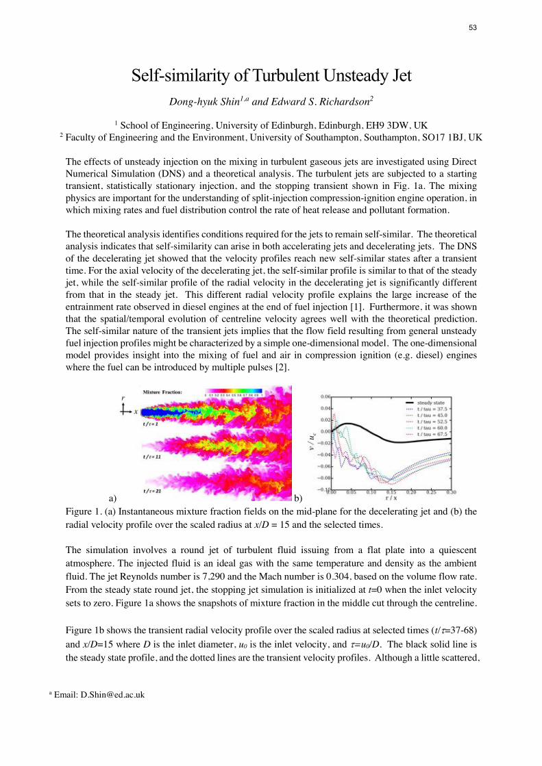
Self-similarity of Turbulent Unsteady Jet

Dong-hyuk Shin1,a and Edward S. Richardson2

1 School of Engineering, University of Edinburgh, Edinburgh, EH9 3DW, UK 2 Faculty of Engineering and the Environment, University of Southampton, Southampton, SO17 1BJ, UK

The effects of unsteady injection on the mixing in turbulent gaseous jets are investigated using Direct Numerical Simulation (DNS) and a theoretical analysis. The turbulent jets are subjected to a starting transient, statistically stationary injection, and the stopping transient shown in Fig. 1a. The mixing physics are important for the understanding of split-injection compression-ignition engine operation, in which mixing rates and fuel distribution control the rate of heat release and pollutant formation. The theoretical analysis identifies conditions required for the jets to remain self-similar. The theoretical analysis indicates that self-similarity can arise in both accelerating jets and decelerating jets. The DNS of the decelerating jet showed that the velocity profiles reach new self-similar states after a transient time. For the axial velocity of the decelerating jet, the self-similar profile is similar to that of the steady jet, while the self-similar profile of the radial velocity in the decelerating jet is significantly different from that in the steady jet. This different radial velocity profile explains the large increase of the entrainment rate observed in diesel engines at the end of fuel injection [1]. Furthermore, it was shown that the spatial/temporal evolution of centreline velocity agrees well with the theoretical prediction. The self-similar nature of the transient jets implies that the flow field resulting from general unsteady fuel injection profiles might be characterized by a simple one-dimensional model. The one-dimensional model provides insight into the mixing of fuel and air in compression ignition (e.g. diesel) engines where the fuel can be introduced by multiple pulses [2].

a) b) Figure 1. (a) Instantaneous mixture fraction fields on the mid-plane for the decelerating jet and (b) the radial velocity profile over the scaled radius at x/D = 15 and the selected times.

The simulation involves a round jet of turbulent fluid issuing from a flat plate into a quiescent atmosphere. The injected fluid is an ideal gas with the same temperature and density as the ambient fluid. The jet Reynolds number is 7,290 and the Mach number is 0.304, based on the volume flow rate. From the steady state round jet, the stopping jet simulation is initialized at t=0 when the inlet velocity sets to zero. Figure 1a shows the snapshots of mixture fraction in the middle cut through the centreline.

Figure 1b shows the transient radial velocity profile over the scaled radius at selected times (t/W=37-68) and x/D=15 where D is the inlet diameter, u0 is the inlet velocity, and W=u0/D. The black solid line is the steady state profile, and the dotted lines are the transient velocity profiles. Although a little scattered,

a Email: D.Shin@ed.ac.uk

53

it can be observed that the radial velocity profile reaches a new self-similar state after t/W=37. Note that the radial velocities have a significantly large magnitude compared to the statistically stationary jet. This predominantly negative radial velocities following the start of the deceleration indicates the increase of entrainment, and this is consistent with the other reported observations [1]. Next, by assuming self-similarity within the unsteady jet, we show that the centreline axial velocity (uc) must take the form:

� �2 1c

B

xu

t CJ

� � � (1)

where the two parameters, J and CB are determined by the shapes of the self-similar velocity profiles. Depending on the value of J, the unsteady self-similar round jet can be in an accelerating configuration or a decelerating configuration. Figure 2a and Figure 2b plot Eq. (1) with two sets of parameters. If J < 0.5 and CB>0, the accelerating jet is possible as shown in Figure 2a. Note that the jet acceleration cannot be sustained for a very long time as the velocity given by Eq. 1 would approach infinity as it continues. If J > 0.5 and CB≥0, the decelerating jet is given, and a long term solution exists for decelerating jets, as shown in Figure 2b.

a) b) c) Figure 2. The scaled centreline axial velocity over time of (a) an accelerating jet given by Eq. (1), (b) a decelerating jet given by Eq. (1), and (c) DNS data taken at multiple axial locations in a decelerating jet. Figure 2c shows the scaled axial centreline velocities over time from DNS data at selected locations. For comparison, Eq. (1) is plotted with the best fitting parameters. After a transient time of 30W, all DNS data collapse to a single line which also aligned with the line drawn by Eq. (1). This transient time scale is consistent with the time scale in Figure 1b where the radial velocity profile reaches the self-similar state after t/W=37.

REFERENCE

[1] M.P.B. Musculus, (2009) “Entrainment waves in decelerating transient turbulent jets”, Journal of Fluid

Mechanics. vol. 638, pp. 117-140.

[2] J. W. Anders, V. Magi & J. Abraham, (2008) “A Computational Investigation of the Interaction of Pulses

in Two-Pulse Jets”, Numerical Heat Transfer, vol., 54, pp. 999-1021.

54

Implicit DNS of Numerical Combustion with Detailed Chemistry

Nadeem A. Malik

Department of Mathematics & Statistics, King Fahd University of Petroleum & Minerals, Dhahran 3126, Saudi Arabia

namalik@kfupm.edu.sa and nadeem_malik@cantab.net Implicit methods are well known to be more stable than explicit methods, which is especially important for highly stiff numerical systems. The drive towards more accurate thermochemical-fluid simulations with realistic chemistry for predicting minor species and particulates provides an opportunity for developing such new methods. A recent advance has been the development of an implicit method, TARDIS (Transient Advection Reaction Diffusion Implicit Simulations) [1-4], which features the coupling of the fully compressible flow to the comprehensive chemistry and detailed multicomponent transport properties; it resolves the time and spatial scales in the stiff thermochemical system – an important step towards ’realistic’ combustion simulations. Here, we report on some of the fundamental problems addressed by using TARDIS. In the first study, transient premixed hydrogen/air flames contracting through inhomogeneous fuel distributions and subjected to stretch and pressure oscillations are investigated numerically using TARDIS. The impact of increasing positive and negative stretch is investigated through the use of planar, cylindrical and spherical geometries, in H2/air flames [1,3] and CH4/air flames [2]. The flame relaxation number 𝑛𝑅 = 𝜏𝑅/𝜏𝐿 (𝜏𝑅 is the time that the flame takes to return to the mean equilibrium conditions after initial disturbance; 𝜏𝐿 is a flame time scale) decreases by 10% in negatively stretched contracting H2/air flames, in contrast to the two positively stretched expanding H2/air and CH4/air flames where 𝑛𝑅 decreased by 40%. 𝑛𝑅 appears to much more sensitive to variations in positive/negative curvature than to the thermo-chemistry of different flame types. 𝑛𝑅 may thus be a useful indicator of the strength of flame-curvature coupling. Figure 1. In a second study [4], a question of great importance in combustion theory is addressed: how to characterise the flame length and time scales. There is no universally accepted theory as yet. One of the most important concepts in combustion theory is flame stretch, 𝑍 = (𝑑𝐴(𝑡)/𝑑𝑡)/𝐴(𝑡), which is the relative rate of change of an element of surface area 𝐴(𝑡) on the flame surface. Stretch quantifies the effect of local heat release of a propagating flame on variations in the surface area along the flame front and the associated local flame curvature; as such stretch is sensitive to the local strain and to the flame geometry, which is turn affect physical quantities like the flame speed Sn. For axi-symmetric and spherically symmetric flames stretch scales like, 𝑍(𝑟) = 1/𝑟𝑢 where 𝑟𝑢 is the flame radius. We explore the thermochemical structure of stretched laminar flames through simulations of eight premixed flames at atmospheric pressure and at stoichiometric mixture levels: expanding and contracting H2/air and CH4/air flames in axi-symmetric and spherical geometries. The aim is to explore consistent methods of characterising the flame thickness and the associated time scales. Figure 2.

55

REFERENCES [1] Malik N.A. & Lindstedt R.P. “The response of transient inhomogeneous flames to pressure fluctuations and stretch: planar and outwardly propagating hydrogen/air flames”. Combust. Sci. Tech. 182:9, 2010. [2] Malik N. A. & Lindstedt R.P. “The response of transient inhomogeneous flames to pressure fluctuations and stretch: planar and outwardly propagating methane/air flames”. Combustion Science and Technology, 184:10-11, 1799—1817, 2012. [3] Malik N. A., Korakianitis T., & Lovas T. “A numerical study of the response of transient inhomogeneous flames to pressure fluctuations and negative stretch in contracting hydrogen/air flames”. Submitted to PLOS ONE, 2016. http://arxiv.org/abs/1602.00270. [4] Malik N. A. “Non-linear power laws in stretched flame velocities in finite thickness flames: a numerical study using realistic chemistry”. Combust. Sci. Tech. 184:10-11, 1787—1798, 2012.

Figure 1. The burning velocity 𝑺𝒏 [m/s] against time 𝒕 [ms]. H2/Air system.

Figure 2. The flame structure. H2/Air (left) and CH4/Air systems.

Spherical Cylindrical Planar

Bur

ning

vel

ocity

S

m/s

Radius [mm] Radius [mm] Radius [mm]

Mo

le f

ract

ion

Fra

ctio

n

Mo

le f

ract

ion

56

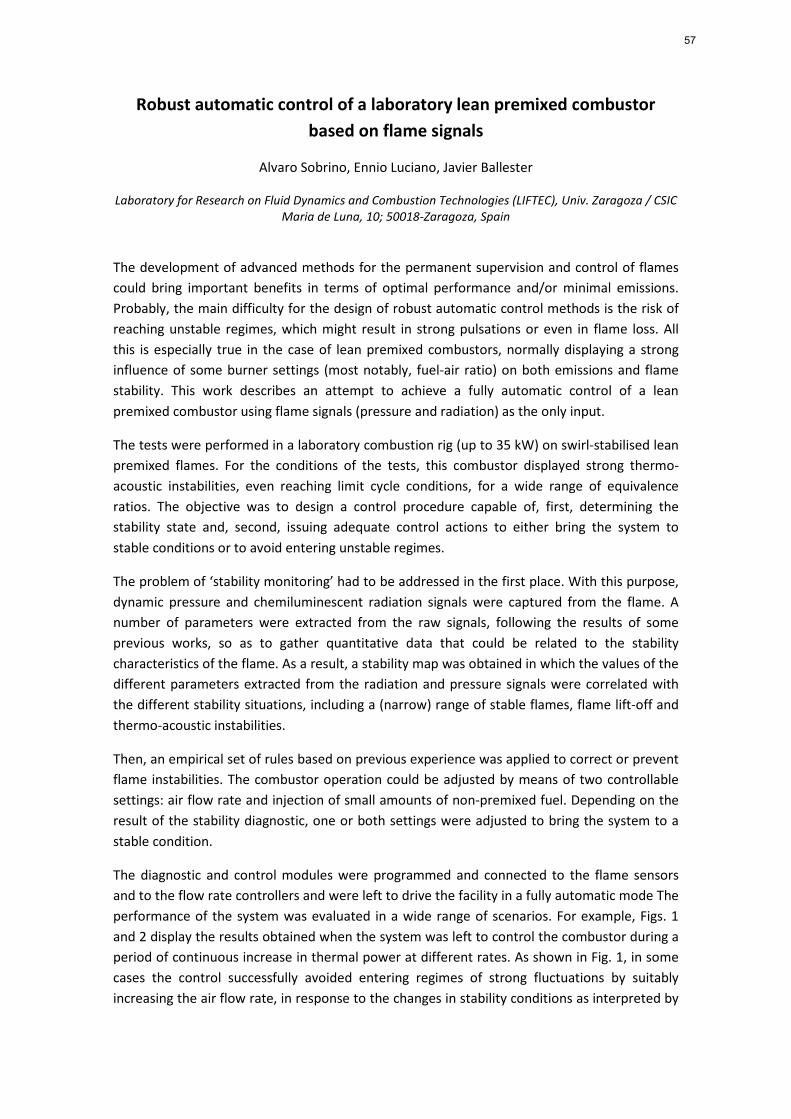
Robust automatic control of a laboratory lean premixed combustor based on flame signals

Alvaro Sobrino, Ennio Luciano, Javier Ballester

Laboratory for Research on Fluid Dynamics and Combustion Technologies (LIFTEC), Univ. Zaragoza / CSIC Maria de Luna, 10; 50018-Zaragoza, Spain

The development of advanced methods for the permanent supervision and control of flames

could bring important benefits in terms of optimal performance and/or minimal emissions.

Probably, the main difficulty for the design of robust automatic control methods is the risk of

reaching unstable regimes, which might result in strong pulsations or even in flame loss. All

this is especially true in the case of lean premixed combustors, normally displaying a strong

influence of some burner settings (most notably, fuel-air ratio) on both emissions and flame

stability. This work describes an attempt to achieve a fully automatic control of a lean

premixed combustor using flame signals (pressure and radiation) as the only input.

The tests were performed in a laboratory combustion rig (up to 35 kW) on swirl-stabilised lean

premixed flames. For the conditions of the tests, this combustor displayed strong thermo-

acoustic instabilities, even reaching limit cycle conditions, for a wide range of equivalence

ratios. The objective was to design a control procedure capable of, first, determining the

stability state and, second, issuing adequate control actions to either bring the system to

stable conditions or to avoid entering unstable regimes.

The problem of ‘stability monitoring’ had to be addressed in the first place. With this purpose,

dynamic pressure and chemiluminescent radiation signals were captured from the flame. A

number of parameters were extracted from the raw signals, following the results of some

previous works, so as to gather quantitative data that could be related to the stability

characteristics of the flame. As a result, a stability map was obtained in which the values of the

different parameters extracted from the radiation and pressure signals were correlated with

the different stability situations, including a (narrow) range of stable flames, flame lift-off and

thermo-acoustic instabilities.

Then, an empirical set of rules based on previous experience was applied to correct or prevent

flame instabilities. The combustor operation could be adjusted by means of two controllable

settings: air flow rate and injection of small amounts of non-premixed fuel. Depending on the

result of the stability diagnostic, one or both settings were adjusted to bring the system to a

stable condition.

The diagnostic and control modules were programmed and connected to the flame sensors

and to the flow rate controllers and were left to drive the facility in a fully automatic mode The

performance of the system was evaluated in a wide range of scenarios. For example, Figs. 1

and 2 display the results obtained when the system was left to control the combustor during a

period of continuous increase in thermal power at different rates. As shown in Fig. 1, in some

cases the control successfully avoided entering regimes of strong fluctuations by suitably

increasing the air flow rate, in response to the changes in stability conditions as interpreted by

57

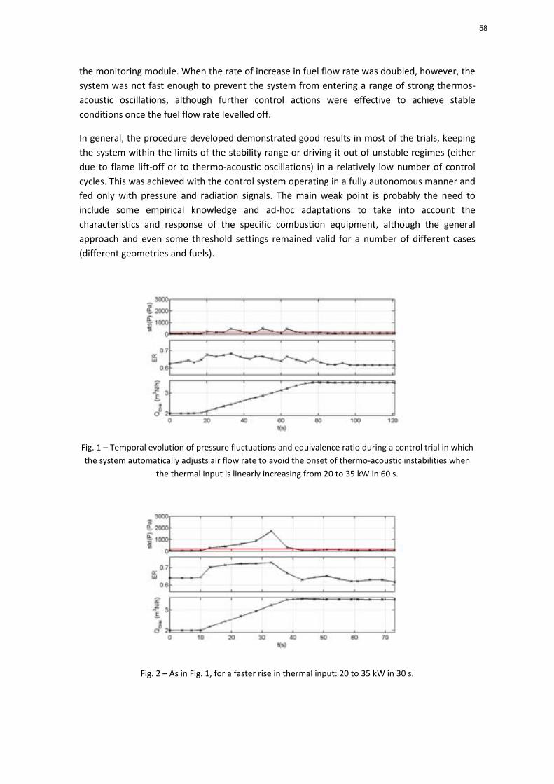
the monitoring module. When the rate of increase in fuel flow rate was doubled, however, the system was not fast enough to prevent the system from entering a range of strong thermos-acoustic oscillations, although further control actions were effective to achieve stable conditions once the fuel flow rate levelled off.

In general, the procedure developed demonstrated good results in most of the trials, keeping the system within the limits of the stability range or driving it out of unstable regimes (either due to flame lift-off or to thermo-acoustic oscillations) in a relatively low number of control cycles. This was achieved with the control system operating in a fully autonomous manner and fed only with pressure and radiation signals. The main weak point is probably the need to include some empirical knowledge and ad-hoc adaptations to take into account the characteristics and response of the specific combustion equipment, although the general approach and even some threshold settings remained valid for a number of different cases (different geometries and fuels).

Fig. 1 – Temporal evolution of pressure fluctuations and equivalence ratio during a control trial in which the system automatically adjusts air flow rate to avoid the onset of thermo-acoustic instabilities when

the thermal input is linearly increasing from 20 to 35 kW in 60 s.

Fig. 2 – As in Fig. 1, for a faster rise in thermal input: 20 to 35 kW in 30 s.

58

Spectral identity of gas fuels: temperature effect

Nelson Alvesa, Teodoro P. Trindadeb, Edgar C. Fernandesa

aInstituto Superior Técnico, Mechanical Engineering Department, University of Lisbon,

Av. Rovisco Pais, 1049-001 Lisboa, Portugal

bISEL - Instituto Superior de Engenharia de Lisboa, Chemical Engineering Department,

R. Conselheiro Emídio Navarro 1, 1959-007 Lisboa, Portugal

This study investigate the influence of flame temperature on the chemilumi-nescence response of laminar premixed gas flames. In a previous work [1]the chemiluminescence technique was used to establish a characteristic spec-tral identity of methane (CH4) and propane (C3H8) fuels, which was capableto detect the unburned gas composition on binary CH4/C3H8 blends. Thebasis of chemiluminescence fuel identification is supported on the propertyof total chemiluminescence light that, when purged of continuum-wide bandof CO⇤

2 emitters, exhibit a characteristic emission distribution between OH⇤,CH⇤ and C⇤

2 band families. To typify the distribution of flame radiation, anewly parameter termed “chemiluminescence fraction” is proposed, generallydefined as the ratio between an emitter intensity to the total chemilumines-cence. Figure 1 shows on a ternary diagram the characteristic chemilumi-nescence curves of CH4 and C3H8 obtained at room conditions in a range ofthermal power (0.75� 1.75 kW).

Considering Ii the local emission density of an excited radical i in a flame,and assuming that it may be described globally by an Arrhenius type formu-lation, such as:

Ii = ↵AT � e�E/RT [ F ]�1 [ O ]�2

the effect of parameters such as flame temperature T and concentrations offuel [ F ] and oxidizer [O ] species can be linked. The work presented wasdeveloped on laminar Bunsen burner flames at around stoichiometry, in therange of � = 0.80 to 1.30. From each flame, the spatially integrated emissionspectrum was acquired using a radiometrically calibrated spectrometer that

Email address: teodoro.trindade@deq.isel.ipl.pt (Teodoro P. Trindade)

Joint British, Spanish and Portuguese Section Meeting, 2016 March 5, 2016

59

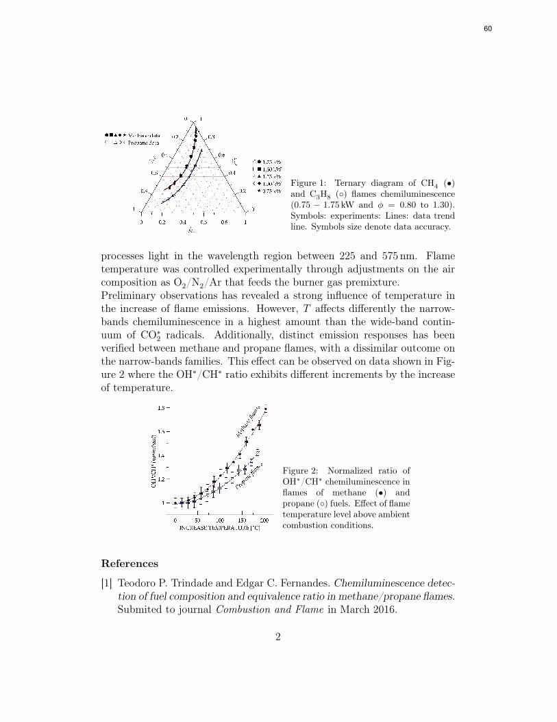
Figure 1: Ternary diagram of CH4 (•)and C3H8 (�) flames chemiluminescence(0.75 � 1.75 kW and � = 0.80 to 1.30).Symbols: experiments: Lines: data trendline. Symbols size denote data accuracy.

processes light in the wavelength region between 225 and 575 nm. Flametemperature was controlled experimentally through adjustments on the aircomposition as O2/N2/Ar that feeds the burner gas premixture.Preliminary observations has revealed a strong influence of temperature inthe increase of flame emissions. However, T affects differently the narrow-bands chemiluminescence in a highest amount than the wide-band contin-uum of CO⇤

2 radicals. Additionally, distinct emission responses has beenverified between methane and propane flames, with a dissimilar outcome onthe narrow-bands families. This effect can be observed on data shown in Fig-ure 2 where the OH⇤/CH⇤ ratio exhibits different increments by the increaseof temperature.

Figure 2: Normalized ratio ofOH⇤/CH⇤ chemiluminescence inflames of methane (•) andpropane (�) fuels. Effect of flametemperature level above ambientcombustion conditions.

References

[1] Teodoro P. Trindade and Edgar C. Fernandes. Chemiluminescence detec-

tion of fuel composition and equivalence ratio in methane/propane flames.Submited to journal Combustion and Flame in March 2016.

2

60