Tampere University of Technology

Joint Mitigation of Nonlinear RF and Baseband Distortions in Wideband Direct-Conversion Receivers

CitationGrimm, M., Allen, M., Marttila, J., Valkama, M., & Thomä, R. (2014). Joint Mitigation of Nonlinear RF andBaseband Distortions in Wideband Direct-Conversion Receivers. IEEE Transactions on Microwave Theory andTechniques, 62(1), 166-182. DOI: 10.1109/TMTT.2013.2292603Year2014

VersionPeer reviewed version (post-print)

Link to publicationTUTCRIS Portal (http://www.tut.fi/tutcris)

Published inIEEE Transactions on Microwave Theory and Techniques

DOI10.1109/TMTT.2013.2292603

Copyright© 2014 IEEE. Personal use of this material is permitted. Permission from IEEE must be obtained for all otheruses, in any current or future media, including reprinting/republishing this material for advertising or promotionalpurposes, creating new collective works, for resale or redistribution to servers or lists, or reuse of anycopyrighted component of this work in other works.

Take down policyIf you believe that this document breaches copyright, please contact tutcris@tut.fi, and we will remove access tothe work immediately and investigate your claim.

Download date:17.07.2018

IEEE TRANSACTIONS ON MICROWAVE THEORY AND TECHNIQUES, VOL. ?, NO. ?, ? 2013 1

Joint Mitigation of Nonlinear RF and Baseband

Distortions in Wideband Direct-Conversion

ReceiversMichael Grimm, Markus Allén, Student Member, IEEE, Jaakko Marttila, Student Member, IEEE,

Mikko Valkama, Member, IEEE, and Reiner Thomä, Fellow, IEEE

Abstract—Software-defined radio technology is experiencingmore and more attention in modern communication and radarsystems. The main practical challenge in deploying such tech-nology is related to achieving sufficient linearity and spurious-free dynamic range in the RF front-end, especially in low-costmass-product devices. This paper focuses on the analysis anddigital mitigation of nonlinear distortion in software-definedradio devices, building on wideband multicarrier/multiradiodirect-conversion receiver principle where a wide collection ofradio frequencies is I/Q down-converted as a whole. A completebehavioral model for the total nonlinear distortion of the wholereceiver chain is first derived, taking into account the third-ordernonlinear distortion effects in all individual components, namelyRF low-noise amplifier, I/Q mixer and baseband I/Q amplifiers.Stemming from this modeling, adaptive digital feed-forward lin-earization structure is then developed, to efficiently mitigate thejoint nonlinear distortion of the whole receiver. The effectivenessof this approach is verified through extensive simulations andactual RF system measurements with a commercially availablesoftware defined radio platform, which clearly outperforms theexisting state-of-the-art methods that do not jointly consider RFand baseband nonlinearities.

Index Terms—Cognitive radio, software-defined radio, adap-tive signal processing, linearization techniques, nonlinear distor-tion, interference cancellation, intermodulation distortion

I. INTRODUCTION

THE commercial availability of various software-defined

radio (SDR) platforms has provided an easy way for

experimental radio system research with a highly flexible RF

interface. This plays an important role in communications and

passive radar applications. Multiradio basestation transceivers

in mobile cellular radio systems, with capability of simultane-

ous transmission and reception at multiple cellular bands and

Manuscript received July 8, 2013; revised November 8, 2013; acceptedNovember 15, 2013. This work was supported by the Finnish FundingAgency for Technology and Innovation (Tekes) under the project "EnablingMethods for Dynamic Spectrum Access and Cognitive Radio," the Academyof Finland under the project 251138 "Digitally-Enhanced RF for CognitiveRadio Devices," Austrian Competence Center in Mechatronics (ACCM), TUTGraduate School, Nokia Foundation, and the International Graduate Schoolon Mobile Communications supported by the German Research Foundation(DFG GRK1487).

M. Grimm and R. Thomä are with the Electronic Measurement ResearchLab, Institute for Information Technology, Ilmenau University of Tech-nology, 98684 Ilmenau, Germany (e-mail: michael.grimm@tu-ilmenau.de,reiner.thomae@tu-ilmenau.de).

M. Allén, J. Marttila, and Mikko Valkama are with the Department of Elec-tronics and Communications Engineering, Tampere University of Technol-ogy, P.O. Box 692, FI-33101 Tampere, Finland (e-mail: markus.allen@tut.fi,jaakko.marttila@tut.fi, mikko.e.valkama@tut.fi).

access technologies, form a good example of potential SDR

deployment scenarios. In this kind of flexible RF spectrum use,

obtaining sufficient linearity and spurious-free dynamic range

(SFDR) is one of the biggest challenges [1], especially if one

wideband RF chain is deployed, instead of multiple parallel

RF chains. Similar challenges are faced in wideband cognitive

radio (CR) sensing receivers, as discussed, e.g., in [2] when

trying to extract wideband instantaneous radio environment

knowledge.

This paper focuses on nonlinear distortion and SFDR chal-

lenges in wideband multicarrier/multiradio direct-conversion

receivers (DCRs) where a wide collection of radio frequencies

is in-phase/quadrature (I/Q) down-converted as a whole. In

contrast to the transmitter side, the perspective on nonlinear

distortion at receiver side is fundamentally different. In trans-

mitters, especially when simultaneously transmitting multiple

carriers of a single or possibly even multiple radio access

technologies through a single power amplifier (PA), there

are big challenges with obtaining sufficient linearity [3]. In

wideband multiradio receivers, however, nonlinear distortion

problems are even more challenging due to the presence of

multiple unknown signals, with different power levels and

dynamics due to the specific propagation conditions. As the

dynamic range within the overall down-converted frequency

range can be in the order of 60–100 dB [1], [2], such wideband

receivers are extremely prone to any imperfections in the

RF analog components. In general, essential receiver RF

impairments include DC offsets due to self-mixing, oscillator

phase noise, I/Q imbalance, and nonlinear distortions [1]. In

particular, I/Q imbalance and nonlinear distortion effects of the

receiver components can severely degrade the demodulation

performance at weak signal bands, and also heavily affect the

reliability of spectrum monitoring or sensing in CR [2], [4]–

[8]. In multiradio receivers, the most challenging scenarios

arise when the same wideband RF chain is simultaneously

receiving multiple GSM, UMTS/WCDMA and LTE carriers,

and some of them are close to the maximum allowed blocking

signal level whereas some others are close to the receiver

sensitivity level. In these kind of scenarios, the intermodulation

distortion (IMD) of strong blocking carriers can easily mask

the weaker signals, thus requiring extreme linearity from the

receiver. Similar challenges exist in wideband CR sensing

receivers, where some of the primary user signals can be close

to the thermal noise floor, but should still be identified in

the presence of other strong co-existing signals. Additionally,

2 IEEE TRANSACTIONS ON MICROWAVE THEORY AND TECHNIQUES, VOL. ?, NO. ?, ? 2013

strong nonlinear distortion can cause false alarms in spectrum

sensing when a vacant channel contains the distortion and is

falsely interpreted as being occupied by a primary user [7].

Compared to conventional receiver architectures with multiple

intermediate frequency (IF) stages, most of the selectivity in

DCR front-ends is implemented at the baseband (BB) or only

in digital domain in favor of flexibility and operation over

a wide bandwidth. Therefore, linearity and dynamic range

requirements are extremely stringent.

In this paper, we address the modeling and digital mitigation

of nonlinear distortion of all the essential RF analog compo-

nents of a wideband DCR. In the existing literature, mitigating

receiver nonlinear distortion by means of BB digital signal

processing has been proposed in [9], [10], and subsequently

followed in [7], [11]–[15], among others. Furthermore, specific

even-order distortion mitigation in classical narrowband DCR

context is addressed in [16]. In all these works, specific refer-

ence models of considered nonlinear components are applied,

either in analog or digital domain, to regenerate considered

distortion products and to subtract them from the received

signal. Previous works [7], [9], [10], [12], [13], [17] all focus

on specific receiver component only, namely RF low-noise

amplifier (LNA), BB amplifiers or analog-to-digital converter

(ADC), whereas [14] provides specific application of distortion

mitigation to interference scenarios in GSM downlink. Fur-

thermore, customized analog receiver designs were proposed

in [11] and [12] to overcome specific limitations of entirely

digital processing based approaches.

According to the best knowledge of the authors, however,

modeling and mitigation of the nonlinearities induced by a

complete DCR chain, including RF LNA, I/Q mixer and BB

I/Q amplifiers, as well as their interaction with mixer I/Q im-

balance is missing from the existing state-of-the-art literature.

As all these components behave in a nonlinear manner in prac-

tice, understanding and being able to mitigate the joint nonlin-

ear distortion effects are seen critical and therefore addressed

in this paper. Contrary to conventional spectral regrowth

around the distortion-producing signal, distortion products in

DCRs are created by RF and BB receiver components and

may fall within the BB bandwidth. Thus, we first derive the

complete behavioral model for the total nonlinear distortion,

which takes into account the third-order nonlinear distortion of

the RF LNA, I/Q imbalance of the I/Q mixer, and third-order

nonlinear distortion of the mixer and BB amplifiers. Individual

component modeling is kept at third-order level since third-

order distortion is the most dominant one in practice, and the

presentation and notations are also simplified. Notice, however,

that from the total receiver distortion modeling perspective,

up to ninth-order distortion modeling is supported by joint

modeling of RF and BB distortion. Stemming from this mod-

eling, efficient DSP-based linearization structure, together with

practical adaptive filtering based learning algorithms, are then

developed. All the signal processing developments are non-

data-aided (blind), as in general received signals are unknown

due to unknown modulating data and unknown propagation

conditions. Thus, the developed linearization can be carried

out in the very first stages of the receiver digital front-end,

prior to any modulation- or system-specific processing and

carrier-/timing synchronization. This is a substantial practi-

cal benefit, compared to data-aided approaches, since heavy

nonlinear distortion can also easily hinder the operation of,

e.g., synchronization algorithms. Finally, extensive computer

simulation results, as well as actual RF system measurements

with commercial SDR platform, namely Universal Software

Radio Peripheral (USRP) [18], are provided. Based on the

obtained results, the developed linearization scheme clearly

outperforms the existing reference methods, which can only

suppress the effects of individual receiver components. Thus,

the developed linearization solution can be seen as one key

enabling technique towards practical deployment of SDR

technology with digitally-enhanced wideband RF front-ends.

The outline of the remainder of the paper is as follows.

In the following Section II, nonlinear distortion effects and

mirror-frequency interference created in the DCR chain are

discussed and modeled in detail, first component-wise and

then accumulated into a total composite model. Based on

that joint model, Section III then develops the proposed

digital mitigation architecture and associated parameter learn-

ing algorithms. Simulation and RF measurement results are

presented and analyzed in Section IV, whereas Section V

gives further discussions, result analysis, and outlook on future

work. Finally, conclusions are drawn in Section VI.

II. NONLINEAR DISTORTION ANALYSIS IN WIDEBAND

DIRECT-CONVERSION RECEIVERS

This section gives a detailed description of nonlinearities

occurring in DCRs and a derivation of a complete mathemat-

ical model, combining RF and BB stage nonlinearities.

A. Receiver Architecture and Signal Scenario of Interest

DCRs have become more popular due to their inherent

advantages over superheterodyne receivers [1], [19]. The DCR

architecture is compact since the frequency translation from

RF to BB is performed by a single mixing stage. The direct

down-conversion allows signal amplification and filtering at

BB, therefore, decreasing power consumption and simplifying

image rejection. Altogether, these benefits ease the implemen-

tation of the whole receiver as a monolithic integrated circuit

and decrease its manufacturing cost. However, DCRs suffer

from the RF and BB impairments, such as I/Q imbalance and

nonlinear distortion, as discussed in Section I.

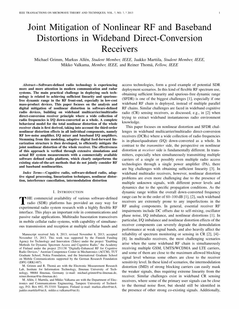
Fig. 1 depicts a basic block diagram of a DCR with quadra-

ture down-conversion, which generally consists of analog

RF, mixer, analog BB, and digital post-processing stages. In

practice, analog RF and BB stages suffer from unavoidable

nonlinear behavior. Distortions that are created at the RF

amplifier are typically dominating distortions created at the BB

stages. However, they depend on the deployed components.

In addition, the RF filtering provides very low selectivity.

Thus, strong out-of-band signals can easily enter the front-end

amplification and mixing stages. Beside receiver nonlinearity,

I/Q imbalance of the mixer and the BB I/Q branches cause

distorting mirror signal components that may interfere with

other useful signals.

GRIMM et al.: JOINT MITIGATION OF NONLINEAR RF AND BASEBAND DISTORTIONS IN WIDEBAND DIRECT-CONVERSION RECEIVERS 3

0◦

90◦

ADC

ADCLNA

Bandpass

Baseband Processing

Digital

LO

Lowpass

Lowpass

RF Front-End

Filter

Filter

FilterPost-

Processing

Fig. 1. Conceptual direct-conversion receiver block diagram. In widebandreceiver scenario, multiple carriers and possibly also radio access technologiesare received simultaneously, and selectivity filtering is implemented in thedigital parts.

The most challenging case in deploying the direct-

conversion radio architecture is the wideband multicar-

rier/multiradio scenario where the down-converted signal con-

tains multiple carriers of multiple co-existing radio access

technologies, throughout the whole receiver chain through the

A/D interface. This kind of scenario leads to high dynamic

range signal configurations with weak and strong signals si-

multaneously present. It is then likely that nonlinear distortions

caused by strong signals fall on top of weak desired signals

or leak into free frequency bands in case of CR sensing

receiver. In CR context, free frequency bands are typically

called white spaces [4]. Receiver distortion may mask a white

space so that spectrum sensing algorithms falsely consider

it to be occupied, which causes the CR to be less efficient

from the spectrum exploitation point of view. Since multiple

signals from different sources may, in general, arrive at the

antenna input, mitigation of distortions created in the receiver

becomes more challenging than in a transmitter, where the

signal sources are well-known inside the device. Therefore,

proper modeling of DCRs is essential to clean the whole BB

from all distortions stemming from the strong input signals.

B. RF Nonlinearities

In this paper, BB equivalent signal modeling is used as it is

notationally convenient and widely adopted convention [20].

The received bandpass signal xRF(t) can be presented as

xRF(t) = 2Re[x(t)ejωct] = x(t)ejωct + x∗(t)e−jωct, (1)

where ωc is the angular center frequency of the total RF

signal to be down-converted and x(t) is the corresponding BB

equivalent signal of xRF(t) ((·)∗ denotes complex conjugate).

Notice that in this notation, in case of wideband multicarrier

down-conversion, the BB equivalent signal x(t) contains all

individual carrier waveforms at different complex IFs. Fur-

thermore, x(t) is defined as

x(t) = A(t)ejφ(t) = xI(t) + jxQ(t), (2)

where A(t) and φ(t) are the total envelope and phase of the

overall down-converted RF signal x(t), whereas xI(t) and

xQ(t) denote the corresponding composite I and Q signals,

respectively. The signal model (2) provides a starting point

for modeling RF and BB nonlinearities of DCRs. This leads

to the structure shown in Fig. 2, where also simplified BB

equivalent spectra are illustrated, with only one active carrier

for visualization purposes. Next, more detailed modeling of

the RF LNA nonlinearities is addressed.

From the actual RF signal perspective, the RF nonlinearities

can be modeled using a generalized Hammerstein model

yRF(t) = b1(t) ∗ xRF(t) + b2(t) ∗ x2RF(t) + . . . , (3)

where b1(t), b2(t), b3(t), . . . are impulse responses for each

nonlinearity order taking memory effects into account [21]. In

practice, (3) models the nonlinear behavior of the LNA in the

RF stage. Using this notation, the input of the LNA in Fig. 1 is

xRF(t) and the output is yRF(t). While (3) provides the general

model, it is possible to simplify it and still capture the most

essential behavior of the DCR. Even-order RF nonlinearities

produce new frequency components, which are in most cases

far away from ωc and thus most likely to be filtered out. For

example, an equation obtained from (1) and (3) for the second-

order nonlinearity

x2RF(t) = 2x(t)x∗(t) + x2(t)ej2ωct + [x∗(t)]2e−j2ωct (4)

illustrates the new frequencies appearing around ±2ωc and

DC (zero frequency), but no IMD components are created

within the interesting RF bandwidth around ωc. However, IMD

contained in xRF(t) cannot be seen directly from (4). These

even-order RF IMD components are usually not harmful,

except if the RF front-end is extremely wideband and xRF(t)consists of several strong signals, which are far away from

each other [2]. Even in this case, the even-order effects

are not significant when proper circuit design methodologies

providing high second-order intercept points are employed [2],

[22]. In addition, the even-order nonlinearities induce spectral

content around DC, such as 2x(t)x∗(t) = 2A2(t) in (4), but it

can be removed effectively with AC-coupling or filtering [2],

[23]. Odd-order nonlinearities are, however, more critical since

they cause new frequency components near ωc, i.e., within the

total frequency band of interest. In practice, the third-order

nonlinearity is usually the strongest and the only one among

the RF nonlinearity orders that appears clearly above the noise

level. Therefore, a simplified RF nonlinearity model

y′RF(t) = a1xRF(t) + a2x3RF(t) (5)

is considered here, in which memory effects are omitted for

notational simplicity and hence scalar coefficients a1 and a2,

instead of filters b1(t) and b3(t), are used. This leads to

the widely-used memoryless polynomial model [10], [24].

The lack of memory simplifies the notation in this analysis

so that the most essential interpretations of the nonlinearity

phenomenon can be made more easily. The memory effects

are then taken into account later in the next section when

impairment mitigation is discussed. The coefficients a1 and a2are chosen to be complex in order to model AM/PM distortion

of the LNA [24].

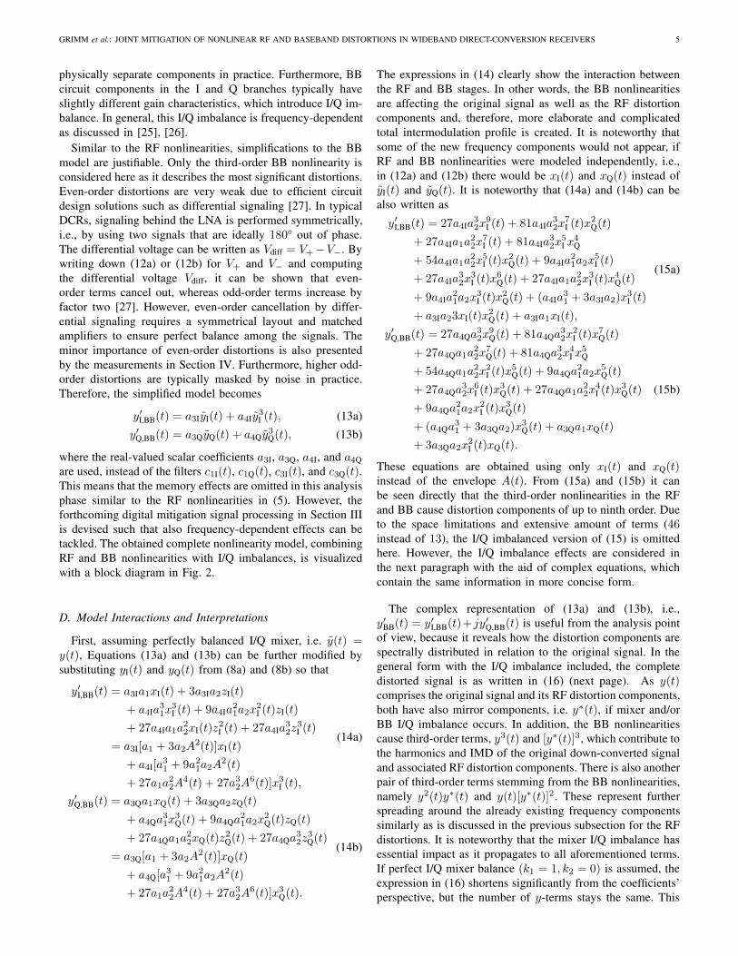
To further analyze the new spectral content by the third-

order RF nonlinearity, the latter term of (5) can be written as

a2x3RF(t) = a2{x(t)e

jωct + x∗(t)e−jωct}3

= a2{x3(t)ej3ωct + [x∗(t)]3e−j3ωct

+ 3x2(t)x∗(t)ejωct + 3x(t)[x∗(t)]2e−jωct}.

(6)

4 IEEE TRANSACTIONS ON MICROWAVE THEORY AND TECHNIQUES, VOL. ?, NO. ?, ? 2013

(·)2(·)∗

(·)3

(·)3(·)∗

a1

3a2

a3I

a4I

a3Q

a4Q

k1

k2

Mixer and BB Nonlinearity Model

RF Nonlinearity Model Mixer I/Q Imbalance ModelIm

Re

j

ffff

x(t) y(t) yI(t)

yQ(t)

y(t) y′BB(t)

fIFfIFfIFfIF −fIF−fIF 3fIF−3fIF

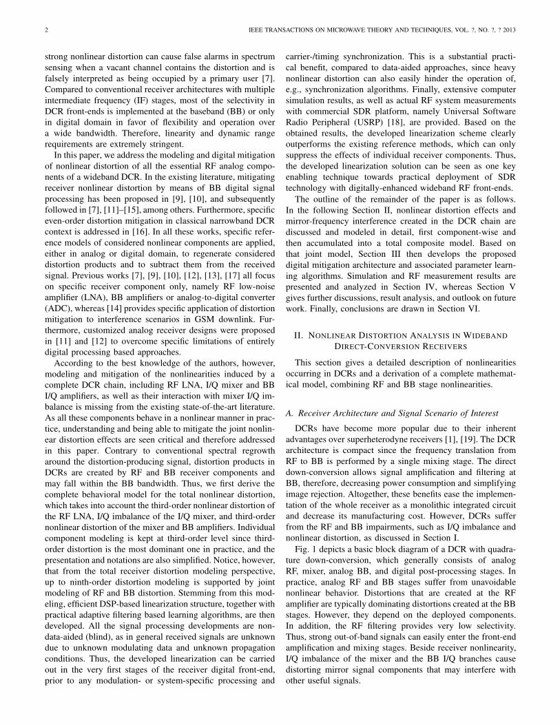
Fig. 2. Cascaded model considering third-order RF and BB nonlinearities in the presence of mixer and BB I/Q imbalance. Due to the generality of thenonlinearity models, they also take mixer nonlinearities into account. The spectrum illustrations are sketched for BB equivalent signals matching to themathematical modeling in the paper, and only a single carrier is shown for visualization purposes.

From (6) it is apparent that there is only one term that causes

new frequency content around ωc, i.e., 3a2x2(t)x∗(t)ejωct.

The effective RF nonlinearity contribution comes from this

particular term since it is shifted to the BB in the I/Q down-

conversion stage whereas the other three terms in (6) do not

hit the BB and are hence filtered out. Therefore, the essential

BB equivalent form of (5) after the BB filtering becomes

y(t) = yI(t) + jyQ(t)

= a1x(t) + 3a2x2(t)x∗(t)

= a1x(t) + 3a2A2(t)x(t)

= a1x(t) + 3a2z(t).

(7)

The second-last form of (7) is stemming from the fact that

x(t)x∗(t) = |x(t)|2= A2(t). An auxiliary variable z(t) is

introduced here to denote the RF distortion contribution and

make some of the further equations easier to interpret. The

real and imaginary parts of y(t) can be written as

yI(t) = a1xI(t) + 3a2[x3I (t) + xI(t)x

2Q(t)]

= a1xI(t) + 3a2A2(t)xI(t)

= a1xI(t) + 3a2zI(t),

(8a)

yQ(t) = a1xQ(t) + 3a2[x2I (t)xQ(t) + x3

Q(t)]

= a1xQ(t) + 3a2A2(t)xQ(t)

= a1xQ(t) + 3a2zQ(t).

(8b)

It is worth noticing that the term 3a2A2(t)x(t) only causes

distortion around the center frequency of x(t). However, the

bandwidth of the distortion is wider than of x(t), because of

the multiplication with the squared envelope A2(t).After the LNA, the signal goes through a wideband I/Q

down-conversion stage as depicted in Fig. 1. In practice, an

I/Q mixer cannot provide exactly 90° phase shift as desired but

sustains a phase mismatch of φm (rad). Additionally, the I/Q

mixer suffers from a relative amplitude mismatch gm between

the I and Q branches. These mismatches cause I/Q imbalance,

which is seen as mirroring of frequency content of y(t). More

detailed information about I/Q imbalance can be found in [25],

[26], and references therein. The I/Q imbalance of the down-

conversion stage is here modeled as

y(t) = k1y(t) + k2y∗(t), (9)

where the complex mismatch coefficients are

k1 =(

1 + gme−jφm

)

/2, (10a)

k2 =(

1− gmejφm

)

/2. (10b)

With perfect I/Q balance, gm = 1, φm = 0 and hence k1 = 1,

k2 = 0. The RF-distorted signal with I/Q imbalance y(t) =yI(t) + jyQ(t) can now be expressed as

yI(t) = yI(t), (11a)

yQ(t) = gm cos(φm)yQ(t)− gm sin(φm)yI(t). (11b)

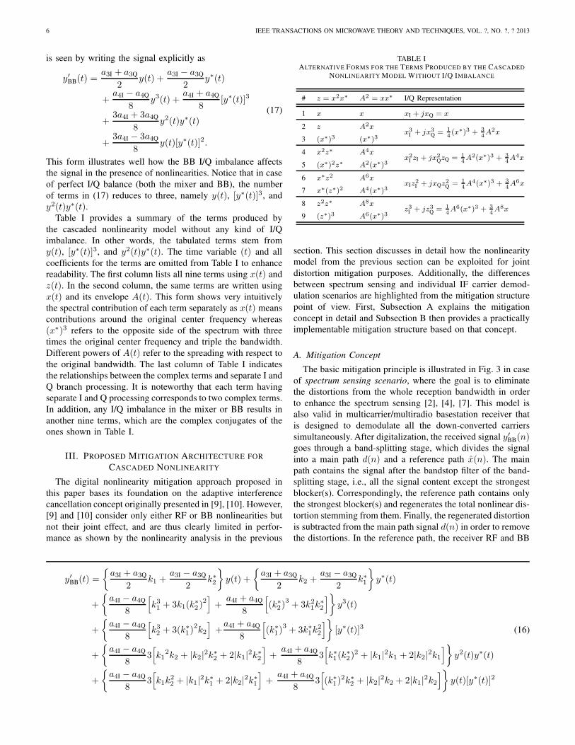
The results presented in (8) and (11) are important in a sense

that y(t) is the signal distorted by both RF nonlinearities

and mixer I/Q imbalance, and hence describes their joint

impact. More specifically, the signal at this point contains

the intermodulation distortion created by the RF LNA and its

mirror image symmetrically around zero-frequency, as well as

the actual mirror image of the ideal signal. These are illustrated

in Fig. 2. Next, the I and Q signals become further distorted

through mixer and baseband nonlinearities. This is elaborated

further in the following subsection.

C. Mixer and Baseband Nonlinearities

BB nonlinearity modeling differs from RF nonlinearities in

such a way that in the BB there are physically separate I and

Q branches in which the nonlinearities occur independently.

In general, for the distorted BB signal yBB(t) = yI,BB(t) +jyQ,BB(t), the generalized Hammerstein model is

yI,BB(t) = c1I(t) ∗ yI(t) + c2I(t) ∗ y2I (t) + . . . , (12a)

yQ,BB(t) = c1Q(t) ∗ yQ(t) + c2Q(t) ∗ y2Q(t) + . . . , (12b)

where c1I(t), c2I(t), c3I(t), . . . and c1Q(t), c2Q(t), c3Q(t), . . .are impulse responses for each nonlinearity order in the I

and Q branches. This model basically takes into account

all the nonlinearities of BB components shown in Fig. 1,

specifically amplifiers and ADCs, and also mixers since the

I/Q mixer outputs are already at down-converted frequencies.

In the following, the term “BB nonlinearities” is used to

cover these as a whole. There are different impulse responses

for I and Q polynomials, because nonlinearities themselves

can be different in the I and Q branches since those contain

GRIMM et al.: JOINT MITIGATION OF NONLINEAR RF AND BASEBAND DISTORTIONS IN WIDEBAND DIRECT-CONVERSION RECEIVERS 5

physically separate components in practice. Furthermore, BB

circuit components in the I and Q branches typically have

slightly different gain characteristics, which introduce I/Q im-

balance. In general, this I/Q imbalance is frequency-dependent

as discussed in [25], [26].

Similar to the RF nonlinearities, simplifications to the BB

model are justifiable. Only the third-order BB nonlinearity is

considered here as it describes the most significant distortions.

Even-order distortions are very weak due to efficient circuit

design solutions such as differential signaling [27]. In typical

DCRs, signaling behind the LNA is performed symmetrically,

i.e., by using two signals that are ideally 180° out of phase.

The differential voltage can be written as Vdiff = V+−V−. By

writing down (12a) or (12b) for V+ and V− and computing

the differential voltage Vdiff, it can be shown that even-

order terms cancel out, whereas odd-order terms increase by

factor two [27]. However, even-order cancellation by differ-

ential signaling requires a symmetrical layout and matched

amplifiers to ensure perfect balance among the signals. The

minor importance of even-order distortions is also presented

by the measurements in Section IV. Furthermore, higher odd-

order distortions are typically masked by noise in practice.

Therefore, the simplified model becomes

y′I,BB(t) = a3IyI(t) + a4Iy3I (t), (13a)

y′Q,BB(t) = a3QyQ(t) + a4Qy3Q(t), (13b)

where the real-valued scalar coefficients a3I, a3Q, a4I, and a4Q

are used, instead of the filters c1I(t), c1Q(t), c3I(t), and c3Q(t).This means that the memory effects are omitted in this analysis

phase similar to the RF nonlinearities in (5). However, the

forthcoming digital mitigation signal processing in Section III

is devised such that also frequency-dependent effects can be

tackled. The obtained complete nonlinearity model, combining

RF and BB nonlinearities with I/Q imbalances, is visualized

with a block diagram in Fig. 2.

D. Model Interactions and Interpretations

First, assuming perfectly balanced I/Q mixer, i.e. y(t) =y(t), Equations (13a) and (13b) can be further modified by

substituting yI(t) and yQ(t) from (8a) and (8b) so that

y′I,BB(t) = a3Ia1xI(t) + 3a3Ia2zI(t)

+ a4Ia31x

3I (t) + 9a4Ia

21a2x

2I (t)zI(t)

+ 27a4Ia1a22xI(t)z

2I (t) + 27a4Ia

32z

3I (t)

= a3I[a1 + 3a2A2(t)]xI(t)

+ a4I[a31 + 9a21a2A

2(t)

+ 27a1a22A

4(t) + 27a32A6(t)]x3

I (t),

(14a)

y′Q,BB(t) = a3Qa1xQ(t) + 3a3Qa2zQ(t)

+ a4Qa31x

3Q(t) + 9a4Qa

21a2x

2Q(t)zQ(t)

+ 27a4Qa1a22xQ(t)z

2Q(t) + 27a4Qa

32z

3Q(t)

= a3Q[a1 + 3a2A2(t)]xQ(t)

+ a4Q[a31 + 9a21a2A

2(t)

+ 27a1a22A

4(t) + 27a32A6(t)]x3

Q(t).

(14b)

The expressions in (14) clearly show the interaction between

the RF and BB stages. In other words, the BB nonlinearities

are affecting the original signal as well as the RF distortion

components and, therefore, more elaborate and complicated

total intermodulation profile is created. It is noteworthy that

some of the new frequency components would not appear, if

RF and BB nonlinearities were modeled independently, i.e.,

in (12a) and (12b) there would be xI(t) and xQ(t) instead of

yI(t) and yQ(t). It is noteworthy that (14a) and (14b) can be

also written as

y′I,BB(t) = 27a4Ia32x

9I (t) + 81a4Ia

32x

7I (t)x

2Q(t)

+ 27a4Ia1a22x

7I (t) + 81a4Ia

32x

5I x

4Q

+ 54a4Ia1a22x

5I (t)x

2Q(t) + 9a4Ia

21a2x

5I (t)

+ 27a4Ia32x

3I (t)x

6Q(t) + 27a4Ia1a

22x

3I (t)x

4Q(t)

+ 9a4Ia21a2x

3I (t)x

2Q(t) + (a4Ia

31 + 3a3Ia2)x

3I (t)

+ a3Ia23xI(t)x2Q(t) + a3Ia1xI(t),

(15a)

y′Q,BB(t) = 27a4Qa32x

9Q(t) + 81a4Qa

32x

2I (t)x

7Q(t)

+ 27a4Qa1a22x

7Q(t) + 81a4Qa

32x

4I x

5Q

+ 54a4Qa1a22x

2I (t)x

5Q(t) + 9a4Qa

21a2x

5Q(t)

+ 27a4Qa32x

6I (t)x

3Q(t) + 27a4Qa1a

22x

4I (t)x

3Q(t)

+ 9a4Qa21a2x

2I (t)x

3Q(t)

+ (a4Qa31 + 3a3Qa2)x

3Q(t) + a3Qa1xQ(t)

+ 3a3Qa2x2I (t)xQ(t).

(15b)

These equations are obtained using only xI(t) and xQ(t)instead of the envelope A(t). From (15a) and (15b) it can

be seen directly that the third-order nonlinearities in the RF

and BB cause distortion components of up to ninth order. Due

to the space limitations and extensive amount of terms (46instead of 13), the I/Q imbalanced version of (15) is omitted

here. However, the I/Q imbalance effects are considered in

the next paragraph with the aid of complex equations, which

contain the same information in more concise form.

The complex representation of (13a) and (13b), i.e.,

y′BB(t) = y′I,BB(t)+ jy′Q,BB(t) is useful from the analysis point

of view, because it reveals how the distortion components are

spectrally distributed in relation to the original signal. In the

general form with the I/Q imbalance included, the complete

distorted signal is as written in (16) (next page). As y(t)comprises the original signal and its RF distortion components,

both have also mirror components, i.e. y∗(t), if mixer and/or

BB I/Q imbalance occurs. In addition, the BB nonlinearities

cause third-order terms, y3(t) and [y∗(t)]3, which contribute to

the harmonics and IMD of the original down-converted signal

and associated RF distortion components. There is also another

pair of third-order terms stemming from the BB nonlinearities,

namely y2(t)y∗(t) and y(t)[y∗(t)]2. These represent further

spreading around the already existing frequency components

similarly as is discussed in the previous subsection for the RF

distortions. It is noteworthy that the mixer I/Q imbalance has

essential impact as it propagates to all aforementioned terms.

If perfect I/Q mixer balance (k1 = 1, k2 = 0) is assumed, the

expression in (16) shortens significantly from the coefficients’

perspective, but the number of y-terms stays the same. This

6 IEEE TRANSACTIONS ON MICROWAVE THEORY AND TECHNIQUES, VOL. ?, NO. ?, ? 2013

is seen by writing the signal explicitly as

y′BB(t) =a3I + a3Q

2y(t) +

a3I − a3Q

2y∗(t)

+a4I − a4Q

8y3(t) +

a4I + a4Q

8[y∗(t)]3

+3a4I + 3a4Q

8y2(t)y∗(t)

+3a4I − 3a4Q

8y(t)[y∗(t)]2.

(17)

This form illustrates well how the BB I/Q imbalance affects

the signal in the presence of nonlinearities. Notice that in case

of perfect I/Q balance (both the mixer and BB), the number

of terms in (17) reduces to three, namely y(t), [y∗(t)]3, and

y2(t)y∗(t).Table I provides a summary of the terms produced by

the cascaded nonlinearity model without any kind of I/Q

imbalance. In other words, the tabulated terms stem from

y(t), [y∗(t)]3, and y2(t)y∗(t). The time variable (t) and all

coefficients for the terms are omitted from Table I to enhance

readability. The first column lists all nine terms using x(t) and

z(t). In the second column, the same terms are written using

x(t) and its envelope A(t). This form shows very intuitively

the spectral contribution of each term separately as x(t) means

contributions around the original center frequency whereas

(x∗)3 refers to the opposite side of the spectrum with three

times the original center frequency and triple the bandwidth.

Different powers of A(t) refer to the spreading with respect to

the original bandwidth. The last column of Table I indicates

the relationships between the complex terms and separate I and

Q branch processing. It is noteworthy that each term having

separate I and Q processing corresponds to two complex terms.

In addition, any I/Q imbalance in the mixer or BB results in

another nine terms, which are the complex conjugates of the

ones shown in Table I.

III. PROPOSED MITIGATION ARCHITECTURE FOR

CASCADED NONLINEARITY

The digital nonlinearity mitigation approach proposed in

this paper bases its foundation on the adaptive interference

cancellation concept originally presented in [9], [10]. However,

[9] and [10] consider only either RF or BB nonlinearities but

not their joint effect, and are thus clearly limited in perfor-

mance as shown by the nonlinearity analysis in the previous

TABLE IALTERNATIVE FORMS FOR THE TERMS PRODUCED BY THE CASCADED

NONLINEARITY MODEL WITHOUT I/Q IMBALANCE

# z = x2x∗ A2 = xx∗ I/Q Representation

1 x x xI + jxQ = x

2 z A2xx3

I + jx3

Q = 1

4(x∗)3 + 3

4A2x

3 (x∗)3 (x∗)3

4 x2z∗ A4xx2

I zI + jx2

QzQ = 1

4A2(x∗)3 + 3

4A4x

5 (x∗)2z∗ A2(x∗)3

6 x∗z2 A6xxIz

2

I + jxQz2

Q = 1

4A4(x∗)3 + 3

4A6x

7 x∗(z∗)2 A4(x∗)3

8 z2z∗ A8xz3I + jz3Q = 1

4A6(x∗)3 + 3

4A8x

9 (z∗)3 A6(x∗)3

section. This section discusses in detail how the nonlinearity

model from the previous section can be exploited for joint

distortion mitigation purposes. Additionally, the differences

between spectrum sensing and individual IF carrier demod-

ulation scenarios are highlighted from the mitigation structure

point of view. First, Subsection A explains the mitigation

concept in detail and Subsection B then provides a practically

implementable mitigation structure based on that concept.

A. Mitigation Concept

The basic mitigation principle is illustrated in Fig. 3 in case

of spectrum sensing scenario, where the goal is to eliminate

the distortions from the whole reception bandwidth in order

to enhance the spectrum sensing [2], [4], [7]. This model is

also valid in multicarrier/multiradio basestation receiver that

is designed to demodulate all the down-converted carriers

simultaneously. After digitalization, the received signal y′BB(n)goes through a band-splitting stage, which divides the signal

into a main path d(n) and a reference path x(n). The main

path contains the signal after the bandstop filter of the band-

splitting stage, i.e., all the signal content except the strongest

blocker(s). Correspondingly, the reference path contains only

the strongest blocker(s) and regenerates the total nonlinear dis-

tortion stemming from them. Finally, the regenerated distortion

is subtracted from the main path signal d(n) in order to remove

the distortions. In the reference path, the receiver RF and BB

y′BB(t) =

{

a3I + a3Q

2k1 +

a3I − a3Q

2k∗2

}

y(t) +

{

a3I + a3Q

2k2 +

a3I − a3Q

2k∗1

}

y∗(t)

+

{

a4I − a4Q

8

[

k31 + 3k1(k∗

2)2]

+a4I + a4Q

8

[

(k∗2)3+ 3k21k

∗

2

]

}

y3(t)

+

{

a4I − a4Q

8

[

k32 + 3(k∗1)2k2

]

+a4I + a4Q

8

[

(k∗1)3+ 3k∗1k

22

]

}

[y∗(t)]3

+

{

a4I − a4Q

83[

k12k2 + |k2|

2k∗2 + 2|k1|2k∗2

]

+a4I + a4Q

83[

k∗1(k∗

2)2 + |k1|

2k1 + 2|k2|2k1

]

}

y2(t)y∗(t)

+

{

a4I − a4Q

83[

k1k22 + |k1|

2k∗1 + 2|k2|2k∗1

]

+a4I + a4Q

83[

(k∗1)2k∗2 + |k2|

2k2 + 2|k1|2k2

]

}

y(t)[y∗(t)]2

(16)

GRIMM et al.: JOINT MITIGATION OF NONLINEAR RF AND BASEBAND DISTORTIONS IN WIDEBAND DIRECT-CONVERSION RECEIVERS 7

Mixer and BB Nonlinearity ModelRF Nonlinearity Model Mixer I/Q Imbalance ModelAnalog Digital

ADCBandpass

Bandstop

Bandstop

Bandstop

Bandstop

Bandstop

(·)2(·)∗

(·)3

(·)3(·)∗

a1

3a2

a3I

a4I

a3Q

a4Q

k1

k2

y′BB(n)d(n)

x(n)

x(n)

FE --Re

Im

j

Fig. 3. Principal cascaded adaptive digital mitigation structure for cascaded RF and BB nonlinearities with mixer and BB I/Q imbalance.

nonlinearities and also I/Q imbalance are modeled as discussed

in Section II in order to create the needed distortion estimates.

The coefficients a1, a2, a3I, a3Q, a4I, a4Q, k1, and k2 refer to

the estimates of the ideal coefficients without tilde (˜ ) used

in Section II. The mitigation structure is only able to remove

the distortion stemming from the strong blocker(s) in x(n).Therefore, it does not take into account the intermodulation

between the blocker(s) in x(n) and some weaker signals in

d(n). However, this is not a relevant limitation in practice,

because these IMD components are always relatively weak.

It is worth noticing that the bandstop filter of the main

path filters out the strongest blocker(s), which is desirable

in order to provide the best possible circumstances for the

adaptive filters to converge. However, in some systems it

might be desirable to have the strongest blocker(s) present

after mitigating the distortions, e.g., if they are communication

signals of interest. This is accomplished by adding back the

blocker(s) after mitigation. In practice, this means adding

the bandpass filter output x(n) to the output of the entire

mitigation structure as is indicated by the dashed arrow line

at the top of Fig. 3. This optional feature is employed in the

examples of Section IV as is obvious from its spectrum figures.

With slight modifications, the mitigation structure in Fig. 3

can be used for enhancing weak individual IF carrier de-

modulation. In this scenario, the motivation is to remove

distortions from a certain narrow band, which contains a weak

signal of interest suffering from interference stemming from

strong neighboring signals. Here, the narrowband signal refers

to an information-bearing signal that does not occupy the

entire reception bandwidth, but there are also neighboring

signals digitized at the same time, e.g., for flexible digital

channel selection filtering purposes. In practice, the cleaning

of the certain band means that the bandstop filters in Fig. 3

should be changed to bandpass filters and correspondingly also

the bandpass filter should be replaced with an appropriate

bandstop filter. Thus, the signal band of interest is selected

with the bandpass filter and the bandstop filter is then selecting

the rest of the bandwidth for modeling the distortion. However,

it is also possible to use a bandpass filter instead of the

bandstop filter to pick up the strongest blockers and only use

them for modeling the distortion to the band of interest. This

would be preferable in a sense that those blockers are causing

most of the interference. Also, the distortion regeneration

would be more accurate since less distortion is passed to

the modeling stage, which would cause additional distortion

components not actually present in the received signal.

Designing the bandsplit filters needed in the mitigation

structure is omitted from this paper as this is essentially a

classical digital filter optimization task for given requirements.

This depends on the specific use case, the receiver structure,

and the desired complexity of the implementation. A general

guideline is that the strongest blocker(s) should be extracted

and used in the reference path for the distortion regeneration.

This is because the strongest blockers cause also the strongest,

and therefore, potentially the most harmful distortion. The

selection of the strongest blocker(s) can be based, e.g., on

a simple energy detector decisions. It is possible to select

only a single blocker and design the filters with only one

passband/stopband. However, it is equally feasible to select

more than one blocker with a multiband filter. This is basically

a matter of filter design and does not affect the processing in

the reference path in any way, i.e., the nonlinearity modeling

structure remains the same.

Although the structure in Fig. 3 explains conveniently the

mitigation concept, it has one severe practical limitation. It

works perfectly if the exact coefficients are known a priori.

However, this is usually not the case in practice. Online

adaptation of the coefficients is thus desired and even required

in SDR applications. However, the coefficient adaptation can-

not be done directly with this structure, because there are

cascaded coefficients that should be adapted simultaneously.

For example, if RF nonlinearity coefficients a1 and a2 are

adapted alone, they converge to optimal values for completely

removing the frequency components having RF nonlinearity

contribution. However, as the analysis in Section II shows,

the same frequency components have also BB nonlinearity

contribution, which should not be removed. This is because

it becomes difficult to adapt the BB nonlinearity coefficients

a3I, a3Q, a4I, and a4Q, when some of the BB distortion com-

ponents are not anymore in the signal to be cleaned. The

same problem occurs if the BB distortion is removed before

the RF distortion. The common frequency content in the RF

and BB distortions implies time-domain correlation between

the distortion components when they originate from the same

original blocker(s). It is known that this type of correlation

affects the adaptation process [28]. In addition, inefficiency

8 IEEE TRANSACTIONS ON MICROWAVE THEORY AND TECHNIQUES, VOL. ?, NO. ?, ? 2013

BB Nonlinearity

BB Nonlinearity (I)

(Q)

RF Nonlinearity

SL

LMS

LMS

WL

WL-RC LMS

I/Q Imbalance

From ADC

x(n)

x(n)d(n)

e(n)

hCBS

hCBP

hRBS

hRBS

hRBS(·)2(·)∗

(·)3

(·)∗

(·)∗ wx∗ (n)

wz(n)

wz∗ (n)

wx3

I(n)

wx3

Q(n)

-

Re

Im

Fig. 4. Parallel adaptive digital mitigation structure for cascaded RF and BBnonlinearities with mixer and BB I/Q imbalance.

of removing only either RF or BB distortions is illustrated

in Subsection IV-B with a two-tone simulation example. This

motivates us to further develop the mitigation structure, as

outlined in Subsection III-B below.

B. Practical Mitigation Structure

Since the online adaptation of cascaded nonlinearity coeffi-

cients is not feasible, the mitigation structure of Fig. 3 has to

be modified so that all the coefficients can be adapted simulta-

neously. This becomes possible when the RF nonlinearity and

mixer I/Q imbalance blocks are moved in parallel with the

BB nonlinearity block in the reference generation processing.

In principle, this means separate parallel branches for all the

distortion terms derived in Subsection II-C. However, further

optimization to reduce complexity can be performed since

not all the terms are relevant in practice. The final proposed

mitigation structure is illustrated in Fig. 4 and is explained

in the following paragraphs in more detail. The complex

bandpass, real bandstop, and complex bandstop filters are

denoted by hCBP, hR

BS, and hCBS, respectively. In addition, please

note that true multitap adaptive filters (AFs) are also now

deployed, to support frequency-selective nature (memory) of

associated nonlinearities.

Only the most important distortion terms and their complex

conjugates should be selected from Table I for the mitigation

structure. There are two reasons for that: 1) less terms means

smaller computational burden, and 2) very weak terms are

buried below the receiver noise level, which makes them

negligible and impedes the convergence of AFs. Therefore, this

paper proposes to use the terms in Table II for the mitigation,

which should be enough for any practical DCR. The terms

follow from the derivations in Section II, but hats (ˆ) are

used to indicate that these are calculated from x(n), which is

the output of the filter hCBP containing the blocker(s). In fact,

x(n) is only an estimate of the distortion-producing blocker(s),

which also suffer(s) from in-band distortion.

We first discuss the role of the different essential terms

on intuitive level, and describe the exact learning methods

then later in Subsection III-C. Term 1 is usually the strongest

TABLE IISELECTED TERMS FOR PARALLEL MITIGATION STRUCTURE

Term # Equation Filtering Vector Notation

Term 1 x∗(n) SL sx∗ (n)

Term 2 z(n) WL sz(n), sz∗ (n)

Term 3 x3(n) WL-RC sx3

I(n), s

x3

Q(n)

and its power level is easy to estimate from the power level

of x(n) and image rejection ratio (IRR) of the receiver.

Third column of Table II indicates whether the terms should

have strictly-linear (SL), widely-linear (WL), or reduced-

complexity widely-linear (WL-RC) filtering. In general, the

term “widely-linear” refers to processing where both direct

and conjugated signals are processed and finally summed

together [26], [29]. Regarding Term 1, SL filtering means

that the mitigation structure finds complex AF coefficients

for x∗(n). Term 2 is important since it has contributions

from both RF and BB nonlinearities. If any I/Q imbalance

occurs, the complex conjugate of Term 2 is also significant.

Therefore, WL filtering is applied for Term 2 meaning that

separate complex AFs for z(n) and z∗(n) are deployed. After

generating z(n), it has to be filtered with hRBS in order to

remove spectral content from the original blocker frequency

band. This is necessary since otherwise the adaptive algorithm

would be misadjusted as d(n) does not have any content

in the original blocker frequency band. Regarding z∗(n), it

is not necessary to use hRBS, because it does not contain

energy in the original blocker frequency band anyway. The

WL filtering is also used for Term 3, which stems from the BB

nonlinearity. Both x3(n) and [x∗(n)]3 should be filtered with

hRBS. Therefore, it is actually possible to reduce the complexity

of finding AFs for these terms by exploiting the WL-RC

approach, which is discussed later in this subsection.

The selected terms in Table II are justified, because they

cover the strongest distortion terms. In addition, the terms

do not have much spectral overlapping. This is important

since all the nonlinear distortion originates from the same

blocker(s) and thus has also time-domain correlation, as

mentioned earlier. By minimizing the spectral overlapping of

the distortion terms, the time-domain correlation between the

distortion terms is minimized. This feature is important for the

convergence of adaptive algorithms used for finding the AFs.

Terms 4–9 from Table I are not used in the mitigation

structure of Fig. 4 because they are negligible when receiver

nonlinearities have physically realistic values. The minimal

contribution of those terms is easy to understand, because

they are 5th, 7th, and 9th order terms, whereas others have a

maximum order of three. However, the order of importance for

the meaningful terms can slightly vary. This claim is based on

our own experiments as discussed in Section IV. In the end, the

receiver noise level usually dictates which terms are negligible

and which are not. Overall, the mitigation structure in Fig. 4

is a carefully found compromise between the implementation

complexity and the achievable mitigation performance, and

is directly stemming from the nonlinear distortion analysis

provided in Section II. More discussion and examples about

GRIMM et al.: JOINT MITIGATION OF NONLINEAR RF AND BASEBAND DISTORTIONS IN WIDEBAND DIRECT-CONVERSION RECEIVERS 9

the mitigation is provided in Section IV.

It is also important to understand that the sample rate

used during the mitigation processing limits the nonlinearity

modeling possibilities. If the ADC has the sampling rate fs

and the same rate is used also in the mitigation structure, the

original blocker frequencies must be less than fs/6 in order

to model the third-order nonlinearities correctly, i.e., without

aliasing. This limitation comes from the fact that third-order

nonlinear distortion occupies three times the original signal

bandwidth. Naturally, aliasing does not occur in the analog

BB of the receiver and, therefore, it has to be avoided also in

the distortion modeling in digital domain. The limitation can

be avoided by temporarily increasing the sample rate in digital

processing while applying the nonlinearities in the mitigation

branches of Fig. 4.

C. Practical Least-Mean-Square Based Learning Rules

The impulse response length, say M , of the AFs for

all the distortion terms in Fig. 4 depends on the memory

effects of the receiver front-end. The analysis in Section II

considers memoryless situation (M = 1) to keep it concise.

However, using M > 1 in the proposed mitigation structure is

straightforward in practice and typically required as discussed

in Subsection IV-E. According to our experiments, small Mshould be enough in many applications. However, if large

M is required for proper modeling, sparse delay tap filters

may provide better accuracy with lower complexity than the

traditional non-sparse AFs described in this subsection [30].

As the goal of the mitigation is in general to minimize the

spurious energy, the adaptation of the AFs can be performed,

e.g., by using the least-mean square (LMS) algorithm or any

similar adaptive algorithm [28]. The WL version of the LMS

algorithm is extensively exploited in the current literature as

discussed in [29] and references therein. Finding two complex

AFs for a signal using the WL LMS would imply an increased

computational complexity compared to the SL version of the

LMS. However, it is possible to reduce the complexity of the

WL LMS to that of the SL LMS. It is proven in [31] that

the WL-RC LMS is able to provide the same mean-square

error and convergence rate while reducing the computational

complexity to the level of the SL LMS. Due to these pleasant

features, the reduced-complexity WL LMS is also exploited

in this paper as is indicated in Fig. 4. The intuition behind

the reduced complexity is the fact that instead of finding two

complex AFs for a complex signal it is equivalent to finding

complex AFs for the real and imaginary parts of the signal

[26], [31]. That is to say, finding filters wx3(n) and wx3c(n)

for

wx3(n) ∗ x3(n) +wx3c(n) ∗ [x∗(n)]3 (18)

is equivalent to finding filters wx3

I(n) and wx3

Q(n) for real and

imaginary parts of x3(n), i.e.,

wx3

I(n) ∗ Re[x3(n)] +wx3

Q(n) ∗ Im[x3(n)]. (19)

This is valid because the relationships between the filters are

wx3

I(n) =Re[wx3(n)] + Re[wx3

c(n)]

+ j{Im[wx3(n)] + Im[wx3c(n)]}

(20a)

wx3

Q(n) = Im[wx3

c(n)]− Im[wx3(n)]

+ j{Re[wx3(n)]− Re[wx3c(n)]}

(20b)

The computational complexity is smaller in (19), because two

complex filters are applied for real-valued signals instead of

complex-valued signals as is the case in (18).

Due to the WL filtering of Terms 2 and 3, there are in total

five distortion branches in the mitigation architecture of Fig. 4.

For joint coefficient learning purposes, the distortion branch

signals are combined into one vector s(n), namely

s(n) =[

sx∗(n), sz(n), sz∗(n), sx3

I(n), sx3

Q(n)

]T

, (21)

where the subscripts indicate the distortion branches. Term 1

vector is sx∗(n) = [x∗(n), x∗(n− 1), . . . , x∗(n−M + 1)]T,

where M is the AF length. The vectors sz(n), sx3

I(n),

and sx3

Q(n) also include filtering with h

RBS and hence

sz(n) = [zfilt(n), zfilt(n− 1), . . . , zfilt(n−M + 1)]T, where

zfilt(n) refers to the filtered version of z(n). Similar notation

applies to sx3

I(n) and sx3

Q(n). Also the AFs are combined into

one vector, namely

w(n) =[

wx∗(n),wz(n),wz∗(n),wx3

I(n),wx3

Q(n)

]T

, (22)

where the subscript indicates the corresponding distortion

branch and each individual AF has length of M . Notice that

it is also very straightforward to deploy different AF lengths

for different distortion terms, if e.g. RF and BB amplifier(s)

contain different levels of frequency-selectivity.

The complete joint LMS algorithm for all the coefficients

of the mitigation structure in Fig. 4 can be then formulated as

follows. First, the AF vector w is initialized as

w(0) = 05M×1, (23)

if no a priori information is available, e.g., through device

measurements. For all n = 0, 1, 2, . . . the combined AF output

is

e(n) = wH(n)s(n). (24)

Then the error calculation step is

x(n) = d(n)− e(n) (25)

and finally the AF update is given by

w(n+ 1) = w(n) + diag(µ)x∗(n)s(n), (26)

where diag(·) denotes a function for converting a vector

to a diagonal matrix. The step-size vector µ contains a

different step size for every distortion branch, i.e., µ =[µx∗ , µz , µz∗ , µx3

I, µx3

Q], where the subscripts indicate the cor-

responding distortion branches.

Normalized least-mean square (NLMS) can in practice pro-

vide more robust convergence behavior and eases the tuning

of the step sizes [28]. Therefore, this approach is used in

the mitigation examples of Section IV. The only difference

between LMS and NLMS is that the step sizes are scaled with

the squared Euclidean norm of the corresponding signal vector

and with a selectable coefficient. Consequently, the step-size

10 IEEE TRANSACTIONS ON MICROWAVE THEORY AND TECHNIQUES, VOL. ?, NO. ?, ? 2013

vector for NLMS is

µN =

µx∗

αx∗ + ‖sx∗(n)‖2, . . . ,

µx3

Q

αx3

Q+∥

∥

∥sx3

Q(n)

∥

∥

∥

2

, (27)

where the additional selectable constants are

α = [αx∗ , αz, αz∗ , αx3

I, αx3

Q]. These constants are included

due to numerical difficulties in case the power of the distortion

estimates is very low and the denominator in (27) is close to

zero.

D. Computational Complexity

The computational complexity for creating the distortion

estimates consists of 16 real multiplications and 8 real sum-

mations used in the complex-valued power operations shown

in Fig. 4. In parallel, the cost of the adaptation is defined

by the AF length M . For a single iteration of complex LMS

the required operations are 8M + 2 real multiplications and

8M real summations in the SL and WL-RC cases [31]. With

complexity of a conventional LMS AF being 2M+1 complex

multiplications and 2M complex summations per iteration

[28], the WL LMS takes 16M + 2 real multiplications and

16M real summations [31]. When combined according to

Table II, the overall complexity with the LMS adaptation

is 32M + 6 real multiplications and 32M real summations.

Employing complex NLMS algorithm introduces an additional

burden of 2M real multiplications and M real summations for

calculating the squared euclidean norm and 1 real division

and 1 real summation for finally scaling the step-size, per

distortion estimate. Thus, the final number of operations for

the adaptations is 42M real multiplications, 5 real divisions

and 21 real summations.

On top of this, there is the computational cost of the

five filters applied in the mitigation structure. There are two

complex-valued filters operating on complex-valued signals

(namely, hCBP and h

CBS) and one real-valued filter (hR

BS) op-

erating once on a complex-valued signal and twice on a real

valued signal, as shown in Fig. 4. Assuming all the filters

are of order P and direct-form finite impulse response (FIR)

structure (P multiplications and P − 1 summations for real

filter and real signal), this introduces 12P real multiplications

and 4P + 8(P − 1) = 12P − 8 real summations assuming

direct convolution. This cost can, however, be reduced, e.g.,

by precomputing the fast Fourier transforms (FFTs) of the

filters and doing the filtering in frequency domain, if efficient

FFT implementation is available. The details of filtering opti-

mization are not considered herein and can be further checked,

e.g., from [32].

Finally, the number of real multiplications, summations and

divisions is summarized in Table III. In addition, the delay of

the proposed algorithm, being P+M , is in practice dictated by

the filter order P because it is usually significantly higher than

the AF order M . A practical field-programmable gate array

(FPGA) implementation of purely digital mitigation algorithm

but considering only the RF LNA nonlinearity and hence being

a greatly simplified setup, can be found in [15].

TABLE IIITHE NUMBER OF REAL MULTIPLIERS, REAL ADDERS AND REAL

DIVIDERS USED IN THE MITIGATION STRUCTURE

Operation # Ops. Muls Adds Divs

Ref. Modeling 16 8 -

SL LMS 1 8M + 2 8M -

WL LMS 1 16M + 2 16M -

WL-RC LMS 1 8M + 2 8M -

NLMS Scaling 5 10M + 5 5M + 5 5

Static Filtering 5 12P 12P − 8 -

Overall 12P + 42M + 27 12P + 37M + 5 5

AWGN

BB3I

BB3Q FFT

I/QRF3AlgorithmImbal.Mitigation

x y′BB x

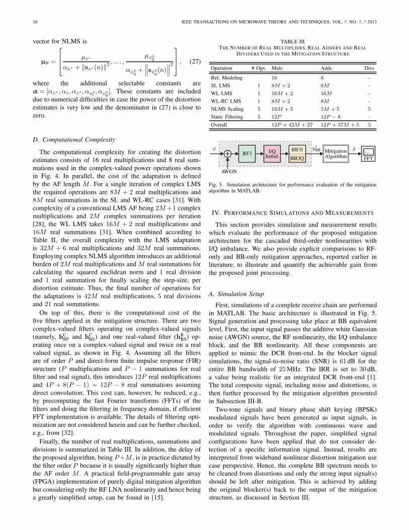
Fig. 5. Simulation architecture for performance evaluation of the mitigationalgorithm in MATLAB.

IV. PERFORMANCE SIMULATIONS AND MEASUREMENTS

This section provides simulation and measurement results

which evaluate the performance of the proposed mitigation

architecture for the cascaded third-order nonlinearities with

I/Q imbalance. We also provide explicit comparisons to RF-

only and BB-only mitigation approaches, reported earlier in

literature, to illustrate and quantify the achievable gain from

the proposed joint processing.

A. Simulation Setup

First, simulations of a complete receive chain are performed

in MATLAB. The basic architecture is illustrated in Fig. 5.

Signal generation and processing take place at BB equivalent

level. First, the input signal passes the additive white Gaussian

noise (AWGN) source, the RF nonlinearity, the I/Q imbalance

block, and the BB nonlinearity. All these components are

applied to mimic the DCR front-end. In the blocker signal

simulations, the signal-to-noise ratio (SNR) is 61 dB for the

entire BB bandwidth of 25MHz. The IRR is set to 30 dB,

a value being realistic for an integrated DCR front-end [1].

The total composite signal, including noise and distortions, is

then further processed by the mitigation algorithm presented

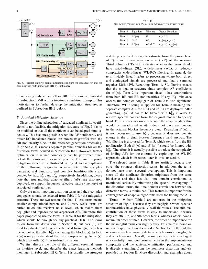
in Subsection III-B.

Two-tone signals and binary phase shift keying (BPSK)

modulated signals have been generated as input signals, in

order to verify the algorithm with continuous wave and

modulated signals. Throughout the paper, simplified signal

configurations have been applied that do not consider de-

tection of a specific information signal. Instead, results are

interpreted from wideband nonlinear distortion mitigation use

case perspective. Hence, the complete BB spectrum needs to

be cleaned from distortions and only the strong input signal(s)

should be left after mitigation. This is achieved by adding

the original blocker(s) back to the output of the mitigation

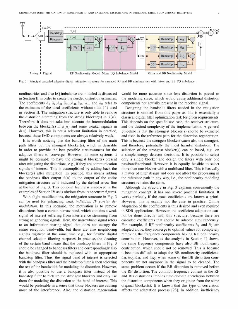
structure, as discussed in Section III.

GRIMM et al.: JOINT MITIGATION OF NONLINEAR RF AND BASEBAND DISTORTIONS IN WIDEBAND DIRECT-CONVERSION RECEIVERS 11

Single-tap complex AFs are used in the simulations, as also

the deployed circuit components models are memoryless. After

mitigation, block-wise FFT with 1024 points is applied to

analyze and illustrate the remaining nonlinear distortion. In the

following subsections, the last one of 29 FFT blocks is shown

in which the convergence of the coefficients is guaranteed.

As a figure of merit, the mitigation gain for the BPSK

case is computed as the reduction in average signal power

outside the original input (blocker) frequency band. Also

the mirror-image band is excluded from the mitigation gain

calculations as the focus is on the reduction in nonlinear

distortion power. For the two-tone case, average suppression

of nonlinear distortion components is used as a figure of merit,

meaning that average power decrease only on the specific fre-

quencies containing the nonlinear distortion is considered. For

measurements, this means the average power decrease on the

third-order distortion components whereas in the simulations

also the mirrors of these components are taken into account

as they also appear above the noise floor (see Fig. 7).

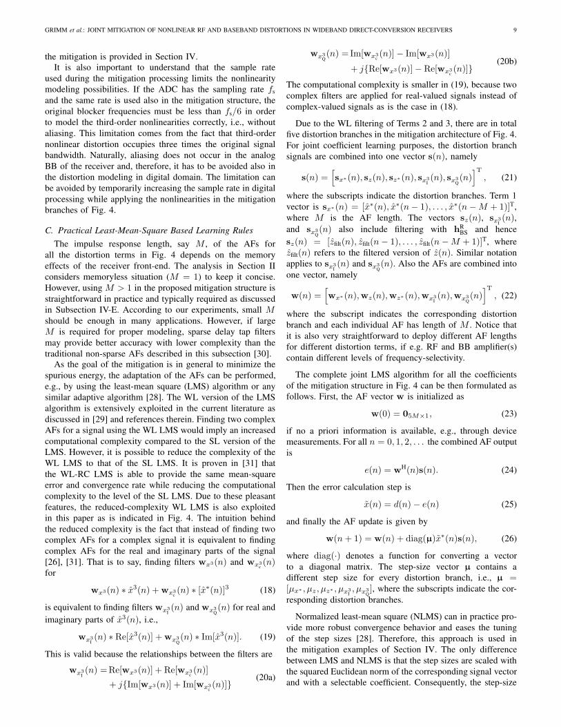
B. Two-tone Blocker Input

In order to demonstrate the most relevant distortion esti-

mates, the power levels of Terms 1–6 (as listed in Table I)

are next studied by means of a two-tone simulation. To keep

the illustration simple, mirror images are not included in

this particular example. In order to visualize all terms with

respect to their power level, noise has been excluded in this

particular simulation. Fig. 6a depicts the distortion estimates

for dominating RF nonlinearity, i.e., having |a2| > |a4|. Vector

a in the caption of Fig. 6 is defined as a = [a1, a2, a3, a4],where a3 = a3I = a3Q and similarly for a4. The applied pa-

rameters correspond to the ones defined in Table IV. In Fig. 6,

Term 2 is stemming from both the RF and BB distortion

whereas the other terms are due to the BB nonlinearity only,

as discussed in Sections II and III. Variable x (Term 1) depicts

the BB spectrum of the filtered blocker signal that serves as

an input for the reference nonlinearity. It is apparent that the

Terms 2 and 3 are the most significant ones in this case. It

is sufficient to consider common spectral content of multiple

terms by only one term, as the AF adapts the term to the total

distortion at these frequencies. Thus, only those distortions

of higher-order terms need to be considered that have not

been covered by lower-order terms. However, in this case,

frequency components added by Terms 4–6 are 80 dB or more

below the input power level and, therefore, likely to be masked

by noise in practice. In addition, SNR of a typical ADC is

approx. 60–80 dB depending on its resolution, hence making

all terms below −80 dBFS to disappear below quantization

noise. Fig. 6b illustrates then the power levels for dominating

BB nonlinearity case, i.e., |a2| < |a4|. The same parameters

values from Table I are used, but the gain and input-referred

third-order intercept point (IIP3) of the RF stage are applied

now for the BB and vice versa in order to make the BB

dominating. In Fig. 6b, Term 2 and Term 3 are almost equally

strong, but still these two terms are the most significant. The

observations support the analysis in Sections II and III, and

are assumed to be valid for practical values of RF and BB

nonlinearities.

Term 6

Term 5

Term 4

Term 3

Term 2

Term 1

Rel

ativ

eP

ow

er(d

B)

Baseband Frequency (MHz)−10 −5 0 5 10

−200

−150

−100

−50

0

50

(a)

Term 6

Term 5

Term 4

Term 3

Term 2

Term 1

Rel

ativ

eP

ow

er(d

B)

Baseband Frequency (MHz)−10 −5 0 5 10

−200

−150

−100

−50

0

50

(b)

Fig. 6. Power levels of distortion estimates with (a) dominating RF nonlin-earity a = [5.62,−(84351 + j74391), 3.16,−1588.7] and (b) dominatingBB nonlinearity a = [3.16,−1588.7, 5.62,−(84351 + j74391)]. Forsimplification, mirror terms are not visualized.

TABLE IVPARAMETERS OF THE TWO-TONE SIMULATION

IIP3 RF −10 dBm

GRF 15 dB

IIP3BB +6 dBm

GBB 10 dB

Pinput −30 dBm

a [5.62,−(84351 + j74391), 3.16,−1588.7]

gm 0.99}

IRR ≈ 30 dBφm 0.0628 = 3.6°

µ [1, 1, 0.01, 1, 1]

α [10−9, 10−8, 10−4, 10−9, 10−8]

The parameters for the actual performance simulations,

including also mirror effects, are summarized in Table IV,

where the coefficients of the nonlinearity models and the

I/Q imbalance coefficients are taken into account according

to (7), (13a), (13b), and (9). It is noteworthy that phase

distortions created by LNA and mixer are considered by

complex coefficients a2, k1, and k2. The coefficients a1 . . . a4have been computed based on practical values for gain and

IIP3 of the RF and BB amplifiers [12].

Fig. 7a illustrates the BB spectrum with a two-tone in-

put before and after proposed mitigation. With the two-

tone input, 16 signal components are created in total due

to the receiver nonlinearities and I/Q imbalance. The mirror

images appear 30 dB below the original tones, whereas the

strongest distortion components due to the nonlineaties are

36 dB below the original tones. First, the two-tone signal

12 IEEE TRANSACTIONS ON MICROWAVE THEORY AND TECHNIQUES, VOL. ?, NO. ?, ? 2013

After Mitigation

Before MitigationR

elat

ive

Pow

er(d

B)

Baseband Frequency (MHz)

BB Distortions(Mirror+TT)

Mirror-Frequency

BB Distortions

RF+BB Distortions

TT Input

−10 −5 0 5 10−100

−90

−80

−70

−60

−50

−40

−30

−20

−10

0

(a)

After Mitigation

Before Mitigation

Rel

ativ

eP

ow

er(d

B)

Baseband Frequency (MHz)

BB Distortions(Mirror+TT)

Mirror-Frequency

BB Distortions

RF+BB Distortions

TT Input

−10 −5 0 5 10−100

−90

−80

−70

−60

−50

−40

−30

−20

−10

0

(b)

After Mitigation

Before Mitigation

Rel

ativ

eP

ow

er(d

B)

Baseband Frequency (MHz)

BB Distortions(Mirror+TT)

Mirror-Frequency

BB Distortions

RF+BB Distortions

TT Input

−10 −5 0 5 10−100

−90

−80

−70

−60

−50

−40

−30

−20

−10

0

(c)

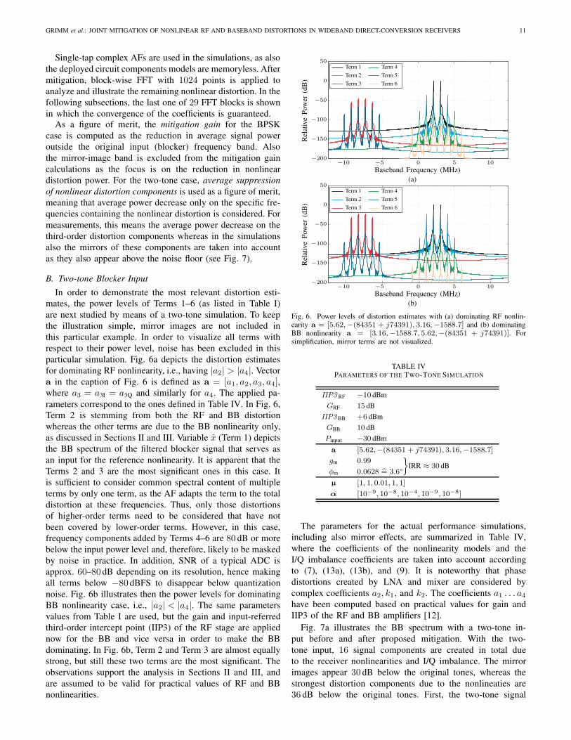
Fig. 7. Simulation results with two-tone input and mitigation with (a) theproposed cascaded model, (b) RF-only model, and (c) BB-only model.

is distorted by the RF amplifier, causing IMDs nearby the

original baseband-equivalent frequency at 2.6MHz (center of

the two tones). Second, mirror components of the original

tones and the RF distortion components appear due to down-

converting mixer I/Q mismatches. Third, the original tones

plus the RF distortions and their respective mirror components

are all further distorted by the BB I and Q nonlinearities. This

creates distortions at the third harmonic zone of the original

signal on the left side of the spectrum around −7.8MHz and

adds distortion around the original tones. In addition, the BB

nonlinearity causes harmonics and IMD originating from the

mirror components which then appear as low-power tones

around +7.8MHz. Furthermore, the BB distortions can have

respective mirror components, if there is I/Q imbalance in the

BB branches, although these components are very likely to

remain below the noise floor in practice. In fact, the mirror

components of the main RF and BB distortions are mitigated

with the WL filters in the proposed structure if they do appear.

Furthermore, AM/PM distortion caused at the RF amplifier

[24] and phase mismatch introduced by the mixer are taken

× 103

× 103

Samples

Im[x3]

z∗x∗

Re[x3]z

LSNLMS

0 1 2 3 4 5 6 7 8 9 10

0 1 2 3 4 5 6 7 8 9 10

0

5

10

15

0

10

20

30

40

50

60

0

0.005

0.01

0.015

0.02

0.025

0.03

0.035

0.04

0

5

10

15

0

50

100

150

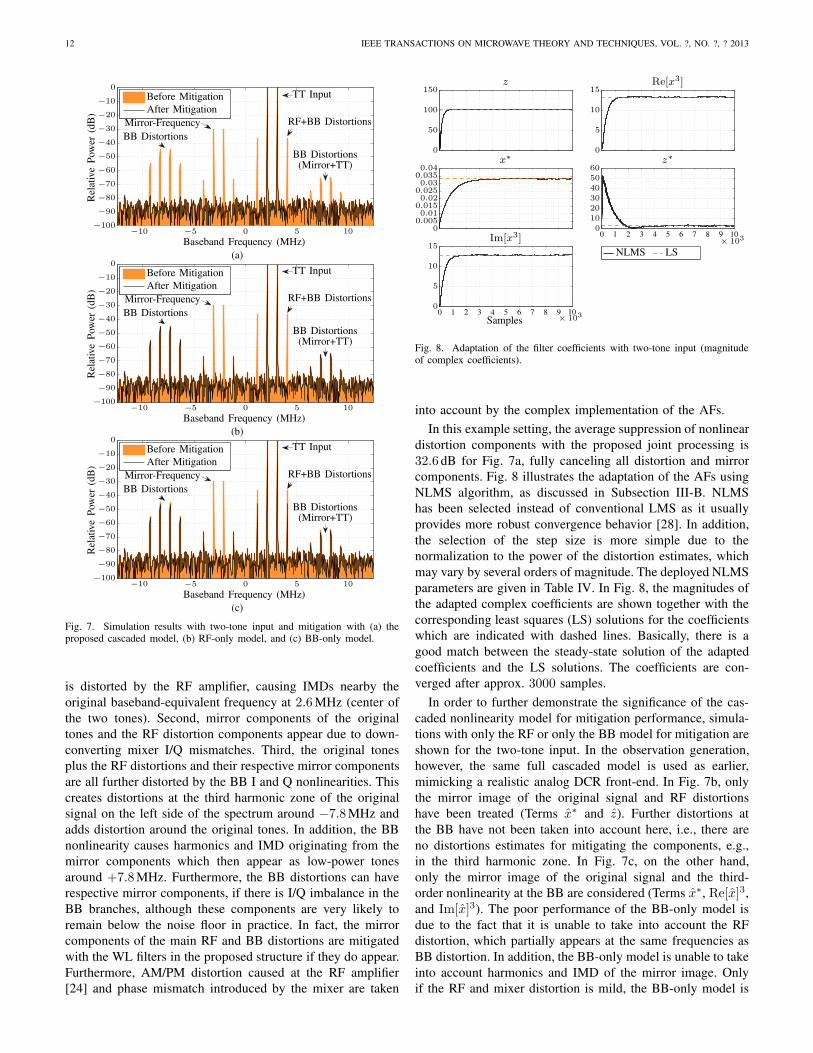
Fig. 8. Adaptation of the filter coefficients with two-tone input (magnitudeof complex coefficients).

into account by the complex implementation of the AFs.

In this example setting, the average suppression of nonlinear

distortion components with the proposed joint processing is

32.6 dB for Fig. 7a, fully canceling all distortion and mirror

components. Fig. 8 illustrates the adaptation of the AFs using

NLMS algorithm, as discussed in Subsection III-B. NLMS

has been selected instead of conventional LMS as it usually

provides more robust convergence behavior [28]. In addition,

the selection of the step size is more simple due to the

normalization to the power of the distortion estimates, which

may vary by several orders of magnitude. The deployed NLMS

parameters are given in Table IV. In Fig. 8, the magnitudes of

the adapted complex coefficients are shown together with the

corresponding least squares (LS) solutions for the coefficients

which are indicated with dashed lines. Basically, there is a

good match between the steady-state solution of the adapted

coefficients and the LS solutions. The coefficients are con-

verged after approx. 3000 samples.

In order to further demonstrate the significance of the cas-

caded nonlinearity model for mitigation performance, simula-

tions with only the RF or only the BB model for mitigation are

shown for the two-tone input. In the observation generation,

however, the same full cascaded model is used as earlier,

mimicking a realistic analog DCR front-end. In Fig. 7b, only

the mirror image of the original signal and RF distortions

have been treated (Terms x∗ and z). Further distortions at

the BB have not been taken into account here, i.e., there are

no distortions estimates for mitigating the components, e.g.,

in the third harmonic zone. In Fig. 7c, on the other hand,

only the mirror image of the original signal and the third-

order nonlinearity at the BB are considered (Terms x∗, Re[x]3,

and Im[x]3). The poor performance of the BB-only model is

due to the fact that it is unable to take into account the RF

distortion, which partially appears at the same frequencies as

BB distortion. In addition, the BB-only model is unable to take

into account harmonics and IMD of the mirror image. Only

if the RF and mixer distortion is mild, the BB-only model is

GRIMM et al.: JOINT MITIGATION OF NONLINEAR RF AND BASEBAND DISTORTIONS IN WIDEBAND DIRECT-CONVERSION RECEIVERS 13

(dB

)Ideal

Cascaded

BB-only

RF-only

−50 −48 −46 −44 −42 −40 −38 −36 −34 −32 −300

5

10

15

20

25

30

35

(a)

(dB

)

Input Power (dBm)−50 −48 −46 −44 −42 −40 −380

5

10

15

20

25

30

35

(b)

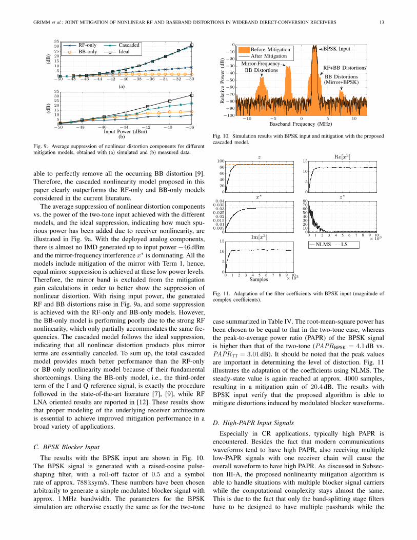
Fig. 9. Average suppression of nonlinear distortion components for differentmitigation models, obtained with (a) simulated and (b) measured data.

able to perfectly remove all the occurring BB distortion [9].

Therefore, the cascaded nonlinearity model proposed in this

paper clearly outperforms the RF-only and BB-only models

considered in the current literature.

The average suppression of nonlinear distortion components

vs. the power of the two-tone input achieved with the different

models, and the ideal suppression, indicating how much spu-

rious power has been added due to receiver nonlinearity, are

illustrated in Fig. 9a. With the deployed analog components,

there is almost no IMD generated up to input power −46 dBm

and the mirror-frequency interference x∗ is dominating. All the

models include mitigation of the mirror with Term 1, hence,

equal mirror suppression is achieved at these low power levels.

Therefore, the mirror band is excluded from the mitigation

gain calculations in order to better show the suppression of

nonlinear distortion. With rising input power, the generated

RF and BB distortions raise in Fig. 9a, and some suppression

is achieved with the RF-only and BB-only models. However,

the BB-only model is performing poorly due to the strong RF

nonlinearity, which only partially accommodates the same fre-

quencies. The cascaded model follows the ideal suppression,

indicating that all nonlinear distortion products plus mirror

terms are essentially canceled. To sum up, the total cascaded

model provides much better performance than the RF-only

or BB-only nonlinearity model because of their fundamental

shortcomings. Using the BB-only model, i.e., the third-order

term of the I and Q reference signal, is exactly the procedure

followed in the state-of-the-art literature [7], [9], while RF

LNA oriented results are reported in [12]. These results show

that proper modeling of the underlying receiver architecture

is essential to achieve improved mitigation performance in a

broad variety of applications.

C. BPSK Blocker Input

The results with the BPSK input are shown in Fig. 10.

The BPSK signal is generated with a raised-cosine pulse-

shaping filter, with a roll-off factor of 0.5 and a symbol

rate of approx. 788 ksym/s. These numbers have been chosen

arbitrarily to generate a simple modulated blocker signal with

approx. 1MHz bandwidth. The parameters for the BPSK

simulation are otherwise exactly the same as for the two-tone

After Mitigation

Before Mitigation

Rel

ativ

eP

ow

er(d

B)

Baseband Frequency (MHz)

BB Distortions(Mirror+BPSK)

Mirror-Frequency

BB Distortions RF+BB Distortions

BPSK Input

−10 −5 0 5 10−100

−90

−80

−70

−60

−50

−40

−30

−20

−10

0

Fig. 10. Simulation results with BPSK input and mitigation with the proposedcascaded model.

× 103

× 103

Samples

Im[x3]

z∗x∗

Re[x3]z

LSNLMS

0 1 2 3 4 5 6 7 8 9 10

0 1 2 3 4 5 6 7 8 9 10

0

5

10

15

0

10

20

30

40

50

60

70

80

0

0.005

0.01

0.015

0.02

0.025

0.03

0.035

0.04

0

5

10

15

0

20

40

60

80

100

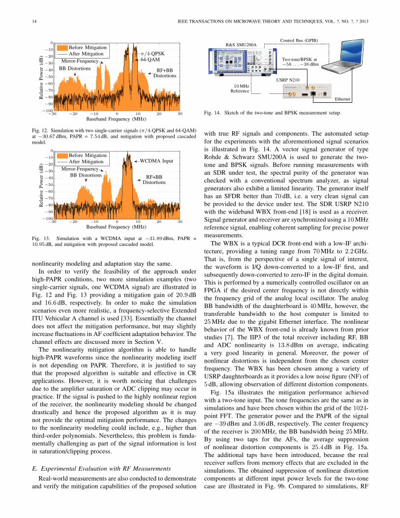
Fig. 11. Adaptation of the filter coefficients with BPSK input (magnitude ofcomplex coefficients).

case summarized in Table IV. The root-mean-square power has

been chosen to be equal to that in the two-tone case, whereas

the peak-to-average power ratio (PAPR) of the BPSK signal

is higher than that of the two-tone (PAPRBPSK = 4.1 dB vs.

PAPRTT = 3.01 dB). It should be noted that the peak values

are important in determining the level of distortion. Fig. 11

illustrates the adaptation of the coefficients using NLMS. The

steady-state value is again reached at approx. 4000 samples,

resulting in a mitigation gain of 20.4 dB. The results with

BPSK input verify that the proposed algorithm is able to

mitigate distortions induced by modulated blocker waveforms.

D. High-PAPR Input Signals

Especially in CR applications, typically high PAPR is

encountered. Besides the fact that modern communications

waveforms tend to have high PAPR, also receiving multiple

low-PAPR signals with one receiver chain will cause the

overall waveform to have high PAPR. As discussed in Subsec-

tion III-A, the proposed nonlinearity mitigation algorithm is

able to handle situations with multiple blocker signal carriers

while the computational complexity stays almost the same.

This is due to the fact that only the band-splitting stage filters

have to be designed to have multiple passbands while the

14 IEEE TRANSACTIONS ON MICROWAVE THEORY AND TECHNIQUES, VOL. ?, NO. ?, ? 2013

After Mitigation

Before Mitigation

Rel

ativ

eP

ow

er(d

B)

Baseband Frequency (MHz)

Mirror-Frequency

BB Distortions RF+BBDistortions

π/4-QPSK

64-QAM

−30 −20 −10 0 10 20 30−100

−90

−80

−70

−60

−50

−40

−30

−20

−10

0

Fig. 12. Simulation with two single-carrier signals (π/4-QPSK and 64-QAM)at −30.67 dBm, PAPR = 7.54 dB, and mitigation with proposed cascadedmodel.

After Mitigation

Before Mitigation

Rel

ativ

eP

ow

er(d

B)

Baseband Frequency (MHz)

Mirror-Frequency

BB Distortions RF+BBDistortions

WCDMA Input

−30 −20 −10 0 10 20 30−100

−90

−80

−70

−60

−50

−40

−30

−20

−10

0

Fig. 13. Simulation with a WCDMA input at −31.89 dBm, PAPR =10.95 dB, and mitigation with proposed cascaded model.

nonlinearity modeling and adaptation stay the same.

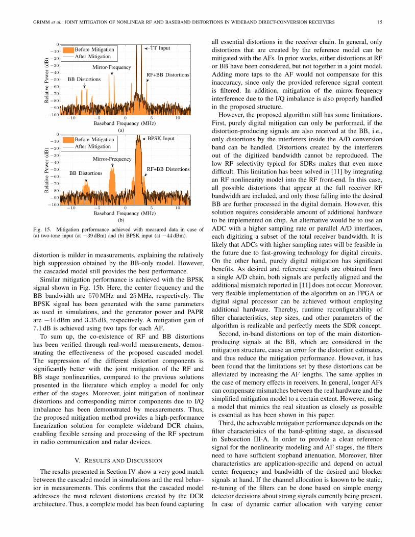
In order to verify the feasibility of the approach under

high-PAPR conditions, two more simulation examples (two

single-carrier signals, one WCDMA signal) are illustrated in

Fig. 12 and Fig. 13 providing a mitigation gain of 20.9 dB

and 16.6 dB, respectively. In order to make the simulation

scenarios even more realistic, a frequency-selective Extended

ITU Vehicular A channel is used [33]. Essentially the channel

does not affect the mitigation performance, but may slightly

increase fluctuations in AF coefficient adaptation behavior. The

channel effects are discussed more in Section V.

The nonlinearity mitigation algorithm is able to handle

high-PAPR waveforms since the nonlinearity modeling itself

is not depending on PAPR. Therefore, it is justified to say

that the proposed algorithm is suitable and effective in CR

applications. However, it is worth noticing that challenges

due to the amplifier saturation or ADC clipping may occur in

practice. If the signal is pushed to the highly nonlinear region

of the receiver, the nonlinearity modeling should be changed

drastically and hence the proposed algorithm as it is may

not provide the optimal mitigation performance. The changes

to the nonlinearity modeling could include, e.g., higher than

third-order polynomials. Nevertheless, this problem is funda-

mentally challenging as part of the signal information is lost

in saturation/clipping process.

E. Experimental Evaluation with RF Measurements

Real-world measurements are also conducted to demonstrate

and verify the mitigation capabilities of the proposed solution

−58 . . .−38 dBm

10MHz

Control Bus (GPIB)

Ethernet

R&S SMU200A

Reference

Two-tone/BPSK at

USRP N210

Fig. 14. Sketch of the two-tone and BPSK measurement setup.

with true RF signals and components. The automated setup

for the experiments with the aforementioned signal scenarios

is illustrated in Fig. 14. A vector signal generator of type

Rohde & Schwarz SMU200A is used to generate the two-

tone and BPSK signals. Before running measurements with

an SDR under test, the spectral purity of the generator was

checked with a conventional spectrum analyzer, as signal

generators also exhibit a limited linearity. The generator itself

has an SFDR better than 70 dB, i.e. a very clean signal can

be provided to the device under test. The SDR USRP N210

with the wideband WBX front-end [18] is used as a receiver.

Signal generator and receiver are synchronized using a 10MHz

reference signal, enabling coherent sampling for precise power

measurements.

The WBX is a typical DCR front-end with a low-IF archi-

tecture, providing a tuning range from 70MHz to 2.2GHz.

That is, from the perspective of a single signal of interest,

the waveform is I/Q down-converted to a low-IF first, and

subsequently down-converted to zero-IF in the digital domain.

This is performed by a numerically controlled oscillator on an

FPGA if the desired center frequency is not directly within

the frequency grid of the analog local oscillator. The analog

BB bandwidth of the daughterboard is 40MHz, however, the

transferable bandwidth to the host computer is limited to

25MHz due to the gigabit Ethernet interface. The nonlinear

behavior of the WBX front-end is already known from prior

studies [7]. The IIP3 of the total receiver including RF, BB

and ADC nonlinearity is 13.8 dBm on average, indicating

a very good linearity in general. Moreover, the power of

nonlinear distortions is independent from the chosen center

frequency. The WBX has been chosen among a variety of

USRP daughterboards as it provides a low noise figure (NF) of

5 dB, allowing observation of different distortion components.

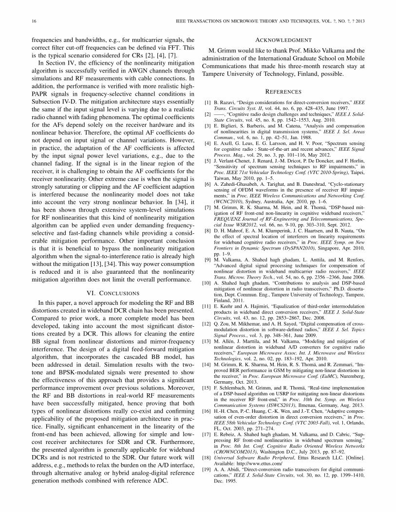
Fig. 15a illustrates the mitigation performance achieved

with a two-tone input. The tone frequencies are the same as in

simulations and have been chosen within the grid of the 1024-

point FFT. The generator power and the PAPR of the signal

are −39 dBm and 3.06 dB, respectively. The center frequency

of the receiver is 200MHz, the BB bandwidth being 25MHz.

By using two taps for the AFs, the average suppression

of nonlinear distortion components is 25.4 dB in Fig. 15a.

The additional taps have been introduced, because the real

receiver suffers from memory effects that are excluded in the

simulations. The obtained suppression of nonlinear distortion

components at different input power levels for the two-tone

case are illustrated in Fig. 9b. Compared to simulations, RF

GRIMM et al.: JOINT MITIGATION OF NONLINEAR RF AND BASEBAND DISTORTIONS IN WIDEBAND DIRECT-CONVERSION RECEIVERS 15

After Mitigation

Before MitigationR

elat

ive

Pow

er(d

B)

Baseband Frequency (MHz)

Mirror-Frequency

BB DistortionsRF+BB Distortions

TT Input

−10 −5 0 5 10−100

−90

−80

−70

−60

−50

−40

−30

−20

−10

0

(a)

After Mitigation

Before Mitigation

Rel

ativ

eP

ow

er(d

B)

Baseband Frequency (MHz)

Mirror-Frequency

BB DistortionsRF+BB Distortions

BPSK Input

−10 −5 0 5 10−100

−90

−80

−70

−60

−50

−40

−30

−20

−10

0

(b)

Fig. 15. Mitigation performance achieved with measured data in case of(a) two-tone input (at −39 dBm) and (b) BPSK input (at −44 dBm).

distortion is milder in measurements, explaining the relatively

high suppression obtained by the BB-only model. However,

the cascaded model still provides the best performance.

Similar mitigation performance is achieved with the BPSK

signal shown in Fig. 15b. Here, the center frequency and the

BB bandwidth are 570MHz and 25MHz, respectively. The

BPSK signal has been generated with the same parameters

as used in simulations, and the generator power and PAPR

are −44 dBm and 3.35 dB, respectively. A mitigation gain of

7.1 dB is achieved using two taps for each AF.

To sum up, the co-existence of RF and BB distortions

has been verified through real-world measurements, demon-

strating the effectiveness of the proposed cascaded model.

The suppression of the different distortion components is

significantly better with the joint mitigation of the RF and

BB stage nonlinearities, compared to the previous solutions

presented in the literature which employ a model for only

either of the stages. Moreover, joint mitigation of nonlinear

distortions and corresponding mirror components due to I/Q

imbalance has been demonstrated by measurements. Thus,

the proposed mitigation method provides a high-performance

linearization solution for complete wideband DCR chains,

enabling flexible sensing and processing of the RF spectrum

in radio communication and radar devices.

V. RESULTS AND DISCUSSION

The results presented in Section IV show a very good match

between the cascaded model in simulations and the real behav-

ior in measurements. This confirms that the cascaded model

addresses the most relevant distortions created by the DCR

architecture. Thus, a complete model has been found capturing

all essential distortions in the receiver chain. In general, only

distortions that are created by the reference model can be

mitigated with the AFs. In prior works, either distortions at RF

or BB have been considered, but not together in a joint model.

Adding more taps to the AF would not compensate for this

inaccuracy, since only the provided reference signal content

is filtered. In addition, mitigation of the mirror-frequency

interference due to the I/Q imbalance is also properly handled

in the proposed structure.

However, the proposed algorithm still has some limitations.

First, purely digital mitigation can only be performed, if the

distortion-producing signals are also received at the BB, i.e.,

only distortions by the interferers inside the A/D conversion

band can be handled. Distortions created by the interferers

out of the digitized bandwidth cannot be reproduced. The

low RF selectivity typical for SDRs makes that even more

difficult. This limitation has been solved in [11] by integrating

an RF nonlinearity model into the RF front-end. In this case,

all possible distortions that appear at the full receiver RF

bandwidth are included, and only those falling into the desired

BB are further processed in the digital domain. However, this

solution requires considerable amount of additional hardware

to be implemented on chip. An alternative would be to use an

ADC with a higher sampling rate or parallel A/D interfaces,

each digitizing a subset of the total receiver bandwidth. It is

likely that ADCs with higher sampling rates will be feasible in

the future due to fast-growing technology for digital circuits.

On the other hand, purely digital mitigation has significant

benefits. As desired and reference signals are obtained from

a single A/D chain, both signals are perfectly aligned and the

additional mismatch reported in [11] does not occur. Moreover,

very flexible implementation of the algorithm on an FPGA or

digital signal processor can be achieved without employing

additional hardware. Thereby, runtime reconfigurability of

filter characteristics, step sizes, and other parameters of the

algorithm is realizable and perfectly meets the SDR concept.

Second, in-band distortions on top of the main distortion-

producing signals at the BB, which are considered in the

mitigation structure, cause an error for the distortion estimates,

and thus reduce the mitigation performance. However, it has

been found that the limitations set by these distortions can be

alleviated by increasing the AF lengths. The same applies in

the case of memory effects in receivers. In general, longer AFs

can compensate mismatches between the real hardware and the

simplified mitigation model to a certain extent. However, using

a model that mimics the real situation as closely as possible

is essential as has been shown in this paper.

Third, the achievable mitigation performance depends on the

filter characteristics of the band-splitting stage, as discussed

in Subsection III-A. In order to provide a clean reference

signal for the nonlinearity modeling and AF stages, the filters

need to have sufficient stopband attenuation. Moreover, filter

characteristics are application-specific and depend on actual

center frequency and bandwidth of the desired and blocker

signals at hand. If the channel allocation is known to be static,

re-tuning of the filters can be done based on simple energy

detector decisions about strong signals currently being present.

In case of dynamic carrier allocation with varying center

16 IEEE TRANSACTIONS ON MICROWAVE THEORY AND TECHNIQUES, VOL. ?, NO. ?, ? 2013

frequencies and bandwidths, e.g., for multicarrier signals, the

correct filter cut-off frequencies can be defined via FFT. This

is the typical scenario considered for CRs [2], [4], [7].

In Section IV, the efficiency of the nonlinearity mitigation

algorithm is successfully verified in AWGN channels through

simulations and RF measurements with cable connections. In

addition, the performance is verified with more realistic high-

PAPR signals in frequency-selective channel conditions in

Subsection IV-D. The mitigation architecture stays essentially

the same if the input signal level is varying due to a realistic

radio channel with fading phenomena. The optimal coefficients

for the AFs depend solely on the receiver hardware and its

nonlinear behavior. Therefore, the optimal AF coefficients do

not depend on input signal or channel variations. However,

in practice, the adaptation of the AF coefficients is affected

by the input signal power level variations, e.g., due to the

channel fading. If the signal is in the linear region of the

receiver, it is challenging to obtain the AF coefficients for the

receiver nonlinearity. Other extreme case is when the signal is

strongly saturating or clipping and the AF coefficient adaption

is interfered because the nonlinearity model does not take

into account the very strong nonlinear behavior. In [34], it

has been shown through extensive system-level simulations

for RF nonlinearities that this kind of nonlinearity mitigation

algorithm can be applied even under demanding frequency-

selective and fast-fading channels while providing a consid-

erable mitigation performance. Other important conclusion

is that it is beneficial to bypass the nonlinearity mitigation

algorithm when the signal-to-interference ratio is already high

without the mitigation [13], [34]. This way power consumption

is reduced and it is also guaranteed that the nonlinearity

mitigation algorithm does not limit the overall performance.

VI. CONCLUSIONS

In this paper, a novel approach for modeling the RF and BB

distortions created in wideband DCR chain has been presented.

Compared to prior work, a more complete model has been

developed, taking into account the most significant distor-

tions created by a DCR. This allows for cleaning the entire

BB signal from nonlinear distortions and mirror-frequency

interference. The design of a digital feed-forward mitigation

algorithm, that incorporates the cascaded BB model, has

been addressed in detail. Simulation results with the two-

tone and BPSK-modulated signals were presented to show

the effectiveness of this approach that provides a significant

performance improvement over previous solutions. Moreover,

the RF and BB distortions in real-world RF measurements

have been successfully mitigated, hence proving that both

types of nonlinear distortions really co-exist and confirming

applicability of the proposed mitigation architecture in prac-

tice. Finally, significant enhancement in the linearity of the

front-end has been achieved, allowing for simple and low-

cost receiver architectures for SDR and CR. Furthermore,

the presented algorithm is generally applicable for wideband

DCRs and is not restricted to the SDR. Our future work will

address, e.g., methods to relax the burden on the A/D interface,

through alternative analog or hybrid analog-digital reference

generation methods combined with reference ADC.

ACKNOWLEDGMENT

M. Grimm would like to thank Prof. Mikko Valkama and the

administration of the International Graduate School on Mobile

Communications that made his three-month research stay at

Tampere University of Technology, Finland, possible.

REFERENCES

[1] B. Razavi, “Design considerations for direct-conversion receivers,” IEEE

Trans. Circuits Syst. II, vol. 44, no. 6, pp. 428–435, June 1997.

[2] ——, “Cognitive radio design challenges and techniques,” IEEE J. Solid-State Circuits, vol. 45, no. 8, pp. 1542–1553, Aug. 2010.

[3] E. Biglieri, S. Barberis, and M. Catena, “Analysis and compensationof nonlinearities in digital transmission systems,” IEEE J. Sel. Areas

Commun., vol. 6, no. 1, pp. 42–51, Jan. 1988.[4] E. Axell, G. Leus, E. G. Larsson, and H. V. Poor, “Spectrum sensing

for cognitive radio : State-of-the-art and recent advances,” IEEE Signal

Process. Mag., vol. 29, no. 3, pp. 101–116, May 2012.

[5] J. Verlant-Chenet, J. Renard, J.-M. Dricot, P. De Doncker, and F. Horlin,“Sensitivity of spectrum sensing techniques to RF impairments,” inProc. IEEE 71st Vehicular Technology Conf. (VTC 2010-Spring), Taipei,Taiwan, May 2010, pp. 1–5.

[6] A. Zahedi-Ghasabeh, A. Tarighat, and B. Daneshrad, “Cyclo-stationarysensing of OFDM waveforms in the presence of receiver RF impair-ments,” in Proc. IEEE Wireless Communications and Networking Conf.

(WCNC2010), Sydney, Australia, Apr. 2010, pp. 1–6.

[7] M. Grimm, R. K. Sharma, M. Hein, and R. Thomä, “DSP-based mit-igation of RF front-end non-linearity in cognitive wideband receivers,”FREQUENZ Journal of RF-Engineering and Telecommunications, Spe-

cial Issue WSR2012, vol. 66, no. 9-10, pp. 303–310, Sept. 2012.

[8] D. H. Mahrof, E. A. M. Klumperink, J. C. Haartsen, and B. Nauta, “Onthe effect of spectral location of interferers on linearity requirementsfor wideband cognitive radio receivers,” in Proc. IEEE Symp. on New

Frontiers in Dynamic Spectrum (DySPAN2010), Singapore, Apr. 2010,pp. 1–9.

[9] M. Valkama, A. Shahed hagh ghadam, L. Anttila, and M. Renfors,“Advanced digital signal processing techniques for compensation ofnonlinear distortion in wideband multicarrier radio receivers,” IEEE

Trans. Microw. Theory Tech., vol. 54, no. 6, pp. 2356 –2366, June 2006.[10] A. Shahed hagh ghadam, “Contributions to analysis and DSP-based

mitigation of nonlinear distortion in radio transceivers,” Ph.D. disserta-tion, Dept. Commun. Eng., Tampere University of Technology, Tampere,Finland, 2011.

[11] E. Keehr and A. Hajimiri, “Equalization of third-order intermodulationproducts in wideband direct conversion receivers,” IEEE J. Solid-State

Circuits, vol. 43, no. 12, pp. 2853–2867, Dec. 2008.

[12] Q. Zou, M. Mikhemar, and A. H. Sayed, “Digital compensation of cross-modulation distortion in software-defined radios,” IEEE J. Sel. Topics

Signal Process., vol. 3, pp. 348–361, June 2009.

[13] M. Allén, J. Marttila, and M. Valkama, “Modeling and mitigation ofnonlinear distortion in wideband A/D converters for cognitive radioreceivers,” European Microwave Assoc. Int. J. Microwave and WirelessTechnologies, vol. 2, no. 02, pp. 183–192, Apr. 2010.

[14] M. Grimm, R. K. Sharma, M. Hein, R. S. Thomä, and R. Zemmari, “Im-proved BER performance in GSM by mitigating non-linear distortions inthe receiver,” in Proc. European Microwave Conf. (EuMC), Nuremberg,Germany, Oct. 2013.

[15] F. Schlembach, M. Grimm, and R. Thomä, “Real-time implementationof a DSP-based algorithm on USRP for mitigating non-linear distortionsin the receiver RF front-end,” in Proc. 10th Int. Symp. on WirelessCommunication Systems (ISWCS2013), Ilmenau, Germany, Aug. 2013.

[16] H.-H. Chen, P.-C. Huang, C.-K. Wen, and J.-T. Chen, “Adaptive compen-sation of even-order distortion in direct conversion receivers,” in Proc.

IEEE 58th Vehicular Technology Conf. (VTC 2003-Fall), vol. 1, Orlando,FL, Oct. 2003, pp. 271–274.

[17] E. Rebeiz, A. Shahed hagh ghadam, M. Valkama, and D. Cabric, “Sup-pressing RF front-end nonlinearities in wideband spectrum sensing,”in Proc. 8th Int. Conf. Cognitive Radio Oriented Wireless Networks(CROWNCOM2013), Washington D.C., July 2013, pp. 87–92.

[18] Universal Software Radio Peripheral, Ettus Research LLC. [Online].Available: http://www.ettus.com/

[19] A. A. Abidi, “Direct-conversion radio transceivers for digital communi-cations,” IEEE J. Solid-State Circuits, vol. 30, no. 12, pp. 1399–1410,Dec. 1995.

GRIMM et al.: JOINT MITIGATION OF NONLINEAR RF AND BASEBAND DISTORTIONS IN WIDEBAND DIRECT-CONVERSION RECEIVERS 17

[20] A. B. Carlson, P. B. Crilly, and J. C. Rutledge, Communication Systems:

An Introduction to Signals and Noise in Electrical Communication,4th ed. New York: McGraw-Hill, 2001, pp. 143–147.

[21] D. R. Morgan, Z. Ma, J. Kim, M. G. Zierdt, and J. Pastalan, “Ageneralized memory polynomial model for digital predistortion of RFpower amplifiers,” IEEE Trans. Signal Process., vol. 54, no. 10, pp.3852–3860, Oct. 2006.

[22] S. C. Blaakmeer, E. A. M. Klumperink, D. M. W. Leenaerts, andB. Nauta, “Wideband balun-LNA with simultaneous output balancing,noise-canceling and distortion-canceling,” IEEE J. Solid-State Circuits,vol. 43, no. 6, pp. 1341–1350, June 2008.

[23] K. Kivekäs, A. Pärssinen, and K. A. I. Halonen, “Characterization ofIIP2 and DC-offsets in transconductance mixers,” IEEE Trans. Circuits

Syst. II, vol. 48, no. 11, pp. 1028–1038, Nov. 2001.[24] P. B. Kenington, High-Linearity RF Amplifier Design. Norwood, MA:

Artech House, 2000, pp. 74–77.[25] L. Anttila, M. Valkama, and M. Renfors, “Circularity-based I/Q im-

balance compensation in wideband direct-conversion receivers,” IEEETrans. Veh. Technol., vol. 57, no. 4, pp. 2099–2113, July 2008.

[26] L. Anttila, “Digital front-end signal processing with widely-linear signalmodels in radio devices,” Ph.D. dissertation, Dept. Commun. Eng.,Tampere University of Technology, Tampere, Finland, 2011.

[27] J. L. Karki, “Designing for low distortion with high-speed op amps,”Texas Instruments Analog Applicat. J., pp. 25–33, July 2001. [Online].Available: http://www.ti.com/lit/an/slyt133/slyt133.pdf

[28] S. Haykin, Adaptive Filter Theory, 4th ed. Upper Saddle river, NJ:Prentice Hall, 2002, pp. 231–341.

[29] T. Adali, H. Li, and R. Aloysius, “On properties of the widely linearMSE filter and its LMS implementation,” in Proc. 43rd Annu. Conf.Information Sciences and Systems (CISS2009), Baltimore, MD, Mar.2009, pp. 876–881.

[30] H. Ku and J. S. Kenney, “Behavioral modeling of nonlinear RF poweramplifiers considering memory effects,” IEEE Trans. Microw. Theory

Tech., vol. 51, no. 12, pp. 2495–2504, Dec. 2003.[31] F. G. A. Neto, V. H. Nascimento, and M. T. M. Silva, “Reduced-

complexity widely linear adaptive estimation,” in Proc. 7th Int. Symp.Wireless Communication Systems (ISWCS2010), York, United Kingdom,Sept. 2010, pp. 399–403.

[32] R. Meyer, R. Reng, and K. Schwarz, “Convolution algorithms on DSPprocessors,” in Int. Conf. Acoustics, Speech, and Signal Process., vol. 3,Toronto, Canada, Apr. 1991, pp. 2193–2196.

[33] T. B. Sørensen, P. E. Mogensen, and F. Frederiksen, “Extension of theITU channel models for wideband (OFDM) systems,” in Proc. IEEE62nd Vehicular Technology Conf. (VTC 2005-Fall), vol. 1, Dallas, TX,Sept. 2005, pp. 392–396.

[34] D. Dupleich, M. Grimm, F. Schlembach, and R. S. Thomä, “Practicalaspects of a digital feedforward approach for mitigating non-lineardistortions in receivers,” in Proc. 11th Int. Conf. Telecommunications

in Modern Satellite, Cable and Broadcasting Services (TELSIKS2013),Niš, Serbia, Oct. 2013, pp. 170–177.

Michael Grimm was born in Weimar, Germany, onJanuary 7th, 1986. He received the Dipl.-Ing. degreein electrical engineering and information technologyfrom Ilmenau University of Technology, Germany, in2009.

He is currently with the Electronic Measure-ment Research Lab within the International Grad-uate School on Mobile Communications at IlmenauUniversity of Technology as a Researcher workingtowards the Dr.-Ing. degree (Ph.D.). His researchinterests include software defined and cognitive ra-

dio, RF impairment mitigation, mixed-signal circuit design, and FPGA-basedembedded signal processing.

Markus Allén (S’10) was born in Ypäjä, Finland, onOctober 28, 1985. He received the B.Sc. and M.Sc.degrees in signal processing and communicationsengineering from Tampere University of Technology,Finland, in 2008 and 2010, respectively.

He is currently with the Department of Electron-ics and Communications Engineering at TampereUniversity of Technology as a Researcher head-ing towards the Ph.D. degree. His current researchinterests include cognitive radios, analog-to-digitalconverters, receiver front-end nonlinearities and their

digital mitigation algorithms.

Jaakko Marttila (S’10) was born in Tampere, Fin-land, on March 30, 1982. He received the M.Sc.degree in signal processing and communicationsengineering from Tampere University of Technology(TUT), Tampere, Finland, in 2010.

He is currently working towards the Ph.D. degreeat TUT, Department of Electronics and Commu-nications Engineering as a Researcher. At present,his main research topic is quadrature sigma-deltaanalog-to-digital (AD) conversion. Generally, his re-search interests include AD techniques for software

defined and cognitive radios, and related interference mitigation algorithms.

Mikko Valkama (S’00, M’02) was born in Pirkkala,Finland, on November 27, 1975. He received theM.Sc. and Ph.D. degrees (both with honours) inelectrical engineering (EE) from Tampere Universityof Technology (TUT), Finland, in 2000 and 2001,respectively. In 2002 he received the Best Ph.D.Thesis award by the Finnish Academy of Scienceand Letters for his dissertation entitled "AdvancedI/Q signal processing for wideband receivers: Mod-els and algorithms".

In 2003, he was working as a visiting researcherwith the Communications Systems and Signal Processing Institute at SDSU,San Diego, CA. Currently, he is a Full Professor and Department ViceHead at the Department of Electronics and Communications Engineeringat TUT, Finland. He has been involved in organizing conferences, like theIEEE SPAWC’07 (Publications Chair) held in Helsinki, Finland. His generalresearch interests include communications signal processing, estimation anddetection techniques, signal processing algorithms for software defined flex-ible radios, cognitive radio, digital transmission techniques such as differentvariants of multicarrier modulation methods and OFDM, radio localizationmethods, and radio resource management for ad-hoc and mobile networks.

Reiner Thomä (M’92–SM’99–F’07) received theDipl.-Ing. (M.S.E.E.), Dr.-Ing. (Ph.D.E.E.), andthe Dr.-Ing. habil. degrees in electrical engineer-ing and information technology from TechnischeHochschule Ilmenau, Germany, in 1975, 1983, and1989, respectively.

From 1975 to 1988, he was a Research Associatein the fields of electronic circuits, measurement en-gineering, and digital signal processing at the sameuniversity. From 1988 to 1990, he was a ResearchEngineer at the Akademie der Wissenschaften der

DDR (Zentrum für Wissenschaftlichen Gerätebau). During this period hewas working in the field of radio surveillance. In 1991, he spent a three-month sabbatical leave at the University of Erlangen-Nürnberg (Lehrstuhlfür Nachrichtentechnik). Since 1992, he has been a Professor of electricalengineering (electronic measurement) at TU Ilmenau where he was theDirector of the Institute of Communications and Measurement Engineeringfrom 1999 until 2005. With his group, he has contributed to several Europeanand German research projects and clusters such as WINNER, PULSERS,EUWB, NEWCOM, COST 273, 2100, IC 1004, EASY-A, EASY-C. Currentlyhe is the speaker of the German nation-wide DFG-focus project UKoLOS,Ultra-Wideband Radio Technologies for Communications, Localization andSensor Applications (SPP 1202). His research interests include measurementand digital signal processing methods (correlation and spectral analysis,system identification, sensor arrays, compressive sensing, time-frequencyand cyclostationary signal analysis), their application in mobile radio andradar systems (multidimensional channel sounding, propagation measurementand parameter estimation, MIMO-, mm-wave-, and ultra-wideband radar),measurement-based performance evaluation of MIMO transmission systemsincluding over-the-air testing in virtual electromagnetic environments, andUWB sensor systems for object detection, tracking and imaging.

Prof. Thomä is a member of URSI (Comm. A), VDE/ITG. Since 1999 hehas been serving as chair of the IEEE-IM TC-13 on Measurement in Wirelessand Telecommunications. In 2007 he was awarded IEEE Fellow Member andreceived the Thuringian State Research Award for Applied Research both forcontributions to high-resolution multidimensional channel sounding.