Joint modeling of longitudinal and survival data · Joint modeling of longitudinal and survival...

Joint modeling of longitudinal and survival data

Joint modeling of longitudinal and survival

data

Yulia Marchenko

Executive Director of StatisticsStataCorp LP

2016 Nordic and Baltic Stata Users Group meeting

Yulia Marchenko (StataCorp) 1 / 55


Outline

Motivation

Joint analysis

New Stata commands for joint analysis

Joint analysis of the PANSS data

Models with more flexible latent associations

Summary

Future work

Acknowledgement

References



Motivation

Many studies collect both longitudinal (measurements) dataand survival-time data.

Longitudinal (or panel, or repeated-measures) data are data inwhich a response variable is measured at different time pointssuch as blood pressure, weight, or test scores measured overtime.

Survival-time or event history data record times until an eventof interest such as times until a heart attack or times untildeath from cancer.



Motivation

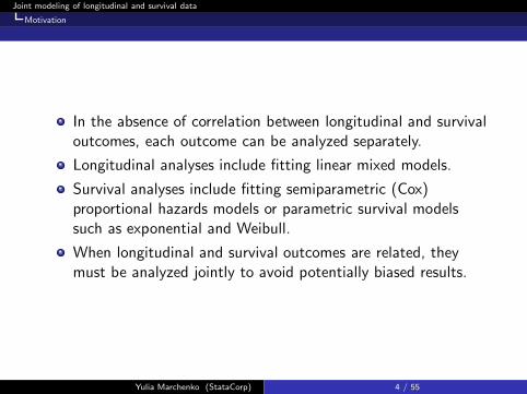
In the absence of correlation between longitudinal and survivaloutcomes, each outcome can be analyzed separately.

Longitudinal analyses include fitting linear mixed models.

Survival analyses include fitting semiparametric (Cox)proportional hazards models or parametric survival modelssuch as exponential and Weibull.

When longitudinal and survival outcomes are related, theymust be analyzed jointly to avoid potentially biased results.



Motivation

Joint analyses are useful to:

Account for informative dropout in the analysis of longitudinaldata;

Study effects of baseline covariates on longitudinal andsurvival outcomes; or

Study effects of time-dependent covariates on the survivaloutcome.

In this presentation, I will concentrate on the first two applications.



Motivation

PANSS study

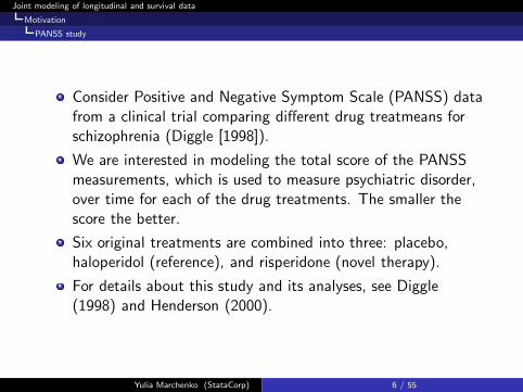
Consider Positive and Negative Symptom Scale (PANSS) datafrom a clinical trial comparing different drug treatmeans forschizophrenia (Diggle [1998]).

We are interested in modeling the total score of the PANSSmeasurements, which is used to measure psychiatric disorder,over time for each of the drug treatments. The smaller thescore the better.

Six original treatments are combined into three: placebo,haloperidol (reference), and risperidone (novel therapy).

For details about this study and its analyses, see Diggle(1998) and Henderson (2000).



Motivation

PANSS study

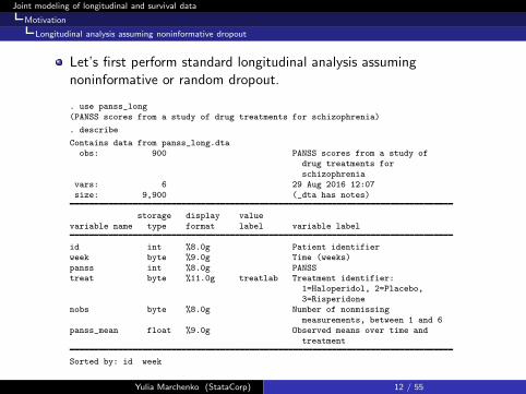
We consider a subset of the original data:

. use panss

(PANSS scores from a study of drug treatments for schizophrenia)

. describe

Contains data from panss.dtaobs: 150 PANSS scores from a study of

drug treatments forschizophrenia

vars: 11 29 Aug 2016 12:07

size: 3,150 (_dta has notes)

storage display valuevariable name type format label variable label

id int %8.0g Patient identifierpanss0 int %8.0g PANSS score at week 0

panss1 int %8.0g PANSS score at week 1panss2 int %8.0g PANSS score at week 2

panss4 int %8.0g PANSS score at week 4panss6 int %8.0g PANSS score at week 6panss8 int %8.0g PANSS score at week 8

treat byte %11.0g treatlab Treatment identifier:1=Haloperidol, 2=Placebo,

3=Risperidone



Motivation

PANSS study

nobs byte %8.0g Number of nonmissingmeasurements, between 1 and 6

droptime float %8.0g Imputed dropout time (weeks)infdrop byte %14.0g droplab Dropout indicator:

0=none or noninformative;1=informative

Sorted by: id

. notes

_dta:1. Subset of the data from a larger (confidential) randomized clinical trial

of drug treatments for schizophrenia2. Source:

http://www.lancaster.ac.uk/staff/diggle/APTS-data-sets/PANSS_short_data.t> xt

3. PANSS (Positive and Negative Symptom Scale)



Motivation

PANSS study

Listing of a subset of the data:

. list id panss* treat if inlist(id,1,2,3,10,19,24,30,42), sepby(nobs) noobs

id panss0 panss1 panss2 panss4 panss6 panss8 treat

1 91 . . . . . Haloperidol

2 72 . . . . . Placebo

3 108 110 . . . . Haloperidol

10 97 118 . . . . Placebo19 81 71 . . . . Risperidone

24 127 98 152 . . . Haloperidol

30 73 74 68 . . . Placebo42 75 92 117 . . . Risperidone



Motivation

PANSS study

Many patients withdrew from the study before completing themeasurement schedule—of the 150 subjects, only 68completed the study.

. misstable pattern panss*, freq bypattern

Missing-value patterns(1 means complete)

Pattern

Frequency 1 2 3 4 5

68 1 1 1 1 1

1:

16 1 1 1 1 02:

24 1 1 1 0 0

3:19 1 1 0 0 0

4:21 1 0 0 0 0

5:2 0 0 0 0 0

150

Variables are (1) panss1 (2) panss2 (3) panss4 (4) panss6 (5) panss8



Motivation

PANSS study

Over 40% of subjects specified the reason for dropout as“inadequate for response”, which suggests that the dropoutmay be informative.

. tabulate infdrop

Dropoutindicator Freq. Percent Cum.

None, noninf. 87 58.00 58.00Informative 63 42.00 100.00

Total 150 100.00



Motivation

Longitudinal analysis assuming noninformative dropout

Let’s first perform standard longitudinal analysis assumingnoninformative or random dropout.

. use panss_long

(PANSS scores from a study of drug treatments for schizophrenia)

. describe

Contains data from panss_long.dtaobs: 900 PANSS scores from a study of

drug treatments for

schizophreniavars: 6 29 Aug 2016 12:07

size: 9,900 (_dta has notes)

storage display value

variable name type format label variable label

id int %8.0g Patient identifierweek byte %9.0g Time (weeks)

panss int %8.0g PANSStreat byte %11.0g treatlab Treatment identifier:

1=Haloperidol, 2=Placebo,

3=Risperidonenobs byte %8.0g Number of nonmissing

measurements, between 1 and 6panss_mean float %9.0g Observed means over time and

treatment

Sorted by: id week



Motivation


. list id week panss treat in 1/16, sepby(id)

id week panss treat

1. 1 0 91 Haloper.2. 1 1 . Haloper.

3. 1 2 . Haloper.4. 1 4 . Haloper.

5. 1 6 . Haloper.6. 1 8 . Haloper.

7. 2 0 72 Placebo8. 2 1 . Placebo

9. 2 2 . Placebo10. 2 4 . Placebo

11. 2 6 . Placebo12. 2 8 . Placebo

13. 3 0 108 Haloper.14. 3 1 110 Haloper.

15. 3 2 . Haloper.16. 3 4 . Haloper.



Motivation


Consider the following random-intercept model:

panssij =βLxij + Ui + ǫij (1)

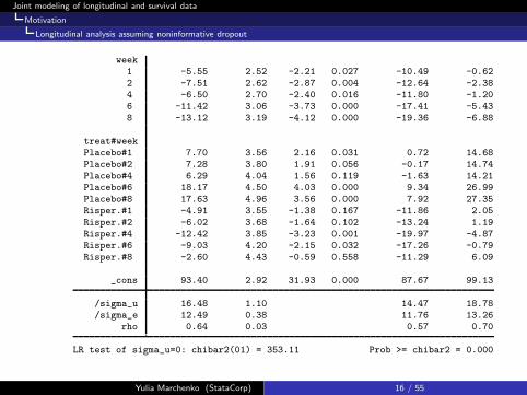
with m subjects (i = 1, 2, . . . ,m) and ni observations persubject (j = 1, 2, . . . , ni ), where βLxij represents a saturatedmodel with one coefficient for each treat and week

combination.

U ′i s ∼ i.i.d. N(0, σ2

u) are random intercepts which inducedependence within subjects.

ǫ′ijs ∼ i.i.d. N(0, σ2e ) are error terms.



Motivation


We use xtreg, mle to fit a simple random-intercept modelby using maximum likelihood (ML) with fixed effects for eachcombination of treatment and time:

. xtset idpanel variable: id (balanced)

. xtreg panss i.treat##i.week, mle nolog

Random-effects ML regression Number of obs = 685

Group variable: id Number of groups = 150

Random effects u_i ~ Gaussian Obs per group:min = 1

avg = 4.6max = 6

LR chi2(17) = 105.58Log likelihood = -2861.58 Prob > chi2 = 0.0000

panss Coef. Std. Err. z P>|z| [95% Conf. Interval]

treatPlacebo -2.00 4.14 -0.48 0.629 -10.11 6.11Risper. -2.14 4.14 -0.52 0.605 -10.25 5.97



Motivation


week1 -5.55 2.52 -2.21 0.027 -10.49 -0.62

2 -7.51 2.62 -2.87 0.004 -12.64 -2.384 -6.50 2.70 -2.40 0.016 -11.80 -1.206 -11.42 3.06 -3.73 0.000 -17.41 -5.43

8 -13.12 3.19 -4.12 0.000 -19.36 -6.88

treat#weekPlacebo#1 7.70 3.56 2.16 0.031 0.72 14.68

Placebo#2 7.28 3.80 1.91 0.056 -0.17 14.74Placebo#4 6.29 4.04 1.56 0.119 -1.63 14.21Placebo#6 18.17 4.50 4.03 0.000 9.34 26.99

Placebo#8 17.63 4.96 3.56 0.000 7.92 27.35Risper.#1 -4.91 3.55 -1.38 0.167 -11.86 2.05

Risper.#2 -6.02 3.68 -1.64 0.102 -13.24 1.19Risper.#4 -12.42 3.85 -3.23 0.001 -19.97 -4.87Risper.#6 -9.03 4.20 -2.15 0.032 -17.26 -0.79

Risper.#8 -2.60 4.43 -0.59 0.558 -11.29 6.09

_cons 93.40 2.92 31.93 0.000 87.67 99.13

/sigma_u 16.48 1.10 14.47 18.78/sigma_e 12.49 0.38 11.76 13.26

rho 0.64 0.03 0.57 0.70

LR test of sigma_u=0: chibar2(01) = 353.11 Prob >= chibar2 = 0.000



Motivation

Mean PANSS profiles over time

All three groups demonstrate a decrease in mean PANSSscore over time, at least in the first three weeks.

. quietly margins i.week, over(treat) predict(xb)

. marginsplot

Variables that uniquely identify margins: week treat60

7080

9010

011

0Li

near

Pre

dict

ion

0 1 2 4 6 8Time (weeks)

Haloperidol PlaceboRisperidone

Predictive Margins of week with 95% CIs



Motivation

Is assumption of random dropout plausible?

Given that many subjects dropped out of the study because ofinadequate response, the observed decrease in PANSS scoresmay be due to the dropout of subjects with high PANSSscores.

We can look at the observed mean profiles over time for eachmissing-value pattern, similarly to Figure 13.4 in Diggle et al.(2002).

. keep if nobs>1

(12 observations deleted)

. by week nobs, sort: egen panss_ptrn = mean(panss)(205 missing values generated)

. qui reshape wide panss_ptrn, i(id week) j(nobs)

. twoway line panss_ptrn* week, sort legend(order(5 "Completers")) ///

> title(Observed mean PANSS by dropout pattern) ytitle(PANSS)



Motivation

Is assumption of random dropout plausible?

7080

9010

011

0P

AN

SS

0 2 4 6 8Time (weeks)

Completers

Observed mean PANSS by dropout pattern

There is a steep increase in the mean PANSS scoreimmediately prior to dropout for all dropout patterns exceptcompleters.This provides strong empirical evidence that dropout is relatedto PANSS scores and is thus informative (nonrandom).



Motivation

Dropout process

We may also be interested in a dropout process itself. Forexample, is there a difference between dropout rates becauseof “inadequate response” among groups?

We can use standard methods of survival analysis to answerthis question.

We can treat dropout time as our analysis time and whetherthe dropout is because of inadequate response as our event ofinterest or failure.



Motivation

Dropout process

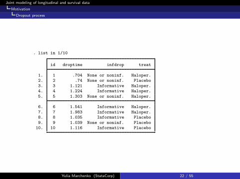
Data description:

. use panss_surv

(Dropout times for study of drug treatments for schizophrenia)

. describe

Contains data from panss_surv.dtaobs: 150 Dropout times for study of drug

treatments for schizophreniavars: 4 29 Aug 2016 12:07size: 1,200 (_dta has notes)

storage display value

variable name type format label variable label

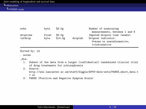
id int %8.0g Patient identifierdroptime float %8.0g Imputed dropout time (weeks)infdrop byte %14.0g droplab Dropout indicator:

0=none or noninfiormative;1=informative

treat byte %11.0g treatlab Treatment identifier:1=Haloperidol, 2=Placebo,

3=Risperidone

Sorted by: id



Motivation

Dropout process

. list in 1/10

id droptime infdrop treat

1. 1 .704 None or noninf. Haloper.2. 2 .74 None or noninf. Placebo

3. 3 1.121 Informative Haloper.4. 4 1.224 Informative Haloper.

5. 5 1.303 None or noninf. Haloper.

6. 6 1.541 Informative Haloper.

7. 7 1.983 Informative Haloper.8. 8 1.035 Informative Placebo

9. 9 1.039 None or noninf. Placebo10. 10 1.116 Informative Placebo



Motivation

Cox proportional hazards model

Cox proportional hazards model:

hi (t|treat)=h0(t) exp(βS1 1.treati+βS

2 2.treati+βS3 3.treati )

(2)

where t is the dropout time droptime and i = 1, 2, . . . ,m.

Baseline hazard h0(t) is left unspecified.

A constant term βS0 is absorbed into the baseline hazard.

Coefficients βS1 , β

S2 , and βS

3 model subject-specific hazards asa function of the treatment group. In general, covariates mayalso depend on time t.

Subject-specific hazards are proportional.

Exponentiated coefficients are hazard ratios.



Motivation


Declare survival-time data:

. stset droptime, failure(infdrop)

failure event: infdrop != 0 & infdrop < .

obs. time interval: (0, droptime]exit on or before: failure

150 total observations0 exclusions

150 observations remaining, representing63 failures in single-record/single-failure data

863.624 total analysis time at risk and under observationat risk from t = 0

earliest observed entry t = 0

last observed exit t = 8.002



Motivation


Fit Cox model:

. stcox i.treat

failure _d: infdrop

analysis time _t: droptime

Iteration 0: log likelihood = -293.97982Iteration 1: log likelihood = -288.97387

Iteration 2: log likelihood = -288.86504Iteration 3: log likelihood = -288.86498

Refining estimates:Iteration 0: log likelihood = -288.86498

Cox regression -- Breslow method for ties

No. of subjects = 150 Number of obs = 150No. of failures = 63

Time at risk = 863.6239911LR chi2(2) = 10.23

Log likelihood = -288.86498 Prob > chi2 = 0.0060

_t Haz. Ratio Std. Err. z P>|z| [95% Conf. Interval]

treatPlacebo 1.81 0.53 2.04 0.041 1.02 3.21

Risper. 0.68 0.24 -1.12 0.262 0.34 1.34



Motivation


Redisplay results as coefficient estimates (for latercomparison):

. stcox, nohr

Cox regression -- Breslow method for ties

No. of subjects = 150 Number of obs = 150

No. of failures = 63Time at risk = 863.6239911

LR chi2(2) = 10.23Log likelihood = -288.86498 Prob > chi2 = 0.0060

_t Coef. Std. Err. z P>|z| [95% Conf. Interval]

treat

Haloper. 0.00 (empty)Placebo 0.59 0.29 2.04 0.041 0.02 1.16

Risper. -0.39 0.35 -1.12 0.262 -1.07 0.29



Motivation

Survivor functions by treatment groups

Plot survivor functions in three treatment groups:

. stcurve, survival at1(treat=1) at2(treat=2) at3(treat=3)

.4.6

.81

Sur

viva

l

0 2 4 6 8Time to dropout (weeks)

Haloperidol (treat=1) Placebo (treat=2)Risperidone (treat=3)

Cox proportional hazards regression

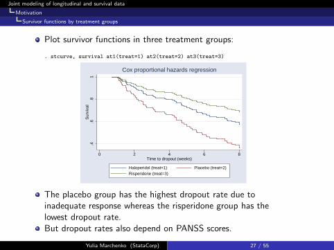
The placebo group has the highest dropout rate due toinadequate response whereas the risperidone group has thelowest dropout rate.But dropout rates also depend on PANSS scores.



Joint analysis

Revisiting PANSS study

Whether we are interested:

In the longitudinal analysis of PANSS trajectory over time indifferent groups,In the survival analysis comparing dropout rates among thegroups, orIn both types of analysis,

we cannot perform them separately, given that the twooutcomes may be correlated.

We should consider joint analysis of these data.



Joint analysis

Goals

Joint analysis should be able to incorporate the specificfeatures of longitudinal and survival data.

Joint analysis should be equivalent to the correspondingseparate analysis in the absence of an association between thelongitudinal and survival outcomes.

Tsiatis et al. (1995), Wulfsohn and Tsiatis (1997), andHenderson et al. (2000) considered a joint model that linksthe longitudinal and survival outcomes through a sharedlatent process.



Joint analysis

PANSS analysis accounting for informative dropout

Let’s fit a model that accounts for informative dropout.

Consider the following joint random-intercept Cox modelbased on separate models (1) and (2):

panssij =βLxij + Ui + ǫij

hi(t)=h0(t) exp(βSi.treati + γUi) (3)

Random intercepts U ′i s are now shared between the two

models and induce dependence between the longitudinaloutcome panss and survival outcome droptime.

More generally, I will refer to model (3) as a jointrandom-intercept Cox model, in which survival outcome ismodeled semiparametrically using the Cox model.




You can use forthcoming, user-written suite jm to performjoint analysis of longitudinal and survival data.

Command jmxtstset declares your longitudinal and survivaldata.

Command jmxtstcox fits joint random-intercept Cox models,similar to model (3).

Command jmxtstcurve plots survivor, hazard, andcumulative hazard functions after jmxtstcox.

Other Stata postestimation features such as predict, test,nlcom, margins, etc. are also available.




Data declaration—jmxtstset

To fit joint models using jmxtstcox, you must first declareyour longitudinal and survival data using jmxtstset.

Longitudinal and survival data are typically saved in differentfiles. To perform estimation, all data should be in one filewith longitudinal data saved in a long format (with multipleobservations per subject saved in rows).

jmxtstset provides a syntax that combines the two datasetsand performs declaration, and provides a syntax that declaresan already combined dataset.




Data declaration—jmxtstset

jmxtstset combines the syntaxes of stset and xtset.Syntax for the combined dataset:

. jmxtstset idvar timevar, xt(is xt)|st(is st) failure(failvar)[

stsetopts]

is xt and is st are binary variables identifying longitudinal andsurvival observations, respectively; only one of them must bespecified in the respective option.

Syntax for separate datasets with survival dataset in memory:

. use survfile

. jmxtstset idvar timevar using longfile, st failure(failvar)[

stsetopts]

Syntax for separate datasets with longitudinal dataset inmemory:

. use longfile

. jmxtstset idvar timevar using survfile, xt failure(failvar)[

stsetopts]




Estimation

Command jmxtstcox performs estimation.

It fits a random-intercept Cox model to the survival andlongitudinal outcomes.

jmxtstcox uses nonparametric ML to estimate modelparameters. The estimation method is anexpectation-maximization algorithm. The standard errors areobtained using the observed information matrix (Louis 1982).




Comparison with other Stata commands for joint analysis

Command gsem (help gsem) can be used to fit joint modelswith flexible specification of latent processes, but in whichsurvival outcome is modeled parametrically.

User-written command stjm (Crowther et al. 2013) can beused to fit joint random-intercept and random-coefficientmodels. The survival outcome is again modeledparametrically, but flexible parametric survival models(Royston and Lambert 2011) are also supported.

User-written command jmxtstcox currently supports onlyjoint random-intercept models, but it allows to model thesurvival outcome semiparametrically, without any parametricassumptions for the baseline hazard.




Data declaration

Let’s now analyze PANSS scores and dropout times jointly byfiting the random-intercept Cox model (3).

The longitudinal data are saved in panss long.dta and thesurvival data are saved in panss surv.dta.

We first use jmxtstset to combine survival and longitudinaldatasets and to declare the combined data:

. use panss_surv

(Dropout times for study of drug treatments for schizophrenia)

. jmxtstset id droptime using panss_long, st failure(infdrop)

-----------------------------------LONGITUDINAL-------------------------------

id: idfilename: panss_long.dta

900 total observations

0 exclusions

900 observations remaining150 subjects




Data declaration

-------------------------------------SURVIVAL---------------------------------

id: id

failure event: infdrop != 0 & infdrop < .obs. time interval: (droptime[_n-1], droptime]

exit on or before: failure

150 total observations

0 exclusions

150 observations remaining, representing

150 subjects63 failures in single-failure-per-subject data

863.624 total analysis time at risk and under observationat risk from t = 0

earliest observed entry t = 0

last observed exit t = 8.002




Estimation

We now use jmxtstcox to fit the joint model:

. jmxtstcox (_xt: panss i.treat##i.week) (_st: i.treat), nolog

longitudinal depvar: panss

failure _d: infdropanalysis time _t: droptime

Joint model of longitudinal and survival dataBreslow method for ties

Subject id: id Total subjects = 150

Longitudinal (_xt): Survival (_st):

No. of subjects = 150 No. of subjects = 150No. of obs = 685 No. of obs = 150

No. of failures = 63

Time at risk = 863.62

Wald chi2(19) = 112.90Observed log likelihood = -3194.739326 Prob > chi2 = 0.0000




Estimation

Coef. Std. Err. z P>|z| [95% Conf. Interval]

pansstreat

Placebo -2.00 4.16 -0.48 0.631 -10.16 6.16

Risper. -2.14 4.16 -0.51 0.607 -10.30 6.02

week1 -5.55 2.51 -2.21 0.027 -10.48 -0.63

2 -7.24 2.61 -2.77 0.006 -12.36 -2.134 -6.12 2.70 -2.27 0.023 -11.40 -0.836 -10.61 3.05 -3.48 0.001 -16.59 -4.63

8 -12.20 3.18 -3.84 0.000 -18.43 -5.97

treat#weekPlacebo#1 7.69 3.55 2.17 0.030 0.73 14.66Placebo#2 7.65 3.79 2.02 0.044 0.22 15.09

Placebo#4 7.03 4.03 1.75 0.081 -0.86 14.93Placebo#6 18.74 4.49 4.18 0.000 9.95 27.54

Placebo#8 18.43 4.94 3.73 0.000 8.75 28.11Risper.#1 -4.91 3.54 -1.39 0.166 -11.84 2.03

Risper.#2 -6.08 3.67 -1.65 0.098 -13.28 1.13Risper.#4 -12.30 3.84 -3.20 0.001 -19.83 -4.77Risper.#6 -9.12 4.19 -2.18 0.029 -17.33 -0.91

Risper.#8 -2.82 4.42 -0.64 0.524 -11.48 5.85

_cons 93.40 2.93 31.85 0.000 87.65 99.15




Estimation

_ttreat

Placebo 0.77 0.34 2.23 0.026 0.09 1.44Risper. -0.49 0.39 -1.26 0.207 -1.26 0.27

/gamma 0.05 0.01 0.04 0.07

/sigma2_u 281.22 37.30 208.11 354.34

/sigma2_e 155.29 9.47 136.73 173.85

LR test of gamma = 0: chi2(1) = 37.41 Prob >= chi2 = 0.0000

The association parameter γ has an estimate of 0.05 with a95% CI of (0.04, 0.07), which implies a positive associationbetween PANSS scores and dropout times—the higher thePANSS score, the higher the chance of dropout.

The LR test of no latent association (H0: γ = 0) withχ21 = 37.41 provides strong evidence against a random-dropout

model.



Comparison of results with analysis ignoring dropout

Longitudinal outcome

The estimated random-intercept variance is slightly largerunder the joint, informative dropout model.

Variable inform noninf

sigma2_u

_cons 281.22 271.7537.30 36.19

0.00 0.00

sigma2_e

_cons 155.29 155.959.47 9.55

0.00 0.00

legend: b/se/p




Mean PANSS profiles over time for each group

As with xtreg, we can compute and plot estimated meanPANSS profiles after jmxtstcox.

. qui margins i.week, over(treat) predict(xb xt)

. marginsplot

Variables that uniquely identify margins: week treat60

7080

9010

011

0Li

near

Pre

dict

ion

For

Lon

gitu

dina

l Sub

mod

el

0 1 2 4 6 8Time (weeks)


Predictive Margins of week with 95% CIs




Mean PANSS profiles over time for each group

We can overlay the estimated mean profiles with the observedmean profiles.

6070

8090

100

110

PA

NS

S

0 1 2 4 6 8Time (weeks)

Haloperidol PlaceboRisperidone Observed means

Estimated means from joint model with 95% CIs

The estimated mean profiles from the joint model are higherthan the observed mean profiles because the former represent“dropout-free” profiles—subjects with high PANSS scorestend to drop out, which leads to lower observed mean values.




Survival outcome

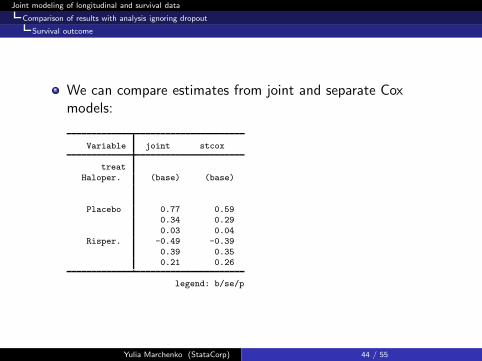
We can compare estimates from joint and separate Coxmodels:

Variable joint stcox

treat

Haloper. (base) (base)

Placebo 0.77 0.590.34 0.29

0.03 0.04Risper. -0.49 -0.39

0.39 0.350.21 0.26

legend: b/se/p




Survivor functions of times to dropout

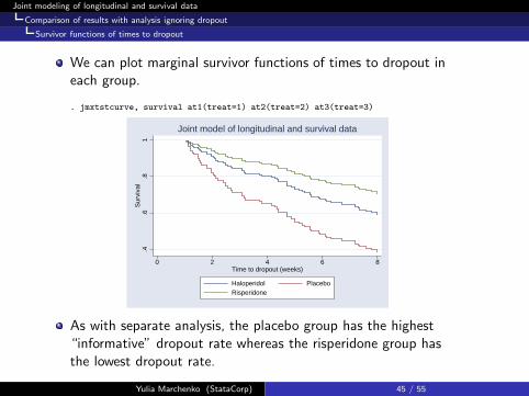
We can plot marginal survivor functions of times to dropout ineach group.

. jmxtstcurve, survival at1(treat=1) at2(treat=2) at3(treat=3)

.4.6

.81

Sur

viva

l



Joint model of longitudinal and survival data

As with separate analysis, the placebo group has the highest“informative” dropout rate whereas the risperidone group hasthe lowest dropout rate.




Survivor functions of times to dropout

In fact, survival estimates from joint and separate analyses aresimilar:

.4.6

.81

Sur

viva

l


Haloperidol PlaceboRisperidone Separate analyses

Joint analysis versus separate analysis




Random-intercept model (3) can be extended to allow formore flexible latent associations motivated by practice; seeHenderson (2000) for details.For example, a joint random-coefficient Cox modeladditionally includes a random slope on time in thelongitudinal model and an association through the randomslope in the survival model.

panssij = βLxij + U1i + week× U2i + ǫij

hi (t) = h0(t) exp(βSi.treati + γ1U1i + γ2U2i ) (4)

A joint random-trajectory Cox model extends therandom-coefficient model (4) to include an entire stochasticlongitudinal trajectory.

panssij = βLxij + U1i + week× U2i + ǫij

hi(t) = h0(t) exp(βSi.treati + γ1U1i + γ2U2i + γ3Wi(t))

Wi(t) = U1i + t × U2i (5)




Semiparametric Cox submodels in (3), (4), and (5) can bereplaced with a parametric survival model, if appropriate.

For example, with an exponential model:

hi (t) = t exp(βSi.treati + γUi) (3a)

Or, with a Weibull model:

hi(t) = ptp−1 exp(βSi.treati + γUi) (3b)

Such parametric models can be fit using, for example, gsem,but software for the corresponding semiparametric models isnot available yet.




For example, a joint random-intercept model using gsem:

. gsem (panss <- i.treat##i.week U[id]@1)> (droptime <- i.treat U[id]@gamma, family(weibull, failure(infdrop)))

A joint random-coefficient model:

. gsem (panss <- i.treat##i.week U1[id]@1 c.week#U2[id]@1)> (droptime <- i.treat U1[id]@gamma1 U2[id]@gamma2,> family(weibull, failure(infdrop))),> covstructure(U1[id] U2[id], unstructured)



Summary

Summary

Joint analysis of longitudinal and survival outcomes isnecessary to obtain unbiased inference when the twooutcomes are correlated.Joint analysis can be used, for example, 1) to evaluate effectsof baseline covariates on longitudinal and survival outcomes,2) to evaluate effects of time-dependent covariates on survivaloutcome; and 3) to account for informative dropout inlongitudinal analysis.You can use user-written command jmxtstcox to fit a jointrandom-intercept Cox model.You can use gsem to fit joint models that can accommodatemore flexible specifications of a latent process andnoncontinuous longitudinal outcomes. The survival outcome,however, is modeled parametrically.Also see user-written command stjm for fitting flexibleparametric joint models of longitudinal and survival data.



Future work

Future work

Support of semiparametric Cox models with more flexiblelatent associations such as a random-coefficient model (4)and a random-trajectory model (5).

Support of noncontinuous longitudinal outcomes includingbinary and count outcomes.

Support of nonproportional hazards via transformationsurvival models (Zeng and Lin 2007).

More postestiomation features such as dynamic predictionsand model diagnostics for joint analysis of longitudinal andsurvival data.



Acknowledgement

Acknowledgement

Work on the jm suite was supported by the NIH Phase II SBIR(HHSN261201200096C) contract titled “Software for ModernExtensions of the Cox model” to StataCorp LP with consultantsDanyu Lin, Department of Biostatistics, University of NorthCarolina at Chapel Hill and Donglin Zeng, Department ofBiostatistics, University of North Carolina at Chapel Hill.



References

References

Crowther, M. J., Abrams, K. R., and P. C. Lambert. 2013. Jointmodeling of longitudinal and survival data. Stata Journal 13:165–184.

Diggle, P. J. 1998. Dealing with missing values in longitudinalstudies. In Everitt, B. S., and G. Dunn. (eds.) Recent Advances in

the Statistical Analysis of Medical Data. London: Arnold, pp.203–228.

Diggle, P. J., P. Heagerty, K. Y. Liang, and S. L. Zeger. 2002.Analysis of Longitudinal Data. 2nd Ed. Oxford University Press.



References

References (cont.)

Henderson, R., P. Diggle, and A. Dobson. 2000. Joint modeling oflongitudinal measurements and event time data. Biostatistics 4:465–480.

Louis, T. A. 1982. Finding the observed information matrix whenusing the EM algorithm. Journal of the Royal Statistical Society B.

44: 226–233.

Royston, P., and P. C. Lambert. 2011. Flexible Parametric

Survival Analysis Using Stata: Beyond the Cox Model. CollegeStation, TX: Stata Press.



References

References (cont.)

Tsiatis, A. A., V. DeGruttola, and M. S. Wulfsohn. 1995.Modeling the relationship of survival to longitudinal data measuredwith error: Applications to survival and CD4 counts in patientswith AIDS. Journal of the American Statistical Association 90:27–37.

Wulfsohn, M. S. and A. A. Tsiatis. 1997. A joint model forsurvival and longitudinal data measured with error. Biometrics 53:330–339.

Zeng, D. and D. Y. Lin. 2007. Maximum likelihood estimation insemiparametric regression models with censored data (withdiscussion). Journal of the Royal Statistical Society B, 69,507–564.


Date post:	26-Jan-2019
Category:	Documents
Upload:	phamdang
View:	256 times
Download:	1 times

Joint modeling of longitudinal and survival data · Joint modeling of longitudinal and survival...

Documents