Page 1
THE COOPER UNION FOR THE ADVANCEMENT OF SCIENCE AND ART
ALBERT NERKEN SCHOOL OF ENGINEERING
Joint Spatial-Temporal Equalization
of 3G HF Communicationsby
Samantha G. Massengill
A thesis submitted in partial fulfillment
of the requirements for the degree of
Master of Engineering
September 3, 2013
Advisor
Dr. Sam M. Keene
Page 2
THE COOPER UNION FOR THE ADVANCEMENT OF SCIENCE AND ART
ALBERT NERKEN SCHOOL OF ENGINEERING
This thesis was prepared under the direction of the Candidate’s Thesis Advisor and
has received approval. It was submitted to the Dean of the School of Engineering and
the full Faculty, and was approved as partial fulfillment of the requirements for the
degree of Master of Engineering.
Dr. Teresa A. Dahlberg
Dean, School of Engineering
Dr. Sam M. Keene
Candidate’s Thesis Advisor
Page 3
Acknowledgments
Thank you to Sam Keene for his patience and guidance; to Glen Mabey for his
mentorship, encouragement, and friendship; to Ryan Casey and Jason Polendo for
their willingness to share time and expertise; to my parents for their love, support,
and understanding; to my friends for showing me what it means to truly be part
of a community; to Bryan for joyfully, lovingly, and tirelessly supporting me and
encouraging me in every way he knows how; and to God for sustaining me and giving
me strength.
i
Page 4
Abstract
The high frequency (HF) spectrum is home to many military communication sig-
nals that rely on receivers to accurately equalize, demodulate, and decode signals of
interest. This is not a trivial task when faced with the challenges that arise from sig-
nals being reflected back to Earth by the ionosphere. To combat HF channel e↵ects,
it is desirable to exploit spatial diversity; however, the design of diversity receivers
becomes complicated especially when limited channel information is available.
This work describes the design and testing of an HF military standard (MIL-STD)
188-141B (ALE3G) diversity receiver that uses a joint spatial-temporal equalizer to
perform the dual task of combining and equalizing the signals received by multiple
antennas prior to demodulation and decoding of transmitted data. The receiver re-
quires no prior knowledge of the channel, array geometry, or angle of arrival of the
multipath signal. This design is evaluated against two diversity receivers that perform
linear combining followed by single-channel equalization. For various adaptive filter
parameters, the joint spatial-temporal equalizer has a shorter convergence time and
lower mean squared error (MSE) than the combiner and equalizer. At low SNRs, the
spatial-temporal equalizer also outperforms in terms of bit error rate (BER), showing
up to a 10 dB improvement over the single-channel equalizer structure.
ii
Page 5
Contents
1 Introduction 11.1 Motivation . . . . . . . . . . . . . . . . . . . . . . . . . . . . . . . . . 11.2 Problem Statement . . . . . . . . . . . . . . . . . . . . . . . . . . . . . 21.3 Previous Work . . . . . . . . . . . . . . . . . . . . . . . . . . . . . . . 21.4 Proposed Solution . . . . . . . . . . . . . . . . . . . . . . . . . . . . . 5
2 HF Communications 72.1 Introduction to HF . . . . . . . . . . . . . . . . . . . . . . . . . . . . . 72.2 The Ionosphere . . . . . . . . . . . . . . . . . . . . . . . . . . . . . . . 72.3 Watterson Model . . . . . . . . . . . . . . . . . . . . . . . . . . . . . . 92.4 MIL-STD-188-141B . . . . . . . . . . . . . . . . . . . . . . . . . . . . 10
3 Adaptive Equalization 163.1 Basics of Equalization . . . . . . . . . . . . . . . . . . . . . . . . . . . 163.2 LMS Filtering . . . . . . . . . . . . . . . . . . . . . . . . . . . . . . . . 193.3 RLS Filtering . . . . . . . . . . . . . . . . . . . . . . . . . . . . . . . . 20
4 Receiver Diversity 234.1 Basics of Diversity . . . . . . . . . . . . . . . . . . . . . . . . . . . . . 234.2 Combining Techniques . . . . . . . . . . . . . . . . . . . . . . . . . . . 24
5 Joint Spatial-Temporal Equalization 265.1 System Model . . . . . . . . . . . . . . . . . . . . . . . . . . . . . . . . 265.2 Simulation Details . . . . . . . . . . . . . . . . . . . . . . . . . . . . . 30
6 Experimental Results 326.1 Introduction . . . . . . . . . . . . . . . . . . . . . . . . . . . . . . . . . 326.2 Equalizer Convergence . . . . . . . . . . . . . . . . . . . . . . . . . . . 326.3 Receiver Performance . . . . . . . . . . . . . . . . . . . . . . . . . . . 44
7 Conclusions and Future Work 49
iii
Page 6
A MATLAB Code 51A.1 ALE3G Signal Generator . . . . . . . . . . . . . . . . . . . . . . . . . 51A.2 ALE3G Demodulator . . . . . . . . . . . . . . . . . . . . . . . . . . . . 56A.3 Spatial-Temporal Equalizer . . . . . . . . . . . . . . . . . . . . . . . . 61A.4 Watterson Channel Simulator . . . . . . . . . . . . . . . . . . . . . . . 63A.5 ALE3G Equalizer Comparison . . . . . . . . . . . . . . . . . . . . . . 68
Bibliography 73
Page 7
List of Figures
2.1 Ionospheric refraction [3] . . . . . . . . . . . . . . . . . . . . . . . . . . 8
2.2 Burst waveform characteristics [13] . . . . . . . . . . . . . . . . . . . . 12
2.3 BW5 descrambling, SNR 30 dB . . . . . . . . . . . . . . . . . . . . . . 13
2.4 BW5 structure [13] . . . . . . . . . . . . . . . . . . . . . . . . . . . . . 14
2.5 Walsh modulation of coded bits to tribit sequences [18] . . . . . . . . . 14
2.6 BW5 convolutional encoder [21] . . . . . . . . . . . . . . . . . . . . . . 15
3.1 Symbol-spaced linear equalizer [16] . . . . . . . . . . . . . . . . . . . . 18
4.1 Linear combiner [6] . . . . . . . . . . . . . . . . . . . . . . . . . . . . . 24
5.1 Linear combiner followed by single-channel equalizer . . . . . . . . . . 27
5.2 Joint spatial-temporal equalizer . . . . . . . . . . . . . . . . . . . . . . 28
6.1 Equalized symbols: 24 taps, RLS(0.99), SNR 20 dB, 4 diversity branches 36
6.2 Learning curves: 24 taps, RLS(0.99), SNR 20 dB, 4 diversity branches 36
6.3 Equalized symbols: 24 taps, RLS(0.95), SNR 20 dB, 4 diversity branches 37
6.4 Learning curves: 24 taps, RLS(0.95), SNR 20 dB, 4 diversity branches 37
6.5 Equalized symbols: 12 taps, RLS(0.95), SNR 10 dB, 4 diversity branches 38
6.6 Learning curves: 12 taps, RLS(0.95), SNR 10 dB, 4 diversity branches 38
v
Page 8
6.7 Equalized symbols: 12 taps, RLS(0.90), SNR 20 dB, 4 diversity branches 39
6.8 Learning curves: 12 taps, RLS(0.90), SNR 20 dB, 4 diversity branches 39
6.9 Equalized symbols: 36 taps, LMS(0.05), SNR 10 dB, 4 diversity branches 40
6.10 Learning curves: 36 taps, LMS(0.05), SNR 10 dB, 4 diversity branches 40
6.11 Equalized symbols: 36 taps, LMS(0.10), SNR 20 dB, 4 diversity branches 41
6.12 Learning curves: 36 taps, LMS(0.10), SNR 20 dB, 4 diversity branches 41
6.13 Equalized symbols: 12 taps, LMS(0.15), SNR 20 dB, 4 diversity branches 42
6.14 Learning curves: 12 taps, LMS(0.15), SNR 20 dB, 4 diversity branches 42
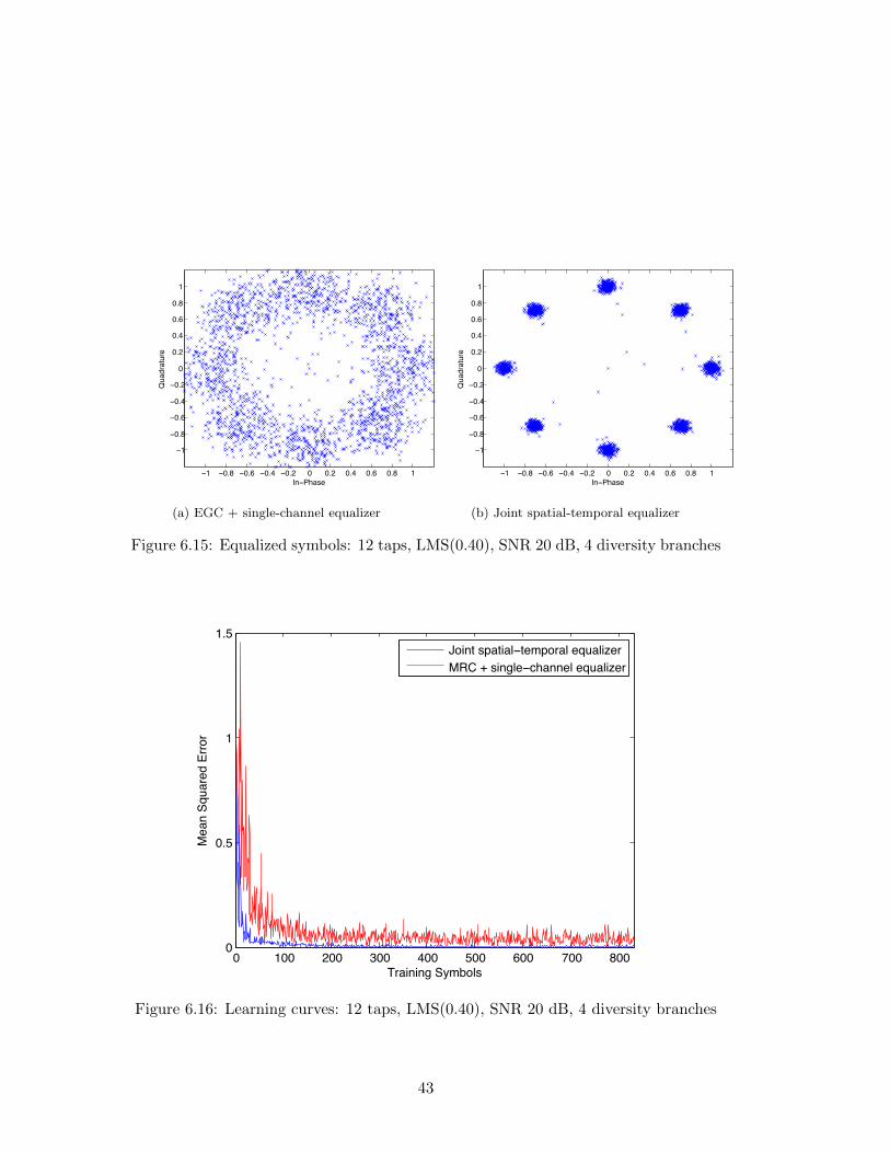
6.15 Equalized symbols: 12 taps, LMS(0.40), SNR 20 dB, 4 diversity branches 43
6.16 Learning curves: 12 taps, LMS(0.40), SNR 20 dB, 4 diversity branches 43
6.17 BER versus SNR for two receivers: 12 taps, RLS(0.99) . . . . . . . . . 45
6.18 BER versus SNR for two receivers: 12 taps, RLS(0.95) . . . . . . . . . 46
6.19 BER versus SNR for two receivers: 12 taps, RLS(0.90) . . . . . . . . . 47
6.20 BER versus SNR for two receivers: 24 taps, LMS(0.01) . . . . . . . . . 48
Page 9
List of Tables
2.1 ITU-R F.1487 Ionospheric Channel Parameters [20] . . . . . . . . . . . 10
6.1 Equalizer convergence comparisons, LMS . . . . . . . . . . . . . . . . 34
6.2 Equalizer convergence comparisons, RLS . . . . . . . . . . . . . . . . . 35
vii
Page 10
Chapter 1
Introduction
1.1 Motivation
Over the past decade, high frequency (HF) radio communications have witnessed a
period of renewal, largely due to the advances of third-generation (3G) and wideband
HF (WBHF) technologies [13]. Due to increasing popularity amongst military and
governmental communities, this thesis focuses on improving the reception of 3G au-
tomatic link establishment (ALE3G) tranmissions. Oftentimes, reception of ALE3G
signals is done by a third party for whom the transmitted message was not originally
intended. In addition to HF radio receivers having to overcome ionospheric channel
e↵ects, there are additional challenges that the passive listener faces which do not exist
for cooperative receivers; for example, the receiver may require additional information
from the transmitter in order to perform timing synchronization, demodulation, or
decoding. Furthermore, the channel quality is potentially worse for a passive listener
since he may be hundreds of kilometers away from the cooperative receiver. This
thesis addresses the need for improved receivers in the presence of HF channel e↵ects,
particularly when minimal information is available to the receiver.
1
Page 11
1.2 Problem Statement
There are multiple ways in which a signal propagating through an HF channel can
be distorted. If copies of the signal are delayed in time and this delay is on the order
of one symbol period, intersymbol interference (ISI) can occur as a result. In a digital
communications system, equalizers are used to mitigate ISI by creating a filter that
estimates the inverse of the channel and then passing the ISI-corrupted signal through
the filter to recover the original transmitted message.
In addition to equalization, the reliability of receiving a multipath signal can im-
prove greatly with the use of receiver diversity. For a time-varying channel with
fading, using more than one receive antenna is useful since it is unlikely that each
antenna will be experiencing the same fading. The goal of this work is to introduce a
spatial-temporal equalizer that jointly performs equalization and diversity combining
in an HF channel. Possible benefits of introducing this scheme include the receiver
requiring less channel state information, lower computational complexity, better per-
formance under certain conditions, and reducing the need for additional components
in a modular software-defined radio dataflow architecture.
1.3 Previous Work
There has been a substantial amount of research done in investigating combined
spatial-temporal equalization for digital communications systems. In [15], subopti-
mal solutions to spatial-temporal decision feedback equalization were investigated in
hopes of greatly reducing computational complexity while still preserving good per-
formance. The authors compare three algorithms: the general beam decision feed-
back equalizer (GB-DFE), the multiple independent beam decision feedback equalizer
2
Page 12
(MIB-DFE), and simultaneous beamforming and equalization iterating with the LS-
algorithm (SBE-LS). The GB-DFE is simply a MISO FIR decision feedback equalizer
where the signals from each array are delayed and summed before equalization. The
MIB-DFE, proposed by the authors, performs optimization on antenna weights prior
to equalization where the combiner weights and equalizer weights are optimized us-
ing two di↵erent criteria. The last algorithm, SBE-LS, also proposed by the authors,
optimizes beamformer weights and equalizer coe�cients using two RLS filters. The
algorithm is first applied to the equalizer coe�cients while holding the beamformer
weights fixed, then applied to the beamformer weights while equalizer coe�cients are
fixed. It is shown that for short training sequences, the MIB-DFE outperforms the
other two algorithms and requires the least number of computations.
In [8], it is shown that a joint space-time DFE (ST-DFE) is superior to a structure
having a preselection diversity switch followed by a temporal DFE for frequency-
selective cellular fading channels. For the ST-DFE, the authors use a QR-decomposi-
tion type of RLS algorithm for the weight adaptation due to its e�cient and stable
implementation.
In [7], antenna combiner weights and equalizer weights are jointly optimized but
remain separate entities. Typically, the combiner chooses its weights prior to symbol
detection and does not have access to the newest information available. The authors
design an equalizer-assisted combiner, where the error from the equalizer is fed back
to help the combiner adjust its weights after symbol decisions have been made. The
combiner optimization is performed using the LMS algorithm. A second algorithm is
proposed that jointly minimizes the output cluster variance by using LMS to adapt
the equalizer weights and “filtered-X LMS” to adjust the combiner weights.
In [10], a spatial-temporal equalizer has been simulated using an adaptive tapped
3
Page 13
delay line antenna array and the Zero-Forcing algorithm and it was shown that this sys-
tem outperforms conventional temporal equalization. In [4], a multiple-input adaptive
combiner-equalizer is designed by adding tapped delay lines at each diversity branch
and then feeding the delayed signals to the inputs of a linear neuron whose weights are
updated using LMS or RLS. The authors show that replacing a maximal-ratio com-
biner and linear equalizer with a neural network yields results that are comparable in
performance but much less complex to implement especially on software defined ratio
(SDR) platforms.
Much work has also been done in simulating HF transmissions and proposing
enhancements to improve ALE3G reception. Simulations of MIL-STD-188-141B Ap-
pendix C, a US Department of Defense standard for HF radio where ALE3G is defined,
and STANAG 4538, a NATO standard that also defines ALE3G, are documented
in [25], [2], [14], [11], [12], [23] and proposed enhancements to STANAG 4538 are sug-
gested in [1]. Most of these simulations assume a single-channel receiver and minimal
research has been done in spatial diversity for HF communications. In [17], multi-
site combination is performed to improve demodulation of HF signals. The signals
are transmitted in Texas and received in Utah and Maryland, so receiving antennas
are separated too far apart to constitute spatial diversity. The author mentions joint
spatial-temporal equalization as a possibility for future work on HF demodulation.
In [5], blind spatial-temporal equalization in HF is developed using the Constant
Modulus Algorithm (CMA) on a polarization sensitive array of four collocated anten-
nas wherein spatial-temporal equalization improves performance significantly over the
single-channel case.
4
Page 14
1.4 Proposed Solution
The algorithm most similar to the one actually implemented in this thesis is pre-
sented in [22]. The authors use spatial diversity equalization to improve reliability
of underwater communications. Each channel is linearly equalized and the outputs
are combined using an adaptive multi-channel combiner driven by the RLS algorithm.
The combiner input signals from all diversity channels are concatenated together to
form a single composite input signal and similarly, a composite tap-weight vector is
what is updated during the RLS optimization.
This idea is extended for HF communications. Instead of equalizing each channel
prior to combining, these operations are done simultaneously such that the equalizer
weights and combiner weights are optimized jointly. The RLS filter composite input
vector and composite tap-weight vector are formed similarly as in [22] such that each
iteration of the RLS algorithm contains both temporal and spatial information. After
the algorithm is developed, it is tested against a more traditional receiver that first
combines and then equalizes.
The rest of the thesis is outlined as follows. Chapter 2 discusses an overview of
HF communications, the ionosphere and how to simulate its behavior using the Wat-
terson model, and MIL STD 188-141B (ALE3G), the standard implemented for use
in the simulations presented in this work. Chapter 3 gives an overview of equaliza-
tion, followed by summaries of the LMS and RLS adaptive filtering algorithms used
for adaptive equalization in this thesis. Next, Chapter 4 illustrates the basic princi-
ples and advantages of receiver diversity by first giving a brief overview of diversity
techniques and then focusing on spatial diversity and combining methods. Chapter 5
introduces the joint spatial-temporal equalizer developed in this work and describes
the simulation platform. Chapter 6 presents and discusses experimental results, and
5
Page 15
Chapter 7 draws conclusions and suggests possible avenues for future work.
6
Page 16
Chapter 2
HF Communications
2.1 Introduction to HF
High frequency (HF) radio waves are transmitted in the 3-30 MHz range and have
wavelengths of 200 m or less. Due to these relatively short wavelengths, HF radio was
originally overlooked for commercial use despite many desirable characteristics when
compared to longer wavelength radios. For example, global ranges can be attained
in the HF band with less power than longer wavelength radios and HF antennas
are easier to build. Satellite communications also achieve global ranges but require
additional infrastructure making them less cost e�cient than HF networks. Therefore,
it is common to see HF radio used as a backup for satellite communications [13].
2.2 The Ionosphere
HF radio is able to achieve global ranges due to waves refracting o↵ the ionosphere
as shown in Figure 2.1 where a man receives signals that traveled to him via two
di↵erent paths. This is an example of skywave propagation where signals are launched
7
Page 17
Figure 2.1: Ionospheric refraction [3]
skyward and are bounced back and forth between the Earth and the ionosphere. In
addition to skywaves, there exist surface waves and space waves in HF but neither
of these interact with the ionosphere. Surface wave propagation refers to signals
that travel near the Earth’s surface following its curvature such that over-the-horizon
ranges can be reached but not global ranges. Space waves are either line-of-sight
(direct) transmissions or signals that are reflected o↵ the Earth’s surface [3]. Skywaves
are more widely studied in HF channels due to the long distances these transmissions
can travel.
The ionosphere is a region of the atmosphere that has an abundance of free elec-
trons due to solar radiation and cosmic rays that ionize the air. The density of free
electrons and of gas molecules to be ionized varies with altitude. There are three
layers of the ionosphere: D layer, E layer, and F layer, in increasing distance from
the Earth. Due to the lowest level of ionizing radiation being the furthest from the
Sun, the D layer has a low electron density and high neutral gas density. The E layer
has higher electron density and lower neutral gas density, and the highest electron
8
Page 18
density and lowest neutral gas density are found in the F layer at approximately 300
km above the Earth’s surface. The F layer has an additional layer during the day due
to solar radiation, where the F1 layer is between the E layer and the F2 layer and the
F2 layer is simply referred to the F layer at night. When a wave interacts with the
ionosphere, the wave is refracted according to the ionosphere’s free electron density
and the wave’s frequency; a higher frequency will result in decreased refraction [13].
In addition to the unpredictable nature of the ionospheric channel as a result of
its dependence on solar activity, there exist losses in signal strength associated with
reflection and refraction. Additionally, fading in both time and frequency make the
HF channel even more cumbersome to deal with. Due to the dispersive nature of the
ionosphere, multiple copies of a single transmitted signal arrive at a receiver. The
di↵erent paths taken by the signal are each di↵erent lengths and therefore also have
di↵erent phases. This multipath propagation could cause intersymbol interference
due to spreading in time and multipath fading due to shifts in frequency. Other
potential causes of fading are the Faraday e↵ect and ray interference [13]. These
channel impairments create many challenges for engineers who make HF modems and
so there is a need for standardized channel models that are used for testing of such
modems.
2.3 Watterson Model
The widely accepted mathematical model used for HF testing is the Watterson
model [24]. The Watterson model assumes the signal travels as two paths, each
having equal losses and separated by a fixed di↵erential time delay. At the receiv-
ing antennas, additive white Gaussian noise (AWGN) is added to simulate thermal
noise. The model also assumes a Doppler spread which is a fading-gain process with
9
Page 19
Table 2.1: ITU-R F.1487 Ionospheric Channel Parameters [20]
Channel condition Delay spread (ms) Doppler spread (Hz)Low latitude, quiet 0.5 0.5Low latitude, moderate 2 1.5Low latitude, disturbed 6 10Mid-latitude, quiet 0.5 0.1Mid-latitude, moderate 1 0.5Mid-latitude, disturbed 2 1Mid-latitude, disturbed NVI 7 1High latitude, quiet 1 0.5High latitude, moderate 3 10High latitude, disturbed 7 30
a specified bandwidth. The ITU-R recommendation for Watterson channel simulator
representative values are shown in Table 2.1. Near vertical incidence (NVI) occurs
when a signal is sent almost straight up such that it is refracted back to a nearby
receiver that is separated from the transmitter by a physical obstruction. Engineers
who use the Watterson model to simulate HF channels must specify the delay spread,
Doppler spread, and SNR for their model.
2.4 MIL-STD-188-141B
Automatic link establishment (ALE) describes the process of finding and manag-
ing an HF frequency for voice and data (email, texting, file transfer, etc.) tra�c. To
combat increasing congestion in the HF band during the mid-1990’s and improve spec-
trum e�ciency, a third generation automatic link establishment (ALE3G) standard
was designed and described in the US Department of Defense MIL-STD-188-141B
Appendix C. ALE3G is also part of STANAG 4538, a NATO implementation that
includes additional capabilities not originally presented in MIL-STD-188-141B Ap-
pendix C. ALE3G is an 8-level PSK serial-tone waveform modulated onto an 1800 Hz
10
Page 20
carrier with a baud rate of 2400 symbols per second. Like most other HF communica-
tions signals, ALE3G is filtered to a 3-kHz bandwidth and uses single-sideband mode
of operation.
The physical layer of ALE3G is manifested as “burst waveforms”; to date, there
are six of these waveforms that have been defined in standards [21], [18]: BW0, BW1,
BW2, BW3, BW4, BW5, and a seventh, BW1+, which is a proprietary burst waveform
developed by Harris Corporation [1] and has been proposed as an enhancement to
the standard. Only two of these waveforms, BW2 and BW3, send data tra�c (of
varied duration), while the remaining BWs are used for shorter transmissions (fixed
duration) such as acknowledgements (ACKs), link establishment, link management,
network time synchronization, and channel probing.
Generally, the structure of each burst waveform has three sections of PN-spread
8-ary PSK symbols. The first section is the transmit level control (TLC), followed
by an acquisition preamble, and ending with a data section. The purpose of the
TLC section is to give the system enough time for its transmitter TLC and receiver
automatic gain control (AGC) to adjust and stabilize. The preamble section contains
a di↵erent sequence of symbols that are unique to each di↵erent burst waveform in
terms of the order of symbols, the duration of the preamble, or both the order and
duration. Each burst waveform also has a di↵erent payload duration and structure.
In general, burst waveforms undergo error correction coding, interleaving, symbol
formation, and PN spreading before they are modulated and transmitted. Unlike the
rest of the waveforms, BW2 does not use Walsh symbol formation and instead forms
symbols using a series of rotation, gray coding, and frame formation. See Figure 2.2
for a summary of burst waveform characteristics, excluding the proprietary BW1+.
To introduce redundancy, the payload bits for the burst waveforms that carry
11
Page 21
Figure 2.2: Burst waveform characteristics [13]
data information (BW2 and BW3) are encoding using convolutional encoding with
flush bits that are known to the receiver. For short burst waveforms (all but BW2
and BW3), the bits are encoded using tail-biting convolutional encoding. Tail-biting
ensures that the initial state of the encoder is the same as the final state so that the
use of flush bits is not necessary. The reason for this is to save additional overheard
that would be needed to transmit flush bits because for short payloads, the flush bits
could amount to a significant percentage of the total transmit bits.
After the data bits are convolutionally encoded, they are interleaved using either
a block interleaver or a convolutional block interleaver structure. The purpose of this
12
Page 22
step is to spread out potential bursts of errors. The pseudo-code for filling and fetching
from the interleave matrix can be found in [18], [21]. For BW0, BW1, and BW5, the
deinterleave matrix is a simple matrix transpose of the interleave matrix.
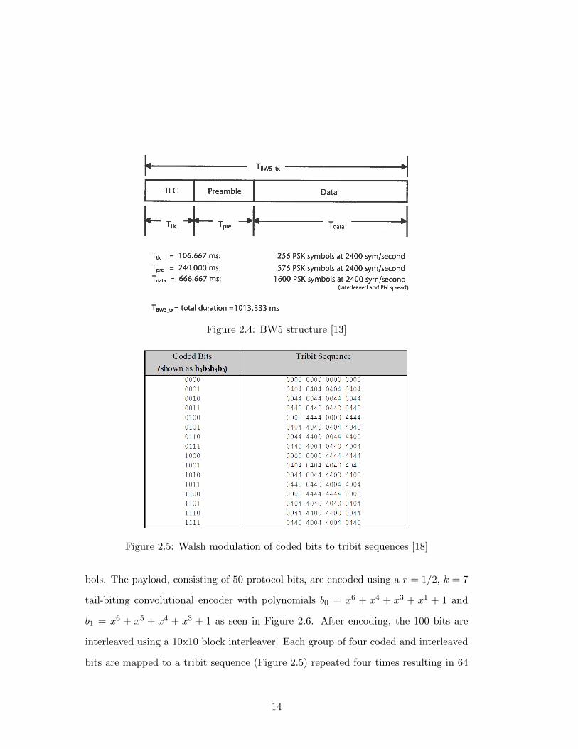
With the exception of BW2, data bits are modulated using an orthogonal Walsh
function. In groups of either four or two bits, the bits are mapped to 16 symbols of 0s
and 4s. For BW0, BW1, and BW5, the tribit sequences in Figure 2.5 are repeated four
times per four coded bits. For BW3, the sequences are not repeated and for BW1+ the
sequences are repeated twice. BW4 maps two bits (00,01,10,11) to only the first four
tribit sequences in Figure 2.5 and each sequence is repeated 80 times. The symbols are
then added modulo-8 to a pseudo-noise (PN) scrambling sequence which is essentially
the mapping of a BPSK signal to an 8-PSK signal prior to transmission. On the
demodulation side, this step involves descrambling an 8-PSK signal to a BPSK signal,
as shown in 2.3.
−1 −0.8 −0.6 −0.4 −0.2 0 0.2 0.4 0.6 0.8 1
−1
−0.8
−0.6
−0.4
−0.2
0
0.2
0.4
0.6
0.8
1
In−Phase
Quadrature
(a) Raw symbols out of equalizer
−1 −0.8 −0.6 −0.4 −0.2 0 0.2 0.4 0.6 0.8 1
−1
−0.8
−0.6
−0.4
−0.2
0
0.2
0.4
0.6
0.8
1
In−Phase
Quadrature
(b) Descrambled symbols
Figure 2.3: BW5 descrambling, SNR 30 dB
As an example, BW5 is discussed here in more detail. BW5 is an extended and
more robust verison of BW0, both of which are used for link setup at the beginning
of an ALE3G exchange. As shown in Figure 2.4, BW5 begins with a 256-symbol
TLC/AGC guard sequence, followed by 576 preamble symbols and 1600 payload sym-
13
Page 23
Figure 2.4: BW5 structure [13]
Figure 2.5: Walsh modulation of coded bits to tribit sequences [18]
bols. The payload, consisting of 50 protocol bits, are encoded using a r = 1/2, k = 7
tail-biting convolutional encoder with polynomials b0 = x
6 + x
4 + x
3 + x
1 + 1 and
b1 = x
6 + x
5 + x
4 + x
3 + 1 as seen in Figure 2.6. After encoding, the 100 bits are
interleaved using a 10x10 block interleaver. Each group of four coded and interleaved
bits are mapped to a tribit sequence (Figure 2.5) repeated four times resulting in 64
14
Page 24
Figure 2.6: BW5 convolutional encoder [21]
symbols for every four coded bits or 1600 total payload symbols; these symbols are
then component-wise modulo-8 added to a PN sequence and modulated onto an 1800
Hz carrier signal.
ALE3G is a complicated signal which includes many stages of redundancy due
to the challenges that must be overcome when transmitting through the ionosphere.
While redundancy is certainly helpful, the following chapters explain how adaptive
equalization and spatial diversity are also important tools that can be used to demod-
ulate and decode a reliable ALE3G signal.
15
Page 25
Chapter 3
Adaptive Equalization
3.1 Basics of Equalization
In a digital communications system, time dispersion is caused when data passes
through any frequency-selective channel. The amount of time dispersion and its cause
varies amongst transmission systems, but higher-data-rate applications such as those
described in Chapter 2 are most susceptible to delay spread. If the delay spread is
significant enough, pulses will be distorted such that zero-crossings will no longer be
periodic due to adjacent pulses overlapping. This phenomenon is called intersymbol
interference (ISI). To mitigate the e↵ects of ISI caused by a dispersive channel, an
equalizer can be used to model the inverse of the channel and restore pulses.
Because wireless communication channels typically vary in time, the filter coef-
ficients for the equalizer may also be time-varying. If this is the case, an adaptive
equalizer is necessary so that tap weights can be adjusted adaptively and the equal-
izer can best approximate the time-varying channel response inversion in real time.
Typically, there is a training sequence at the beginning of a transmission where known
symbols are sent and the equalizer adjusts its filter parameters by comparing its output
16
Page 26
to the known data. After the training sequence ends, the equalizer will leave training
mode and enter decision directed mode (also sometimes called tracking mode) where
the equalizer will have to make its own decisions based on what its learned from previ-
ous decisions made during training. Two adaptive filtering algorithms commonly used
in practice to adjust filter coe�cients are the least-mean-square (LMS) and recursive
least-squares (RLS) algorithms which are both described in the next two sections of
this chapter.
Equalizers can be linear or non-linear. Non-linear equalizers, such as decision
feedback equalizers (DFE) or maximum likelihood sequence estimation (MLSE), are
more complex to implement but are better at reducing noise enhancement. This the-
sis focuses on linear equalizers due to their simplicity but Chapter 7 mentions the
possibility of a DFE in future implementations of the joint spatial-temporal equalizer
algorithm. Linear equalizers can be implemented using either a transversal or lat-
tice structure, but the focus of this thesis is on transversal filters. Linear equalizers
can either be zero-forcing (ZF) equalizers or minimum mean square error (MMSE)
equalizers; ZF equalizers apply the inverse of the channel’s frequency response and
reduce ISI completely at the expense of enhancing noise, and MMSE equalizers aim
to minimize the error between the desired response and the actual response of the
equalizer. This thesis focuses on MMSE equalization.
It should be noted that a fractionally spaced equalizer is an equalizer that receives
an oversampled signal such that the output sample rate is K/T where K is an integer
corresponding to the number of input samples the equalizer received before producing
a single output sample. There are advantages to fractionally spaced equalizers when
the receiver does not know channel characteristics [19], however, as a simplification,
the focus of this work is on symbol-spaced equalization where the equalizer input and
17
Page 27
Figure 3.1: Symbol-spaced linear equalizer [16]
output sampling rates are equal.
Figure 3.1 shows the general structure for a symbol-spaced equalizer consisting of
a tapped delay line with L�1 delay elements, L tunable complex weights, an adaptive
weight setting, decision device, and error calculator.
To quantify equalizer performance, the mean squared error (MSE) is plotted
against each iteration of the algorithm in time, or, the number of training symbols.
The MSE is in terms of the Euclidean distance between the desired symbol and the
actual symbol. These curves are called learning curves because they show how quickly
the equalizer is learning the channel and the learning rate is referred to as the rate
of convergence. In addition to convergence time, the value of the MSE to which the
equalizer converges can be used to show how well an equalizer is doing. Another
useful way to check equalizer performance is to plot the output symbols. For a PSK
signal, a constellation where each phase is tightly clustered together will imply that
18
Page 28
the equalizer is working well.
3.2 LMS Filtering
The least-mean-square (LMS) algorithm is a type of stochastic gradient descent
algorithm [9]. Its feedback structure is a linear transversal (FIR) filter whose tap
weights are updated by an adaptive weight-control mechanism driven by minimizing
a cost function. For a Wiener filter, the cost function to be minimized is the mean
squared error:
J(n) = E[e(n)e⇤(n)] (3.1)
where the error signal e(n) is computed by comparing the filter output with a desired
response. If parameters are chosen appropriately, the LMS algorithm will converge
to an estimate of the optimum Wiener solution. Since the gradient vector rJ(n) at
each iteration of the steepest-descent algorithm is only an estimate, LMS will only
approach the optimal solution. Therefore, the cost function for LMS becomes the
instantaneous squared error:
J(n) = |e(n)|2 (3.2)
The LMS algorithm solves for the optimum value of the tap-weight vector w(n+1) that
minimizes the cost function J(n). Using the notation, approximations, and steepest
descent method results described in [9], we summarize the algorithm as follows. First,
the tap-weight vector is initialized:
w(0) = 0 (3.3)
19
Page 29
An L-by-1 tap-input vector at time n is given:
u(n) = [u(n), u(n� 1), ..., u(n� L+ 1)]T (3.4)
where L is the length of the adaptive transversal filter. Also given is the desired
response d(n) at time n. For an adaptive equalizer, the desired response is usually a
training sequence or probes known to the receiver. Next, an estimate of the tap-weight
vector at time n+ 1 is computed using the system:
e(n) = d(n)� wH(n)u(n) (3.5)
w(n+ 1) = w(n) + µu(n)e⇤(n) (3.6)
where µ is the step size parameter, a small positive quantity. At each iteration, the
LMS algorithm requires only 2L+ 1 multiplications; it is a simple but powerful tool.
3.3 RLS Filtering
The recursive least-squares (RLS) algorithm is another method used to recursively
estimate the tap-weight vector of a linear transversal filter. Unlike LMS, it is an
extension of the method of least squares rather than a stochastic gradient descent
approach. At the cost of computational complexity, the RLS algorithm converges
significantly faster (usually by an order of magnitude) than the LMS algorithm [9].
The RLS cost function to be minimized is:
"(n) =nX
i=1
�
n�i|e(i)|2 + ��
nkw(n)k2 (3.7)
20
Page 30
where the first term of the cost function is the sum of exponentially weighted error
squares. The exponential weighting is due to the forgetting factor �n�i where � is a
positive constant less than but close to 1 and serves as a measure of the algorithm’s
memory for past data. Similar to LMS, the error is defined as the di↵erence between
the desired response and the actual response of the filter:
e(i) = d(i)�wH(n)u(i) (3.8)
where the tap-input vector and tap-weight vectors are defined by
u(i) = [u(i), u(i� 1), ..., u(i� L+ 1)]T (3.9)
w(n) = [w0(n), w1(n), ..., wL�1(n)]T (3.10)
Note that only the tap weights remain fixed during the time interval. The second
term of the cost function is referred to as the regularizing term since the regularizing
parameter � is a positive real number included in the cost function for stability and
smoothing.
The RLS algorithm minimizes the cost function "(n) by using a reformulation
of the correlation matrix of the tap-input vector u(i) to compute the tap-weight
estimate w(n). In order to do this computation, the matrix inversion lemma is used
to calculate the inverse of the correlation matrix, P(n) = ��1(n). Using the notation,
approximations, method of least-squares results, and matrix inverse lemma results
described in [9], we summarize the algorithm as follows. In similar fashion to the
LMS algorithm, the tap-weight vector is first initialized in addition to the inverse
correlation matrix:
w(0) = 0 (3.11)
21
Page 31
P(0) = �
�1I (3.12)
At every time instant, the following equations are computed:
⇡(n) = P(n� 1)u(n) (3.13)
k(n) =⇡(n)
�+ uH(n)⇡(n)(3.14)
⇠(n) = d(n)� wH(n� 1)u(n) (3.15)
w(n) = w(n� 1) + k(n)⇠⇤(n) (3.16)
P(n) = �
�1P(n� 1)� �
�1k(n)uH(n)P(n� 1) (3.17)
where k(n) is the gain vector, ⇠(n) is the a priori estimation error computed during the
filtering operation, w(n) is the estimated tap-weight vector update, and the inverse
correlation matrix P(n) is used to update the gain vector. The biggest downfall of the
RLS algorithm is its computational complexity: it requires 2.5L2+4.5Lmultiplications
per iteration [6].
In summary, the LMS and RLS algorithms are powerful algorithms that can con-
trol the weight adaptation for adaptive equalization of signals blurred together from
ISI. The RLS algorithm converges much faster than LMS but is more complex to
implement. Both algorithms with varying parameters are used for the simulations
described later in Chapter 5.
22
Page 32
Chapter 4
Receiver Diversity
4.1 Basics of Diversity
In a fading channel, it is unlikely that multiple independent signal paths will
all experience a deep fade at the same time [6]. Therefore, it is desirable to create a
situation in which the same data is being sent over multiple independent paths because
adding these signals together results in a higher SNR than the SNR from a single path.
Independent fading paths can be obtained in a number of ways. Spatial diversity
refers to a situation where there are multiple transmit or receive antennas, where
maximum diversity gain is achieved by separating antennas by approximately one half-
wavelength if the antennas are omnidirectional [6]. Other diversity techniques include
polarization diversity (where two antennas have vertical and horizontal polarizations),
directional diversity (by use of directional antennas that specify a particular receive
beamwidth), and frequency diversity (by transmitting at di↵erent carrier frequencies).
The focus of this thesis is on receiver spatial diversity so the combining techniques
described in the following sections will be discussed in such a context. Spatial diversity
was chosen because of the popularity of multi-channel HF receivers.
23
Page 33
4.2 Combining Techniques
The general structure for a linear combiner is illustrated in Figure 4.1. The com-
plex weights ↵i are used to scale each of the received signals riej✓i
s(t) where s(t) is
the transmitted signal, ri is the amplitude of the signal at the ith branch, and ✓i is the
phase of the signal at the ith branch. Depending on the combining technique, ↵i will
take on di↵erent forms. For example, if ↵i is zero-valued at all but one branch, the
output results from selection combining or threshold combining; if ↵i is nonzero for
more than one branch, the output results from maximal-ratio combining or equal-gain
combining.
Figure 4.1: Linear combiner [6]
Selection combining (SC) is a combining technique where the the branch with the
highest SNR is the one that is output, and the other M�1 branches are multiplied by
↵i = 0 and disregarded. For SC, the SNR gain increases with an increasing number
of diversity branches but the relationship is not linear; the biggest gain occurs when
24
Page 34
increasing from one branch to two [6]. If a system is continuously transmitting, the
SNR at each branch will change so each branch requires its own receiver to monitor
these changes. However, if threshold combining (TC) is used instead, only one receiver
is needed to scan each branch. The receiver selects the first branch whose SNR is above
a specified threshold and switches to scan another branch as soon as the SNR falls
below the threshold.
To achieve better SNR gain, maximal-ratio combining (MRC) can be used to sum
weighted versions of all the branches together. In order to allow coherent detection,
the phase ✓i must be removed from the received signals through multiplication by
↵i = aie�j✓i where the gain of branch ai is real. This is called co-phasing and is
necessary when more than one branch is used in combining so that each signal has
the same phase and there is no constructive or destructive interference. The resulting
combiner SNR is equal to the sum of the SNRs on each branch. Thus, the array
gain increases linearly with M [6]. Without knowing the SNR on each branch, MRC
cannot be performed and instead equal gain combining (EGC) can be used to sum all
of the branches together. For EGC, co-phasing is again necessary but ↵i = e
�j✓i since
ai = 1 and each branch is equally weighted. Equal gain combining does not work as
e↵ectively as MRC since stronger signals are not weighted more heavily however the
di↵erence between EGC and MRC performance is typically less than 1 dB [6].
25
Page 35
Chapter 5
Joint Spatial-Temporal
Equalization
5.1 System Model
Building upon the previous work and theory discussed in the earlier chapters of this
thesis, a joint spatial-temporal equalizer is developed to jointly optimize the combiner
weights and equalizer coe�cients for a multi-channel receiver. A synthetic ALE3G
waveform is transmitted through a Watterson channel simulator and received using a
uniform linear array (ULA). The signal received at each branch is then sampled every
symbol prior to combining and equalizing.
26
Page 36
∑
𝑧 𝑧 𝑧
𝑤∗(𝑛) 𝑤∗(𝑛) 𝑤∗ (𝑛) 𝑤∗(𝑛) 𝑤∗(𝑛)
∑ ∑ ∑ ∑
∑ Adaptive weight-control mechanism
𝑟 𝑒 𝑠(𝑡)
𝛼
𝑢(𝑛) 𝑢(𝑛 − 1) 𝑢(𝑛 − 2) 𝑢(𝑛 − 𝐿 + 1)
𝑦(𝑛)
𝑑(𝑛)
𝑒(𝑛) −
+
𝛼 𝛼
𝑟 𝑒 𝑠(𝑡) 𝑟 𝑒 𝑠(𝑡)
Figure 5.1: Linear combiner followed by single-channel equalizer
27
Page 37
Adaptive weight-control mechanism
𝑦(𝑛)
𝑑(𝑛)
𝑒(𝑛) −
+
𝑟 𝑒 𝑠(𝑡)
𝛼 𝛼 𝛼
𝑟 𝑒 𝑠(𝑡) 𝑟 𝑒 𝑠(𝑡)
𝑧 𝑧 𝑧
𝑐 ,∗ (𝑛)
∑ ∑ ∑ ∑
𝑣 (𝑛)
𝑐 ,∗ (𝑛) 𝑐 ,∗ (𝑛) 𝑐 ,∗ (𝑛) 𝑐 ,
∗ (𝑛)
𝑣 (𝑛 − 1) 𝑣 (𝑛 − 2) 𝑣 (𝑛 − 𝐿𝑀 + 1)
𝑧 𝑧 𝑧
𝑐 ,∗ (𝑛)
∑ ∑ ∑ ∑
𝑣 (𝑛)
𝑐 ,∗ (𝑛) 𝑐 ,∗ (𝑛) 𝑐 ,∗ (𝑛) 𝑐 ,
∗ (𝑛)
𝑣 (𝑛 − 1) 𝑣 (𝑛 − 2) 𝑣 (𝑛 − 𝐿𝑀 + 1)
𝑧 𝑧 𝑧
𝑐 ,∗ (𝑛)
∑ ∑ ∑ ∑
𝑣 (𝑛)
𝑐 ,∗ (𝑛) 𝑐 ,∗ (𝑛) 𝑐 ,∗ (𝑛) 𝑐 ,
∗ (𝑛)
𝑣 (𝑛 − 1) 𝑣 (𝑛 − 2) 𝑣 (𝑛 − 𝐿𝑀 + 1)
∑
∑
∑
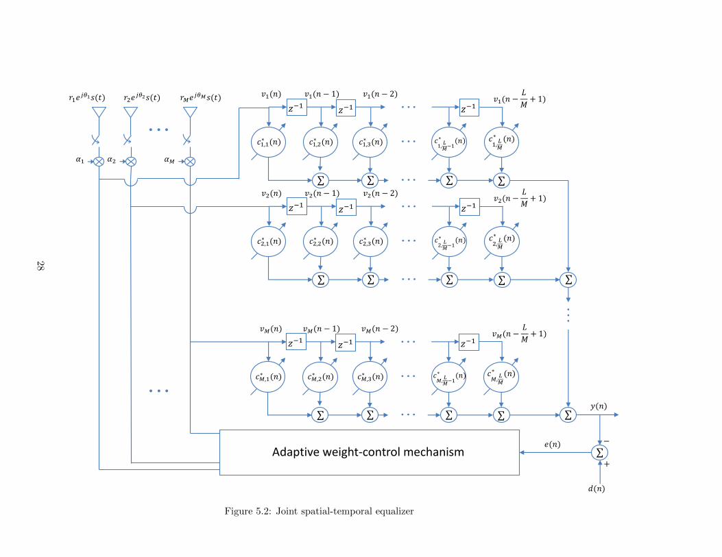
Figure 5.2: Joint spatial-temporal equalizer
28
Page 38
Before deriving the joint spatial-temporal equalizer system model, it is important
to understand the two-step system model of a linear combiner followed by equaliza-
tion shown in Figure 5.1. The sampled received signal at the ith branch is given
by riej✓i
s(n) where the only di↵erence between this model and the linear combiner
introduced in Chapter 4 is that the signals in this model are sampled every symbol.
After being scaled by the combiner weights, the signal at the ith branch becomes
airis(n) regardless of the combining method being MRC or EGC. After each of these
signals are summed together, the combiner output is the input to a single-channel
linear adaptive equalizer. The complex output of the equalizer y(n) is demodulated
and decoded as per the ALE3G standard as described in Chapter 2.
The joint spatial-temporal equalizer is di↵erent from the two-step system model
previously discussed because it requires only one step to perform both temporal and
spatial processing. The system model is shown in 5.2. For simplicity, we will only
derive the LMS case, but the same derivation can be extended for the RLS case. The
signals received at each antenna are passed through a tapped-delay line having L/M
delay elements, where M is the total number of diversity branches and L is an integer:
vi(n) = [vi(n), vi(n� 1), ..., vi(n� L/M + 1)] (5.1)
and a composite input vector of length L is constructed:
u(n) = [v1(n),v2(n), ...,vM (n)]T (5.2)
The combiner weights at each branch are given by
ci(n) = [ci,1(n), ci,2(n), ..., ci,L/M (n)]T (5.3)
29
Page 39
which are initialized to ci(n) = 0 at the start of the algorithm. Each of these combiner
weights are concatenated together to create a composite tap-weight vector of length
L:
wH(n) = [cH1 (n), cH2 (n), ..., cHM (n)] (5.4)
and the filter output is given by
y(n) = wH(n)u(n) (5.5)
The error signal e(n) and estimated tap-weight vector update w(n + 1) are given in
Chapter 3 (Equations 3.5 and 3.6) and reproduced here for convenience:
e(n) = d(n)� y(n)
w(n+ 1) = w(n) + µu(n)e⇤(n)
Note that there is a restriction on the selection of filter length L given M diversity
branches; Lmust be a multiple ofM . This constraint exists for ease of implementation
and so that the same amount of spatial information from each branch is weighted
and equalized. After symbol decisions are made, the waveform is demodulated and
decoded.
5.2 Simulation Details
An ALE3G BW5 payload of 50 bits is formed into PSK symbols as described
in Chapter 2. The symbols are then upsampled by an upsampling factor of four
samples per symbol and filtered by a raised cosine pulseshaping filter with a stopband
attenuation of 60 dB and a rollo↵ factor of 0.5. The modulated symbols are then
30
Page 40
transmitted at 9600 symbols per second (the baud rate upsampled by four) through the
ionosphere simulated using the Watterson model with mid-latitude quiet conditions:
two paths, 0.1 Hz Doppler spread, 0.5 ms relative path delay, path gains of 0 dB
and -1 dB, various SNR values ranging from -20 dB to 35 dB, and specified angles of
arrival for each signal path.
A simulated array manifold is created for a ULA having between one and four
isotropic elements spaced one half-wavelength apart. After the signal is received by
the antenna array, it is downsampled and aligned in time according to its baud rate.
For both the combiner followed by single-channel equalizer and joint spatial-temporal
equalizer cases, the same equalizer parameters are used to give valid comparisons.
Tap weights are initialized to all zeros, the total number of taps varies across simu-
lations and ranges from 12 to 48, the step size (LMS) varies from 0.01 to 0.40, the
regularization parameter (RLS) is 0.01, the forgetting factor (RLS) ranges from 0.85
to 0.99. After equalization, the symbols are demodulated and decoded according to
the ALE3G BW5 standard and results are compared, evaluated, and discussed.
31
Page 41
Chapter 6
Experimental Results
6.1 Introduction
The joint spatial-temporal equalizer was compared against two other diversity
receiver structures: an EGC followed by a single-channel (temporal) equalizer, and
an MRC followed by a single-channel equalizer. It is found that EGC and MRC
performance are comparable for the simulations performed so for ease of legibility, the
results presented in the following sections compare the joint spatial-temporal equalizer
to only one other receiver structure. The next two sections present results for equalizer
convergence and overall system performance through demodulation and decoding.
6.2 Equalizer Convergence
The joint spatial-temporal equalizer was compared against the single-channel equal-
izer following a linear combiner. For various SNRs, total number of tap weights, and
step size µ (for LMS) or forgetting factor � (for RLS), the convergence times and
MSEs (where the error is the Euclidean distance between constellation points) were
32
Page 42
recorded for four branches of diversity after averaging 20 independent trials and are
shown in Table 6.1 and Table 6.2 where SCE refers to the single-channel equalizer
after combining using an EGC and JSTE refers to the joint spatial-temporal equal-
izer. Convergence times are in terms of number of training symbols (out of 832) and
are calculated by choosing a threshold and selecting the last training symbol that
remained under the threshold as the point of convergence. The MSE was recorded as
the error at the last training symbol. If neither equalizer converged before the last
training symbol, convergence was not recorded. These tables are presented to help
the reader understand the e↵ect of di↵erent parameters on equalization. It should be
noted that for many combinations of parameters, the equalizers converged but only
after training mode ended; the results from these experiments were not recorded ex-
cept for the LMS cases when the joint spatial-temporal equalizer converged during
training but the single-channel equalizer did not.
There are only three runs of the LMS convergence simulations shown in Table 6.1
where the MSE for SCE is lower then the MSE for JSTE and not a single case where
the SCE converged faster than the STE. There are also only three runs from Table 6.2
where the MSE was lower for SCE than JSTE and again no cases of faster convergence.
For both the RLS and LMS algorithms, the joint spatial-temporal equalizer learns
its tap weights faster than the single-channel equalizer and in general more closely
approaches the optimal weights. This is an advantage especially for when there are
short training sequences without any probes such as those seen in ALE3G BW0, BW1,
BW3, and BW5.
For selected experiments, learning curves for 20 iterations and 8-PSK constellations
for a single iteration are presented to o↵er side-by-side comparisons between the joint
spatial-temporal equalizer and the combiner followed by single-channel equalizer. The
33
Page 43
Table 6.1: Equalizer convergence comparisons, LMS
µ Taps SNR (dB) Conv., SCE Conv., JSTE MSE, SCE MSE, JSTE0.05 24 10 – 570 0.0185 0.00170.05 24 20 – 270 0.0550 0.00090.05 24 35 – 733 0.0298 0.00040.05 36 10 – 553 0.0262 0.00500.05 36 20 – 727 0.0507 0.00030.10 12 10 – 130 0.0103 0.00590.10 12 20 – 339 0.0295 0.01010.10 24 10 – 266 0.0242 0.01380.10 24 20 – 225 0.0189 0.00090.10 36 10 – 714 0.0044 0.01620.10 36 20 – 523 0.0264 0.00020.10 48 10 – 254 0.0272 0.00710.10 48 20 – 400 0.0121 0.00030.15 12 10 – 551 0.0316 0.00810.15 12 20 – 784 0.0240 0.00180.15 24 10 – 95 0.0234 0.00890.15 24 20 774 335 0.0028 0.00040.15 36 10 – 417 0.0123 0.01140.15 36 20 – 546 0.0174 0.00180.20 12 10 – 227 0.0037 0.00650.20 12 20 389 296 0.0030 0.00040.20 24 20 719 136 0.0054 0.00080.20 36 10 – 127 0.0374 0.00520.20 36 20 792 274 0.0187 0.03170.30 12 10 – 73 0.0072 0.00630.30 12 20 749 616 0.0100 0.00040.40 12 10 144 58 0.0387 0.01010.40 12 20 351 205 0.0160 0.0008
learning curves are a way to visualize much of the same data presented in Table 6.1 and
Table 6.2 and the symbol constellations show further a�rmation that the equalizer is
doing a good job at making symbol decisions. The symbol constellations tend to be
more closely clustered around correct symbols for the joint spatial-temporal equalizer
symbols. It should be noted that the constellations show all of the symbols in a
34
Page 44
Table 6.2: Equalizer convergence comparisons, RLS
� Taps SNR (dB) Conv., SCE Conv., JSTE MSE, SCE MSE, JSTE0.99 12 20 502 476 0.0087 0.00020.99 24 10 559 379 0.0316 0.00620.99 24 20 600 446 0.0173 0.00070.99 36 10 556 376 0.0139 0.00280.99 36 20 693 586 0.0073 0.00940.99 48 10 589 430 0.0325 0.00360.99 48 20 693 587 0.0013 0.00120.95 12 10 275 110 0.0258 0.00760.95 12 20 791 679 0.0108 0.00100.95 24 10 123 76 0.0116 0.01820.95 24 20 143 137 0.0278 0.00200.95 36 10 123 76 0.0116 0.01820.95 36 20 143 137 0.0278 0.00200.95 48 20 208 123 0.0045 0.00090.90 12 10 58 54 0.0256 0.00170.90 12 20 69 69 0.0272 0.00090.90 24 10 69 51 0.0489 0.00610.90 24 20 79 74 0.0193 0.00370.90 36 10 86 51 0.0558 0.02670.90 36 20 81 67 0.0067 0.00120.90 48 10 109 51 0.0515 0.02950.90 48 20 96 62 0.0074 0.00490.85 12 10 70 33 0.0376 0.01240.85 12 20 54 46 0.0810 0.00140.85 24 10 54 37 0.0692 0.02600.85 24 20 192 43 0.0157 0.00520.85 24 30 58 50 0.0227 0.00020.85 36 20 66 49 0.0109 0.00240.85 48 20 87 47 0.0205 0.01480.85 48 30 96 53 0.0004 0.0003
transmission including the transient period before the equalizers converged.
35
Page 45
−1 −0.8 −0.6 −0.4 −0.2 0 0.2 0.4 0.6 0.8 1
−1
−0.8
−0.6
−0.4
−0.2
0
0.2
0.4
0.6
0.8
1
In−Phase
Quadrature
(a) EGC + single-channel equalizer
−1 −0.8 −0.6 −0.4 −0.2 0 0.2 0.4 0.6 0.8 1
−1
−0.8
−0.6
−0.4
−0.2
0
0.2
0.4
0.6
0.8
1
In−Phase
Quadrature
(b) Joint spatial-temporal equalizer
Figure 6.1: Equalized symbols: 24 taps, RLS(0.99), SNR 20 dB, 4 diversity branches
0 100 200 300 400 500 600 700 8000
0.2
0.4
0.6
0.8
1
1.2
1.4
Mea
n Sq
uare
d Er
ror
Training Symbols
Joint spatial−temporal equalizerMRC + single−channel equalizer
Figure 6.2: Learning curves: 24 taps, RLS(0.99), SNR 20 dB, 4 diversity branches
36
Page 46
−1 −0.8 −0.6 −0.4 −0.2 0 0.2 0.4 0.6 0.8 1
−1
−0.8
−0.6
−0.4
−0.2
0
0.2
0.4
0.6
0.8
1
In−Phase
Quadrature
(a) EGC + single-channel equalizer
−1 −0.8 −0.6 −0.4 −0.2 0 0.2 0.4 0.6 0.8 1
−1
−0.8
−0.6
−0.4
−0.2
0
0.2
0.4
0.6
0.8
1
In−Phase
Quadrature
(b) Joint spatial-temporal equalizer
Figure 6.3: Equalized symbols: 24 taps, RLS(0.95), SNR 20 dB, 4 diversity branches
0 100 200 300 400 500 600 700 8000
0.2
0.4
0.6
0.8
1
1.2
1.4
Mea
n Sq
uare
d Er
ror
Training Symbols
Joint spatial−temporal equalizerMRC + single−channel equalizer
Figure 6.4: Learning curves: 24 taps, RLS(0.95), SNR 20 dB, 4 diversity branches
37
Page 47
−1 −0.8 −0.6 −0.4 −0.2 0 0.2 0.4 0.6 0.8 1
−1
−0.8
−0.6
−0.4
−0.2
0
0.2
0.4
0.6
0.8
1
In−Phase
Quadrature
(a) EGC + single-channel equalizer
−1 −0.8 −0.6 −0.4 −0.2 0 0.2 0.4 0.6 0.8 1
−1
−0.8
−0.6
−0.4
−0.2
0
0.2
0.4
0.6
0.8
1
In−Phase
Quadrature
(b) Joint spatial-temporal equalizer
Figure 6.5: Equalized symbols: 12 taps, RLS(0.95), SNR 10 dB, 4 diversity branches
0 100 200 300 400 500 600 700 8000
0.2
0.4
0.6
0.8
1
1.2
1.4
Mea
n Sq
uare
d Er
ror
Training Symbols
Joint spatial−temporal equalizerMRC + single−channel equalizer
Figure 6.6: Learning curves: 12 taps, RLS(0.95), SNR 10 dB, 4 diversity branches
38
Page 48
−1 −0.8 −0.6 −0.4 −0.2 0 0.2 0.4 0.6 0.8 1
−1
−0.8
−0.6
−0.4
−0.2
0
0.2
0.4
0.6
0.8
1
In−Phase
Quadrature
(a) EGC + single-channel equalizer
−1 −0.8 −0.6 −0.4 −0.2 0 0.2 0.4 0.6 0.8 1
−1
−0.8
−0.6
−0.4
−0.2
0
0.2
0.4
0.6
0.8
1
In−Phase
Quadrature
(b) Joint spatial-temporal equalizer
Figure 6.7: Equalized symbols: 12 taps, RLS(0.90), SNR 20 dB, 4 diversity branches
0 100 200 300 400 500 600 700 8000
0.2
0.4
0.6
0.8
1
1.2
1.4
Mea
n Sq
uare
d Er
ror
Training Symbols
Joint spatial−temporal equalizerMRC + single−channel equalizer
Figure 6.8: Learning curves: 12 taps, RLS(0.90), SNR 20 dB, 4 diversity branches
39
Page 49
−1 −0.8 −0.6 −0.4 −0.2 0 0.2 0.4 0.6 0.8 1
−1
−0.8
−0.6
−0.4
−0.2
0
0.2
0.4
0.6
0.8
1
In−Phase
Quadrature
(a) EGC + single-channel equalizer
−1 −0.8 −0.6 −0.4 −0.2 0 0.2 0.4 0.6 0.8 1
−1
−0.8
−0.6
−0.4
−0.2
0
0.2
0.4
0.6
0.8
1
In−Phase
Quadrature
(b) Joint spatial-temporal equalizer
Figure 6.9: Equalized symbols: 36 taps, LMS(0.05), SNR 10 dB, 4 diversity branches
0 100 200 300 400 500 600 700 8000
0.2
0.4
0.6
0.8
1
1.2
1.4
Mea
n Sq
uare
d Er
ror
Training Symbols
Joint spatial−temporal equalizerMRC + single−channel equalizer
Figure 6.10: Learning curves: 36 taps, LMS(0.05), SNR 10 dB, 4 diversity branches
40
Page 50
−1 −0.8 −0.6 −0.4 −0.2 0 0.2 0.4 0.6 0.8 1
−1
−0.8
−0.6
−0.4
−0.2
0
0.2
0.4
0.6
0.8
1
In−Phase
Quadrature
(a) EGC + single-channel equalizer
−1 −0.8 −0.6 −0.4 −0.2 0 0.2 0.4 0.6 0.8 1
−1
−0.8
−0.6
−0.4
−0.2
0
0.2
0.4
0.6
0.8
1
In−Phase
Quadrature
(b) Joint spatial-temporal equalizer
Figure 6.11: Equalized symbols: 36 taps, LMS(0.10), SNR 20 dB, 4 diversity branches
0 100 200 300 400 500 600 700 8000
0.2
0.4
0.6
0.8
1
1.2
1.4
Mea
n Sq
uare
d Er
ror
Training Symbols
Joint spatial−temporal equalizerMRC + single−channel equalizer
Figure 6.12: Learning curves: 36 taps, LMS(0.10), SNR 20 dB, 4 diversity branches
41
Page 51
−1 −0.8 −0.6 −0.4 −0.2 0 0.2 0.4 0.6 0.8 1
−1
−0.8
−0.6
−0.4
−0.2
0
0.2
0.4
0.6
0.8
1
In−Phase
Quadrature
(a) EGC + single-channel equalizer
−1 −0.8 −0.6 −0.4 −0.2 0 0.2 0.4 0.6 0.8 1
−1
−0.8
−0.6
−0.4
−0.2
0
0.2
0.4
0.6
0.8
1
In−PhaseQuadrature
(b) Joint spatial-temporal equalizer
Figure 6.13: Equalized symbols: 12 taps, LMS(0.15), SNR 20 dB, 4 diversity branches
0 100 200 300 400 500 600 700 8000
0.2
0.4
0.6
0.8
1
1.2
1.4
Mea
n Sq
uare
d Er
ror
Training Symbols
Joint spatial−temporal equalizerMRC + single−channel equalizer
Figure 6.14: Learning curves: 12 taps, LMS(0.15), SNR 20 dB, 4 diversity branches
42
Page 52
−1 −0.8 −0.6 −0.4 −0.2 0 0.2 0.4 0.6 0.8 1
−1
−0.8
−0.6
−0.4
−0.2
0
0.2
0.4
0.6
0.8
1
In−Phase
Quadrature
(a) EGC + single-channel equalizer
−1 −0.8 −0.6 −0.4 −0.2 0 0.2 0.4 0.6 0.8 1
−1
−0.8
−0.6
−0.4
−0.2
0
0.2
0.4
0.6
0.8
1
In−Phase
Quadrature
(b) Joint spatial-temporal equalizer
Figure 6.15: Equalized symbols: 12 taps, LMS(0.40), SNR 20 dB, 4 diversity branches
0 100 200 300 400 500 600 700 8000
0.5
1
1.5
Mea
n Sq
uare
d Er
ror
Training Symbols
Joint spatial−temporal equalizerMRC + single−channel equalizer
Figure 6.16: Learning curves: 12 taps, LMS(0.40), SNR 20 dB, 4 diversity branches
43
Page 53
6.3 Receiver Performance
In order to measure how well the entire systems are performing through demodu-
lation and decoding, bit error rates (BERs) are plotted against various signal-to-noise
ratios (SNRs) for all three diversity receivers. Each simulation is averaged over 1000
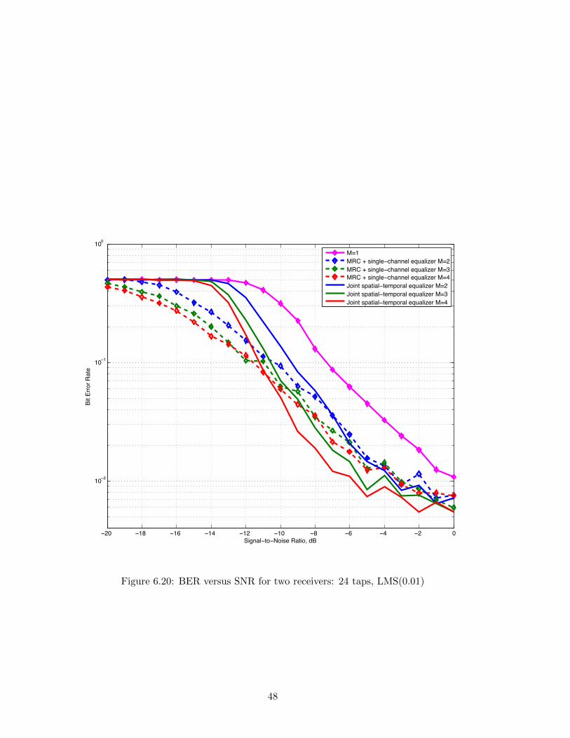
independent trials and the results are presented in Figures 6.17, 6.18, 6.19, 6.20.
Figure 6.17 shows the BER for SNRs of -20 dB to 5 dB for two 12-tap RLS
equalizers with forgetting factors of 0.99. This combination of parameters performs
the best overall for all three receivers at low SNRs, but the EGC receiver is left
out of the plot for clarity since it performs similarly to MRC; this is also the case
for subsequent simulations. With increasing the number of equalizer filter taps but
holding other parameters the same, performance across all receivers drops slightly
because there are more weights to be learned. The joint spatial-temporal equalizer
has less than 1 dB improvement for two branches of diversity, 1.5 dB improvement
for three branches, and 2 dB improvement for four branches.
Figure 6.18 shows the BER for SNRs of -10 dB to 20 dB for two 12-tap RLS
equalizers with forgetting factors of 0.95. Decreasing the forgetting factor from 0.99
results in good performance but for a higher range of SNRs. This figure more clearly
shows the performance gain of the joint spatial-temporal equalizer; there is a 6 dB
improvement for two branches of diversity, 9 dB improvement for three branches,
and 10 dB improvement for four branches. Reducing the forgetting factor to 0.90
as shown in Figure 6.19 illustrates an even greater performance gap between the
joint spatial-temporal equalizer and the MRC followed by single-channel equalizer.
However, overall performance drops slightly for the JSTE and drastically for the
other receivers. The majority of the LMS simulations did not work as well as the RLS
equalizers. As seen in Figure 6.20, the MRC receiver performs better than JSTE at the
44
Page 54
lowest SNRs. At -8.5 dB, the JSTE for two diversity branches begins to outperform
but not significantly. For three diversity branches, the JSTE begins to perform better
than MRC at around -10 dB and shows a 1 dB improvement. At -11 dB, the JSTE
for four diversity branches begins to outperform and reaches an improvement of 2 dB.
−20 −15 −10 −5 0 5
10−2
10−1
100
Signal−to−Noise Ratio, dB
Bit E
rror R
ate
M=1MRC + single−channel equalizer M=2MRC + single−channel equalizer M=3MRC + single−channel equalizer M=4Joint spatial−temporal equalizer M=2Joint spatial−temporal equalizer M=3Joint spatial−temporal equalizer M=4
Figure 6.17: BER versus SNR for two receivers: 12 taps, RLS(0.99)
45
Page 55
−10 −5 0 5 10 15 20
10−2
10−1
100
Signal−to−Noise Ratio, dB
Bit E
rror R
ate
M=1MRC + single−channel equalizer M=2MRC + single−channel equalizer M=3MRC + single−channel equalizer M=4Joint spatial−temporal equalizer M=2Joint spatial−temporal equalizer M=3Joint spatial−temporal equalizer M=4
Figure 6.18: BER versus SNR for two receivers: 12 taps, RLS(0.95)
46
Page 56
−5 0 5 10 15 20
10−2
10−1
100
Signal−to−Noise Ratio, dB
Bit E
rror R
ate
M=1MRC + single−channel equalizer M=2MRC + single−channel equalizer M=3MRC + single−channel equalizer M=4Joint spatial−temporal equalizer M=2Joint spatial−temporal equalizer M=3Joint spatial−temporal equalizer M=4
Figure 6.19: BER versus SNR for two receivers: 12 taps, RLS(0.90)
47
Page 57
−20 −18 −16 −14 −12 −10 −8 −6 −4 −2 0
10−2
10−1
100
Signal−to−Noise Ratio, dB
Bit E
rror R
ate
M=1MRC + single−channel equalizer M=2MRC + single−channel equalizer M=3MRC + single−channel equalizer M=4Joint spatial−temporal equalizer M=2Joint spatial−temporal equalizer M=3Joint spatial−temporal equalizer M=4
Figure 6.20: BER versus SNR for two receivers: 24 taps, LMS(0.01)
48
Page 58
Chapter 7
Conclusions and Future Work
The joint spatial-temporal equalizer outperformed linear combiners followed by
single-channel equalization under many di↵erent conditions in terms of equalizer con-
vergence times, equalizer MSE, and overall BER, especially at low SNRs. By jointly
combining and equalizing, there is no need to compute the channel gain or perform co-
phasing of received signals. For an SDR framework that uses a dataflow architecture,
this is advantageous since the receiver requires less software components to perform
combining and equalizing. The proposed algorithm is easily scalable for multiple input
channels if a software defined receiver already implements a single-channel equalizer.
Possible avenues for future work include implementing and testing di↵erent adap-
tive algorithms for linear equalizer tap-weight estimation, using fractionally spaced
equalization instead of symbol-spaced, or using a nonlinear equalizer such as a DFE.
Another avenue to explore for future work is to treat the equalizer as a classifier and
use machine learning algorithms to learn the combiner and equalizer weights for a
spatial-temporal equalizer. Lastly, rewriting the code in python and C++ and testing
the algorithm with live multi-channel data on a Southwest Research Institute system
49
Page 59
is another potential opportunity for future work.
50
Page 60
Appendix A
MATLAB Code
The following Matlab functions were used for the simulations in this thesis.
The script ALE3G Watterson EqCompare calls the functions ALE3Gmod, ALE3Gdemod,
equalizer, and ChannelSimulator v5, an HF channel simulator modified from one
originally written by Ryan Casey of Southwest Research Institute.
A.1 ALE3G Signal Generator
1 function [msg,tx,upsamp,syms] = ALE3Gmod(BW)
2 % ALE3G modulation
3 % 8�PSK, 1800 Hz carrier, 2400 baud
4
5 % parameters
6 %Fc = 1800; % carrier frequency, Hz
7 %baud = 2400; % symbols per second
8 upsamp = 4; % upsample factor, samples per symbol
9 %Fs = upsamp*baud; % sampling frequency, Hz
10
11 % TLC/AGC guard sequence, 256 syms
12 tlc = textread('tlcagc.txt','%n');
13
14 switch BW
51
Page 61
15 case '0'
16 bits = 26; % number of payload bits
17 constlen = 7; % encoder constraint length
18 codegen = [133 171]; % generator polynomials in octal
19 row = 4; col = 13; % interleaving matrix
20 base = 16; % for mapping bits to syms
21 chip = 64;
22 pn = 'PNseqBW0.txt'; % pn scrambling sequence
23 pre = 'pre0.txt'; % preamble
24 payload = 832; % number of payload syms
25 case '1'
26 bits = 48;
27 constlen = 9;
28 codegen = [711 663 557];
29 row = 16; col = 9;
30 base = 16;
31 chip = 64;
32 pn = 'PNseqBW1.txt';
33 pre = 'pre1.txt';
34 payload = 2304;
35 case '1+'
36 bits = 51;
37 constlen = 7;
38 codegen = [133 171];
39 puncpat = [1,1,0];
40 base = 16;
41 chip = 32;
42 pn = 'PNseqBW1.txt';
43 tlc = tlc(1:192);
44 pre = 'pre1plus.txt';
45 payload = 544;
46 case '2' % make add'l cases for variable lengths
47 constlen = 8;
48 codegen = [];
49 pn = 'PNseqBW2.txt';
50 tlc = tlc(1:240);
51 pre = 'pre2.txt';
52 %payload = 2880; %5760,11520,23040, 304+(n*960), n=3,6,12,24
53 case '3' % make add'l cases for variable lengths
54 constlen = 7;
55 codegen = [];
56 base = 16;
57 chip = 16;
52
Page 62
58 pn = 'PNseqBW3.txt';
59 tlc = 0;
60 pre = 'pre3.txt';
61 %payload = 2304; %4352,8448,16640
62 case '4'
63 bits = 2;
64 base = 4;
65 chip = 1280;
66 pn = 'PNseqBW4.txt';
67 payload = 1280;
68 case '5'
69 %crc = []; % 8�bit CRC
70 bits = 50;
71 constlen = 7;
72 codegen = [133 171];
73 row = 10; col = 10;
74 base = 16;
75 chip = 64;
76 pn = 'PNseqBW5.txt';
77 pre = 'pre5.txt';
78 payload = 1600;
79 end
80
81 % binary data stream
82 msg = round(rand(bits,1));
83 % crc = CRC BW5(msg,poly,etc.)
84 %msg = cat(1,msg,crc);
85
86 if ˜strcmp(BW,'4')
87 % FEC
88 init state = msg(end:�1:bits�constlen+2); % last constlen�1 bits
89 init state = bin2dec(num2str(init state'));
90 trellis = poly2trellis(constlen,codegen);
91 if ˜strcmp(BW,'1+')
92 coded = convenc(msg,trellis,init state);
93 else
94 coded = convenc(msg,trellis,puncpat,init state);
95 end
96 % CHECK: viterbi decode
97 % tblen = 5*constlen;
98 % vit = vitdec([coded;coded],trellis,tblen,'trunc','hard');
99 % vit = vit(bits+1:end); % check: is vit same as msg?
100 % sum(vit == msg) % should = 50 for BW5
53
Page 63
101
102 if ˜strcmp(BW,'1+')
103 % interleave
104 deintrlvd = reshape(coded,row,col);
105 intrlvd = reshape(deintrlvd',row*col,1);
106 % CHECK: deinterleave
107 % i = reshape(intrlvd,col,row)';
108 % codedBits = reshape(i,col*row,1);
109 % sum(codedBits == coded) % should = 100 for BW5
110
111 % base change
112 bc = reshape(intrlvd,log2(base),row*col/log2(base))';
113 else % BW 1+ � yes FEC but no interleaving
114 bc = reshape(coded,log2(base),length(coded)/log2(base))';
115 end
116 else % BW 4 � no FEC or interleaving
117 bc = reshape(msg,log2(base),bits/log2(base))';
118 end
119 corr = bin2dec(num2str(bc));
120
121 % walsh modulation
122 if strcmp(BW,'4')
123 % Table C�XVIII, mapped to complex [0,4] ��> [1,�1]124 tribitSeq = zeros(chip,4);
125 tribitSeq(:,1) = ones(chip,1); % 00
126 tribitSeq(:,2) = repmat([1;�1;1;�1],chip/4,1); % 01
127 tribitSeq(:,3) = repmat([1;1;�1;�1],chip/4,1); % 10
128 tribitSeq(:,4) = repmat([1;�1;�1;1],chip/4,1); % 11
129 else
130 % Table C�VIII, mapped to complex [0,4] ��> [1,�1]131 tribitSeq = zeros(chip,16);
132 tribitSeq(:,1) = ones(chip,1); % 0000
133 tribitSeq(:,2) = repmat([1;�1;1;�1],chip/4,1); % 0001
134 tribitSeq(:,3) = repmat([1;1;�1;�1],chip/4,1); % 0010
135 tribitSeq(:,4) = repmat([1;�1;�1;1],chip/4,1); % 0011
136 tribitSeq(:,5) = repmat([1;1;1;1;�1;�1;�1;�1],chip/8,1); % 0100
137 tribitSeq(:,6) = repmat([1;�1;1;�1;�1;1;�1;1],chip/8,1); % 0101
138 tribitSeq(:,7) = repmat([1;1;�1;�1;�1;�1;1;1],chip/8,1); % 0110
139 tribitSeq(:,8) = repmat([1;�1;�1;1;�1;1;1;�1],chip/8,1); % 0111
140 tribitSeq(:,9) = repmat([ones(8,1);�1*ones(8,1)],chip/16,1); % 1000
141 tribitSeq(:,10) = repmat([repmat([1;�1],4,1);repmat([�1;1],4,1)],...142 chip/16,1); % 1001
143 tribitSeq(:,11) = repmat([1;1;�1;�1;1;1;�1;�1;�1;�1;1;1;�1;�1;1;1],...
54
Page 64
144 chip/16,1); % 1010
145 tribitSeq(:,12) = repmat([1;�1;�1;1;1;�1;�1;1;�1;1;1;�1;�1;1;1;�1],...146 chip/16,1); % 1011
147 tribitSeq(:,13) = repmat([ones(4,1);�1*ones(8,1);ones(4,1)],...148 chip/16,1); % 1100
149 tribitSeq(:,14) = repmat([1;�1;1;�1;repmat([�1;1],4,1);1;�1;1;�1],...150 chip/16,1); % 1101
151 tribitSeq(:,15) = repmat([1;1;�1;�1;�1;�1;1;1;�1;�1;1;1;1;1;�1;�1],...152 chip/16,1); % 1110
153 tribitSeq(:,16) = repmat([1;�1;�1;1;�1;1;1;�1;1;1;�1;1;�1;�1;1;1],...154 chip/16,1); % 1111
155 end
156
157 chunks = payload/chip;
158 correlated = corr + ones(chunks,1); % fix matlab indexing
159
160 y = zeros(chip,chunks);
161 for i = 1:chunks
162 y(:,i) = tribitSeq(:,correlated(i));
163 end
164 % CHECK: correlate
165 % y = y.';
166 % yy = y*tribitSeq; % inner product
167 % [maxVals, cor] = max(yy,[],2);
168 % sum(cor == correlated) % should = 25 for BW5
169 walsh = reshape(y,payload,1);
170
171 % PN spreading
172 PNseq = textread(pn,'%n');
173 PNseq IQ = exp((�1j*2*pi/8)*PNseq); % map to complex conjugate
174 lenpn = length(PNseq);
175 reps = payload/lenpn;
176 PNseq IQ = repmat(PNseq IQ,ceil(reps),1);
177 PNseq IQ = PNseq IQ(1:payload);
178 PNsyms = walsh./PNseq IQ;
179 % CHECK: descramble
180 % descrambled = PNseq IQ.*syms; % component�wise mod 8 addition
181 % sum(descrambled == walsh); % should = 1600 for BW5
182
183 % add TLC/AGC + preamble
184 if strcmp(BW,'4')
185 preamble = [];
186 else
55
Page 65
187 preamble = textread(pre,'%n');
188 end
189 presyms = cat(1,tlc,preamble); % TLC/AGC + preamble tribit symbols
190
191 % map tribits to phases
192 presyms = exp(1j*2*pi/8*presyms);
193
194 % append TLC/AGC + preamble to beginning of payload symbols
195 syms = cat(1,presyms,PNsyms);
196 % figure()
197 % plot(syms,'o')
198 % axis([�1.2 1.2 �1.2 1.2])
199
200 % modulate onto carrier
201 upsyms = upsample(syms,upsamp);
202 h = fdesign.pulseshaping(upsamp,'Raised Cosine','Ast,Beta',60,0.50);
203 Hd = design(h);
204 filtered = conv(Hd.Numerator, upsyms);
205 del = (length(Hd.Numerator)�1)/2; % group delay
206 tx = filtered(del+1:end�del);
A.2 ALE3G Demodulator
1 function [bits] = ALE3Gdemod(BW,tx,graph)
2 % ALE3G demodulation
3
4 % parameters
5 switch BW
6 case '0'
7 tlc = 256; % number of tlc/agc syms
8 preamble = 384; % number of preamble syms
9 payload = 832; % number of payload syms
10 filename = 'PNseqBW0.txt'; % pn descrambling sequence
11 chip = 64;
12 row = 4; col = 13; % deinterleaving matrix
13 rate = 1/2; % decoder rate
14 constlen = 7; % decoder constraint length
15 codegen = [133 171]; % generator polynomials in octal
16 case '1'
17 tlc = 256;
18 preamble = 576;
56
Page 66
19 payload = 2304;
20 filename = 'PNseqBW1.txt';
21 chip = 64;
22 row = 16; col = 9;
23 rate = 1/3;
24 constlen = 9;
25 codegen = [711 663 557];
26 case '1+'
27 tlc = 192;
28 preamble = 192;
29 payload = 544;
30 filename = 'PNseqBW1.txt';
31 chip = 32;
32 rate = 3/4;
33 constlen = 7;
34 codegen = [133 171];
35 puncpat = [1,1,0];
36 case '2' % make add'l cases for variable lengths
37 tlc = 240;
38 preamble = 64;
39 %payload = 2880; %5760,11520,23040, 304+(n*960), n=3,6,12,24
40 filename = 'PNseqBW2.txt';
41 rate = 1/2;
42 constlen = 8;
43 codegen = [];
44 case '3' % make add'l cases for variable lengths
45 tlc = 0;
46 preamble = 640;
47 %payload = 2304; %4352,8448,16640
48 filename = 'PNseqBW3.txt';
49 chip = 16;
50 rate = 1/2;
51 constlen = 7;
52 codegen = [];
53 case '4'
54 tlc = 256;
55 preamble = 0;
56 payload = 1280;
57 filename = 'PNseqBW4.txt';
58 chip = 1280;
59 case '5'
60 tlc = 256;
61 preamble = 576;
57
Page 67
62 payload = 1600;
63 filename = 'PNseqBW5.txt';
64 chip = 64;
65 row = 10; col = 10;
66 rate = 1/2;
67 constlen = 7;
68 codegen = [133 171];
69 end
70
71 % we only want the payload syms � trim off preamble
72 trimmedSyms = tx(tlc+preamble+1:tlc+preamble+payload);
73
74 % descramble
75 PNseq = textread(filename,'%n');
76 lenpn = length(PNseq);
77 reps = payload/lenpn;
78 PNseq IQ = exp((�1j*2*pi/8)*PNseq);79 PNseq IQ = repmat(PNseq IQ,ceil(reps),1);
80 PNseq IQ = PNseq IQ(1:payload);
81
82 descrambled = PNseq IQ.*trimmedSyms; % component�wise mod 8 addition
83 if graph==1
84 figure()
85 plot(descrambled,'o') % 8�PSK becomes BPSK
86 axis([�1.2 1.2 �1.2 1.2])
87 title('Descrambled Syms')
88 end
89
90 % symbol error rate
91 %d = csvread('descrambled.txt');
92 %descrambled exp = d(:,1) + 1j*d(:,2);
93 %symerr = 100*numel(find(abs(descrambled exp � descrambled)>0.01))/payload;
94
95 % normalize to unit vectors to get rid of outliers
96 normalized = zeros(length(descrambled),1);
97 for i = 1:length(descrambled)
98 normalized(i) = descrambled(i)/norm(descrambled(i));
99 end
100
101 % correlate
102 if strcmp(BW,'4')
103 % Table C�XVIII, mapped to complex [0,4] ��> [1,�1]104 tribitSeq = zeros(chip,4);
58
Page 68
105 tribitSeq(:,1) = ones(chip,1); % 00
106 tribitSeq(:,2) = repmat([1;�1;1;�1],chip/4,1); % 01
107 tribitSeq(:,3) = repmat([1;1;�1;�1],chip/4,1); % 10
108 tribitSeq(:,4) = repmat([1;�1;�1;1],chip/4,1); % 11
109 else
110 % Table C�VIII, mapped to complex [0,4] ��> [1,�1]111 tribitSeq = zeros(chip,16);
112 tribitSeq(:,1) = ones(chip,1); % 0000
113 tribitSeq(:,2) = repmat([1;�1;1;�1],chip/4,1); % 0001
114 tribitSeq(:,3) = repmat([1;1;�1;�1],chip/4,1); % 0010
115 tribitSeq(:,4) = repmat([1;�1;�1;1],chip/4,1); % 0011
116 tribitSeq(:,5) = repmat([1;1;1;1;�1;�1;�1;�1],chip/8,1); % 0100
117 tribitSeq(:,6) = repmat([1;�1;1;�1;�1;1;�1;1],chip/8,1); % 0101
118 tribitSeq(:,7) = repmat([1;1;�1;�1;�1;�1;1;1],chip/8,1); % 0110
119 tribitSeq(:,8) = repmat([1;�1;�1;1;�1;1;1;�1],chip/8,1); % 0111
120 tribitSeq(:,9) = repmat([ones(8,1);�1*ones(8,1)],chip/16,1); % 1000
121 tribitSeq(:,10) = repmat([repmat([1;�1],4,1);repmat([�1;1],4,1)],...122 chip/16,1); % 1001
123 tribitSeq(:,11) = repmat([1;1;�1;�1;1;1;�1;�1;�1;�1;1;1;�1;�1;1;1],...124 chip/16,1); % 1010
125 tribitSeq(:,12) = repmat([1;�1;�1;1;1;�1;�1;1;�1;1;1;�1;�1;1;1;�1],...126 chip/16,1); % 1011
127 tribitSeq(:,13) = repmat([ones(4,1);�1*ones(8,1);ones(4,1)],...128 chip/16,1); % 1100
129 tribitSeq(:,14) = repmat([1;�1;1;�1;repmat([�1;1],4,1);1;�1;1;�1],...130 chip/16,1); % 1101
131 tribitSeq(:,15) = repmat([1;1;�1;�1;�1;�1;1;1;�1;�1;1;1;1;1;�1;�1],...132 chip/16,1); % 1110
133 tribitSeq(:,16) = repmat([1;�1;�1;1;�1;1;1;�1;1;1;�1;1;�1;�1;1;1],...134 chip/16,1); % 1111
135 end
136
137 chunks = payload/chip;
138 y = reshape(normalized,chip,chunks).'; % non�conjugate transpose
139
140 % find indices where inner product is maximum
141 yy = y*tribitSeq; % inner product
142 [˜, correlated] = max(yy,[],2);
143 correlated = correlated � ones(chunks,1); % fix matlab indexing
144 % symbol error rate
145 %correlated exp = textread('correlated.txt','%n');
146 %symerr = 100*numel(find((correlated == correlated exp) == 0))/chunks;
147
59
Page 69
148 % decode
149 if ˜strcmp(BW,'4')
150
151 % base change
152 bin = dec2bin(correlated,4)';
153 bin = str2num(reshape(bin,numel(bin),1));
154
155 if ˜strcmp(BW,'1+')
156 % deinterleave
157 bin = reshape(bin,col,row)';
158 codedBits = reshape(bin,numel(bin),1);
159 else
160 codedBits = bin;
161 end
162
163 % coded bit error rate
164 %codedBits exp = textread('codedbits.txt','%n');
165 %biterr = 100*numel(find((codedBits == codedBits exp) == 0))/numel(bin)
166
167 % viterbi decode w/ tail�biting, 2 iterations
168 trellis = poly2trellis(constlen,codegen);
169 tblen = 5*constlen;
170 if ˜strcmp(BW,'1+')
171 vit = vitdec([codedBits;codedBits],trellis,tblen,'trunc','hard');
172 %vit = vitdec(codedBits,trellis,tblen,'term','hard');
173 else
174 vit = vitdec([codedBits;codedBits],trellis,tblen,'trunc',...
175 'hard',puncpat);
176 end
177 n = rate*numel(bin); % number of decoded bits
178 bits = vit(n+1:end);
179
180 % bit error rate
181 %bits exp = textread('bits.txt','%n');
182 %biterr = 100*numel(find((bits == bits exp) == 0))/n;
183 else
184 % base change
185 bin = dec2bin(correlated,2)';
186 bits = str2num(reshape(bin,numel(bin),1));
187 end
60
Page 70
A.3 Spatial-Temporal Equalizer
1 function [symbols, error, weightsOutput] = equalizer(rxsig, ...
2 trainsig, initialWeights, resetWeights, eqMode, ...
3 refTap, stepSize, lambda, delta1, M)
4 % Spatial�temporal adaptive 8�PSK equalizer using LMS or RLS algorithms
5 %
6 % function [symbols, error, weightsOutput] = equalizer(rxsig, ...
7 % trainsig, initialWeights, resetWeights, eqMode, ...
8 % refTap, stepSize, lambda, delta1, M)
9 % Inputs:
10 % rxsig, the signal to be equalized
11 % trainsig, the training sequence
12 % initialWeights, initial tap weight vector
13 % resetWeights, set to 1 to reset the weights
14 % eqMode, set to 1 for LMS, else RLS
15 % refTap, reference tap
16 % stepSize, step size when using LMS
17 % lambda, forgetting factor when using RLS
18 % delta1, regularization parameter when using RLS
19 % M, the number of inputs to the multichannel equalizer; set to
20 % 1 for single�channel (conventional temporal equalizer) operation.
21
22 % Equalizer settings
23 L = length(initialWeights); % number of tap weights
24
25 persistent weights
26 if(isempty(weights))
27 weights = initialWeights + 0j;
28 end
29
30 % Initialize
31 k = zeros(L, 1) + 0j; % Gain vector (both LMS and RLS)
32 Delta = zeros(L, L) + 0j; Delta(1:L+1:end) = delta1; % inv. corr. mtx.
33 if resetWeights==1
34 weights = initialWeights + 0j;
35 end
36
37 % input vector u(n)
38 for mm=1:M
39 evalstr=['u' num2str(mm) '= zeros(L/M,1) + 0j;'];
61
Page 71
40 eval(evalstr);
41 end
42
43 delay = refTap � 1;
44 symbols = zeros(length(rxsig),1);
45 error = zeros(length(rxsig),1);
46 for n = 1:length(rxsig)
47
48 % tapped delay line
49 evalstr2='u=[';
50 for mm=1:M
51 evalstr=['u' num2str(mm) '= [rxsig(n,mm); u' num2str(mm) ...
52 '(1:L/M�1)];'];53 eval(evalstr);
54 evalstr2 = [evalstr2 'u' num2str(mm) ';'];
55 end
56 evalstr2 = [evalstr2 '];'];
57 eval(evalstr2);
58
59 if n >= delay
60 y = weights' * u;
61 m = n � delay + 1;
62 if n<=length(trainsig)
63 % training mode
64 d = trainsig(m);
65 else
66 % decision�directed mode
67 d = pskdemod(y,8);
68 d = exp(1j*2*pi/8*d);
69 end
70 e = d � y; % symbol estimation error
71 if eqMode==1
72 % LMS
73 k = stepSize*u;
74 else
75 % RLS
76 k = Delta * u / (lambda + u'*Delta*u);
77 Delta = 1/lambda * (Delta � k*u'*Delta);
78 end
79 weights = weights + k*conj(e); % update weights
80 symbols(m) = y; % note: last (delay�1) symbols not estimated
81 error(m) = e;
82 end
62
Page 72
83 end
84 weightsOutput = weights;
A.4 Watterson Channel Simulator
1 function [y,a i] = ChannelSimulator v5(x,fs,model,K,fd,tau,gaindB,...
2 SNRdB,state,graph,response,angle0,angle1)
3 % [y,SNRret] = ChannelSimulator v2(x,fs,model,K,fd,tau,gaindB,SNRdB,...
4 % state,graph)
5 % implements & applies a time�varying channel using the model specified by
6 % K different paths, each of which have an fd Doppler measuarement,
7 % separated by tau ms, and have gains of gaindB. The overall SNR is given
8 % by SNRdB.
9 %
10 % INPUT
11 % x �> signal exciting the channel
12 % fs �>sample rate of x
13 % model �> string representing model type [Clarke,Watterson]
14 % K �> number of differnt paths
15 % fd �> Doppler measurment for each path
16 % tau �> relative path delays
17 % gaindB �> path gains
18 % SNRdB �> SNR of channel output in dB
19 % state �> seed for internal random number generators, if empty no seed
20 % is provided (DEFAULT state = [])
21 % graph �> plot the intermediate results of channel
22 % M �> number of receive antennas
23 % OUTPUT
24 % y �> signal output of channel simulator
25 % SNRret �> measured SNR of channel
26 %
27 % Version 1.1 RC 11.15.2006
28 %
29 % July, 2013 SGM added array response
30 % August, 2013 SGM added MRC gains
31
32 numArgs = 10;
33 if(nargin<numArgs)
34 graph = 0;
35 end
36 if(nargin<numArgs�1)
63
Page 73
37 state = [];
38 end
39
40 %��������������������������������������������������������������������������41 % Ver1: Initial release (11.03.2006)
42 % Ver1.1: Added a parameter for seeding the internal number generators
43 % (11.15.2006)
44 % Ver2: Added different doppler measreuments for each path
45 %��������������������������������������������������������������������������46
47 %==========================================================================
48 % Required functions that are not standard
49 % Matlab toolbox functions
50 % interp() �> interpolates a signal
51 % rand() �> random number generator
52 % randn() �> Gaussian number generator
53 % conv2() �> 2�D convolution
54 %
55 % Self written
56 % OptInt() �> find optimal minimal sampling rate with easy
57 % upconversion
58 % DopplerSpect() �> calculats the Doppler spectrum
59 % interpMat() �> diminsional interpolation of a matrix
60 %==========================================================================
61
62 %��������������������������������������������������������������������������63 % Initialized the function
64 Ps = x(:)'*x(:)/length(x);
65 N0 = Ps/(10ˆ(SNRdB/10));
66 if(size(x,2)==1)
67 x = x(:).';
68 end
69 lenX = length(x);
70 gain = 10.ˆ(gaindB/10);
71
72 %��������������������������������������������������������������������������73 % construct the basis channel vector and where the different taps
74 % representing the different paths will lie
75
76 % must account for the case where someone enters a delay of zero
77 if(tau(1)==0)
78 tau = tau(2:end);
79 end
64
Page 74
80 if(K==1)
81 flen = 1;
82 h = 0;
83 tapNdx = 1;
84 else
85 flen = ceil(sum(tau)*1E�3*fs)+1;86 h = zeros(flen,1);
87 tap = h;
88 tap(1)=1;
89 lasttap = 1;
90 for ii=1:length(tau)
91 tapspot = round(tau(ii)*1E�3*fs);92 tap(lasttap+tapspot) = 1;
93 lasttap = lasttap+tapspot;
94 end
95 tapNdx = find(tap==1);
96 end
97 %��������������������������������������������������������������������������98
99
100 %��������������������������������������������������������������������������101 % Compute the Doppler for each individual tap and apply to said tap
102 H = [];
103 for ii=1:K
104 %����������������������������������������������������������������������105 % Compute the appropriate spectrum
106 % determine an optimal intermidiate sample rate
107 fm = 32*fd(ii);
108 if(rem(fs,fm)==0)
109 ifs = fm;
110 else
111 ifs = OptInt(fs,fm);
112 end
113 [sd,fsDop] = DopplerSpect(model,fd(ii),ifs,graph);
114 [˜,gpdel] = max(abs(sd));
115 %����������������������������������������������������������������������116 %����������������������������������������������������������������������117 % compute each tap in blocks and apply these as they are generated
118 trunc = gpdel;
119 % compute interpolation factor
120 up = fs/fsDop;
121
122 % generate white noise for each tap
65
Page 75
123 % q is 2*K because it has both real and imag of each path
124 if(˜isempty(state))
125 randn('state',state*342)
126 end
127 q = randn(2,ceil(lenX/up)+2*trunc);
128 if(graph)
129 fprintf('created random noise\n')130 figure;plot(q.')
131 end
132
133 % shape to the desired spectrum
134 q = conv2(q,sd);
135 if(graph)
136 fprintf('shaped noise\n')137 figure;plot(q.')
138 end
139 q = q(:,trunc:end�trunc);140 if(graph)
141 figure;plot(q')
142 end
143
144 % concatenate with percent of overlap from previous block
145 % and interpolate tot eh desired sample rate
146 if(graph)
147 fprintf('starting interpolation\n')148 tic
149 end
150 %qsz1 = size(q)
151 %up
152 q = interpMat(q,up);
153 if(graph)
154 t1 = toc;
155 fprintf('Interpolation took %f sec\n',t1);156 end
157 %qsz2 = size(q)
158
159 % Add new tap to channel STORAGE matrix and concatinate if needed
160 if ((size(H)==0) | (size(H,2)==size(q(:,1:lenX),2)))
161 H = [H;q(:,1:lenX)];
162 elseif(size(H,2)>size(q,2))
163 H = [H;q(:,1:size(H,2))];
164 elseif(size(H,2)<size(q,2))
165 H = [H;[q zeros(2,size(H,2)�size(q,2))]];
66
Page 76
166 else
167 H = [H;q];
168 end
169 end
170
171 % Get array response here for each path
172 M = size(response,1); % number of rx antennas
173 A = zeros(length(h),M);
174 A(1,:) = response(:,angle0); A(end,:) = response(:,angle1);
175
176 % apply channel to the signal for this block
177 for jj=1:lenX�flen+1178 xvec = x(jj:jj+flen�1);179 %length(gain(:))
180 %size(H(1:2:end,jj))
181 %size(H(2:2:end,jj))
182 h(tapNdx) = gain(:).*(H(1:2:end,jj)+1j*H(2:2:end,jj));
183 % construct hM here with an intersting combo of h and array responses
184 % possibly through the use of transpose and kahtri�Rao products
185 % hM will be a flenxM matirx
186 % dimenstions will need to be worked out.
187 hMat = repmat(h,1,M).*A;
188 y(jj,:) = xvec*hMat;
189 %y(jj) = xvec*h;
190 end
191
192 % add white noise of specified power
193 if(˜isempty(state))
194 randn('state',state*751);
195 end
196 w = sqrt(N0/2)*(randn(size(y))+1j*randn(size(y)));
197 sig2 n = zeros(1,M);
198 SNRret = zeros(1,M);
199 a = zeros(1,M);
200 for mm = 1:M % number of rx antennas
201 sig2 n(mm) = w(:,mm)'*w(:,mm)/length(w);
202 a(mm) = Ps/sig2 n(mm);
203 SNRret(mm) = 10*log10(a(mm));
204 end
205 a i = a/sum(a);
206 y = y + w;
207 if(graph)
208 figure;plot(y,'o')
67
Page 77
209 end
210
211 return
212
213 %==========================================================================
214 % EXAMPLE INPUTS FOR THIS FUNCTION
215 % this example is equivalent to the ITU "good" condition.
216 % x = exp(j*2*pi/8*fix(8*rand(1,2000))); % input signal
217 % fd = 0.1; % Doppler measurement (Hz)
218 % fs = 2.4E3; % sample rate (Hz)
219 % K = 2; % number of paths
220 % tau = 0.5; % relative path delays (msec)
221 % gaindB = [0 �1]; % gain of relative paths (dB)
222 % model = 'Watterson'
223 % SNRdB = 15;
224 % graph = 1;
225 %==========================================================================
A.5 ALE3G Equalizer Comparison
1 % ALE3G comparison of diversity receivers
2 clear all;close all;clc
3
4 % simulation parameters
5 iter = 1000;
6 SNRdB = �20:15;%�20:20; % rx noise only
7 M = 4;
8
9 % equalizer parameters
10 nWeights = 24; % 48,36,24,12 must be >= M*refTap and a multiple of 1:M
11 refTap = 6; % 12,9,6,3 % nWeights/M;
12 eqMode = 0; % RLS=0,LMS =1
13 lambda = 0.95; % forgetting factor (RLS)
14 mu = 0.01; % step size (LMS)
15 delta1 = 0.01; % regularization parameter (RLS)
16 initialWeights = zeros(nWeights,1);
17 resetWeights = 1;
18
19 % array parameters
20 c = 299.79246; % speed of light, km/ms
21 fc = 1.8; % carrier freq, MHz
68
Page 78
22
23 % channel parameters
24 baud = 2400;
25 fs = 4*baud; % sample rate (Hz) % upsamp = 4
26 model = 'Watterson';
27 K = 2;
28 fd = [0.1 0.1]; % Doppler measurement (Hz)
29 tau = 0.5; % relative path delays (msec)
30 gaindB = [0 �1]; % gain of relative paths (dB)
31 state = [];
32 graph = 0;
33 angle0 = 20; % this is the angle to use for MRC if gaindB(1) > gaindB(2)
34 angle1 = 80;
35
36 % initializations
37 lenSNR = length(SNRdB);
38 e1 = zeros(2432,iter);
39 e2 = zeros(2432,iter);
40 e3 = zeros(2432,iter);
41 mse1 = zeros(2432,iter);
42 mse2 = zeros(2432,iter);
43 mse3 = zeros(2432,iter);
44 berVec1 = zeros(lenSNR,M,iter);
45 berVec2 = zeros(lenSNR,M,iter);
46 berVec3 = zeros(lenSNR,M,iter);
47
48 for ii = 1:iter
49 % modulate
50 [bits tx,tx,upsamp,syms] = ALE3Gmod('5');
51 train = syms(1:832);
52 lenTx = length(tx);
53 tx = cat(1,tx,zeros(upsamp+1,1)); % channel chops last upsamp+1 syms
54
55 for mm = 1:M
56 % more array parameters
57 M vec = ones(1,mm�1);58 el r = [0 c/(fc*2).*M vec];
59 el r = cumsum(el r); % distance between each antenna
60 el az = 0*el r;
61 z = 0*el r;
62
63 % create array manifold
64 [resp,az] = Omni res(el r,el az,z,fc,180,0,0);
69
Page 79
65
66 % initialize rx signal
67 rxWatterson = zeros(mm,lenTx);
68 for jj = 1:lenSNR
69
70 % channel and noise
71 [rxWatterson,a i] = ChannelSimulator v5(tx,fs,model,K,...
72 fd,tau,gaindB,SNRdB(jj),state,graph,resp,angle0,angle1);
73
74 % baud sample
75 rx = downsample(rxWatterson,upsamp);
76
77 %%%% method 1: Joint spatial�temporal equalizer
78 % equalize
79 [y1,e1(:,ii),˜] = equalizer(rx,train,initialWeights,...
80 resetWeights,eqMode,refTap,mu,lambda,delta1,mm);
81 mse1(:,ii) = e1(:,ii).ˆ2;
82
83 % demodulate
84 bits rx1 = ALE3Gdemod('5',y1,0);
85 [˜,berVec1(jj,mm,ii)] = biterr(bits rx1,bits tx);
86
87
88 %%%% method 2: MRC followed by single�channel equalizer
89 % maximal ratio combining
90 wtMRC = resp(:,angle0);
91 wtRep = repmat(wtMRC,1,lenTx/upsamp);
92 a iRep = repmat(a i,lenTx/upsamp,1);
93 rx2 = a iRep.*rx;
94 rxMRC = sum(conj(wtRep).*rx2.',1)./sum(wtMRC.*conj(wtMRC),1);
95
96 % equalize
97 [y2,e2(:,ii),˜] = equalizer(rxMRC,train,initialWeights,...
98 resetWeights,eqMode,refTap,mu,lambda,delta1,1);
99 mse2(:,ii) = e2(:,ii).ˆ2;
100
101 % demodulate
102 bits rx2 = ALE3Gdemod('5',y2,0);
103 [˜,berVec2(jj,mm,ii)] = biterr(bits rx2,bits tx);
104
105
106 %%%% method 3: EGC followed by single�channel equalizer
107 % equal gain combining
70
Page 80
108 rxEGC = sum(conj(wtRep).*rx.',1)./sum(wtMRC.*conj(wtMRC),1);
109
110 % equalize
111 [y3,e3(:,ii),˜] = equalizer(rxEGC,train,initialWeights,...
112 resetWeights,eqMode,refTap,mu,lambda,delta1,1);
113 mse3(:,ii) = e3(:,ii).ˆ2;
114
115 % demodulate
116 bits rx3 = ALE3Gdemod('5',y3,0);
117 [˜,berVec3(jj,mm,ii)] = biterr(bits rx3,bits tx);
118 end
119 end
120 fprintf('Iteration %d of %d complete.\n',ii,iter);121 end
122
123 % calculate MSE across all independent trials
124 mse1av = mean(mse1,2);
125 mse2av = mean(mse2,2);
126 mse3av = mean(mse3,2);
127
128 % calculate BER across all independent trials
129 ber1 = mean(berVec1,3);
130 ber2 = mean(berVec2,3);
131 ber3 = mean(berVec3,3);
132
133 % plotting
134 figure,plot(y1,'x');
135 %title('Joint Spatial�Temporal Equalizer Raw Symbols')
136 xlabel('In�Phase'), ylabel('Quadrature')
137 axis([�1.2 1.2 �1.2 1.2])
138 figure,plot(y2,'x');
139 %title('Single�Channel Equalizer Raw Symbols')
140 xlabel('In�Phase'), ylabel('Quadrature')
141 axis([�1.2 1.2 �1.2 1.2])
142 % NOTE: equalizer raw syms constellations are for a single sample at a
143 % single SNR value and for a single # of diversity branches
144
145 figure,plot(abs(mse1av(1:832)));
146 hold on,plot(abs(mse2av(1:832)),'r');
147 ylabel('Mean Squared Error')
148 xlabel('Training Symbols')
149 legend('Joint spatial�temporal equalizer','MRC + single�channel equalizer')
150 %title('Learning curves for both diversity receivers')
71
Page 81
151 % NOTE: learning curve are for a single SNR value and single # of diversity
152 % branches, but averaged over independent trials
153
154 figure,semilogy(SNRdB,ber3,':','LineWidth',2.5)
155 xlabel('Signal�to�Noise Ratio, dB')
156 ylabel('Bit Error Rate')
157 %title('BER vs SNR for both diveristy receivers')
158 %xlim([�20 0])
159 %ylim([0.004 1])
160 grid on
161 hold on, semilogy(SNRdB,ber2,'��','LineWidth',2.5)162 semilogy(SNRdB,ber1,'LineWidth',2.5)
163 legend('EGC + single�channel equalizer M=1',...
164 'EGC + single�channel equalizer M=2',...
165 'EGC + single�channel equalizer M=3',...
166 'EGC + single�channel equalizer M=4',...
167 'MRC + single�channel equalizer M=1',...
168 'MRC + single�channel equalizer M=2',...
169 'MRC + single�channel equalizer M=3',...
170 'MRC + single�channel equalizer M=4',...
171 'Joint spatial�temporal equalizer M=1',...
172 'Joint spatial�temporal equalizer M=2',...
173 'Joint spatial�temporal equalizer M=3',...
174 'Joint spatial�temporal equalizer M=4')
72
Page 82
Bibliography
[1] M.W. Chamberlain and W.N. Furman. HF data link protocol enhancements
based on STANAG 4538 and STANAG 4539, providing greater than 10 kbps
throughput over 3 khz channels. In HF Radio Systems and Techniques, 2003.
Ninth International Conference on (Conf. Publ. No. 493), pages 64–68, 2003.
[2] M.W. Chamberlain, W.N. Furman, L. F. Palum, and G. R. Robertson. Perfor-
mance of US MIL-STD-188-141b appendix c data link protocols. In HF Radio
Systems and Techniques, 2000. Eighth International Conference on (IEE Conf.
Publ. No. 474), pages 145–149, 2000.
[3] Frank’s Web Space: Radio Communications. http://www.frankswebspace.org.uk
/scienceandmaths/physics/physicsgce/radiocomms.htm, 2007.
[4] LigiaChira Cremene, Nicolae Crisan, and Marcel Cremene. An adaptive
combiner-equalizer for multiple-input receivers. In Tarek Sobh, Khaled Elleithy,
and Ausif Mahmood, editors, Novel Algorithms and Techniques in Telecommu-
nications and Networking, pages 385–390. Springer Netherlands, 2010.
[5] Y. Erhel. A blind spatio temporal equalization operating on a polarization sen-
sitive array. 13th European Signal Processing Conference, 2005.
[6] A. Goldsmith. Wireless Communications. Cambridge University Press, 2005.
73
Page 83
[7] R.P. Gooch and B.J. Sublett. Joint spatial and temporal equalization in a
decision-directed adaptive antenna system. In Signals, Systems and Computers,
1988. Twenty-Second Asilomar Conference on, volume 1, pages 255–259, 1988.
[8] J.S. Hammerschmidt, C. Drewes, and A.A. Hutter. Adaptive space-time equal-
ization for mobile receivers. In Acoustics, Speech, and Signal Processing, 2000.
ICASSP ’00. Proceedings. 2000 IEEE International Conference on, volume 5,
pages 3013–3016 vol.5, 2000.
[9] S.S. Haykin. Adaptive filter theory. Prentice-Hall information and system sciences
series. Prentice Hall, 2002.
[10] N. Ishii and R. Kohno. Spatial and temporal equalization based on an adaptive
tapped-delay-line array antenna. In Personal, Indoor and Mobile Radio Com-
munications, 1994. Wireless Networks - Catching the Mobile Future., 5th IEEE
International Symposium on, volume 1, pages 232–236, 1994.
[11] E.E. Johnson. Third-generation technologies for HF radio networking. InMilitary
Communications Conference, 1998. MILCOM 98. Proceedings., IEEE, volume 2,
pages 386–390, 1998.
[12] E.E. Johnson. Simulation results for third-generation HF automatic link estab-
lishment. In Military Communications Conference, 1999. MILCOM 99. Proceed-
ings., IEEE, 1999.
[13] E.E. Johnson, E. Koski, W.N. Furman, M. Jorgenson, and J. Nieto. Third-
Generation and Wideband HF Radio Communications. Artech House mobile
communications series. Artech House, 2012.
74
Page 84
[14] E.N. Koski. STANAG 4538 implementation and field testing lessons learned.
Ninth International Conference on HF Radio Systems and Techniques, pages
256–261(5).
[15] Erik Lindskog, A. Ahlen, and M. Sternad. Combined spatial and temporal equal-
ization using an adaptive antenna array and a decision feedback equalization
scheme. In Acoustics, Speech, and Signal Processing, 1995. ICASSP-95., 1995
International Conference on, volume 2, pages 1189–1192 vol.2, 1995.
[16] MATLAB. version 8.1.0.604 (R2013a). The MathWorks Inc., Natick, Mas-
sachusetts, 2013.
[17] J. McGehee. Multi-site spatially diverse demodulation of HF propagated signals.
InMilitary Communications Conference, 2008. MILCOM 2008. IEEE, pages 1–6,
2008.
[18] MIL-STD-188-141B. Military Standard - Interoperability and Performance Stan-
dards for Medium and High Frequency Radio Systems. US Dept of Defense, March
1999.
[19] J.G. Proakis and M. Salehi. Digital Communications 5th Edition. McGraw Hill,
2007.
[20] Recommendation ITU-R F.1487. Testing of HF Modems with Bandwidths of up
to about 12 kHz using ionospheric Channel Simulators. International Telecom-
munication Union, Radiocommunication Sector, Geneva, 2000.
[21] STANAG 4538. Technical Standards for an Automatic Radio Control System for
HF Communications Links. NATO Standarization Agency, February 2009.
75
Page 85
[22] Lin Sun, Ruo Li, and Tian Zhou. Improvement of passive time reversal commu-
nications using spatial diversity equalization. In Instrumentation, Measurement,
Computer, Communication and Control (IMCCC), 2012 Second International
Conference on, pages 256–261, 2012.
[23] M.A. Wadsworth. Performance simulation of HF subnetworks employing third
generation HF link establishment protocols. In Frequency Selection and Manage-
ment Techniques for HF Communications (Ref. No. 1999/017), IEE Colloquium
on, pages 13/1–13/6, 1999.
[24] C. Watterson, J. Juroshek, and W.D. Bensema. Experimental confirmation
of an HF channel model. Communication Technology, IEEE Transactions on,
18(6):792–803, 1970.
[25] Fan Zhang, Benxiong Huang, Lai Tu, and Jian Zhang. Simulation and evalu-
ation of an HF email network. In Military Communications Conference, 2006.
MILCOM 2006. IEEE, pages 1–5, 2006.
76