Jokowi’s Initiatives to Reduce Poverty and Inequality · Jokowi’s direct initiatives on...

c

SMERU Working Paper

Cards for the Poor and Funds for Villages:

Jokowi’s Initiatives to Reduce Poverty

and Inequality

Asep Suryahadi

Ridho Al Izzati

*This document has been approved for online preview but has not been through the copyediting and proofreading process which may lead to differences between this version and the final version. Please cite this document as "draft".

SMERU WORKING PAPER

Cards for the Poor and Funds for Villages:

Jokowi’s Initiatives to Reduce Poverty and Inequality

Asep Suryahadi

Ridho Al Izzati

The SMERU Research Institute

May 2018

This work is licensed under a Creative Commons Attribution-NonCommercial 4.0 International License. SMERU's content may be copied or distributed for noncommercial use provided that it is appropriately attributed to The SMERU Research Institute. In the absence of institutional arrangements, PDF formats of SMERU’s publications may not be uploaded online and online content may only be published via a link to SMERU’s website. The findings, views, and interpretations published in this report are those of the authors and should not be attributed to any of the agencies providing financial support to The SMERU Research Institute. For further information on SMERU’s publications, please contact us on 62-21-31936336 (phone), 62-21-31930850 (fax), or [email protected] (e-mail); or visit www.smeru.or.id. Cover photo: Silvia Devina

i The SMERU Research Institute

ABSTRACT

Cards for the Poor and Funds for Villages: Jokowi’s Initiatives to Reduce Poverty and Inequality Asep Suryahadi and Ridho Al Izzati

When President Jokowi took the office at the end of 2014, Indonesia was facing the problem of stagnating poverty and inequality reduction. He quickly introduced several initiatives to address these problems, mainly in the form of cards which gave the poor access to education and health services as well as food and cash transfer, and grants for villages as mandated by the Village Law. This paper assesses the implications of these initiatives on poverty and inequality by correlating economic growth with real per capita household consumption growth by quintile at the district level. The results indicate that economic growth has become less pro-poor during the first three years of Jokowi government, indicated by lower growth elasticity of consumption of the poorest 20 per cent population, while those of the middle quintiles have increased significantly and that of the richest 20 per cent remains the highest. This indicates that the poor is less connected to economic growth compared to the middle class and the rich. This implies that Jokowi’s poverty and inequality reduction strategy through the expansion of social assistance programmes and grants for villages is not sufficient to help the poor. Hence, a complementary strategy to connect the poor to economic growth through job creation and income generation is needed. Furthermore, the results also indicate it is important to put more attention to assist the livelihood of the poor who live in Java and the urban poor. Keywords: Economic growth, consumption, poverty, inequality, Indonesia

ii The SMERU Research Institute

TABLE OF CONTENTS

ABSTRACT i

TABLE OF CONTENTS ii

LIST OF TABLES iii

LIST OF FIGURES iii

LIST OF APPENDICES iii

I. INTRODUCTION 1

II. JOKOWI’S INITIATIVES ON SOCIAL POLICY 3 2.1 Social Assistance through Cards 3 2.2 Village Development through Grants 5

III. MODEL AND DATA 6 3.1 Model of Economic Growth and Consumption Growth of the Poor 6 3.2 Data 7

IV. EMPIRICAL ESTIMATION AND DISCUSSION 8 4.1 Growth Incidence Curve 8 4.2 Is growth good for the poor in Indonesia? 8 4.3 Heterogeneity Analysis 9

V. CONCLUSION 10

LIST OF REFERENCES 11

APPENDICES 13

iii The SMERU Research Institute

LIST OF TABLES Table 1. Number of Beneficiaries of the Major Social Assistance Programmes,

2014-2018 (million) 4

Table 2. Budget of the Major Social Assistance Programmes, 2014-2018 (Rp trillion) 5

Table 3. The Distribution of Village Fund, 2015-2018 5

LIST OF FIGURES Figure 1. Trends in Economic Growth, Poverty Rate, and Inequality Level in Indonesia, 2002-2017 1

Figure 2. Elasticities of Per Capita Consumption Growth to Per Capita GDP Growth 9

LIST OF APPENDICES Appendix 1 Figure A1. Growth Incidence Curve (GIC) of Household per Capita Consumption 14

Appendix 2 Table A1. Estimation Result from OLS 15

Appendix 3 Table A2. Estimation Result from Fixed-effect 16

Appendix 4 Table A3. Estimation Result from First-difference 17

Appendix 5 Table A4. Estimation Result from GMM-system 18

Appendix 6 Table A5. Estimation Result from GMM-system with year and island dummies 19

Appendix 7 Table A6. Estimation result GMM-system for Municipality 20

Appendix 8 Table A7. Estimation result GMM-system for Regency 21

Appendix 9 Table A8. Estimation result GMM-system for Java 22

Appendix 10 Table A9. Estimation result GMM-system for Outside Java 23

1 The SMERU Research Institute

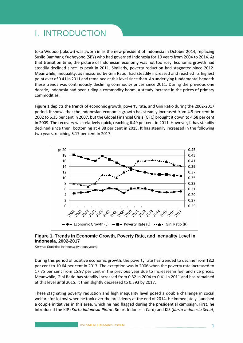
I. INTRODUCTION Joko Widodo (Jokowi) was sworn in as the new president of Indonesia in October 2014, replacing Susilo Bambang Yudhoyono (SBY) who had governed Indonesia for 10 years from 2004 to 2014. At that transition time, the picture of Indonesian economy was not too rosy. Economic growth had steadily declined since its peak in 2011. Similarly, poverty reduction had stagnated since 2012. Meanwhile, inequality, as measured by Gini Ratio, had steadily increased and reached its highest point ever of 0.41 in 2011 and remained at this level since then. An underlying fundamental beneath these trends was continuously declining commodity prices since 2011. During the previous one decade, Indonesia had been riding a commodity boom, a steady increase in the prices of primary commodities. Figure 1 depicts the trends of economic growth, poverty rate, and Gini Ratio during the 2002-2017 period. It shows that the Indonesian economic growth has steadily increased from 4.5 per cent in 2002 to 6.35 per cent in 2007, but the Global Financial Crisis (GFC) brought it down to 4.58 per cent in 2009. The recovery was relatively quick, reaching 6.49 per cent in 2011. However, it has steadily declined since then, bottoming at 4.88 per cent in 2015. It has steadily increased in the following two years, reaching 5.17 per cent in 2017.

Figure 1. Trends in Economic Growth, Poverty Rate, and Inequality Level in Indonesia, 2002-2017

Source: Statistics Indonesia (various years)

During this period of positive economic growth, the poverty rate has trended to decline from 18.2 per cent to 10.64 per cent in 2017. The exception was in 2006 when the poverty rate increased to 17.75 per cent from 15.97 per cent in the previous year due to increases in fuel and rice prices. Meanwhile, Gini Ratio has steadily increased from 0.32 in 2004 to 0.41 in 2011 and has remained at this level until 2015. It then slightly decreased to 0.393 by 2017. These stagnating poverty reduction and high inequality level posed a double challenge in social welfare for Jokowi when he took over the presidency at the end of 2014. He immediately launched a couple initiatives in this area, which he had flagged during the presidential campaign. First, he introduced the KIP (Kartu Indonesia Pintar, Smart Indonesia Card) and KIS (Kartu Indonesia Sehat,

0.25

0.27

0.29

0.31

0.33

0.35

0.37

0.39

0.41

0.43

0.45

0

2

4

6

8

10

12

14

16

18

20%

Economic Growth (L) Poverty Rate (L) Gini Ratio (R)


Indonesia Health Card), two major social assistance programmes in the area of education and health respectively. Second, he started the disbursement of village fund, which is mandated by the Law No. 6/2014 on Village, replacing the PNPM (Program Nasional Pemberdayaan Masyarakat, National Community Empowerment Programme). Other initiatives were introduced later, including the expansion of PKH (Program Keluarga Harapan, Family of Hope Programme), the Indonesian version of conditional cash transfer programme. This study aims to assess the impact of these initiatives on the efforts to increase social welfare, in particular on reducing poverty and inequality. The approach employed is following Dollar and Kraay (2002) seminal paper, which assesses the correlation of economic growth with the income growth of the poor. In this study, we correlate the real economic growth with real consumption growth of each quintile of per capita household consumption for three periods: 2004-2009, 2009-2014, and 2014-2017. The first two periods refer to the first and second Yudhoyono governments and last period refer to the first three years of Jokowi presidency. The objective is to examine whether economic growth has become more pro poor or not during the Jokowi period compared to the previous periods. The main finding of Dollar and Kraay (2002) is that the average of poorest fifth incomes rise with average incomes equiproportionally. Using several specifications, they found that the coefficient of average incomes ranges from 0.9 to 1.3 and most of it is 1. It means that each one per cent increase of average income will increase average income of the poorest fifth by also one per cent. They conclude that growth of average incomes does benefit the poor and, hence, growth is good for the poor. Dollar, Kleineberg, and Kraay (2015) extended their work using data from 151 countries for the period between 1967 and 2011. Their results still lead to the same conclusion that growth is good for the poor. In the Indonesian context, Balisacan et al. (2003) show the correlation between growth and poverty. They estimate log of average per capita consumption (instead of GDP per capita) to the log of consumption of the poor. The elasticity is about 0.7 for period 1993 to 1999. Meanwhile, Miranti (2010) examines the elasticity of growth to poverty for three periods of development. The first period is called as liberalisation (1984 - 1990), the second period is called as slower liberalisation (1990 - 1996), and the third period is recovery from the Asian financial crisis (1999 - 2002). The results from that study show that growth was pro-poor in those periods. Meanwhile, Miranti (2014) re-estimate that model for decentralization period. The results show that in the decentralization era, elasticity of average consumption to poverty is greater, but rising inequality has reduced the impact of economic growth on poverty reduction. Timmer (2004) compares Indonesia’s pro-poor growth process to regional countries and concludes that Indonesia’s growth has always benefited the poor. Although during 1967-2002 period Indonesia has experienced both weak and strong pro-poor growth, during the whole period Indonesia recorded one of the best poverty reduction in Asia. The results from Timmer (2004) suggest that persistent pro-poor growth requires simultaneous and balanced interaction between growth and distribution process. Kraay (2006) identify three potential sources of pro-poor growth: first, a higher growth of average incomes; second, higher sensitivity of poverty to growth in average incomes; and third, a poverty-reducing pattern of growth in relative incomes. Using decomposition method, the study finds the first source as the dominant factor. Hence, he suggests countries to focus on the policies and institution that drive average income growth.


II. JOKOWI’S INITIATIVES ON SOCIAL POLICY Jokowi’s direct initiatives on improving social welfare consist of two broad categories. First, expanding the coverage of social assistance programmes and making them more effective. Second, rolling out and continuously enlarging the village fund, a grant for villages mandated by Law No. 6/2014 on Village. The remaining of this section discusses each initiative in turn.

2.1 Social Assistance through Cards During the 2014 presidential campaign, Jokowi often flagged two cards – KIP (Kartu Indonesia Pintar, Smart Indonesia Card) and KIS (Kartu Indonesia Sehat, Indonesia Health Card) – as his main tools to assist the poor on accessing education and health services. The introduction of these cards followed the successful implementation of similar cards at regional levels when Jokowi became the Mayor of Surakarta in Central Java and later Governor of Jakarta. Since social protection programmes in the areas of education and health were already in operation since the late 1990s as part of the JPS (Jaring Pengaman Sosial, Social Safety Net) programme, which was launched as an effort to alleviate the social impact of the Asian Financial Crisis (AFC) that hit Indonesia during 1997-1998, the implementation of these initiatives is integrated with the existing programme. KIP was integrated with the BSM (Bantuan Siswa Miskin, Assistance for Poor Students) programme, a scholarship programme for students from poor families. In 2014, the programme provides scholarships of Rp 450,000 per year for a primary school student, Rp 750,000 per year for a junior high school student, and Rp 1,000,000 per year for a senior high school student, covering a total of 11.2 million students. The Jokowi government has increased the coverage of the KIP programme to 19.7 million students by 2016. Meanwhile, KIS was integrated with the PBI (Penerima Bantuan Iuran, Premium Assistance Recipients) programme of the JKN (Jaminan Kesehatan Nasional, National Health Insurance) programme. This programme is part of the SJSN (Sistem Jaminan Sosial Nasional, National Social Security System), which is mandated by Law No. 40/2004 on SJSN. The law requires that the JKN premium of the poor is paid for by the government through the PBI programme. In July 2013, the premium assistance is Rp19,225 per PBI recipient and the total number of recipients is 86.4 million people. In 2017, the premium assistance is Rp23,000 per recipient and the total number of participants of the KIS programme is 92.4 million people. Actually, the second Yudhoyono government introduced a card for social assistance recipients, which is called the KPS (Kartu Perlindungan Sosial, Social Protection Card) in 2013. The holder of this card is entitled to receive the benefit of the Rastra (Beras untuk Keluarga Sejahtera, Rice for Prosperous Families) programme, which is a heavily subsidized rice price programme. In addition, a KPS holder is entitled to receive the benefit of BLSM (Bantuan Langsung Sementara Masyarakat, Community Temporary Direct Assistance) programme, an unconditional cash transfer programme which is usually invoked if there is a shock to the community, such an increase in fuel prices. The Jokowi government changed the KPS card into another card called KKS (Kartu Keluarga Sejahtera, Prosperous Family Card), which continues to give its holder entitlement to receive the benefit of the Rastra programme. The number of Rastra recipients is 8.6 million households in 2004 and has almost doubled to 15.8 million households in 2017.


Meanwhile for the BLSM recipients, the Jokowi government introduced a new card called KSKS (Kartu Simpanan Keluarga Sejahtera, Prosperous Family Saving Card). The last BLSM during the Yudhoyono government was in 2013, providing a benefit of Rp 600.000 in two phases with the number of recipients being 15.5 million households. Meanwhile, the Jokowi government implemented the BLSM programme in 2014 for 6 months with the number of recipients of 15.8 million households, each household receive Rp 1,000,000 in three phases. One social assistance programme that did not experience much change in term of its design in the PKH (Program Keluarga Harapan, Family of Hope Programme), which is a conditional cash transfer programme. In fact, the Jokowi government has continuously increased the coverage of this programme, indicating the priority put by the government on PKH as the main mechanism to address poverty and inequality problem in the country. In 2014, PKH covers 2.8 million households, which was then increased to 3.5 million households in 2015, 5.9 million households in 2016, and 6 million households in 2017. Furthermore, the coverage of PKH is planned to be increased to 10 million households in 2018. The benefit received by each household recipient varies in accordance with household structure. It ranges from Rp 800,000 to Rp 3,700,000 per year per household in 2016. In 2017, the benefit received by each household switch to be single benefit of Rp1,890,000. Table 1 shows the coverage, while Table 2 shows the budget of the major social assistance programmes during 2014-2018. Table 1 indicates that from 2014 to 2018 there has been an increasing number of beneficiaries that are covered by social protection programme. The number of KIP beneficiaries were almost doubled from around 11 to 21 million students between 2014 and 2015. The number of KIS beneficiaries were increased from around 88 to 92 million people between 2015 and 2016. However, the programme that has been continuously increased very significantly is PKH, starting from just 2.8 million beneficiary households in 2014 to reach 10 million beneficiary households in 2018.

Table 1. Number of Beneficiaries of the Major Social Assistance Programmes,

2014-2018 (million)

Programme 2014 2015 2016 2017 2018

KIP/BSM2 11.1 20.95 19.68 19.71 19.7

KIS/PBI2 86.4 88.2 92.4 92.4 92.4

Rastra1 15.5 15.5 15.5 15.8 15.6

KSKS/BLSM1 15.5 15.8 - - -

PKH1 2.8 3.5 5.9 6 10

Source: World Bank (2017), Bappenas (2017)

Note: 1Household, 2Individual/student

Inline with the increase in the number of beneficiaries, Table 2 shows that the budget of major social assistance programmes has also significantly increased during the 2014-2018 period. Again PKH has experienced the largest increase with its budget more than tripled from around Rp 5.5 trillion in 2014 to Rp 17.3 trillion in 2018.


Table 2. Budget of the Major Social Assistance Programmes, 2014-2018 (Rp trillion)

Programme 2014 2015 2016 2017 2018

KIP/BSM 6.6 6.4 10.6 11.7 10.5

KIS/PBI 19.9 19.9 24.8 25.5 25.5

Rastra 18.2 21.8 22.1 19.8 21

KSKS/BLSM 6.2 9.4 - - -

PKH 5.5 6.5 7.8 11.3 17.3

Source: World Bank (2017), Bappenas (2017)

The targeting of social assistance programmes in Indonesia has evolved a long way since the social safety net (JPS) programmes of the late 1990s. Currently the application of a uniform targeting mechanism, through a national registry of around 26 million poor and vulnerable households (the Unified Database, or UDB), has improved the targeting of social assistance benefits towards the poor and vulnerable (World Bank, 2017). McCarthy and Sumarto (2018) are skeptical with the top-down approaches in targeting of the social assistance programmes. They suggest that community-based targeting, developed based on existing community practices, will produce better and more acceptable results. Actually, in recent years innovations by including community consultation (musyawarah desa or Musdes) and self-targeting (Mekanisme Pendaftaran Mandiri or MPM) have been piloted and adopted.

2.2 Village Development through Grants In addition to social assistance to households, the government also provides block grant to villages, the dana desa (village fund), as mandated by the Law No. 6/2014 on Village. These grants to villages replaced the grants to communities under the PNPM (Program Nasional Pemberdayaan Masyarakat, National Community Empowerment Programme), which was implemented from 2007 to 2014. Although the law was signed by the then President Yudhoyono nearing the end of his second term, it was only started to be implemented in 2015 when Jokowi has been inaugurated as the new president. During the 2014 presidential campaign, Jokowi already made a promise to provide a grant of Rp 1 billion to each village every year. Table 3 recapitulates the distribution of village fund from 2015 to 2018. In 2015, the government started to disburse the village fund with the average amount of Rp 280 million for each village. The average amount was continuously increased in subsequent years, reaching Rp 800 million per village in 2018. As a consequence, the total village fund distributed has tripled in just four years from around Rp 20 trillion in 2015 to reach Rp 60 trillion by 2018.

Table 3. The Distribution of Village Fund, 2015-2018

Year Average Fund per Village (Rp million)

Number of Villages

Total Village Fund (Rp trillion)

2015 280 74,754 20.8

2016 628 74,754 46.9

2017 776 74,954 58.2

2018 800 74,954 60.0

Source: Ministry of Finance (various years)


The use of village fund in each village is determined through a village planning meeting called Musrenbangdes (Musyawarah Perencanaan Pembangunan Desa, Village Development Plan Consultation), with the results formally formulated in a village budget called APBDes (Anggaran Pendapatan dan Belanja Desa, Village Income and Expenditure Budget). Most villages allocate the largest part, more than 70 per cent, of village fund for infrastructure development, in particular village roads. Only a small part of village fund is allocated for community empowerment (Syukri et al. 2018).

III. MODEL AND DATA To assess the impact of Jokowi’s social welfare initiatives on poverty and inequality, we examine whether economic growth has become more or less pro-poor during Jokowi’s period compared to the previous periods. A framework that can be used for this purpose is the model estimated by Dollar and Kraay (2002), where they correlate economic growth with income growth of the poorest quintile. While Dollar and Kraay (2002) estimate the model in a multi-country setting, we adopt the model for Indonesia using district level data. We use consumption instead of income and do some extensions where we estimate not only the elasticity of the poorest quintile (Q1), but also the middle (Q2, Q3, and Q4) and the richest (Q5) quintiles of per capita household consumption. The expectation is that Jokowi’s social welfare initiatives, which are targeted towards the poor to assist them meeting their needs, will boost the consumption growth of the poor. However, the framework used here cannot assess the impact of social welfare policies on consumption growth in isolation from other social and economic policies in place as well as shocks that occur in the economy. Therefore, the results of the analysis will show the net effect of all policies and shocks that take place in the economy on household consumption growth.

3.1 Model of Economic Growth and Consumption Growth of the Poor

Following Dollar and Kraay (2002), the model is formulated as:

𝑦𝑑𝑡𝑞= 𝛼0 + 𝛼1𝑌𝑑𝑡 + 𝛼2𝑋𝑑𝑡 + 𝜇𝑑 + 𝜀𝑑𝑡 (1)

where q, d, and t refer to quintile, district, and years respectively. 𝑦𝑑𝑡𝑞

is the logarithm of mean per

capita consumption of quintile q in district d at time t, 𝑌𝑑𝑡 is the logarithm of GDP per capita in district d at time t, and 𝑋𝑑𝑡 is a vector of control variables in district d at time t. Meanwhile, 𝜇𝑑 and 𝜀𝑑𝑡 are the cross-section district heterogeneity and time series error terms respectively. The coefficient of interest is 𝛼1 that shows the elasticity of the impact of average income toward per capita consumption of household in each quintile. Since we use the same source of data of the left and right hand side variables, which is Statistics Indonesia (BPS), there is no problem of inconsistent definition and measurement of variables, which often plague multi-country studies. To ensure robustness of our estimation, we estimate the model using several regression techniques.


First, as the basic estimation, we estimate the model using Ordinary Least Squares (OLS) technique. However, this estimation suffers from reverse causality problem and unobserved variables, resulting in downward bias of the estimates. Second, to control for unobserved heterogeneity, we run a panel fixed-effect estimation, bearing in mind that the reverse causality problem still remains. Third, to solve the reverse causality and unobserved heterogeneity problems, we use first difference estimation technique. To do this, the model in equation (1) is modified into:

𝑦𝑑𝑡𝑞− 𝑦𝑑𝑡−1

𝑞= 𝛼1(𝑌𝑑𝑡 − 𝑌𝑑𝑡−1) + 𝛼2(𝑋𝑑𝑡 − 𝑋𝑑𝑡−1) + (𝜀𝑑𝑡 − 𝜀𝑑𝑡−1) (2)

However, a new problem in the form of autocorrelation appears. Hence, fourth, in line with Dollar and Kraay (2002), we combine equations (1) and (2) into a system equation and use GMM-system estimation technique to estimate the model. However, we now have an over identification and still have the serial correlation problem. Hence, we use the Hansen test for over-identification and Arrelano-Bond’s second order test for serial correlation. Finally, fifth, to overcome the over identification and serial correlation problems, we include year and island dummy variables in the GMM-system estimation. Since we estimate the model using data from relatively short periods of time following the presidential periods, this fits with the GMM-system estimation technique that supports estimation of panel data with many individuals but few time periods (large N and small T panel data).

3.2 Data The unit of observation of the data used in the analysis is district (Kabupaten and Kota). The data consists of district per capita economic growth, district average of real per capita household consumption growth by quintile (constant 2000 price), and several district level control variables. The district economic growth is calculated from the data of district level Gross Regional Domestic Product (GRDP) constant 2000 price. Meanwhile, the per capita household consumption is calculated from the data collected through the National Socio-Economic Survey (Susenas), a household survey covering basic demographic and detailed household consumption variables. However, since Susenas is not a household panel data, the quintiles can consist of different households over time. We use the district Consumer Price Index (CPI) to deflate the nominal household consumption to obtain the real consumption data using constant 2000 price. Since the district per capita economic growth is calculated in annual term, we transform the monthly household per capita consumption into also annual value. The source of all this data is Statistics Indonesia (BPS). Between 2004 and 2017, many districts in Indonesia split. Hence, we re-aggregate the divided districts into their original districts in 2004. Our final data includes a balance panel of 377 districts, covering the period of 2004-2017. In accordance with the objective of this study, we estimate the model using data from three periods in accordance with presidential periods: 2004-2009 (SBY1), 2009-2014 (SBY2), and 2014-2017 (JKW).


IV. EMPIRICAL ESTIMATION AND DISCUSSION

4.1 Growth Incidence Curve To explore what happened to household consumption during the three periods of analysis, Figure A1 in the Appendix shows the growth incidence curve (GIC) of per capita household consumption in each period. GIC is measured as the annual growth of per capita household consumption. GIC shows the rate of pro-poor growth (Ravallion and Chen, 2003). Several observations can be made from the GIC curves. First, growth of per capita household consumption for all segments of population in all periods is always positive, implying that in general the welfare of Indonesian people has continuously increased. Second, however, the mean of the growth of per capita household consumption has declined from one period to another, implying that the pace of welfare improvement has declined over time. Third, during the first two periods, the GIC curves are positively sloped, implying that the growth of consumption is higher the richer the population. This is the underlying cause of increasing inequality observed during the period. Fourth, during the Jokowi period the form of GIC curve is inverse U-shaped, implying that the welfare improvement for the middle class is higher than for the poorest and richest population groups. This explains why inequality has slightly declined during the last two years.

4.2 Is growth good for the poor in Indonesia? The results of our estimations using various estimation techniques are shown in Table A1 to Table A5 in the Appendix. Table A1 shows the estimation results using OLS, Table A2 using fixed effect, Table A3 using first differences, Table A4 using GMM-system with the log GDP per capita instrumented using second lag of the independent variables, and Table A5 using GMM-system with control for year and region dummies. Different from Table A4, the estimation results in Table A5 pass the Hansen test for over-identification and Arellano-Bond test for serial correlation. Hence, we use these results as the main results of our analysis. We present the coefficients of log per capita GDP in Table A5 as a graph in Figure 2. Since the estimations have controlled for region and year dummies, the results obtained have taken into account both regional characteristics that do not vary over time as well as specific time shocks that affect all regions nationally. This means that, in addition to district specific controls, the results have also controlled for global level variables, such as changes in commodity prices, and national level variables, such as the decline in tax collection effort by the national government.


Figure 2. Elasticities of Per Capita Consumption Growth to Per Capita GDP Growth

The figure shows that during SBY1 and SBY2 periods, the elasticities of per capita consumption growth of the poorest 20 per cent to per capita GDP growth are close to 1, replicating the results obtained by Dollar and Kraay (2002). During SBY1 period, the elasticities of the middle quintiles are slightly less than 1. During SBY2 period, the elasticities of Q2 and Q3 quintiles are significantly lower at around 0.5, while that of Q4 quintile is 1. However, in both periods the elasticities of the richest 20 per cent are significantly higher at 1.2. This means that while growth was good for the poor, growth benefited the richest population even more. During Jokowi period, unfortunately, elasticity of the poorest 20 per cent is significantly less than 1 at 0.7. Furthermore, the higher the quintile of per capita household consumption the higher the elasticity. The richest 20 per cent, meanwhile, maintain their elasticity at around 1.2. This means that for every 1 per cent per capita GDP growth, per capita consumption of the poorest 20 per cent grows by 0.7 per cent, while that of the richest 20 per cent grows by 1.2 per cent. Hence, compared to the previous periods, growth is less good for the poor, while it is better for the middle class and even more for the richest. Manning and Pratomo (2018) find that real wages have increased significantly in recent years. Wages data in the national labour force survey (Sakernas), which they used in their analysis, refers to formal sector wages. Since formal sector workers are most likely to be located in the middle quintiles in the household per capita expenditure distribution, their finding is consistent with Figure 2 which shows significant increases in the elasticities of the middle quintiles during Jokowi’s period.

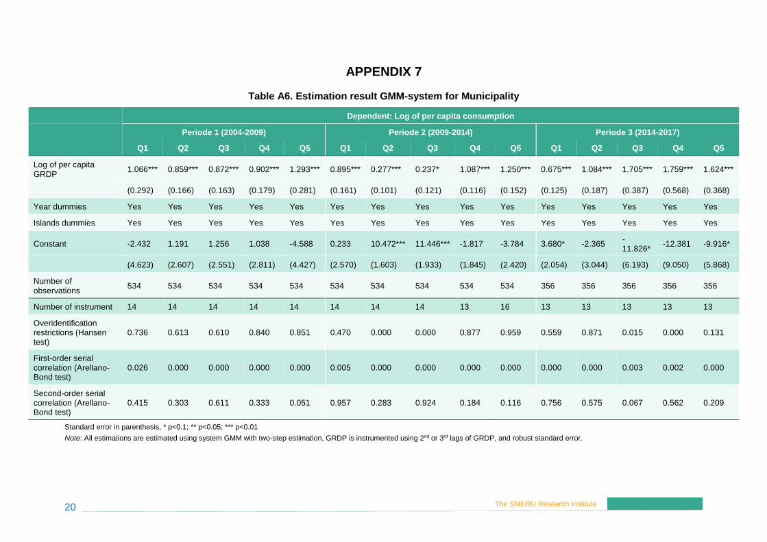
4.3 Heterogeneity Analysis To see whether the decline in the elasticity of per capita consumption growth of the poorest 20 per cent to per capita GDP growth during Jokowi period occurs uniformly across Indonesia, we perform two heterogeneity analyses. First, we split the sample into municipality districts (Kota) and regency districts (Kabupaten) and re-estimate the model separately. The results are presented in Tables A6 and A7 respectively. They show that the elasticity for the poorest 20 per cent in municipality districts is significantly lower at less than 0.7, while in regency districts it is still relatively close to one at 0.9.

0

0.2

0.4

0.6

0.8

1

1.2

1.4

2004-2009 2009-2014 2014-2017

Q1 Q2 Q3 Q4 Q5


Second, we split the sample into districts in Java island and those outside Java and again re-estimate the model separately. The results are presented in Tables A8 and A9 respectively. They show that the elasticity for the poorest 20 per cent in the districts in Java is significantly lower at around 0.7, while in the districts outside Java the elasticity is still around one. These results are actually consistent with the development priority of Jokowi, which is summarized in a motto “Membangun dari pringgiran” (developing from the periphery). However, considering that more than 60 per cent of the poor live in Java, these results imply that it is important to put more attention to assist the livelihood of the poor who live in Java and the urban poor.

V. CONCLUSION When Jokowi took over the Indonesian presidency at the end of 2014, the economic and social conditions of the country were not favourable as economic growth had been declining, while poverty reduction has stagnated and inequality was high. He has since launched several social policy initiatives to improve the welfare of the nation’s poor and vulnerable. These include expanding the coverage of several social assistance programmes as well as making them more effective. In addition, he started and continuously increases the village fund, a grant for villages mandated by the 2014 village law. This paper analyses the impact of these initiatives on poverty and inequality trends in the country. Adopting the framework developed by Dollar and Kraay (2002), we correlate economic growth with real per capita household consumption growth by quintile at the district level for three periods: 2004-2009, 2009-2014, and 2014-2017. The last period refers to the Jokowi’s period, while the first two periods refer to the first and second Yudhoyono governments. The objective is to assess whether economic growth has become more or less pro-poor under Jokowi. The results of the analysis indicate that economic growth has become less pro-poor during the first three years of Jokowi government. Compared to the ten years of SBY government, where the elasticity of per capita consumption growth to per capita GDP growth of the poorest 20 per cent population was stable at around one, during the Jokowi period the elasticity has decreased to around 0.7. This means that for every one per cent economic growth, real consumption of the poor grows less at 0.7 per cent. The clear winner of the Jokowi period is the middle class. Growth elasticities of consumption of the middle quintiles (Q2 – Q4) have increased significantly, especially compared to the second SBY period. Meanwhile, the richest 20 per cent maintains their high elasticity at around 1.2. This high level of elasticity has been consistently enjoyed by the richest population since the first SBY period. These results clearly indicate that, during the first three years of Jokowi period, the poor are less connected to economic growth compared to the middle class and the rich. This implies that Jokowi’s strategy to assist the poor through the expansion of social assistance programmes and village fund is not sufficient. While this strategy has helped the poor to maintain a positive real consumption growth, it does not really propel the poor to rise above subsistence level. Hence, a complementary strategy to connect the poor to economic growth through job creation and income generation is needed. Furthermore, the results of heterogeneity analyses indicate it is important to put more attention to assist the livelihood of the poor who live in Java and the urban poor.


LIST OF REFERENCES Balisacan, Arsenio M., Ernesto M. Pernia and Abuzar Asra. “Revisiting Growth and Poverty

Reduction in Indonesia: What do Subnational Data Show?”. Bulletin of Indonesian Economic Studies, Vol. 39, no. 3. (2003): 329-351.

Bappenas. Social Assistance Table. Jakarta: Kementerian Perencanaan Pembangunan Nasional

Republik Indonesia, Internal Documentation, 2017. Dollar, David, Tatjana Kleineberg and Aart Kraay. “Growth is Still Good for the Poor”. European

Economic Review, Vol. 81 (2015): 68-85. Dollar, David and Aart Kraay. “Growth is Good for the Poor”. Journal of Economic Growth, Vol. 7,

no. 3 (2002): 195–225. Kraay, Aart. “When is Growth Pro-Poor? Evidence from a Panel of Countries”. Journal of

Development Economics, Vol. 80, Issue 1 (2006): 198-227. Manning, Chris and Devanto Pratomo. “Labour Developments in the Jokowi Years”. Journal of

Southeast Asian Economies, this volume. (2018). McCarthy, J. and Sumarto, M. “Social Protection Program in Indonesia: Understanding the Politics

of Distribution”. Journal of Southeast Asian Economies, this volume. (2018). Ministry of Finance. Peraturan Menteri Keuangan tentang Rincian Dana Desa [Minister of Finance

Regulation on Village Fund]. Jakarta: Kementerian Keuangan Republik Indonesia, various years.

Miranti, Riyana. “Poverty in Indonesia 1984 – 2002: The impact of growth and changes in

inequality”. Bulletin of Indonesian Economic Studies, Vol. 46, no. 1 (2010): 79-97. Miranti, Riyana, Alan Duncan and Rebecca Cassells. “Revisiting the impact of consumption growth

and inequality on poverty in Indonesia during decentralisation”. Bulletin of Indonesian Economic Studies, Vol. 50, no. 3 (2014): 461-482.

Ravallion, Martin and Shaohua Chen. “Measuring pro-poor growth”. Economics Letters, Vol. 78, no.

1 (2003): 93–99. Statistics Indonesia. Statistical Yearbook of Indonesia. Jakarta: Statistics Indonesia, various years. Syukri, Muhammad, Palmira Permata Bachtiar, Asep Kurniawan, Gema Satria Mayang Sedyadi,

Kartawijaya, Rendy Adriyan Diningrat and Ulfah Alifia. Studi implementasi Undang-Undang No. 6 tahun 2014 tentang Desa: Laporan baseline [A study of the implementation of the Law No. 6/2014 on Village: A baseline report], Laporan Penelitian SMERU, Jakarta: The SMERU Research Institute, 2018.

Timmer, C. Peter. “The road to pro-poor growth: The Indonesian experience in regional

perspective”. Bulletin of Indonesian Economic Studies, Vol. 40, no. 2 (2004): 177-207.


World Bank. Indonesia Social Assistance Public Expenditure Review Update: Towards a Comprehensive, Integrated, and Effective Social Assistance System in Indonesia. Washington, D.C.: World Bank, 2017.


APPENDICES


APPENDIX 1 Figure A1. Growth Incidence Curve (GIC) of Household per Capita Consumption

Figure A1. Growth Incidence Curve (GIC) of Household per Capita Consumption

Source: SUSENAS, authors’ estimation


APPENDIX 2

Table A1. Estimation Result from OLS

Dependent: Log of per capita consumption

Period 1 (2004 -2009) Period 2 (2009 -2014) Period 3 (2014 -2017)

Q1 Q2 Q3 Q4 Q5 Q1 Q2 Q3 Q4 Q5 Q1 Q2 Q3 Q4 Q5

Log of per capita GRDP

0.252*** 0.276*** 0.288*** 0.301*** 0.308*** 0.245*** 0.274*** 0.295*** 0.314*** 0.331*** 0.250*** 0.282*** 0.305*** 0.313*** 0.314***

(0.034) (0.031) (0.029) (0.028) (0.029) (0.028) (0.027) (0.028) (0.030) (0.032) (0.026) (0.027) (0.031) (0.035) (0.042)

Constant 9.840*** 9.807*** 9.841*** 9.884*** 10.326*** 10.117*** 9.988*** 9.911*** 9.905*** 10.279*** 10.120*** 9.960*** 9.889*** 10.088*** 10.742***

(0.535) (0.488) (0.459) (0.440) (0.450) (0.441) (0.429) (0.448) (0.476) (0.505) (0.411) (0.432) (0.491) (0.566) (0.673)

Number of observations

2,262 2,262 2,262 2,262 2,262 2,262 2,262 2,262 2,262 2,262 1,508 1,508 1,508 1,508 1,508

Adjusted R2 0.345 0.376 0.389 0.391 0.322 0.369 0.400 0.403 0.398 0.352 0.358 0.385 0.399 0.393 0.366

Standard error in parenthesis, * p<0.1; ** p<0.05; *** p<0.01


APPENDIX 3

Table A2. Estimation Result from Fixed-effect





0.633*** 0.721*** 0.702*** 0.662*** 0.584*** 0.270*** 0.294*** 0.444*** 0.685*** 1.103*** 0.677*** 0.971*** 1.160*** 1.217*** 0.848***

(0.077) (0.082) (0.073) (0.069) (0.063) (0.089) (0.088) (0.102) (0.127) (0.174) (0.067) (0.100) (0.113) (0.123) (0.113)

Constant 3.898*** 2.881** 3.403*** 4.271*** 6.039*** 9.720*** 9.677*** 7.560*** 4.070* -1.879 3.320*** -1.002 -3.714** -4.308** 2.235

(1.199) (1.284) (1.129) (1.074) (0.984) (1.397) (1.385) (1.602) (2.002) (2.740) (1.063) (1.592) (1.795) (1.951) (1.793)


2,262 2,262 2,262 2,262 2,262 2,262 2,262 2,262 2,262 2,262 1,508 1,508 1,508 1,508 1,508

Adjusted R2 0.304 0.336 0.322 0.287 0.132 0.066 0.079 0.136 0.212 0.254 0.229 0.352 0.387 0.380 0.182



APPENDIX 4

Table A3. Estimation Result from First-difference





0.317*** 0.248*** 0.182*** 0.120** -0.065 0.292*** 0.012 0.052 0.210** 0.396*** 0.525*** 0.758*** 0.996*** 1.134*** 0.981***

(0.035) (0.049) (0.047) (0.049) (0.093) (0.056) (0.051) (0.051) (0.077) (0.090) (0.062) (0.089) (0.116) (0.142) (0.124)


1,885 1,885 1,885 1,885 1,885 2,262 2,262 2,262 2,262 2,262 1,508 1,508 1,508 1,508 1,508

Adjusted R2 0.068 0.040 0.022 0.008 0.000 0.033 -0.000 0.001 0.012 0.021 0.083 0.148 0.190 0.200 0.105



APPENDIX 5

Table A4. Estimation Result from GMM-system





1.054*** 0.961*** 0.901*** 0.835*** 0.484*** 0.917*** 0.304*** 0.549*** 1.016*** 1.476*** 0.889*** 1.249*** 1.584*** 1.832*** 1.358***

(0.042) (0.038) (0.037) (0.038) (0.047) (0.053) (0.042) (0.043) (0.052) (0.068) (0.047) (0.053) (0.067) (0.088) (0.133)

Constant -2.636*** -0.846 0.306 1.584*** 7.585*** -0.468 9.520*** 5.910*** -1.149 -7.755*** -0.055 -5.412*** -10.446*** -14.059*** -5.858***

(0.651) (0.584) (0.580) (0.594) (0.740) (0.832) (0.661) (0.676) (0.822) (1.068) (0.738) (0.846) (1.064) (1.402) (2.105)


2,262 2,262 2,262 2,262 2,262 2,262 2,262 2,262 2,262 2,262 1,508 1,508 1,508 1,508 1,508

Number of instrument

3 3 3 3 3 3 3 3 3 3 3 3 3 3 3

Overidentification restrictions (Hansen test)

0.176 0.290 0.297 0.388 0.180 0.687 0.108 0.584 0.802 0.506 0.200 0.015 0.001 0.000 0.000

First-order serial correlation (Arellano-Bond test)

0.000 0.000 0.000 0.000 0.000 0.000 0.000 0.000 0.000 0.000 0.000 0.000 0.000 0.000 0.000

Second-order serial correlation (Arellano-Bond test)

0.869 0.000 0.000 0.000 0.000 0.035 0.070 0.000 0.000 0.000 0.092 0.526 0.490 0.992 0.305


Note: All estimations are estimated using system GMM with two-step estimation, GRDP is instrumented using 2nd or 3rd lags of GRDP, and robust standard error.


APPENDIX 6

Table A5. Estimation Result from GMM-system with year and island dummies





0.908*** 0.844*** 0.851*** 0.907*** 1.182*** 0.964*** 0.463*** 0.521*** 1.013*** 1.240*** 0.704*** 0.850*** 1.090*** 1.166*** 1.243***

(0.089) (0.070) (0.067) (0.072) (0.102) (0.096) (0.045) (0.047) (0.047) (0.065) (0.056) (0.063) (0.099) (0.133) (0.126)

Year dummies Yes Yes Yes Yes Yes Yes Yes Yes Yes Yes Yes Yes Yes Yes Yes

Island dummies Yes Yes Yes Yes Yes Yes Yes Yes Yes Yes Yes Yes Yes Yes Yes

Constant -0.400 1.090 1.290 0.706 -3.017* -1.057 7.176*** 6.658*** -0.839 -3.686***

2.968*** 1.093 -2.310 -3.185 -3.711*

(1.391) (1.073) (1.028) (1.096) (1.543) (1.483) (0.671) (0.748) (0.720) (1.009) (0.880) (0.971) (1.516) (2.050) (1.948)


2,262 2,262 2,262 2,262 2,262 2,262 2,262 2,262 2,262 2,262 1,508 1,508 1,508 1,508 1,508


14 14 14 14 14 14 14 14 13 16 13 13 13 13 13


0.131 0.799 0.642 0.683 0.874 0.136 0.000 0.000 0.920 0.554 0.143 0.773 0.000 0.000 0.000


0.000 0.000 0.000 0.000 0.000 0.000 0.000 0.000 0.000 0.000 0.000 0.000 0.000 0.000 0.000


0.445 0.974 0.717 0.523 0.002 0.171 0.008 0.013 0.470 0.530 0.399 0.270 0.335 0.602 0.751

Standard error in parenthesis, * p<0.1; ** p<0.05; *** p<0.01 Note: All estimations are estimated using system GMM with two-step estimation, GRDP is instrumented using 2nd or 3rd lags of GRDP, and robust standard error.


APPENDIX 7

Table A6. Estimation result GMM-system for Municipality


Periode 1 (2004-2009) Periode 2 (2009-2014) Periode 3 (2014-2017)



1.066*** 0.859*** 0.872*** 0.902*** 1.293*** 0.895*** 0.277*** 0.237* 1.087*** 1.250*** 0.675*** 1.084*** 1.705*** 1.759*** 1.624***

(0.292) (0.166) (0.163) (0.179) (0.281) (0.161) (0.101) (0.121) (0.116) (0.152) (0.125) (0.187) (0.387) (0.568) (0.368)


Islands dummies Yes Yes Yes Yes Yes Yes Yes Yes Yes Yes Yes Yes Yes Yes Yes

Constant -2.432 1.191 1.256 1.038 -4.588 0.233 10.472*** 11.446*** -1.817 -3.784 3.680* -2.365 -11.826*

-12.381 -9.916*

(4.623) (2.607) (2.551) (2.811) (4.427) (2.570) (1.603) (1.933) (1.845) (2.420) (2.054) (3.044) (6.193) (9.050) (5.868)


534 534 534 534 534 534 534 534 534 534 356 356 356 356 356

Number of instrument 14 14 14 14 14 14 14 14 13 16 13 13 13 13 13


0.736 0.613 0.610 0.840 0.851 0.470 0.000 0.000 0.877 0.959 0.559 0.871 0.015 0.000 0.131


0.026 0.000 0.000 0.000 0.000 0.005 0.000 0.000 0.000 0.000 0.000 0.000 0.003 0.002 0.000


0.415 0.303 0.611 0.333 0.051 0.957 0.283 0.924 0.184 0.116 0.756 0.575 0.067 0.562 0.209




APPENDIX 8

Table A7. Estimation result GMM-system for Regency





1.157*** 0.916*** 0.869*** 0.913*** 1.323*** 1.321*** 0.276*** 0.416*** 1.018*** 1.339*** 0.909*** 0.828*** 1.159*** 1.317*** 1.485***

(0.168) (0.112) (0.097) (0.106) (0.198) (0.133) (0.067) (0.064) (0.055) (0.073) (0.056) (0.075) (0.101) (0.167) (0.182)



Constant -4.165* -0.093 0.911 0.529 -5.184* -6.553*** 9.707*** 7.926*** -1.011 -5.237*** -0.224 1.314 -3.381** -5.414** -7.325***

(2.527) (1.664) (1.451) (1.576) (2.923) (2.006) (1.034) (1.052) (0.838) (1.121) (0.873) (1.128) (1.509) (2.484) (2.722)


1,728 1,728 1,728 1,728 1,728 1,728 1,728 1,728 1,728 1,728 1,152 1,152 1,152 1,152 1,152


14 14 14 14 14 14 14 14 13 16 11 14 14 14 14


0.410 0.725 0.888 0.874 0.187 0.520 0.000 0.000 0.266 0.392 0.382 0.291 0.145 0.000 0.000


0.000 0.000 0.000 0.000 0.000 0.003 0.000 0.000 0.000 0.000 0.000 0.000 0.000 0.000 0.000


0.235 0.699 0.613 0.760 0.031 0.177 0.015 0.005 0.090 0.740 0.497 0.297 0.699 0.481 0.385




APPENDIX 9

Table A8. Estimation result GMM-system for Java





0.837*** 0.768*** 0.780*** 0.939*** 1.226*** 0.798*** 0.438*** 0.770*** 0.920*** 1.379*** 0.727*** 0.955*** 1.239*** 1.352*** 1.531***

(0.111) (0.092) (0.098) (0.128) (0.075) (0.076) (0.061) (0.062) (0.075) (0.106) (0.088) (0.116) (0.186) (0.227) (0.216)


Provincial dummies Yes Yes Yes Yes Yes Yes Yes Yes Yes Yes Yes Yes Yes Yes Yes

Constant 1.094 2.472* 2.497 0.207 -3.813*** 1.643 7.718*** 2.702*** 0.621 -5.963*** 2.700* -0.590 -4.892* -6.350* -8.513**

(1.746) (1.437) (1.539) (2.014) (1.174) (1.201) (0.961) (0.967) (1.182) (1.678) (1.404) (1.830) (2.942) (3.591) (3.426)


744 744 744 744 744 744 744 744 744 744 496 496 496 496 496


16 16 16 15 15 15 15 15 16 16 14 14 14 14 14


0.185 0.274 0.258 0.318 0.314 0.635 0.000 0.024 0.331 0.909 0.922 0.576 0.000 0.000 0.000


0.000 0.000 0.000 0.000 0.000 0.000 0.000 0.000 0.000 0.000 0.001 0.001 0.000 0.000 0.000


0.260 0.576 0.987 0.314 0.012 0.812 0.101 0.245 0.275 0.257 0.902 0.212 0.504 0.233 0.786




APPENDIX 10

Table A9. Estimation result GMM-system for Outside Java





1.250*** 1.004*** 0.977*** 1.022*** 1.305*** 1.163*** 0.437*** 0.549*** 0.966*** 1.248*** 0.955*** 0.873*** 1.176*** 1.343*** 1.408***

(0.181) (0.118) (0.111) (0.118) (0.170) (0.125) (0.066) (0.073) (0.062) (0.081) (0.063) (0.079) (0.113) (0.177) (0.171)



Constant -5.747** -1.549 -0.899 -1.348 -5.263** -4.353** 7.472*** 5.930*** -0.390 -4.219*** -1.179 0.535 -3.986** -6.326** -6.720**

(2.859) (1.851) (1.746) (1.851) (2.671) (1.968) (1.040) (1.142) (0.979) (1.272) (0.991) (1.246) (1.790) (2.786) (2.704)


1,518 1,518 1,518 1,518 1,518 1,518 1,518 1,518 1,518 1,518 1,012 1,012 1,012 1,012 1,012


12 12 12 12 12 12 12 12 11 12 10 11 11 11 11


0.398 0.728 0.720 0.679 0.568 0.508 0.000 0.000 0.008 0.059 0.405 0.106 0.113 0.000 0.000


0.000 0.000 0.000 0.000 0.000 0.007 0.000 0.000 0.000 0.000 0.000 0.000 0.000 0.000 0.000


0.631 0.684 0.721 0.827 0.021 0.175 0.056 0.050 0.193 0.986 0.744 0.751 0.732 0.049 0.796

Standard error in parenthesis, * p<0.1; ** p<0.05; *** p<0.01 Note: All estimations are estimated using system GMM with two-step estimation, GRDP is instrumented using 2nd or 3rd lags of GRDP, and robust standard error.

Telephone : +62 21 3193 6336

Fax : +62 21 3193 0850

E-mail : [email protected]

Website : www. smeru. or.id

Facebook : The SMERU Research Institute

Twitter : @SMERUInstitute

YouTube : SMERU Research Institute

Date post:	06-Jul-2019
Category:	Documents
Upload:	trinhcong
View:	214 times
Download:	0 times

Jokowi’s Initiatives to Reduce Poverty and Inequality · Jokowi’s direct initiatives on...

Documents