Regional income distribution in Mexico: new long-term evidence, 1895-2010 José Aguilar-Retureta

Col.lecció d’Economia E15/323

UB Economics Working Papers 2015/323

Regional income distribution in Mexico: new long-term evidence, 1895-2010

Abstract: In the last years, Economic History literature has paid close attention to the long-term changes undertaken by regional income inequality in different countries after the integration of their domestic markets. Nevertheless, this literature has mainly focused on developed economies (US and Europe). New evidence is required from peripheral economies, where economic growth has had different features, and income inequality may have been dominated by other forces and followed different trends. The aim of this paper is to analyse several dimensions of the long-term evolution of Mexican regional income inequality, from the early stages of domestic markets integration to the present (1895–2010). This analysis may be taken as basis for further explanatory analysis and may contribute to the emergence of new hypothesis to explain the long-term changes in regional inequality in peripheral economies. JEL Codes: N16, N96, R11. Keywords: Economic History, Regional Inequality, Economic Growth.

José Aguilar-Retureta Universitat de Barcelona

Acknowledgements: This paper is part of my PhD dissertation, carried out under the supervision of Alfonso Herranz-Loncán and Marc Badia-Miró. This research has been funded by the CONACyT scholarships for PhD studies abroad program. I also want to acknowledge the financial support received from the Institut Ramon Llull (Generalitat de Catalunya), the research project ECO2012-39169-C03-02 financed by the Spanish Ministry of Economy and Competitiveness, and the Xarxa de Referència d'R+D+I en Economia i Polítiques Públiques financed by the Catalan government. I am in debt to Alfonso Herranz-Loncán and Marc Badia-Miró for their constant support during my PhD research. I also thank the participants at the “Regional GDPs in Latin America, a long-term perspective (1870-2010)” symposium, held at the 4th Latin America Economic History Congress (Bogotá, Colombia), as well as the participants at the Second workshop “The New Economic Historians of Latin America”, at the University of Geneva, and the “PhD students’ Seminar in Economic and Social History” at the University of Oxford. I also wish to thank Alejandra Irigoin, Juan Flores, Joan Rosés, and Max-Stephan Schulze for their very useful comments on this paper.

ISSN 1136-8365

  3

1. Introduction

In the last years, the evolution of regional income distribution and its

determinants has been paid close attention in the Economic History literature.

Scholars have mainly focused on core economies, for which the available evidence

suggests that spatial inequality has commonly followed an inverted-U shape in the

long term.1 This was the consequence of a process of regional income divergence

during the first stages of domestic markets integration, and a further decrease in

disparities as economic growth and national market integration continued moving

forward.2 These findings are consistent with some of the predictions of the New

Economic Geography (NEG), and also fit with the seminal Williamson’s (1965)

‘inverted-U’ trend proposal. The NEG framework suggests that the interaction

between the fall in transport costs, increasing returns and market potential can first

lead to economic activity agglomeration, increasing therefore regional income

inequalities (Krugman, 1991). However, firms may gradually become sensitive to

congestion costs if trade costs continue falling, causing a subsequent dispersion of

the economic activity (Puga, 1999). Thus, market integration might eventually lead

to regional income convergence. On the other hand, the ‘inverted-U’ pattern

described by Williamson (1965) could be understood as an extension of the Kuznets’

curve at the regional level, implying that in the early stages of industrialization

regional inequalities within countries tend to increase, to decrease thereafter from the

moment when industrialization spreads across most regions. In both theoretical

                                                                                                               1 While several studies (e.g. Geary and Stark, 2002; Crafts and Mulatu, 2005; Rosés, Martínez-Galarraga, and Tirado, 2010; Combes, Lafourcade, Thisse, and Toutain, 2011; Felice, 2011; Henning, Enflo, and Andersson, 2011; Martínez-Galarraga, 2012; Badia-Miró, Guilera, and Lains, 2012; Martínez-Galarraga, Rosés, and Tirado, 2013; Enflo and Rosés, 2014; Geary and Stark, 2015) focus on several European countries; Kim (1998, 1999), and Klein and Crafts (2012), analyse the US case. 2 The Italian and Swedish cases are an exception to this pattern (Felice, 2011 and Enflo and Rosés, 2014, respectively).

  4

frameworks regional income inequality is determined, essentially, by the location

decisions of industrial activity.

Nevertheless, very little evidence is available on developing countries, in

which the patterns and causes of the long-term evolution of spatial economic

distribution may have been far different from those of the industrialized countries.

Actually, the analysis of peripheral economies may provide new hypothesis and

perspectives on the forces behind regional economic growth and regional inequality.

Recently, Badia-Miró (2014), has pointed out that the characteristics and

determinants of long term Chilean regional income inequality (1890–2000) do not

match those found in industrialised economies. To start with, the Chilean case does

not follows the ‘inverted-U’ pattern described above; instead, there was sustained

regional convergence in Chile over the period of the study. Moreover, the author

points out that, despite the extremely high economic activity concentration in the

Santiago region (Chile’s administrative capital), this did not result in higher income

productivity relatively to the rest of the country, suggesting that agglomeration

economies could not have been the main determinant behind Chilean’s regional

inequality trend. Similarly, Caruana-Galizia (2013) shows that Indian regional

income inequality experienced β- and σ- convergence during the first stages of

domestic market integration (1875-1911), which contrasts with the divergence

process suggested for the core economies in the same historical period.

The long-term evolution of Mexican regional inequality has not been

analysed yet from an Economic History perspective. Historians have instead focused

on particular regions and/or the regional distribution of particular sectors,3 and the

                                                                                                               3 Kuntz (2010, 2014) has widely studied the impact of the export-activity on the spatial economic performance. Likewise, Mario Cerutti has contributed to the understanding of the historical economic development in the northern states (see Cerutti, 1992). On the other hand, Haber (1989) provides a

  5

aggregate study of regional inequality, which has often been approached through β-

convergence and σ-convergence analyses, has usually been restricted to the most

recent decades (see Esquivel, 1999; Sánchez-Reaza and Rodríguez-Pose, 2002;

Chiquiar, 2005; Rodríguez-Oreggia, 2005; Carrion-i-Silvestre and German-Soto,

2007; Ruiz, 2010; Brock and Germán-Soto, 2013).4 Moreover, even though these

convergence studies are useful to understand regional inequality trends, they provide

a highly simplified view of the historical evolution of regional income distribution

process, as they totally ignore the spatial location component (Yamamoto, 2008). For

instance, convergence analyses do not take into account the possible impact that a

relatively rich region may have on the nearby areas (spatial clustering), or how the

shapes of income distribution evolve over the long run. These dimensions of regional

income disparities are highly relevant in the long run. For example, in the Mexican

case, it would be essential to understand the impact of Mexico City on its closest

states or the effect of the US on the northern states.5

In this regard, the present article aims to analyse multiple dimensions of the

Mexican regional income inequality evolution in the long term, since the period in

which domestic markets got integrated to nowadays (1895–2010). Firstly, I present

some conventional indicators of regional inequality, such as the Coefficient of

Variation (CV), the Gini coefficient, and the Theil, Williamson and Herfindahl-

Hirschman indexes. Secondly, I estimate Kernel distributions of regional income, in

order to provide a picture of the shape and modality of spatial income distribution in

                                                                                                                                                                                                                                                                                                                         detailed description of the industrialisation process during the primary-export model, from 1890 to 1930. 4 This literature has been concentrated, due to the lack of a GDP per capita database at state level, on the decades after 1940 and, specially, the period after the opening of the economy since the middle of the 1980s. 5 These two facts have been pointed out as one of the most important causes of the regional economic growth in Mexico both during the ISI period and the subsequent stage of economic openness, especially since the North America Free Trade Agreement (NAFTA) came into effect in 1994 (Jordaan and Sanchez-Reaza, 2006).

  6

the long term. Thirdly, I analyse regional income mobility through the Spearman

rank and the Kendall’s τ-statistic. Last but not least, I use the Moran’s I coefficient to

study the intensity of spatial clustering of regional incomes per capita. All these

indicators aims at complementing the available evidence of the Mexican regional

income disparities over the long term, and at contributing to the international

literature on historical regional inequality, by providing evidence on an economy that

did not belong to the western core.6

The long-term perspective adopted in this paper allows a detailed analysis of

the evolution of regional income inequality across the different economic models

that have been adopted in Mexico since the start of modern economic growth. More

specifically, the period under analysis includes the agro-export model of the first

international globalisation (1895–1930), the State-Led Industrialization period

(1930–1980) and the current model of high economic openness (1980–2010). The

long-term study of Mexican spatial inequality may be of interest for economic

policy-makers, since the presence of North-South economic development

polarization is yet to be resolved. According to the National Council for Evaluation

of Social Development Policy (CONEVAL), 43 per cent of the total population

living in extreme poverty in 2010, was located in 4 Southern States: Chiapas,

Guerrero, Oaxaca and Veracruz. Moreover, in a recent publication, the ECLAC

(2014: 73) has pointed out that Mexico had, ca. 2010, the second highest income

ratio between the richest and the poorest region among Latin America countries, only

after Ecuador.

                                                                                                               6 Recent literature has applied similar techniques to explain multiple dimensions of regional per capita income disparities within different countries, see Bosch, et al. (2003), Aroca, et al. (2005), Yamamoto (2008), Germán-Soto and Escobedo (2011), Herranz-Loncán and Martínez-Galarraga (2013), Badia-Miró (2014), and Tirado and Badia-Miró (2014). Moreover, a distribution dynamics analysis among the OECD countries in the long-term can be found in Epstein et al. (2003).

  7

The article is structured as follows. Next section offers a brief summary of

the Mexican economic growth process since the late 19th century. Section 3 presents

a long-run description of Mexican regional income distribution, on the basis of

several indicators. In section 4, spatial econometrics is used to test the presence of

spatial income autocorrelation among Mexican states. Conclusions are presented in

section 5.

Map 1 Mexican administrative division

 

Source: Own elaboration, using QGIS. The map was taken from: www.divas-gis.org  

2. Regional economic growth in Mexico in the long run

The economic growth of the Mexican regions has been affected in the long-

term by the economic model adopted in each historical period. First, the primary-

export boom, that took place from the late nineteenth century to the 1929 Great

Depression, caused important changes in the country’s economic structure. The

introduction of the railways was crucial not only to enhance exports but also to

  8

integrate national markets, bringing about a boost in regional economic

specialization.7 Indeed, historians have pointed out that it was at this moment that

Mexico embraced the capitalist system (Kuntz, 2010). Besides, during this period the

country went through an important process of economic modernization, largely

associated to the expansion of industry and, specially, the mining sector. According

to Stephen Haber, “the first wave of modern Mexican industrialization” extended

from the 1890’s to the 1930’s (Haber, 1989:3), and it was largely a consequence of

export growth (Haber, 2010). During this period, both the domestic market and

national production developed, and the railroads played a crucial role in the process

of economic regional specialization (Dobado and Marrero, 2005; Kuntz, 1999).

The industrial, mining, and agro-exporter sectors were the main forces behind

the transformation of the national economic structure (Kuntz, 2010:321). Whereas

these sectors accounted for a growing share of total GDP, agriculture for domestic

consumption gradually fell behind. According to Pérez López (1960), the

participation of manufacturing and mining in total GDP grew from 9.1% to 13.2%,

and from 4.9% to 9.5% respectively between 1895 and 1929.8 Instead, the share of

agriculture within GDP decreased from 23.8% in 1895 to 13.9% in 1929. This

process of structural change is essential to understand the increase in differences

among regions throughout the period. The states in which industry and mining were

located had a much higher dynamism than the rest. As Aguilar-Retureta (2015) has

pointed out, Mexico City, the northern region, and some particular states (Veracruz

                                                                                                               7 Together with the rail expansion, the effective elimination of the alcabalas (tax on domestic commerce) in the late 1890s had a relevant impact on domestic market integration; see Kuntz (2010:315). See Dobado and Marrero (2005) for commodity market integration, and Kuntz and Speckman (2011) for labour market integration. 8 Furthermore, since the liberal reforms the mining sector undertook a process of modernization, which increased both its value added and productivity (especially from 1890, when some US companies moved its production plants to Mexico due to the US protectionist policy in this sector, together to a strong Mexican fiscal stimulus).

  9

and Yucatán) were the best performing areas during this period. Yucatán benefitted

from the most successful agro-export activity: the henequen.9 On the other hand, the

industrial activity was concentrated in Mexico City, Veracruz and the north

(specially Nuevo León). According to my estimates, the participation of these three

states in the country’s total manufacturing activity increased from 19.5% in 1895, to

46.9% in 1930. 10 By contrast, the mining sector experienced an increasing

geographic dispersion during this period (although it was also mostly concentrated in

the north and north-centre regions). This dispersion might have partially overcome

the effects of industrial concentration on regional income inequality, as happened in

the Chilean case (Badía-Miró, 2013). However, the estimates presented in Aguilar-

Retureta (2015) clearly show that both, the Mexico City economic dynamism and the

north/south division of the country, started at least in the late nineteenth century.

After the primary-export boom, Mexico undertook a process of accelerated

industrialization based on domestic markets’ growth (1930-1985). This period is

commonly known in Latin America as the Import Substitution Industrialization (ISI)

period. The main features of this model were the shift to industrialization as the

engine of economic development and a strong State intervention in the economy

(Bértola and Ocampo, 2010:151). The ISI period is generally considered as a closed-

economy model, due to the strong commercial protectionist strategy adopted in those

years. It was during this period when the Mexican economy experienced the greatest

growth rates since the consolidation of domestic markets, having an annual average

GDP growth rate of 5.24% and 6.38% during the years 1932-1949 and 1949-1981                                                                                                                9 In fact, this was the only non-mining successful export commodity during the First Globalisation (Riguzzi, 1995:174). 10 Therefore, the process of manufacturing concentration in the capital and the north started at least in the last years of the 19th century. This would partially contradict some recent research, in which industrial concentration in Mexico City is assumed to have started with the ISI policies; see, for instance, Krugman and Livas (1996:140). My estimates suggest that this process began well before the ISI period, although it substantially accelerated after 1930, since in 1975 the “Capital” region accumulated 51.8% of total manufacturing production (see Hernández, 1980: 140).

  10

respectively (Márquez, 2010: 553). The low level of international integration had

strong economic implications at the regional level, and it especially encouraged the

intensification of economic concentration. Although, during this period, various

political programs attempted to de-centralize different economic activities and the

industrial sector in particular, the latter was greatly concentrated in Mexico City and

the surrounding areas (especially the State of Mexico), together with a few other

states such as Jalisco and Nuevo León.11

The concentration of industrial activity in Mexico City has been theoretically

explained on the basis of New Economic Geography’s predictions. Krugman and

Livas (1996) explain why industrial activity during this period tended to concentrate

in the largest market in the country (Mexico City). In general terms, the authors show

that this agglomeration responded, under a closed economy model, to the emergence

of strong forward and backward linkages in the biggest market, in order to supply the

goods demanded there.12 As a consequence, according to Germán-Soto (2005),

Mexico City, together with the State of Mexico, represented 36.14% of Mexico’s

total GDP in 1980. Nevertheless, despite the high concentration of economic activity

in Mexico City, the literature has also identified a reduction of regional income

disparities during this period. Following Sánchez-Reaza and Rodriguez-Pose

(2002:77), this can be explained, for the late years of the ISI period, by the oil

production boom of the 1970s and 1980s, which was mostly located in the Southeast

of Mexico, and, secondly, by the rapid out-migration from the southern sates to the

rest of the country and the US.

By the middle of the 1980s, the Mexican economy started a process of

                                                                                                               11 During the ISI period, the government tried to encourage the dispersion of industrial activity, for example, by promoting the creation of industrial parks in different states. Nevertheless, those political efforts were not successful (Aguilar, 1993:341). 12 See Hernández, E. (1980) for a narrative confirming the NGE hypothesis for the Mexican case during the ISI period.

  11

increasing openness and decreasing state intervention. The debt crisis and the

downfall of the oil price are the main factors behind the collapse of the ISI model.

The new Mexican export-promotion strategy started with the adhesion of Mexico to

the General Agreement on Tariffs and Trade (GATT) in 1986, and continued with a

deepening in regional international integration in 1994 through the signature of the

North American Free Trade Agreement (NAFTA). According to the World Bank,

Mexican openness rate was 24% in 1980 and 61% in 2010 respectively (World Bank,

2014). The process of economic openness and regional international integration has

significantly affected the patterns and trends of regional growth in Mexico during the

last twenty years, specially benefitting the north-border states. Rodríguez-Oreggia

(2005: 219) has pointed out that, in general, the regions that were catching up in

1970-1985 (under a closed economy), lagged behind since the opening of the

economy. On the other hand, the states that were falling behind during the last years

of the ISI period (namely, some of the north border states) became the winners

afterwards. Once again, the NEG framework is useful to explain these changes.

Krugman and Livas (1996:150) describe how, after the process of economic

liberalization, there was no longer enough dependence on the domestic market

(namely, Mexico City) to make the backward and forward linkages strong enough to

support the large concentration of production in Mexico City. Thus, because of the

trade liberalization policies, the firms have increasingly found these linkages in the

international market (mainly in the US), and therefore, have tended to move closer to

this market, at the north-border regions. In 2012, the north-border states (6 out of 32)

account for 52.87% of the total exports value.13 Meanwhile, Mexico City and the

State of Mexico, for instance, only represent 6.3% of national exports (INEGI,

                                                                                                               13 77.6% of total exports were destined to the US in the same year.

  12

2014).14 Hanson (1998a, 1998b) has observed the same trend in manufacturing

employment: free trade in North America has boosted, on the one hand, the

expansion of manufacturing labour force in the north-border states and, on the other

hand, the contraction of this sector in Mexico City.

Following this historical review, the next section presents several measures of

Mexican regional income disparities in the long run, beyond the well-known β-

convergence and σ-convergence analyses that have been the object of most previous

literature.

3. The long-run trends of regional income disparities in Mexico, 1895-2010

In order to present the trends and patterns of regional income inequalities in

Mexico since the late nineteenth, I use the GDP per capita estimated by Aguilar-

Retureta (2015). Table 1 shows these figures, in benchmark years from the early 20th

century to the present. As it can be noted, there is a marked persistence of the high pc

GDP levels of both Mexico City and the North region and, on the other side, a poor

income performance of the Centre and South regions in relation to the national

average over the long run. On the basis of these data, the next section presents

several indicators that allow approaching the different dimensions of the long-term

evolution of Mexican regional income disparities.

                                                                                                               14 Thanks to oil exports, Campeche and Tabasco were the origin of 13.77% of the national exports value.

  13

Table 1 Regional per capita GDP in Mexico: 1900, 1930, 1950, 1980, and 2010 (Mexico = 1)

1900 1930 1930* 1950 1950* 1980 1980* 2010 2010* Mexico City 2.61 2.71 2.83 2.63 2.71 1.91 2 2.27 2.39 North 1.71 2.21 2.27 1.59 1.64 1.19 1.25 1.22 1.27 Baja C. North 3.11 4.4 4.54 2.87 2.96 1.28 1.34 1.03 1.08 Baja C. South n.d. n.d. n.d. 1.18 1.22 1.27 1.33 1.11 1.16 Chihuahua 1.29 1.82 1.89 1.41 1.45 0.94 0.99 1.04 1.09 Coahuila 1.46 1.72 1.78 1.28 1.33 1.15 1.2 1.31 1.37 Nuevo León 1.6 1.66 1.71 1.57 1.62 1.58 1.65 1.9 1.97 Sonora 1.79 1.77 1.82 1.56 1.61 1.08 1.14 1.05 1.11 Tamaulipas 1.03 1.9 1.85 1.28 1.31 1.03 1.08 1.12 1.08 Pacific-North 1.22 0.77 0.79 0.81 0.84 0.85 0.89 0.88 0.93 Colima 0.91 0.8 0.82 0.83 0.85 0.91 0.95 1.01 1.06 Jalisco 0.98 0.55 0.57 0.71 0.74 1.01 1.06 1.01 1.06 Nayarit 1.51 0.78 0.8 0.74 0.77 0.71 0.74 0.65 0.69 Sinaloa 1.46 0.93 0.96 0.95 0.98 0.76 0.79 0.85 0.9 Centre-North 1.25 0.89 0.91 0.62 0.64 0.64 0.67 0.85 0.89 Aguascalientes 2.13 0.88 0.91 0.46 0.48 0.79 0.83 1.1 1.16 Durango 1.32 0.97 1 0.75 0.78 0.72 0.76 0.86 0.9 San Luis Potosí 0.68 0.84 0.83 0.7 0.71 0.58 0.61 0.79 0.83 Zacatecas 0.86 0.85 0.88 0.55 0.57 0.47 0.49 0.63 0.66                    Gulf of Mexico 1.14 1.03 0.97 1.1 1.06 1.18 0.82 1.72 0.96 Campeche 0.98 0.88 0.91 0.84 0.87 0.76 0.8 4.39 1.17 Tabasco 0.83 0.68 0.7 0.57 0.59 2.51 0.58 1.41 0.71 Quintana Roo n.d. n.d. n.d. 1.93 1.99 1.2 1.25 1.28 1.35 Veracruz 0.97 1.26 0.91 1.28 0.97 0.72 0.73 0.68 0.67 Yucatán 1.77 1.3 1.34 0.87 0.90 0.72 0.75 0.84 0.88 Centre 0.86 0.65 0.68 0.5 0.52 0.73 0.76 0.76 0.8 Guanajuato 0.82 0.54 0.65 0.46 0.48 0.65 0.68 0.84 0.88 Hidalgo 0.79 0.62 0.83 0.43 0.45 0.66 0.69 0.61 0.64 Morelos 1.28 0.79 0.74 0.79 0.81 0.77 0.8 0.77 0.81 Puebla 0.87 0.7 0.72 0.53 0.55 0.65 0.68 0.69 0.73 Querétaro 0.76 0.51 0.53 0.41 0.43 0.86 0.9 1.14 1.2 State of Mexico 0.64 0.68 0.56 0.51 0.53 0.97 1.02 0.72 0.76 Tlaxcala 0.84 0.72 0.7 0.37 0.38 0.55 0.58 0.53 0.55 South 0.6 0.4 0.41 0.4 0.41 0.59 0.52 0.51 0.53 Chiapas 0.74 0.5 0.52 0.4 0.42 0.87 0.5 0.44 0.44 Guerrero 0.41 0.28 0.29 0.4 0.41 0.53 0.56 0.52 0.55 Michoacán 0.77 0.49 0.51 0.42 0.44 0.55 0.58 0.63 0.66 Oaxaca 0.46 0.31 0.32 0.36 0.37 0.4 0.42 0.45 0.48 Source: Aguilar-Retureta (2015) (*) Oil production excluded.  

  14

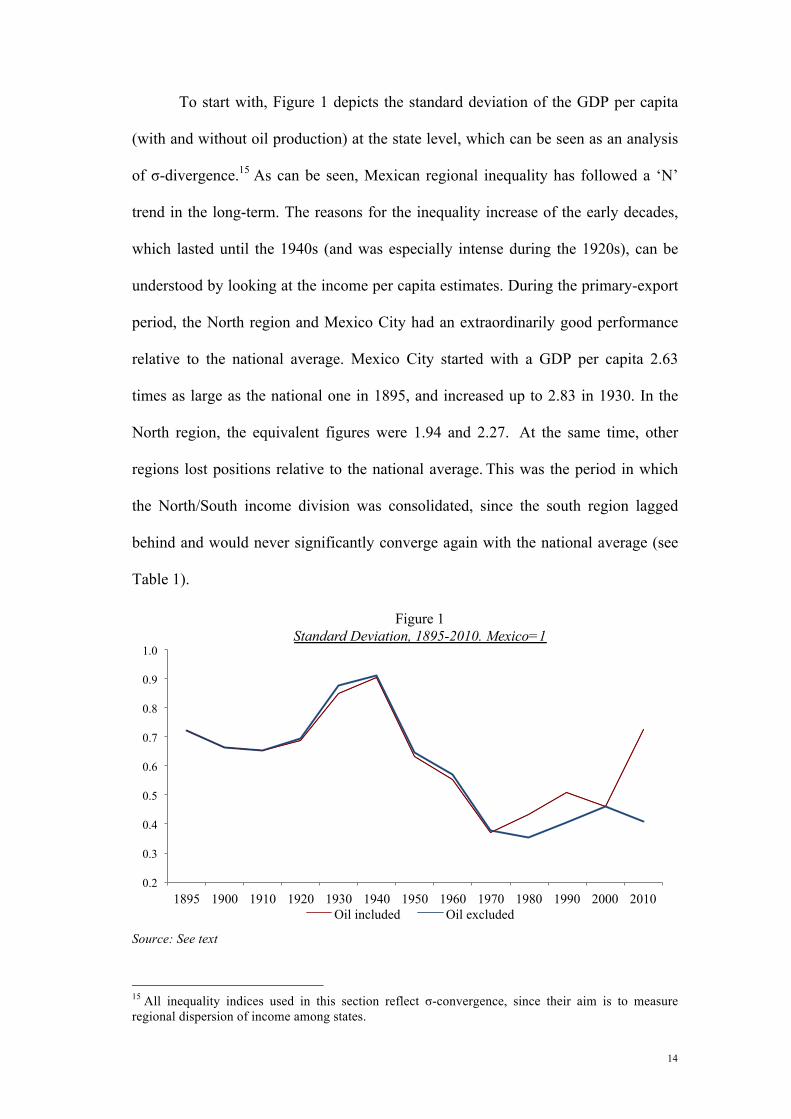
To start with, Figure 1 depicts the standard deviation of the GDP per capita

(with and without oil production) at the state level, which can be seen as an analysis

of σ-divergence.15 As can be seen, Mexican regional inequality has followed a ‘N’

trend in the long-term. The reasons for the inequality increase of the early decades,

which lasted until the 1940s (and was especially intense during the 1920s), can be

understood by looking at the income per capita estimates. During the primary-export

period, the North region and Mexico City had an extraordinarily good performance

relative to the national average. Mexico City started with a GDP per capita 2.63

times as large as the national one in 1895, and increased up to 2.83 in 1930. In the

North region, the equivalent figures were 1.94 and 2.27. At the same time, other

regions lost positions relative to the national average. This was the period in which

the North/South income division was consolidated, since the south region lagged

behind and would never significantly converge again with the national average (see

Table 1).

Source: See text

                                                                                                               15 All inequality indices used in this section reflect σ-convergence, since their aim is to measure regional dispersion of income among states.

0.2

0.3

0.4

0.5

0.6

0.7

0.8

0.9

1.0

1895 1900 1910 1920 1930 1940 1950 1960 1970 1980 1990 2000 2010

Figure 1 Standard Deviation, 1895-2010. Mexico=1

Oil included Oil excluded

  15

From the 1940s onwards, coinciding with the ISI model consolidation, an

accelerated process of regional income convergence took place. This tendency

continued until the economic liberalization of the 1980s. From then on, regional

divergence has been a constant –with the exception of the 2000s. This recent

divergence can be explained because, while the poorest states (mainly the south)

have remained far below the national average income, the north-border region has

kept its income advantage and some particular states, such as Guanajuato (Centre-

north region), Querétaro (Centre region), and Quintana Roo (Gulf of Mexico region),

have improved their income performance (Rodríguez-Oreggia, 2005). In addition,

Mexico City’s GDP per capita experienced an upswing pattern during this period

(from 2.00 to 2.54 times the national average between 1980 and 2000).

The oil sector did not have any significant impact on regional disparities

before the 1970s first oil boom. As Figure 1 depicts, when oil production is

considered, the reversal of the convergence process begins around 1970, only a few

years before the breakpoint of the data when oil production is excluded. The highest

impact of the oil industry took place during the oil production boom of the last

decade of the analysis (2000-2010). As a consequence, the inequality trend is totally

different between both series during this decade. If oil production is included, the

series shows a strong process of regional divergence (up to a level close to those of

1950). However, when oil is excluded, this was a period of slight income

convergence among the states. From now on the analysis will be limited to the series

without oil.16

                                                                                                               16 The literature on Mexican regional disparities has often warned against the bias associated to oil production. See, for instance, Esquivel (1999), Sánchez-Reaza and Rodríguez-Pose (2002), and Aroca et al. (2005). Due to its extremely high spatial concentration, the oil industry production could cause a distorted picture of some regions’ incomes per capita, given that those regions may not really benefit from oil incomes.

  16

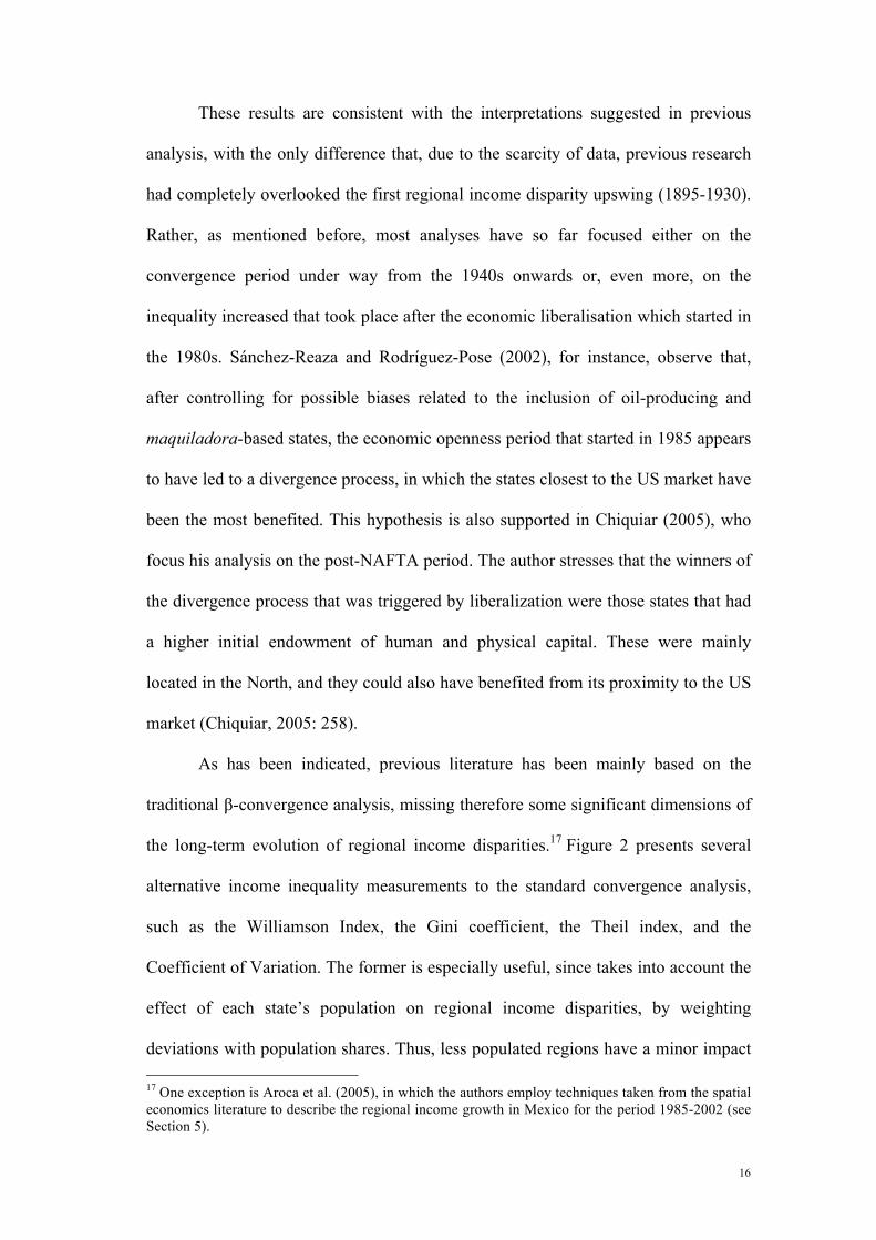
These results are consistent with the interpretations suggested in previous

analysis, with the only difference that, due to the scarcity of data, previous research

had completely overlooked the first regional income disparity upswing (1895-1930).

Rather, as mentioned before, most analyses have so far focused either on the

convergence period under way from the 1940s onwards or, even more, on the

inequality increased that took place after the economic liberalisation which started in

the 1980s. Sánchez-Reaza and Rodríguez-Pose (2002), for instance, observe that,

after controlling for possible biases related to the inclusion of oil-producing and

maquiladora-based states, the economic openness period that started in 1985 appears

to have led to a divergence process, in which the states closest to the US market have

been the most benefited. This hypothesis is also supported in Chiquiar (2005), who

focus his analysis on the post-NAFTA period. The author stresses that the winners of

the divergence process that was triggered by liberalization were those states that had

a higher initial endowment of human and physical capital. These were mainly

located in the North, and they could also have benefited from its proximity to the US

market (Chiquiar, 2005: 258).

As has been indicated, previous literature has been mainly based on the

traditional β-convergence analysis, missing therefore some significant dimensions of

the long-term evolution of regional income disparities.17 Figure 2 presents several

alternative income inequality measurements to the standard convergence analysis,

such as the Williamson Index, the Gini coefficient, the Theil index, and the

Coefficient of Variation. The former is especially useful, since takes into account the

effect of each state’s population on regional income disparities, by weighting

deviations with population shares. Thus, less populated regions have a minor impact                                                                                                                17 One exception is Aroca et al. (2005), in which the authors employ techniques taken from the spatial economics literature to describe the regional income growth in Mexico for the period 1985-2002 (see Section 5).

  17

in the index (and vice versa).18 Although the general trend is still the same as in the

standard deviation, this index would suggest a slightly interruption of the

convergence process during the 1950s. This may be explained for two main reasons.

The first one is the comparatively good performance of Mexico City, by far the most

populated region of the country (it concentrated 11.8% and 14.0% of national

population in 1950 and 1960 respectively), and whose GDP per capita, relative to the

national average, increased from 2.71 in 1950 to 2.76 in 1960. The second reason is

the low population density of some of the rich states that were performing worse than

the national average, such as Baja California Norte (with 0.8% and 1.4% of the

national population in 1950 and 1960), Baja California Sur (0.2% in both years), and

Quintana Roo (with 0.10% and 0.14% of the national population in 1950 and 1960).

These states went from having a relative GDP per capita of 2.96, 1.22, and 1.99 in

1950 to 1.89, 0.96 and 0.50 in 1960, respectively. By contrast, during the 1960s

Mexico City’s GDP per capita converged with the national average (from 2.76 in

1960 to 1.95 in 1970), as did other highly populated rich states, such as Nuevo León,

which had a relative GDP per capita of 2.13 in 1960, and 1.69 in 1970.

                                                                                                               18 The Williamson index, proposed in Williamson (1965), is calculated as follows:

!" =  !!!!

− 1! !!!!

!

!!!

 

where y is income per capita, p is population, and i and m refer to the i-region and the national total, respectively.  

  18

Source: See text

Both the Gini coefficient and the Theil index increase with income inequality,

and their values range from 0 to 1. Once again, a N-shape pattern emerges in the long

run. In fact, the trend shown by both indices is very similar, and follows closely the

evolution of the Williamson Index. The earlier twentieth century remains as the

period of fastest regional income divergence, and the maximum levels of inequality

were reached in 1940, much later than in most industrialized economies or Spain but

earlier than in other European peripheral countries, such as Italy or Portugal.19 The

levels of the Gini and Theil indices in Mexico are relatively high in comparison with

those found in the international literature. For instance, the maximum value of the

Gini index in Italy, Spain and Portugal in the long term was around 0.21, i.e. half of

                                                                                                               19 In Spain, the Gini index of regional inequality reached its maximum in 1920, in Italy in 1950 and in Portugal in 1970 (Herranz-Loncán and Martínez-Galarraga, 2013:7).

0

0.1

0.2

0.3

0.4

0.5

0.6

0.7

0.8

0.9

1

0

0.05

0.1

0.15

0.2

0.25

0.3

0.35

0.4

1895 1900 1910 1921 1930 1940 1950 1960 1970 1980 1990 2000 2010

Will

iam

son

inde

x an

d C

V

The

il an

d G

ini

Figure 2 Inequality index: Theil, Gini, Williamson and Coefficient of Variation,

1895-2010.

Theil Gini Williamson Coefficient of Variation

  19

the maximum value reached in the Mexican case. The Theil index offers similar

results: while the maximum value in the Mexican case was close to 0.25, the Italian,

Spanish and Portuguese maximum values were 0.07, 0.09, and 0.08 respectively

(Herranz-Loncán and Martínez-Galarraga, 2013:7).20 It is also interesting to mention

that while in Mexico the inequality peak is observed in 1940, in the industrialised

countries, this peak has been observed during the 19th century. In this sense, the

Mexican case could slightly match with some peripherals European economies such

as Italy and Spain (Herranz-Loncán and Martínez-Galarraga, 2013). Finally, the

trend followed by the Coefficient of Variation is also the same as in the other

indicators. The international comparison of the CV levels reinforces the idea that

Mexico had higher levels of regional income inequality than the core economies.

Following Crafts (2005), Britain’s CV values, which have been regularly used as a

reference for the core economies, ranged between 0.10 and 0.25 in the long term

(1871-2001). Meanwhile, in the Mexican case CV values have ranged from 0.39 to

0.83.

Figure 3 shows the Herfindahl-Hirschman Index (HHI) of Mexican regional

incomes and the share of Mexico City within the national total GDP. The HHI offers

an alternative approach to the regional income disparities, since does not take into

account the state relative GDP per capita, but the share of each state within national

GDP, measuring therefore the level of spatial concentration of national income. The

HHI is defined as:

                                                                                                               20 Differences in the number and scale of the spatial units in each country are a potential limitation in this comparison. However, the number of Mexican states (36) lies in between the number of Spanish provinces (50) and the number of Portuguese districts (18) and Italian regions (19).

  20

!!! =  !!"!!"!

!!!

!!

!!!

(1)

where Xij is the GDP for region i and sector j.

This index ranges from 1 (when all activity is concentrated in one region) to

1/n (when the activity is equally distributed among the n regions of a country). In

Mexico, the index follows an ‘inverted-U’ pattern, in which the divergence process

of the period 1980-2010 is missing. In addition, the initial process of increasing

concentration extends until the 1960s, and not until the 1940s as in the case of the

previous indices. Both differences respond to one fact: the economic importance of

Mexico City, the biggest economic centre of the country. As Figure 3 shows, there is

a close correlation between both series.21

Source: See text

                                                                                                               21 This is rather usual in countries in which one economic centre concentrates a large part of total GDP. See, for instance, the case of Chile and its capital Santiago (Badia-Miró, 2014).

0.00

0.02

0.04

0.06

0.08

0.10

0.12

0.14

0.16

0.18

0

5

10

15

20

25

30

35

40

1895 1900 1910 1921 1930 1940 1950 1960 1970 1980 1990 2000 2010

H-H

Inde

x

% o

f nat

iona

l GD

P

Figure 3 Herfindahl-Hirschman Index, 1895-2010 and the Share of Mexico City GDP in

national GDP

Mexico City Share Herfindahl-Hirschman Index

  21

The trend displayed by the HHI, together with Mexico City’s GDP share,

complements the description made in Section 2. Previous literature has insisted that

the ISI model (1930-1980) boosted the concentration of economic activity in Mexico

City. However, the figure shows that this process started earlier, in the 1910s, during

the export-led growth model. Concentration in the capital reached its maximum in

1960, and the sudden decrease of the HHI and the Mexico City’s GDP share during

the 1960s can be partially explained by the behaviour of the State of Mexico, which

was by then becoming, to a large extent, an extension of Mexico City. So, while

Mexico City lost 10.7 percentage points of participation in the national GDP from

1960 to 1970, the State of Mexico won 4.8 points in the same period.22

Things were completely different from 1980s onwards, when both Mexico

City’s and the State of Mexico’s GDP shares fell. From 1980 to 2010, they lost 7.6

and 1.2 percentage points of participation in national GDP, respectively. On the

contrary, the ‘winners’ in this period, as mentioned before, have been those states

that could benefit most from the economic openness policy. The main ones were the

north border states, led by Nuevo León, which won 2 points of national GDP since

1980, and also some central and southern states, such as Guanajuato, Querétaro and

Quintana Roo, which won 1.2, 0.9 and 1.2 percentage points of participation in

national GDP from 1980 to 2010. In Guanajuato and Querétaro, large foreign

investment has contributed to the development of the capital-intensive industrial

sector, whereas the Quintana Roo case has benefited from the development of

tourism.

Summing up the evidence in Figure 1 to 3, it is interesting to observe that the

increasing concentration of economic activity in Mexico City was accompanied, at                                                                                                                22 The rest of the Mexico City’s GDP share lost was distributed among several states, causing marginal changes in theirs GDP shares. The only exception to this pattern was the state of Jalisco, which won 2.5 points within national GDP in the same period.

  22

least since 1940, by a regional convergence process, which brought the southern

regions close to Mexico City in terms of average productivity. There are two

potential explanations of this convergence. Firstly, the concentration of industry in

Mexico City boosted the agglomeration of other activities with low productivity

levels, mainly within the service sector. Secondly, productivity in the primary sector

of the southern regions increased substantially, due to large migration flows to the

rest of the country. By contrast, the dispersion of industrial activity since the opening

of the economy has not been accompanied by income convergence, as in most

Western core economies, but by divergence, since industry tended to move towards

regions with relatively higher income per capita levels.

All the indices estimated so far have shown the evolution of regional income

inequality in Mexico in the long run. Nevertheless, as Quah’s (1993) seminal work

stressed, the classical convergence approach (Barro, 1991, and Barro and Sala-i-

Martin, 1992) is unable to capture some crucial features of regional inequality, such

as distributional dynamics. To address this issue, I present in the next paragraphs

some indicators of the regional distribution of economic activity in Mexico. To start

with, Figure 4 depicts a box-plots graph of regional GDP per capita figures. This

graph offers a very illustrative pattern of regional income distribution for those years

in which there was break in the evolution of regional income inequality (1900, 1940,

1980, 2000).23 For instance, during the early divergence process occurred between

1900 and 1940, the interquartile range increased, driven by the relatively poorer

states becoming even poorer. In fact, both the median income and the lower values

                                                                                                               23 Box-plot has three main components: the box, the whiskers, and the outliers (or the extreme values). The box is the interquartile range (IQ), being the distance between the 25th and 75th percentiles. The line within the box represents the median income. The whiskers represent the upper and lower values: the upper/lower value is the largest/smallest data point less/greater than or equal to the 75th/25th percentile value plus 1.5*(IQ). The values out of the whiskers are considered extreme values, and are plotted individually (i.e., these values are not considered in the percentiles).

  23

dropped in relative terms. On the other hand, quite surprisingly, the upper value,

together with the 75th percentile, remained fairly the same. The only group of states

that actually increased the income level were the top extreme values (Baja California

and Mexico City), which achieved, as mentioned before, values up to 3 or 4 times the

national average.

Figure 4 Box-plots estimates: 1900, 1940, 1980 and 2000. (Mexico=1)

Source: See text

Later on, the strong process of convergence between 1940 and 1980 is also

reflected in the main components of the 1980’s box-plot. Not only the interquartile

range is the narrowest over the long run, but also the lowest and upper values,

including the extreme values (in which only Mexico City remains), tended to

concentrate around the national average. This suggests that σ-convergence was

driven by both the poorer states improving their economic performance and the

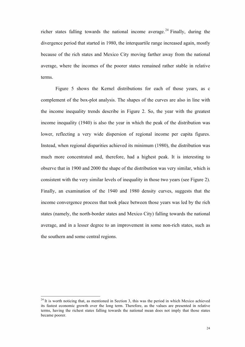
  24

richer states falling towards the national income average.24 Finally, during the

divergence period that started in 1980, the interquartile range increased again, mostly

because of the rich states and Mexico City moving farther away from the national

average, where the incomes of the poorer states remained rather stable in relative

terms.

Figure 5 shows the Kernel distributions for each of those years, as c

complement of the box-plot analysis. The shapes of the curves are also in line with

the income inequality trends describe in Figure 2. So, the year with the greatest

income inequality (1940) is also the year in which the peak of the distribution was

lower, reflecting a very wide dispersion of regional income per capita figures.

Instead, when regional disparities achieved its minimum (1980), the distribution was

much more concentrated and, therefore, had a highest peak. It is interesting to

observe that in 1900 and 2000 the shape of the distribution was very similar, which is

consistent with the very similar levels of inequality in those two years (see Figure 2).

Finally, an examination of the 1940 and 1980 density curves, suggests that the

income convergence process that took place between those years was led by the rich

states (namely, the north-border states and Mexico City) falling towards the national

average, and in a lesser degree to an improvement in some non-rich states, such as

the southern and some central regions.

                                                                                                               24 It is worth noticing that, as mentioned in Section 3, this was the period in which Mexico achieved its fastest economic growth over the long term. Therefore, as the values are presented in relative terms, having the richest states falling towards the national mean does not imply that those states became poorer.

  25

Figure 5 Kernel distribution estimates: 1900, 1940, 1980 and 2000

Source: See text

The Kernel distributions also show that a few states always had levels of

income significantly higher than the rest of the country, causing the rise, though in

different degrees throughout the period, of the twin peaks described in Quah (1997).

This was specially marked in 1940 (the year of the highest level of income

inequality), in which the GDP per capita of Mexico City and Baja California reached

their maximum relative value (3.84 and 4.29 times the national GDP per capita,

respectively). This is reflected in a long right-tail of the distribution, which was

accompanied by a relatively long left-side, suggesting that 1940 was also the year in

which the poorest states’ relative position was worst. By contrast, although it is also

clearly bi-modal, the 1980 distribution is the narrowest. Once again, this reflects the

relative high level of the GDP per capita of Mexico City. The new divergence

  26

process from the 1980s onwards is once more reflected in a lower peak and an

increasing dispersion of the right tail of the distribution.

Kernel densities provide relevant information for a complete understanding of

income distribution, but they do not give information on the transition from one

snapshot to another (Aroca et al., 2005:349). It would be important, for instance, to

know if the states at the end of the right tail of the distribution were always the same,

or whether there is a random behaviour, with states moving up and down the

distribution. In order to provide an insight of the states’ rank mobility, Figure 6

presents the Spearman and Kendall’s τ-statistic.25 The Spearman correlation and the

Kendall’s τ-statistic range from -1 to 1. In both cases, the higher the coefficient, the

lower the rank mobility (being 1 the value representing no mobility).26 In the

Mexican case, rank mobility was very low in the long run, which is consistent with

the general picture provided in Table 1, and supports the idea of a persistent north-

south regional income division. Furthermore, there is not a clear correlation between

the periods of σ-convergence or divergence and the evolution of rank mobility.

While all income dispersion indices confirm the N-shape trend in the long run, both

the Spearman and Kendall τ-statistics experience a constant increase. The only

exception is the period of stagnation or slight decrease of the indices from the 1980s

to the 2000s, which could be related to the process of economic openness and the

                                                                                                               25 The Spearman coefficient of correlation is calculated as: ! = 1 −   !   !!

!  (!!!!), where n is the size of the

sample, and d is the difference between the rank scores of two variables X and Y (in our case, the income rank in two different periods). Kendall’s τ-statistic considers the degree of concordance in the rankings of all pairs of observations for two variables. In the context of regional income mobility, the first variable would be the regional incomes for the initial year, while the second would be the incomes in the end year of the interval period. If two regions have the same relative rankings in both periods that pair is said to be concordant. However, if the relative rankings of the two switch over the interval, then the pair is discordant. Kendall’s τ- statistic is measured as: ! = !!!!!

(!!!!) !, where n is the

number of observations, !! is the number of concordant pairs, and !! the number of discordant pairs. With n observations there are (n2 − n)/2 pairwise comparisons to be made. 26 In the Spearman coefficient, having a !!=0 leads to a ! = 1, while in the Kendall’s τ-statistic, having a Nc=(n2 – n)/2, and therefore a Nd=0, means a value of τ =1.

  27

cases of successful states that might be affecting the national ranking (such as

Guanajuato, Querétaro, Quintana Roo, and some north border states which were

‘falling-behind’ during the ISI period).

Source: See text

4. A spatial-econometrics analysis: Moran’s I

This section aims at testing, through the estimation of the Moran’s I statistic,

whether the distribution of regional income has been characterized by statistically

significant spatial autocorrelation over the period under study. High spatial

correlation would be associated to a high level of spatial clustering of either rich or

poor regions. When there are significant levels of spatial clustering, it means that the

income observed in one state is relatively close to the income of the neighbouring

states. In the opposite case, in the absence of statistical significant correlation, the

0.00

0.10

0.20

0.30

0.40

0.50

0.60

0.70

0.80

0.90

1.00

1895 1900 1910 1921 1930 1940 1950 1960 1970 1980 1990 2000 2010

Figure 6 Spearman and Kendall's τ-statistic, 1895-2010

Spearman Kendall's t-statistic

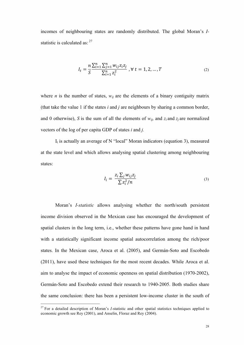
  28

incomes of neighbouring states are randomly distributed. The global Moran’s I-

statistic is calculated as: 27

!! =!!

!!"!!!!!!!!

!!!!

!!!!!!!

  ,∀  ! = 1, 2,… ,! (2)

where n is the number of states, wij are the elements of a binary contiguity matrix

(that take the value 1 if the states i and j are neighbours by sharing a common border,

and 0 otherwise), S is the sum of all the elements of wij, and zi and zj are normalized

vectors of the log of per capita GDP of states i and j.

It is actually an average of N “local” Moran indicators (equation 3), measured

at the state level and which allows analysing spatial clustering among neighbouring

states:

!! =  !! !!"!!!

!!!/! (3)

Moran’s I-statistic allows analysing whether the north/south persistent

income division observed in the Mexican case has encouraged the development of

spatial clusters in the long term, i.e., whether these patterns have gone hand in hand

with a statistically significant income spatial autocorrelation among the rich/poor

states. In the Mexican case, Aroca et al. (2005), and Germán-Soto and Escobedo

(2011), have used these techniques for the most recent decades. While Aroca et al.

aim to analyse the impact of economic openness on spatial distribution (1970-2002),

Germán-Soto and Escobedo extend their research to 1940-2005. Both studies share

the same conclusion: there has been a persistent low-income cluster in the south of                                                                                                                27 For a detailed description of Moran’s I-statistic and other spatial statistics techniques applied to economic growth see Rey (2001), and Anselin, Floraz and Rey (2004).

  29

the country during the entire period under study. Nevertheless, Aroca et al. (2005) do

not find statistically significant spatial autocorrelation in other areas of the country,

while Germán-Soto and Escobedo observe the existence of high-income clusters of

some northern and central estates. This difference might be explained by the

different GDP per capita database used by those authors. Aroca et al. (2005)

introduced several corrections to the INEGI database, mainly related to the allocation

of oil production, and also to the population data of some particular states in some

years. Instead, Germán-Soto and Escobedo (2011) used the database presented in

Germán-Soto (2005), in which, as mentioned before, there was no correction for oil

production.

In this paper, I extend the time span further to cover all the period 1895-2010.

In addition, I use a different database, which excludes oil production for the entire

period by applying a homogenous methodology (see Aguilar-Retureta, 2015). The

results are shown in Figure 7 (global Moran’s I estimate) and Map 2 (local Moran’s I

–clustering-). 28 As can be seen in the figure, the global level of spatial

autocorrelation decreased at the beginning of the period to remain rather constant

from 1910 onwards. The relatively high value of the global Moran’s I in 1895 can be

explained, essentially, by the presence of a cluster of high-income states in the north

(Baja California Norte, Sonora and Sinaloa) which has disappeared from 1900 on.

After 1900 no other significant high-income cluster of states appeared in Mexico,

and the levels of spatial autocorrelation remained rather low, being mainly explained

by similarities among neighbouring (poor) southern states, see Map 2. Unlike what

                                                                                                               28 As my state GDP per capita estimates for the period from 1895 to 1930 consider both Baja California territory (North and South) as a single state, as well as Yucatan and Quintana Roo (see Aguilar-Retureta, 2015), I have removed, from the Moran’s I analysis, the Baja California South and Quintana Roo states for that period. The other alternative is to assign the same income values to Baja California North and Baja California South, and to Yucatan and Quintana Roo. This strategy, however, could bias the Moran’s I results, since it would artificially impose perfect spatial income autocorrelation between two pairs of neighbouring states.

  30

has happened with income inequality, the low level of autocorrelation was not

significantly affected by changes in the economic policy model over the long term.

Source: See text

In order to illustrate spatial autocorrelation, Map 2 plots the statistically

significant income clusters for the following benchmark years: 1900, 1940, 1980 and

2000. The maps confirm that, despite their relatively good economic performance,

north-border states have not been consolidated as a rich cluster through the entire

period. For a north-border income cluster to emerge it would have been necessary,

due to the contiguity technique used as the basis of the spatial weighting matrix, not

only to have a significant spatial income autocorrelation across the north-border

states themselves, but also with their neighbouring states, namely the ‘second-line’

northern states (Sinaloa, Durango, Zacatecas and San Luis Potosí). This condition

was not met during the period under study. Instead, spillovers form the north-border

states to the ‘second line’ northern states has not been strong enough to boost a

statistically significant high-income cluster in the northern region. On the contrary,

0.00

0.10

0.20

0.30

0.40

0.50

0.60

1895 1900 1910 1921 1930 1940 1950 1960 1970 1980 1990 2000 2010

Figure 7 Global Moran's I (weighted by contiguity), 1895-2010

  31

income levels decreased rapidly with the distance from the border (See Table 1),

which is consistent with the fact that the relatively good economic performance of

the north-border states is largely related to their integration with the US market. In

this sense, Hanson (2001), using data on the 10 major Mexican-US border-city pairs,

has observed that the growth of export manufacturing in Mexico can account for a

substantial portion of employment growth in US border cities between 1975 and

1997.29 In other words, the backward and forward linkages of the main economic

activity of northern regions (manufacturing) have been largely located in the US

market, especially since the increase in economic openness that started in the mid-

1980s.

By contrast, the existence of a persistent poor income cluster formed by the

southern states is unquestionable.30 This finding is consistent with Aroca et al.’s

(2005) suggestions for the early years of economic openness (1985–2002). These

authors consider the consistently poor income of the southern cluster as the central

element behind the divergence process that has taken place since the beginning of the

liberalization process and, especially, since the signature of NAFTA (Aroca et al.,

2005: 372). However, Map 2 indicates that the poor-income clustering of the

southern states has not been associated to a particular economic model but has been a

persistent feature of the country’s regional distribution, in which the southern region

seems to be trapped in a long run dynamic of poor economic performance.

                                                                                                               29 By contrast, the author did not find statistically significant correlation between local employment in the U.S. interior cities and Mexican export production (Hanson, 2001: 285). 30 The case of Querétaro in 1940 (light-red state) is a particular case of one rich state (Querétaro) surrounded by very poor states. By 1940, Querétaro had a GDP per capita 1.16 times as the national one. On the other hand, its neighbouring states: Hidalgo, San Luis Potosí, Guanajuato and the State of Mexico had: .51, .56, .50, and .49, respectively.

  32

Map 2 Local Moran’s I. Significant Clustering Maps: 1900, 1940, 1980 and 200031

1900 1940

1980 2000

Source: Own elaboration, using GeoDa

Map 2 also shows that Mexico City, despite its historical economic

dynamism, has been unable to foster the formation of a statistically significant

cluster in the centre of the country. In other words, Mexico City’s economic

dynamism has not been strong enough to spread to the neighbouring states, not even

                                                                                                               31 These clusters are derived from the local Moran’s I- statistic and are statistically significant at the 5 per cent.

Not Significant

High-High

Low-Low

Low-High

High-Low

  33

during the ISI period, when economic concentration in Mexico City achieved its

maximum (see Figure 3). Similarly, the recent dynamism of Quintana Roo has not

affected its neighbouring states (Yucatán and Campeche). 32 These examples,

together with the north-border states experience, suggest that, in the Mexican case,

having rich neighbours does not involve a greater chance of being prosperous.33

5. Concluding remarks

This paper has offered new evidence of the evolution and dynamics of

regional inequality in Mexico over the long run (1895-2010). The evolution of

spatial disparities in Mexico has some specific features that distinguish it from

previous analyses of the core economies. .

Mexican regional inequality has been characterized by a long-lasting north-

south regional income division. Against this persistent background, over time

Mexican regional inequality has followed an ‘N’-shape trend, which largely matches

the different economic models that have been adopted in Mexico. Thus, the years of

export-led growth, from the late 19th to the 1930s, were characterized by a strong

regional divergence process. By contrast, during the ISI period (1940-1980), there

was intense convergence among the Mexican regional economy and, finally, in the

context of increasing international integration that started in the 1980s, divergence

has again been the norm. Beyond those fluctuations, and regardless the historical

period under consideration, regional inequality in Mexico has always been

comparatively high.                                                                                                                32 This is largely a consequence of the location-specific character of tourism, which is the main engine behind Quintana Roo’s economic growth. 33 Recently, Tirado and Badia-Miró (2014) have also used this technique for the Iberian case from an historical perspective. The authors conclude that, unlike Mexico, Iberia has experienced an increasing spatial correlation in the long run, which can be seen in the permanent increase in the values of both the global and the local Moran’s I statistics (led by the expansion of both rich and poor regions). However, they also find an administrative capital effect with no diffusion to the closest regions, as in the case of Mexico City.

  34

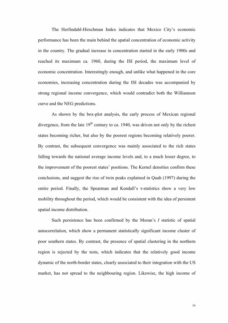
The Herfindahl-Hirschman Index indicates that Mexico City’s economic

performance has been the main behind the spatial concentration of economic activity

in the country. The gradual increase in concentration started in the early 1900s and

reached its maximum ca. 1960, during the ISI period, the maximum level of

economic concentration. Interestingly enough, and unlike what happened in the core

economies, increasing concentration during the ISI decades was accompanied by

strong regional income convergence, which would contradict both the Williamson

curve and the NEG predictions.

As shown by the box-plot analysis, the early process of Mexican regional

divergence, from the late 19th century to ca. 1940, was driven not only by the richest

states becoming richer, but also by the poorest regions becoming relatively poorer.

By contrast, the subsequent convergence was mainly associated to the rich states

falling towards the national average income levels and, to a much lesser degree, to

the improvement of the poorest states’ positions. The Kernel densities confirm these

conclusions, and suggest the rise of twin peaks explained in Quah (1997) during the

entire period. Finally, the Spearman and Kendall’s τ-statistics show a very low

mobility throughout the period, which would be consistent with the idea of persistent

spatial income distribution.

Such persistence has been confirmed by the Moran’s I statistic of spatial

autocorrelation, which show a permanent statistically significant income cluster of

poor southern states. By contrast, the presence of spatial clustering in the northern

region is rejected by the tests, which indicates that the relatively good income

dynamic of the north-border states, clearly associated to their integration with the US

market, has not spread to the neighbouring region. Likewise, the high income of

  35

Mexico City has not radiated to other central states, not even during the ISI period, in

which economic activity greatly tended to concentrate around this city.

This first approach to regional inequality will be the basis for further

explanatory analysis, and the test of several hypotheses that may explain the

particular features of regional economic inequality in Mexico and other peripheral

economies. What role has played the industrialisation process and its location in the

evolution of regional inequality? Is there a structural differential driving this

tendency? Or, are agglomeration economies significant in this process? These are

some of the questions that will be addressed in future research.

6. Bibliography Aguilar, I. (1993), “Descentralización industrial y desarrollo regional en México”, El

Colegio de México, México. Aguilar-Retureta, J. (2015), “The GDP per capita of the Mexican regions (1895-1930): new

estimates”, Revista de Historia Económica – Journal of Iberian and Latin American Economic History (forthcoming).

Anselin, L., Florax, R., Rey, S. (2004), Advances in spatial econometrics. Methodology, tools and applications. Springer-Verlag, Berlin.

Aroca, P., Bosch, M., and Maloney, W. (2005), “Spatial Dimensions of Trade Liberalization and Economic Convergence: Mexico 1985-2002”, The World Bank Economic Review, 19, 3, pp. 345-378.

Badia-Miró, M. (2014) “The evolution of the localization of economic activity in Chile in the long run: a case of extreme concentration”, Paper presented at the 4th Latin American Economic History Congress (CLADHE), Colombia.

Badia-Miró, M., Guilera, J., and Lains, P. (2012), “Regional Incomes in Portugal: Industrialisation, Integration and Inequality, 1890-1980”, Revista de Historia Económica, 30, 02, pp. 225-244.

Barro, R. (1991), “Economic growth in a cross-section of countries”, Quarterly Journal of Economics, 106, 2, pp. 407-443.

Barro, R., and Sala-i-Martin, X. (1992), “Convergence”, Journal of Political Economy, 100, 2, pp. 223-251.

Bértola, L., and Ocampo, J. (2010), “Desarrollo, vaivenes y desigualdad. Una historia económica de América Latina desde la independencia”, Secretaría General Iberoamericana, Madrid.

Bosch, M., Aroca, P., Fernández, I., and Azzoni, C. (2003), “Growth Dynamics and Space in Brazil”, International Regional Science Review, 26, 3, pp. 393-418.

Brock, G. and Germán-Soto, V. (2013), “Regional industrial growth in Mexico: Do human capital and infrastructure matter?”, Journal of Policy Modeling, 35, pp. 228-242.

  36

Carrion-I-Silvestre, J., and German-Soto, V. (2007), “Stochastic Convergence amongst Mexican States”, Regional Studies, 41, 4, pp. 531-541.

Caruana-Galizia, P. (2013), “Indian regional income inequality: estimates of provincial GDP, 1875-1911”, Economic History of Developing Regions, 28:1, pp. 1-27.

Cerutti, M. (1992), “Burguesía, capitales e industria en el Norte de México: Monterrey y su ámbito regional, 1850-1910”, Ed. Alianza, México.

Chiquiar, Daniel (2005), “Why Mexico’s regional income convergence broke down”, Journal of Development Economics, 77, pp. 257-275.

Combes, P., Lafourcade, M., Thisse, J., Toutain, J. (2011), “The rise and fall of spatial inequalities in France: A long-run perspective”, Explorations in Economic History, 48, pp. 243-271.

Crafts, N. (2005), “Regional GDP in Britain, 1871-1911: some estimates”, Scottish Journal of Political Economy, vol. 52, No. 1, pp. 54-64.

Crafts, N. and Mulatu, A. (2005), “What explains the location of industry in Britain, 1871–1931?”, Journal of Economic Geography, 5, pp. 499-518.

Dobado R. y Marrero G. (2005), “Corn Market Integration in Porfirian Mexico”, The Journal of Economic History, vol. 65, No. 1, pp. 103 – 128.

El Colegio de México (México, 1964), Estadísticas Económicas del Porfiriato: Fuerza de trabajo y actividad económica por sectores.

ECLAC (2014), “Cambio estructural para la igualdad. Una visión integrada del desarrollo”. Santiago de Chile, CEPAL.

E. DeGolyer (1993), "Production of the Mexican Oil Field, 1901-1920" In: Brown, Jonathan C. Oil and Revolution in Mexico.

Enflo, K. and Rosés, J. (2014), “Coping with regional inequality in Sweden: structural change, migrations, and policy, 1860-2000”, The Economic History Review, online available version (June).

Epstein, P., Howlett, P. and Schulze, M. (2003), “Distribution dynamics: stratification, polarization, and convergence among OECD economies, 1870-1992”, Explorations in Economic History, 40, pp. 78-97.

Esquivel, G. (1999), “Convergencia Regional en México, 1940-1995”, El Trimestre Económico, LXVI, 264, pp. 725-761.

Esquivel, G. (2002), “New Estimates of Gross State Product in Mexico, 1940-2000”, Mimeo. El Colegio de México.

Felice, E. (2011), “Regional value added in Italy, 1891-2001, and the foundation of a long-term picture”, The Economic History Review, 64, 3, pp. 929-950.

Geary, F. and Stark, T. (2002), “Examining Ireland's Post-Famine Economic Growth Performance”, The Economic Journal, 112, 482, pp. 919-935.

Geary, F. and Stark, T. (2015), “Regional GDP in the UK, 1861-1911: new estimates”, The Economic History Review, 68, 1, pp. 123-144.

Germán-Soto, V. (2005), “Generación del Producto Interno Bruto mexicano por entidad federativa, 1940-1992”, El Trimestre Económico, LXXII, 287, pp. 617-653.

Germán-Soto, V. and Escobedo, J. (2011), “¿Ha ampliado la liberalización comercial la desigualdad económica entre los estados mexicanos? Un análisis desde la perspectiva econométrico-espacial”, Economía Mexicana. Nueva Época, XX, 1, pp. 37-77.

Gómez-Galvarriato, A. (2002), “Measuring the Impact of Institutional Change in Capital-Labor Relations in the Mexican Textile Industry, 1900-1930”. In J. Bortz and S. Haber (Eds.), The Mexican Economy, 1870-1930. Essays on the Economic History of Institutions, Revolution, and Growth. (pp. 289-323).

  37

Gutiérrez Requenes, M. (1969), Producto Interno Bruto y Series Básicas 1895-1967, Mimeo, Banco de México.

Haber, S. (1989), Industry and Underdevelopment: The Industrialization of Mexico, 1890-1940, Stanford University Press.

Haber, S. (2010), “Mercado Interno, Industrialización y Banca, 1890-1929”, In Historia Económica General de México: de la Colonia a nuestros día, Kuntz, Sandra (coord.), El Colegio de México.

Hanson, G. (1998a), “North American Economic Integration and Industry Location”, Oxford Review of Economic Policy, 14, pp. 30-44.

Hanson, G. (1998b), “Regional Adjustment to Trade Liberalization”, Regional Science and Urban Economics, 28, pp. 419-444.

Hanson, G. (2001), “U.S.-Mexico Integration and Regional Economies: Evidence from Border-City Pairs”, Journal of Urban Economics, 50, pp. 259-287.

Henning, M., Enflo, K., Andersson, F. (2011), “Trends and cycles in regional economic growth. How spatial differences shaped the Swedish growth experience from 1860-2009”, Explorations in Economic History, 48, pp. 538-555.

Herranz-Loncán, A., and Martínez-Galarraga, J. (2013), “The dynamics of the regional distribution of income in Portugal, Spain and Italy since the late 19th century”, Unpublished research paper.

Hernández, E. (1980), “Economías externas y el proceso de concentración regional de la industria en México”, El Trimestre Económico, 47, pp. 119-157.

Jordaan, J.A. and Sanchez-Reaza, J. (2006), “Trade liberalization and location: Empirical evidence for Mexican manufacturing industries 1980-2003”, The Review of Regional Studies, 36 p. 279-303.

Kim, S. (1998), “Economic Integration and Convergence: U.S. Regions, 1840-1987”, The Journal of Economic History, 58, 3, pp. 659-683.

Kim, S. (1999), “Regions, resources, and economic geography: Sources of U.S. regional comparative advantage, 1880-1987”, Regional Science and Urban Economics, 29, pp. 1-3.

Klein, A. and Crafts, N. (2012), “Making sense of the manufacturing belt: determinants of U.S. industrial location, 1880–1920”, Journal of Economic Geography, 12, pp. 775-807.

Krugman, P. (1991), Geography and Trade, MIT Press, Cambridge, MA. Krugman, P., and Livas-Elizondo, R. (1996), “Trade policy and the third world metropolis”,

Journal of Development Economics, 49, pp. 147–150. Kuntz, S. (1999), “Los ferrocarriles y la formación del espacio económico en México, 1880-

1910”, In Sandra Kuntz and Priscilla Connoly (coords.), Ferrocarriles y obras públicas, El Colegio de México, Instituto Mora, El Colegio de Michoacán, Instituto de Investigaciones Históricas-UNAM, México.

Kuntz, S. (2010), “De las Reformas Liberales a la Gran Depresión, 1856 - 1929”, In Historia Económica General de México: de la Colonia a nuestros día, Kuntz, Sandra (coord.), El Colegio de México.

Kuntz, S. and Speckman, E. (2011)., “El Porfiriato”, In Nueva Historia General de México, Erik Velásquez García … [et al.], El Colegio de México.

Kuntz, S. (2014), “The contribution of exports to the Mexican economy during the first globalisation”, Australian Economic History Review, 54, pp. 95-119.

Martínez-Galarraga, J. (2012), “The determinants of industrial location in Spain, 1856–1929”, Explorations in Economic History, 49, pp. 255-275.

  38

Martínez-Galarraga, J., Rosés, J., and Tirado, A. (2013), “The long-term patterns of regional income inequality in Spain, 1860-2000”, Regional Studies, pp. 1-17.

Márquez, G. (2010), “Evolución y estructura del PIB, 1921-2010”, In Historia Económica General de México: de la Colonia a nuestros día, Kuntz, Sandra (coord.), El Colegio de México.

Pérez López, E. (1960), “El producto nacional” en México: cincuenta años de revolución”, vol. 1, pp. 571-592.

Puga, D. (1999), “The rise and fall of regional inequalities”, European Economic Review, 43, pp. 303-334.

Quah, D. (1993), “Empirical cross-section dynamics in economic growth”, European Economic Review, 37, pp. 426-434.

Quah, D. (1997), “Empirics for Growth and Distribution: Stratification, Polarization, and Convergence Clubs”, Journal of Economic Growth, 2, pp. 27-59.

Rey. S. (2001), “Spatial Empirics for Economic Growth and Convergence”, Geographical Analysis, 33, pp. 195-214.

Riguzzi, P (1995), “Inversión extranjera e interés nacional en los ferrocarriles mexicanos, 1880-1914” In Carlos Marichal (coord.) Las inversiones extranjeras en américa latina, 1850-1930. Nuevos debates y problemas en historia económica comparada, El Colegio de México, México.

Rosés, R., Martínez-Galarraga, J., and Tirado, D. (2010), “The upswing of regional income inequality in Spain (1860-1930)”, Explorations in Economic History, 47 pp. 244-257.

Rodríguez-Oreggia, E. (2005), “Regional disparities and determinants of growth in Mexico”, The Annals of Regional Science, 39, pp. 207-220.

Ruiz Ochoa, W. (2010), “Convergencia económica interestatal en México, 1900-2004”, Análisis Económico, XXV, pp. 7-34.

Sánchez-Reaza, J., and Rodríguez-Pose, A. (2002), “The impact of trade liberalization on regional disparities in Mexico”, Growth and Change, 33, pp. 72-90.

Tirado, D. and Badia-Miró, M. (2014), “New Evidence on Regional Inequality in Iberia (1900-2000)”, Historical Methods: A Journal of Quantitative and Interdisciplinary History, 47:4, pp. 180-189.

Williamson, J. (1965), “Regional inequality and the process of national development: a description of the patterns”, Economic Development and Cultural Change, 13:4, pp. 3-84.

World Bank (2014), World Development indicators database, http://data.worldbank.org/indicator (accessed: 23/01/2015).

Yamamoto, D. (2008), “Scales of regional income disparities in the USA, 1955-2003”, Journal of Economic Geography, 8, pp. 79-103.