Multivariate Stochastic Volatility with Co-Heteroscedasticity 1 Joshua Chan Purdue University Arnaud Doucet University of Oxford Roberto Le´ on-Gonz´ alez National Graduate Institute for Policy Studies (GRIPS) and Rodney W. Strachan University of Queensland October 2018 1 The authors thank seminar participants at the 12 th RCEA Bayesian Workshop and the 4 th Hitotsubashi Summer Institute for helpful comments and suggestions. Roberto Le´on-Gonz´alez acknowledges financial support from the Nomura Foundation (BE-004). All errors are, of course, our own. 1
Transcript
Multivariate Stochastic Volatility with Co-Heteroscedasticity1
Joshua Chan
Purdue University
Arnaud Doucet
University of Oxford
Roberto Leon-Gonzalez
National Graduate Institute for Policy Studies (GRIPS)
and
Rodney W. Strachan
University of Queensland
October 2018
1The authors thank seminar participants at the 12th RCEA Bayesian Workshop and the 4th Hitotsubashi SummerInstitute for helpful comments and suggestions. Roberto Leon-Gonzalez acknowledges financial support from the NomuraFoundation (BE-004). All errors are, of course, our own.
1
ABSTRACT
This paper develops a new methodology that decomposes shocks into homoscedastic and het-
eroscedastic components. This specification implies there exist linear combinations of heteroscedas-
tic variables that eliminate heteroscedasticity. That is, these linear combinations are homoscedastic;
a property we call co-heteroscedasticity. The heteroscedastic part of the model uses a multivariate
stochastic volatility inverse Wishart process. The resulting model is invariant to the ordering of the
variables, which we show is important for impulse response analysis but is generally important for, e.g.,
volatility estimation and variance decompositions. The specification allows estimation in moderately
high-dimensions. The computational strategy uses a novel particle filter algorithm, a reparameteriza-
tion that substantially improves algorithmic convergence and an alternating-order particle Gibbs that
reduces the amount of particles needed for accurate estimation. We provide two empirical applications;
one to exchange rate data and another to a large Vector Autoregression (VAR) of US macroeconomic
variables. We find strong evidence for co-heteroscedasticity and, in the second application, estimate
the impact of monetary policy on the homoscedastic and heteroscedastic components of macroeconomic
It is now well recognised that the variance for many macroeconomic and financial variables change
over time. Many approaches have been proposed and employed to model this behaviour including Au-
toregressive Conditional Heteroscedasticity (ARCH) and Generalized ARCH (GARCH) models (Engle
(1982), Bollerslev (1986)) in which the variance of the reduced form errors is a deterministic function
of past residuals and variances. Another important class of models of the variance are the stochastic
volatility (SV) models. These differ from ARCH and GARCH models in that the conditional variance
is an unobserved Markov Process.
For univariate models, it has been found that SV models forecast better than GARCH in terms of
root mean squared forecast error and log-predictive scores for macro data (e.g. Chan (2013)) and in
terms of log Bayes factors for financial data (e.g. Kim , Shephard and Chib (1998)). Similar evidence is
found in multivariate models (e.g. Clark and Ravazzolo (2015)) where the SV specification provides the
advantage of more flexible models since the GARCH approach requires many simplifying restrictions
to ensure that the covariance matrix is positive definite.
In many applications, it is important to have an accurate estimate of the reduced form covariance
matrix, Σt, and of its stationary value E(Σt). Impulse response functions in VAR analysis of macroeco-
nomic data, for example, rely on decompositions of the reduced form covariance matrix (e.g. Hamilton
(1994, p.320)). To accurately report the impact of structural shocks requires a good estimate of the
covariance matrix. Another example is in portfolio allocation based on financial data.
If the order of the variables in a vector affects the estimates of its covariance matrix then we can
say that the estimation method is not invariant to ordering. An issue with the approaches employed
in most of the literature on multivariate stochastic volatility models (e.g. Primiceri (2005), Chib et al.
(2009)) is that they are not, in fact, invariant to ordering. A survey of the applied literature suggests
that a common specification is to use a Cholesky decomposition of Σt, and let each element of this
decomposition follow a Markov Process. However, this implies that the distribution of Σt and the
predictive distribution of yt depend on the ordering. An alternative approach to modelling multivariate
volatility uses factor models. Factor models also require restrictions to permit estimation and, again,
the most commonly employed restrictions on factor models are not invariant (Chan et al., (2018)).
Another feature of the multivariate SV models used in the literature is that they use a log-normal
distribution for the volatility. This specification implies that all moments of the volatility exist. In many
applications, particularly in finance, features of the data suggest that the distributions have heavy tails
and possibly few moments. To allow for the possibility of heavy tails, it is common to use Student’s-t
errors.
3
Another line of literature in modelling multivariate SV uses Wishart or inverted Wishart processes
(see, for example, Uhlig (1997), Philipov and Glickman (2006), Casarin and Sartore (2007), Asai and
McAleer (2009), Fox and West (2011), Triantafyllopoulos (2011), and Karapanagiotidis (2012)). A
feature of this approach is that the estimates are invariant to ordering. Inverted Wishart models also
allow for non-existence of higher moments and heavier tails. In a recent paper, Leon-Gonzalez (2018)
shows, in the univariate case, that Student’s-t errors are often not needed to model heavy tails when an
inverse gamma volatility process is used, but are very important when a log-normal volatility process is
used. The approach in this paper uses an inverse Wishart process but differs from the above approaches
in a number of respects. For example, the model is relatively unrestricted, computation is more efficient,
the stationary covariance matrix is estimated and the specification permits an interesting decomposition
of the errors into homoscedastic and heteroscedastic parts.
In this paper we propose inference on multivariate volatility in an Inverted Wishart SV model. The
resulting inference is invariant to ordering of the variables and allows for heavy tails and even non-
existence of higher order moments. We present a novel particle filter that samples all volatilities jointly
conditionally on the unknown parameters using Particle Gibbs (Andrieu et al. (2010)) with backward
sampling (Whiteley (2010)). The particle filter uses an approximation of the posterior distribution as
a proposal density, which allows us to substantially reduce the computation time in models of higher
dimension, and it is related to the ψ-Auxiliary Particle Filters studied in Guarniero et al. (2017).
We additionaly use the approximation of the posterior to find a reparameterization of the model that
substantially reduces the correlation between the latent states and the fixed parameters, which we
empirically find to speed up computation and thus contributes to the literature on parameterization in
state space and hierarchical models (e.g. Pitt and Shephard (1999), Papaspiliopoulos et al. (2007)).
We also propose to alternate the order in which the volatilities are generated, finding that this reduces
the number of particles needed for accurate estimation. Another important feature of our approach is
that the specification results in a reduction in the dimension of the latent variables, greatly improving
computation efficiency and permitting inference on potential co-heteroscedasticity. This allows us to
obtain new variance decompositions as well as new insights into the characteristics of the structural
shock and its impact on the variables of interest. Co-heteroscedasticity might also be relevant to find
portfolio allocations with thinner tails and constant variance returns.
The structure of the paper is as follows. Section 2 describes the model and the identification strategy.
Section 3 clarifies the difference between identifying assumptions and ordering of variables and presents
decompositions of impulse responses and the variance. Section 4 presents the particle filter to estimate
the likelihood while in Section 5 the particle Gibbs algorithm and tools for model comparison are
presented. Section 6 discusses two applications to real data, one to a large VAR of macroeconomic
4
variables and another one to returns of exchange rates.
2 Model and Identification Strategy
We consider the following model of stochastic volatility:
yt = βxt + et, with et ∼ N(0,Σt)
where β : r × kx, xt : kx × 1 and et : r × 1. The vector et can be decomposed into r1 heteroscedastic
errors (u1t : r1 × 1) and r2 homoscedastic errors (u2t : r2 × 1), with r = r1 + r2:
et = A1u1t +A2u2t =
(A1 A2
) u1t
u2t
= Aut (1)
We can then decompose Σt as:
Σt = var(et) = var(A1u1t)︸ ︷︷ ︸changing
+ var(A2u2t)︸ ︷︷ ︸constant
where as a normalization we fix cov(u1t, u2t) = 0 and var(u2t) = Ir22. Note that this implies that there
are r2 linear combinations of et which are homoscedastic. In particular, if the (r × r2) matrix A1⊥ lies
in the space of the orthogonal complement of A1, then the r2× 1 vector A′1⊥et has a constant variance.
We say then that the elements of the vector yt share heteroscedastic shocks, a property that we define
as co-heteroscedasticity in the following definition.
Definition 1 Let =t = (yt−1, yt−2, ..., xt, xt−1, ..., ) be all the information available up to period t. An
r × 1 vector yt with time variant conditional var-cov matrix (i.e. var(yt|=t) = Ω=t) is said to be co-
heteroscedastic if there exists a full rank matrix A1⊥ : r × r2 such that the vector A′1⊥yt has a constant
conditional var-cov matrix (i.e. var(A′1⊥yt|=t) = Ω0 for all t), with 0 < r2 < r. The largest possible
value of r2 for which this property holds is the co-heteroscedasticity order.
In our framework the heteroscedastic errors u1t have var(u1t) = K−1t , where Kt = Z ′tZt, and Zt is
a n× r1 matrix distributed as a Gaussian AR(1) process3:
Zt = Zt−1ρ+ εt vec(εt) ∼ N(0, Ir1 ⊗ In) (2)
2Because var(et) = Avar(ut)A′, it is not possible to identify var(ut) and A at the same time, hence the normalization.3This representation implies that n is an integer, but in Section 5 we will use an equivalent representation that allows
n to be continuous when n ≥ 2r1.
5
where ρ is diagonal r1 × r1 (with diagonal elements smaller than one in absolute value) and we assume
that vec(Z1) is drawn from the stationary distribution N(0, (Ir1 − ρ2)−1 ⊗ In). So var(et) = Σt can be
written as:
Σt = A1K−1t A′1 +A2A
′2 = A
K−1t 0
0 Ir2
A′, for A =
(A1 A2
)(3)
Because var(yt|xt) = E(Σt), it is possible to identify G = E(Σt), but restrictions are needed to identify
A = (A1, A2). For the purpose of identification, we assume that the time-varying component of Σt
has on average bigger singular values than the constant component. The reason for this assumption
is that it is well-known that stochastic volatility is empirically important, and therefore we introduce
K−1t into the model in the way that it will have the greatest impact, which is by interacting K−1t with
the largest singular values of G. To impose this assumption we use the singular value decomposition of
E(Σt) (SVD, e.g. Magnus and Neudecker (1999, p. 18)), which is given by:
G = E(Σt) = USU ′ = U1S1U′1 + U2S2U
′2 (4)
where U is a r×r orthogonal matrix such that U ′U = Ir, S = diag (s1, ..., sr) with s1 ≥ s2 ≥ ... ≥ sr ≥ 0,
and S1 contains the r1 biggest singular values, such that:
U =
(U1 U2
)S =
S1 0
0 S2
(5)
U1 : r × r1, U2 : r × r2, S1 : r1 × r1, S2 : r2 × r2
Let us standardize K−1t by defining Υ−1t = (n−r1−1)(I−ρ2)−1/2K−1t (I−ρ2)−1/2, such that E(Υ−1t ) =
Ir1 . We impose the identifying assumption by writing:
Σt = U1S1/21 Υ−1t S
1/21 U ′1 + U2S2U
′2 (6)
where we are also assuming that n > r1 + 1, so that E(Σt) is finite4. Comparing (3) and (6) we are
able to identify A1 and A2 as follows:
4Note that the variance of any element of K−1t will only be finite when n > r1 + 3 (e.g. Gupta and Nagar (2000,
p.113)), and so the restriction n > r1 +1 still allows for very fat tails. Also note that the marginal of any diagonal elementof K−1
t is an inverted Gamma-2 distribution (Bauwens et al. (1999, p.p. 292, 305 )) with (n− r1 + 1) degrees of freedom.Therefore, if n = r1 + 2 (which is the minimum value that we allow in this paper), the marginal of a diagonal element ofK−1
t will have only 3 degrees of freedom, implying that it has finite mean but not finite variance.
6
A1 =√
(n− r1 − 1)U1S1/21 (I − ρ2)−1/2 (7)
A2 = U2S1/22
We follow a Bayesian approach and put a prior directly on (G, ρ, n, β), where G enters the model
through (A1, A2). This framework allows for a Normal-Wishart prior on (β,G), which simplifies the
calculations in the context of estimating a large VAR. This prior allows for shrinkage, and implies that
the conditional posterior of β is normal with a mean and var-cov matrix which can be calculated without
inverting large matrices. In particular, the posterior mean and var-cov matrix of β can be calculated
by inverting matrices of order r1kx. This implies a reduction from rkx to r1kx.
The distribution for Kt implied by (2) is known in the literature as Wishart Autoregressive process
of order 1 (WAR(1)) and its properties are well established (e.g. Gourieroux et al. (2009), Koop et
al. (2011)). For example, the stationary distribution of Kt is a Wishart distribution with n degrees of
freedom and E(Kt) = n(I − ρ2)−1, and the conditional expectation of Kt|Kt−1 is equal to a weighted
average of Kt−1 and E(Kt):
E(Kt|Kt−1) = ρKt−1ρ+ (I − ρ2)1/2E(Kt)(I − ρ2)1/2
3 Invariance, Identification of Structural Shocks and Decom-
positions
When we refer to invariance to the ordering of the variables, we mean that the ordering of the variables
in the vector yt should not have any impact on inference. The ordering of the variables, understood
in this sense, is a concept that should be distinguished from the identifying assumption to obtain the
structural shocks, as any particular identifying assumption can be imposed regardless of the ordering
of the variables in the vector yt. For example, consider the identifying assumption that y1t is a slow
variable, such that it does not react contemporaneously to a shock to y2t. This assumption is normally
imposed by writing the reduced form shocks et = (e1t, e2t) as a function of orthogonal structural shocks
as follows:
7
e1t
e2t
=
p11 0
p21 p22
︸ ︷︷ ︸
P
ξ1t
ξ2t
, with PP ′ = var
e1t
e2t
= Σ =
σ11 σ12
σ12 σ22
The matrix P contains the parameters of interest and it is common to put a relatively non-
informative prior on them, say π(P ). However, the same identifying assumption can also be used
with the reverse ordering, first defining the following observationally-equivalent model with orthogonal
shocks denoted by (ξ2t, ξ1t):
e2t
e1t
=
p11 0
p21 p22
︸ ︷︷ ︸
P
ξ2t
ξ1t
, with P P ′ = var
e2t
e1t
= Σo =
σ22 σ12
σ12 σ11
where Σo is equal to Σ after reordering the rows and columns. After specifying a prior on P , say π(P ),
the model can be estimated, and the identifying assumption can be imposed ex-post by first reordering
the rows and columns of the estimated Σo = P P ′ to obtain an estimate of Σ, and then calculating its
Cholesky decomposition to obtain estimates of the structural parameters in P . However, unless both
π(P ) and π(P ) imply the same prior on Σ, these two approaches will give different results (Sims and Zha
(1998, eqns. 24-25, p. 961)), with the difference being very pronounced in the context of a large VAR
with stochastic volatility, as we illustrate in the empirical section. Whenever precise prior information
is available about P , it seems reasonable to put directly a prior on P . However, in most cases there is
not such prior information, and this is specially the case when a block identifying assumption is used
(as we do in Section 6.1, see also Zha (1999)), where a block of variables is assumed to react slowly,
without making any assumption about which variables are slower within the block.
Equations (1) and (7) imply that the heteroscedastic component of et can be obtained as ehett =
U1U′1et = H1et = A1u1t, such that yt can be decomposed into its heteroscedastic (yhett ) and ho-
moscedastic components (yhomt ). In the case of a VAR in which xt contains a constant and lags of yt,
the decomposition can be obtained by using the moving average representation:
where H2 = Ir−H1 = U2U′2. Note that yhett is a sum of only heteroscedastic shocks, and yhomt is a sum
of only homoscedastic shocks. After writing et in terms of orthogonal shocks et = Pξt, and using some
assumption to identify P , the impulse response function can be decomposed as:
IR(s; i, j) =∂yi,t+s∂ξjt
=∂yheti,t+s
∂ξjt+∂yhomi,t+s
∂ξjt= IRhet(s; i, j) + IRhom(s; i, j)
where the partial derivatives correspond to the (i, j) elements of ΨsP , ΨsH1P or ΨsH2P, respec-
tively, with Ψ0 = Ir. IRhet(s; i, j) can be interpreted as the impact of ξjt on yhett at horizon s, and
IRhom(s; i, j) can be interpreted in an analogous way. Equation (8) can also be used to obtain variance
decompositions, calculating the proportion of var(yt|yt−h), var(yhett |yt−h) or var(yhomt |yt−h) caused by
the structural shocks ξt or by the heteroscedastic shocks (u1t), as we illustrate in the empirical section.
Importantly, we can also calculate the proportion of the variance of the structural shock ξt caused by
the heteroscedastic shocks, by noting that ξt = P−1et = P−1(A1u1t+A2u2t), and therefore the variance
of the heteroscedastic component of ξt is var(P−1(A1u1t)) = var(P−1(H1et)) = P−1H1GH′1
(P−1
)′.
Finally, note that by decomposing yt into yhett and yhomt using equation (8), we can estimate how yt
would behave if there were only heteroscedastic shocks (i.e. u2t = 0 and yt = yhett ) or there were only
homoscedastic shocks (i.e. u1t = 0 and yt = yhomt ), as we illustrate in the empirical section.
4 Likelihood and Particle Filter
The value of the likelihood evaluated at the posterior means of the parameters can be used to calculate
the Bayesian Information Criterion (BIC) or the marginal likelihood (Chib and Jeliazkov (2001)) for
selecting r1. However, because the likelihood cannot be calculated in analytical form, we propose a
particle filter that provides a numerical approximation. This particle filter will also be a key ingredient
of the particle Gibbs algorithm that we use to sample from the posterior distribution, and that we
describe in Section 5.
Although one could in principle use a bootstrap particle filter (Gordon et al. (1994)), such approach
would require too much computation time, especially as r1 increases, and could become impractical when
the data contains extreme observations, which are often abundant in economic or financial datasets5.
The bootstrap particle filter uses the prior distribution of K1:T , with density π(K1:T |θ) and θ =
(G, ρ, n), as a proposal density, and then the resampling weights are given by the likelihood L(Y |Σ1:T , β),
where Y represents the observed data and Σ1:T = (Σ1, ...,ΣT ). In order to define a more efficient parti-
cle filter, we first find a convenient approximation of the posterior π(K1:T |Y, θ), denoted as the pseudo
5Leon-Gonzalez (2018) proposes methods of inference for the univariate version of the model proposed in this paper,and finds that a particle Metropolis-Hasting algorithm that uses the bootstrap particle filter would have an effectivesample size for n of only 0.29 per minute when T = 2000, when using only one core.
9
posterior π(K1:T |Y, θ), such that π(K1:T |θ)L(Y |Σ1:T , β) ∝ π(K1:T |Y, θ)R(K1:T ), for some function R(.).
Then we use π(K1:T |Y, θ) as a proposal density, such that the resampling weights will be determined
by R(K1:T ). We can expect that the particle filter will be more efficient when π(K1:T |Y, θ) approxi-
mates π(K1:T |Y, θ) well, and we can expect an improvement over the bootstrap particle filter whenever
π(K1:T |Y, θ) is better than π(K1:T |θ) as an approximation of π(K1:T |Y, θ)6.
In order to define the pseudo posterior, note that because of the Gaussian assumption about et, the
density of Y given Σ1:T is given by:
L(Y |Σ1:T , β) =
(T∏t=1
|Σt|−1/2)L(Y |Σ, β)
where L(Y |Σ, β) is a pseudo-likelihood defined as:
L(Y |Σ1:T , β) = (2π)−Tr/2
exp
(−1
2
T∑t=1
tr(
Σ−1t ete′
t
)), where et = yt − βxt (9)
Exploiting the fact that the prior is conjugate for the pseudo likelihood, we define the pseudo-
posterior as π(K1:T |Y, θ) ∝ π(K1:T |θ)L(Y |Σ1:T , β), which turns out to be (as shown in Appendix I)
also a WAR(1) process, and can be represented as Kt = Z ′tZt with:
Zt = Zt−1ρVt + εt vec(εt) ∼ N(0, Vt ⊗ In), for t > 1 (10)
Z1 = ε1 vec(ε1) ∼ N(0, V1 ⊗ In)
where Vt is given by the following recursion:
VT = (I +B′1eT e′TB1)−1 (11)
Vt = (I +B′1ete′tB1 + ρ(I − Vt+1)ρ)−1 t > 1
V1 = (I +B′1e1e′1B1 − ρV2ρ)−1
where B = (B1, B2) = (A−1)′, with B1 : r × r1. Appendix I shows that the true likelihood, after
integrating out the latent K, can be compactly written as:
L(Y |β, θ) = cLEπ
(T∏t=1
|Kt|1/2)
(12)
cL =∣∣I − ρ2∣∣n/2 |A1A
′1 +A2A
′2|−T/2
exp
(−1
2
T∑t=1
tr(B2B
′2ete
′
t
))( T∏t=1
|Vt|n/2)
(13)
6The particle filter that we propose can be viewed as a bootstrap particle filter on a ’twisted model’, and falls into theclass of ψ-Auxiliary Particle Filters discussed in Guarniero et al. (2017).
10
where the expectation is taken with respect to the pseudo-posterior π(K1:T |Y, θ). Because this expec-
tation cannot be calculated in analytical form, we propose a particle filter that provides a numerical
approximation.
An unbiased estimate of the expectation in (12) can be obtained using a particle filter in which
the proposal density is given by the pseudo-posterior π(Kt|K1:t−1,Y, θ). Using N particles, denoted as
Kk1:T = (Kk
1 , ...,KkT ) for k = 1, ..., N , the particle filter can be described as follows (e.g. Andrieu et
al. (2010, p. 272)):
Algorithm 2 Particle filter.
Step 1: at time t = 1,
(a) sample Kk1 from a Wishart Wr1(n, V1) for every k = 1, ..., N , and
(b) compute the weights:
C1 :=1
N
N∑m=1
|Km1 |
0.5, W k
1 :=
∣∣Kk1
∣∣0.5NC1
Step 2: at times t = 2, ..., T ,
(a) sample the indices Akt−1, for every k = 1, ..., N , from a multinomial distribution on (1, ..., N)
with probabilities Wt−1 = (W 1t−1, ...,W
Nt−1)
(b) sample Kkt from a non-central Wishart Wr1(n, Vt, ρK
Akt−1
t−1 ρVt) and
(c) compute the weights
Ct :=1
N
N∑m=1
|Kmt |
0.5, W k
t :=
∣∣Kkt
∣∣0.5NCt
Step 3: Estimate the Likelihood value as:
L(Y |β, θ) := cL
T∏t=1
Ct
where Wr1(n, Vt,Ω) denotes a non-central Wishart distribution with noncentrality parameters Ω (e.g.
Muirhead 2005, p. 442).
When n ≥ 2r1 a draw Kt from Wr1(n, Vt, ρKt−1ρVt) can be obtained (e.g. Anderson and Girshick
(1944, pp. 347-349) or Appendix II) by drawing a matrix L1t : r1 × r1 from a normal (vec(L1t) ∼
N(vec((Kt−1)1/2
ρVt), Ir1 ⊗ Vt)), K2t from a Wishart Wr1(n− r1, Vt) and calculating Kt = (L1t)′L1t +
K2t, where (Kt−1)1/2
is any matrix such that ((Kt−1)1/2
)′ (Kt−1)1/2
= Kt−1 (for example the upper tri-
angular Cholesky factor). When r1 ≤ n < 2r1 and n is an integer, a draw Kt from Wr1(n, Vt, ρKt−1ρVt)
can be obtained by drawing Zt : n × r1 from a Normal (vec(Zt) ∼ N(vec(µZ), In ⊗ Vt)), with
11
µZ = ((Kt−1)1/2
ρVt)′, 0r1×(n−r1))
′ and calculating Kt = Z ′tZt.
5 Particle Gibbs and Model Comparison
In order to define the Gibbs algorithm, we rewrite the WAR(1) process in (2) using the representation
of a non-central Wishart in Anderson and Girshick (1944, p.p. 347-349), which has been used for con-
structing simulation algorithms (e.g. Gleser (1976)). This representation writes a non-central Wishart
matrix with n degrees of freedom Kt as Kt = L′1tL1t +K2t, where L1t is a r1× r1 normally distributed
matrix and K2t is a Wishart density with n − r1 degrees of freedom. Applying this representation to
the WAR(1) process in (2), we get the following:
Kt ∼ W (n, (I − ρ2)−1), for t = 1 (14)
L1t = (Kt−1)1/2ρ+ ε1t, ε1t : r1 × r1, vec(ε1t) ∼ N(0, Ir1 ⊗ Ir1), for t > 1
K2t ∼ W (n− r1, Ir1), for t > 1
where (Kt−1)1/2 is any matrix such that ((Kt−1)1/2)′(Kt−1)1/2 = Kt−1 (for example the upper trian-
gular Cholesky factor). This representation allows n to be a continuous parameter but requires that
n ≥ 2r1 (otherwise K2t would be singular). When n ≤ 2r1 we assume that n is an integer and write
K2t = L′2tL2t, where L2t is a (n− r1)× r1 matrix such that vec(L2t) ∼ N(0, Ir1 ⊗ In−r1) for t > 1 and
vec(L2t) ∼ N(0, (Ir1 − ρ2)−1 ⊗ In−r1) for t = 1.
As a prior for n we assume a discrete probability distribution in the interval [r1 + 2, 2r1] and
a continuous density on (2r1,∞). The continuous density is specified with a normal prior on n =
log(n− 2r1).
Our algorithm for simulating from the posterior distribution groups the parameters and latent states
in 3 main blocks: (L1,1:T ,K2,1:T ), β and (G, ρ, n). The latent states (L1,1:T ,K2,1:T ) = (L11, ..., L1T ,K21, ...,K2T )
are drawn using a Particle Gibbs algorithm with Backward Sampling (Andrieu et al. (2010) and White-
ley (2010)), β is drawn from a normal distribution and the parameters in (G, ρ, n) are generated jointly
using a reparameterization and a sequence of Metropolis steps.
The latent states can be generated starting from t = 1 up t = T (natural order), or in the reverse
order (starting at t = T and continuing up to t = 1). In the natural order, the mixing properties of the
states tend to be better for the states near t = T , whereas in the reverse order the mixing tends to be
better for the states near t = 1. Although one solution to obtain equally good mixing properties for all t
is to increase the number of particles, this requires extra computational cost. Here we propose a strategy
12
which consists in alternating between the natural order and the reverse order at different iterations of
the algorithm. In this way we are using a mixture of two MCMC kernels, resulting in an algorithm
that we find performs empirically better than the use of only one of them at no extra computational
cost7. In particular we find that using the Macroeconomic data described in Section 6.1 with r1 = 7,
the alternating order algorithm delivers an Effective Sample Size (ESS) for K = (K1 + ...+KT )/T that
is 37% (33%) higher than the ESS of the natural order (reverse order) algorithm, respectively, when
the number of particles is 80 (see appendix II for more details).
5.1 Drawing the latent states (L1,1:T , K2,1:T ) in natural order
Let Lt = (L1t,K2t) for t > 1 and L1 = K1, and L1:T = (L1, L2, ..., LT ). Let the N particles be denoted
as Lkt = (Lk1t,Kk2t) for t > 1 and Lk1 = (Kk
1 ), for k = 1, ..., N . Define Kkt = (Lk1t)
′Lk1t + Kk2t for t > 1.
The value of L1:T at iteration i, denoted as L1:T (i) = (L1(i), ..., LT (i)), can be generated given the
previous value L1:T (i− 1) using a conditional Particle Filter with Backward sampling (cPFBS).
Algorithm 3 cPFBS.
Step 1: Fix the last particle equal to L1:T (i− 1), that is, LN1:T = L1:T (i− 1)
Step 2: at time t = 1,
(a) sample Kkt ∼Wr1(n, V1) for k = 1, ..., N − 1, and
(b) compute and normalize the weights:
wk1 :=∣∣Kk
1
∣∣0.5 , W k1 := wk1/(
N∑m=1
wm1 ), k = 1, ..., N
Step 3: at times t = 2, ..., T ,
(a) sample the indices Akt−1, for k = 1, ..., N − 1, from a multinomial distribution on (1, ..., N) with
probabilities Wt−1 = (W 1t−1, ...,W
Nt−1)
(b) sample vec(Lk1t) ∼ N(
(KAkt−1
t−1
)1/2
ρVt, Ir1 ⊗ Vt) and Kk2t ∼ Wr1(n − r1, Vt), calculate Kk
t =
(Lk1t)′Lk1t +Kk
2t for k = 1, ..., N − 1 and
(c) compute and normalize the weights
wkt :=∣∣Kk
t
∣∣0.5 , W kt := wkt /(
N∑m=1
wmt ), k = 1, ..., N
Step 4: at time t = T , sample bT from a multinomial distribution on (1, ..., N) with probabilities
WT , and set LT (i) = LbTT .
7There is an ample literature on the use of mixture of kernels to improve MCMC algorithms, see for example Andrieuet al. (2003, section 3.3) for a review.
13
Step 5: at times t = T − 1, ..., 1
(a) compute the updated weights
wkt = wkt f(Kbt+1
t+1 |Kkt ),..., W k
t := wkt /(
N∑m=1
wmt ), k = 1, ..., N , where
µkt = (Kkt )1/2ρVt+1, f(K
bt+1
t+1 |Kkt ) = exp(−1
2tr(V −1t+1(L
bt+1
1(t+1) − µkt )′(L
bt+1
1(t+1) − µkt ))
(b) sample bt from a multinomial distribution on (1, ..., N) with probabilities Wt = (W 1t , ..., W
Nt ),
and set Lt(i) = Lbtt .
5.2 Drawing the latent states (L1,1:T , K2,1:T ) in reverse order
Because we assume that Z1 is drawn from the stationary distribution, the WAR(1) process in equation
(2) can be equivalently written in reverse order as Zt = Zt+1ρ+ εt, with ZT drawn from the stationary
distribution (see Appendix II for a proof). However, we show in the Appendix II that to use the
representation in (14) we need to define first (L1t, K2t) as follows:
L1t = (K−1/2t+1 )′L′1,t+1K
1/2t , for t = 1, ..., (T − 1) (15)
K2t = Kt − L′1tL1t
Using this definition we can write the transition equation in reverse order as:
Kt ∼ W (n, (I − ρ2)−1), for t = T (16)
L1t = (Kt+1)1/2ρ+ ε1t, ε1t : r1 × r1, vec(ε1t) ∼ N(0, Ir1 ⊗ Ir1), for t < T
K2t ∼ W (n− r1, Ir1), for t < T
Then the pseudo-posterior in (10) can be written in reverse order by first adapting the recursion in (11)
as follows:
V1 = (I +B′1e1e′1B1)−1 (17)
Vt = (I +B′1ete′tB1 + ρ(I − Vt−1)ρ)−1 t < T
VT = (I +B′1eT e′TB1 − ρVT−1ρ)−1
14
and then writing the pseudo-posterior in reverse order as:
Kt ∼ W (n, Vt), for t = T (18)
L1t = (Kt+1)1/2ρVt + ε1t, ε1t : r1 × r1, vec(ε1t) ∼ N(0, Vt ⊗ Ir1), for t < T
K2t ∼ W (n− r1, Vt), for t < T
A similar conditional particle filter to that defined in Section 5.1 can be defined to draw L1:T (see
Algorithm 4 in Appendix II for details). A draw of L1:T can be then converted into a draw of L1:T
using the inverse transformation of (15):
L1t = (K−1/2t−1 )′L′1,t−1K
1/2t , for t = 2, ..., T (19)
K2t = Kt − L′1tL1t
5.3 Drawing θ = (G, ρ, n)
It is well known that the choice of parameterization can have an important impact on the computational
efficiency of MCMC algorithms in state space and hierarchical models (e.g. Pitt and Shephard (1999),
Papaspiliopoulos et al. (2007)). In line with this literature, we compare two algorithms, one generates
θ conditional on the latent states L1:T and the other one conditional on a one-to-one differentiable
transformation of the states fθ(L1:T ), where the transformation depends on θ. In the first case we use a
Metropolis step that targets the conditional posterior π(θ|L1:T , β) and in the other we target πt(θ|ε, β),
where ε = fθ(L1:T ) such that the conditional density πt(θ|ε, β) can be obtained by the change of variables
theorem as:
πt(θ|ε, β) ∝ π(θ|f−1θ (ε), β)J
where J is the Jacobian of the transformation. Note that although we keep ε constant when we generate
θ, the latent states in the original parameterization might change. That is, when we condition on ε, a
new value generated for θ (say θ∗) implies that the latent states have to updated as8 L∗1:T = f−1θ∗ (ε).
Using the transformation will be more efficient when θ is less correlated with ε than with L1:T .
To find an efficient parameterization, we propose to obtain first a convenient approximation to
the distribution of the conditional posterior of the states given parameters πa(L1:T |θ), in which it is
possible to find ε such that in the approximated density, ε becomes independent of θ: πa(ε|θ) = πa(ε).
This strategy could be used in conjunction with existing linear Gaussian approximation methods (e.g.
8In Section 5.5 we give the overall summary of the MCMC algorithm, and we use the so-called State-Space expansionof the Gibbs sampler described in Papaspiliopoulos et al. (2007).
15
Durbin and Koopman (ch. 11)), given that in linear Gaussian state-models the standardized residuals
are independent of θ. We can expect that the better the approximation, the weaker the dependence
of ε and θ in the true posterior, and hence the better the reparameterization9. In our context, we can
apply this strategy by rewriting the pseudo-posterior in (10) using the decomposition of the non-central
Wishart:
Kt ∼ W (n, Vt), for t = 1 (20)
L1t = (Kt−1)1/2ρVt + ε1t, ε1t : r1 × r1, vec(ε1t) ∼ N(0, Vt ⊗ Ir1), for t > 1
K2t ∼ W (n− r1, Vt), for t > 1
Define the standardized residuals as a1t = ε1t(Vt)−1/2. To standardize K2t we first define K2t =
(V−1/2t )′K2t(Vt)
−1/2, and then, to eliminate the dependence on the degrees of freedom parameter n, we
use the Bartlett decomposition. For this purpose define the Cholesky factor ∆t such that K2t = ∆′t∆t,
and let ct be the off-diagonal elements of ∆t. Let pt be the result of evaluating the distribution function of
a χ2 distribution at the squared of the diagonal elements of ∆t. Then we define the reparameterization
as ε = (a1t, pt, ct : t = 1, ..., T ), which is independent of θ in the pseudo-posterior. The details of
the conditional density πt(θ|ε, β) are given in Appendix III, as well as a simulation that shows that,
accounting for computation time, this reparameterization is 16 times more efficient to sample n and 4.7
times more efficient to sample ρ in terms of Effective Sample Size (ESS) when using the data in Section
6.1 with r1 = 7.
To generate θ we use a Metropolis step repeated a number of times with an AR(1) proposal, using
an inverse Wishart for (G), and a normal for n = log(n − 2r1) and ρ = ln(− ln(1 − ρ2)) (details in
Appendix III).
5.4 Drawing β
The matrix of coefficients β has dimension r × k, where the k is the number of rows of xt. The
conditional posterior of β is a normal, so when rk is not large, it is easy to generate β. However, in a
large VAR the value of rk is large (equal to 1620 in our application, with r = 20 and k = 81) and so
the time to calculate the posterior var-cov matrix of β and its Cholesky decomposition is not negligible.
Fortunately, as shown in Appendix IV, we only need to invert matrices of the order r1k to generate β.
For example, in our empirical analysis with a large VAR and r = 20 we conclude that the best value of
9This approach is slightly different from that in Papaspiliopoulos et al. (2007) and Pitt and Shephard (1999), whocompare the efficiency of centred versus uncentred parameterizations. Papaspiliopoulos et al. (2007) defines centredparameterizations as those in which Y is indepedent of θ given L1:T , and uncentred when ε and θ are independent in theprior. Our approach is instead to make ε and θ independent in an approximation of the posterior.
16
r1 is 7, and therefore we only need to invert matrices of order 567 (as opposed to 1620). The details of
the conditional posterior of β are given in Appendix IV.
5.5 Summary of the Algorithm
Let (L1:T (i− 1), θ(i− 1), β(i− 1)) be the values of (L1:T , θ, β) at the (i− 1)th iteration. The values at
the ith iteration are generated as follows:
• If i is even:
– Generate a value L∗1:T for L1:T , using the natural order Algorithm 3 in section 5.1.
• If i is odd: Calculate L1:T (i− 1) from L1:T (i− 1) using the inverse transformation (15).
– Generate a value L∗1:T of L1:T in reverse order using Algorithm 4 in Appendix II.
– Calculate L∗1:T from L∗1:T using transformation (19).
• Calculate the transformation ε = fθ(i−1)(L∗1:T ) using Algorithm 5 in Appendix III.
• Generate θ(i)|ε using a Metropolis step targeting the conditional distribution πt(θ|ε, β) in expres-
sion (26) of Appendix III.
• Fix L1:T (i) as L1:T (i) = f−1θ(i)(ε) using the inverse transformation outlined in Algorithm 6 in
Appendix III.
• Draw β(i) from a multivariate Normal Density with mean µβ and variance V β described in
Proposition 8 in Appendix IV.
5.6 Model Comparison
In order to select the value of r1 we can use the BIC, which can be calculated by evaluating the log
likelihood at the posterior mean of the parameters using the particle filter. Note that when r1 increases
by 1, the number of parameters only increases by 1, so the BIC easily allows us to assess whether it is
worthwhile increasing r1 in terms of the likelihood gains. We also calculate the marginal likelihood using
the approach of Chib and Jeliazkov (2001), but using an approximation that allows us to calculate the
value of the posterior density of (G, β) at the posterior mean without doing any additional simulations.
For this we use the value of a Normal-Wishart density calibrated with the posterior mean of β and G,
which are calculated with the MCMC algorithm. For the posterior density ordinate of n = log(n− 2r1)
and of ρ = ln(− ln(1−ρ2)) we use a normal approximation. We also use the BIC and marginal likelihood
to compare the model that assumes n ≥ 2r1 with the model that assumes n = r1 + 2.
17
6 Empirical Application
6.1 Macroeconomic Data
We use 20 macroeconomic quarterly variables (defined in Table 1) with 4 lags in the VAR, and a
normal-inverse-Wishart prior with shrinkage for (β,G)10. In order to compare models, we calculate the
log predictive likelihood value for observations t = 51...214. This is calculated as the difference of two
log marginal likelihoods (one with T = 214 and the other with T = 50). Table 2 shows model selection
criteria when the restriction n ≥ 2r1 is imposed, indicating that the best value for r1 is 7 according
to the predictive likelihood. We also estimated models that impose the restriction n = r1 + 2, finding
that their predictive likelihoods, not shown here for brevity, suggested a value of r1 equal to 5, but
were smaller than for models with the restriction n ≥ 2r1, leading us to choose r1 = 7. Estimating
the preferred model took 3 hours in a Intel Xeon CPU (E5-2690) with 2.9 GHz, using 10 cores, and
obtaining 10000 iterations with no thinning, a burn-in of 20 iterations and 80 particles11. The evaluation
of the loglikelihood, using the average of 100 independent replications of the particle filter, each one
with Tr1 = 1498 particles, took 1.5 minutes, with a numerical standard error of 0.7. For the preferred
model, Figure 1 shows the trace plot and autocorrelations for the seventh diagonal element of K107 (107
is the middle period in the sample), for the 4th element of ρ, for n and for the (1,1) element of G. In
all cases the autocorrelations decrease below 0.2 after 20 lags, indicating good convergence. For each of
these parameters, and also for the elements of K = (K1 + ... + KT ), the Monte Carlo Standard Error
(MCSE) was less than 4% of the posterior standard deviation12.
Figure 2 shows the posterior estimates of the reduced form volatility of the GDP growth (GDP) and
the real stock returns (SP) using the non-invariant method, prevalent in the econometrics literature,
that specifies random walks as transition equations for the log of the diagonal elements of the Cholesky
decomposition (e.g. Carriero et al. (2015), Chiu et al. (2017), Clark and Ravazzolo (2015)) and our
invariant method, as well as the Bayesian squared residuals (which we define as the squared value of
an element of the vector (yt − βxt), with β being the posterior mean). Defining ordering 1 with GDP
as the first variable and SP the last, and ordering 2 with SP the first and GDP the last (the other 18
variables remaining in the same place), we see that the non-invariant method is very sensitive to the
ordering. For example, the volatility of SP in 2008 Q4 is 35 under ordering 1 and 70 under ordering
10This is the same dataset used in Chan (2018), and the shrinkage prior has k1 = 0.6, k2 = 100, with (k1,k2) defined inChan (2018). The degrees of freedom parameter for the inverse-Wishart prior of G is r + 3. The prior for each diagonalelemet of ρ is a beta distribution B(80, 20) and the prior for n = log(n− 2r1) is a Normal N(ln(23.5 − 2r1), 1.5).
11The code is written in C++ and runs in Rstudio, allowing for computations in parallel. It is available athttp://www3.grips.ac.jp/˜rlg/. It can be run in Amazon Web Services (AWS) machines using an AMI for Rstudio.The AWS machines c5d.4xlarge, using only 10 cores out of 16 to avoid memory bottlenecks, take 50% more of time thanthe Intel Xeon E5-2690, with a cost per hour of approximately $0.26 per hour (spot price at 28 Sept 2018).
12MCSE values were calculated using the library LaplacesDemon in R (Hall, 2005) with the option of batch means(Jones et al. 2006 and Flegal et al. 2008).
18
213. Our method, in contrast, produces a very sensible stationary pattern of volatility which closely
resembles the spikes in the squared residuals.
Table 3 shows the proportion of the variance var(yt|yt−h) caused by the heteroscedastic shock u1t
for several key variables. For h = 1 the proportions due to u1t for SP and the Federal Funds Rate (FFR)
are (100%, 10%), whereas they become (72%, 17%) for h = ∞, respectively. In order to identify the
monetary policy shock (ξmon) we use the same classification of slow and fast variables as in Banbura et
al. (2010) and summarized in Table 1. We can see that ξmon affects only the homoscedastic components
of yt (yhomt ), to the extent that the proportion of var(yhett |yt−h) explained by ξmon is virtually 0 for
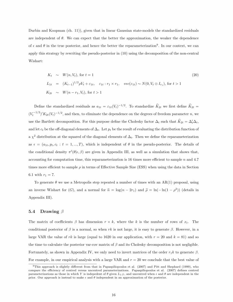
all h. This is confirmed by the impulse response functions in Figure 3, where we can see that ξmon has
the expected impact on GDP growth (GDP) and the 10 year bond yield (BOND), but only through
the homoscedastic component. In contrast, Figure 3 also shows that GDP responds positively to a
shock to SP14 only through its heteroscedastic component (yhett ). Interestingly, a shock to SP affects
both the hetero and homo components of BOND, but with different signs, with the homo component
increasing and the hetero decreasing when SP increases. The negative impact could be interpreted as
the substitution effect between bonds and stocks in the highly volatile and heteroscedastic stock market,
whereas the positive effect can be interpreted through the positive impact that the stock market has
on real economic activity, and therefore on the interest rates.
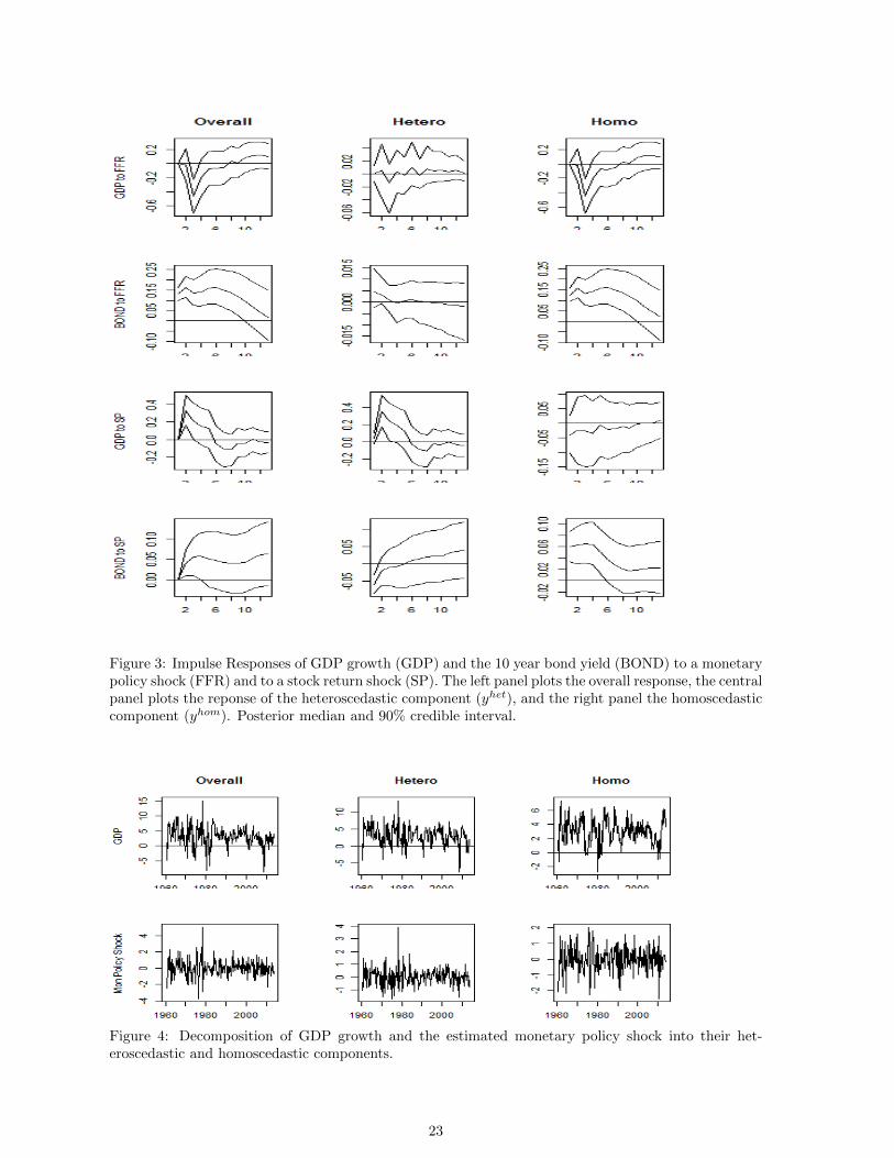
Figure 4 plots the actual value of GDP growth (GDP), and its hetero (GDPhet) and homo (GDPhom)
components, showing what the economy would be if there were only hetero (u1t) or homoscedastic shocks
(u2t). Although both GDPhet and GDPhom have approximately the same average of 3%, we can see
that GDPhom has a smaller variance and becomes negative less often than GDPhet, indicating that an
economy with only homoscedastic shocks would have higher welfare than one with only heteroscedastic
shocks. Figure 4 also decomposes the structural monetary policy shock into the hetero and homo
components, indicating that the hetero component became important in the early 1980s recession,
which is when the FED raised significantly the interest rate following concerns on inflation. Overall,
however, a variance decomposition shows that the structural monetary policy shock is homoscedastic,
with only 3% of its variance caused by the heteroscedastic shocks u1t.
Finally, Figure 5 plots the squared residuals (e2t ), the squared heteroscedastic residuals ((ehett )2) and
the squared homoscedastic residuals ((ehomt )2) for GDP and inflation (INF)15. We can see that the large
spikes in the crises periods are captured only by (ehett )2, whereas (ehomt )2 does not have any noticeable
abnormal behavior during the crises years.
13For the other variables that do not change position with the ordering, the estimated volatilies are the same underboth orderings. The non-diagonal elements are assumed to remain constant with time as in Carriero et al (2015).
14The response to the SP shock is identified by assuming that SP is the fastest variable.15Recall that Section 3 defined ehett = H1et, and ehomt = H2et, where H1 = U1U ′1 and H2 = U2U ′2 = Ir −H1
19
Variable Transformation SpeedReal gross domestic product 400 ∆ log SlowConsumer price index 400 ∆ log SlowEffective Federal funds rate no transformationM2 money stock 400 ∆ log FastPersonal income 400 ∆ log SlowReal personal consumption expenditure 400 ∆ log SlowIndustrial production index 400 ∆ log SlowCivilian unemployment rate no transformation SlowHousing starts log SlowProducer price index 400 ∆ log SlowPersonal consumption expenditures: chain-type price index 400 ∆ log SlowAverage hourly earnings: manufacturing 400 ∆ log SlowM1 money stock 400 ∆ log Fast10-Year Treasury constant maturity rate no transformation FastReal gross private domestic investment 400 ∆ log SlowAll employees: total nonfarm 400 ∆ log SlowISM manufacturing: PMI composite index no transformation SlowISM manufacturing: new orders index no transformation SlowBusiness sector: real output per hour of all Persons 400 ∆ log SlowReal stock prices (S&P 500 index divided by PCE index) 100 ∆ log Fast
Table 1: Definition of Macroeconomic variables in the large VAR and block identification assumption.Fast variables are assumed to react contemporaneously to a shock to the funds rate, whereas slowvariables react only after a lag.
Table 2: Model selection criteria for each value of r1, with n estimated subject to n > 2r1 (Macro data).p(θ) and l(Y |θ) denote the values of the log prior and log likelihood at the posterior mean, respectively.l(Y ) is the approximated marginal likelihood, Pred Lik is the predictive likelihood for observations 51to 214, and Pred BIC is the BIC approximation to the predictive likelihood (calculated as the differencebetween the BIC with the full sample and the BIC with an initial sample). Numerical standard errors(NSE) for the log likelihood values were estimated using 100 independent replications of the particlefilter, with N = Tr1 particles. In all cases, the NSE values were smaller than 0.9.
Table 3: Variance Decompositions. Percentage of var(yt|yt−h), var(yhett |yt−h) and var(yhomt |yt−h)caused by the monetary policy shock (ξt, left panel) and by the heteroscedastic shocks (u1t, rightpanel), for h = 1, 2, 3, 4, 5,∞.
Figure 1: Trace plot and autocorrelations for the (7,7) element of K107, the 4th diagonal element of ρ,for n and the (1,1) element of G (Macro data).
21
Figure 2: Estimated reduced form volatilities and squared Bayesian residuals for the real GDP growthrate (GDP) and the real stock returns (SP). The left panel corresponds to the method of Carriero et al.(2016) under two different orderings: the solid line is for ordering 1 and the dotted line is for ordering2. The central panel corresponds to our method with r1 = 7, and the right panel are the squared of theBayesian residuals.
22
Figure 3: Impulse Responses of GDP growth (GDP) and the 10 year bond yield (BOND) to a monetarypolicy shock (FFR) and to a stock return shock (SP). The left panel plots the overall response, the centralpanel plots the reponse of the heteroscedastic component (yhet), and the right panel the homoscedasticcomponent (yhom). Posterior median and 90% credible interval.
Figure 4: Decomposition of GDP growth and the estimated monetary policy shock into their het-eroscedastic and homoscedastic components.
23
Figure 5: Plot of squared residuals e2t , squared heteroscedastic residuals (ehett )2 and squared homoscedas-tic residuals (ehomt )2 for GDP growth (GDP) and the inflation rate (INF).
6.2 Exchange Rates Data
We use data on 1043 daily returns of 5 exchange rates (AUD, CAD, EUR, JPY, SWF) with respect
to the US dollar, beginning in January 2007 and ending in December 2010 (same data as in Chan et
al. (2018)). Table 4 shows model selection criteria for models under the restriction n > 2r1, and all
indicate that the best model is r1 = 5. Models under the restriction n = r1 + 2 also suggested r1 = 5,
but had worse predictive likelihoods for observations t = 501 −1043. Therefore we can conclude that
these 5 exchange rates are not co-heteroscedastic. Figure 6 shows the posterior volatility estimates and
the squared Bayesian residuals, where we can see that the exchange rates have idiosyncratic spikes,
reinforcing the impression that they do not share heteroscedastic shocks. Figure 7 shows the trace
plots and autocorrelation functions for r1 = 4, indicating that autocorrelations vanish within 10 lags
for most parameters (40 lags for ρ), and the mixing and convergence of the algorithm is good, taking
about 2.8 hours to obtain 15000 iterations with 60 particles. The evaluation of the loglikelihood, using
the average of 100 independent replications of the particle filter, each one with Tr1 = 4172 particles,
took 5.4 minutes, with a numerical standard error of 0.7.
However, the autocorrelations for the model r1 = 5 were much more persistent, with the most
persistent correlations being that of the (1,1) elements of ρ and K = (K1 + ...+KT )/T , which become
smaller than 10% only after 310 and 375 lags, respectively. Even in this case the MCSE values of ρ and
K were only about 8% of the posterior standard deviation, using 15000 iterations with 50 particles,
repeating the sampling of L1:T 30 times within each iteration, and using about 14 hours of computation
time. Appendix II presents more details of how the number of particles affect the effective sample size of
Kt. The evaluation of the loglikelihood for r1 = 5 took about 11.3 minutes, with a numerical standard
Table 4: Model selection criteria for each value of r1, with n estimated subject to n > 2r1 (exchangerates data). Pred Lik is the predictive likelihood for observations 501 to 1043. Column labels as definedin Table 2.
Figure 6: Posterior volatility estimates and squared Bayesian residuals for the returns of five exchangerates: AUD, CAD, EUR, JPY, SWF.
Figure 7: Trace plot and autocorrelations for the (4,4) element of K521, the 4th diagonal element of ρ,n and the (1,1) element of G (exchange rate data) (r1 = 4).
25
7 Concluding remarks
In this paper we have developed methods for Bayesian inference in an inverted Wishart process for
Stochastic Volatility. Unlike most of the previous literature, the model is invariant to the ordering of
the variables and allows for fat tails and the non-existence of higher moments. We provide a novel
algorithm for posterior simulation which uses a pseudo posterior to define a more efficient particle filter,
and to obtain a reparameterization that we find improves computational efficiency.
The modelling framework allows us to determine whether a set of variables share heteroscedastic
shocks and are therefore co-heteroscedastic. Furthermore, the framework allows us to obtain new
variance decompositions as well as new insights on the characteristics of the structural shock and its
impact on the variables of interest. We find strong evidence of co-heteroscedasticity in an application
to a large VAR of 20 macroeconomic variables, and provided a detailed analysis of how monetary policy
and the stock market impact the heteroscedasticity of macroeconomic variables. We also illustrated the
methodology using data on exchange rates, but found no evidence of co-heteroscedasticity.
Future research could look into the implications of co-heteroscedasticity for finding portfolio alloca-
tions with smaller risk and for decision making. Another possible venue is to find ways to reduce the
number of free parameters in G through, for example, the use of Wishart graphical models (e.g. Dawid
and Lauritzen (1993), Wang and West (2009)).
References
Andrieu, C., N.D. Freitas, A. Doucet and M.I. Jordan ”An Introduction to MCMC for Machine Learn-
ing” Machine Learning, 50, 5–43.
Andrieu, C., A. Doucet, and R. Holenstein, (2010), ”Particle Markov chain Monte Carlo methods,”
Journal of the Royal Statistical Society: Series B (Statistical Methodology), 72, 269–342.
Anderson T.W. and Girshick, M.A. (1944) ”Some Extensions of the Wishart Distribution,” The Annals
of Mathematical Statistics, 15, 345-357.
Asai, M. and M. McAleer (2009) ”The Structure of Dynamic Correlations in Multivariate Stochastic
Volatility Models,” Journal of Econometrics, 150, 182-192.
Banbura, B., D. Giannone and L. Reichlin, (2010) ”Large Bayesian vector auto regressions,” Journal
of Applied Econometrics, 25, 71-92.
Bauwens, L., M. Lubrano, and J.F. Richard (1999) Bayesian Inference in Dynamic Econometric Models.
Oxford: Oxford University Press.
26
Bollerslev, T. (1986) ”Generalized Autoregressive Conditional Heteroskedasticity,” Journal of Econo-
metrics, 31, 307-327.
Carriero, A., Clark, T.E. and Marcellino, M. (2015) ”Large vector autoregressions with asymmetric
priors and time varying volatilities,” Working Paper No. 759, School of Economics and Finance,
Queen Mary University of London.
Casarin, R. and D. Sartore, (2007), ”Matrix-state particle filters for Wishart stochastic volatility
processes,” in Proceedings SIS, 2007 Intermediate Conference, Risk and Prediction, 399-409, CLEUP
Padova.
Chan, J. (2013) ” Moving average stochastic volatility models with application to inflation forecast,”
Journal of Econometrics, 176, 162-172
Chan, J. (2018) ”Large Bayesian VARs: A Flexible Kronecker Error Covariance Structure,” Journal of
Business & Economic Statistics DOI: 10.1080/07350015.2018.1451336
Chan, J., R. Leon-Gonzalez, and R. Strachan (2018) ”Invariant Inference and Efficient Computation in
the Static Factor Model,” Journal of the American Statistical Association, 113, 819-828.
Chib, S., I. Jeliazkov (2001) ”Marginal Likelihood From the Metropolis–Hastings Output,” Journal of
the American Statistical Association, 96, 270-281.
Chiu, C.W., H. Mumtaz, and G. Pinter (2017) “Forecasting with VAR models: Fat tails and stochastic
volatility,” International Journal of Forecasting, 33, 1124-1143
Clark, T.E. and F. Ravazzolo (2015), ”Macroeconomic Forecasting Performance Under Alternative
Specifications of Time-Varying Volatility,” Journal of Applied Econometrics, 30, 551–575.
Dawid, A.P. and S.L. Lauritzen (1993) ”Hyper-Markov laws in the statistical analysis of decomposable
graphical models,” The Annals of Statistics, 3, 1272-1317.
Durbin, J. and S.J. Koopman (2001) Time Series Analysis by State Space Methods, Oxford University
Press.
Engle, R. (1982) ”Autoregressive Conditional Heteroscedasticity with Estimates of the Variance of
United Kingdom Inflation” Econometrica, 50, 987-1007.
Flegal, J.M., M. Haran and G.L. Jones, (2008). Markov Chain Monte Carlo: Can We Trust the Third
Note that the process Zt = Zt−1ρ + εt with Z1 following the stationary distribution can be equiv-
31
alently written as Zt−1 = Ztρ + εt with ZT following the stationary distribution16. Therefore we can
apply the same decomposition to the reverse process as follows:
L1,t−1 =−→Z ′tZt−1 =
(−→Z t
)′Zt︸ ︷︷ ︸
K1/2t
ρ+(−→Z t
)′εt︸ ︷︷ ︸
ε1t
(25)
L2,t−1 =−→Z ′t⊥Zt−1 =
(−→Z t⊥
)′Ztρ︸ ︷︷ ︸
0
+(−→Z t⊥
)′εt =
(−→Z t−1,⊥
)′εt︸ ︷︷ ︸
ε2t
K2t = L′2tL2t
Note that L1t =−→Z ′t−1Zt = (K
−1/2t−1 )′Z ′t−1Zt, while L1,t−1 =
−→Z ′tZt−1 = (K
−1/2t )′Z ′tZt−1, and
therefore we can conclude that Z ′tZt−1 = (K1/2t )′L1,t−1 = ((K
1/2t−1)′L1t)
′, from where we can arrive at
(15) and the inverse transformation (19).
The algorithm to generate a value for L1:T in reverse order is analogous to the natural order algorithm
in Section 5.1. Let Lt = (L1t, K2t) for t < T, LT = KT , and L1:T = (L1, L2, ..., LT ). Let the N particles
be denoted as Lkt = (Lk1t, Kk2t) for t < T and LkT = (Kk
T ). Define Kkt = (Lk1t)
′Lk1t+ Kk2t for t < T . Given
the definition of Vt in (17), the value of L1:T at iteration i, denoted as L1:T (i) = (L1(i), ..., LT (i)), can
be generated given the previous value L1:T (i− 1) as follows:
Algorithm 4 Reverse order cPFBS.
Step 1: Fix the last particle equal to L1:T (i− 1), that is, LN1:T = L1:T (i− 1)
Step 2: at time t = T ,
(a) sample KkT ∼Wr1(n, VT ) for k = 1, ..., N − 1, and
(b) compute and normalize the weights:
wkT :=∣∣Kk
T
∣∣0.5 , W kT := wkT /(
N∑m=1
wmT ), k = 1, ..., N
Step 3: at times t = T − 1, ..., 1,
(a) sample the indices Akt+1, for k = 1, ..., N − 1, from a multinomial distribution on (1, ..., N) with
probabilities Wt+1 = (W 1t+1, ...,W
Nt+1)
16This can easily be proved from Zt = Zt−1ρ + εt by writing (Z1, ..., ZT ) as a vector Z =(vec(Z1)′, vec(Z2)′, ..., vec(ZT )′)′, and noting that the joint distribution of Z is normal with 0 mean and covarianceV :
V =
(I − ρ2)−1 ⊗ In (I − ρ2)−1ρ⊗ In ... (I − ρ2)−1ρT−1 ⊗ Inρ′(I − ρ2)−1 ⊗ In (I − ρ2)−1 ⊗ In (I − ρ2)−1ρT−2 ⊗ In
ρ(T−1)′(I − ρ2)−1 ⊗ In ρ(T−2)′(I − ρ2)−1 ⊗ In (I − ρ2)−1 ⊗ In
and also the distribution of Z = (vec(ZT )′, vec(ZT−1)′, ..., vec(Z1)′)′ is normal with the same 0 mean and covariancematrix V , and so we can also write Zt = Zt+1ρ+ εt provided ZT comes from the stationary distribution.
32
(b) sample vec(Lk1t) ∼ N(
(KAkt+1
t+1
)1/2
ρVt, Ir1 ⊗ Vt) and Kk2t ∼ Wr1(n − r1, Vt), calculate Kk
t =
(Lk1t)′Lk1t + Kk
2t for k = 1, ..., N − 1 and
(c) compute and normalize the weights
wkt :=∣∣Kk
t
∣∣0.5 , W kt := wkt /(
N∑m=1
wmt ), k = 1, ..., N
Step 4: at time t = 1, sample b1 from a multinomial distribution on (1, ..., N) with probabilities W1,
and set L1(i) = Lb11 .
Step 5: at times t = 2, ..., T
(a) compute the updated weights
wkt = wkt f(Kbt−1
t−1 |Kkt ),..., W k
t := wkt /(
N∑m=1
wmt ), k = 1, ..., N , where
µkt = (Kkt )1/2ρVt−1, f(K
bt−1
t−1 |Kkt ) = exp(−1
2tr(V −1t−1(L
bt−1
1(t−1) − µkt )′(L
bt−1
1(t−1) − µkt ))
(b) sample bt from a multinomial distribution on (1, ..., N) with probabilities Wt = (W 1t , ..., W
Nt ),
and set Lt(i) = Lbtt .
In order to see the impact of alternating the order, we fix (G, β) equal to their posterior means
and (n, ρ) equal to their posterior medians and calculate the Effective Sample Size (ESS) of the (1,1)
element of Kt for 10000 iterations using the Macro data with r1 = 7 (Table 5) and the Exchange Rate
Data with r1 equal to 4 and 5 (Table 6). The ESS values are not adjusted by computing time because
the differences in computing time among algorithms are negligible. We can see that the ESS values of
KT are always bigger (smaller) than the ESS values of K1 in the natural order (reverse order) algorithm,
respectively. The alternating order algorithm has always better ESS than the natural order for K1, and
better ESS than the reverse order for KT . The gains imply that ESS is increased at least by a factor
of 3 (with Exchange rate data, 95 particles and r1 = 4) and at most by a factor of 260 (with Exchange
rates data, 95 particles and r1 = 5). However, the alternating order algorithm has lower ESS than
the natural order for KT , and lower ESS than the reverse order for K1, but the factor of increase of
the single order algorithms over the alternating algorithm is only between 1.4 and 2.9. Looking at the
ESS of KT/2 (i.e. at the middle of the sample), the alternating order algorithm has always better ESS
when using the Macro data (Table 5), with the factor of improvement ranging between 1.01 (with 110
particles) and 1.55 (with 25 particles). With the exchange rates data the alternating order algorithm is
always better than the natural order to sample KT/2, but the reverse order algorithm is even better in
5 out of 8 cases. To get a measure of which algorithm is overall better to sample K1:T , we calculate the
Table 5: Effective sample size of K with 10000 iterations and r1 = 7 using the Macro data. The columnwith label ’order’ takes values (-1,0,1) for reverse, alternating and natural order, respectively. N is thenumber of particles and the columns (K1, KT/2, KT ,K) give the Effective Sample Size (ESS) with 10000
iterations of sampling the (1,1) element of (K1, KT/2, KT ,K), where K = (K1 + ...+KT )/T . The two
columns under ’Gain (%)’ give the percentage increase in the ESS of the (1,1) element of K when usingalternating order with respect to reverse order (left) and natural order (right). The parameters (G, β)were fixed equal to their posterior means and (n, ρ) equal to their posterior medians.
ESS of K = (K1 + ...+KT )/T . We find that the alternating order algorithm is the best in all but one
case, increasing the ESS by at most 140% and at least by 1%. The only exception is with the exchange
rate data with r1 = 5 and 95 particles, where the ESS of the reverse order algorithm is 42% better.
Overall we can conclude that the ordering in sampling K1:T affects the efficiency of the algorithm, and
that for our datasets alternating the ordering brings almost always computational gains.
Appendix III
This appendix is for Section 5.3 and it gives details on the reparameterization function ε = fθ(L1:T ),
its inverse f−1θ (ε), the density πt(θ|ε, β), and a simulation to illustrate the better performance of the
reparameterization.
Defining ε = (a2:T , p1:T , c1:T ), the following algorithm can be used to calculate ε = fθ(L1:T ).
Algorithm 5 To obtain ε = fθ(L1:T ).
Step 1: at time t = 1,
(a) Define K1 = (V−1/21 )′K1(V
−1/21 ), and ∆1 as an upper triangular matrix such that K1 = ∆′1∆1,
with c1 being the off-diagonal elements of ∆1.
(b) Let d1 = (d11, d21, ..., dr11) be the diagonal elements of ∆1. Let p1 = (p11, p21, ..., pr11), with
pi1 = Fχ2(fni1)(d2i1), where Fχ2(fni1)
(d2i1) is the distribution function of a chi-squared with fni1 = n+ i+ 1
degrees of freedom.
Step 2: at times t = 2, ..., T ,
34
r1 N order K1 KT/2 KT K Gain (%)-1 4755 1277 436 127
Table 6: Effective sample size of K with 10000 iterations and r1 = 4 and 5, using the Exchange Ratedata. Column labels have the same meaning as in Table 5. The parameters (G, β) were fixed equal totheir posterior means and (n, ρ) equal to their posterios medians.
35
(a) Calculate at as:
at = (L1t − (Kt−1)1/2ρVt)V−1/2t , for t > 1
(b) Calculate K2t = (V−1/2t )′K2t(V
−1/2t ), and ∆t as an upper triangular matrix such that K2t =
∆′t∆t, with ct being the off-diagonal elements of ∆t.
(c) Let dt = (d1t, d2t, ..., dr1t) be the diagonal elements of ∆t. Let pt = (p1t, p2t, ..., pr1t), with
pit = Fχ2(fnit)(d2it), where Fχ2(fnit)
(d2it) is the distribution function of a chi-squared with fnit = n−r1+i+1
degrees of freedom.
The inverse transformation is denoted as Lθ∗1:T = f−1θ∗ (ε), for θ∗ = (G∗, ρ∗, n∗), where we write Lθ∗1:T
instead of L1:T to make clear that for a fixed value of ε, L1:T changes when θ changes. For this reason we
also use the notation (Kθt ,K
θ2t, L
θ1t, V
θt ) for (Kt,K2t, L1t, Vt) below. The following algorithm describes
how to obtain Lθ∗1:T = f−1θ∗ (ε).
Algorithm 6 To obtain Lθ∗1:T = f−1θ∗ (ε)
Step 1: Calculate (V θ∗
1 , V θ∗
2 , ..., V θ∗
T ) using the recursion in (11) and the value of θ∗ = (G∗, ρ∗, n∗).
Step 2: at time t = 1
(a) Obtain the vector dn∗
t = (dn∗
1t , dn∗
2t , ..., dn∗
r1t), by calculating dn∗
it =(F−1χ2(fn
∗it )
(pit))1/2
, where
F−1χ2(fn
∗it )
is the inverse of the distribution function of a chi-squared with fn∗
it = n∗ + i + 1 degrees
of freedom.
(b) Construct ∆θ∗
t as an upper triangular matrix with off diagonal elements equal to ct and diagonal
equal to dn∗
it .
(c) Calculate Kθ∗
1 =((V θ
∗
t )1/2)′ (
∆θ∗
t
)′∆θ∗
t (V θ∗
t )1/2
Step 3: at times t = 2, ..., T
(a) Calculate
Lθ∗
1t = (Kθ∗
t−1)1/2ρ∗V θ∗
t + at(Vθ∗
t )1/2
(b) Obtain the vector dn∗
t = (dn∗
1t , dn∗
2t , ..., dn∗
r1t), by calculating dn∗
it =(F−1χ2(fn
∗it )
(pit))1/2
, where
F−1χ2(fn
∗it )
is the inverse of the distribution function of a chi-squared with fn∗
it = n∗ − r1 + i + 1 de-
grees of freedom.
(c) Construct ∆θ∗
t as an upper triangular matrix with off diagonal elements equal to ct and with
diagonal equal to dn∗
t
(d) Calculate Kθ∗
2t =((V θ
∗
t )1/2)′ (
∆θ∗
t
)′∆θ∗
t (V θ∗
t )1/2.
The following proposition gives the conditional posterior density of θ given (ε, β).
36
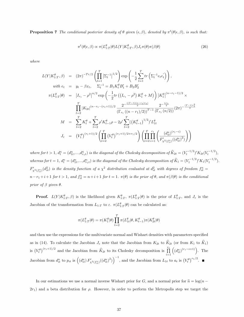
Proposition 7 The conditional posterior density of θ given (ε, β), denoted by πt(θ|ε, β), is such that:
where for t > 1, dnt = (dn1t,...,dnr1t) is the diagonal of the Cholesky decomposition of K2t = (V
−1/2t )′K2t(V
−1/2t ),
whereas for t = 1, dnt = (dn1t,...,dnr1t) is the diagonal of the Cholesky decomposition of K1 = (V
−1/21 )′K1(V
−1/21 ).
F ′χ2(fnit)(d2it) is the density function of a χ2 distribution evaluated at d2it with degrees of freedom fnit =
n−r1 + i+1 for t > 1, and fnit = n+ i+1 for t = 1. π(θ) is the prior of θ, and π(β|θ) is the conditional
prior of β given θ.
Proof. L(Y |Kθ1:T , β) is the likelihood given Kθ
1:T , π(Lθ1:T |θ) is the prior of Lθ1:T , and Jε is the
Jacobian of the transformation from L1:T to ε. π(Lθ1:T |θ) can be calculated as:
π(Lθ1:T |θ) = π(Kθ1 |θ)
T∏t=2
π(Lθ1t|θ,Kθt−1)π(Kθ
2t|θ)
and then use the expressions for the multivariate normal and Wishart densities with parameters specified
as in (14). To calculate the Jacobian Jε note that the Jacobian from K2t to K2t (or from K1 to K1)
is(V θt)(r1+1)/2
and the Jacobian from K2t to its Cholesky decomposition isr1∏i=1
((dnit)
(r1−i+1))
. The
Jacobian from dnit to pit is(
(dnit)F′χ2(fnit)
((dnit)2))−1
, and the Jacobian from L1t to at is(V θt)r1/2
.
In our estimations we use a normal inverse Wishart prior for G, and a normal prior for n = log(n−
2r1) and a beta distribution for ρ. However, in order to perform the Metropolis step we target the
37
conditional posterior of (G, n, ρ), where ρ = ln(− ln(1− ρ2)). The prior for π(ρ) can be obtained as:
π(ρ) = π(ρ)Jρ
Jρ =1− ρ2
2ρ(− ln(1− ρ2))
where Jρ is the Jacobian. As a proposal density we use an inverse Wishart for G centered at ((1 −
τG)G(i− 1) + τGG), where G(i− 1) is the value of G in the previous iteration and G is a preliminary
estimate of G. For % = (n, ρ) we use a normal proposal density centered at ((1 − τρ)%(i − 1) + τρ%),
where % is a preliminary estimate and %(i− 1) is the value of % in the previous iteration.
Figure 8 shows the trace plot and autocorrelations when no reparameterization is used, using the
macro data of Section 6.1. We can see that the autocorrelations are much more persistent than those
in Figure 1, particularly for ρ and n. For example, the lag 40 autocorrelation of n (ρ) is 0.87 (0.69)
with no reparameterization, but equal to 0.01 (0.025) with the reparameterization, respectively. The
effective sample sizes (ESS) of 10000 after burn-in iterations for (K, ρ, n, G) are (439, 81, 24, 107),
without reparameterization and equal to (960, 878, 877, 522) with the reparameterization. However,
the computation time with the latter is about 2.3 higher. Therefore, taking into account computation
time, the algorithm with the reparameterization is about 16 times more efficient to sample n, 4.7 times
more efficient to sample ρ, 2.3 times more efficient to sample G and roughly equally efficient to sample
K.
Figure 8: Trace plot and autocorrelations when no reparameterization is used in the model with r1 = 7(Macro data). Trace plots and autocorrelations are for the (7,7) element of KT/2, the 4th diagonalelement of ρ, for n and the (1,1) element of G.
Appendix IV
This appendix gives the details of the conditional prior and posterior of β, discussed in Section 5.4.
38
Proposition 8 Assuming that the conditional prior of vec(β′)|G is a normal with mean µβ and co-
variance matrix V β given by:
V β = (G⊗ V 0) , for V 0 : k × k
the conditional posterior vec(β′)|G,K1:T is also normal with mean µβ and covariance matrix V β given
by:
V β = (A1 ⊗ Ik)
(T∑t=1
(Kt ⊗ xtx′
t) + I−1r1 ⊗ V−10
)−1(A′1 ⊗ Ik) + (27)A2A
′2 ⊗
(T∑t=1
(xtx′
t) + V −10
)−1µβ = V β
(vec(
T∑t=1
xty′tΣ−1t ) +
(G−1 ⊗ V −10
)µβ
)(28)
with I−1r1 = (n− r1 − 1)(Ir1 − ρ2)−1
A draw of vec(β′)|G,K1:T can be obtained as((V β)1/2)′
η+µβ where η is a rk×1 vector of independent
standard normal variates, and(V β)1/2
can be calculated as:
(V β)1/2
= (D1, D2)′, D1 : rk × r1k, D2 : rk × r2k (29)
D1 = (A1 ⊗ Ik)
( T∑t=1
(Kt ⊗ xtx′
t) + I−1r1 ⊗ V−10
)−1/2′
D2 = A2 ⊗
( T∑t=1
(xtx′
t) + V −10
)−1/2′
Proof. Standard calculations, similar to those in a multivariate regression model, show that V β is
given by
V β =
(T∑t=1
(Σ−1t ⊗ xtx′t
)+G−1 ⊗ V −10
)−1(30)
and that µβ is given by (28). However, expression (30) requires the inversion of a rk × rk matrix. To
obtain (27) first note that (3) and (22) imply that
G−1 = B
I−1r1 0
0 Ir2
B′, Σ−1t = B
Kt 0
0 Ir2
B′
39
Hence we can write (30) as:
V β =
(B ⊗ Ik)
T∑t=1
Kt 0
0 Ir2
⊗ xtx′t+
I−1r1 0
0 Ir2
⊗ V −10
(B′ ⊗ Ik)
−1
V β = (A⊗ Ik)
∑T
t=1Kt ⊗ xtx′t + I−1r1 ⊗ V−10 0
0 Ir2 ⊗(∑T
t=1 xtx′t + V −10
)−1
(A′ ⊗ Ik)
V β = (A1 ⊗ Ik)
(T∑t=1
(Kt ⊗ xtx′t) + I−1r1 ⊗ V−10
)−1(A′1 ⊗ Ik) +A2A
′2 ⊗
(T∑t=1
xtx′t + V −10
)−1(31)
which is equal to (27), and where we have used that A ⊗ Ik = (A1, A2) ⊗ Ik = (A1 ⊗ Ik, A2 ⊗ Ik). To


![Abstract arXiv:1509.05084v2 [math.NA] 24 Sep 2016 · An Accelerated Dual Proximal Gradient Method for Applications in Viscoplasticity Timm Treskatisa,1,, Miguel A. Moyers-Gonz alez](https://static.documents.pub/doc/80x56/5b5f168f7f8b9a8b4a8d9aa4/abstract-arxiv150905084v2-mathna-24-sep-2016-an-accelerated-dual-proximal.jpg)


