Journal of American Science 2013;9(2) http://www.jofamericanscience.org http://www.jofamericanscience.org [email protected]22 Development of a Unified Model for Prediction of Asphaltene Deposition Profile along Wellbore Saeid Dowlati, Mohammad Jamialahmadi Department of Petroleum Engineering, Petroleum University of Technology, Ahwaz, Iran [email protected]Abstract: Asphaltene deposition is one of major production problems during life of an oil well. This phenomenon results in reduction of well flow rate or total blockage of wellbore. Prediction of asphaltene deposition along wellbore can identify most-probable region of deposition and investigate effect of different parameters on deposition profile. In this work a comprehensive model to predict asphaltene deposition profile along wellbore is developed. The wellbore is discretized into some grids, and pressure, temperature, and asphaltene concentration at each grid is calculated using well known models. Then these data are used to predict asphaltene deposition profile. The unified model is applied to a southwestern Iranian wellbore. Effect of deposition on wellbore modeling investigated and it is shown that deposition profile must be considered to update wellbore diameter during production. Effect of flow velocity on deposition profile also examined and it is shown that increasing velocity how can reduce asphaltene deposition rate. [Saeid Dowlati, Mohammad Jamialahmadi. Development of a Unified Model for Prediction of Asphaltene Deposition Profile along Wellbore. J Am Sci 2013;9(2):22-31]. (ISSN: 1545-1003). http://www.jofamericanscience.org . 4 Keywords: asphaltene deposition, wellbore unloading, hydrodynamic modeling, deposition profile 1. Introduction Crude oil is considered as a colloidal mixture consisting of four major groups namely saturated hydrocarbons, aromatics, resins and asphaltenes (Mullins et al., 2007). Asphaltene is viewed as the most polar and highest molecular weight fraction of the crude oil (Yen et al, 1961). Asphaltene are generally defined as the fraction that is soluble in aromatics solvent such as benzene or toluene, and insoluble in normal alkanes such as n-pentane or n-heptane (Speight, 2006). Asphaltenes are stabilized in oil by means of the resin molecules, which act as peptizing agent to emulsify asphaltene particles (Bunger and Li, 1982). Colloidal asphaltene particles may be naturally or artificially precipitated from oil, if the resin molecules are removed from the surface of asphaltene particles (Jamialahmadi et al., 2009). Asphaltenes and resins are in the thermodynamic equilibrium at static reservoir condition. However, changes in thermodynamic condition such as pressure, temperature or compositions during oil production may render asphaltene unstable and precipitate from crude oil and could deposit in reservoir, wellbore, wellhead facilities, transporting pipeline and surface processing facilities (Khalil et al., 1997). The main change of pressure and temperature of crude oil during production process is along well string, so the most probable region to face asphaltene deposition problem is wellbore (Soltani et al., 2009). Asphaltene deposition results in reduction of available wellbore diameter to flow, and consequently reduction of wellhead pressure or flow rate, based on production scenario. Severe pressure drop along wellbore and unloading of well are consequences of resumption of asphaltene deposition. This problem cause cease of production and necessity for work-over operation, which impose a huge expenditure on production project. Therefore modeling of asphaltene deposition profile along the wellbore is the first and main step in reduction and control of this problem. Reliable modeling of this phenomenon results in prediction of most probable section of wellbore to deposition problem, investigate effect of tubing size on problem, and selection of optimum wellhead pressure and flow rate to minimize deposition problem. Several authors have investigated thermodynamic behavior of asphaltene particles in crude oils. A vast number of asphaltene precipitation models have been developed through these investigations. These models focus on solubility behavior of asphaltene particles, and unfavorable conditions which result in asphaltene particles come out of solution. Among them some noteworthy works have been published during past few decades (Hirschberg et al., 1984; Kawanka et al., 1991; Rassamdana et al., 1996; Mansoori, 1999; Nghiem, 1999; Browarzik et al., 1999) Prediction of asphaltene precipitation is not sufficient for modeling asphaltene deposition profile. The key point in developing such model is prediction of asphaltene deposition rate. A few works have been done on developing a reliable model to predict rate of asphaltene deposition from operational parameters. Among them Jamialahmadi et al. (2009) developed a reliable mechanistic model for prediction of
Transcript
Journal of American Science 2013;9(2) http://www.jofamericanscience.org
Development of a Unified Model for Prediction of Asphaltene Deposition Profile along Wellbore
Saeid Dowlati, Mohammad Jamialahmadi
Department of Petroleum Engineering, Petroleum University of Technology, Ahwaz, Iran [email protected]
Abstract: Asphaltene deposition is one of major production problems during life of an oil well. This phenomenon results in reduction of well flow rate or total blockage of wellbore. Prediction of asphaltene deposition along wellbore can identify most-probable region of deposition and investigate effect of different parameters on deposition profile. In this work a comprehensive model to predict asphaltene deposition profile along wellbore is developed. The wellbore is discretized into some grids, and pressure, temperature, and asphaltene concentration at each grid is calculated using well known models. Then these data are used to predict asphaltene deposition profile. The unified model is applied to a southwestern Iranian wellbore. Effect of deposition on wellbore modeling investigated and it is shown that deposition profile must be considered to update wellbore diameter during production. Effect of flow velocity on deposition profile also examined and it is shown that increasing velocity how can reduce asphaltene deposition rate. [Saeid Dowlati, Mohammad Jamialahmadi. Development of a Unified Model for Prediction of Asphaltene Deposition Profile along Wellbore. J Am Sci 2013;9(2):22-31]. (ISSN: 1545-1003). http://www.jofamericanscience.org. 4 Keywords: asphaltene deposition, wellbore unloading, hydrodynamic modeling, deposition profile 1. Introduction
Crude oil is considered as a colloidal mixture consisting of four major groups namely saturated hydrocarbons, aromatics, resins and asphaltenes (Mullins et al., 2007). Asphaltene is viewed as the most polar and highest molecular weight fraction of the crude oil (Yen et al, 1961).
Asphaltene are generally defined as the fraction that is soluble in aromatics solvent such as benzene or toluene, and insoluble in normal alkanes such as n-pentane or n-heptane (Speight, 2006). Asphaltenes are stabilized in oil by means of the resin molecules, which act as peptizing agent to emulsify asphaltene particles (Bunger and Li, 1982). Colloidal asphaltene particles may be naturally or artificially precipitated from oil, if the resin molecules are removed from the surface of asphaltene particles (Jamialahmadi et al., 2009). Asphaltenes and resins are in the thermodynamic equilibrium at static reservoir condition. However, changes in thermodynamic condition such as pressure, temperature or compositions during oil production may render asphaltene unstable and precipitate from crude oil and could deposit in reservoir, wellbore, wellhead facilities, transporting pipeline and surface processing facilities (Khalil et al., 1997). The main change of pressure and temperature of crude oil during production process is along well string, so the most probable region to face asphaltene deposition problem is wellbore (Soltani et al., 2009). Asphaltene deposition results in reduction of available wellbore diameter to flow, and consequently reduction of wellhead pressure or flow rate, based on production
scenario. Severe pressure drop along wellbore and unloading of well are consequences of resumption of asphaltene deposition. This problem cause cease of production and necessity for work-over operation, which impose a huge expenditure on production project. Therefore modeling of asphaltene deposition profile along the wellbore is the first and main step in reduction and control of this problem. Reliable modeling of this phenomenon results in prediction of most probable section of wellbore to deposition problem, investigate effect of tubing size on problem, and selection of optimum wellhead pressure and flow rate to minimize deposition problem.
Several authors have investigated thermodynamic behavior of asphaltene particles in crude oils. A vast number of asphaltene precipitation models have been developed through these investigations. These models focus on solubility behavior of asphaltene particles, and unfavorable conditions which result in asphaltene particles come out of solution. Among them some noteworthy works have been published during past few decades (Hirschberg et al., 1984; Kawanka et al., 1991; Rassamdana et al., 1996; Mansoori, 1999; Nghiem, 1999; Browarzik et al., 1999)
Prediction of asphaltene precipitation is not sufficient for modeling asphaltene deposition profile. The key point in developing such model is prediction of asphaltene deposition rate. A few works have been done on developing a reliable model to predict rate of asphaltene deposition from operational parameters. Among them Jamialahmadi et al. (2009) developed a reliable mechanistic model for prediction of
Journal of American Science 2013;9(2) http://www.jofamericanscience.org
asphaltene deposition based on a thermal approach. They set up an experimental apparatus which has been used to measure the mass of deposited asphaltene particles as a function of time, via the measurement of the heat transfer coefficient and the thermal resistance of asphaltene deposit. The experimental results in coupling with study and formulation of mechanism of asphaltene deposition process have been used to develop a mechanistic model for prediction of the rate of asphaltene deposition.
Also some authors have published their works recently on developing a thorough model for prediction of asphaltene deposition profile using different approaches (Soltani et al., 2009; Ramirez-Jaramillo et al., 2010; Vargas et al., 2010).
The purpose of current work is to develop a comprehensive simulator to predict asphaltene deposition profile along the wellbore. This approach is based on Jamialahmadi et al. (2009) model to predict deposition profile, and a mechanistic approach to develop thermal and hydrodynamic model of wellbore. 2. Methodology
Prediction of asphaltene deposition profile along wellbore, needs calculation of asphaltene precipitation in wellbore. Asphaltene precipitation prediction needs hydrodynamic and thermal modeling of wellbore. The first step in modeling of asphaltene deposition profile is calculation of pressure and temperature profiles along the wellbore. For hydrodynamic and thermal modeling of wellbore a finite difference approach used to obtain a descriptive condition of a desired well. In this approach wellbore is descritized into a number of grids and flowing model of well is simulated in each grid. Considering the basic assumption of finite difference approach, well conditions assumed constant in each grid. First for each grid an EOS-based model coupled with empirical correlations is used, to achieve all the desired fluid properties. These fluid properties are used to predict pressure and temperature profile along the wellbore. Pressure drop calculations needs fluid temperature to predict fluid properties; in other hand, temperature calculations need two-phase flow parameters, such as liquid hold-up, to obtain a correct temperature at the end of each grid. So hydrodynamic and thermal modeling of wellbore needs an iterative approach to solve both sets of equations conjugatively. So pressure and temperature in each grid can be obtained.
Flash calculations and stability analysis have been done based on Pan and Firoozabadi algorithm (2001) to determine number of phases, bubble point pressure, and composition, z-factor, and density of each existed phase. Also interfacial tension between
two phases has been obtained from Katz and Saltman (1939) equation. Other necessary fluid properties such as Rs, Bo, gas and oil viscosity and fluid compressibility estimated using empirical correlations.
Hydrodynamic modeling of wellbore has been done using a mechanistic model for upward two-phase flow in wellbores. Mechanistic modeling approach has emerged in the early of 80’s and attempts to formulate two-phase flow based on real physical phenomena of flow (Gomez et al., 1999). Ansari et al. (1994) developed their model based on mathematically modeling of two-phase flow. Their model is composed of a model for flow-pattern prediction as bubble, slug, and annular flow. Then a set of independent mechanistic models for prediction of two-phase flow parameters such as pressure gradient and liquid hold-up are used. This model shows great improved performance over empirical two-phase correlations.
Thermal modeling of wellbore is done by using Ramey’s model (1962). This model was developed based on assumption of heat transfer in the wellbore is steady state. Heat resistance in each section of wellbore must be calculated to achieve a reliable temperature profile along wellbore. Also heat transfer coefficient and overall heat transfer coefficient are calculated using Prandtl (1944) and Ramey (1962) equations.
(1)
(2)
Thermal properties of fluids and completion string which used in thermal modeling are listed in Tables (1) and (2).
Table 1. Thermal properties of fluids and completion
Results of above calculations in addition to crude oil properties used to predict asphaltene precipitated content in each grid.
For prediction of asphaltene precipitation Nghiem et al. (1993) used a solid model. In this model the plus fraction is split into two pseudo-
Properties Oil Gas Water Thermal Conductivity
( ) 0.08 0.02 0.336
Specific Heat
( ) 0.45 0.55 1.00
Thermal Diffusivity
( ) ---- ---- ----
Journal of American Science 2013;9(2) http://www.jofamericanscience.org
components: a non-precipitating pseudo-component and a precipitating pseudo-component. These two pseudo-components have the same critical properties and accentric factor, but their interaction coefficients with the light components are different. The precipitating pseudo-component has larger interaction coefficients with the light components. The larger the interaction coefficients, the greater the incompatibility between components. The precipitating pseudo-component is the only component which can comes out of solution and forms a solid phase. Three-phase flash calculations are done to determine the mole fraction of vapor and solid phases. Table 2 - Thermal Properties of Completion String Employed in Simulation
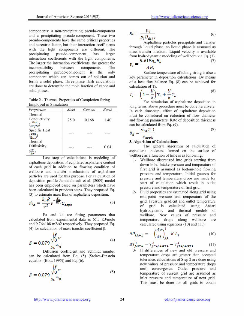
Last step of calculations is modeling of asphaltene deposition. Precipitated asphaltene content of each grid in addition to flowing condition of wellbore and transfer mechanisms of asphaltene particles are used for this purpose. For calculation of deposition profile Jamialahmadi et al. (2009) model has been employed based on parameters which have been calculated in previous steps. They proposed Eq. (3) to estimate mass flux of asphaltene deposition.
(3)
Ea and kd are fitting parameters that
calculated from experimental data as 65.3 KJ/mole and 9.76×10⁸ m2/s2 respectively. They proposed Eq. (4) for calculation of mass transfer coefficient β.
(4)
Diffusion coefficient and Schmidt number can be calculated from Eq. (5) (Stokes-Einstein equation (Bott, 1995)) and Eq. (6).
(5)
(6)
Asphaltene particles precipitate and transfer through liquid phase, so liquid phase is assumed as mass transfer medium. Liquid velocity is available from hydrodynamic modeling of wellbore via Eq. (7).
(7)
Surface temperature of tubing string is also a key parameter in deposition calculations. By means of a heat flux balance Eq. (8) can be achieved for calculation of Ts.
(8)
For simulation of asphaltene deposition in long terms, above procedure must be done iteratively. In each time-step, effect of asphaltene deposition must be considered on reduction of flow diameter and flowing parameters. Rate of deposition thickness can be calculated from Eq. (9).
(9)
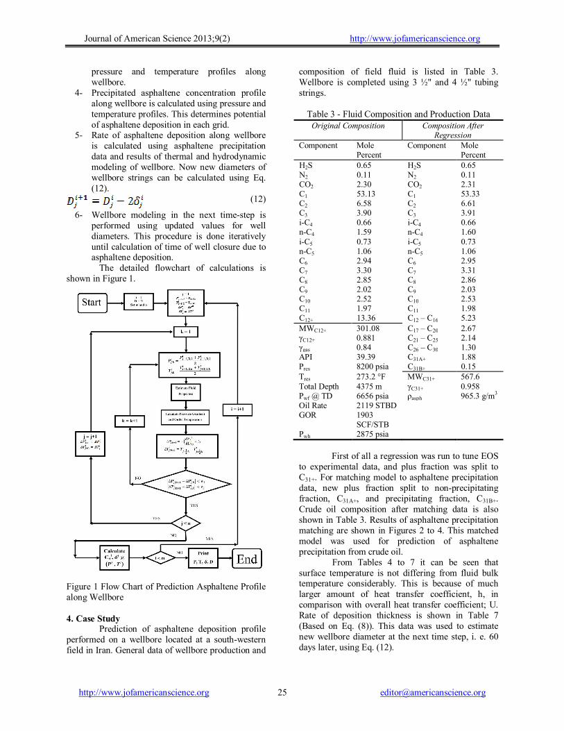
3. Algorithm of Calculations The general algorithm of calculation of
asphaltene thickness formed on the surface of wellbore as a function of time is as following:
1- Wellbore discretized into grids starting from down-hole. Intake pressure and temperature of first grid is assumed as bottom-hole flowing pressure and temperature. Initial guesses for pressure and temperature drops are made for start of calculation which result in outlet pressure and temperature of first grid.
2- Fluid properties are estimated along grid using mid-point pressure and temperature of the grid. Pressure gradient and outlet temperature of grid is calculated using Ansari hydrodynamic and thermal models of wellbore. New values of pressure and temperature drops along wellbore are calculated using equations (10) and (11).
(10)
(11)
3- If differences of new and old pressure and temperature drops are greater than accepted tolerance, calculations of Step 2 are done using new values of pressure and temperature drops until convergence. Outlet pressure and temperature of current grid are assumed as inlet pressure and temperature of next grid. This must be done for all grids to obtain
Journal of American Science 2013;9(2) http://www.jofamericanscience.org
4- Precipitated asphaltene concentration profile along wellbore is calculated using pressure and temperature profiles. This determines potential of asphaltene deposition in each grid.
5- Rate of asphaltene deposition along wellbore is calculated using asphaltene precipitation data and results of thermal and hydrodynamic modeling of wellbore. Now new diameters of wellbore strings can be calculated using Eq. (12).
(12)
6- Wellbore modeling in the next time-step is performed using updated values for well diameters. This procedure is done iteratively until calculation of time of well closure due to asphaltene deposition.
The detailed flowchart of calculations is shown in Figure 1.
Figure 1 Flow Chart of Prediction Asphaltene Profile along Wellbore 4. Case Study
Prediction of asphaltene deposition profile performed on a wellbore located at a south-western field in Iran. General data of wellbore production and
composition of field fluid is listed in Table 3. Wellbore is completed using 3 ½" and 4 ½" tubing strings.
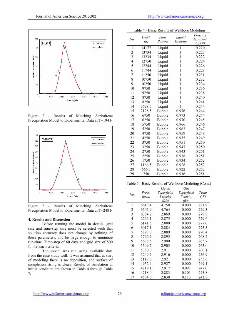
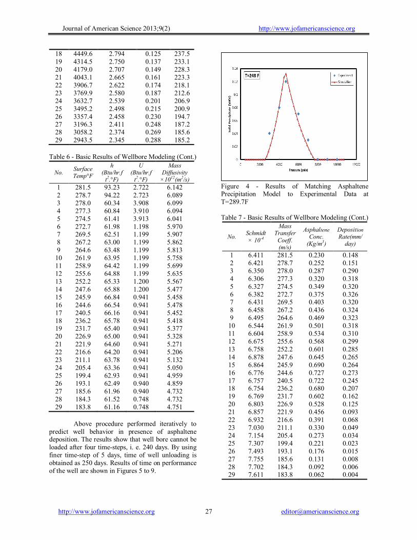
to experimental data, and plus fraction was split to C31+. For matching model to asphaltene precipitation data, new plus fraction split to non-precipitating fraction, C31A+, and precipitating fraction, C31B+. Crude oil composition after matching data is also shown in Table 3. Results of asphaltene precipitation matching are shown in Figures 2 to 4. This matched model was used for prediction of asphaltene precipitation from crude oil.
From Tables 4 to 7 it can be seen that surface temperature is not differing from fluid bulk temperature considerably. This is because of much larger amount of heat transfer coefficient, h, in comparison with overall heat transfer coefficient; U. Rate of deposition thickness is shown in Table 7 (Based on Eq. (8)). This data was used to estimate new wellbore diameter at the next time step, i. e. 60 days later, using Eq. (12).
Journal of American Science 2013;9(2) http://www.jofamericanscience.org
Figure 2 - Results of Matching Asphaltene Precipitation Model to Experimental Data at T=194 F Figure 3 - Results of Matching Asphaltene Precipitation Model to Experimental Data at T=248 F 4. Results and Discussion
Before running the model in details, grid size and time-step size must be selected such that solution accuracy does not change by refining of these parameters, and be large enough to minimize run-time. Time-step of 60 days and grid size of 500 ft. met such criteria.
The model was run using available data from the case study well. It was assumed that at start of modeling there is no deposition, and surface of completion string is clean. Results of simulation at initial condition are shown in Table 4 through Table 7.
predict well behavior in presence of asphaltene deposition. The results show that well bore cannot be loaded after four time-steps, i. e. 240 days. By using finer time-step of 5 days, time of well unloading is obtained as 250 days. Results of time on performance of the well are shown in Figures 5 to 9.
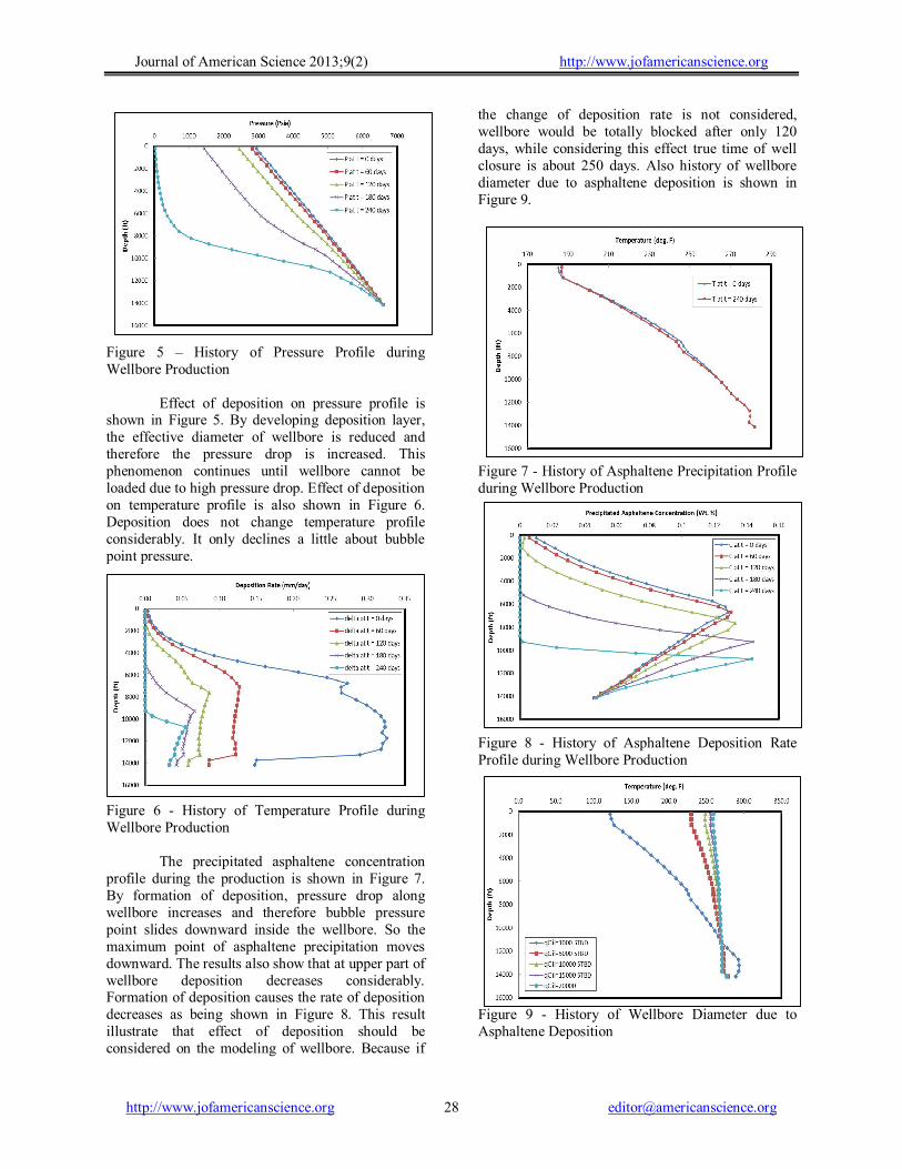
Figure 4 - Results of Matching Asphaltene Precipitation Model to Experimental Data at T=289.7F
Table 7 - Basic Results of Wellbore Modeling (Cont.)
Figure 5 – History of Pressure Profile during Wellbore Production
Effect of deposition on pressure profile is
shown in Figure 5. By developing deposition layer, the effective diameter of wellbore is reduced and therefore the pressure drop is increased. This phenomenon continues until wellbore cannot be loaded due to high pressure drop. Effect of deposition on temperature profile is also shown in Figure 6. Deposition does not change temperature profile considerably. It only declines a little about bubble point pressure.
Figure 6 - History of Temperature Profile during Wellbore Production
The precipitated asphaltene concentration profile during the production is shown in Figure 7. By formation of deposition, pressure drop along wellbore increases and therefore bubble pressure point slides downward inside the wellbore. So the maximum point of asphaltene precipitation moves downward. The results also show that at upper part of wellbore deposition decreases considerably. Formation of deposition causes the rate of deposition decreases as being shown in Figure 8. This result illustrate that effect of deposition should be considered on the modeling of wellbore. Because if
the change of deposition rate is not considered, wellbore would be totally blocked after only 120 days, while considering this effect true time of well closure is about 250 days. Also history of wellbore diameter due to asphaltene deposition is shown in Figure 9. Figure 7 - History of Asphaltene Precipitation Profile during Wellbore Production Figure 8 - History of Asphaltene Deposition Rate Profile during Wellbore Production Figure 9 - History of Wellbore Diameter due to Asphaltene Deposition
Journal of American Science 2013;9(2) http://www.jofamericanscience.org
Figure 10 - Effect of Fluid Velocity on Pressure Profile 5. Effect of Fluid Velocity
Jamialahmadi et al. (2009) investigate effect of single phase oil velocity on deposition of asphaltene and proposed an inverse proportionality. In one hand, increasing flow velocity simplifies the process of detachment of asphaltene particles from completion string and slows down deposition process. In the other hand, it changes pressure and temperature profile and asphaltene precipitation behavior. Thus an overall investigation of flow effect on pressure, temperature, asphaltene precipitation, and deposition rate has been investigated, and the results are shown in Figures 10 to 13.
Pressure profile declines due to increasing flow rate and bubble pressure point moves downward in wellbore (Figure 10). This phenomenon also slides maximum point of asphaltene precipitation downwardly (Figure 12). In Figure 13 asphaltene deposition profile can be divided into three regions. In 3 ½" tubing, fluid velocity is high, so deposition rate is low. In 4 ½" tubing, deposition can be divided into two regions. Before bubble point pressure, both of fluid velocity and asphaltene concentration increases, so their effects act opposing each other (based on Eq. (3)). In low flow rates, effect of increasing fluid velocity due to pressure drop is dominant and deposition rate decreases. At high flow rates, effect of asphaltene concentration is dominant and deposition rate increases gradually. After bubble point pressure fluid velocity increases and asphaltene concentration decreases. This means they act accordingly and, therefore, the rate of deposition decreases sharply.
Figure 11 - Effect of Fluid Velocity on Temperature Profile
Figure 12 - Effect of Fluid Velocity on Asphaltene Precipitation Profile Figure 13 - Effect of Fluid Velocity on Asphaltene Deposition Rate Profile
6. Conclusions
Developing a model for prediction of asphaltene deposition along the production well helps to understand the well behavior better. This can
Journal of American Science 2013;9(2) http://www.jofamericanscience.org
estimate the rate of deposition and time of well closure. In this work such model was used to simulate well behavior in details. It has been shown that surface temperature of well string does not differ considerably from fluid bulk temperature. Also effect of deposition on wellbore diameter was investigated, and it has been shown that wellbore diameter reduction must be considered to achieve exact time of well closure. The effect of fluid velocity on deposition rate has also been considered, and it is shown that how increasing fluid velocity can reduce rate of deposition.
Acknowledgements:
The authors would like to thank Dr. Rasoul Mokhtari for his help and support.
Corresponding Author: Saeid Dowlati Department of Petroleum Engineering Petroleum University of Technology Ahwaz, Iran E-mail: [email protected] Nomenclature A Area, ft2
B Formation Volume Factor D Pipe Diameter, in d Particle Diameter, µm
Logarithmic Mean of Two Areas, Perpendicular To Heat Transfer
C Concentration, Kg/m3
E Energy, J/mol f Friction Factor H Hold up h Heat Transfer Coefficient, Btu/hr.ft2.°F L Length, ft K Thermal Conductivity, Btu/hr.ft.°F
Boltzmann Constant = 1.38×10⁻²³
Coefficient in Eq. (3), m/s m Number of Time Steps
Mass Flux, Kg/m2.s Nu Nusselt Number n Number of Grids Pr Prandtl Number q Flow Rate, STBD R Universal Gas Constant = 8.314 J/mol.K Re Reynolds Number Sc Schmidt Number T Temperature, °F t Time, s U Overall Heat Transfer Coefficient,
Btu/hr.ft2.°F v Velocity, ft/s Wt% Composition in Weight Percent
Greek Letters β Mass Transfer Coefficient, m/s γ Specific Gravity Δx Layer Thickness, ft µ Viscosity, cp ρ Density, lb/ft3
Subscripts - Superscripts a activation o Oil g Gas l Liquid diff diffusion s Surface e Earth b Bulk d Deposition asph Asphaltene i Time Step Index j Grid Number Index k Iteration Number Index j±1/2 Inlet/Outlet of Grid p Particle References 1. Ansari, A. M., Sylvester, N.D., Sarica, C.,
Shoham, O., Brill, J. P. (1994). A Comprehensive Mechanistic Model for Upward Two-Phase Flow in Wellbores. SPE Production & Facilities Vol. 9. No. 2: 143-151.
2. Browarzik, D., Laux, H., Rahimian, I. (1999). Asphaltene flocculation in crude oil systems. Fluid Phase Equilibria 154: 285–300.
3. Bunger, J. W., Li, N.C. (1982). Chemistry of Asphaltene. Washington: Amer. Chemical Society.
4. Gomez, L. E., Shoham, O., Schmidt, Z., Chokshi, R. N., Brown, A., Northug, T. (1999). A Unified Mechanistic Model for Steady-State Two-Phase Flow in Wellbores and Pipelines. SPE 56520.
5. Hirschberg, A., deJong, L. N. J., Schipper, B. A., Meijer, J. G. (1984). Influence of Temperature and Pressure on Asphaltene Flocculation. SPE 11202: 283-293.
6. Jamialahmadi, M., Soltani Soulgani, B., Müller- Steinhagen, H., Rashtchian, D. (2009). Measurement and prediction of the rate of deposition of flocculated asphaltene particles from oil. International Journal of Heat and Mass Transfer 52: 4624–4634.
7. Katz, D. L., Saltman, W. (1939). Surface Tension of Hydrocarbons. Ind. Eng. Chem. 31: 91-94.
8. Kawanaka, S., Park, S.J., Mansoori, G.A. (1991). Organic deposition from reservoir fluids. SPE Reservoir Eng. J.: 185–192.
Journal of American Science 2013;9(2) http://www.jofamericanscience.org
9. Khalil, C. N., Rocha, N.O., Silva, E.B. (1997). Detection of Formation Damage Associated to Paraffin in Researvoir of the Reconcavo Baiano, SPE 37238.
10. Mansoori, G. A. (1999). Statistical Mechanical Models of Asphaltene Flocculation And Collapse From Petroleum Systems. Technical Meeting/Petroleum Conference of The South Saskatchewan Section, Regina.
11. Mullins, O. C., Sheu E. Y., Hammami, A., Marshall A. G. (2007). Asphaltenes, Heavy Oils and Petroleomics. New York: Springer.
12. Nghiem, L.X., Hassam, M.S., Nutakki, Ram. (1993). Efficient Modelling of Asphaltene Precipitation. SPE Annual Technical Conference and Exhibition.
13. Nghiem, L. X. (1999). Phase Behavior Modeling and Compositional Simulation of Asphaltene Precipitation in Reservoirs. PhD. Thesis. Alberta University.
14. Pan, H., Firoozabadi, A. (2001). Fast and Robust Algorithm for Compositional Modeling: Part II – Two-Phase Flash Computations. SPE 71603. SPE Annual Technical Conference and Exhibition.
15. Prandtl, L. (1944). Führer durch die Strömungslehre. Verlag Vieweg. Braunschweig.
16. Ramey, H. J. (1962). Wellbore Heat Transmission. SPE 96: 427–435.
17. Ramirez-Jaramillo, E., del Rio, J. M., Manero, O., Lira-Galeana, C. (2010). Effect of Deposition Geometry on Multiphase Flow of Wells Producing Asphaltenic and Waxy Oil Mixtures. Ind. Eng. Chem. Res. 49: 3391–3402.
18. Rassamdana, H., Dabir, B., Nematy, M., Farhami, M., Sahimi, M. (1996). Asphalt Flocculation and Deposition: I. The Onset of Precipitation. AIChE J42.
19. Soltani Soulgani, B., Rashtchian, D., Tohidi, B., Jamialahmadi, M. (2009). Integrated Modeling Methods for Asphaltene Deposition in Wellstring. Journal of the Japan Petroleum Institute 52: 322-331.
20. Speight, J. G. (1999). The Chemistry and Technology of Petroleum, Third Edition. New York: Marcel Dekker.
21. Vargas, F. M., Creek, J. L., Chapman, W. G. (2010). On the Development of an Asphaltene Deposition Simulator, Energy Fuels 24: 2294–2299.
22. Yen, T. F., Erdman, J. G., Pollack, S. S. (1961). Investigation of the structure of petroleum asphaltenes by X-ray diffraction. Anal. Chem. 33: 1587–1594.