TheGround Probing Radar (GPR) is a valuable tool for near surface geological, geotechnical, engineering, environ-mental, archaeological and other work. GPR images of the subsurface frequently contain geometric information(constant or variable-dip reflections) from various structures such as bedding, cracks, fractures etc. Such featuresare frequently the target of the survey; however, they are usually not good reflectors and they are highly localizedin time and in space. Their scale is therefore a factor significantly affecting their detectability. At the same time,the GPR method is very sensitive to broadband noise from buried small objects, electromagnetic anthropogenicactivity and systemic factors,which frequently blurs the reflections fromsuch targets. The purpose of this paper isto investigate the Curvelet Transform (CT) as a means of S/N enhancement and information retrieval from 2-DGPR sections, with particular emphasis on the recovery of features associated with specific temporal or spatialscales and geometry (orientation/dip).The CT is a multiscale and multidirectional expansion that formulates an optimally sparse representation of bi-variate functions with singularities on twice-differentiable (C2-continuous) curves (e.g. edges) and allows forthe optimal, whole or partial reconstruction of such objects. The CT can be viewed as a higher dimensional exten-sion of the wavelet transform: whereas discrete wavelets are isotropic and provide sparse representations offunctions with point singularities, curvelets are highly anisotropic and provide sparse representations of func-tions with singularities on curves. A GPR section essentially comprises a spatio-temporal sampling of the tran-sient wavefield which contains different arrivals that correspond to different interactions with wave scatterersin the subsurface (wavefronts). These are generally longitudinally piecewise smooth and transversely oscillatory,i.e. they comprise edges. Curvelets can detect wavefronts at different angles and scales because curvelets of agiven angle and scale locally correlate with aligned wavefronts of the same scale.The utility of the CT in processing noisy GPR data is investigatedwith software based on the Fast Discrete CT andadapted for use with a set of interactive driver functions that compute and display the curvelet decompositionand then allow the manipulation of data (wavefront) components at different scales and angles via the corre-sponding manipulation (cancellation or restoration) of their associated curvelets. The method is demonstratedwith data from archaeometric, geotechnical and hydrogeological surveys, contaminated by high levels of noise,or featuring straight and curved reflections in complex propagation media, or both. It is shown that the CT isvery effective in enhancing the S/N ratio by isolating and cancelling directional noise wavefronts of any scaleand angle of emergence, sometimes with surgical precision andwith particular reference to clutter. It can as suc-cessfully be used to retrievewaveforms of specific scale and geometry for further scrutiny, alsowith surgical pre-cision, as for instance distinguish signals from small and large aperture fractures and faults, different phases offracturing and faulting, bedding etc. Moreover, it can be useful in investigating the characteristics of signal prop-agation (hencematerial properties), albeit indirectly. This is possible because signal attenuation and temporal lo-calization are closely associated, so that scale and spatio-temporal localization are also closely related. Thus,interfaces embedded in low attenuation domains will tend to produce sharp reflections and fine-scale localiza-tion. Conversely, interfaces in high attenuation domains will tend to produce dull reflections with broadlocalization.
146 A. Tzanis / Journal of Applied Geophysics 115 (2015) 145–170
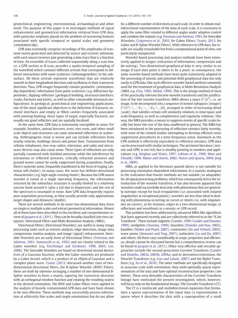
geotechnical, engineering, environmental, archaeological and otherwork. The purpose of this paper is to investigate methods of signalenhancement and geometrical information retrieval from GPR data,with particular emphasis placed on the problem of recovering featuresassociated with specific temporal or spatial scales and geometry(orientation/dip).
GPR data essentially comprise recordings of the amplitudes of tran-sient waves generated and detected by source and receiver antennae,with each source/receiver pair generating a data trace that is a functionof time. An ensemble of traces collected sequentially along a scan line,i.e. a GPR section or B-scan, provides a spatio-temporal sampling ofthe wavefield which contains different arrivals that correspond to dif-ferent interactions with wave scatterers (inhomogeneities) in the sub-surface. All these arrivals represent wavefronts that are relativelysmooth in their longitudinal direction and oscillatory in their transversedirection. Thus, GPR images frequently contain geometric (orientation/dip-dependent) information from point scatterers (e.g. diffraction hy-perbolae), dipping reflectors (geological bedding, structural interfaces,cracks, fractures and joints), aswell as other conceivable structural con-figurations. In geological, geotechnical and engineering applications,one of the most significant objectives is the detection of fractures, in-clined interfaces and empty or filled cavities frequently associatedwith jointing/faulting; these types of target, especially fractures, areusually not good reflectors and are spatially localized.
At the same time, GPR data is notoriously susceptible to noise. Forexample, boulders, animal burrows, trees, tree roots, and other smallscale objects and structures can cause unwanted reflections or scatter-ing. Anthropogenic noise is worse and can include reflections fromnearby vehicles, buildings, fences and power lines. Transmissions fromcellular telephones, two-way radios, television, and radio and micro-wave devices may also cause noise. These types of reflections are onlypartially countered with shielded antennae while the interference byextraneous or reflected airwaves, critically refracted airwaves andground waves cannot be easily suppressed during acquisition. Finally,there's systemic noise, frequentlymanifested in the form of ringing (an-tenna self-clutter). In many cases, the noise has definite directionalcharacteristics (e.g. high-angle crossing clutter). Because theGPR sourcewavelet is tuned at a single operating frequency, the informationreturned by the subsurface structure is usually limited to a relativelynarrow band around it (plus a tail due to dispersion) and the rest ofthe spectrum is swamped in noise. Raw GPR data frequently requirepost-acquisition processing, as they usually provide only approximatetarget shapes and distances (depths).
There are several methods to de-noise two dimensional data, focuson single ormultiple scales and extract geometrical information. Almostall of them have been described in the excellent and comprehensive re-viewof Jacques et al. (2011). They can be broadly classified into two cat-egories: Directional Filters and Multi-Resolution Analysis (MRA).
Directional Filters (Directional Wavelets) are useful in many imageprocessing tasks such as texture analysis, edge detection, image datacompression, motion analysis, and image (signal) enhancement. Steer-able Wavelets are an early form of Directional Filters (Freeman andAdelson, 1991; Simoncelli et al., 1992) and are closely related to theGabor wavelets (e.g. Feichtinger and Strohmer, 1998, 2003; Lee,2008). The Steerable Wavelets are based on directional second deriva-tives of a Gaussian function, while the Gabor wavelets are producedby a Gabor kernel, which is a product of an elliptical Gaussian and acomplex plane wave. Tzanis (2013) discussed another class of two-dimensional directional filters, the B-Spline Wavelet (BSW) Filters;these are built by sidewise arranging a number of one-dimensional B-Spline wavelets to form a matrix, tapering the transverse directionwith an orthogonal window function and rotating the resulting matrixto the desired orientation. The BSW and Gabor Filters were applied tothe analysis of heavily contaminated GPR data and have been shownto be very effective. These methods may successfully process informa-tion at arbitrarily fine scales and single orientations but do not allow
for a different number of directions at each scale. In order to obtainmul-tidirectional representation of the data at each scale, it is necessary toapply the same filter rotated to different angles under adaptive controland combine the outputs (e.g. Freeman and Adelson, 1991, for SteerableWavelets; Grigorescu et al., 2003, for Gabor Filters; Tzanis, 2013, forGabor and B-SplineWavelet Filters).With reference to GPR data, the re-sults are usually remarkable but froma computational point of view, notparticularly inexpensive.
Wavelet-based processing and analysis methods have been exten-sively applied to images (extraction of information, compression andde-noising). Two-dimensional geophysical data is very similar to animage if each data point is taken to be a pixel; in consequence, thesame wavelet-based methods have been quite extensively adapted tothe processing of seismic and potential-field geophysical data but onlyrarely to GPRdata. One such effectivewavelet-basedmethod commonlyused for the treatment of geophysical data, is Multi-Resolution Analysis(MRA, e.g. Chui, 1992; Mallat, 1999). This is the design method of mostof the practically relevant discrete wavelet transforms and the justifica-tion of the fast wavelet transform. MRA allows a space L2 ℝ2� �
, i.e. animage, to be decomposed into a sequence of nested subspaces (images)L2 ℝ2� �
⊃…⊃Vn⊃…⊃V0⊃… 0f g, arranged in order of increasing detail(scale), that satisfies certain self-similarity relations in time/space andscale/frequency, as well as completeness and regularity relations. Thisway, theMRA provides a means to suppress events of specific scales lo-cally but leave the rest of the data unaffected in general. The MRA hasbeen introduced to the processing of reflection seismics fairly recently,with most of the related studies attempting to develop efficient noisesuppression procedures in a time-frequency sense. Inasmuch as theGPR method is effectively equivalent to reflection seismics, GPR datacan be processedwith similar techniques. The pertinent literature (seis-mic and GPR) is not rich, but is steadily growing in numbers and appli-cations (e.g. Deighan and Watts, 1997; Leblanc et al., 1998; Miao andCheadle, 1998; Matos and Osorio, 2002; Nuzzo and Quarta, 2004; Jenget al., 2009).
MRA, as applied in the literature quoted above, is not suitable forprocessing orientation-dependent information. In a manner analogousto the realization that Fourier methods are not suitable (or adaptable)for all signal processing problems, which has consequently led to the in-troduction of the wavelet transform, it has also become apparent thatwavelets could successfully deal onlywith phenomena that are general-ly isotropic except for local irregularities (i.e. associated with isolatedsingularities at exceptional points); wavelets are less than ideal in deal-ing with phenomena occurring on curves or sheets (i.e. with singulari-ties on curves), as for instance, edges in a two-dimensional image, orreflections and wavefronts in a seismic or GPR record.
This problem has been addressed by advanced MRA-like algorithmsthat have appeared recently and are collectively referred to as the “X-letTransform”. These include ridgelets (Candès, 1999; Candès andDonoho,1999), wedgelets (Donoho, 1999), beamlets (Donoho and Huo, 2002),bandlets (Mallat and Peyré, 2007), contourlets (Do and Vetterli, 2005),wave atoms (Demanet and Ying, 2007), surfacelets (Lu and Do, 2007)and others. All these vary considerably in scope, properties and efficien-cy; details cannot be discussed herein but a comprehensive review canbe found in Jacques et al. (2011). Other very effective and versatile ap-proaches include the second generation Curvelet Transform (Candèsand Donoho, 2003a, 2003b, 2004a) and its derivatives/extensions, theShearlet Transform (e.g. Guo and Labate, 2007) and the Riplet Trans-form (e.g. Xu et al., 2010). The latter methods are specifically designedto associate scale with orientation; they yield optimally sparse repre-sentations of the data and have optimal reconstruction properties (seebelow). These very desirable characteristics of the Curvelet Transformlineage have motivated the present investigation, which, however,will focus only on the fundamental design: The Curvelet Transform(CT).
The CT is a multiscale and multidirectional expansion that formu-lates a sparse representation of the input data (a representation issparse when it describes the data with a superposition of a small
147A. Tzanis / Journal of Applied Geophysics 115 (2015) 145–170
number of components). The roots of the CT are traced to the field ofHarmonic Analysis, where curvelets were introduced as expansionsfor asymptotic solutions of wave equations (Smith, 1998; Candès,1999). In consequence, curvelets can be viewed as primitive and proto-type waveforms — they are local in both time/space and frequency/wavenumber and correspond to a partitioning of the 2D Fourier planeby highly anisotropic elements that obey the parabolic scaling principle,that is their width is proportional to the square of their length. Owing totheir anisotropic shape, curvelets are well adapted to detect wavefrontsat different angles and scales because curvelets at a given scale locallycorrelate with aligned wavefronts of the same scale (given thatwavefronts are actually edges in an otherwise smooth image).
Based on such properties of the curvelets, the CT provides anoptimally sparse representation of objects with edges — specifically ofobjects which are smooth except for discontinuities along generalcurves with bounded curvature (twice differentiable or C2-continuouscurve). If fm is the m-order curvelet approximation to an objectf(x1, x2)∈L2 ℝ2� �
, Candès and Donoho (2004a) show that if the objectis singular along a smooth C2 curve, the approximation error is ‖ f −fm‖2
2 = O(m−2[log m]3) and is optimal in the sense that there is noother representation of the same orderm, that can yield a smaller as-ymptotic error. This is far better than the O(m−1) error afforded bythe wavelet approximation. Optimal sparsity also implies that onecan recover curved objects from noisy data by curvelet shrinkage(analogous to wavelet shrinkage) and obtain a mean squared errorthat is far better than what was affordable with more traditionalmethods (Candès et al., 2006). In addition to the “static” view ofoptimal sparsity, curvelets may also formulate a “dynamic” optimal-ly sparse representation of wave propagators (e.g. Candès andDemanet, 2005; Sun et al., 2010): curvelets can model the geometryof wave propagation by translating the centre of the curvelet alongthe wave path. As Candès et al. (2006) point out, a physical interpre-tation of this result is that curvelets may be viewed as the represen-tation of local plane waves, with sufficient frequency localization tobehave like waves and sufficient spatial localization to simulta-neously behave like particles. The “dynamic” approach to curveletswill not be considered herein.
Another cardinal property of the CT is optimal image reconstructionin severely ill-posed problems; The CT possesses microlocal properties,(i.e. localization properties dependent on both position and orienta-tion), which render them particularly suitable for reconstructionproblems with missing data. In general terms, depending on the acqui-sition geometry and noise characteristics, the curvelet expansion can beseparated into a subset that can be recovered accurately, and one thatcannot. The microlocal properties of the curvelets allow the former (re-coverable) part to be reconstructedwith accuracy similar to the accura-cy thatwould be feasible if the datawas complete and noise-free. To thiseffect, Candès and Donoho (2004b) show that for some statisticalmodels which allow for C2 objects to be recovered, there are simple al-gorithms based on the shrinkage of curvelet biorthogonal decomposi-tions, which achieve optimal statistical rates of convergence, i.e. thereis no other estimating procedurewhich can return a fundamentally bet-ter mean square error.
The main body of this paper is organized as follows: The 2nd gener-ation CT will first be introduced in Section 2. Inasmuch as the applica-tion of the method is still uncommon in Exploration Geophysics atlarge and GPR practice in particular, the introduction will be relativelyrigorous; it will spare the reader from details and proofs but will elabo-rate on how curvelets are constructed and computed and how they op-erate on data with wavefronts. An introduction to the practicalimplementation of filtering via the CT will be given in Section 3. Thiswill be followed by a rigorous presentation of five applications(Section 4): the first three will concentrate on signal enhancementand information retrieval from data contaminated by high levels ofnoise; the last two will concentrate on information retrieval from datafeaturing straight and curved reflections in complex propagation
media. Finally, a discussion of the results and comparisons with othermethods developed with the same objective will conclude thepresentation.
2. The second generation Curvelet Transform
2.1. The continuous curvelet transform (CCT)
A curvelet frame is a wave packet frame on L2(ℝ2) based on a seconddyadic decomposition which, in effect, comprises an extension of theisotropic MRA concept to include anisotropic scaling and angular de-pendence (directionality) while maintaining rotational invariance. Inorder to construct the curvelet frame, a template (basic) curvelet is re-quired, which will generate it by translation, dilation and rotation. Theelements of the curvelet family will provide a partition (tiling) of thetwo-dimensional Fourier plane.
Consider a function f(x) ∈ L2(ℝ2) with x = [x1 x2]T and xj representspace or/and time. Next, consider the Fourier transformpair f(x)↔ F(ξ)where ξ= [ξ1 ξ2]T and ξj represent frequency or/and wavenumber. Letr= |ξ| be the radial coordinate and θ= arctan(ξ1, ξ2) be the azimuthalcoordinate in the ξ-plane. Finally, consider a partition of the polarcoordinate plane in concentric annuli (coronae) according to2j − 1 ≤ r ≤ 2j + 1, with each corona further partitioned into angularsectors according to ∠(θ,) ≤ 2− j/2, so as to generate polar wedges(Fig. 1a). The number of the wedges Nj increases like √(1/scale) anddoubles in every second ring so that the width of the wedges is propor-tional to the square of their length: this is the so called parabolic scaling(Fig. 1a).
Now consider a radial window W(r) and an angular window V(t),which must be smooth, nonnegative and real-valued. The support ofW is r ∈ (1/2, 2) and it must obey the admissibility condition∑j = −∞
∞ |W(2− jr)|2 = 1 for r N 0; the support of V is t ∈ (−2π, 2π]and the corresponding admissibility condition∑l = −∞
∞ V2(t − 2πl) = 1for t ∈ ℝ. There is no other theoretical limitation on the nature of thewindows, which means that they can be wavelets (e.g. as in Ma andPlonka, 2010).
The dilated basic curvelet in polar coordinates is
Φ j;l¼0;k¼0 r; θð Þ ¼ 2−3 j=4W 2− jr� �
V2 j=2θ2π
!;
r≥0; θ ∈ ½0;2πÞ; j ∈ ℕ0;
ð1Þ
with ⌊.⌋ denoting the floor operator (integer part). Evidently, W(2−jr)isolates ξ-values in the corona (2 j − 1, 2 j + 1). Likewise, V(2⌊j/2⌋θ)isolates ξ-values in the angular sector (−π2−⌊j/2⌋, π2−⌊j/2⌋). For increas-ing j and decreasing scale 2−j ∈ (0, 1], the breadth of W is growingand the width of V is shrinking, so that the wedges Φj,0,0(r,θ) becomelonger (see Fig. 1a and c): this is the effect of parabolic scaling.
The complete curvelet family in the ξ-domain is generated fromΦj,0,0 by dilation, rotation and translation according to:
Φ j;l;k r; θð Þ ¼ Φ j;0;0 Rθ j;lξ
� �� e−i x j;l
k ;ξh i; ð2aÞ
or, in terms of the radial and angular windows,
Φ j;l;k r; θð Þ ¼ 2−3 j=4W 2− jr� �
� V 2 j=2
2πθ−θlð Þ
!� e−i x j;l
k ;ξh i; ð2bÞ
where, θj,l=2πl ⋅ 2− ⌊j/2⌋, l=0,1,2,…, 0≤ θj,l b 2π, is a sequence of equi-spaced rotation angleswhose number varies proportionally to 1/√scale,
Rθ j;l¼ cos θ j;l sin θ j;l
− sin θ j;l cos θ j;l
� �; R−1
ϑ ¼ RTϑ ¼ R−θ;
Fig. 1. (a) Tiling of the ξ-plane in polar coordinateswith parabolic scaling. The shaded area represents awedge supporting a curvelet. (b) Schematic representation of a Cartesian grid in thex-domain, associated with a ξ-domain wedge like the shaded one shown in Fig. 1a. Due to the duality between the two domains, the spacing and scaling of the x-domain curvelet(represented by the ellipse) is also parabolic. (c) Some ξ-domain curvelets in perspective view: from left to right they are { j = 1, l = 0}, { j = 2, l = 2}, { j = 3, l = 0} and { j = 4, l =22}. (d) The x-domain curvelets {j = 2, l = 2} (left) and an arbitrarily translated version of {j = 4, l = 22} (right).
148 A. Tzanis / Journal of Applied Geophysics 115 (2015) 145–170
is the rotation by θj,l radians and
x j;lk ¼ R−1
θl2− j 00 2− j=2
� �k1k2
� �
are scaled positions with k1; k2 ∈ℤ2 representing the translation param-eters. As evident in Eqs. (2a) and (2b), the angularwindowVnow isolatesξ-values in the angular sector−π2−⌊j/2⌋≤ θ− θj,l≤ π2−⌊j/2⌋. Moreover, thesupport ofΦj,l,k does not depend on the translation parameters at all.
In the x-domain, the curvelet comprises a waveform defined by theFourier Transform of Φ:
φ j;l;k xð Þ ¼ φ j;0;0 Rθl x−x j;lk
� �� �: ð3Þ
Inasmuch as the support of Φj,l,k is independent of k, the frequencylocalization of Φj,l,0 is such that φj,l,0(x) will decay rapidly outside arectangle of size 2− j × 2− j/2 with its major axis perpendicular to thepolar angle θj,l (e.g. Fig. 1b and d). Thus, the effective size of φj,l,k(x)will also obey the parabolic scaling relationships: length ≈ 2− j/2,width ≈ 2− j ⇒ width ≈ length2. Moreover, Φj,0,0 is by constructionsupported away from the ξ2 axis (where ξ1 = 0) but near the ξ1axis (where ξ2 = 0). Therefore, φj,0,0 (x) will oscillate in the x2-direction and will be low-pass in the x1-direction. As evident fromEqs. (2a) and (2b), these oscillation properties are preserved during
rotation and translation (e.g. Fig. 1d). Then, at any scale 2−j, a curveletwillbe enveloped by a ridgewith effective length 2−j/2 andwidth 2−j andwilloscillate in a direction perpendicular to that ridge (see Fig. 1d).
A last matter to be considered is the “hole” arising in the ξ-planearound zero, since the rotations of the basic curvelets are defined onlyfor the scales 2−j. For a complete covering of the ξ-plane onemust definea low-pass elementWj0 which is supported on the unit circle and is non-directional (isotropic). This (coarsest scale) element obeys
W j0rð Þ
��� ���2 þXjN j0
W 2− jr� ���� ���2 ¼ 1; ð4Þ
so that coarsest scale curvelet will be
Φ j0ξð Þ ¼ 2− j0W j
02− j0 ξj j� �
;
and will admit a x-domain representation of the form
φ j0 ;kxð Þ ¼ φ j0
x−2− j0k� �
:
Based on the above construction principles, a curvelet coefficient com-prises the inner product between f(x1, x2) and a curvelet φj,l,k, j N j0:
c j; l; kð Þ ¼ f ;φ j;l;k
D E¼Zℝ2
f xð Þφ j;l;k xð Þdx: ð5Þ
149A. Tzanis / Journal of Applied Geophysics 115 (2015) 145–170
The inverse continuous curvelet transform will then be defined bythe reconstruction rule
f xð Þ ¼X
j≥ j0 ;l;k
c j; l; kð Þφ j;l;k xð Þ; ð6Þ
while the Parseval condition ∑j;l;k
c j; l; kð Þj j2 ¼ fk k2L2 ℝ2ð Þ will hold for all
f ∈ L2(ℝ2) ensuring a tight frame property. As a result of the parabolicscaling, the curvelet frame is an optimally sparse representation forfunctions with singularities along curves but otherwise smooth(Candès and Demanet, 2005).
2.2. The discrete curvelet transform (DCT)
The formulation of the CCT is not particularly suitable for measured2-D data which is usually obtained in the form of rectangular (Carte-sian) arrays, because circular coronae and rotation are not easily adapt-able to Cartesian geometries. In response, the inventors of the curvelettransform also developed discrete formulations which are suitable forCartesian data arrays while being faithful to the mathematical formal-ism of the CCT.
In these formulations, the circular coronae are replaced by rectangu-lar “coronae” (concentric rectangular annuli) and the rotations are re-placed by shearing, so as to generate a pseudo-polar grid like the oneshown in Fig. 2a. Thus, the Cartesian equivalent of the radial windowW is
where U(ξ) = u(2−jξ1) ⋅ u(2−jξ2) and u is a low-pass one-dimensionalwindow that obeys 0≤ u≤ 1 and vanishes for all ξ∉ [−2, 2]. Under this
definition and on including the isotropic windowfW j0ξð Þ, of the coarsest
scale, the Cartesian analogue of the admissibility condition (4) reads
fW2j0ξð Þ þ
XjN j0fW2
j ξð Þ ¼ 1 ð7Þ
Fig. 2. (a) Pseudo-polar partitioning (tiling) of the ξ-plane in Cartesian coordinates with trapindexing of thewedges (l) counts clockwise from the top-left corner of each scale. The solid blacthat support the curvelets shown in (b). The grey partitions indicate the wedges supporting th
and can be shown to hold for all ξ. The angular window V is now takento be
V j ξð Þ ¼ V 2⌊ j=2⌋ ξ2ξ1
�:
Following the above definitions, the basic curvelet in Cartesian coor-dinates is
eΦ j;l¼0;k¼0 ξð Þ ¼ 2−3 j=4 �fW j ξð Þ � V j ξð Þ
and is supported on a trapezoidal wedges bounded as ξ1; ξ2ð Þ : 2 j≤ξ1≤n
2 jþ1; −2− j=2≤ ξ2
ξ1≤2− j=2g, isolating the ξ-values included therein.
In order to map the basic Cartesian curvelet onto different orienta-tions, instead of equispaced angles define a set of equi-spaced slopestan θl = l ⋅ 2⌊ − j/2⌋,l = −2⌊j/2⌋,…,2⌊j/2⌋ − 1 and define
eΦ j;l;k¼0 ξð Þ ¼ eΦ j;0;0 Sθlξ� �
ð8aÞ
where
Sθl ¼1 0
− tanθl 1
� �is the shear matrix and where the admissibility condition is upheld.
Eq. (8a) can be written in terms of the windowsfW and V as
and clearly isolates ξ-values in the wedge ξ1; ξ2ð Þ : 2 j≤ξ1≤2 jþ1;
n−2− j=2≤ ξ2
ξ1− tan θl≤2− j=2g:
Constructions such as those implied by Eqs. (8a) and (8b) are il-lustrated in Fig. 2b. In order to define the Cartesian analogues of
the familyΦ j;l;0 ¼ Φ j;0;0 Rθ j;lξ
� �described in Section 2.1, it is sufficient
ezoidal wedges. The inner (coarsest-scale) isotropic partition corresponds to j = 1. Thek partitions at j=3, l=5and j=3, l=15 indicate the right-hand side trapezoidal wedgese curvelets shown in Fig. 3.
150 A. Tzanis / Journal of Applied Geophysics 115 (2015) 145–170
to complete the curvelets eΦ j;l;k¼0 ξð Þ by symmetry with respect to the
origin and rotation by ±π/2 radians. The complete family eΦ j;l;k¼0 ξð Þgenerates the concentric partitioning whose geometry is shown inFig. 2a.
In a final step, on introducing the translation parameters
ex j;lk ¼ S−T
θl2− j 00 2− j=2
� �k1k2
� �¼ S−T
θl b jk;
and using Eq. (8b), the Cartesian equivalent of Eqs. (2a) and (2b) can bewritten thus:
eΦ j;l;k ξð Þ ¼ eΦ j;0;0 Sθlξ� �
� e−i ex j;lk ;ξ
� :
Aswith its CCT counterpart, the x-domain representation of the Car-tesian curvelet comprises a waveform defined by the Fourier Transform
of eΦ and is:
eφ j;l;k xð Þ ¼ eφ j;0;0 STθl x−ex j;lk
� �� �:
It follows that the discrete Cartesian counterpart of the curvelet co-efficients is:
ec j; l; kð Þ ¼ f ; eφ j;l;k
D E¼Xx1 ;x2
f xð Þeφ j;l;k xð Þ: ð9Þ
Finally, the inverse discrete curvelet transform is defined by a recon-struction formula analogous to Eq. (6):
f xð Þ ¼X
j≥ j0 ;l;k
ec j; l; kð Þeφ j;l;k xð Þ: ð10Þ
The implementation of Eq. (9) is not straightforward; the difficulty isthat on using the two-dimensional Fourier Transform to obtain eφ j;l;k xð Þfrom eΦ j;l;k ξð Þ, one would need to evaluate the FFT on the sheared gridex j;lk , where it cannot be applied. In response, two indirect solutions
have been developed by Candès et al. (2006): the unequi-spaced FFTmethod and the wrapping method.
In the USFFT method, the translation grid is rotated so as to alignwith the orientation of the curvelet. To do this, at each scale/angle pair(j, l) the implementation uses a non-standard interpolation scheme to
obtain sampled values of F(ξ) over the support of eΦ j;l;k ξð Þ. The inversetransform also uses conjugate gradients iteration to invert the interpo-lation step. In consequence, the USFFTmethod has a rather higher com-putational cost than the wrapping algorithm.
In the wrapping method the translation grid remains untilted andthe same for every orientation albeit each curvelet is assigned with itsproper angle. The curvelet coefficients are taken as per Eq. (9), except
that ex j;lk is replaced by bk
j = (k12−j, k22−j/2) with b taking values on arectangular grid. In this case, however, it is apparent that the windoweΦ j;l;k ξð Þ cannot fit into a rectangle of size 2j × 2j/2 to which an inverseFFT could be applied. The wrapping algorithm addresses this problem
by periodizing the windowed ξ-domain coefficients eC j;l ξð Þ ¼ F ξð ÞeΦ j;l;k
ξð Þ and re-indexing eC j;l bywrapping it around a rectangle centred at the
origin and approximately equal to 2j× 2j/2. If F(ξ) is unity, then eC j;l ξð Þ ¼eΦ j;l;k ξð Þ and a x-domain representation of the curvelet can be obtainedby inverse FFT, otherwise the curvelet coefficients are obtained by in-
verse FFT of eC j;l ξð Þ. Fig. 3a presents examples of curvelets computedwith the wrapping method at different scales, orientations and (arbi-trary) translations.
Fig. 3b shows how curvelets interact with data and elongate curvedobjects in particular. Specifically, panel (i) illustrates a contrived
512 × 512 data set featuring awavy up-dipping set of intermittent reflec-tions. The data was decomposed into six scales with the second coarsestscale ( j = 2) comprising 24 angles (six per quadrant) and the numberof angles doubling in every second scale. As evident from theprevious dis-cussion, curvelets are elongate and slender waveforms with length pro-portional to 2-−j/2 and width proportional to 2−j; they oscillate in theirtransverse direction and are low-pass in their longitudinal direction.Curvelets can interact with curved objects in three ways:
1. When the curvelet and the object intersect while aligned parallel totheir longitudinal directions, the transverse oscillatory part of thecurvelet will locally match the same-scale component of the objectand will encode the information in the corresponding set of curveletcoefficients which will have significant amplitudes.
2. When the curvelet and the object intersect at an arbitrary angle, thematching of the same-scale content will be imperfect and informa-tion will be lost to the curvelet's low-pass longitudinal action: thecurvelet coefficients will have small amplitudes.
3. When the curvelet and the object do not intersect, the coefficientswill be near zero.
Due to the unique orientational characteristics of this data set, only ahandful of coefficients have noteworthy amplitudes. As an example, inFig. 3b-ii the left panel illustrates the coefficients { j = 4, l = 5} andthe right panel a partial reconstruction based on these coefficientsonly. The associated curvelet has a slope of−110° and is almost perfect-ly aligned with the main trend of the “reflections” shown in Fig. 3b-i. Inconsequence, it extracts a clear and strong component of the signal.Conversely, the left panel of Fig. 3b-iii illustrates the coefficients {j =4, l = 7} and the right panel the corresponding partial reconstructionof the data. The associated curvelet has a slope of −94° and isintercepting the reflections at an angle of 14°; evidently, it cannotmatch a signal component of any significant amplitude and the coeffi-cients and reconstruction have very low amplitudes. Finally, the leftpanel of Fig. 3b-iv illustrates the coefficients { j = 3, l = 5} and theright panel the corresponding partial reconstruction. The associatedcurvelet is perfectly aligned with the main reflections but has thewrong scale: it extracts only a very weak background component asso-ciated with the longer ξ-components of the data. It turns out that thedata can be reconstructed to within 96% from the coefficients { j = 3,l = 4–6}. This demonstrates how curvelets may assist in the retrievalof scale-and-orientation dependent information from GPR data.
An additional significant observation to be made in Fig. 3b is the fol-lowing: The images of the curvelet coefficients and reconstructions, allcontain a “side lobe” structure above the left and below the right endof the reconstructed up-dipping synthetic waveform. Itmust be empha-sized that these are not artefacts but proper features of the reconstruc-tion. Note that the synthetic waveform shown in Fig. 3b-i is actuallytruncated at the left and right ends of the image, i.e. it is incomplete.However, because themain part of thewaveform contains sufficient in-formation, the reconstruction rebuilds the missing ends and becausethere is no room to fit them in the 512 × 512 data matrix, it foldsthem around the edges. This is a powerful demonstration of the optimalreconstruction afforded by the Curvelet Transform and empirical justifi-cation of the statementmade in the Introduction, that “… the microlocalproperties of the curvelets allow the recoverable part [of the data] to be re-constructed with accuracy similar to the accuracy that would be feasible ifthe data was complete and noise-free”.
3. GPR data analysis with the Curvelet Transform
The DCT has been implemented in the software packageCurveLab, written by E. Candés, L. Demanet and L. Ying and availableat http://www.curvelet.org. The package contains Matlab and C++implementations of both the USFFT and Wrapping methods. In thework presented herein, only the wrapping method has been imple-mented for being computationally more efficient. The utility of the CT
Fig. 3. a. (i) Amplitudes of complex ξ-domain curvelets at different scales and orientations. The trapezoidal wedges supporting these curvelets are shown in Fig. 2a. The indexing (l) in-creases clockwise from the top-left corner of each scale. (ii) Arbitrarily translated x-domain curvelets, corresponding to the ξ-domain curvelets of the left panel (i). b. A demonstrationof data and curvelet interactions. (i) The data comprise a 512 × 512matrix featuring only a set of wavy intermittent up-dipping reflections. (ii) The coefficients, (left) and a partial recon-struction of the data (right) generated by the curvelet { j = 4, l = 5}. (iii) As in (ii) but for { j = 4, l = 7}. (iv) As in (ii) and (iii) but for { j = 3, l = 5}.
151A. Tzanis / Journal of Applied Geophysics 115 (2015) 145–170
will be demonstrated via a piece of software specifically developed tofacilitate the interactive application of the DCT and to visualize and con-trol the process; a fully functional version of this application is alreadyavailable in the matGPR software (e.g. Tzanis, 2010), currently locatedat http://users.uoa.gr/~atzanis/matgpr/matgpr.html.
For a given dataset, the software prompts for the number of scales,with j = 1 corresponding to the (coarsest-scale) inner isotropic parti-tion. It also inquires for the number of angles at the second coarserscale (j = 2), i.e. the first scale at which an angular decomposition iscomputed (the number of angles doubles in every second scale). TheDCT is then computed with the option that yields real-valued curveletcoefficients: at any given scale, if L is the number of angles, thenthere will be L/2 ‘cosine’ coefficients stored with indices 1 … L/2, as
well as L/2 ‘sine’ coefficients stored by symmetry of L/2 with indicesL/2 + 1 … L. The coefficients are indexed in a clockwise sensestarting at the top-left corner of the north quadrant and are arrangedso that the indices l = 1 … L/2 of the cosine coefficients span thenorth and east quadrants and the indices l= L/2+ 1… L of the sine co-efficients span the south and west quadrants. Thus, each element of thedata reconstruction rule specified by Eq. (10) can be completely speci-fied by the pair (l, L/2 + 1) of sine and cosine coefficients.
The finest level scale extracts the highest frequency/longest wave-number content. The design of appropriate basis functions at the outer-most dyadic corona is not straightforward due to difficulties relating toissues of over- or under-sampling at the high-ξ end of the spectrum(Candès et al., 2006). One apparent solution is to assign wavelets
Fig. 4. The upper-right diagonal (north and east quadrants) of the pseudo-polar tiling ofthe ξ-plane for a 512-by-512 data matrix decomposed into six scales and 24 angles atthe second coarser scale (j=2). The tiling is drawn in data matrix coordinates and all an-gles and slopes refer to matrix coordinates (see text for details). Each trapezoidal wedge,as well as the rectangles corresponding to j=1 (central) and j=6 (lower left), is associ-ated with a corresponding set of sine and cosine coefficients and functions as a “graphicalswitch” whose state can be toggled by pointing and clicking. The “On” state is indicatedwith shading and the corresponding coefficients are included in a reconstruction of theinput data. The “Off” state is blank and the corresponding coefficients are excluded froma reconstruction.
152 A. Tzanis / Journal of Applied Geophysics 115 (2015) 145–170
instead of curvelets to the finest scale and treat it with isotropic
Cartesian windows fW Je ξð Þ constructed so that fW2Jeξð Þ, together with
the curveletwindows, form a partition of unity as in Eq. (7). Thewaveletcoefficients can, then, be obtained by inverse FFT. This approach is sim-ple but not consistent with the idea of directional basis elements at thefinest scale. Proper curvelet-based remedies for tiling the finest scalehave been proposed by Candès et al. (2006). Note, however, that GPRdata is usually oversampled, at leastwith respect to the central frequen-cy of the Tx antenna. In consequence, there is little (if any) useful infor-mation at the high frequency/long wavenumber scales which usuallycomprise random noise. In response, the wavelet-based remedy forthe finest level scale was also adopted in this implementation of theDCT.
After the DCT is computed, the upper-right diagonal of the (pseudo-polar) tiling of the ξ-plane is displayed as shown in Fig. 4 for a hypothet-ical 512-by-512 datamatrix decomposed into six scales and 24 angles atthe second coarser scale. The lower-left diagonal does not contain inde-pendent information and is redundant (see above). It is very importantto clarify that the tiling is drawn in data matrix coordinates and not in
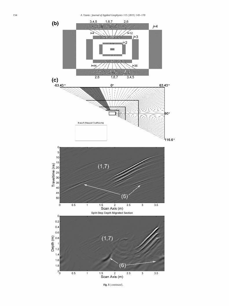
Fig. 5. a. Top: Synthetic structural model used for demonstrating the application of the Curveletterm of the phase velocity and are described in Table 1. Middle: Synthetic zero-offset radargrKnight (2006); the central frequency is 400MHz. Bottom: The synthetic radargram after 2-D degenerated by the DCT of the synthetic radargram of Fig. 5a; only the scales j= 1 to j= 4 are shquadrants (upper-right diagonal). The sine coefficients are arranged in the south and west quasynthetic radargram for scales j=3and j=4are also indicated. c. Top: The selection of coefficieare represented by the subset of trapezoidal wedges {j = 3, l ∈ [4, 6]} ∪ {j = 4, l ∈ [4, 6]} ∪ {jselection of curvelet coefficients shown at the top; the reconstruction includes complete infor2-D split-step depth migration. d. Top: The coefficients used for isolating information about crazoidalwedges {j=3, l∈ [10, 12]}∪ {j=4, l∈ [10, 12]}∪ {j=5, l∈ [19, 24]}.Middle: Partial recoat the top; the reconstruction includes complete information about crack 2, partial informationgration of the reconstructed synthetic radargram. e. Spurious oscillation due to narrow-bandfiltsynthetic radargram of Fig. 5a. The subset {j=1} ∪ {j=2, l∈ [1, 16]}∪ {j=5, l∈ [7, 12]} is excthe back arrow points to the low amplitude spurious oscillation generated by the narrow band
physical coordinates of wavenumber and frequency. Likewise, all theangles (slopes) indicated in the drawing refer to data matrix coordi-nates. To seewhy, consider that in the discrete (digital) implementationof the CT, the curvelet decomposition can only be configured in matrixcoordinates (just like in any other digital operation). Accordingly, inthe ξ2-axis representing frequency, the Nyquist is n2/2, n2 ∈ ℕ, andthe frequency range varies with integer steps in the interval [−n2/2,n2/2]. Likewise, in the ξ1-axis representing wavenumber, the Nyquistis n1/2, n1 ∈ ℕ , and the wavenumber varies with integer steps in[−n1/2, n1/2]. It follows that the dimensions of the data matrix arevery important in determining the angular partitioning of each scale.With n2 × n1 denoting the order of rows and columns, a 512 × 512 ma-trix has different angular partitioning than a 512× 1024 or a 1024× 512matrix. In the first case the partitioning along the frequency and wave-number axes is identical. In the second case the partitioning is more de-tailed along the wavenumber axis and in the third case it is moredetailed along the frequency axis. A corollary of this point is that insome cases it may be advisable to appropriately resample the data soas to better focus on its temporal or spatial details.
Each trapezoidalwedge shown in Fig. 4 is a graphical object that rep-resents the support of the curvelet used to generate its associated set ofcoefficients: at each scale the lth graphical object (wedge) is assignedwith the indices of the corresponding cosine (l) and sine (L/2 + l) coef-ficients, while it is also set up to function as a virtual switch whose On/Off state is controlled by the screen pointing device (e.g. themouse). Allthe wedges are initially displayed in their ‘On’ state, which is indicatedby shading. The ‘Off’ state is indicated by a blank wedge. The coarsestlevel isotropic partition is displayed as a rectangle at the centre of thetile. The finest level scale is displayed separately at the space thatwould have been occupied by the redundant lower-left diagonal and il-lustrates the associated set of wavelet coefficients. Both the coarsest andfinest scale objects function as virtual switches just like the trapezoidalwedges.
It is possible to decidewhich coefficients to include (exclude) from aprocessed (reconstructed) version of the input data by pointing andclicking inside a trapezoidal wedge or rectangle. If the switch is ‘On’,this will shrink the associated sets of cosine and sine coefficients by afactor ∈ [0, 1] and will toggle its state to ‘Off’, blanking it out as shownin Fig. 4. This is amanual curvelet shrinkage approach. The shrinking fac-tor is specified by the analyst and can be changed during runtime. Thedefault value is zero (complete negation of the selected coefficients)and all applications to be shown herein use the default value. Theshrunk (or negated) coefficients may be restored by clicking inside ablank switch, in which case its state is reset to ‘On’ (shaded). It is alsopossible to toggle entire scales or angular subsets of a scale, by using ap-propriate GUI controls (not shown in Fig. 4). A partial or whole recon-struction of the data can be computed at any time, with GUI controlsalso not shown.
The application of the DCT to the analysis of GPR data will now bedemonstrated with a complex synthetic radargram. Non-randomnoise is very difficult to simulate realistically and will not concern thisexample; the problem will be addressed in Section 4, in associationwith the treatment of real (observed) radargrams. Moreover, because
Transform. The objects comprising themodel are shaded according to the non-dispersiveam generated from the model shown at the top panel with the FDTD solver of Irving andpthmigration with the split-stepmethod (see text for details). b. The curvelet coefficientsown for the sake of readability. The cosine coefficients are arranged in the north and eastdrants (lower-left diagonal). The coefficients encoding the structural elements 1–7 of thents used for the extraction of cracks 3, 4 and 5 from the synthetic radargramof Fig. 5a; they= 5, l ∈ [7, 12]}. Middle: Partial reconstruction of the synthetic radargram based on themation about cracks 3, 4 and 5 only. Bottom: The partially reconstructed radargram afterck 2 from the synthetic radargram of Fig. 5a; they are represented by the subset of trape-nstruction of the synthetic radargrambased on the selection of curvelet coefficients shownabout the bedrock (object 6) and a ghost of object 7 (cavity). Bottom: Split-step depth mi-ering of a transientwavefield. Top: The coefficients used in the partial reconstruction of theluded from the reconstruction. Bottom: Partial reconstruction of the synthetic radargram;-stopping operation.
153A. Tzanis / Journal of Applied Geophysics 115 (2015) 145–170
a basic idea (andmotivation) for implementing the CT is the manipula-tion and extraction of geometrical information, the analysis will bemainly focused on its angular resolution capability. The model usedfor generating the synthetic example is illustrated at the top of Fig. 5aand is summarized in Table 1. It consists of seven closely spaced geo-metrical objects with diverse material properties and orientations, em-bedded in a backgroundwith “average”material properties. The objectsare so arranged, as to generate overlapping of wavefronts and clutter.This is useful in clarifying the reconstructive capacity, as well as the ex-tent and limitations of the angular discriminative capacity affordable by
the CT. It is will also be useful in pointing out and discussing the outputof the analysis with particular attention to the case of highly anisotropicfiltering.
The zero-offset synthetic radargram was computed for a nominalcentral frequency of 400MHzwith the time domain Finite Difference al-gorithm of Irving and Knight (2006) as implemented in the matGPRsoftware (Tzanis, 2010). The synthetic section is shown in the middlepanel of Fig. 5a after deconvolving the surface reflection; it comprisesa 256 sample × 512 trace matrix with a sampling rate of 0.2149 nsand a trace spacing of 0.007436 m. The principal wavefronts
Fig. 5 (continued).
154 A. Tzanis / Journal of Applied Geophysics 115 (2015) 145–170
155A. Tzanis / Journal of Applied Geophysics 115 (2015) 145–170
Fig. 5 (continued).
156 A. Tzanis / Journal of Applied Geophysics 115 (2015) 145–170
(reflections) corresponding to the objects of Fig. 5a are clearly discern-ible and pointed to. In addition, minor irregularities in the shape of ob-jects 6 and 7, reverberation between cracks and scattering at the tipsand intersections of the cracks also generates a significant amount oflower amplitude secondary wavefronts that take the form of crossingclutter.
The velocity structure is exactly known, therefore, it is possible todetermine the amount of structural information recoverable from theradargram. Depth migration is a suitable approach and the matGPR im-plementation of the Split-Step method of Stoffa et al. (1990) was used,which is augmented to account for the frequency dependence of thephase velocity based on the formulation of Bano (1996). The depth-migrated radargram is shown at the bottom of Fig. 5a. The locationand geometry of all objects is generally recovered with success but notwith equal accuracy. Specifically, the lower tips of cracks 2, 3, 4 and 5are disturbed by artefacts which are, at least partially produced by the
Table 1Description and properties of the objects comprising the synthetic model of Fig. 5a. The velocit
Object Description Dip (°)
0 Background −1 Short, thin dielectric crack. −17°2 Dielectric crack. 21°3 Thin crack with moist argillaceous material −45°4 Crack with moist argillaceous material −45°5 Thick crack with moist argillaceous material −45°6 Dielectric bedrock Variable (undula7 Elongate cavity with moist ferriferous material (laterite) Quasi-horizontal
interaction of their respective wavefronts with the wavefront of object6 (bedrock) andwith the clutter. Moreover, the interference of the clut-ter can clearly be seen in the images of cracks 3, 4 and 5, although it doesnot obscure them. Analogous but smaller scale effects can be observedaround the centralmound of the bedrock and at the lower surface of ob-ject 7 (cavity). The sub-vertical left and right interfaces of object 7 donot reflect signals from overhead sources and cannot be imaged.
The synthetic radargram was decomposed into six scales with thesecond coarser (j = 2) scale comprising 32 angular wedges; the rela-tively fine angular decomposition is necessary because the scatterers(objects) are tightly spaced. In order to visualize how curvelet coeffi-cients are stored and how they encode information, Fig. 5b shows thecomplete set for scales j=1 to j=4. It is apparent that significant infor-mation about the amplitude and geometry of the wavefronts compris-ing the radargram exists only in the north and south quadrants ofscales j=3 and j=4. It must be emphasized that analogous significant
y and quality factors are calculated after Bano (1996).
157A. Tzanis / Journal of Applied Geophysics 115 (2015) 145–170
information exists in the same quadrants of the finer fifth scale (j = 5)which is not shown because the figure would then be rather difficult toread. The coefficients of the sixth scale are not curvelets; they are wave-lets (isotropic) and at the relevant frequencies/wavenumbers representlow-amplitude random noise. The cosine coefficients are arranged inthe north and east quadrants (upper-right diagonal) and for j = 3 andj = 4 are indexed from l = 1 to l = 32 with respect to the NW corner.The sine coefficients are arranged in the south and west quadrantsand for j = 3 and j = 4 are indexed from l = 33 to l = 64. The coeffi-cients representing the structural elements 1–7 of the radargram atthese scales are also indicated in the figure.
Cracks 3, 4 and 5 have distinct orientational characteristics and theycan be effectively isolated from the other structural elements of theradargram, as demonstrated in Fig. 5b and c. The top panel of Fig. 5cshows the selection of coefficients used for the partial reconstructiondisplayed in themiddle: this is represented by the subset of trapezoidalwedges {j=3, l∈ [4, 6]}∪ {j=4, l∈ [4, 6]}∪ {j=5, l∈ [7, 12]}, with allthe rest having been shrunk to zero. Although for the sake of simplicitythewedges are indexed only in the north and east quadrants, from l=1to l= L2, it is always important to bear in mind that each wedge repre-sents the pair (l, L/2 + l) of cosine and sine coefficients that is actuallyused in the reconstruction. It is immediately apparent that the mainpart of the wavefronts generated by cracks 3, 4 and 5 is very efficientlyreproduced and that the optimal reconstruction property of the CT haseffectively eliminated interference by wavefronts from the other struc-tural elements of themodel. This is also clearly observed in themigratedradargram shown at the bottom, in which the images of the cracks aresharper and better focused and the artefacts associated with theirlower tips are significantly reduced. However, they are not eliminatedbecause the curvelets used in the analysis did not (and could not) elim-inate the matching orientational attributes of the interference. Diffrac-tions from the upper tips of the cracks have not been included in thereconstruction; evidently, this does not (and could not) affect the qual-ity of the result. In addition, there are very few matching orientationalcharacteristics between cracks 3, 4 and 5 and the other structural ele-ments, which could be encoded in the coefficients and appear in the re-constructed image: these are clearly marked and include shortsegments of object 6 and ghosts of objects 1 and 7.
In the next example, the target of the analysis is crack 2, whichshares some orientational attributes with the bedrock (object 6). Themiddle panel of Fig. 5d shows a partial reconstruction based on the co-efficients represented by thewedges shown at the top; these are { j=3,l∈ [10, 12]} ∪ {j=4, l∈ [10, 12]} ∪ {j=5, l∈ [19, 24]} with all the resthaving been shrunk to zero. The wavefront generated by crack 2 is effi-ciently reproduced and is free of any interference caused by the otherstructural elements and the clutter; the artefact associated with itslower tip is also significantly suppressed (bottom). The matchingdown-dipping orientational attributes of the bedrock are also encodedin the coefficients and included in the reconstruction, as indicated inthe middle and bottom panels respectively. For the same reason, onecan also observe a ghost of object 7 and, at the top right of the recon-structed and depth migrated radargrams, ghosts of the upper tips ofcracks 3 and 4; the latter are due to the down-dipping parts of the dif-fraction fronts associated with the tips of these cracks and are clearlyvisible at the extreme right of the reconstructed radargram (middle).
It is significant to point out that the forward and inverse CT is verystable and does not generate artefacts. This is easy to verify by experi-ment and can also be seen in Fig. 3a. The right panel of that figure illus-trates four curvelets generated with the wrapping algorithm from thecorresponding frequency domain constructs illustrated at the leftpanel: if there was any instability, e.g. Gibbs effects, it would show upin the x-domain representation of the right panel. Moreover, theoptimal reconstruction property of the CT also guarantees that the re-construction error is very small. With double precision arithmetic in a64-bit machine, the peak signal-to-noise ratio (PSNR) associated withwhole image reconstruction of synthetic and real GPR data, (i.e. forward
and inverse decomposition without any shrinkage), is typically higherthan 700 dB. In the example of Fig. 5, after negating the 1st, 2nd and6th scales which contain lower power contributions and small scaletransients, the PSNR is still as high as 154 dB. Such performance istypical.
Although the CT is stable, there is a certain risk of spurious low-amplitude oscillationswhen the data contain transients that are incom-pletely reconstructed. Fig. 5e presents an example. The bottom panelshows a partial reconstruction of the synthetic radargramafter negatingthe subset of coefficients {j=1}∪ {j=2, l∈ [1, 16]}∪ {j=5, l∈ [7, 12]}shown at the top. This is equivalent to high passing the f-k spectrumabove the ceiling of the 2nd scale (90 MHz and 2.9 m−1 respectively),and narrow-band stopping the f-k spectrum between 780–1545 MHzand 22–45 m−1 (boundaries of the 5th scale) as well as between theslopes −55° to −29° (dips of cracks 3, 4 and 5). Because crack 3 (andin somemeasure crack 4) is very thin, it does not produce significant at-tenuation and is associated with a sharp wavefront (transient) and abroadband f-k spectrum. The narrow-band stopping operation at thefifth scale (top) generates the oscillatory pattern indicated by theblack arrow in the partially reconstructed radargram (bottom). Con-versely, such oscillations are not present in the partial reconstructionsof Fig. 5c and d because they have been generated with coefficient sub-sets that are broad-band in frequency and wavenumber, albeit narrow-band in angular content. Although the spurious oscillation is seldom areal issue, it is always advisable to exercise caution when using the CTfilter on broadband (e.g. transient) features.
It is also important to point out the risk ofmisconstruing for artefacts(spurious oscillation) certain elements of partially reconstructed data.In the example of Fig. 5, the CT filter was used to perform a highly aniso-tropic analysis by targeting specific reflectors at specific orientations:curvelets and wavefronts were matched only along the orientationsspecified by the curvelets so that the partially reconstructed radargramcontains almost uniformly dipping features, either localized or distrib-uted at different locations. In general, if several small-scale such featuresappear distributed across a partially reconstructed radargram, theymayconceivably create a false impression of artefacts due to the filteringprocess. In most cases, the false artefacts are directionally filteredwavefronts, as discussed above, or subtle data components not immedi-ately evident to thenaked eye. Note also that such features exist in everydata set, inclusive of synthetics, and can be made to stand out in otherways, as can clearly be seen in the migrated synthetic radargram ofFig. 5a (bottom).
4. Examples
The utility and versatility of the Curvelet Transformwill now be dem-onstratedwithfive applications to data fromarchaeometric, geotechnicaland hydrogeological surveys. The first three examples will demonstrateits usefulness in retrieving information from data contaminated by highlevels of noise and featuring straight or curved reflections from internalinterfaces. The fourth and fifth examples will demonstrate the effective-ness of the CT to process normal (average quality) data sets collected incomplex propagation media. The first, second and fifth data sets havealso been presented by Tzanis (2013), as part of the demonstration of di-rectional andmultidirectionalwaveletfilters. In thisway, comparisonbe-tween effective, single-scale directional filtering methods and the multi-scale Curvelet Transform will also be possible. For conciseness, only es-sential information about these example data sets and the context/envi-ronment in which they have been collected will be given herein; theinterested readermay find additional details in the cited reference. Addi-tional applications of the CT and comparisons with the multidirectionalwavelet filters can also be found in Tzanis (2014).
The data of Fig. 6a was collected as part of an archaeometric surveywith a GSSI SIR-2000 system and an antennawith a nominal central fre-quency of 400 MHz. The raw radargram is shown as measured: it isquite noisy and comprises a 512 sample × 1024 traces section with a
Fig. 6. a. B-scan radargram featuring the signature of a buried wall between the ordinates 1.5–2.5 m and travel times 30–70 ns, as well as a linear up-dipping reflector between the ordi-nates 49–60 ns and abscissae 6–7.8m. The linear reflector is deeply buried in noise. b. The bottom panel illustrates the de-noised radargram of Fig. 5a, after negating “noise” coefficients asshown at the top panel. c. The bottom panel illustrates the up-dipping reflector featured in Fig. 5a and b, reconstructed from the curvelet coefficients {j = 4, l ∈ [4, 6]} shown in the toppanel.
158 A. Tzanis / Journal of Applied Geophysics 115 (2015) 145–170
sampling rate of 0.1957 ns (total time window = 100 ns) and tracespacing 0.01075 m (section length = 11 m). Two apparent and signifi-cant features in this section are the signature of a buried wall1 at
1 This is an interpretation. The same reflection pattern extends laterally to either side ofthis particular radargram. The survey area aboundswith buriedwalls— it is adjacent to theAgora (Forum) of the Classical and Roman Argos (Greece). Such buried walls have beenverified by GPR (same type of signature) and excavation, the nearest trench being approx.25 m away.
distances 1.5–2.5mand travel times 30–70ns and anup-dipping reflec-tor which is clearly seen between coordinates (60 ns, 6 m) and (49 ns,7.8m), while there's quite clear indication that it may extend bilaterallyto later times/shorter distances (approx. 66 ns/5 m) and earlier times/longer distances (approx. 37 ns/10 m).
The radargram was decomposed into six scales with the secondcoarser ( j = 2) scale comprising 28 angular wedges. After somestraightforward experimentation, it is easy to see that the main noisecomponents comprise: a) Very low frequency isotropic interference
Fig. 6 (continued).
159A. Tzanis / Journal of Applied Geophysics 115 (2015) 145–170
( j= 1, f b 110 MHz, k b 1.9 m−1); b) low frequency, mainly horizontalringing with frequencies f ≤ 210 MHz. c) High frequency bursts, local-ized andmainly horizontal, such that f≥ 848MHz; d) broadband spatialvariation of vertical to sub-vertical orientation. The noise can be almostprecisely excised by negating all the curvelet coefficients save for thoseshown in Fig. 6b (left), i.e. by partially reconstructing the data based onthe subset of coefficients {j=3, l∈ [1, 14]− [7, 8]} ∪ {j=4, l∈ [1, 14]}.The image of the wall at around 2 m is now clear. Images of additional,possibly man-made structures are also apparent between the ordinates6 m–9 m and 25 ns–50 ns, while the up-dipping reflector is also moreclearly discerned. There is some residual ringing left, which cannot beremoved without detrimental effects to the data — it is represented bythe curvelets {j= 4, l ∈ [7, 8]}. The up-dipping reflector can be isolatedby negating all the curvelet coefficients except for those in {j=4, l∈ [4,6]}, as shown in Fig. 6c. Notably, this subset comprises curvelets exactlyparallel (j= 5) and sub-parallel to the dip of the reflector and frequen-cies 429MHz–848MHz. The dipping reflector, not only stands out clear-ly and its lateral extent beyond the initially observable range isconfirmed, but is also optimally recovered and appears to be almostcontinuous across the section owing to the special microlocal featureswhich render curvelets ideal for reconstruction problems with missingor hidden data (what you see is what you can get).
The second example may be familiar to several GPR practitioners: itis the radargram distributed with the GPR analysis package of Luciusand Powers (2002). The original section was measured in B-scanequal time spacing mode at the Norman (Oklahoma) Landfill with aGSSI SIR-2000 system and a 500MHz low power antenna; it was subse-quently pre-processed (transformed to equal trace spacing andresampled to 512 samples × 512 traces, so that it now has a samplingrate of 0.1988 ns (time window equals to 101.7 ns) and a trace spacingof 0.0387 m (section length is 19.8 m). The section is shown in Fig. 7a
and can be seen to suffer from crossing clutter, characteristic ofmultiplesmall targets or rough reflective surfaces. The noise can be locallystrong, but it does not completely overshadow the data which is still in-terpretable. Accordingly, in this example the performance of the pro-posed analysis scheme can be precisely evaluated because theobserver can see exactly what lies behind the noise.
In this example, the radargramwas decomposed into six scales withthe second coarser (j = 2) scale comprising 24 angular wedges (thenumber of wedges doubles in every second scale). The clutter wave-forms dip at high angles and comprise spatial rather than temporal fea-tures. They comprise two groups, one with shorter spatial widths andhigher intensity, as for instance between the ordinates 2–4m and traveltimes 20–60 ns, and one with longer spatial widths and lower intensity,as for instance between theordinates 9–12mand travel times 60–80ns.The spatialwidths of both groups can be roughlymeasured at several lo-cations in the radargram; they average to approx. 0.25 m, which wouldimply expected wavenumber(s) of the order of 4 m−1 and would placethem near the boundary of the fourth (2.18m−1 b k b 4.29m−1 and thefifth (4.29 m−1 b k b 8.63 m−1) scales. Fig. 7b illustrates a model of theclutter (right panel) reconstructed from the curvelet subset {j = 4,l ∈ [13, 24]} ∪ {j = 5, l ∈ [25, 48]}, as shown in the left panel.
A simple inspection of the data will show that the main reflectionsfrom subsurface are interfaces exhibit apparent dip shallower than 45°and are associatedwith spatialwidths (scales) ofmetric order. Likewise,an inspection of individual trace spectra, as well as of the f-k spectrumwill show that the data is disproportionally rich in low frequencies,with the peak located in the neighbourhood of 300 MHz (on average).This would place the main components of the structural informationin the third and fourth scales where 207 MHz b f b 835 MHz and1 m−1 b k b 4.29 m−1. Thus, it is possible to obtain a representation ofthe data without clutter and low frequency/short wavenumber
Fig. 7. a. The radargram distributed with the GPR analysis package of Lucius and Powers (2002), transformed to equal trace spacing and resampled to a 512 × 512 matrix. The data sufferfrom crossing clutter, characteristic ofmultiple small targets or rough reflective surfaces. (b) The top-right panel illustrates a partial reconstruction of the data in Fig. 7a based on curveletsin the subset {j=4, l∈ [13, 24]} ∪ {j=5, l∈ [25, 48]} shown in the top-left panel. This effectively isolates the crossing noise process. (c) The bottom-right panel illustrates a clutter-freepartial reconstruction of the data in Fig. 7a based on curvelets in the subset {j = 3} ∪ {j = 4, l ∈ [1, 12]} ∪ {j = 5, l ∈ [1, 24]}, as shown in the bottom-left panel.
160 A. Tzanis / Journal of Applied Geophysics 115 (2015) 145–170
interference and without significant loss of structural information. Thiscan be achieved via a partial reconstruction based on the curvelet subset{j= 3} ∪ {j= 4, l ∈ [1, 12]} ∪ {j= 5, l ∈ [1, 24]}; the result is shown inFig. 7c.
The third example will demonstrate the recovery of structural infor-mation from very noisy data measured in an adverse geological setting.The data was collected at the Kato Souli plain, near the east margin ofthe Marathon basin (NE Attica, Greece) and in fallow field located at
Fig. 8. (a) Radargram obtained at the margin of the Schinias marsh, NE Attica, Greece. The data has been pre-processedwith time-zero adjustment, global background removal and time-dependent amplification (time gain). (b) The data of Fig. 8a after high-pass Karhunen–Loeve filtering (eigenimages p=3 to q=256) and static correction with a velocity of 0.085m/ns.c. The bottompanel illustrates a partial reconstruction of the section shown in Fig. 8b, based on the subset of curvelet coefficients {j=2, l∈ [1, 3]∪ [5, 9]}∪ {j=3, l∈ [1, 6]∪ [10, 18],∪ [25,28]}∪ {j=4, l∈ [1, 6]∪ [10, 18]∪ [25, 28]}∪ {j=5, l∈ [1, 12]∪ [17, 28]} shown at the top. (d)Depth-migrated traces of themedian instantaneous amplitude andmean centroid frequencycomputed from the filtered data shown in Fig. 8c. (e) The filtered data in Fig. 8c after low-pass Karhunen–Loeve filtering (eigenimages 1 and 2).
161A. Tzanis / Journal of Applied Geophysics 115 (2015) 145–170
the north border of the Schinias wetland (natural reserve). The sectionbegins at coordinates (24.034825°E, 38.169714°N) and has a length of141.8 m and an azimuth of N162° — it can be very easily located withfree on-line mapping software, for instance GoogleEarth™. The groundconsists of thick, generallymoist Holocene alluvial sedimentswith a sig-nificant argillaceous component and contains a shallow (b2 m) uncon-fined aquifer with brackish water, as it appears to be recharged fromdeeper water beds that are expressly saline due to extensive sea waterintrusion. The data shown hereinwas collectedwith aMåla GPR systemand 250MHz antenna, as part of an experiment to evaluate the feasibil-ity of monitoring seasonal water table variations in a high attenuationenvironment. Fig. 8a shows the example section after time-zero adjust-ment, global background removal, time gain with the “inverse ampli-tude decay” method and resampling to a 256 sample × 512 tracematrix, so that the final sampling rate is 0.4848 ns and the trace spacing0.2756m. Twentymetres to the NNW from the beginning of the sectionand almost in-line with the scan axis, there is a water well in which thelevel of the water table could be measured at approx. 1.6 m belowground level and the salinity was found to be 50 mgr/lt in Na+. Theend of the section is approx. 30 m away from the waterfront of theSchinias marsh. The difference in elevation between the well and thewaterfront is approx. 1.5 m.
The data can be seen to suffer from intense, (sub)horizontal antennaself-clutter and severe, longwavenumber crossing clutter characteristic
of multiple small targets and/or rough reflective surfaces. There's alsointense (sub)vertical spatial variation due to corresponding discontinu-ities in the pattern of the horizontal self-clutter, as well as the signatureof an (identified) shallow-buried small metallic object at approx. 115mdown the scan axis. The noise is generally overwhelming and the onlypart of the radargram with hints of earth structural information is astrip between 10 ns and 40 ns along the section; this is expected to con-tain the response of the water table.
The intensity of the self-clutter and redundant, small scale data com-ponentsmaking up the high frequency/longwavenumber noise structuremay be reduced, so as to alleviate the burden of complexity to be treatedwith the curvelet transform. Herein, this is donewith the Karhunen–LoeveTransform (KLT — e.g. Fukunaga, 1990), also known as the Eigenimage orEigenvector Transform. The KLT performs the same function as the Fouriertransform but with a different set of basis functions that can be derivedfrom the (auto)covariancematrix of the process, depend on the particularmatrix (image) and enable its decomposition in as an economical way aspossible, thus yielding an expansionwith coefficients that are truly uncor-related. The KLT can be realized with the singular value decomposition,which for a rank Rmatrix XwithM rows and N columns is
X ¼ U � S � VT ¼XRi¼1
siuivTi :
Fig. 8 (continued).
162 A. Tzanis / Journal of Applied Geophysics 115 (2015) 145–170
S is diagonal and contains the singular values of X, namely the positivesquare roots of the eigenvalues of the covariance matrices XXT and XTX,arranged in non-increasing order; si is the i-th singular value of X. U isM-by-M orthogonal with ui being the i-th eigenvector of XXT; V is N-by-N orthogonal and vi the i-th eigenvector of XTX, so that and u vT is anM-by-N orthogonal matrix representing the i-th eigenimage of X. In gen-eral, it is possible to reconstruct a partial representation of X from onlysome eigenimages, i.e.
eX≈Xqi¼p
siuivTi ; 1 b p ≤ q b R: ð11Þ
This is tantamount to band-pass filtering thematrix in the energy (size)scale [p, q]. Low-pass and high-pass filtering is also possible byperforming the summation from i = 1 to i = p and from i = q to i =R respectively. The application of the KLT in the analysis of GPR data isnot very common. It has been extensively discussed by Cagnoli andUlrych (2001), while there are few examples in conference presenta-tions (e.g. Zhao et al., 2005; Rudzki, 2008; Xie et al., 2013; a very fewothers).
As is apparent in Fig. 8b, the self-clutter is a large scale process— it isstraightforward to verify that the eigenimages associated with the firsttwo singular values of the data matrix are exclusively associated withit. In consequence, it is possible to derive a partial (high-pass) recon-struction of the original data set, by setting p = 3 and q = 256 inEq. (11), so that the self-clutter is partially suppressed without loss ofstructural information. Given also that precise levelling measurementswere conducted along the section, it was possible to apply a static
correction using the elevation of thewaterwell as reference and a veloc-ity of 0.085 m/ns, obtained as the average of a set of direct measure-ments in the field. The final (partially de-noised and staticallycompensated) section is shown in Fig. 8b; it is apparent that the highintensity/low frequency/short wavenumber noise has been consider-ably reduced.
The curvelet decomposition applied to the data of Fig. 8b comprisedof 6 scales and 28 angles at the second coarser scale; the short size of thevertical axis (256 samples) and relatively long sampling interval do notallow higher order decomposition. Quite apparently, the self-clutter israther broadband and is represented by (sub)vertically orientedcurvelet coefficients. The remaining part of the noise is principally ofhigh apparent dip — broadband and expressly manifested in scale 2(low frequency/short wavenumber, 0.078 m−1 b k b 0.149 m−1 and40 MHz b f b 89 MHz), in scale 4 (0.305 m−1 b k b 0.602 m−1 and169MHz b f b 346MHz, around thenominal central frequency of the an-tenna), as well as in scales 5 and 6 (high frequency/long wavenumber).After some experimentation, the reconstruction was based on the sub-set {j = 2, l ∈ [1, 3] ∪ [5, 9]} ∪ {j = 3, l ∈ [1, 6] ∪ [10, 18], ∪ [25,28]} ∪ {j = 4, l ∈ [1, 6] ∪ [10, 18] ∪ [25, 28]} ∪ {j = 5, l ∈ [1,12] ∪ [17, 28]}, as shown in Fig. 8c-top. The reconstructed data isshown in Fig. 8c-bottom. One may note that the reconstruction is notexactly noise-free: residual crossing clutter is apparent but is severelyattenuated so as not to interfere with the structural data. The strip be-tween 10 ns and 40 ns now exhibits definite evidence of a laterally ex-tended, quasi continuous structure, which contains the response of thewater table. The response is rather irregular, possibly due to a corre-spondingly irregular soil–water interface and also due to the residualnoise.
Fig. 8 (continued).
163A. Tzanis / Journal of Applied Geophysics 115 (2015) 145–170
In order to demonstrate that this is indeed the response of the watertable, the depth-migrated traces of themedian instantaneous amplitudeand mean centroid frequency are compared in Fig. 8d. The median in-stantaneous amplitude is the median of the instantaneous amplitudescomputed from the analytic signals of all traces of the reconstructedradargram. The centroid frequency is the frequency of the “centre ofmass” of the signal spectrum(spectral centroid) and provides a synopsisof the spectral content, hence ameasure of changes in propagation con-ditions. It is calculated as a weightedmean of the frequencies present inthe signal:
f c ¼
Z ∞
0f S Sð ÞdfZ ∞
0S fð Þdf
;
where S(f) is the amplitude spectrum. When the amplitude of high fre-quency spectral content is preferentially shrinking due to the signal
Fig. 9. a. Close-up snapshot of the fragmented limestone setting in which the data of Example 4graphs are courtesy ofMr P. Sotiropoulos, Terra-Marine Ltd., Greece (http://terra-marine.gr). b.pre-processed as detailed in the text and is used courtesy of Mr P. Sotiropoulos, Terra-Marine Lthe radargram above. The black arrows point to weak linear up-dipping reflections which are dstruction of the radargram shown in Fig. 9b, based on the subset of coefficients {j = 4, l ∈ [27,fectively isolates steeply up-dipping linear reflections from small aperture antithetic fractures (placed identically as per Fig. 9b (bottom). d. The bottom panel illustrates a partial reconstruct28]} ∪ {j=5, l∈ [52, 57]} ∪ {j=6, l∈ [53, 56]} and {j=4, l∈ [18, 22]} ∪ {j=5, l∈ [35, 44]}, aantithetic fractures. The latter isolates reflections from down-dipping synthetic (main) fractures(bottom).
propagating in high attenuation domains, the centroid frequency is ex-pected to shift to lower frequencies. Conversely, it is expected to shift tohigher frequencies when the signal enters low attenuation domains, orwhen it is sufficientlyweak for high frequency spectral components andrandom noise to prevail. It is also expected to exhibit persistent gradualdownshift in cases of dispersive propagation (e.g. Irving and Knight,2003). Herein, for each trace of the reconstructed data, the correspond-ing trace of the centroid frequency was computed on the basis of anultra-high resolution time-frequency representation enabled by the S-Transform (Stockwell et al., 1996). Respectively, the mean centroid fre-quency trace is the average of all centroid frequency traces computedfrom all traces of the reconstructed data.
On studying Fig. 8d, it is immediately apparent that in the depthrange 0.8–2.5 m, the median instantaneous amplitude has a pro-nounced broad peak that maximizes in the interval 1.3–1.7 m. Themean centroid frequency has a valley in the same depth range,exhibiting rapid decrease in the interval 0.5–1 m and dropping toapprox. 200 MHz in the interval 1.3–1.7 m before gradually increasing
has been recorded. Void or laterite-filled faults and joints can clearly be observed. Photo-Top: A B-scan radargram obtained abovemassive fragmented limestone. The data has beentd (http://terra-marine.gr). Bottom: Themost positive curvature attribute computed fromiscernible but very faint in the radargram. c. The bottom panel illustrates a partial recon-28]} ∪ {j = 5, l ∈ [52, 57]} ∪ {j = 6, l ∈ [53, 56]} shown at the top. The reconstruction ef-compare with analogous result of Fig. 5c). The black arrows pointing to the reflections areion of the radargram shown in Fig. 9b based of the subsets of coefficients {j = 4, l ∈ [27,s shown at the top. The former subset isolates reflections from small-aperture up-dipping. The black arrows pointing to the up-dipping reflections are placed identically as in Fig. 9b
164 A. Tzanis / Journal of Applied Geophysics 115 (2015) 145–170
to approx. 270 MHz at the depth of 5 m. The opposite variation of thetwo attributes indicates the dominant presence of reflected low-frequency spectral components and the conspicuous absence of highfrequency spectral components in the interval 1.3–1.7 m. Consistentlywith the theoretical and experimental work of Bano (2006, 2007) this
is characteristic of a high attenuation domain, which in our case is thesalinized unconfined water table and its capillary fringe. Also consis-tently with Bano (2006, 2007), the interval 0.5–1 m, where precipitousattenuation of high frequencies is observed, is possibly related to thetransition between the unsaturated and saturated zones. Although the
Fig. 9 (continued).
165A. Tzanis / Journal of Applied Geophysics 115 (2015) 145–170
soil–water interface is irregular by nature (formation) and complexityof the capillary fringe, thewater table response is the largest scale struc-ture in the filtered data set of Fig. 8c. Accordingly, it can be isolatedwiththe aid of the KLT. The top panel of Fig. 8d shows a depth-migrated re-construction of the curvelet filtered radargram, based on the first twoeigenimages only. This is an almost optimally recovered response ofthe water table, which is observed at a constant level of approx. 1.3–1.6 m below the reference elevation (water well) and approaches thesurface towards the end of the section (towards the waterfront); therange of depths at which the water table is detected, is consistentwith the control points at the beginning (waterwell) and endof the sec-tion (waterfront).
The fourth example uses a “normal” data set with relatively high S/Nratio in order to demonstrate the capability of the curvelet transform toextract geometrical information at any scale or combination of scales.The survey was conducted on a levelled surface above massive lime-stone fragmented by (now inactive) conjugate normal faulting andjointing; karstification has nucleated along the fault walls and many ofthe resulting voids were subsequently filled with ferriferous argilla-ceous material (Fig. 9a). The top panel of Fig. 9b illustrates a B-scanradargram collected with a Måla GPR system and 250 MHz antenna.The data is shown after pre-processing with time-zero adjustment,global background removal, amplification with the “inverse amplitudedecay” technique (e.g. Tzanis, 2010, p25) and resampling to a 1024sample × 1024 trace matrix (the sampling rate is 0.1909 ns and tracespacing 0.0313 m).
Noise is not a significant problem for this data, in which the mainstructural features are:
a) Down-dipping reflections attributed to faulting. The most promi-nent such feature can be observed between 20 to 180 ns and 2 to20 m. Along the trace of this structure one may observe clusters ofstrong reflections corresponding to areas of intense fragmentationand karstification. This process has led to the formation of largerscale structures, such as is the lens-shaped one between the ordi-nates 12–20 m and travel times 100–150 ns.
b) Very faint steeply up-dipping linear reflections due to short, small-aperture antithetic fractures. There appears to be an association be-tween the clustering of these fractures and the clustering of reflec-tions along the fault walls.
The linear up-dipping reflections can be clearly observed in themostpositive curvature attribute of the radargram; the most positive curva-ture is a very effective edge locator (e.g. Roberts, 2001) and is illustratedat the bottom panel of Fig. 9b. The most significant up-dipping reflec-tions are indicated with black arrows. The down-dipping reflectionscan also be clearly observed in the maximum curvature image, butdue to their origin in the anomalous fault zone, they are evidentlymore complex and not as highly localized as the up-dipping features.Since the detection of fractures has always been a major application ofGPR, this data is suitable for demonstrating the utility of the curvelettransform.
Fig. 9 (continued).
166 A. Tzanis / Journal of Applied Geophysics 115 (2015) 145–170
Because the steeply up-dipping linear reflections exhibit rather finespatial and temporal scales and a limited range of dip angles, thecurvelet decomposition comprised 7 scales, 32 angles at the second coars-er (j=2) scale. The up-dipping reflectors have spatial widths of the orderof 0.2–0.3m, therefore expectedwavenumbers of the order of 3.3–5m−1.This means that for the matrix size and sampling rates of this data, theybelong mainly to the 5th scale (2.65 m−1 b k b 5.33 m−1). Their appar-ent dip (in data matrix coordinates) can also be measured and is foundto range between−70° and−60°. Accordingly, the reconstruction con-siders only curvelets supported on wedges sub-normal to the apparentdip of the up-dipping reflections. Furthermore, it is based mainly onscale 5, but because several of these events are transient, it also includesparts of scales 4 and 6 so as to avoid spurious oscillation. The results areshown in Fig. 9c, which illustrates a partial reconstruction based on the
coefficients {j = 4, l ∈ [27, 28]} ∪ {j = 5, l ∈ [52, 57]} ∪ {j = 6, l ∈ [53,56]}. The black arrows pointing to the reconstructed up-dipping reflec-tions are placed exactly as per Fig. 9b; as scrutinymay show, the recon-struction accurately represents one for one the images of the small-aperture fractures which can now be identified, mapped and analysedmuch easier (compare with analogous result of Fig. 5c). Notably, thelow frequency/short wavenumber noise, as well as all every geometri-cal feature outside the reconstruction range has disappeared from theprocessed radargram.
The middle panel of Fig. 9d illustrates the up-dipping reflectors to-gether with a reconstruction of the down-dipping reflections. The latteris based only on scales 4 and 5 because the down-dipping reflections arecoarser and their high frequency/long wavenumber spectral content isnegligible. It is also based on wedges with slopes 50° − 74°, which are
Fig. 10. (a) Example radargram obtained at the crest ofMt. Ktenias, Greece. The data has been pre-processed as detailed in the text and is used courtesy ofMr P. Sotiropoulos, Terra-MarineLtd (http://terra-marine.gr). (b)Map of the centroid frequency inMHz, computedusing the S-transform. (c) The top-right panel illustrates a partial reconstruction of the radargram shownin Fig. 10a based on the subset of coefficients {j=4, l∈ [1, 28]− [21, 22]} shown in the top-left panel. (d) The bottom-right panel illustrates a partial reconstruction of the same radargrambased on the subset {j = 3, l ∈ [1, 28] − [20, 23]} shown in the bottom-left panel.
167A. Tzanis / Journal of Applied Geophysics 115 (2015) 145–170
sub-normal to their apparent dips (in matrix coordinates). Accordingly,as shown in the top panel of Fig. 9d, the reconstruction of the down-dipping reflections included the coefficients {j = 4, l ∈ [18,22]} ∪ {j = 5, l ∈ [35, 44]}. With the interference from wavefrontswith different geometries eliminated, the configuration of the synthetic(main) fractures can be seen to stand out rather clearly. Moreover, therelative significance of the synthetic and antithetic fractures, as indicat-ed by their different reflectivities, is easier to evaluate. The bottompanelof Fig. 9d illustrates the most positive curvature attribute of a time anddepth migrated version of the section shown in the middle, plotted sothat the data units are the same in both directions (1:1 aspect ratio).The migration is only approximate and based on a uniform velocity of0.085 m/ns, estimated by fitting diffraction front hyperbolae observedelsewhere in the study area. Nevertheless, the up- and down-dippingreflections form a pattern such that the acute angle between them isapprox. 60°. Given the geological setting and history of the area, this isadditional evidence of conjugate synthetic and antithetic faulting andjointing. Overall, Fig. 9d provides a much clearer picture of the localfragmentation pattern, than what was afforded by the original low-noise radargram.
The fifth and final example is similar to the third, with the differencethat the propagationmedium ismore complex. Details on the geological
setting of the survey can be found in Tzanis (2013) and only a brief re-count will be given herein. The data was collected with a Måla GPR sys-tem and 250MHz antenna at the crest of Mt Ktenias, Greece, as part of ageotechnical survey to investigate ground conditions at a site wherehigh rising wind power generators were to be built. The ground com-prises dipping, thin-plated limestone with intercalations of argillaceousmaterial, intensely fragmented by faulting and multi-phase jointing.Karstification has nucleated at the loci of faults and major joints, withmany cracks and karstic voids subsequently filledwith lateriticmaterial.Fig. 10a shows the example section after time-zero adjustment, globalbackground removal, AGCwith a 20nsGaussian-taperedwindow, elim-ination of antenna self-clutter, resampling to a 1024 sample × 1024trace matrix (the sampling rate is 0.3818 ns and the trace spacing0.0313 m) and, finally, f-k migration with a velocity of 0.0975 m/ns.The velocity was estimated by direct measurement in the field and themigration introduced widespread low amplitude/low frequency/shortwavenumber spatio-temporal interference, more evident toward thelatter times of the radargram.
The visual inspection of the data clearly indicates the existence ofareas rich in low frequencies. The effect should be a consequence ofthe properties of thematerial filling these areas, i.e. preferential absorp-tion of high frequencies in high attenuation domains. The analysis of the
168 A. Tzanis / Journal of Applied Geophysics 115 (2015) 145–170
centroid frequency (Fig. 10b) indicates the existence of a complex prop-agation medium in which there are areas of severe high-frequency at-tenuation and areas of low, or altogether low attenuation, mainlyobserved below the 100 ns line, from which there are no reflectionsand the centroid frequency is heavily influenced by the characteristicsof random of noise. High frequency attenuation is particularly evidentin a rather broad region between 12–28 m, which extends to at least140 ns between 20–25 m, as well as in an up-dipping area at the farright of the section, collocated with a fault. No gradual downshift ofthe centroid frequency was observed, implying that dispersion is notstrong.
Fig. 10c illustrates a partial reconstruction based on the subset {j=4,l∈ [1, 28]− [21, 22]}, which comprises frequencies 233MHz–460MHz,comparable to significantly higher than the nominal frequency of theantenna. Likewise, Fig. 10d illustrates a partial reconstruction based onthe subset {j = 3, l ∈ [1, 28] − [20, 23]}, which comprises frequencies113 MHz–233 MHz that are lower to significantly lower that the nomi-nal frequency of the antenna. In both cases, the effects of purely spatialdisturbance have been eliminated.
As expected, the results are very different and correspond to reflec-torswith very differentmaterial properties. Thus, Fig. 10c depicts sharp-er reflections originating at low attenuation interfaces: these are highlylocalized in time and rich in high frequencies so that they can be ob-served at short periods (finer temporal scales). Conversely, Fig. 10d de-picts broadly localized dull reflections from high attenuation interfacesthat absorb high frequencies and enrich the long period content of thesignal. The dull reflectors can be seen to comprise quasi-continuousanastomosing horizons, or to cluster in relatively narrow and verticallyextended complexes. Given the geological situation of the study area,the former comprise interfaces between limestone fragments filledwith high attenuation material, in which the larger and internally lessdamaged blocks appear in the form of lenses (hence the anastomoses).The latter (clusters) are signatures of cavities filled with high attenua-tion material. Examples of such structures can be observed between20–30 m and 20–150 ns, which is the signature of a karstic cavity be-neath a bowl-shaped sinkhole, and the up-dipping fault at the farright of the section. In all cases, the dull reflectors are collocated withthe low centroid frequency domains and the filling material is lateriticin composition. As mentioned above, at travel times longer than about100 ns the attenuation is low and the radargram is void of any signifi-cant reflection. Inasmuch as the signal penetrates to the correspondingdepths— dull reflections from the karstic cavity are observed to at least150 ns — these areas comprise minimally damaged or even healthyrock, in which the bedding and tectonic interfaces have small apertures,are closed and/or dry and do not respond to the wavelengths of the250 MHz antenna. The fact that the filled cavity extends well into thehealthy bedrock is evidence of its tectonic origin, i.e. that it nucleatedin a fault or junction of faults.
5. Discussion and conclusions
The present work discusses a data processing method based on theCurvelet Transform (CT) and designed to facilitate the cancellation ofcomplex noise and the retrieval of scale-and-orientation dependent in-formation from two-dimensional (B-scan) GPR data. The CT is a pyrami-dal multiscale and multidirectional decomposition (partition) of the f-kspectrum into highly anisotropic/highly localized elements, expressedas an expansion that formulates an optimally sparse representation ofthe input data with optimal reconstruction property. This means thatany recoverable piece of information with a given scale and orientationcan be retrieved from a noisy data set (image), as if it was noise-free. Bytuning the sampling rate, the order of the pyramidal decomposition(scale) and the order of the angular decomposition, one may resolvedata components of at any scale and orientation, at least as fine as theorder at which over- or under-sampling issues begin to hamper thecomputations (i.e. the limit of available information is exceeded).
Themethod is simple to use and very powerful. Herein it was shownthat the CT can be used to:
a) Enhance the S/N ratio by isolating and cancelling directional noisewavefronts of any scale and angle of emergence in such an adaptiveway and precision, as not to interfere with recoverable data compo-nents.
b) Isolate/enhance and retrieve waveforms of specific scale and geom-etry for further scrutiny, as for instance distinguish signals fromsmall and large aperture fractures and faults, different phases of frac-turing and faulting, bedding etc.
c) Exploit the temporal localization characteristics of the filter outputsto investigate the characteristics of signal propagation (hencemate-rial properties), albeit indirectly. This is possible because signal at-tenuation and temporal localization are closely associated. Thus,interfaces in low attenuation domains will tend to produce reflec-tions richer in high frequencies and fine-scale localization, while in-terfaces in high attenuation domains will tend to produce dullreflections, rich in low frequencies and broad localization.
Themethod is also easy to automate; there are several tasks that canbe routinely performed, as for instance suppression of the slow or veryfast spatio-temporal variation associated with the coarser and finestscales respectively and several types of (elaborate) f-k filtering. Howev-er, because the geometrical information contained in a data set is almostalways unique, the real power of the CT rests on its exceptional capacityto adaptively manipulate it. Manual application is generally recom-mended, at least on a sample of representative radargrams: with a littleexperimentation by (educated) trial and error, the analystmay comeupwith optimal geometrical filtering schemes and, sometimes, operatewith surgical precision. These schemes may then be applied routinelyto other radargrams of the same data set.
Themerits of the CT are apparent but, as with all methods, there arecaveats. The case of incomplete partial reconstruction of transientwavefronts has been discussed in Section 3, where it was shown thatlow amplitude spurious oscillations can appear in cases of narrow-band operations on broadband events that are not characterized by aparticular scale (e.g. transients). It is therefore necessary to exercisecaution when treating data with such features. A possibly more seriousissue is the risk of misinterpreting the output in terms of artefacts. Forinstance, when wavefronts of variable dip exist in the radargram and ahighly anisotropic analysis is performed, e.g. targeting specific reflectorsat specific orientations, the curvelets and the wavefronts will bematched only along the orientations specified by the curvelets. Depend-ing on the lateral extent and angular content of the wavefronts, uni-formly dipping localized features, or alignments of features mayappear at different places of the output radargram. Notwithstandingthat alignments often indicate the existence of intermittent reflectivesurfaces and that the filter performs as expected, it is easy to see howa false impression of artefacts can be created. Inmost cases, the false ar-tefacts are actually subtle data components that are not immediatelyapparent to the observer. Caution, again is needed so as not to dismissa valid output.
A second point to consider is that in GPR practice, the length of theradargram is frequently very long, e.g. hundreds of metres, so that thesize of the spatial dimension (scan line) is very large when comparedto the size of the temporal dimension. In such cases different subsurfacereflectors with different geometrical characteristics (angular content)may appear at different places along the scan line. The latter is not anissue because the CT is optimally sparse representer and only a smallset of scales and curvelets are usually needed in the reconstruction ofa given geometrical object. Therefore, different reflectionswith differentdips can always be reconstructed with the appropriate choice of scalesand curvelets. However, it may not be practical to treat a very longradargram as a single image because the angular decomposition may
169A. Tzanis / Journal of Applied Geophysics 115 (2015) 145–170
be very awkward. Depending on the data at hand, an obvious wayaround this problem is to split the radargram in consecutive subsectionsand treat each subsection separately.
A final valid and important question is of whether other methodsexist, that can offer analogous or even improved efficiency. The answeris not simple and also not negative, as will be discussed below. To thebest of the Author's knowledge, there are only two other methods de-signed to retrieve geometrical information from GPR (and seismic re-flection) data. The first is a parametric local-dip image decompositionapproach that utilizes Local Radon Transforms (Theune et al., 2006a,2006b). Although applications of themethod are not common in the lit-erature, it has been shown to be robust and successful in extracting co-herent dipping features. It can also be used to remove coherent andrandom noise, separate wavefields and reconstruct missing data, al-though its efficiency to this effect has not been evaluated. In addition,the method cannot separate events of different scales and the range ofdips it can handle is limited by the (inherent) risk of aliasing in thetau-p transform.
Another simple and intuitive filtering scheme is the (multi)direc-tional filter approach described in Tzanis (2013). This is different in de-sign and operation and there is noobjectivemetric bywhich to compareit quantitatively to the CT. The relative performance of the twomethodscan only be assessed qualitatively, in terms of the similitude of their out-puts for the same input data and where the degree of similitude is amatter of common sense. The data of the first and second examples pre-sented in Section 4 have also been treated by Tzanis (2013) and can be abasis for comparisons with simple data sets. Analogous direct compari-sons for complex data sets can be found in Tzanis (2014).
Depending on the data and the objective of the analysis, eithermeth-od has properties that may favour its application over the other. In theCT for instance, localization in both frequency and wavenumber issomewhat limited by the order of the pyramidal decomposition. Con-versely, it has very versatile angular resolution characteristics and mayresolve features with small differences in their angular distribution. Inthe directional filtering scheme, localization and angular resolutiondepend on the type and scale (length) of the wavelet basis and the an-isotropy of the filter, so that it can vary from broad to very fine. Multidi-rectional filtering is applied by combining the outputs of the samedirectional filter rotated to different angles under adaptive control, sothat it remains tuned at a given frequency or wavenumber. In thisway the filter can be localized on specific frequency or spatial aspectsof the data, a trait that may not always be possible with a pyramidaldecomposition.
It is rather easy to verify that for simple linear or quasi-linear reflec-tors, such as the one shown in the first example of Section 4, the twomethods compare very well, particularly when the anisotropy of the di-rectional filter is similar to the anisotropy of the curvelets. If waveletswith intermediate localization properties are used for multidirectionalfiltering, the results are generally very comparable for data of moderatecomplexity. However, the possibility to fine tune the multidirectionalfilters and to choose the extent of frequency or spatial localizationmay be advantageous in resolving geometric information in very com-plex data. Conversely, high localization is not recommended for datawith broadband geometric features, while the versatile angular decom-position of the CT facilitates the discrimination of wavefronts with smalldifferences in their orientation. Moreover, the elaborate filteringschemes afforded by the CT enable the successful processing of dataswamped in complex noise. For example, it should not take long to ver-ify that the data in Fig. 8a could not have been treated effectively withthe simple spectral structures of the (multi)directional filters.
The CT is, in effect, a very elaborate f-k filtering technique. In somecases with simple data and/or noise structures, conventional f-k filtersmay perform equally well. However, when the structural and/or noisecomplexity increases, conventional f-k filtering techniques may bevery impractical. The advanced orientation-sensitive X-let transformsmay also offer efficient alternatives, depending of course, on their
design. Some older designs are certainly not as efficient. Ridgelets, forinstance, were intended to represent objects with discontinuities onstraight lines. Other X-lets optimized for the processing of edges exist,such as shearlets, riplets and contourlets; most of them are geneticallyrelated to the CT, have similar approximation rates and may performanalogously well. When the data is strongly oscillatory, designs opti-mized to process oscillating textures (e.g. wave atoms)may be superiorbecause “curvelets only capture the coherence of the pattern along theoscillations, not across” (Demanet and Ying, 2007). Adaptive low-dimensional approximations (e.g. wedgelets) and adaptive orthogonalexpansions (e.g. bandlets) may perform very efficient approximationsof objects with geometric singularities; however, it is doubtful whethersuch objects are common in GPR data. The list is certainly long and can-not be exhausted herein, to anyone's satisfaction. Some of the advancedX-lets, specifically of the type optimized to process oscillatory patterns,will be examined in a follow-up research.
In conclusion, the CT offers a provably effective and powerful meth-od to process and analyse noisy and complex data, with some limita-tions arising when the data is strongly oscillatory, or if very specifictraits (in frequency or wavenumber) need to be resolved. These limita-tions can be addressed with other methods, as for instance with multi-directional filtering techniques as detailed above. In the end, the CT andmultidirectional filters both provide a powerful and complementary setof tools with which to retrieve almost any recoverable structural traitfrom GPR data.
References
Bano, M., 1996. Constant dielectric losses of ground-penetrating radar waves. Geophys.J. Int. 124, 279–288.
Bano, M., 2006. Effects of the transition zone above a water table on the reflection of GPRwaves. Geophys. Res. Lett. 33, L13309. http://dx.doi.org/10.1029/2006GL026158.
Bano, M., 2007. Modelling GPR reflections from the transition zone above the water table,analytical approach in frequency domain. SEG Technical Program Expanded Abstracts2007, pp. 1192–1196 http://dx.doi.org/10.1190/1.2792719.
Cagnoli, B., Ulrych, T.J., 2001. Singular value decomposition and wavy reflections inground-penetrating radar images of base surge deposits. J. Appl. Geophys. 48,175–182.
Candès, E., 1999. Harmonic analysis of neural networks. Appl. Comput. Harmon. Anal. 6,197–218.
Candès, E.J., Demanet, L., 2005. The curvelet representation of wave propagators is opti-mally sparse. Commun. Pure Appl. Math. 58 (11), 1472–1528.
Candès, E., Donoho, D., 1999. Ridgelets: a key to higher-dimensional intermittency? R.Soc. Lond. Philos. Trans. Ser. A Math. Phys. Eng. Sci. 357, 2495–2509.
Candès, E., Donoho, D., 2003a. Continuous curvelet transform: I. Resolution of thewavefront set. Appl. Comput. Harmon. Anal. 19, 162–197.
Candès, E., Donoho, D., 2003b. Continuous curvelet transform: II. Discretization andframes. Appl. Comput. Harmon. Anal. 19, 198–222.
Candès, E., Donoho, D., 2004a. New tight frames of curvelets and optimal representationsof objects with piecewise C2 singularities. Commun. Pure Appl. Math. 57, 219–266.
Candès, E., Donoho, D., 2004b. Curvelets: new tools for limited angle tomography. Tech-nical Report. California Institute of Technology.
Chui, C.K., 1992. An Introduction to Wavelets. Academic Press, New York.Deighan, A.J., Watts, D.R., 1997. Ground-roll suppression using the wavelet transform.
Geophysics 62, 1896–1903.Demanet, L., Ying, L., 2007.Wave atoms and sparsity of oscillatory patterns. Appl. Comput.
Harmon. Anal. 23 (3), 368–387.Do,M., Vetterli,M., 2005. The contourlet transform: an efficient directionalmultiresolution
image representation. IEEE Trans. Image Process. 14 (12), 2091–2106.Donoho, D., 1999. Wedgelets: nearly minimax estimation of edges. Ann. Stat. 27 (3),
859–897.Donoho, D., Huo, X., 2002. Beamlets and multiscale image analysis. In: Barth, T., et al.
(Eds.), Multiscale and Multiresolution Methods. Springer Lecture Notes in Comput.Sci. Eng. vol. 20, pp. 149–196.
Feichtinger, H.G., Strohmer, T., 1998. Gabor Analysis and Algorithms, Birkhäuser.0817639594.
Feichtinger, H.G., Strohmer, T., 2003. Advances in Gabor Analysis. Birkhäuser0817642390.
Freeman, W., Adelson, E., 1991. The design and use of steerable filters. IEEE Trans. Pattern.Anal. Mach. Intell. 13 (9), 891–906.
Fukunaga, K., 1990. Introduction to Statistical Pattern Recognition. 2nd ed. AcademicPress, London.
Grigorescu, C., Petkov, N., Westenberg, M.A., 2003. Contour detection based on nonclassi-cal receptive field inhibition. IEEE Trans. Image Process. 12 (7), 729–739.
Guo, K., Labate, D., 2007. Optimally sparse multidimensional representation usingshearlets. SIAM J. Math. Anal. 39, 298–318.
170 A. Tzanis / Journal of Applied Geophysics 115 (2015) 145–170
Irving, J.D., Knight, R.J., 2003. Removal of wavelet dispersion from ground-penetratingradar data. Geophysics 68 (3), 960–970.
Irving, J., Knight, R., 2006. Numerical modeling of ground-penetrating radar in 2-D usingMATLAB. Comput. Geosci. 32, 1247–1258. http://dx.doi.org/10.1016/j.cageo.2005.11.006.
Jacques, L., Duval, L., Chaux, C., Peyré, G., 2011. A panorama on multiscale geometric rep-resentations, interwining spatial, directional and frequency selectivity. Signal Process.91, 2699–2730. http://dx.doi.org/10.1016/j.sigpro.2011.04.025.
Jeng, Yih, Lin, C.-H., Li, Y.-W., Chen, C.-S., Huang, H.-H., 2009. Application of multiresolutionanalysis in removing ground-penetrating radar noise. Frontiers + Innovation — 2009CSPG-CSEG-CWLS Convention, pp. 416–419.
Leblanc, G.E., Morris, W.A., Robinson, B., 1998. Wavelet analysis approach to de-noising ofmagnetic data. SEG Expanded Abstractpp. 554–557.
Lu, Y., Do, M., 2007. Multidimensional directional filter banks and surfacelets. IEEE Trans.Image Process. 16 (4), 918–931.
Lucius, J.E., Powers, M.H., 2002. GPR Data Processing Computer Software for the PC. USGSOpen-File Report 02–166.
Ma, J., Plonka, G., 2010. The curvelet transform. IEEE Signal Process. Mag. 118. http://dx.doi.org/10.1109/MSP.2009.935453.
Mallat, S.G., 1999. A Wavelet Tour of Signal Processing. Academic Press.Mallat, S., Peyré, G., 2007. A review of bandlet methods for geometrical image represen-
tation. Numer. Algoritm. 44 (3), 205–234.Matos, M.D., Osorio, P.M., 2002. Wavelet transform filtering in the 1D and 2D for ground
roll suppression. SEG Expanded Abstractpp. 2245–2248.Miao, X., Cheadle, S.P., 1998. Noise attenuation with wavelet transforms. SEG Expanded
Abstractpp. 1072–1075.Nuzzo, L., Quarta, T., 2004. Improvement in GPR coherent noise attenuation using τ–p and
wavelet transforms. Geophysics 69, 789–802.Roberts, A., 2001. Curvature attributes and their application to 3D interpreted horizons.
First Break 19 (2), 85–100. http://dx.doi.org/10.1046/j.0263-5046.2001.00142.x.Rudzki,M., 2008. Coherent noise attenuation in theGPRData via the Karhunen–Loéve trans-
form. Proceedings, 14th European meeting of the EAGE, Krakow, Poland, pp. 29–30.
Simoncelli, E., Freeman, W., Adelson, E., Heeger, D., 1992. Shiftable multiscale transforms.IEEE Trans. Inform. Theory 38 (2), 587–607.
Smith, H.F., 1998. A hardy space for Fourier integral operators. J. Geom. Anal. 7, 629–653.Stockwell, R.G., Manshinha, L., Lowe, R.P., 1996. Localization of the complex spectrum: the
S-transform. IEEE Trans. Signal Proces. 44, 998–1001.Stoffa, P.L., Fokkema, J.T., de Luna Freire, R.M., Kessinger, W.P., 1990. Split-step Fourier mi-
gration. Geophysics 55, 410–421.Sun, B., Ma, J., Chauris, H., Yang, H., 2010. Solving the wave equation using curvelets. Pro-
ceedings, 72nd EAGE Conference & Exhibition, Barcelona, Spain June 14–17, 2010.Theune, U., Sacchi, M.D., Schmitt, D.R., 2006a. Least-squares local Radon transforms for
dip-dependent GPR image decomposition. J. Appl. Geophys. 59, 224–235. http://dx.doi.org/10.1016/j.jappgeo.2005.10.003.
Theune, U., Rokosh, D., Sacchi, M.D., Schmitt, D.R., 2006b. Mapping fractures with GPR: acase study from Turtle Mountain. Geophysics 71 (5), B139–B150.
Tzanis, A., 2010. matGPR Release 2: a freewareMATLAB® package for the analysis and in-terpretation of common and single offset GPR data. FastTimes 15 (1), 17–43.
Tzanis, A., 2013. Detection and extraction of orientation-and-scale-dependent informa-tion from two-dimensional GPR data with tuneable directional wavelet filters.J. Appl. Geophys. 89, 48–67. http://dx.doi.org/10.1016/j.jappgeo.2012.11.007.
Tzanis, A., 2014. Signal enhancement and geometric information retrieval from 2-D GPRdata with multiscale, orientation-sensitive filtering methods. First Break 32 (8),91–98.
Xie, X., Zeng, C., Wang, Z., 2013. GPR signal enhancement using band-pass and K–L filter-ing: a case study for the evaluation of grout in a shielded tunnel. J. Geophys. Eng. 10,034003.
Xu, J., Yang, L., Wu, D., 2010. Ripplet: a new transform for image processing. J. Vis.Commun. Image Represent. 21 (7), 627–639.
Zhao, A., Jiang, Y., Wang, W., 2005. Signal-to-noise ratio enhancement in multichannelGPR data via the Karhunen–Loeve transform. Progress in Electromagnetic Research2005, Hangzhou, China, August 22–26 2005.