Journal of Computational Physics - Brown University · cFlemish Institute for Technological...

Journal of Computational Physics 229 (2010) 8333–8363

Contents lists available at ScienceDirect

Journal of Computational Physics

journal homepage: www.elsevier .com/locate / jcp

Time-dependent generalized polynomial chaos

Marc Gerritsma a,*, Jan-Bart van der Steen b, Peter Vos c, George Karniadakis d

a Department of Aerospace Engineering, TU Delft, The Netherlandsb Siemens Nederland N.V., Prinses Beatrixlaan 800 , P.O. Box 16068, 2500 BB The Hague, Netherlandsc Flemish Institute for Technological Research (VITO), Unit Environmental Modelling, Boeretang 200, 2400 Mol, Belgiumd Division of Applied Mathematics, Brown University, Providence, RI 02912, USA

a r t i c l e i n f o a b s t r a c t

Article history:Received 11 May 2009Received in revised form 11 June 2010Accepted 21 July 2010Available online 13 August 2010

Keywords:Polynomial chaosMonte-Carlo simulationStochastic differential equationsTime dependence

0021-9991/$ - see front matter � 2010 Elsevier Incdoi:10.1016/j.jcp.2010.07.020

* Corresponding author.E-mail addresses: [email protected] (M.

Vos), [email protected] (G. Karniadakis).

Generalized polynomial chaos (gPC) has non-uniform convergence and tends to breakdown for long-time integration. The reason is that the probability density distribution(PDF) of the solution evolves as a function of time. The set of orthogonal polynomials asso-ciated with the initial distribution will therefore not be optimal at later times, thus causingthe reduced efficiency of the method for long-time integration. Adaptation of the set oforthogonal polynomials with respect to the changing PDF removes the error with respectto long-time integration. In this method new stochastic variables and orthogonal polyno-mials are constructed as time progresses. In the new stochastic variable the solution canbe represented exactly by linear functions. This allows the method to use only low orderpolynomial approximations with high accuracy. The method is illustrated with a simpledecay model for which an analytic solution is available and subsequently applied to thethree mode Kraichnan–Orszag problem with favorable results.

� 2010 Elsevier Inc. All rights reserved.

1. Introduction

To describe physical problems we often make use of deterministic mathematical models. Typical constituents of such mod-els – material properties, initial and boundary conditions, interaction and source terms, etc. – are assigned a definite value andwe seek a deterministic solution to the problem. In reality, however, a physical problem will almost always have uncertain com-ponents. Material properties, for instance, might be based on imprecise experimental data. In other words, the input to a math-ematical model of a real-life problem possesses some degree of randomness. We are interested in modelling this uncertainty. Tothis end we look for methods to quantify the effects of stochastic inputs on the solutions of mathematical models.

The Monte-Carlo method is the most popular approach to model uncertainty. It is a ‘brute-force’ method of attack: using asample of the stochastic inputs we calculate the corresponding realizations of the solution. From the resulting sample ofsolutions we then determine the desired statistical properties of the solution. In most cases we have to use a large samplesize to obtain accurate estimates of these statistical properties. This makes Monte-Carlo methods very expensive from acomputational point of view. Furthermore, the selection of proper (pseudo-)random number generators needed for aMonte-Carlo simulation influences the results.

Besides the statistical Monte-Carlo methods a number of nonstatistical (i.e. deterministic) approaches to modelling uncer-tainty have been proposed. Polynomial chaos is one such nonstatistical method that has been shown to be particularly effectivefor a number of problems, especially in low dimensions. Polynomial chaos employs orthogonal polynomial functionals to ex-pand the solution in random space. The method is based on Wiener’s [1] homogeneous chaos theory published in 1938. This

. All rights reserved.

Gerritsma), [email protected] (J.-B. van der Steen), [email protected] (P.

http://dx.doi.org/10.1016/j.jcp.2010.07.020

mailto:[email protected]




http://dx.doi.org/10.1016/j.jcp.2010.07.020

http://www.sciencedirect.com/science/journal/00219991

http://www.elsevier.com/locate/jcp

8334 M. Gerritsma et al. / Journal of Computational Physics 229 (2010) 8333–8363

paper paved the path for the application of truncated expansions in terms of Hermite polynomials of Gaussianly distributedrandom variables to model (near-)Gaussian stochastic processes. In the 1960s these Wiener–Hermite expansions were em-ployed in the context of turbulence modelling [2,3]. However, some serious limitations were encountered – most notablydue to its non-uniform convergence – leading to a decrease of interest in the method in the years that followed.

In 1991 Ghanem and Spanos [4] pioneered the use of Wiener–Hermite expansions in combination with finite elementmethods and effectively modelled uncertainty for various problems encountered in solid mechanics. At this point in timethe polynomial chaos method was capable of achieving an exponential convergence rate for Gaussian stochastic processesonly. In 2002 Xiu and Karniadakis [5] introduced generalized polynomial chaos (gPC). It was recognized that the PDF of a num-ber of common random distributions plays the same role to the weighting function in the orthogonality relations of orthog-onal polynomials from the so-called Askey scheme. Xiu and Karniadakis established that, in order to achieve optimalconvergence, the type of orthogonal polynomials in the chaos expansion should correspond to the properties of the stochas-tic process at hand, based on the association between PDF and weighting function. This gPC approach has been applied to anumber of problems in fluid flow [6–11]. Although the polynomial chaos method was initially generalized to polynomials ofthe Askey scheme only, the extension to arbitrary random distributions soon followed. By employing the correspondencebetween PDF and weighting function in the orthogonality relation, we can generate optimal expansion polynomials foran arbitrary random distribution. The resulting expansion polynomials need not necessarily come from the Askey scheme.There exist various ways to calculate these optimal expansion polynomials, see for instance [12,13].

The gPC method has been shown to be effective for a number of problems resulting in exponential convergence of thesolution. However, there are also situations in which gPC is not effective. A discontinuity of the solution in the random spacemay, for instance, lead to slow convergence or no convergence at all. In addition, problems may be encountered with long-time integration, see [11,14,15]. The statistical properties of the solution will most likely change with time. This means thatthe particular orthogonal polynomial basis that led to exponential convergence for earlier times may loose its effectivenessfor later times resulting in a deteriorating convergence behaviour with time. Hence, for larger times unacceptable error levelsmay develop. These errors may become practically insensitive to an increase of the order of the polynomial expansion be-yond a certain order. Part of this failure can be attributed to the global character of the approximation. Local methods seemto be less sensitive to error growth in time. Wan and Karniadakis [16] have developed a multi-element polynomial chaosmethod (ME-gPC). The main idea of ME-gPC is to adaptively decompose the space of random inputs into multiple elementsand subsequently employ polynomial chaos expansions at element level. Pettit and Beran [17] successfully applied a Wie-ner–Haar approximation for single frequency oscillatory problems. This approach relies on the fact that one knows in ad-vance that the time evolution will be oscillatory. Multi-element techniques for time-dependent stochastics for oscillatorysolutions have also been applied by Witteveen and Bijl [18–20].

Despite the success of gPC methods, unsteady dynamics still poses a significant challenge [11,15].The approach presented in this paper to resolve the long-time integration problems with the global gPC method is based

on the fact that the PDF of the solution will not remain constant in time. Recognizing that the initial polynomial chaos expan-sion loses its optimal convergence behaviour for later times, we develop a time-dependent polynomial chaos (TDgPC) meth-od. The main idea of TDgPC is to determine new, optimal polynomials for the chaos expansion at a number of discreteinstants in time. These new polynomials are based on the stochastic properties of the solution at the particular time level.In this way optimal convergence behaviour is regained over the complete time interval. In this first paper, the method willbe applied to an ordinary differential equation, namely the decay model, and a system of ordinary differential equations, theso-called Kraichnan–Orszag three-mode problem.

The outline of this paper is as follows: In Section 2 the basic idea of generalized polynomial chaos is explained. In Section3 the breakdown of gPC is demonstrated and an explanation is given why gPC looses its optimality. In this section also theidea of time-dependent generalized polynomial chaos is introduced. In Section 4 TDgPC is applied to the Kraichnan–Orszagthree-mode problem. First, one of the initial conditions is randomly distributed and subsequently the method is applied tothe case in which all three initial conditions are randomly distributed. In Section 5 conclusions are drawn. Although this pa-per focuses on the global polynomial chaos method, the failure for long-time integration is not restricted to these methods.In the appendix some additional considerations for Probabilistic Collocation methods will be given. Although collocationmethods do not rely on polynomial expansions for the evolution equation, they implicitly use polynomial representationsfor the calculation of the mean and variance.

2. Polynomial chaos

A second-order stochastic process can be expanded in terms of orthogonal polynomials of random variables, i.e. a polyno-mial chaos expansion. These polynomial chaos expansions can be used to solve stochastic problems. In this section we intro-duce the polynomial chaos expansion and we outline a solution method for stochastic problems based on these expansions.

2.1. The polynomial chaos expansion

Let ðX;F ;PÞ be a probability space. Here X is the sample space, F � 2X its r-algebra of events and P the associated prob-ability measure. In addition, let S � Rd (d = 1,2,3) and T � R be certain spatial and temporal domains, respectively. In a phys-ical context we frequently encounter stochastic processes in the form of a scalar- or vector-valued random function like

M. Gerritsma et al. / Journal of Computational Physics 229 (2010) 8333–8363 8335

uðx; t;xÞ : S� T �X! Rb; ð1Þ

where x denotes position, t for time, x represents an element of the sample space X and b = 1 for scalar-valued random vari-ables and b > 1 for vector-valued random variables. The probability space can often be described by a finite number of ran-dom variables

n1; n2; . . . ; nn : X! R; ð2Þ

in which case the stochastic variable of (1) can be written as

uðx; t; nÞ : S� T � Rn ! Rb; ð3Þ

where n = (n1, . . . ,nn) is an n-dimensional vector of random variables. In this work we will exclusively be dealing with sto-chastic processes of the form (3), i.e. processes that can be characterized by a finite set of random variables.

The stochastic process (3) can be represented by the following polynomial chaos expansion

uðx; t; nðxÞÞ ¼Xn

i¼0

uiðx; tÞUiðnðxÞÞ; ð4Þ

where the trial basis {Ui(n)} consists of orthogonal polynomials in terms of the random vector n.Historically, Wiener [1] first formulated a polynomial chaos expansion in terms of Hermite polynomials of Gaussianly dis-

tributed random variables. It follows from a theorem by Cameron and Martin [21] that this Hermite-chaos expansion con-verges to any stochastic process uðxÞ 2 L2ðX;F ;PÞ in the L2 sense. This means that a Hermite-chaos expansion can – inprinciple – be used to represent any stochastic process with finite variance (a requirement that is met for most physical pro-cesses). In practice, however, optimal convergence is limited to processes with Gaussian inputs. Gaussian random inputsgenerally result in a stochastic process that has a large Gaussian part, at least for early times. This Gaussian part is repre-sented by the first-order terms in the Hermite-chaos expansion. Higher order terms can be thought of as non-Gaussian cor-rections. Hence, for Gaussian random inputs we can expect a Hermite-chaos expansion to converge rapidly.

For general, non-Gaussian random inputs, however, the rate of convergence of a Hermite-chaos expansion will most likelybe worse. Although convergence is ensured by the Cameron–Martin theorem, we will generally need a large number of high-er-order terms in the expansion to account for the more dominant non-Gaussian part. To obtain an optimal rate of conver-gence in case of general random inputs we need to tailor the expansion polynomials to the stochastic properties of theprocess under consideration. Although Ogura [22] had already employed Charlier-chaos expansions to describe Poisson pro-cesses, Xiu and Karniadakis [5] were the first to present a comprehensive framework to determine the optimal trial basis{Ui}.

The optimal set of expansion polynomials forms a complete orthogonal basis in L2ðX;F ;PÞ with orthogonality relation

hUi;Uji ¼ U2i

D Edij; ð5Þ

where dij is the Kronecker delta and h� � �i denotes the ensemble average. To be more specific, the optimal set {Ui(n)} is anorthogonal basis in the Hilbert space with associated inner product

hGðnðxÞÞ;HðnðxÞÞi ¼Z

XGðnðxÞÞHðnðxÞÞdPðxÞ ¼

ZsuppðnÞ

GðnÞHðnÞfnðnÞdn; ð6Þ

where fn(n) is the probability density function (PDF) of the random variables that make up the vector n. Note that the PDF actsas a weighting function in the orthogonality relation for {Ui(n)}. So, the type of orthogonal expansion polynomials (deter-mined by the weighting function in the orthogonality relation) that can best be used in a polynomial chaos expansion de-pends on the nature of the stochastic process at hand through the PDF of the random variables that describe theprobability space. The fact that the trial basis defined in (5) and (6) is optimal hinges on the presumption that the randomfunction u(x, t,n(x)) represented by the polynomial chaos expansion has roughly the same stochastic characteristics as therandom variables in n, at least for early times. Hence, the higher-order terms in the expansion are expected to be small,reducing the dimensionality of the problem and resulting in rapid convergence. As a generalization of the Cameron–Martintheorem, we also expect this generalized polynomial chaos expansion (with {Ui(n)} being a complete basis) to converge toany stochastic process uðxÞ 2 L2ðX;F ;PÞ in the L2 sense.

In [5] it was recognized that the weighting functions associated with a number of orthogonal polynomials from the so-called Askey scheme are identical to the PDFs of certain ‘standard’ random distributions. Table 1 gives some examples. Theauthors of [5] studied a simple test problem subject to different random inputs with ‘standard’ distributions like the ones inTable 1. Exponential error convergence was obtained for a polynomial chaos expansion with an optimal trial basis (i.e. inaccordance with Table 1). Furthermore, it was shown that exponential convergence is generally not retained when the opti-mal trial basis is not used (for example, employing Hermite chaos instead of Jacobi chaos when the random input has a betadistribution).

The focus in [5] was on orthogonal polynomials from the Askey scheme and corresponding ‘standard’ random distribu-tions. However, there is no reason to limit the members of possible trial bases to polynomials from the Askey scheme. With(5) and (6) we can determine an optimal trial basis for arbitrary, ‘nonstandard’ distributions of n as well. When the PDF of n is

Table 1Orthogonal polynomials from the Askey scheme constitute anoptimal trial basis for a number of well-known randomdistributions.

Distribution of n Expansion polynomials {Ui(n)}

Uniform LegendreGaussian HermiteBeta JacobiGamma Laguerre


known we can use various orthogonalization techniques to calculate the corresponding optimal trial basis {Ui(n)}. In thiswork we will use Gram–Schmidt orthogonalization, [23,24].

Sometimes the probability space can be characterized by a single random variable, i.e. n = 1 in (2) and the vector n is re-duced to the scalar n. In this case the index i in {Ui(n)} directly corresponds with the degree of the particular expansion poly-nomial. For example, U3(n) is a third degree polynomial in n.

In the more general situation of a multidimensional probability space, n > 1, the correspondence between i and polyno-mial degree does not exist and i reduces merely to a counter. To construct the multidimensional expansion polynomials{Ui(n)} we first calculate the one-dimensional polynomials /

ðnjÞp ðnjÞ for j = 1, . . . ,n and p = 0,1,2, . . . using a Gram–Schmidt

algorithm with orthogonality relation

1 ForAlthougstochas

/ðnjÞp ;/

ðnjÞq

D E¼Z

suppðnjÞ/ðnjÞp ðnjÞ/

ðnjÞq ðnjÞfnj

ðnjÞdnj ¼ /ðnjÞp

2� �

dpq: ð7Þ

For these one-dimensional polynomials p again corresponds to the polynomial degree and the superscript (nj) indicates thatthe polynomial is orthogonal with respect to fnj

. The multidimensional expansion polynomials can now be constructed fromthe simple tensor product

UiðnÞ ¼ /ðn1Þp1ðn1Þ/ðn2Þ

p2ðn2Þ � � �/ðnnÞ

pnðnnÞ ð8Þ

with some mapping (p1,p2, . . . ,pn) ? i.The procedure above assumes that n1, . . . ,nn are stochastically independent1 which implies that

fnðnÞ ¼ fn1 ðn1Þfn2 ðn2Þ � � � fnnðnnÞ: ð9Þ

It can now easily be verified that the multidimensional expansion polynomials {Ui(n)} constructed according to (8) form anoptimal orthogonal trial basis in agreement with (5) and (6).

2.2. The gPC method

In this section we outline a solution procedure for stochastic problems based on the polynomial chaos expansion given in(4). Consider the abstract problem

Lðx; t; nðxÞ; uÞ ¼ f ðx; t; nðxÞÞ; ð10Þ

where L is a (not necessarily linear) differential operator and f some source function. The randomness, represented by therandom vector n, can enter the problem either through L (e.g. random coefficients) or f, but also through the boundary orinitial conditions or some combination.

We approximate the stochastic solution function u(x, t,n(x)) by a truncated polynomial chaos expansion similar to (4).The truncation of the infinite series is necessary to keep the problem computationally feasible. In this work we will truncatethe series in such a way that all expansion polynomials up to a certain maximum degree, denoted by P, are included. Thenumber of terms (N + 1) in the expansion now follows from this maximum degree P and the dimensionality n of the randomvector n according to

N þ 1 ¼P þ n

P

� �¼ ðP þ nÞ!

P!n!: ð11Þ

We continue by substituting the polynomial chaos expansion for u into the problem equation and execute a Galerkin pro-jection. This means that we multiply (10) by every polynomial of the expansion basis {Ui} and take the ensemble average toobtain

the more general case, one has to employ conditional probability distributions. For the method presented in this paper this will not be necessary.h stochastic independence will gradually be lost in the time evolution, we transform everything back to the initial distribution where all randomness istically independent.


L x; t; n;XN

i¼0

uiðx; tÞUiðnÞ !

;UjðnÞ* +

¼ hf ðx; t; nÞ;UjðnÞi; j ¼ 0;1; . . . ;N: ð12Þ

The Galerkin projection above ensures that the error we make by representing u by a polynomial chaos expansionis orthogonal to the function space spanned by the expansion basis {Ui} (Galerkin orthogonality). As a result of theorthogonality of the expansion polynomials, (12) can be reduced to a set of N + 1 coupled, deterministic equationsfor the N + 1 expansion coefficients ui(x, t). So, the remaining problem is stripped of all stochastic characteristicsby the Galerkin projection. The remaining equations can now be solved by any conventional discretizationtechniques.

3. Long-time integration

In this section, we will discuss the issues of long-time integration related to polynomial chaos for a stochastic ordinarydifferential equation (ODE). We will use a simple differential equation, the decay model, to illustrate the inability to use gPCfor long-time integration. We then explain why a standard gPC expansion is not able to describe the solution for growingtime.

3.1. Stochastic ordinary differential equation

Consider the following stochastic ordinary differential equation, which can be seen as a simple model,

duðtÞdtþ kuðtÞ ¼ 0; uð0Þ ¼ 1: ð13Þ

The decay rate k is considered to be a random variable k = k(x). Therefore, the solution u(t) of the above equation will be astochastic process u(t,x). It is assumed that the stochastic processes and random variables appearing in this problem can beparameterized by a single random variable n. This implies that the problem modeled by (13) can be formulated as, find u(t,n)such that it satisfies

duðt; nÞdt

þ kðnÞuðt; nÞ ¼ 0 in C ¼ T � S; ð14Þ

and the initial condition u(t = 0) = 1. The domain C consists of the product of the temporal domain T = [0, tend] and the domainS, being the support of the random variable n. In this work, we will choose k to be uniformly distributed in the interval [0,1],characterized by the probability density function:

fkðkÞ ¼ 1; 0 6 k 6 1: ð15Þ

This particular distribution of the random input parameter causes the stochastic process u(t,x) to be second-order, even fort ?1 and therefore allows a gPC expansion.

The exact solution of this equation is given by

uðt;xÞ ¼ e�kt; ð16Þ

such that both the statistical parameters of interest, the mean and the variance, can be calculated exactly. The expression forthe stochastic mean �uexactðtÞ is given by

�uexactðtÞ ¼ E½uðtÞ� ¼Z 1

0e�ktfkdk ¼ 1� e�t

t; ð17Þ

and the variance rexact(t) is given by

rexactðtÞ ¼ E½ðuðtÞ � �uðtÞÞ2� ¼Z 1

0ðe�kt � �uÞ2fkdk ¼ 1� e�2t

2t� 1� e�t

t

� �2

: ð18Þ

From the continuous expansion we can see that the variance is bounded for all values of t so we are dealing with a second-order process.

3.2. gPC results

The first step in applying a gPC procedure to the stochastic ODE (14), is to select a proper gPC expansion. Because theinput parameter k is uniformly distributed, according to the rules of gPC, we opt for a spectral expansion in terms of a uni-form random variable n with zero mean and unit variance. This means that n is uniformly distributed in the interval [�1,1],yielding the following PDF:

fnðnÞ ¼12; �1 6 n 6 1; ð19Þ


such that the decay rate k(n) is given by:

kðnÞ ¼ 12

nþ 12: ð20Þ

Hence, according to Table 1, the Legendre polynomials fLigPi¼0 should be selected as the trial basis for the spectral expansion.

Using the Legendre polynomials in (12) we obtain the following system of differential equations

dujðtÞdt

¼ � 1hL2

j i

XP

i¼0

hkLiLjiuiðtÞ; j ¼ 0;1; . . . ; P: ð21Þ

Employing a gPC expansion, the approximated stochastic mean is simply equal to the first mode of the solution:

�uðtÞ ¼ u0ðtÞ: ð22Þ

The approximated variance is then given by

rðtÞ ¼XP

i¼0

ðuiðtÞÞ2 L2i

D E� ðu0ðtÞÞ2: ð23Þ

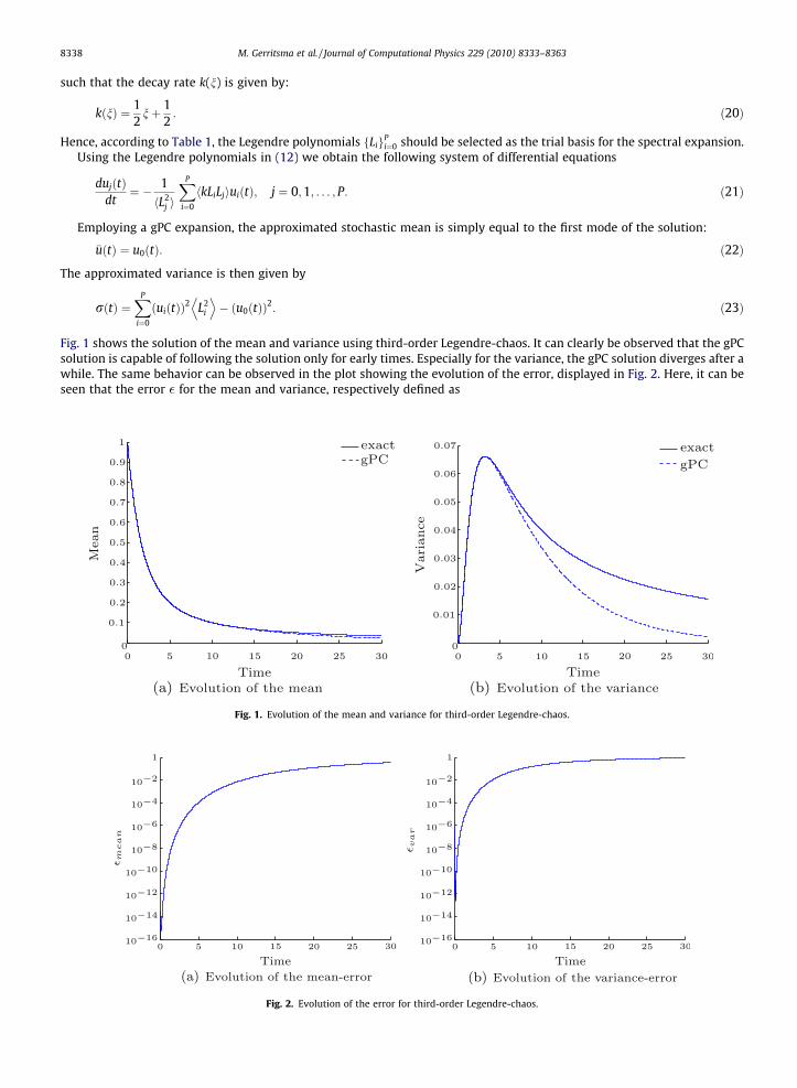
Fig. 1 shows the solution of the mean and variance using third-order Legendre-chaos. It can clearly be observed that the gPCsolution is capable of following the solution only for early times. Especially for the variance, the gPC solution diverges after awhile. The same behavior can be observed in the plot showing the evolution of the error, displayed in Fig. 2. Here, it can beseen that the error � for the mean and variance, respectively defined as

Fig. 1. Evolution of the mean and variance for third-order Legendre-chaos.

Fig. 2. Evolution of the error for third-order Legendre-chaos.

Fig. 3. Behavior of the variance for increasing order Legendre-chaos.

Fig. 4. Error convergence of the mean and variance.


�meanðtÞ ¼�uðtÞ � �uexactðtÞ

�uexactðtÞ

��; �varðtÞ ¼

rðtÞ � rexactðtÞrexactðtÞ

�� ð24Þ

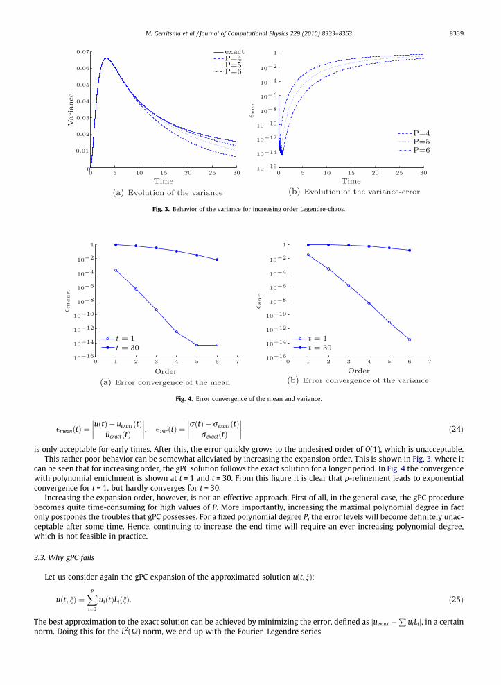
is only acceptable for early times. After this, the error quickly grows to the undesired order of O(1), which is unacceptable.This rather poor behavior can be somewhat alleviated by increasing the expansion order. This is shown in Fig. 3, where it

can be seen that for increasing order, the gPC solution follows the exact solution for a longer period. In Fig. 4 the convergencewith polynomial enrichment is shown at t = 1 and t = 30. From this figure it is clear that p-refinement leads to exponentialconvergence for t = 1, but hardly converges for t = 30.

Increasing the expansion order, however, is not an effective approach. First of all, in the general case, the gPC procedurebecomes quite time-consuming for high values of P. More importantly, increasing the maximal polynomial degree in factonly postpones the troubles that gPC possesses. For a fixed polynomial degree P, the error levels will become definitely unac-ceptable after some time. Hence, continuing to increase the end-time will require an ever-increasing polynomial degree,which is not feasible in practice.

3.3. Why gPC fails

Let us consider again the gPC expansion of the approximated solution u(t,n):

uðt; nÞ ¼XP

i¼0

uiðtÞLiðnÞ: ð25Þ

The best approximation to the exact solution can be achieved by minimizing the error, defined as juexact �P

uiLij, in a certainnorm. Doing this for the L2(X) norm, we end up with the Fourier–Legendre series


uðt; nÞ ¼XP

i¼0

aiðtÞLiðnÞ; ð26Þ

in which the Legendre coefficients ai(t) are given by:

aiðtÞ ¼huexactLii

L2i

D E ð27Þ

with the ensemble average h�,�i defined as in (6). More explicitly, it can be calculated that the Legendre coefficients for thestochastic ODE problem in question, are given by:

aiðtÞ ¼Xi

j¼0

1tjþ1

ðiþ jÞ!ði� jÞ!j! ðð�1Þiþj � e�tÞ: ð28Þ

The only error occurring in the finite Fourier–Legendre series approximation is due to truncation. In fact, it is the optimal Pthorder approximation, being the interpolant of the exact solution.

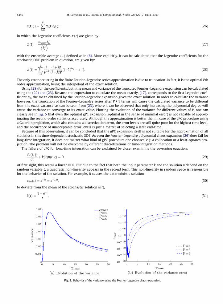
Using (28) for the coefficients, both the mean and variance of the truncated Fourier–Legendre expansion can be calculatedusing the (22) and (23). Because the expression to calculate the mean exactly, (17), corresponds to the first Legendre coef-ficient a0, the mean obtained by the Fourier–Legendre expansion gives the exact solution. In order to calculate the variancehowever, the truncation of the Fourier–Legendre series after P + 1 terms will cause the calculated variance to be differentfrom the exact variance, as can be seen from (23), where it can be observed that only increasing the polynomial degree willcause the variance to converge to its exact value. Plotting the evolution of the variance for different values of P, one canclearly see in Fig. 5 that even the optimal gPC expansion (optimal in the sense of minimal error) is not capable of approx-imating the second-order statistics accurately. Although the approximation is better than in case of the gPC procedure usinga Galerkin projection, which also contains a discretization error, the error levels are still quite poor for the highest time level,and the occurrence of unacceptable error levels is just a matter of selecting a later end-time.

Because of this observation, it can be concluded that the gPC expansion itself is not suitable for the approximation of allstatistics in this time-dependent stochastic ODE. As even the Fourier–Legendre polynomial chaos expansion (26) does fail forlong-time integration, it does not matter what kind of gPC procedure one chooses, e.g. a collocation or a least-squares pro-jection. The problem will not be overcome by different discretizations or time-integration methods.

The failure of gPC for long-time integration can be explained by closer examining the governing equation:

duðt; nÞdt

þ kðnÞuðt; nÞ ¼ 0: ð29Þ

At first sight, this seems a linear ODE. But due to the fact that both the input parameter k and the solution u depend on therandom variable n, a quadratic non-linearity appears in the second term. This non-linearity in random space is responsiblefor the behavior of the solution. For example, it causes the deterministic solution

udetðtÞ ¼ e��kt ¼ e�0:5t; ð30Þ

to deviate from the mean of the stochastic solution �uðtÞ,

�uðtÞ ¼ 1� e�t

t; ð31Þ

Fig. 5. Behavior of the variance using the Fourier–Legendre chaos expansion.


i.e. the deterministic solution employing the most probable value �k of the input parameter k

�k ¼ E½k� ¼Z 1

0kfk dk ¼ 1

2; ð32Þ

does not correspond to the mean of the stochastic solution, incorporating the range and distribution of the random param-eter k. In Fig. 6, it can be clearly seen that only for early times, those values do correspond, while for increasing time, thedifference grows. This behavior is known as stochastic drift. This implies that only for early times, the solution can be approx-imated as a linear continuation of the random input. For increasing time, the non-linear development becomes more andmore dominant, requiring an increasing amount of terms in the polynomial chaos expansion in terms of the input expansion.A way to see this, is to consider that the solution remembers and resembles the stochastic input only for early times, whilefor later times, the solution starts to deviate from the distribution of the input due to the occurring quadratic non-linearityand starts to develop its own stochastic characteristics. As a result, for longer time integration, expressing the solution interms of the input parameter requires more and more expansion terms. As for the Gaussian inputs discussed in Section 2,the appearance of the higher-order modes in the expansion indicates that the solution is drifting away from a uniformly dis-tributed stochastic process and therefore the concept of optimal polynomial chaos as explained in [5] will no longer be appli-cable. The failure observed for gPC is not limited to gPC. Probabilistic Collocation methods show a similar behaviour. Thebehaviour of PCM and additional considerations for long-time integration are given in Appendix A.

3.4. Time-dependent Wiener–Hermite expansion

An alternative approach of expanding random variables is in terms of so-called ideal random functions [25]. Ideal randomfunctions are improper functions which can be interpreted as the derivative of the Wiener random function.

The expansion in terms of ideal random functions also breaks down for time-dependent problems. In [26–28] it was pro-posed to make the random functions time-dependent and to set up a separate differential equation for the determination ofthe optimal time-dependent ideal random functions. In [27] it is stated that: ‘‘The principle idea of the method is to choosedifferent ideal random functions at different times in such a way that the unknown random function is expressed with good approx-imation by the first few terms of the Wiener–Hermite expansion for long-time duration. As an example it will be shown in I that theexactly Gaussian solutions of turbulence in an incompressible inviscid fluid and the three-mode problem are expressed by the firstterm alone of the Wiener–Hermite expansion if we take a suitable time-dependent ideal random function as the variable.”

The assumption is that for different times t, different random functions A(x, t) = H(1)(x, t) should be chosen (see [25, Eq.(3.2)] for the definition of the functions HðnÞi1 ;...;in

ðxÞ). Assuming that the ‘‘new” random functions are not too different fromthe ‘‘old” random functions, they can be approximated by a rapidly converging Wiener–Hermite expansion in time, whichgives the differential equation from which the new random functions can be obtained. The coefficients in the evolution equa-tion are constrained by the fact that the new random functions should satisfy the properties of ideal random functions [25,Eqs. (2.1) and (2.2)].

In the current paper the same basic idea is employed, namely that the basis functions in which the random variable isexpanded should change as a function of time, but no separate evolution equation is set up for the new basis functions. In-stead, the solution at a given time t is chosen as the new random variable and the ‘‘old” basis functions are now expressed interms of this ‘‘new” random variable.

3.5. Time-dependent polynomial chaos

In this section the basic idea, as developed by Vos [29], of time-dependent generalized polynomial chaos will be ex-plained. This idea is easy to understand and fully reflects the notion that the PDF changes as function of time and therefore

Fig. 6. Evolution of deterministic solution and the mean of the stochastic solution.


requires a different set of orthogonal polynomials. In the next section the same approach will be applied to the Kraichnan–Orszag three-mode problem and there several improvements on this basic idea will be presented.

Time-dependent polynomial chaos works as follows. Consider the same ODE problem as in Section 3.1

duðt; nÞdt

þ kðnÞuðt; nÞ ¼ 0: ð33Þ

We start with the gPC procedure using a Legendre-chaos expansion as explained in Section 3.2

uðt; nÞ ¼XP

i¼0

uiðtÞLiðnÞ: ð34Þ

As this gPC approach works fine for early times, this is a suitable approach to start with. However, when progressing in timeusing an RK4 numerical integration, the results start to become worse due to the quadratic non-linearity in random space.That is why at a certain time level, the gPC procedure should be stopped, preferably before the non-linear development be-comes too significant. This can be monitored by inspecting the non-linear terms in the gPC expansion of the solution. Con-sequently, stopping the numerical integration in time when the non-linear coefficients become too big with respect to thelinear coefficient, given by the condition

maxðju2ðtÞj; . . . ; juPðtÞjÞPju1ðtÞj

h; ð35Þ

can be used as a suitable stopping criterion.Suppose we halt the gPC procedure at t = t1. We now change the expansion by introducing a new random variable equal to

the solution u at t = t1, given by

w ¼ uðt1; nÞ ¼XP

i¼0

uiðt1ÞLiðnÞ ¼ TðnÞ; ð36Þ

where T maps n onto w. This mapping is not necessarily bijective. If the PDF of n is given by fn(n), then the PDF of w can inprinciple be obtained from, [30,31]

fwðwÞ ¼X

n

fnðnnÞdTðnÞ

dn

��n¼nn

��; ð37Þ

where the sum is taken so as to include all the roots nn, n = 1,2, . . . which are the real solutions of the equation
w ¼ TðnÞ ¼ 0: ð38Þ
The new gPC expansion should be a polynomial expansion in terms of this random variable w. According to the gPC rules, thepolynomial basis {Ui} should be chosen such that the polynomials are orthogonal with respect to a weighting function equalto the PDF of w. Because the random variable w depends on the solution, the new polynomial basis should be created on-the-fly. Having obtained the new PDF in terms of w we can set up a system of monic orthogonal polynomials with respect to theweight function fw(w). This orthogonal system is defined by

/0ðwÞ ¼ 1;Z/iðwÞ/jðwÞfwðwÞdw ¼ cidij; i; j ¼ 1; . . . ; P:

ð39Þ

As mentioned before, various alternatives are feasible to create this set of polynomials numerically. In this work, we chooseto create the orthogonal polynomial basis using a Gram–Schmidt orthogonalization. In this way, a new proper gPC expansionof the solution will be created. With respect to this new orthogonal system the solution u can be represented as

uðt;wÞ ¼XP

i¼0

uiðtÞ/iðwÞ: ð40Þ

Moreover, because it is based on the statistics of the solution, it is the optimal gPC expansion which will yield optimal con-vergence for early times, starting from t = t1.

However, before the gPC procedure can be continued, some extra information should be updated. First of all, the solutionat time level t1, uðt1; nÞ ¼

Puiðt1ÞLiðnÞ, should be translated to new (stochastic) initial conditions for u in terms of the new

random variable w. Due to the use of monic orthogonal polynomials in the Gram–Schmidt orthogonalization, this yields thefollowing exact expansion

uðt1;wÞ ¼ /1ðwÞ � u0ðt1Þ/0ðwÞ; ð41Þ
in which u0(t1) is equal to the value of u0(t1) from the old expansion. Note that this is a linear expansion in w.
In practice, the new PDF (37), is not explicitly constructed, but we make use of the mapping (36)
ZgðwÞfwdw ¼
ZgðTðnÞÞfndn ð42Þ

to convert all integrals to the original stochastic variable n.


This new expansion should then be employed until a next time level t2, at which criterion (35) is fulfilled again. Then, thealgorithm should be repeated. In this way, one can march through the time domain, reinitializing the gPC expansion at cer-tain discrete time levels. The whole idea of transforming the problem to a different random variable at those time levels is tocapture the non-linearity of the problem under consideration in the PDF. The time-dependent generalized polynomial chaoscan be summarized as:

Algorithm

– construct an ODE system employing gPC based on the random input– integrate in time– time step i: if maxðju2ðtiÞj; . . . ; juPðtiÞjÞP ju1ðtiÞj

h

– calculate the PDF of wnew

– Gram–Schmidt orthogonalization: create a random trial basis {Ui(wnew)}– generate new initial conditions: u(ti,wprev) ? u(ti,wnew)– construct a new ODE system using (42)– calculate mean and variance– postprocessing

The rationale behind TDgPC is the idea that the coefficient k and the solution u need not have the same probability dis-tribution. We assume that the solution of the decay model can be decomposed as

uðt; fÞ ¼XN

i¼0

uiðtÞ/iðfÞ; ð43Þ

where the basis functions /i(f) are orthogonal with respect to the probability density function fu(t,f) of u and not the probabilitydensity function fk(n) of the stochastically distributed decay coefficient k(n). Then the expansion coefficients are given by

ujðtÞ ¼1

/2j

D E Z 1

�1uðt; fÞ/jðfÞfuðt; fÞdf; ð44Þ

and hence,

duj

dt¼ 1

/2j

D E Z 1

�1

@uðt; fÞ@t

/jðfÞfuðt; fÞdfþ 1

/2j

D E Z 1

�1uðt; fÞ/jðfÞ

@fuðt; fÞ@t

df

¼ �1

/2j

D E Z 1

�1kðnÞuðt; fÞ/jðfÞfuðt; fÞdfþ 1

/2j

D E Z 1

�1uðt; fÞ/jðfÞ

@fuðt; fÞ@t

df

¼ �1

/2j

D E XN

i¼0

uiðtÞZ 1

�1kðnÞ/iðfÞ/jðfÞfuðt; fÞdfþ 1

/2j

D E XN

i¼0

uiðtÞZ 1

�1/iðfÞ/jðfÞ

@fuðt; fÞ@t

df:

The problem with this approach is twofold

1. How is f related to n?2. How can we determine the time derivative @fu/ot in the second term on the right hand side?

We know that the distribution of u is related to the distribution of k. Once we fix k, we have a deterministic solution, so let usmake f a function of n, i.e. f = f(n), then we have for the coefficientsZ

ujðtÞ ¼1

/2j

D E 1

�1uðt; fÞ/jðfÞfuðt; fÞdf

¼ 1

/2j

D E Z 1

�1uðt; fðnÞÞ/jðfðnÞÞfuðt; fðnÞÞ

dfdn

dn

¼ 1

/2j

D E Z 1

�1uðt; fðnÞÞ/jðfðnÞÞfkðnÞdn:

If we now take the time derivative of uj(t) we obtain

duj

dt¼ 1

/2j

D E Z 1

�1

@uðt; fðnÞÞ@t

/jðfðnÞÞfkðnÞdn ¼ �1

/2j

D E Z 1

�1kðnÞuðt; fðnÞÞ/jðfðnÞÞfkðnÞdn

¼ �1

/2j

D E XN

i¼0

uiðtÞZ 1

�1kðnÞ/iðfðnÞÞ/jðfðnÞÞfkðnÞdn:

This we recognize as TDgPC, when we set f = u(t,n).


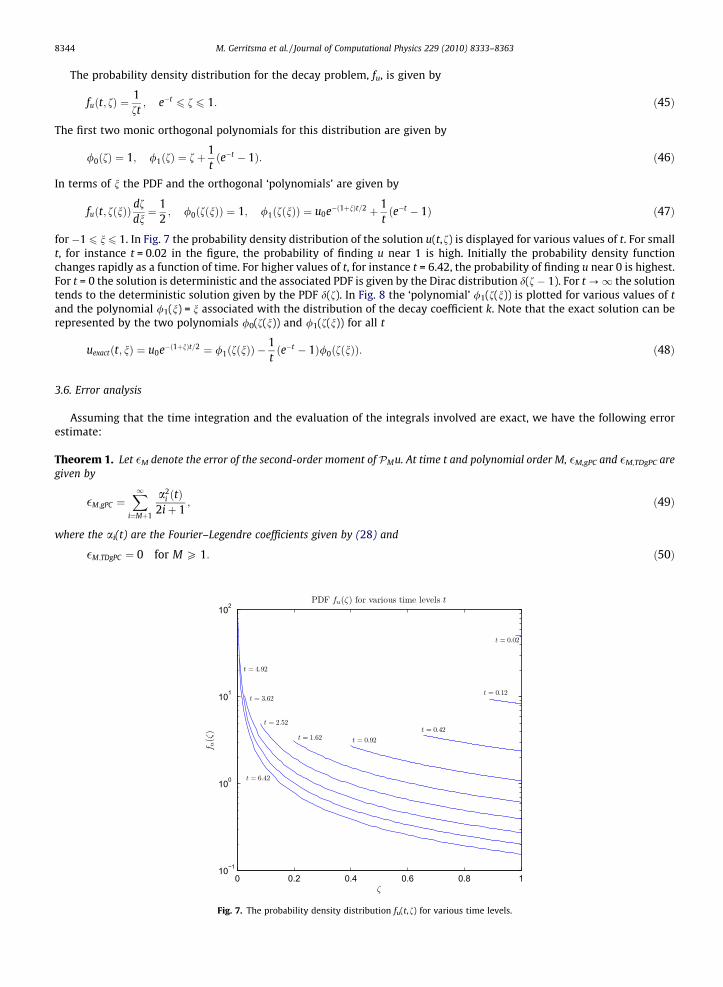
The probability density distribution for the decay problem, fu, is given by

fuðt; fÞ ¼1ft; e�t

6 f 6 1: ð45Þ

The first two monic orthogonal polynomials for this distribution are given by

/0ðfÞ ¼ 1; /1ðfÞ ¼ fþ 1tðe�t � 1Þ: ð46Þ

In terms of n the PDF and the orthogonal ‘polynomials’ are given by

fuðt; fðnÞÞdfdn¼ 1

2; /0ðfðnÞÞ ¼ 1; /1ðfðnÞÞ ¼ u0e�ð1þnÞt=2 þ 1

tðe�t � 1Þ ð47Þ

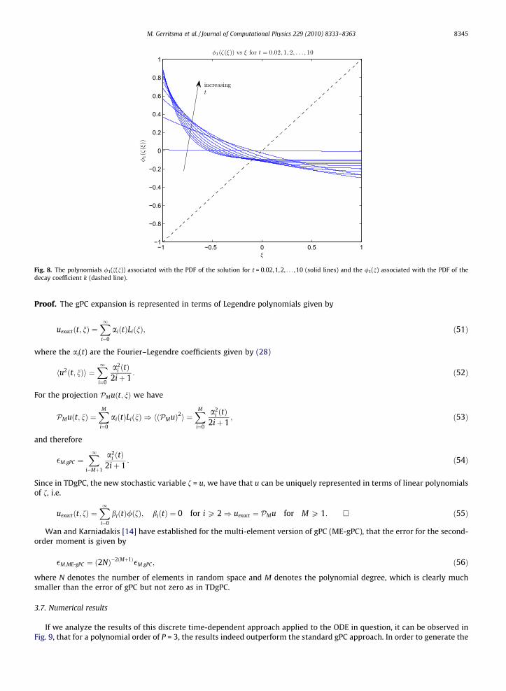
for �1 6 n 6 1. In Fig. 7 the probability density distribution of the solution u(t,f) is displayed for various values of t. For smallt, for instance t = 0.02 in the figure, the probability of finding u near 1 is high. Initially the probability density functionchanges rapidly as a function of time. For higher values of t, for instance t = 6.42, the probability of finding u near 0 is highest.For t = 0 the solution is deterministic and the associated PDF is given by the Dirac distribution d(f � 1). For t ?1 the solutiontends to the deterministic solution given by the PDF d(f). In Fig. 8 the ‘polynomial’ /1(f(n)) is plotted for various values of tand the polynomial /1(n) = n associated with the distribution of the decay coefficient k. Note that the exact solution can berepresented by the two polynomials /0(f(n)) and /1(f(n)) for all t

uexactðt; nÞ ¼ u0e�ð1þnÞt=2 ¼ /1ðfðnÞÞ �1tðe�t � 1Þ/0ðfðnÞÞ: ð48Þ

3.6. Error analysis

Assuming that the time integration and the evaluation of the integrals involved are exact, we have the following errorestimate:

Theorem 1. Let �M denote the error of the second-order moment of PMu. At time t and polynomial order M, �M,gPC and �M,TDgPC aregiven by

�M;gPC ¼X1

i¼Mþ1

a2i ðtÞ

2iþ 1; ð49Þ

where the ai(t) are the Fourier–Legendre coefficients given by (28) and

�M;TDgPC ¼ 0 for M P 1: ð50Þ

Fig. 7. The probability density distribution fu(t,f) for various time levels.

Fig. 8. The polynomials /1(f(n)) associated with the PDF of the solution for t = 0.02,1,2, . . . ,10 (solid lines) and the /1(n) associated with the PDF of thedecay coefficient k (dashed line).


Proof. The gPC expansion is represented in terms of Legendre polynomials given by

uexactðt; nÞ ¼X1i¼0

aiðtÞLiðnÞ; ð51Þ

where the ai(t) are the Fourier–Legendre coefficients given by (28)

hu2ðt; nÞi ¼X1i¼0

a2i ðtÞ

2iþ 1: ð52Þ

For the projection PMuðt; nÞ we have

PMuðt; nÞ ¼XM

i¼0

aiðtÞLiðnÞ ) hðPMuÞ2i ¼XM

i¼0

a2i ðtÞ

2iþ 1; ð53Þ

and therefore

�M;gPC ¼X1

i¼Mþ1

a2i ðtÞ

2iþ 1: ð54Þ

Since in TDgPC, the new stochastic variable f = u, we have that u can be uniquely represented in terms of linear polynomialsof f, i.e.

uexactðt; fÞ ¼X1i¼0

biðtÞ/ðfÞ; biðtÞ ¼ 0 for i P 2) uexact ¼ PMu for M P 1: � ð55Þ

Wan and Karniadakis [14] have established for the multi-element version of gPC (ME-gPC), that the error for the second-order moment is given by

�M;ME-gPC ¼ ð2NÞ�2ðMþ1Þ�M;gPC ; ð56Þ

where N denotes the number of elements in random space and M denotes the polynomial degree, which is clearly muchsmaller than the error of gPC but not zero as in TDgPC.

3.7. Numerical results

If we analyze the results of this discrete time-dependent approach applied to the ODE in question, it can be observed inFig. 9, that for a polynomial order of P = 3, the results indeed outperform the standard gPC approach. In order to generate the

Fig. 9. Evolution of the mean and variance for third-order time-dependent gPC (P = 3).


results, the threshold parameter was set equal to h = 6. Especially for the second-order statistics, which were a bottleneck forthe standard gPC, the improvement is significant. The same behavior can be seen from Fig. 10, displaying the evolution of theerror of both the mean and variance. Although the initial error level cannot be maintained, at the end-time, we see that boththe error-levels have dropped from an unacceptable order O(1) to the acceptable level O(10�2). The accuracy can be im-proved by increasing the polynomial degree P. As from a polynomial degree of P = 4, in a plot depicting the evolution themean and variance analogous to Fig. 9, the time-dependent gPC approximation would be indistinguishable from the exactsolution. In Fig. 11, the error evolution of mean and variance are depicted for different expansion orders.

Fig. 12 shows that the time-dependent TDgPC approach is more accurate than conventional gPC, but it also shows thatconvergence with polynomial enrichment is much slower than gPC. In fact, gPC is more accurate with respect to the meanthan TDgPC for higher polynomial orders. The lack of convergence is explained by the distribution of the decay coefficientk(n) = (1 + n)/2 for �1 6 n 6 1, which in terms of f is given by (�1/t) � lnf for exp(�t) 6 f 6 1. For large t this implies thatwe need to find a polynomial approximation in f to lnf for f 2 (0,1],

ln f ¼X1i¼0

aifi; e�t

6 f 6 1: ð57Þ

Since lnf R L2(0,1) we know that this expansion does not converge in the L2-norm for higher values of t, see Fig. 13.Or put differently, the transformation to the f-variables allows one to represent the solution at each time level exactly

with linear functions in f, as stated by Theorem 1, but is not adequate to describe the time rate of change of the solution.We therefore expand the solution in terms of f and n as

uðt; nÞ ¼XP

i¼0

XQ

j¼0

aijðtÞ/iðfÞLjðnÞ; ð58Þ

Fig. 10. Evolution of the error for third-order time-dependent gPC (P = 3).

Fig. 11. Evolution of the error for polynomial order P = 3, . . . ,6 for time-dependent gPC.

Fig. 12. Error convergence of the mean and variance at t = 30.


where the /i(f) constitute a set of orthogonal polynomials with respect to PDF of the solution, as discussed in this section andthe Lj(n) constitute an orthogonal set of polynomials with respect to the PDF of the decay coefficient k(n), i.e. the Legendrepolynomials. So for P = Q = 1, the expanion is given by

uðt; nÞ ¼ a00ðtÞ þ a01ðtÞnþ a1;0ðtÞ/1ðfðnÞÞ þ a11ðtÞn/1ðfðnÞÞ: ð59Þ

At time t = tn the solution is given by

aijðtnÞ ¼1 if i ¼ 1 and j ¼ 00 elsewhere

�ð60Þ

The time rate of change of the solution is given by

dudt¼ �1

2ð1þ nÞu ¼

XP

i;j

bijðtÞ/iðfÞLjðnÞ ) bijðtnÞ ¼�1=2 if i ¼ 1 and j ¼ 0;10 elsewhere

�ð61Þ

So with this expansion, both the solution and the time derivative can be fully represented. The number of terms required inthe expansion depends on the time-integration method employed. For Euler integration P = 1 and Q = 1 suffices and the errorin the approximation is dominated by time integration, since for the Euler scheme we have:

uðt þ Dt; nÞ ¼ uðt; nÞ � Dt2ð1þ nÞfðnÞ ð62Þ

For a fourth-order Runge–Kutta scheme a polynomial degree P = 4 and Q = 1 suffices, because for the Runge–Kutta schemewe have

Fig. 13. Natural logarithm and its sixth order approximation for t = 1, t = 10, t = 100 (left to right).

0 20 40 60 80 10010−16

10−15

10−14

10−13

10−12

10−11

t

rela

tive

erro

r

Ralative error in mean vs time

0 20 40 60 80 10010−16

10−14

10−12

10−10

10−8

10−6

t

rela

tive

erro

r

Relative error in variance vs time

Fig. 14. Evolution of the error for fifth-order time-dependent gPC for 0 6 t 6 100 integrated with a fourth order Runge–Kutta scheme in time, Dt = 0.001.

0 20 40 60 80 10010−16

10−14

10−12

10−10

10−8

10−6Relative error in the mean vs time

Rel

ativ

e er

ror m

ean

0 20 40 60 80 10010−13

10−12

10−11

10−10

10−9

10−8

10−7

10−6

10−5Relative error in variance vs time

Rel

ativ

e er

ror v

aria

nce

Fig. 15. Evolution of the error for P = 2 in the revised time-dependent gPC for 0 6 t 6 100.


0 20 40 60 80 10010−16

10−15

10−14

10−13

10−12

10−11

10−10Relative error in the mean vs time

Rel

ativ

e er

ror m

ean

0 20 40 60 80 10010−15

10−14

10−13

10−12

10−11

10−10

10−9

10−8

10−7

10−6

Rel

ativ

e er

ror v

aria

nce

Relative error in variance vs time

Fig. 16. Evolution of the error for P = 3 in the revised time-dependent gPC for 0 6 t 6 100.


uðt þ Dt; nÞ ¼ uðt; nÞ � Dt2ð1þ nÞfðnÞ þ Dt2

8ð1þ nÞ2fðnÞ � Dt3

48ð1þ nÞ3fðnÞ þ Dt4

384ð1þ nÞ4fðnÞ: ð63Þ

Fig. 14 shows the error as a function of time for this approach.

Corollary 2. The expansion of the random variable in orthogonal polynomials should be capable of representing the statistics ateach time level (Theorem 1) and should be capable of representing the time derivative. For the decay problem we have that if P isgreater or equal than the order of the time-integration scheme, the accuracy is determined by the accuracy of the time-integrationscheme. If P is less than the order of the time-integration scheme the accuracy is determined by DtP, because in that case the higher-order terms cannot be represented by polynomials in n. This is illustrated numerically for the fourth-order Runge–Kutta schemewith Dt = 0.001 for P = 2 and P = 3, in Figs. 15 and 16, respectively. For P = 2 this yields an error in the mean and the variance ofO(10�6) and for P = 3 an error in the mean and the variance of O(10�9) over the entire time interval.

Based on these observation, we now consider the more challenging case consisting of a system of ordinary non-linear dif-ferential equations.

4. The Kraichnan–Orszag three-mode problem

The so-called Kraichnan–Orszag three-mode problem was introduced by Kraichnan [2] and studied by Orszag [3] forGuassian distributed initial conditions.

4.1. Problem definition

The Kraichnan–Orszag problem is defined by the following system of non-linear ordinary differential equations

dx1

dt¼ x2x3; ð64aÞ

dx2

dt¼ x3x1; ð64bÞ

dx3

dt¼ �2x1x2: ð64cÞ

In this work we will consider this problem subject to stochastic initial conditions. First, we will study the 1D problem cor-responding to initial conditions of the form

x1ð0Þ ¼ aþ 0:01n; x2ð0Þ ¼ 1:0; x3ð0Þ ¼ 1:0; ð65Þ

where a is a constant and n a uniformly distributed random variable with unit variance (i.e. n is uniformly distributed on theinterval [�1,1]). Analysis by [16,32,33] shows that when a is in the range (0,0.9) the solution is rather insensitive to the ini-tial conditions. However for a 2 (0.9,1) there is a strong dependence on the initial conditions.

In Section 4.4 we will consider the 3D case


x1ð0Þ ¼ aþ 0:01n1; x2ð0Þ ¼ bþ 0:01n2; x3ð0Þ ¼ cþ 0:01n3; ð66Þ

where a, b and c are constants and n1, n2 and n3 are uniformly distributed random variables on the interval [�1,1], where n1,n2 and n3 are statistically independent.

4.2. TDgPC solution

Consider the Kraichnan–Orszag problem (64) with the initial conditions (65). We follow the procedure described in Sec-tion 3.5

xiðt; nÞ ¼XP

p¼0

xðiÞp ðtÞLpðnÞ; i ¼ 1;2;3; ð67Þ

where Lp is the Legendre polynomial of degree p. Since n has a uniform distribution, the Legendre polynomials constitute anoptimal trial basis for early times (see Table 1). Employing this polynomial chaos expansion of the solution and following themethod outlined in Section 2.2 we arrive at a system of deterministic ordinary differential equations in time for the coeffi-cients xðiÞp ðtÞ. We solve this system by standard fourth-order Runge–Kutta time integration.

From (67) we see that the approximate solutions xi are polynomials in the random variable n. With time the coefficients ofthe solution polynomials increase in magnitude. This is an indication that the stochastic characteristics of the solution arechanging. As a consequence the basis {Lp} looses its effectiveness. When the non-linear part of the solution reaches a certainthreshold level (say at t = t1), we perform the transformation of the random variable from n to fi given by

fi ¼ xiðt1; nÞ ¼XP

p¼0

xðiÞp ðt1ÞLpðnÞ; i ¼ 1;2;3: ð68Þ

The three new random variables fi have associated PDFs ffiðfiÞ.

For each ffiwe employ Gram–Schmidt orthogonalization to calculate a set of orthogonal polynomials /ðfiÞ

p ðfiÞ withp = 0, . . . ,P. By /ðfiÞ

p we denote the polynomial of degree p associated with ffi, i.e. ffi

acts as the weighting function in theorthogonality relation. At time level t = t1 these polynomials constitute an optimal trial basis again. We therefore use thesenewly calculated polynomials /ðfiÞ

p and continue to obtain a numerical solution to the Kraichnan–Orszag problem in a newform given by

xiðt; f1; f2; f3Þ ¼X

06lþmþn6P

xðiÞlmnðtÞ/ðf1Þl ðf1Þ/ðf2Þ

m ðf2Þ/ðf3Þn ðf3Þ; t P t1: ð69Þ

The summation in Eq. (69) is over all combinations of the integers l, m and n for which 0 6 l + m + n 6 P. The total number ofexpansion terms (N + 1) follows from Eq. (11) with n = 3 and is given by

N þ 1 ¼P þ 3

P

� �¼ ðP þ 3Þ!

P!3!¼ 1

6ðP þ 3ÞðP þ 2ÞðP þ 1Þ � P3

6: ð70Þ

Substituting (69) in (64) we once again follow the standard gPC procedure of Section 2.2. Hence, we perform a Galerkinprojection to end up with a new system of ordinary differential equations for the new expansion coefficients xðiÞlmnðtÞ.

We proceed by marching this new system forward in time again from t = t1 onwards using our standard fourth-order Run-ge–Kutta solver. Note, however, that we need to provide ‘initial’ conditions (i.e. conditions at t = t1) for all new coefficientsxðiÞlmn. These initial conditions follow from the requirement

xiðt1; f1; f2; f3Þ ¼ fi; i ¼ 1;2;3: ð71Þ

We can arrange for the orthogonal expansion polynomials /ðfiÞp to all have unity leading coefficients. Therefore, at t = t1 the

coefficients xðiÞlmn are given by

xð1Þlmnðt1Þ ¼�/ðf1Þ

0 if l ¼ m ¼ n ¼ 0;1 if l ¼ 1 ^m ¼ n ¼ 0;0 otherwise;

8><>:


0 if l ¼ m ¼ n ¼ 0;1 if m ¼ 1 ^ l ¼ n ¼ 0;0 otherwise;

8><>:


0 if l ¼ m ¼ n ¼ 0;1 if n ¼ 1 ^ l ¼ m ¼ 0;0 otherwise;

8><>:

ð72Þ

where /ðfiÞ0 denotes the zeroth-order term of the expansion polynomial of degree one associated with ffi

.


Marching the new system of differential equations forward in time, we again monitor the non-linear part of the resultingsolution. When, by some criterion, this non-linear part has become too large (say at t = t2), we repeat the above procedure inorder to re-establish an optimal trial basis. Hence, we start by introducing the new random variables

fð2Þi ¼ xi t2; fð1Þ1 ; fð1Þ2 ; fð1Þ3

� ; i ¼ 1;2;3; ð73Þ

and continue to calculate their PDFs from which the new optimal trial basis is calculated by Gram–Schmidt orthogonaliza-tion. Note that we have added a superscript to the random variables in (73) corresponding to the time instant at which theywere introduced. Hence, we have rewritten the original variables fi as fð1Þi . The process of updating the polynomial trial basiscan be performed as many times as is required for the particular problem at hand. So, in general we have

fðkþ1Þi ¼ xi tkþ1; f

ðkÞ1 ; fðkÞ2 ; fðkÞ3

� ; i ¼ 1;2;3; k ¼ 1;2; . . . ;K � 1 ð74Þ �

with associated PDF ffðkþ1Þ

iand orthogonal polynomials /

fðkþ1Þi

p leading to a polynomial chaos expansion, similar to (69), to beused for tk+1 6 t 6 tk+2.

4.2.1. System of differential equations after a random variable transformationHaving made the transformation (68) from the single initial random variable n to the three new random variables fi – note

that we have dropped the superscript (1) again for clarity – we approximate the solution to the 1D Kraichnan–Orszag prob-lem by (69). When we substitute this expression into (64a) we obtain

X06iþjþk6P

dxð1Þijk

dt/ðf1Þ

i /ðf2Þj /ðf3Þ

k ¼X

06pþqþr6P

X06uþvþw6P

xð2Þpqrxð3Þuvw/ðf1Þ

p /ðf2Þq /ðf3Þ

r /ðf1Þu /ðf2Þ

v /ðf3Þw : ð75Þ

We multiply this equation by /ðf1Þl ff1 /

ðf2Þm ff2 /

ðf3Þn ff3 and perform a triple integration w.r.t. f1, f2 and f3. Taking into account the

orthogonality of the basis functions, we arrive at

dxð1Þlmn

dt¼ 1

/ðf1Þl

2D E/ðf2Þ

m2

D E/ðf3Þ

n2

D E X06pþqþr6P

X06uþvþw6P

xð2Þpqrxð3Þuvw /ðf1Þ

p /ðf1Þu /ðf1Þ

l

D E/ðf2Þ

q /ðf2Þv /ðf2Þ

m

D E/ðf3Þ

r /ðf3Þw /ðf3Þ

n

D Eð76Þ

for l, m, n = 0, . . . ,P with

hIðfiÞi ¼Z 1

�1IðfiÞffi

ðfiÞdfi ð77Þ

for some function I(fi). Substituting (69) into (64b) and (64c) gives similar relations as (76) for the evolution of xð2Þlmn and xð3Þlmn.Together these three equations constitute the governing deterministic system of differential equations in time for the expan-sion coefficients xðiÞlmnðtÞ, i = 1,2,3 with 0 6 l + m + n 6 P.

4.2.2. Calculation of mean and varianceWe are interested in the mean and variance of x1 (t,f1,f2,f3), x2(t,f1,f2,f3) and x3(t,f1,f2,f3). Once we have solved for the

time histories of the solution coefficients xðiÞlmnðtÞ (see (69)) the mean and variance of xi (t,f1,f2,f3) can be calculated as follows.Mean The mean of xi is defined as

�xiðtÞ ¼ E½xiðt; f1; f2; f3Þ�: ð78Þ

Substituting Eq. (69) into Eq. (78) we get

�xiðtÞ ¼ EX

06lþmþn6P

xðiÞlmnðtÞ/ðf1Þl ðf1Þ/ðf2Þ

m ðf2Þ/ðf3Þn ðf3Þ

" #

¼Z 1

�1

Z 1

�1

Z 1

�1

X06lþmþn6P

xðiÞlmnðtÞ/ðf1Þl / f2ð Þ

m /ðf3Þn ff1 ;f2 ;f3 df1 df2 df3: ð79Þ

If f1, f2 and f3 were statistically independent, this could be reduced to three one-dimensional integrals, using

ff1 ;f2 ;f3 ðf1; f2; f3Þ ¼ ff1 ðf1Þff2 ðf2Þff3 ðf3Þ: ð80Þ

However, this will not be the case, since the stochastic variables fi are all related by various mappings to the common sto-chastic variables n.

Variance. The variance of xi is defined as

VarðxiðtÞÞ ¼ E½ðxiðt; f1; f2; f3Þ � �xiðtÞÞ2� ¼ E x2i ðt; f1; f2; f3Þ � 2xiðt; f1; f2; f3Þ�xiðtÞ þ �x2

i ðtÞ�

¼ E x2i ðt; f1; f2; f3Þ

� � 2E xiðt; f1; f2; f3Þ½ ��xiðtÞ þ �x2

i ðtÞ ¼ E x2i ðt; f1; f2; f3Þ

� � �x2

i ðtÞ: ð81Þ

Substituting the numerical approximation ((69) and (79) into (81) we obtain


VarðxiðtÞÞ ¼ EX

06lþmþn6P

xðiÞlmnðtÞ/ðf1Þl /ðf2Þ

m /ðf3Þn

!224

35� xðiÞ000

2ðtÞ

¼Z 1

�1

Z 1

�1

Z 1

�1

X06lþmþn6P


m /ðf3Þn

!2

ff1 ;f2 ;f3 df1 df2 df3: ð82Þ

4.2.3. Integration over the original random variableThe integrand in (82) for the variance, for instance, of xi is a function of the transformed random variables f1, f2 and f3.

These transformed random variables, in turn, are all functions of the original random variable n: f1 = Z1(n), f2 = Z2(n) andf3 = Z3(n). Hence, the integrand in (82) can also be seen as a function solely dependent on n. To avoid the calculation offf1 ;f2 ;f3 we can transform the triple integral over f1, f2 and f3 in (82) to a single integral over n, based on the ideas fromVan der Steen [32].

We do this by recognizing that the following relation should be valid for every realisable point f�1; f�2; f

�3

�
ff1 ;f2 ;f3 f�1; f
�2; f

�3

�df1 df2 df3 ¼

Xn�

fnðn�Þdn; ð83Þ

where the summation is over all points n* for which Z1ðn�Þ ¼ f�1; Z2ðn�Þ ¼ f�2 and Z3ðn�Þ ¼ f�3. Eq. (83) merely states that, giventhe transformation n ? (f1,f2,f3), the probability that (f1,f2,f3) lies within an infinitesimal volume around f�1; f

�2; f

�3

�should

be equal to the probability that n lies within the (possibly multiple) corresponding infinitesimal interval(s) around n*. It fol-lows that the following relation should then also be valid
Z 1
�1

Z 1

�1

Z 1

�1� � � ff1 ;f2 ;f3 df1 df2 df3 ¼

Z 1

�1� � � fn dn: ð84Þ

Hence, with the help of (84) we can calculate the variance of xi according to

VarðxiðtÞÞ ¼ EX

06lþmþn6P


m /ðf3Þn

!224

35� �x2

i ðtÞ

¼Z 1

�1

Z 1

�1

Z 1

�1

X06lþmþn6P


m /ðf3Þn

!2

ff1 ;f2 ;f3 df1 df2 df3 � �x2i ðtÞ

¼Z 1

�1

X06lþmþn6P

xðiÞlmnðtÞ/ðf1Þl ðZ1ðnÞÞ/ðf2Þ

m ðZ2ðnÞÞ/ðf3Þn ðZ3ðnÞÞ

!2

fnðnÞdn� �x2i ðtÞ: ð85Þ

Transforming an integral over the transformed random variables to an integral over the original random variable is atechnique that can be used to evaluate the mean, i.e.

�xiðtÞ ¼Z 1

�1

Z 1

�1

Z 1

�1

X06lþmþn6P


m /ðf3Þn ff1 ;f2 ;f3 df1 df2 df3

¼X

06lþmþn6P

xðiÞlmnðtÞZ 1

�1/ðf1Þ

l ðZ1ðnÞÞ/ðf2Þm ðZ2ðnÞÞ/ðf3Þ

n ðZ3ðnÞÞfnðnÞdn: ð86Þ

Furthermore, we can just as well transform a single integral over a transformed random variable to a single integral overthe original random variable. So, similarly to (83), we also have that

ffif�i �

dfi ¼Xn�

fnðn�Þdn; ð87Þ

so
Z 1
�1� � � ffi

dfi ¼Z 1

�1� � � fn dn: ð88Þ

With the help of (88) we can transform all integrals needed for the determination of the governing system of differentialequations ((76) and (77)) to integrals over the original random variable n. The integrals in the Gram–Schmidt orthogonali-zation algorithm (to calculate the orthogonal polynomials /ðfiÞ

p ðfiÞ) can similarly be transformed to integrals over n.To conclude, we make the following important point. Performing all integrations in n-space has a major advantage: there

is no need to explicitly calculate the probability density functions of the transformed random variables as was done in (37).

4.3. Numerical results

Figs. 17 and 18 show results for the mean and variance for x1, calculated using the TDgPC solution approach where atransformation to new stochastic variables is performed every time step. Similar results are obtained for x2 and x3. At approx-

t

Mean(x 1)

0 10 20 30 40-1

-0.5

0

0.5

1TDgPC P = 2TDgPC P = 3MC N = 200,000

Fig. 17. Mean of x1 vs. time for a = 0.99: TDgPC solutions with P = 2 and P = 3 compared to Monte-Carlo analysis (N = 200,000).

t

Var(x

1)

0 10 20 30 400

0.1

0.2

0.3

0.4

0.5

0.6

TDgPC P = 2TDgPC P = 3MC N = 200,000

Fig. 18. The variance of x1 vs. time for a = 0.99: TDgPC solutions with P = 2 and P = 3 compared to Monte-Carlo analysis (N = 200,000).


imately t = 13, the results generated with the gPC solution stop to bear any resemblance to the Monte-Carlo solution. How-ever, using a TDgPC strategy with expansion polynomials having a maximum degree of only two (P = 2) shows a significantimprovement. The calculated solution can be seen to have the same characteristics as the results from the Monte-Carlo anal-ysis for the entire range of t displayed. Increasing the maximum degree of the expansion polynomials to P = 3 leads to resultswith even higher accuracy. In fact, the TDgPC results with P = 3 are graphically indistinguishable from the Monte-Carlo re-sults on the scale of these plots.

t

ε mean(x1)

0 10 20 30 40

-0.04

-0.02

0

0.02

0.04P = 2P = 3P = 4

t

ε var(x1)

0 10 20 30 40-0.04

-0.02

0

0.02

0.04

P = 2P = 3P = 4

Fig. 19. Error in the mean and variance of x1 vs. time for a = 0.99: TDgPC solutions with P = 2, P = 3 and P = 4.


In Fig. 19 the time evolution of the ‘error’ in the mean and variance, respectively, of x1 is shown for various values of P.Here ‘error’ means the difference between the TDgPC results and a Monte Carlo analysis with 200,000 samples

Mean(x)

Fig. 20analysi

��xiðtÞ ¼ �xTDgPC

i ðtÞ � �xMCi ðtÞ: ð89Þ

The error in the variance is calculated similarly. The error plots more clearly show the accuracy we gain by going from P = 2to P = 3. The accuracy of a TDgPC solution with P = 4 can be seen to be almost identical to a solution with P = 3. Using Cor-ollary 2 we can show that for P = 2, the method is O(Dt), which for Dt = 0.001 is O(10�3), for P = 3, the method isO(Dt2) = O(10�6) and for P = 4 O(Dt3) = O(10�9). If we use the expansion given by (75) we can represent the solution at eachtime step. For P = 2, we can also represent quadratic terms and therefore we can represent

x1ðt þ D; nÞ ¼ x1ðt; nÞ þ Dtf2f3; ð90Þx2ðt þ D; nÞ ¼ x2ðt; nÞ þ Dtf3f1; ð91Þ

and

x3ðt þ D; nÞ ¼ x3ðt; nÞ � 2Dtf1f2: ð92Þ

So for P = 2, we have a method that is first order in time. For P = 3, we can also represent all the cubic terms in f1, f2 and f3

multiplied by Dt2 in the Runge–Kutta integration. So for P = 3 we have a second-order method in time. Analogously, we canshow that for P = 4, we can represent all terms up to the power of 4 in fi with coefficient D t3. Now the difference between anerror of 10�6 and 10�9 are visually undistinguishable in Fig. 19. It has been confirmed that this error cannot be attributed to

t

1

0 10 20 30 40

-0.5

0

0.5

1 TDgPC P = 2TDgPC P = 3gPC P = 10MC N = 100,000

t

Var(x

1)

0 10 20 30 400

0.1

0.2

0.3

0.4

0.5

0.6

0.7

TDgPC P = 2TDgPC P = 3gPC P = 10MC N = 100,000

. Mean and variance of x1 vs. time for a = 0.995: TDgPC solutions with P = 2 and P = 3 compared to a gPC solution with P = 10 and a Monte-Carlos (N = 100,000).

t

ε mean(x1)

0 10 20 30 40-0.06

-0.04

-0.02

0

0.02

0.04

P = 2P = 3

t

ε var(x1)

0 10 20 30 40

-0.02

0

0.02

0.04

P = 2P = 3

Fig. 21. Error in the mean and variance of x1 vs. time for a = 0.995: TDgPC solutions with P = 2 and P = 3.


the integration method and therefore the difference observed between the TdgPC results and the Monte-Carlo result must beattributed to number of samples in the Monte-Carlo simulation.

4.3.1. Results for a = 0.995Here we investigate the performance of TDgPC results for a = 0.995 in (65). This is an interesting case, because for

x1(0) < 1 we have periodic solutions. The period becomes strongly dependent on x1(0) > 0.9. When x1(0) > 1 the solutioncurves belong to a different branch of solution trajectories than for x1(0) < 1. The chance of finding an initial condition suchthat x1(0) > 1, is P(x1(0) > 1) = 0.25, so this choice of a contains two significantly different types of solutions. Furthermore, theperiods T of the periodic solution near x1(0) = 1 are very sensitive to the initial conditions. See, for instance [16,32], for moredetails on the dynamics of the Kraichnan–Orszag problem.

In Fig. 20 TDgPC results are presented for the mean (a) and variance (b) of x1. We again compare the TDgPC solutions withresults from a Monte-Carlo simulation. Also for a = 0.995 TDgPC remains close to the Monte-Carlo results. The accuracy ofthe solution with P = 2 is comparable to the case a = 0.99. Again there is a significant improvement going from P = 2 toP = 3. However, the solution for P = 3 is not quite as accurate as in the case a = 0.99. This is presumably due to the highercomplexity of the problem with a = 0.995. In Fig. 21 the ‘error’ in the mean and variance are plotted for x1, respectively, tak-ing the Monte-Carlo simulation with N = 100,000 as a reference.

4.4. A three-dimensional random space

In this case we show a result where all three initial conditions are known with a given probability. These initial conditionsare given by (also considered in [16])

Mean(x)

Fig. 22.analysi

x1ð0Þ ¼ aþ 0:01n1; x2ð0Þ ¼ bþ 0:01n2; x3ð0Þ ¼ cþ 0:01n3; ð93Þ

where a, b and c are constants and n1, n2 and n3 are uniformly distributed random variables on the interval [�1,1] where n1,n2 and n3 are statistically independent. Here we set a = 0.99, b = 1 and c = 1.

We now start with a three-dimensional expansion in terms of n1, n2 and n3 analogous to (69). We introduce transformedrandom variables according to (74) and calculate new expansion polynomials similarly to the single random variable case.We also transform all integrals occurring in the solution algorithm to integrals over the original independent random vari-ables n1, n2 and n3. Since we now have three original random variables instead of one (83) is rewritten as

ff1 ;f2 ;f3 f�1; f�2; f

�3

�df1 df2 df3 ¼

Xn�1 ;n

�2 ;n�3ð Þ

fn1 ;n2 ;n3 n�1; n�2; n

�3

�dn1 dn2 dn3 ¼

Xn�1 ;n

�2 ;n�3ð Þ

fn1 n�1 �

fn2 n�2 �

fn3 n�3 �

dn1 dn2 dn3 ð94Þ

for every realisable point f�1; f�2; f

�3

�. The summation in (94) is over all points n�1; n

�2; n

�3

�for which Z1 n�1; n

�2; n

�3

�¼

f�1; Z2 n�1; n�2; n

�3

�¼ f�2 and Z3 n�1; n

�2; n

�3

�¼ f�3. Note that in (94) we have made use of the statistical independence of n1, n2

and n3 in the initial conditions. It follows from (94) that integrals over the new random variables can be transformed accord-ing to
Z 1
�1

Z 1

�1

Z 1

�1� � � ff1 ;f2 ;f3 df1 df2 df3 ¼

Z 1

�1

Z 1

�1

Z 1

�1� � � fn1 fn2 fn3 dn1 dn2 dn3: ð95Þ

t

1

0 10 20 30 40

-0.5

0

0.5

1

TDgPC P = 2TDgPC P = 3gPC P = 2MC N = 1,000,000

t

Var(x

1)

0 10 20 30 400

0.2

0.4

TDgPC P = 2TDgPC P = 3gPC P = 2MC N = 1,000,000

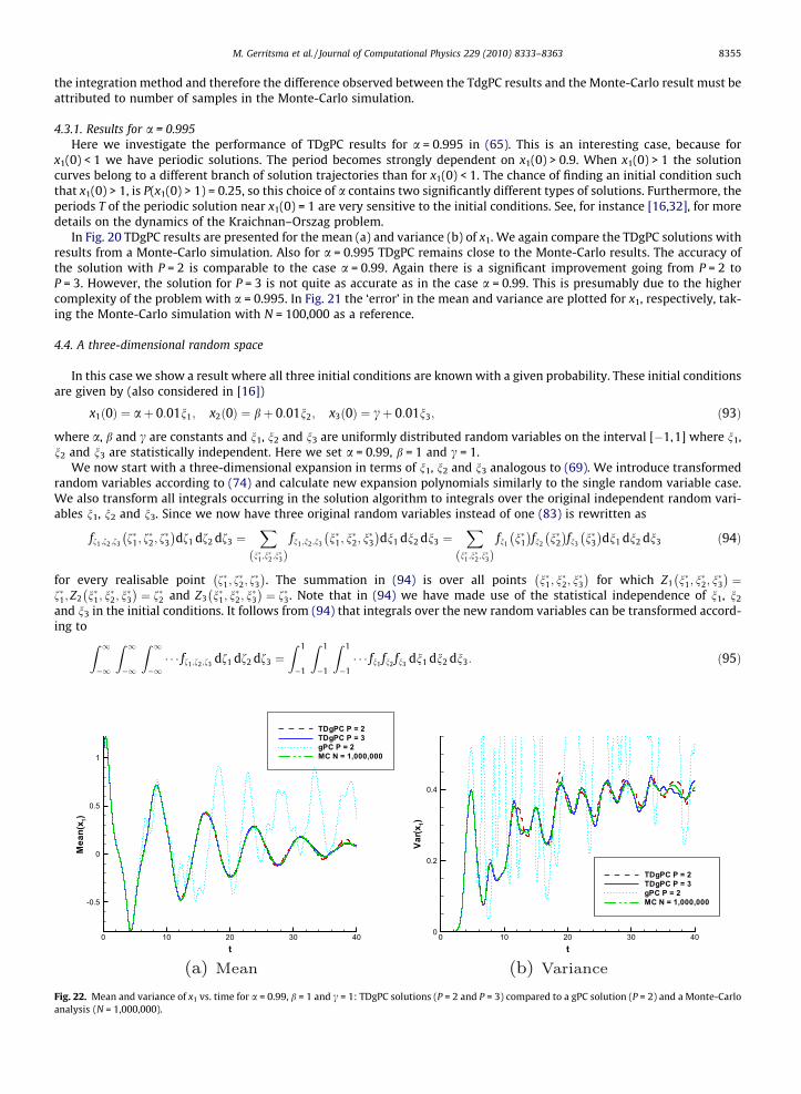
Mean and variance of x1 vs. time for a = 0.99, b = 1 and c = 1: TDgPC solutions (P = 2 and P = 3) compared to a gPC solution (P = 2) and a Monte-Carlos (N = 1,000,000).


Unlike the single random variable case we still have to deal with a three-dimensional integral after transformation. We cantreat this integral as a repeated one-dimensional integral, since n1, n2 and n3 are statistically independent.

4.4.1. ResultsIn Fig. 22 we compare the results from a TDgPC solution approach to gPC results and a Monte-Carlo analysis. We choose

values of P = 2 and P = 3 for the two TDgPC solutions in this comparison. From approximately t = 12 onwards the gPC resultsfor the mean of x1 lose any resemblance to the correct solution. When looking at the variance of x1 this point is alreadyreached at t = 4.

The TDgPC results with P = 2 remain reasonably close to the Monte Carlo analysis results for the entire time interval con-sidered, although the curves can be seen to lose some of their accuracy as time progresses. Increasing P from P = 2 to P = 3results in an increase in accuracy: TDgPC results for the mean of x1 are now visually indistinguishable from the Monte-Carloresults for the entire time interval displayed. The accuracy of the variance of x1 goes up as well, but the TDgPC curve is notprecisely on top of the Monte-Carlo curve as was the case for a one-dimensional random input. A comparison of TDgPC, gPCand Monte-Carlo results for x2 and x3 shows similar characteristics as the results for x1.

5. Conclusions

In this paper an adaptive gPC method in time is proposed, the time-dependent generalized polynomial chaos (TDgPC).TDgPC takes into account that the probability density function (PDF) of the solution changes as a function of time. Due tothis change in PDF, orthogonal polynomials that were optimal initially, loose their optimality for increasing time and anew set of orthogonal polynomials needs to be created. The method has been applied to a simple decay model and theKraichnan–Orszag three-mode problem. In the latter case both the situation with one random initial condition and threerandom initial conditions were considered. Based on computational results TDgPC ameliorates the accuracy when usinglong-time integration. The advantage of this approach is that the polynomial degree can be kept low (P = 2, 3 or 4) withoutintroducing multiple elements (ME-gPC, [16]) in random space. This leads in the cases considered to a reduction of the num-ber of degrees of freedom and consequently to a reduction in the number of deterministic problems that need to be solved.The additional cost is the construction of new sets of orthogonal polynomials (which for P 3 is quite cheap) and the integraltransformations in setting up the deterministic equations and the calculation of the statistical moments.

Whether gPC type methods are the preferred way of solving stochastic differential equations is beyond the scope of thispaper. This generally depends on practical issues like the size of the problem, the availability of deterministic solvers, thenumber of stochastic variables in the problem and the required accuracy.

Current research focuses on the application of TDgPC to partial differential equations. Future directions for research in-clude the combination of TDgPC with ME-gPC, where in each element new stochastic variables are introduced. This will leadto a very effective and efficient algorithm, especially for solutions with low regularity such as the Kraichnan–Orszag problemcorresponding to a = 0.995. Furthermore, the new polynomials associated with the PDF of the solution, introduced in thispaper, may lead to improved collocation points for the multi-element probabilistic collocation method ME-PCM, [34].

Acknowledgments

The authors wish to thank Joris Oostelbos for providing some of the figures. Professor Karniadakis wishes to acknowledgethe financial support from OSD/AFOSR MURI.

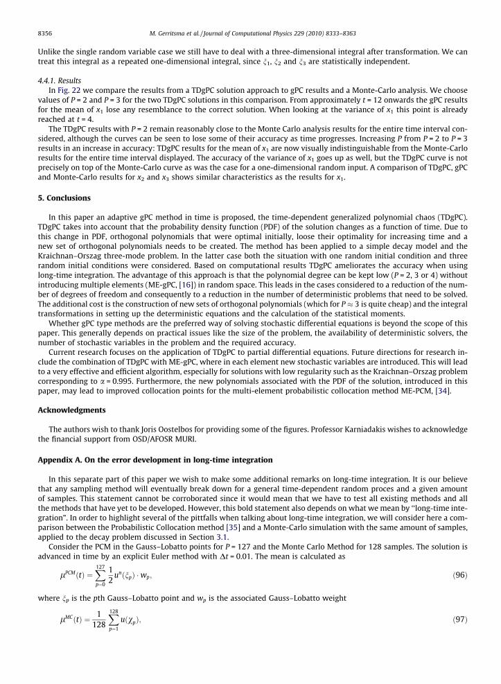
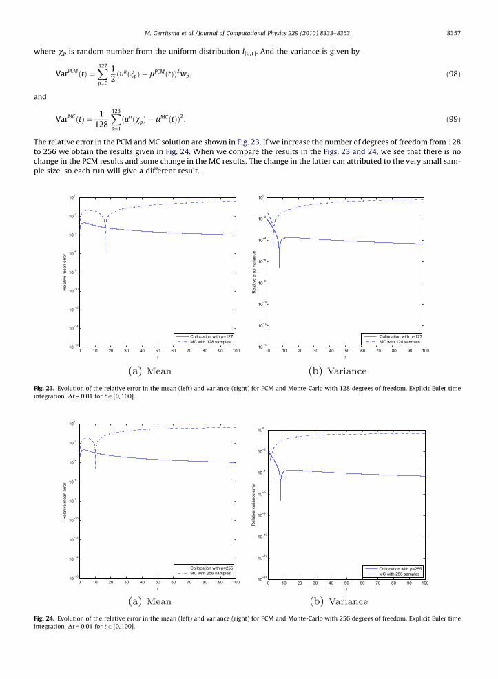
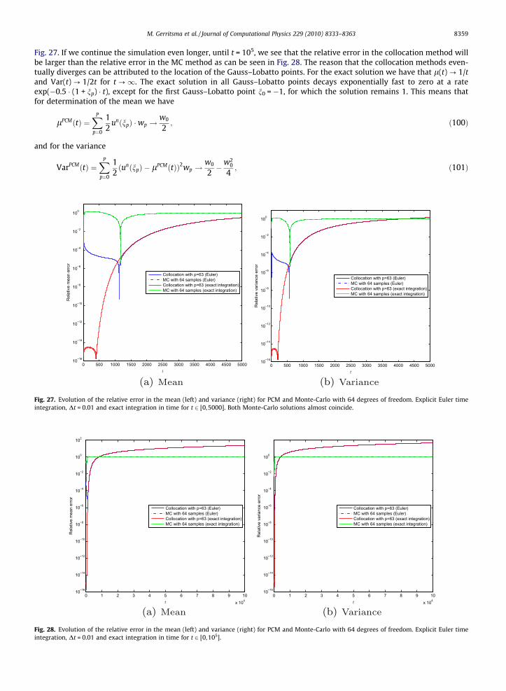
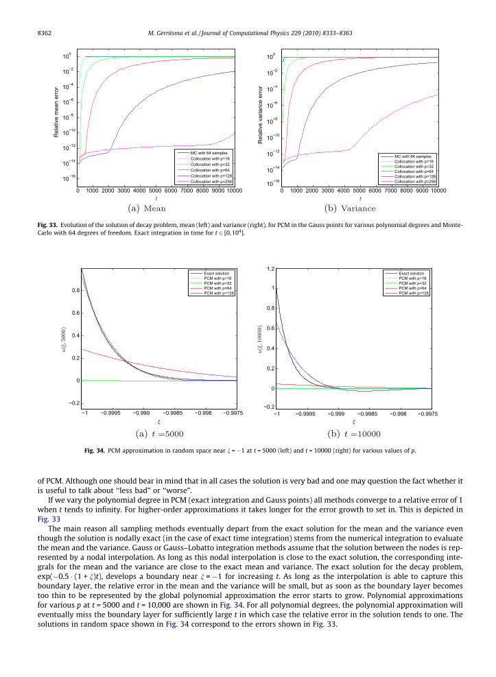
Appendix A. On the error development in long-time integration

In this separate part of this paper we wish to make some additional remarks on long-time integration. It is our believethat any sampling method will eventually break down for a general time-dependent random proces and a given amountof samples. This statement cannot be corroborated since it would mean that we have to test all existing methods and allthe methods that have yet to be developed. However, this bold statement also depends on what we mean by ‘‘long-time inte-gration”. In order to highlight several of the pittfalls when talking about long-time integration, we will consider here a com-parison between the Probabilistic Collocation method [35] and a Monte-Carlo simulation with the same amount of samples,applied to the decay problem discussed in Section 3.1.

Consider the PCM in the Gauss–Lobatto points for P = 127 and the Monte Carlo Method for 128 samples. The solution isadvanced in time by an explicit Euler method with Dt = 0.01. The mean is calculated as

lPCMðtÞ ¼X127

p¼0

12

unðnpÞ �wp; ð96Þ

where np is the pth Gauss–Lobatto point and wp is the associated Gauss–Lobatto weight

lMCðtÞ ¼ 1128

X128

p¼1

uðvpÞ; ð97Þ


where vp is random number from the uniform distribution I[0,1]. And the variance is given by

Fig. 23.integra

Fig. 24.integra

VarPCMðtÞ ¼X127

p¼0

12ðunðnpÞ � lPCMðtÞÞ2wp; ð98Þ

and

VarMCðtÞ ¼ 1128

X128

p¼1

ðunðvpÞ � lMCðtÞÞ2: ð99Þ

The relative error in the PCM and MC solution are shown in Fig. 23. If we increase the number of degrees of freedom from 128to 256 we obtain the results given in Fig. 24. When we compare the results in the Figs. 23 and 24, we see that there is nochange in the PCM results and some change in the MC results. The change in the latter can attributed to the very small sam-ple size, so each run will give a different result.

0 10 20 30 40 50 60 70 80 90 10010−16

10−14

10−12

10−10

10−8

10−6

10−4

10−2

100

Rel

ativ

e m

ean

erro

r

Collocation with p=127MC with 128 samples

0 10 20 30 40 50 60 70 80 90 10010−14

10−12

10−10

10−8

10−6

10−4

10−2

100

Rel

ativ

e er

ror v

aria

nce


Evolution of the relative error in the mean (left) and variance (right) for PCM and Monte-Carlo with 128 degrees of freedom. Explicit Euler timetion, Dt = 0.01 for t 2 [0,100].

0 10 20 30 40 50 60 70 80 90 10010−16

10−14

10−12

10−10

10−8

10−6

10−4

10−2

100

Rel

ativ

e m

ean

erro

r


0 10 20 30 40 50 60 70 80 90 10010−14

10−12

10−10

10−8

10−6

10−4

10−2

100

Rel

ativ

e va

rianc

e er

ror


Evolution of the relative error in the mean (left) and variance (right) for PCM and Monte-Carlo with 256 degrees of freedom. Explicit Euler timetion, Dt = 0.01 for t 2 [0,100].


For a proper assessment of the error in time-dependent calculations we need to be able to decompose the error due to thetime integration and the error due to sampling in random space. Since there is hardly any change when the sample size isdoubled, it is tempting to attribute the error to the time integration. In order to investigate this, we run these two test casesagain, but this time we use exact integration instead of the explicit Euler method. The results of this exercise can be found inFigs. 25 and 26.

From these figures we see that the relative error in the collocation method can be attributed to the time integration; theerror drops to machine accuracy when exact integration is used instead of numerical integration. The relative error in the MCmethod is dominated by the error in random space; the two solutions with numerical integration and exact time integrationare almost indistinguishable.

From these observations one may conclude that the collocation method provides a more accurate description in randomspace compared to the MC method. This conclusion is justified for this particular problem and this particular time interval.

If we run the same test case for a longer period, i.e. until t = 5000 instead of t = 100 we see that the error in random spacegrows and starts to dominate the relative errors in the mean and variance at t 1200 and t 500, respectively, as shown in

0 10 20 30 40 50 60 70 80 90 10010−16

10−14

10−12

10−10

10−8

10−6

10−4

10−2

100

Rel

ativ

e m

ean

erro

r

Collocation with p=127 (Euler)MC with 128 samples (Euler)Collocation with p=127 (exact integration)MC with 128 samples (exact integration)

0 10 20 30 40 50 60 70 80 90 10010−16

10−14

10−12

10−10

10−8

10−6

10−4

10−2

100

Rel

ativ

e va

rianc

e er

ror

PCM with p=127 (Euler)MC with 128 samples (Euler)PCM with p=127 (exact integration)MC with 128 samples (exact integration)

Fig. 25. Evolution of the relative error in the mean (left) and variance (right) for PCM and Monte-Carlo with 128 degrees of freedom. Explicit Euler timeintegration, Dt = 0.01 and exact integration in time for t 2 [0, 100].

0 10 20 30 40 50 60 70 80 90 10010−16

10−14

10−12

10−10

10−8

10−6

10−4

10−2

100

Rel

ativ

e m

ean

erro

r


(a) Mean

0 10 20 30 40 50 60 70 80 90 10010−16

10−14

10−12

10−10

10−8

10−6

10−4

10−2

100

Rel

ativ

e va

rianc

e er

ror


(b) Variance

Fig. 26. Evolution of the relative error in the mean (left) and variance (right) for PCM and Monte-Carlo with 256 degrees of freedom. Explicit Euler timeintegration, Dt = 0.01 and exact integration in time for t 2 [0, 100].


Fig. 27. If we continue the simulation even longer, until t = 105, we see that the relative error in the collocation method willbe larger than the relative error in the MC method as can be seen in Fig. 28. The reason that the collocation methods even-tually diverges can be attributed to the location of the Gauss–Lobatto points. For the exact solution we have that l(t) ? 1/tand Var(t) ? 1/2t for t ?1. The exact solution in all Gauss–Lobatto points decays exponentially fast to zero at a rateexp(�0.5 � (1 + np) � t), except for the first Gauss–Lobatto point n0 = �1, for which the solution remains 1. This means thatfor determination of the mean we have

Fig. 27.integra

Fig. 28.integra

lPCMðtÞ ¼XP

p¼0

12

unðnpÞ �wp !w0

2; ð100Þ

and for the variance

VarPCMðtÞ ¼XP

p¼0

12ðunðnpÞ � lPCMðtÞÞ2wp !

w0

2�w2

0

4; ð101Þ

0 500 1000 1500 2000 2500 3000 3500 4000 4500 500010−16

10−14

10−12

10−10

10−8

10−6

10−4

10−2

100

Rel

ativ

e m

ean

erro

r


0 500 1000 1500 2000 2500 3000 3500 4000 4500 500010−16

10−14

10−12

10−10

10−8

10−6

10−4

10−2

100

Rel

ativ

e va

rianc

e er

ror


Evolution of the relative error in the mean (left) and variance (right) for PCM and Monte-Carlo with 64 degrees of freedom. Explicit Euler timetion, Dt = 0.01 and exact integration in time for t 2 [0,5000]. Both Monte-Carlo solutions almost coincide.

0 1 2 3 4 5 6 7 8 9 10x 104

10−16

10−14

10−12

10−10

10−8

10−6

10−4

10−2

100

102

Rel

ativ

e m

ean

erro

r


0 1 2 3 4 5 6 7 8 9 10x 104

10−16

10−14

10−12

10−10

10−8

10−6

10−4

10−2

100

Rel

ativ

e va

rianc

e er

ror


Evolution of the relative error in the mean (left) and variance (right) for PCM and Monte-Carlo with 64 degrees of freedom. Explicit Euler timetion, Dt = 0.01 and exact integration in time for t 2 [0,105].


For the relative error in mean and variance this means that

Fig. 29.Dt = 0.0

Fig. 30integra

rel: mean error ¼ w0

2t þ const and rel: variance error ¼ w0 �

w20

2

� �t þ const: ð102Þ

This linear growth is shown in Fig. 29. In Table 2 the growth rates based on (102) are compared with the values obtainedfrom the calculation for P = 63 for which w0 = 4.9603 � 10�4 For the MC method a sample taken at the point n = �1 has prob-

0 1 2 3 4 5 6 7 8 9 10x 104

5

10

15

20

25

Rel

ativ

e m

ean

erro

r


0 1 2 3 4 5 6 7 8 9 10x 104

5

10

15

20

25

30

35

40

45

50

Rel

ativ

e va

rianc

e er

ror


Evolution of the relative error in the mean (left) and variance (right) for PCM and Monte-Carlo with 64 degrees of freedom. Exact time integration,1 and exact integration in time for t 2 [0,105].

Table 2Theoretical and experimental growth.

Theoretical slope Numerical slope

Mean 2.4802 � 10�4 2.4801 � 10�4

Variance 4.9591 � 10�4 4.9591 � 10�4

0 0.2 0.4 0.6 0.8 1 1.2 1.4 1.6 1.8 2x 104

10−100

10−90

10−80

10−70

10−60

10−50

10−40

10−30

10−20

10−10

100

Collocation with p=63 (Euler)Exact solutionMC with 64 samples (Euler)

0 0.2 0.4 0.6 0.8 1 1.2 1.4 1.6 1.8 2x 104

10−200

10−180

10−160

10−140

10−120

10−100

10−80

10−60

10−40

10−20

100

Collocation with p=63 (Euler)MC with 64 samples (Euler)Exact solution

. Evolution of the solution of the mean (left) and variance (right) for PCM and Monte-Carlo with 64 degrees of freedom. Explicit Euler timetion, Dt = 0.01 and exact integration in time for t 2 [0, 2 � 104].


ability zero, so we will not see linear growth in the relative error of the mean for the Monte-Carlo simulation. Since all solu-tion of the samples will decay to zero exponentially fast, the relative error in the mean and the Variance of the MC method,will converge to 1, which is confirmed by the simulation. In Fig. 30 the solution of the mean and variance are plotted on alogarithmic scale. We see that the absense of the point vp = �1 leads to solution which tend to zero too fast.

The growth is not associated with the fact that the mean and variance of the exact solution go to zero. If we solve theproblem

Fig. 31.Euler ti

Fig. 32.degrees

dudtþ kðnÞu ¼ 1

2; ð103Þ

the mean decays to a half and we see exactly the same long-time behaviour, see Fig. 31. The level of the relative mean error islower in this figure, due to the fact for large t we divide by 1/2 + C/t, instead of C/t, but we still observe linear growth for PCM.

If, instead of the Gauss–Lobatto nodes for the PCM method, we use the internal Gauss points and thereby exclude thedetrimental node n0 = �1, we observe that PCM and the MC method display a similar error evolution for t ?1, as can beseen in Fig. 32. So a judicious choice of integration points in the PCM method significantly affects the long-time behaviour

0 1000 2000 3000 4000 5000 6000 7000 8000 9000 1000010−16

10−14

10−12

10−10

10−8

10−6

10−4

10−2

100

Rel

ativ

e m

ean

erro

r


0 1000 2000 3000 4000 5000 6000 7000 8000 9000 1000010−16

10−14

10−12

10−10

10−8

10−6

10−4

10−2

100

Rel

ativ

e er

ror v

aria

nce


Evolution of the solution of the solution of (103), mean (left) and variance (right), for PCM and Monte-Carlo with 64 degrees of freedom. Explicitme integration, Dt = 0.01 and exact integration in time for t 2 [0, 104].

0 0.2 0.4 0.6 0.8 1 1.2 1.4 1.6 1.8 2x 104

10−16

10−14

10−12

10−10

10−8

10−6

10−4

10−2

100

Rel

ativ

e m

ean

erro

r

Collocation Gauss with p=128 (Euler)MC with 128 samples (Euler)Collocation Gauss with p=128 (exact integration)MC with 128 samples (exact integration)

0 0.2 0.4 0.6 0.8 1 1.2 1.4 1.6 1.8 2x 104

10−16

10−14

10−12

10−10

10−8

10−6

10−4

10−2

100

Rel

ativ

e va

rianc

e er

ror

Collocation Gauss with p=128 (Euler)MC with 128 samples (Euler)Collocation Gauss with p=128 (exact integration)MC with 128 samples (exact integration)

Evolution of the solution of the solution of decay problem, mean (left) and variance (right), for PCM in the Gauss points and Monte-Carlo with 128of freedom. Explicit Euler time integration, Dt = 0.01 and exact integration in time for t 2 [0,2 � 104].

0 1000 2000 3000 4000 5000 6000 7000 8000 9000 10000

10−16

10−14

10−12

10−10

10−8

10−6

10−4

10−2

100R

elat

ive

mea

n er

ror

MC with 64 samplesCollocation with p=16Collocation with p=32Collocation with p=64Collocation with p=128Collocation with p=256

0 1000 2000 3000 4000 5000 6000 7000 8000 9000 1000010−16

10−14

10−12

10−10

10−8

10−6

10−4

10−2

100

Rel

ativ

e va

rianc

e er

ror

MC with 64 samplesCollocation with p=16Collocation with p=32Collocation with p=64Collocation with p=128Collocation with p=256

Fig. 33. Evolution of the solution of decay problem, mean (left) and variance (right), for PCM in the Gauss points for various polynomial degrees and Monte-Carlo with 64 degrees of freedom. Exact integration in time for t 2 [0,104].

−1 −0.9995 −0.999 −0.9985 −0.998 −0.9975

−0.2

0

0.2

0.4

0.6

0.8

Exact solutionPCM with p=16PCM with p=32PCM with p=64PCM with p=128

−1 −0.9995 −0.999 −0.9985 −0.998 −0.9975−0.2

0

0.2

0.4

0.6

0.8

1

1.2Exact solutionPCM with p=16PCM with p=32PCM with p=64PCM with p=128

Fig. 34. PCM approximation in random space near n = �1 at t = 5000 (left) and t = 10000 (right) for various values of p.


of PCM. Although one should bear in mind that in all cases the solution is very bad and one may question the fact whether itis useful to talk about ‘‘less bad” or ‘‘worse”.

If we vary the polynomial degree in PCM (exact integration and Gauss points) all methods converge to a relative error of 1when t tends to infinity. For higher-order approximations it takes longer for the error growth to set in. This is depicted inFig. 33

The main reason all sampling methods eventually depart from the exact solution for the mean and the variance eventhough the solution is nodally exact (in the case of exact time integration) stems from the numerical integration to evaluatethe mean and the variance. Gauss or Gauss–Lobatto integration methods assume that the solution between the nodes is rep-resented by a nodal interpolation. As long as this nodal interpolation is close to the exact solution, the corresponding inte-grals for the mean and the variance are close to the exact mean and variance. The exact solution for the decay problem,exp(�0.5 � (1 + n)t), develops a boundary near n = �1 for increasing t. As long as the interpolation is able to capture thisboundary layer, the relative error in the mean and the variance will be small, but as soon as the boundary layer becomestoo thin to be represented by the global polynomial approximation the error starts to grow. Polynomial approximationsfor various p at t = 5000 and t = 10,000 are shown in Fig. 34. For all polynomial degrees, the polynomial approximation willeventually miss the boundary layer for sufficiently large t in which case the relative error in the solution tends to one. Thesolutions in random space shown in Fig. 34 correspond to the errors shown in Fig. 33.


References

[1] N. Wiener, The homogeneous chaos, American Journal of Mathematics 60 (4) (1938) 897–936.[2] R.H. Kraichnan, Direct-interaction approximation for a system of several interacting simple shear waves, The Physics of Fluids 6 (11) (1963) 1603–

1609.[3] S.A. Orszag, L.R. Bissonnette, Dynamical properties of truncated Wiener–Hermite expansions, The Physics of Fluids 10 (12) (1967) 2603–2613.[4] R.G. Ghanem, P.D. Spanos, Stochastic Finite Elements: A Spectral Approach, Springer-Verlag, New York, 1991.[5] D. Xiu, G. Karniadakis, The Wiener–Askey polynomial chaos for stochastic differential equations, SIAM Journal on Scientific Computing 24 (2) (2002)

619–644.[6] D. Xiu, G. Karniadakis, Modeling uncertainty in flow simulations via generalized polynomial chaos, Journal of Computational Physics 187 (1) (2003)

137–167.[7] B. Debusschere, H. Najm, A. Matta, O. Knio, R. Ghanem, O. Le Maître, Protein labeling reactions in electrochemical microchannel flow: Numerical

simulation and uncertainty propagation, Physics of Fluids 15 (2003) 2238–2250.[8] B.V. Asokan, N. Zabaras, Using stochastic analysis to capture unstable equilibrium in natural convection, Journal of Computational Physics 108 (2005)

134–153.[9] O.V. Knio, O. Le Maître, Uncertainty propagation in cfd using polynomial chaos decomposition, Fluid Dynamics Research 38 (2006) 614–640.

[10] O.P. Le Maître, M.T. Reagan, H.N. Najim, R.G. Ghanem, O.M. Knio, A stochastic projection method for fluid flow – II. Random process, Journal ofComputational Physics 181 (2002) 9–44.

[11] H.N. Najim, Uncertainty quantification and polynomial chaos techniques in computational fluid dynamics, Annual Review of Fluid Mechanics 41(2009) 35–52.

[12] X. Wan, G. Karniadakis, Beyond Wiener–Askey expansions: handling arbitrary PDFs, Journal of Scientific Computing 27 (1–3) (2006) 455–464.[13] C. Soize, R. Ghanem, Physical systems with random uncertainties: chaos representations with arbitrary probability measure, SIAM Journal of Scientific

Computing 26 (2) (2004) 395–410.[14] X. Wan, G. Karniadakis, Long-term behavior of polynomial chaos in stochastic flow simulations, Computer Methods in Applied Mechanics and

Engineering 195 (1–3) (2006) 5582–5596.[15] T.Y. Hou, W. Luo, B. Rozovskii, H.-M. Zhou, Wiener chaos expansions and numerical solutions of randomly forced equations of fluid mechanics, Journal

of Computational Physics 216 (2006) 687–706.[16] X. Wan, G. Karniadakis, An adaptive multi-element generalized polynomial chaos method for stochastic differential equations, Journal of

Computational Physics 209 (2) (2005) 617–642.[17] C.L. Pettit, P.S. Beran, Spectral and multiresolution Wiener expansions of oscillatory stochastic processes, Journal of Sound and Vibrations 294 (2006)

752–779.[18] J.A.S. Witteveen, H. Bijl, An alternative unsteady adaptive stochastic finite element formulation based on interpolation at constant phase, Computer

Methods in Applied Mechanics and Engineering 198 (2008) 578–591.[19] J.A.S. Witteveen, H. Bijl, Effect of randomness on multi-frequency aeroelastic response resolved by unsteady adaptive finite elements, Journal of

Computational Physics 228 (2009) 7025–7045.[20] J.A.S. Witteveen, H. Bijl, A TVD uncertainty quantification method with bounded error applied to transonic airfoil flutter, Communications in

Computational Physics 6 (2009) 406–432.[21] R.H. Cameron, W.T. Martin, The orthogonal development of non-linear functionals in series of Fourier–Hermite functionals, Annals of Mathematics 48

(2) (1947) 385–392.[22] H. Ogura, Orthogonal functionals of the Poisson process, IEEE Transactions on Information Theory 18 (4) (1972) 473–481.[23] J. Stoer, R. Bulirsch, Introduction to Numerical Analysis, Springer-Verlag, New York, 1979.[24] J.A.S. Witteveen, H. Bijl, Efficient quantification of the effect of uncertainties in advection–diffusion problems using polynomial chaos, Numerical Heat

Transfer B – Fundamental 53 (2008) 437–465.[25] T. Imamura, W.C. Meecham, A. Siegel, Symbolic calculus of the Wiener process and Wiener–Hermite functionals, Journal of Mathematical Physics 6 (5)

(1965) 695–706.[26] M. Doi, T. Imamura, The Wiener–Hermite expansion with time-dependent ideal random function, Progress of Theoretical Physics 41 (2) (1969) 358–

366.[27] S. Tanaka, T. Imamura, The Wiener–Hermite expansion with time-dependent ideal random function. II – The three-mode model, Progress of

Theoretical Physics 45 (4) (1971) 1098–1105.[28] M. Yano, T. Imamura, Time-dependent Wiener–Hermite expansion for the nearly Gaussian turbulence in the Burgers’ system, Physics of Fluids 15 (4)

(1972) 708–710.[29] P. Vos, Time-Dependent Polynomial Chaos, Master’s Thesis, Delft University of Technology, November 2006.[30] A.M. Mood, F.A. Graybill, D.C. Boes, Introduction to the Theory of Statistics, third ed., McGraw-Hill Series in Probability and Statistics, McGraw-Hill,

Singapore, 1974.[31] P.Z. Peebles, Probability, Random Variables, and Random Signal Principles, McGraw-Hill, New York, 1993.[32] J.B. Van der Steen, Time-Dependent Generalized Polynomial Chaos – Applied to the Kraichnan–Orszag Three-Mode Problem, Technical Report, Faculty

of Aerospace Engineering, TU Delft, 2008.[33] M. Gerritsma, P. Vos, J.-B. van der Steen, Time-dependent polynomial chaos, in: Theodore E. Simos, George Psihoyios, Ch. Tsitouras (Eds.), Numerical

Analysis and Applied Mathematics: International Conference on Numerical Analysis and Applied Mathematics 2008, Melville, NY, European Society ofComputational Methods in Sciences and Engineering, American Institute of Physics, 2008, pp. 221–224.

[34] J. Foo, X. Wan, G. Karniadakis, The multi-element probabilistic collocation method (ME-PCM): error analysis and applications, Journal ComputationalPhysics 227 (22) (2008) 9572–9595.

[35] J.R. Hockenberry, B.C. Lesieutre, Evaluation of uncertainty quantification of power system models: the probabilistic collocation method, IEEETransactions on Power Systems 19 (3) (2004) 1483–1491.

Date post:	04-Sep-2019
Category:	Documents
Upload:	others
View:	2 times
Download:	0 times

Journal of Computational Physics - Brown University · cFlemish Institute for Technological...

Documents