j ourna l homepage: www.e lsev ie r .com/ locate / jconhyd
Numerical study of wave effects on groundwater flow andsolute transport in a laboratory beach
Xiaolong Geng a, Michel C. Boufadel a,⁎, Yuqiang Xia b, Hailong Li c, Lin Zhao a,Nancy L. Jackson d, Richard S. Miller e
a Center for Natural Resources Development and Protection, Department of Civil and Environmental Engineering, New Jersey Institute of Technology, Newark, NJ 07102,United Statesb Changjiang River Scientific Research Institute (CRSRI), Changjiang Water Resources Commission of MWR, Wuhan 430010, Chinac School of Water Resources and Environmental Science, China University of Geoscience-Beijing, Beijing 100083, Chinad Department of Chemistry and Environmental Science, New Jersey Institute of Technology, Newark, NJ 07102, United Statese Department of Mechanical Engineering, Clemson University, Clemson, SC 29634-0921, United States
a r t i c l e i n f o
⁎ Corresponding author at: Center for Natural ResouProtection, New Jersey Institute of Technology, Newark
Article history:Received 14 January 2014Received in revised form 5 May 2014Accepted 1 July 2014Available online 8 July 2014
A numerical study was undertaken to investigate the effects of waves on groundwater flowand associated inland-released solute transport based on tracer experiments in a laboratorybeach. The MARUN model was used to simulate the density-dependent groundwater flow andsubsurface solute transport in the saturated and unsaturated regions of the beach subjected towaves. The Computational Fluid Dynamics (CFD) software, Fluent, was used to simulate waves,which were the seaward boundary condition for MARUN. A no-wave case was also simulatedfor comparison. Simulation results matched the observed water table and concentration atnumerous locations. The results revealed that waves generated seawater–groundwatercirculations in the swash and surf zones of the beach, which induced a large seawater–groundwater exchange across the beach face. In comparison to the no-wave case, wavessignificantly increased the residence time and spreading of inland-applied solutes in the beach.Waves also altered solute pathways and shifted the solute discharge zone further seaward.Residence Time Maps (RTM) revealed that the wave-induced residence time of theinland-applied solutes was largest near the solute exit zone to the sea. Sensitivity analysessuggested that the change in the permeability in the beach altered solute transport propertiesin a nonlinear way. Due to the slow movement of solutes in the unsaturated zone, the mass ofthe solute in the unsaturated zone, which reached up to 10% of the total mass in some cases,constituted a continuous slow release of solutes to the saturated zone of the beach. This meansof control was not addressed in prior studies.
In the last two decades, studies have revealed the ground-water system near the coastline is an important transportpathway for pollutants to enter the marine environment(Bakhtyar et al., 2012a; Boufadel et al., 2007; Moore, 1996;
rces Development and, NJ, United States.el).
Santas and Santas, 2000; Xin et al., 2010). The near-shoregroundwater system can be affected by many factors, such astides (Bobo et al., 2012; Guo et al., 2010), waves (Boufadel et al.,2007; Nielsen, 1999), pumping and climatic stresses (Alley et al.,2002; Calow et al., 1997). Gravity waves can affect beachgroundwater circulation patterns, and subsequently influencesolute transport in near-shore aquifers (Boufadel et al., 2007;Bradshaw, 1974; Horn et al., 1998). Understanding the effects ofwaves on groundwater flow and subsurface solute transport isimportant for solving coastal environmental issues such as
38 X. Geng et al. / Journal of Contaminant Hydrology 165 (2014) 37–52
submarine groundwater discharge (Xin et al., 2010), transport ofcontaminants to the ocean (Kersten et al., 2005; Robinson et al.,2006), bioremediation of oil spills (Santas and Santas, 2000),deducing tsunami inundation processes (Goseberg et al., 2013),nutrient recycle in beach aquifers, and nutrient fluxes to oceans(Charbonnier et al., 2013; Rocha et al., 2009).
Experimental studies (Baldock and Hughes, 2006; Boufadelet al., 2007; Longuet-Higgins, 1983; Sous et al., 2013) andnumerical studies (Bakhtyar et al., 2012a, 2012b; Li and Barry,2000; Li et al., 2002; Turner and Masselink, 1998) havedemonstrated the effects of waves on hydrodynamics innear-shore aquifers. Experimental studies are usually carriedout to reveal wave-related hydrodynamic phenomena incoastal aquifer systems. Longuet-Higgins (1983) provided anexperimental illustration of wave effects on groundwater flowin the surf zone based on experiments conducted on alaboratory beach. He reported that waves approaching asloping beach induced a tilt (wave set-up) in the mean waterlevel within the surf zone. This wave set-up helped to drive anoffshore bottom current between the shoreline and thebreaker line. The earliest experimental study to quantifygroundwater flow and solute transport in response towaves and tides was conducted by Boufadel et al. (2007).They performed tracer studies on a laboratory beach tostudy subsurface pollutant mixing and transport process-es under the influences of waves. They observed thatwaves created a steep hydraulic gradient in the swashzone and a mild one landward of it; waves also modifiedthe transport pathways for the tracer plume dischargeacross the beach surface and subsequently increased itsresidence time in the beach. Sous et al. (2013) studiedgroundwater circulation and percolation (through-bed)flows in a sandy laboratory beach in response to waveforcing. Their experimental results showed that in theswash zone, the main tendency is downward infiltrationflow; flow exfiltration was not observed in this zone duringthe uprush–backwash cycle. Seaward of the swash zone onthe beach surface, cycles of infiltration–exfiltration wereobserved in response to free surface waves.
Numerical models were also developed to better under-stand the effects of wave forcing on groundwater andassociated subsurface solute transport in coastal beaches. Liet al. (1997a) developed a modified kinematic boundarycondition (BC) approach to represent high-frequency watertable fluctuations due to wave run-up. Their simulationresults showed similar features of water table fluctuationsobserved in the field. However, associated solute transportwas not considered in their study. Bakhtyar et al. (2012b)investigated transport of variable-density solute plumesin beach aquifers subjected to tidal and wave forcing. Intheir paper, fluid motion in the ocean was simulated usingthe Reynolds-Averaged Navier–Stokes (RANS) equations;variable-density groundwater flow and solute transport in anear-shore beach subject to oceanic forcing were simulatedusing SEAWAT. Their simulation results confirmed thatboth tide- and wave-forcing induced an upper salineplume beneath the beach face. The results also furtherdemonstrated the effect of wave and/or tidal forcing on thesolute plume's pathways, residence time and discharge rateacross the beach face. However, most previous modelingstudies are based on numerical experiments by using saturated
groundwater flowmodels (Bakhtyar et al., 2009, 2012a, 2012b;Li and Barry, 2000; Li et al., 2002). Studies have found that insaturated flow models, the water table becomes an imperme-able boundary forwater flow and solute transport, which is notrealistic; while, in variably saturated models, the water table ismerely the locus of points where the water pressure is zero,and thus water and solute can traverse it both downwardand upward (Boufadel, 2000; Boufadel et al., 1999a, 2011). Xinet al. (2010) presented a numerical model to examine andquantify the individual and combined effects of waves andtides on groundwater flow and salt transport in near-shoreaquifer systems. They simulated density-dependent flow in thebeach groundwater system by coupling a near-shore wavemodel BeachWin and a density-dependent variably saturatedgroundwater flow model SUTRA. The modeling results dem-onstrated a wave-generated onshore tilt in phase-averaged sealevel; the resulting hydraulic gradient induced groundwa-ter flow circulations in the near-shore zone of the coastalaquifers and subsequently formed an upper saline plumesimilar to that formed due to tides. Robinson et al.(2014) used the SUTRA model to investigate groundwa-ter flow and salt transport in a subterranean estuarydriven by intensified wave conditions. However, to ourknowledge, no prior numerical models on wave-inducedgroundwater flows have been validated against field orexperimental data.
The objective of this paper is to examine and quantifygroundwater flow and subsurface solute transport in beachessubjected to waves. Specifically, we used a 2-D (vertical slice)finite element model MARUN (MARine UNsaturated model)for density-and-viscosity-dependent groundwater flow andsolute transport in variably saturated porous media (Boufadel,2000; Boufadel et al., 1999a). Fluent (www.ansys.com), aComputational Fluid Dynamics (CFD) modeling software, wasused in 2-D (vertical slice) to simulate wave-induced sea leveloscillations to provide the seaward BC for the MARUN model.The modeling was “ground truth” by comparison to experi-ments performed in a laboratory beach subjected to waves(Boufadel et al., 2007). Besides the validation of the newconceptual model, the results of Boufadel et al. (2007) havenever been modeled, and they are one of the fewwell-controlled results of solute migration in a beach due towaves.With the goal of evaluatingwave-induced groundwaterflow and solute transport within the beach, the followingspecific goals were targeted: (1) The plume's trajectory,residence time, migration speed, spreading, discharge zone,and discharge rate were quantified; (2) Random walk particletracking (RWPT) algorithm was adopted to predict pathwaysand transit time of the particles released at the differentlocations of the beach; and (3) sensitivity analyses wereconducted to identify the impact of beach properties, such aspermeability and capillarity, on the wave-induced groundwa-ter flow and solute transport processes.
2. Experiments and methodologies
2.1. Experimental setup
Boufadel et al.'s (2007) experiments were performed ina carbon steel tank (8 m long × 2 m high × 0.6 m wide),with a transparent long side wall. Sand was placed in the tank
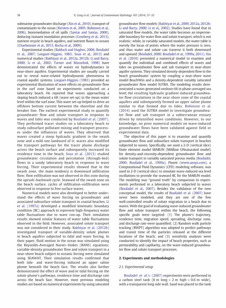
Fig. 1. Experimental laboratory beach setup showing conductivity meters(CMs), pressure transducers (PTs), water gauge (WG), and wave maker.
39X. Geng et al. / Journal of Contaminant Hydrology 165 (2014) 37–52
at a total horizontal length of 6.3 mat the base (Fig. 1). Thebeachslope was 10% between 0 m and 5 m distance, and a 40%between 5 m and 6.3 m distance (Fig. 1). The beach materialconsisted of coarse sand with a median size of 1 mm and aparticle size distribution varying from 0.8 mm to 1.2 mm.The porosity of the sand was 0.33. The saturated hydraulicconductivity was 2 × 10⁻³ m/s, and the values of vanGenuchten (1980) unsaturated parameters were α = 25 m−1
and n = 3.5. These parameterswere estimated by Boufadel et al.(1998) using a Bayesian approach. The open water level in thetank was measured using a wave gauge (WG, Model NO.LV5900, Omega Engineering). Four pressure transducers (PT,Model no. 1151AP, Fisher) were tapped into the side of the tankat 3 cm elevation from the tank bottom to measure waterpressure in the beach (Fig. 1). Ten conductivity meter sensors(CM, CDCN 108, Omega Engineering) were placed at differentlocations of the beach to measure salt concentrations (Fig. 1).The locations of all sensors are given in Table 1.
Two experiments with and without wave effects wereperformed in Boufadel et al. (2007). The tank was filledwith tap water which had a background ion concentration of0.15 g/L. The water level landward of the beach (PT1 in Fig. 1)was fixed at 1.0 m and the still water level (SWL) was fixed at0.9 m. The experiments were performed as follows: After asteady state hydraulic regime in the systemwas reached, 100 L
Table 1Location of pressure transducers, water gauge, and conductivity meters.
Note: x = horizontal distance from the screen (positive seaward); z =elevation from the bottom of the tank; y = horizontal depth from theplexiglass wall (positive inward perpendicular to the plan of Fig. 1). “NA”denotes that data are not applicable.
a The sensor is landward of the screen.
of NaCl solution at a concentration of 2.76 g/L was appliedonto the beach surface, at location of approximatelybetween x = 1.25 m and x = 1.50 m. The duration of thetracer application was about 50 min. For the wave experi-ments, the wavemaker was started immediately after thetracer application, and it was generating regular waves witha period of 1.11 s and height of 4.8 cm (see Boufadel et al.,2007 for details).
2.2. Methodologies of the numerical model
2.2.1. The MARUN modelNumerical simulations were conducted using the MARUN
(MARine UNsaturated) model, which can simulate density-dependent flow and solute transport in variably saturatedporous media (Boufadel, 2000; Boufadel et al., 1999a). Theequation for the conservation of water can be written as:
βϕ∂S∂t þ βS0S
∂ψ∂t þ ϕS
∂β∂t ¼
∂ βδKx∂ψ∂x
� �∂x þ
∂ βδKz∂ψ∂z
� �∂z
þ∂ β2δKz
� �∂z ; ð1Þ
where β is the density ratio [−] defined as ρ/ρ0 and δ is thedynamic viscosity ratio [−] defined as μ0/μ; ρ and ρ0 aresalt-dependent water density [ML−3] and freshwater density[ML−3], respectively; μ0 and μ are freshwater dynamicviscosity [ML−1 T−1] and salt-dependent water dynamicviscosity [ML−1 T−1]; ϕ is the porosity of the porous medium[−], S is the soil moisture ratio [−], S0 is the specific storage[L−1], ψ is the pressure head [L], and Kx and Kz are thehorizontal and vertical freshwater hydraulic conductivities[LT−1].
The soil moisture ratio S and freshwater hydraulicconductivities K are correlated by the van Genuchten (1980)model, which have the expressions as
For ψ≥0; S ¼ 1:0; Kx ¼ Kxo; Kz ¼ Kzo; ð2Þ
where Kxo and Kzo are the saturated horizontal and verticalfreshwater hydraulic conductivities, respectively.
For ψ b 0, the effective saturation ratio Se is given by:
Se ¼S−Sr1−Sr
¼ 11þ αjψjð Þn� �m
; ð3Þ
and Kx and Kz are given by
K j ¼ KjoSe1=2ð Þ 1− 1−Se
1=m� �mh i2
; ð4Þ
where j = (x, z), m = 1 − (1/n), Sr is the residual saturationratio, and |ψ| is the absolute value of ψ.
Following Boufadel et al. (1999a) and Boufadel (2000),the solute transport equation (convection–dispersion equa-tion) can be written as:
ϕS∂c∂t ¼ β∇ � ϕSD �∇cð Þ−q �∇c ð5Þ
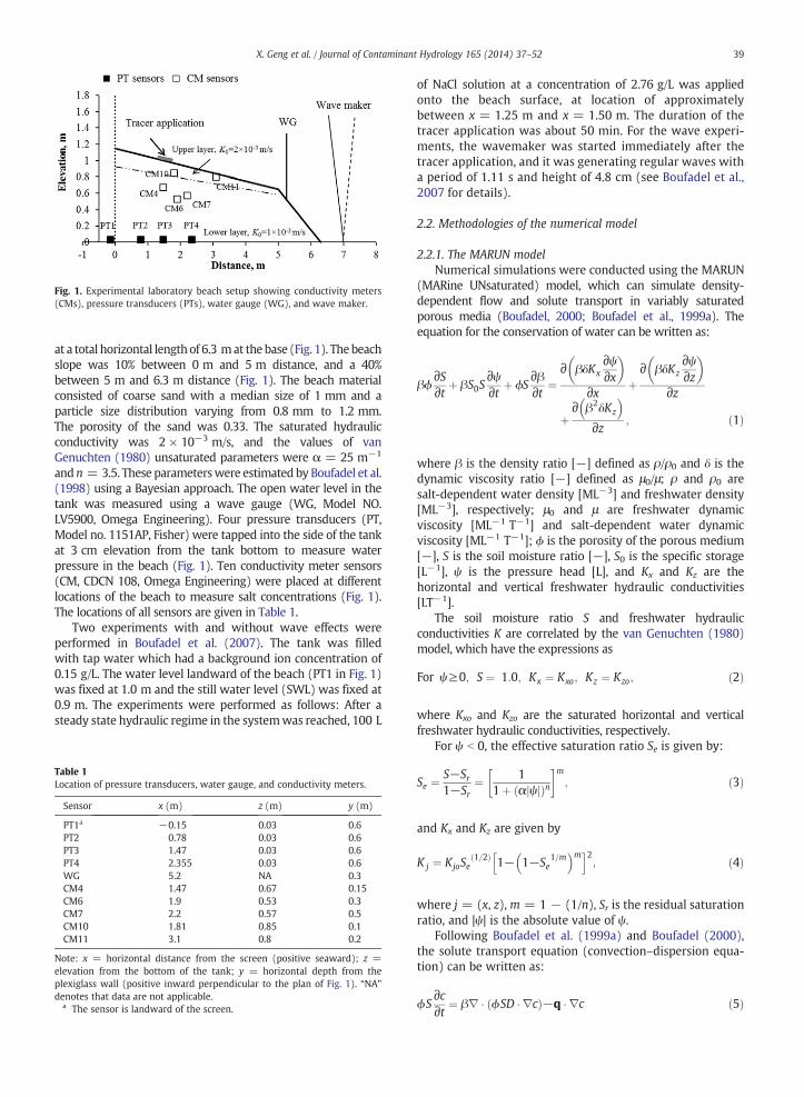
Fig. 2. Simulated wave run-up (a) and run-down (b) on the beach by usingFluent. Note that red color denotes water phase and blue color denotes airphase. The yellow color represents air pockets in the water.
40 X. Geng et al. / Journal of Contaminant Hydrology 165 (2014) 37–52
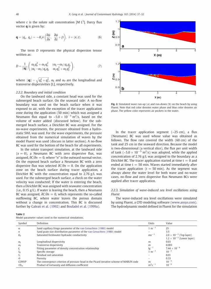
where c is the solute salt concentration [M L3]. Darcy fluxvector q is given by:
q ¼ qx; qzð Þ ¼ −Kiδ∂ψ∂x ;
∂ψ∂z þ β
� �; i ¼ x; zð Þ: ð6Þ
The term D represents the physical dispersion tensorwritten as:
D ¼ 1qj jj j
αLq2x þ αTq
2z αL−αTð Þqxqz
αL−αTð Þqxqz αTq2x þ αLq
2z
!; ð7Þ
where jjqjj ¼ffiffiffiffiffiffiffiffiffiffiffiffiffiffiffiffiq2x þ q2z
q, αL and αT are the longitudinal and
transverse dispersivities [L], respectively.
2.2.2. Boundary and initial conditionOn the landward side, a constant head was used for the
submerged beach surface. On the seaward side: A no-flowboundary was used on the beach surface when it wasexposed to air, with the exception of the tracer applicationzone during the application (50 min) which was assigned aNeumann flux equal to ~5.0 × 10⁻⁵ m2/s, based on thevolume of water added (discussed below). For the sub-merged beach surface, a Dirichlet BC was assigned. For theno-wave experiments, the pressure obtained from a hydro-static SWL was used. For the wave experiments, the pressureobtained from the numerical simulation of waves by themodel Fluent was used (discuss in latter section). A no-flowBC was used for the bottom of the beach for all experiments.
In the solute transport simulation, at the landward side(x = 0), a Neumann BC with zero dispersive flux, wasassigned, ∂C/∂n = 0, where “n” is the outward normal vector.On the exposed beach surface a Neumann BC with a zerodispersive flux was selected ∂C/∂n = 0. On the applicationzone on the beach surface during tracer application, aDirichlet BC with the concentration equal to 2.76 g/L wasused. For the submerged beach surface, a check on the watervelocity was conducted; If the water is entering the beach,then a Dirichlet BC was assigned with seawater concentration(i.e., 0.15 g/L). If water is leaving the beach, then a NeumannBC was assigned, ∂C/∂n = 0, which represents the so-calledoutflowing BC, where water leaves the porous domainwithout a change in concentration. This BC is discussedfurther by Galeati et al. (1992) and Boufadel et al. (1999a).
Table 2Model parameter values used in the numerical simulations.
Symbol Definition
α Sand capillary fringe parameter of the van Genuchten (1980) mon Sand grain size distribution parameter of the van Genuchten (198K0 Saturated freshwater hydraulic conductivity
αL Longitudinal dispersivityαT Transverse dispersivityξ Fitting parameter of density concentration relationshipS0 Specific storageSr Residual soil saturationΦ PorosityCONVP The convergence criterion of pressure head in the Picard iterativeτDm Product of tortuosity and diffusion coefficient
In the tracer application segment (~25 cm), a flux(Neumann) BC was used whose value was obtained asfollows. The flow rate covered the width (60 cm) of thetank and 25 cm in the seaward direction. Because the modelis two-dimensional (a vertical slice), the flux per unit widthof tank (~5.0 × 10⁻⁵ m2/s) was adopted, while the appliedconcentration of 2.76 g/L was assigned to the boundary as aDirichlet BC. The tracer application started at time t = 0 andended at time t = 50 min. Waves started immediately afterthe tracer application (t = 50 min). As the segment wasalways above the water level for both wave and no-wavecases, no-flow and zero dispersive flux Neumann BCs wereapplied after tracer application.
2.2.3. Simulation of wave-induced sea level oscillations usingFluent
The wave-induced sea level oscillations were simulatedby using Fluent, a CFD modeling software (www.ansys.com).The hydrodynamic model defined in Fluent for the simulation
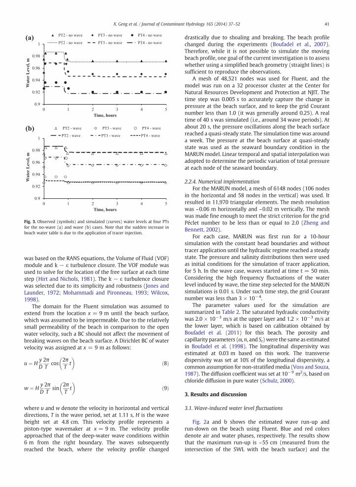
Fig. 3. Observed (symbols) and simulated (curves) water levels at four PTsfor the no-wave (a) and wave (b) cases. Note that the sudden increase inbeach water table is due to the application of tracer injection.
41X. Geng et al. / Journal of Contaminant Hydrology 165 (2014) 37–52
was based on the RANS equations, the Volume of Fluid (VOF)module and k − ε turbulence closure. The VOF module wasused to solve for the location of the free surface at each timestep (Hirt and Nichols, 1981). The k − ε turbulence closurewas selected due to its simplicity and robustness (Jones andLaunder, 1972; Mohammadi and Pironneau, 1993; Wilcox,1998).
The domain for the Fluent simulation was assumed toextend from the location x = 9 m until the beach surface,which was assumed to be impermeable. Due to the relativelysmall permeability of the beach in comparison to the openwater velocity, such a BC should not affect the movement ofbreaking waves on the beach surface. A Dirichlet BC of watervelocity was assigned at x = 9 m as follows:
u ¼ HyD2πT
cos2πT
t� �
ð8Þ
w ¼ HyD2πT
sin2πT
t� �
ð9Þ
where u and w denote the velocity in horizontal and verticaldirections, T is the wave period, set at 1.11 s, H is the waveheight set at 4.8 cm. This velocity profile represents apiston-type wavemaker at x = 9 m. The velocity profileapproached that of the deep-water wave conditions within6 m from the right boundary. The waves subsequentlyreached the beach, where the velocity profile changed
drastically due to shoaling and breaking. The beach profilechanged during the experiments (Boufadel et al., 2007).Therefore, while it is not possible to simulate the movingbeach profile, one goal of the current investigation is to assesswhether using a simplified beach geometry (straight lines) issufficient to reproduce the observations.
A mesh of 48,521 nodes was used for Fluent, and themodel was run on a 32 processor cluster at the Center forNatural Resources Development and Protection at NJIT. Thetime step was 0.005 s to accurately capture the change inpressure at the beach surface, and to keep the grid Courantnumber less than 1.0 (it was generally around 0.25). A realtime of 40 s was simulated (i.e., around 34 wave periods). Atabout 20 s, the pressure oscillations along the beach surfacereached a quasi-steady state. The simulation timewas arounda week. The pressure at the beach surface at quasi-steadystate was used as the seaward boundary condition in theMARUNmodel. Linear temporal and spatial interpolation wasadopted to determine the periodic variation of total pressureat each node of the seaward boundary.
2.2.4. Numerical implementationFor the MARUN model, a mesh of 6148 nodes (106 nodes
in the horizontal and 58 nodes in the vertical) was used. Itresulted in 11,970 triangular elements. The mesh resolutionwas ~0.06 m horizontally and ~0.02 m vertically. The meshwas made fine enough to meet the strict criterion for the gridPéclet number to be less than or equal to 2.0 (Zheng andBennett, 2002).
For each case, MARUN was first run for a 10-hoursimulation with the constant head boundaries and withouttracer application until the hydraulic regime reached a steadystate. The pressure and salinity distributions then were usedas initial conditions for the simulation of tracer application,for 5 h. In the wave case, waves started at time t = 50 min.Considering the high frequency fluctuations of the waterlevel induced by wave, the time step selected for the MARUNsimulations is 0.01 s. Under such time step, the grid Courantnumber was less than 3 × 10⁻⁴.
The parameter values used for the simulation aresummarized in Table 2. The saturated hydraulic conductivitywas 2.0 × 10⁻³ m/s at the upper layer and 1.2 × 10⁻³ m/s atthe lower layer, which is based on calibration obtained byBoufadel et al. (2011) for this beach. The porosity andcapillarity parameters (α, n, and Sr)were the same as estimatedin Boufadel et al. (1998). The longitudinal dispersivity wasestimated at 0.03 m based on this work. The transversedispersivity was set at 10% of the longitudinal dispersivity, acommon assumption for non-stratifiedmedia (Voss and Souza,1987). The diffusion coefficient was set at 10−9 m2/s, based onchloride diffusion in pure water (Schulz, 2000).
3. Results and discussion
3.1. Wave-induced water level fluctuations
Fig. 2a and b shows the estimated wave run-up andrun-down on the beach using Fluent. Blue and red colorsdenote air and water phases, respectively. The results showthat the maximum run-up is ~55 cm (measured from theintersection of the SWL with the beach surface) and the
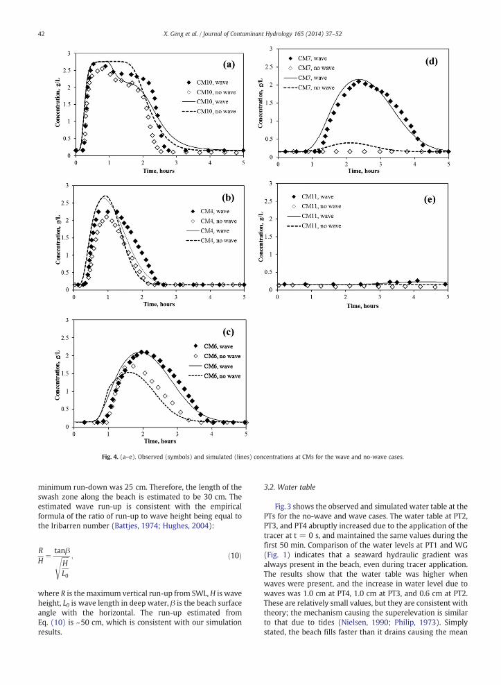
Fig. 4. (a–e). Observed (symbols) and simulated (lines) concentrations at CMs for the wave and no-wave cases.
42 X. Geng et al. / Journal of Contaminant Hydrology 165 (2014) 37–52
minimum run-down was 25 cm. Therefore, the length of theswash zone along the beach is estimated to be 30 cm. Theestimated wave run-up is consistent with the empiricalformula of the ratio of run-up to wave height being equal tothe Iribarren number (Battjes, 1974; Hughes, 2004):
RH
¼ tanβffiffiffiffiffiHL0
s ; ð10Þ
where R is the maximum vertical run-up from SWL, H is waveheight, L0 is wave length in deep water, β is the beach surfaceangle with the horizontal. The run-up estimated fromEq. (10) is ~50 cm, which is consistent with our simulationresults.
3.2. Water table
Fig. 3 shows the observed and simulated water table at thePTs for the no-wave and wave cases. The water table at PT2,PT3, and PT4 abruptly increased due to the application of thetracer at t = 0 s, and maintained the same values during thefirst 50 min. Comparison of the water levels at PT1 and WG(Fig. 1) indicates that a seaward hydraulic gradient wasalways present in the beach, even during tracer application.The results show that the water table was higher whenwaves were present, and the increase in water level due towaves was 1.0 cm at PT4, 1.0 cm at PT3, and 0.6 cm at PT2.These are relatively small values, but they are consistent withtheory; the mechanism causing the superelevation is similarto that due to tides (Nielsen, 1990; Philip, 1973). Simplystated, the beach fills faster than it drains causing the mean
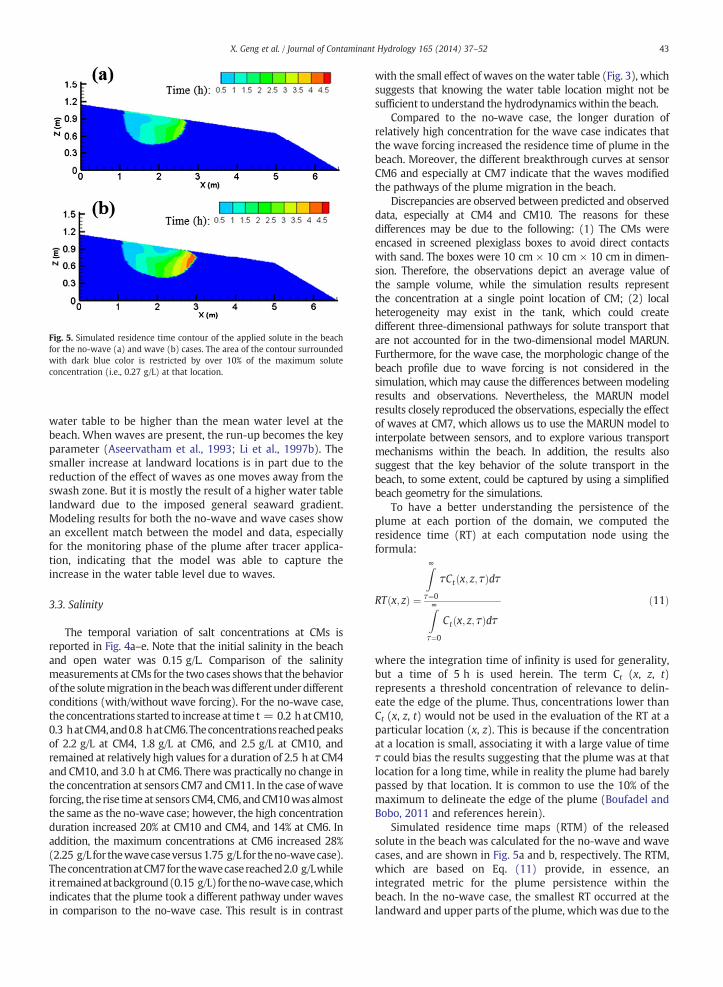
Fig. 5. Simulated residence time contour of the applied solute in the beachfor the no-wave (a) and wave (b) cases. The area of the contour surroundedwith dark blue color is restricted by over 10% of the maximum soluteconcentration (i.e., 0.27 g/L) at that location.
43X. Geng et al. / Journal of Contaminant Hydrology 165 (2014) 37–52
water table to be higher than the mean water level at thebeach. When waves are present, the run-up becomes the keyparameter (Aseervatham et al., 1993; Li et al., 1997b). Thesmaller increase at landward locations is in part due to thereduction of the effect of waves as one moves away from theswash zone. But it is mostly the result of a higher water tablelandward due to the imposed general seaward gradient.Modeling results for both the no-wave and wave cases showan excellent match between the model and data, especiallyfor the monitoring phase of the plume after tracer applica-tion, indicating that the model was able to capture theincrease in the water table level due to waves.
3.3. Salinity
The temporal variation of salt concentrations at CMs isreported in Fig. 4a–e. Note that the initial salinity in the beachand open water was 0.15 g/L. Comparison of the salinitymeasurements at CMs for the two cases shows that the behaviorof the solutemigration in thebeachwasdifferentunderdifferentconditions (with/without wave forcing). For the no-wave case,theconcentrations started to increase at time t = 0.2 hatCM10,0.3 hatCM4,and0.8 hatCM6.Theconcentrationsreachedpeaksof 2.2 g/L at CM4, 1.8 g/L at CM6, and 2.5 g/L at CM10, andremained at relatively high values for a duration of 2.5 h at CM4and CM10, and 3.0 h at CM6. There was practically no change inthe concentration at sensors CM7 and CM11. In the case ofwaveforcing, the rise timeat sensorsCM4, CM6, andCM10wasalmostthe same as the no-wave case; however, the high concentrationduration increased 20% at CM10 and CM4, and 14% at CM6. Inaddition, the maximum concentrations at CM6 increased 28%(2.25 g/L for thewavecaseversus1.75 g/L for theno-wavecase).TheconcentrationatCM7forthewavecasereached2.0 g/Lwhileitremainedatbackground(0.15 g/L)fortheno-wavecase,whichindicates that the plume took a different pathway under wavesin comparison to the no-wave case. This result is in contrast
with the small effect of waves on the water table (Fig. 3), whichsuggests that knowing the water table location might not besufficient to understand the hydrodynamicswithin the beach.
Compared to the no-wave case, the longer duration ofrelatively high concentration for the wave case indicates thatthe wave forcing increased the residence time of plume in thebeach. Moreover, the different breakthrough curves at sensorCM6 and especially at CM7 indicate that the waves modifiedthe pathways of the plume migration in the beach.
Discrepancies are observed between predicted and observeddata, especially at CM4 and CM10. The reasons for thesedifferences may be due to the following: (1) The CMs wereencased in screened plexiglass boxes to avoid direct contactswith sand. The boxes were 10 cm × 10 cm × 10 cm in dimen-sion. Therefore, the observations depict an average value ofthe sample volume, while the simulation results representthe concentration at a single point location of CM; (2) localheterogeneity may exist in the tank, which could createdifferent three-dimensional pathways for solute transport thatare not accounted for in the two-dimensional model MARUN.Furthermore, for the wave case, the morphologic change of thebeach profile due to wave forcing is not considered in thesimulation, which may cause the differences between modelingresults and observations. Nevertheless, the MARUN modelresults closely reproduced the observations, especially the effectof waves at CM7, which allows us to use the MARUN model tointerpolate between sensors, and to explore various transportmechanisms within the beach. In addition, the results alsosuggest that the key behavior of the solute transport in thebeach, to some extent, could be captured by using a simplifiedbeach geometry for the simulations.
To have a better understanding the persistence of theplume at each portion of the domain, we computed theresidence time (RT) at each computation node using theformula:
RT x; zð Þ ¼
Z∞τ¼0
τCt x; z; τð Þdτ
Z∞τ¼0
Ct x; z; τð Þdτð11Þ
where the integration time of infinity is used for generality,but a time of 5 h is used herein. The term Ct (x, z, t)represents a threshold concentration of relevance to delin-eate the edge of the plume. Thus, concentrations lower thanCt (x, z, t) would not be used in the evaluation of the RT at aparticular location (x, z). This is because if the concentrationat a location is small, associating it with a large value of timeτ could bias the results suggesting that the plume was at thatlocation for a long time, while in reality the plume had barelypassed by that location. It is common to use the 10% of themaximum to delineate the edge of the plume (Boufadel andBobo, 2011 and references herein).
Simulated residence time maps (RTM) of the releasedsolute in the beach was calculated for the no-wave and wavecases, and are shown in Fig. 5a and b, respectively. The RTM,which are based on Eq. (11) provide, in essence, anintegrated metric for the plume persistence within thebeach. In the no-wave case, the smallest RT occurred at thelandward and upper parts of the plume, which was due to the
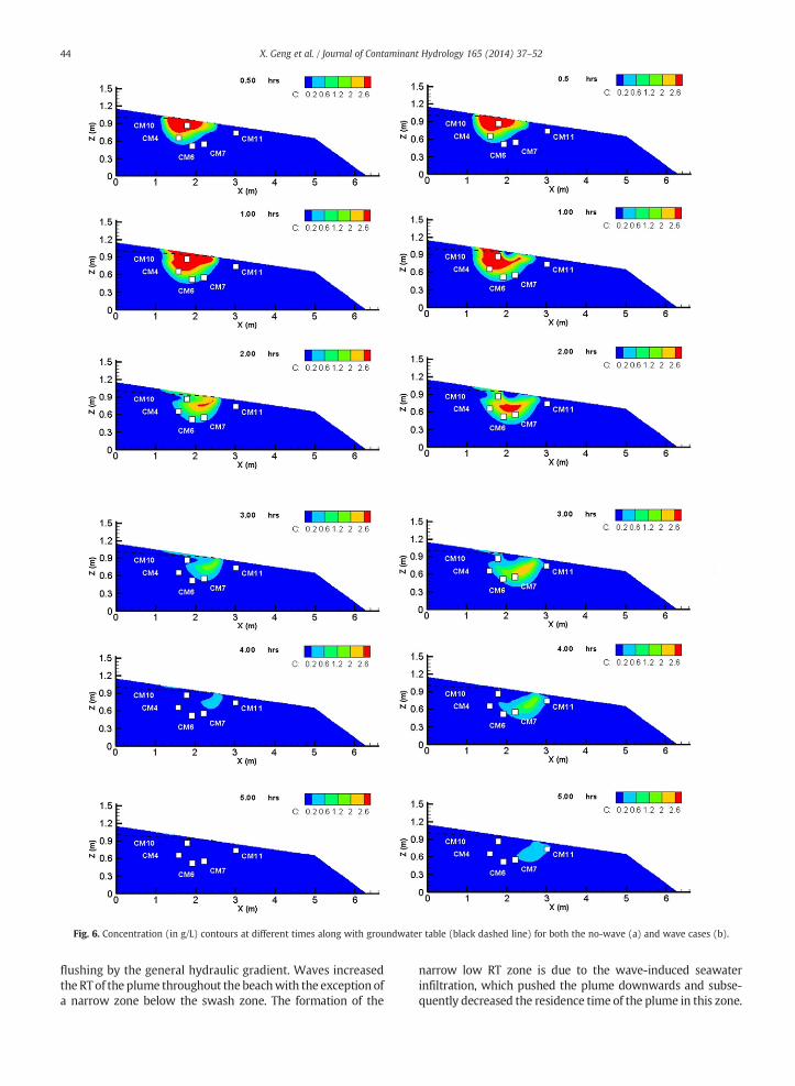
Fig. 6. Concentration (in g/L) contours at different times along with groundwater table (black dashed line) for both the no-wave (a) and wave cases (b).
44 X. Geng et al. / Journal of Contaminant Hydrology 165 (2014) 37–52
flushing by the general hydraulic gradient. Waves increasedthe RTof the plume throughout the beachwith the exception ofa narrow zone below the swash zone. The formation of the
narrow low RT zone is due to the wave-induced seawaterinfiltration, which pushed the plume downwards and subse-quently decreased the residence time of the plume in this zone.
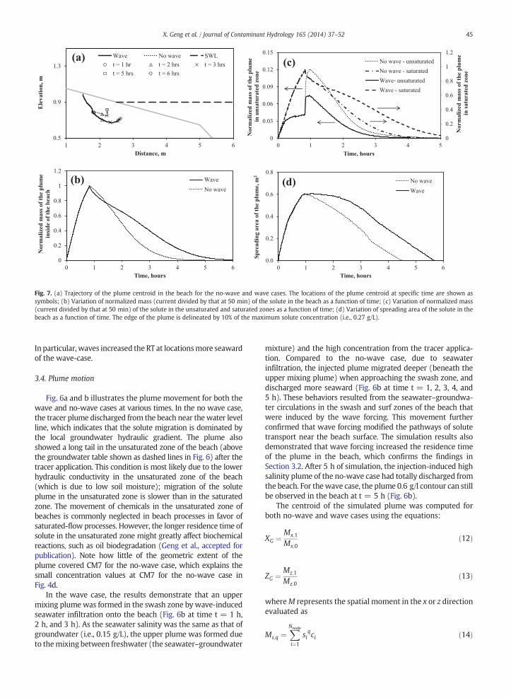
Fig. 7. (a) Trajectory of the plume centroid in the beach for the no-wave and wave cases. The locations of the plume centroid at specific time are shown assymbols; (b) Variation of normalized mass (current divided by that at 50 min) of the solute in the beach as a function of time; (c) Variation of normalized mass(current divided by that at 50 min) of the solute in the unsaturated and saturated zones as a function of time; (d) Variation of spreading area of the solute in thebeach as a function of time. The edge of the plume is delineated by 10% of the maximum solute concentration (i.e., 0.27 g/L).
45X. Geng et al. / Journal of Contaminant Hydrology 165 (2014) 37–52
In particular, waves increased the RT at locationsmore seawardof the wave-case.
3.4. Plume motion
Fig. 6a and b illustrates the plume movement for both thewave and no-wave cases at various times. In the no wave case,the tracer plume discharged from the beach near the water levelline, which indicates that the solute migration is dominated bythe local groundwater hydraulic gradient. The plume alsoshowed a long tail in the unsaturated zone of the beach (abovethe groundwater table shown as dashed lines in Fig. 6) after thetracer application. This condition is most likely due to the lowerhydraulic conductivity in the unsaturated zone of the beach(which is due to low soil moisture); migration of the soluteplume in the unsaturated zone is slower than in the saturatedzone. The movement of chemicals in the unsaturated zone ofbeaches is commonly neglected in beach processes in favor ofsaturated-flow processes. However, the longer residence time ofsolute in the unsaturated zone might greatly affect biochemicalreactions, such as oil biodegradation (Geng et al., accepted forpublication). Note how little of the geometric extent of theplume covered CM7 for the no-wave case, which explains thesmall concentration values at CM7 for the no-wave case inFig. 4d.
In the wave case, the results demonstrate that an uppermixing plumewas formed in the swash zone by wave-inducedseawater infiltration onto the beach (Fig. 6b at time t = 1 h,2 h, and 3 h). As the seawater salinity was the same as that ofgroundwater (i.e., 0.15 g/L), the upper plume was formed dueto themixing between freshwater (the seawater–groundwater
mixture) and the high concentration from the tracer applica-tion. Compared to the no-wave case, due to seawaterinfiltration, the injected plume migrated deeper (beneath theupper mixing plume) when approaching the swash zone, anddischarged more seaward (Fig. 6b at time t = 1, 2, 3, 4, and5 h). These behaviors resulted from the seawater–groundwa-ter circulations in the swash and surf zones of the beach thatwere induced by the wave forcing. This movement furtherconfirmed that wave forcing modified the pathways of solutetransport near the beach surface. The simulation results alsodemonstrated that wave forcing increased the residence timeof the plume in the beach, which confirms the findings inSection 3.2. After 5 h of simulation, the injection-induced highsalinity plume of the no-wave case had totally discharged fromthe beach. For thewave case, the plume 0.6 g/l contour can stillbe observed in the beach at t = 5 h (Fig. 6b).
The centroid of the simulated plume was computed forboth no-wave and wave cases using the equations:
XG ¼ Mx;1
Mx;0ð12Þ
ZG ¼ Mz;1
Mz;0ð13Þ
whereM represents the spatial moment in the x or z directionevaluated as
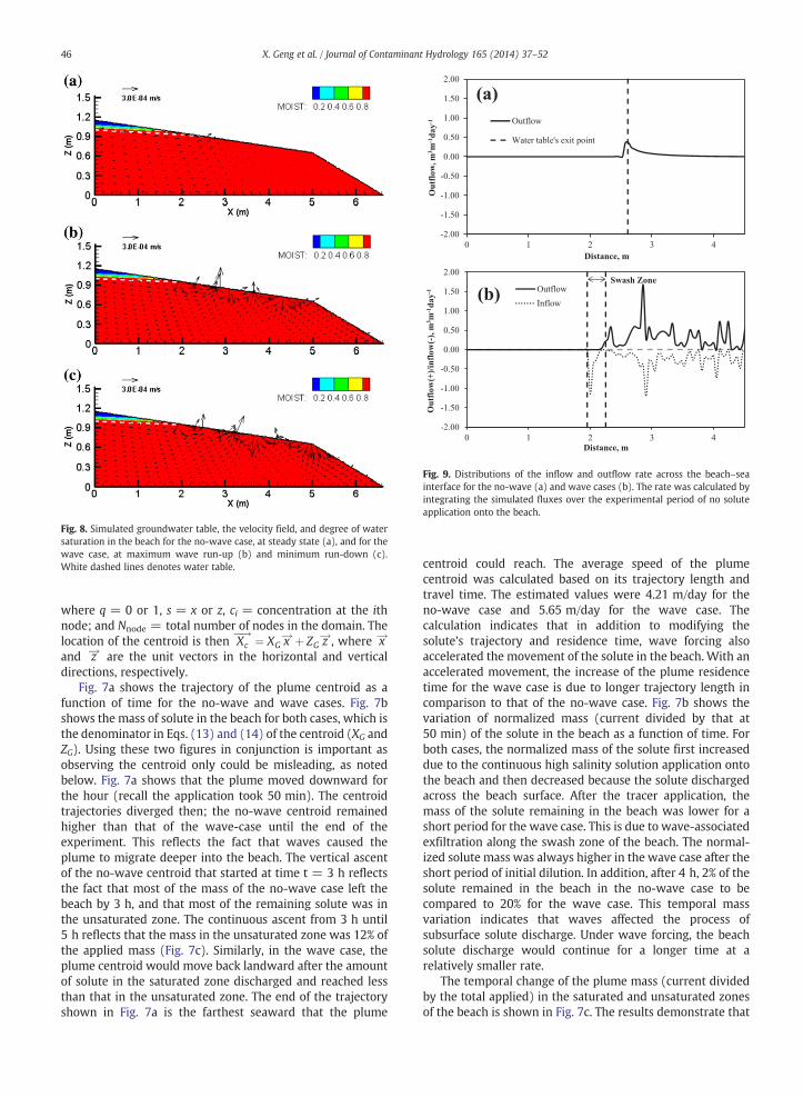
Fig. 8. Simulated groundwater table, the velocity field, and degree of watersaturation in the beach for the no-wave case, at steady state (a), and for thewave case, at maximum wave run-up (b) and minimum run-down (c).White dashed lines denotes water table.
-2.00
-1.50
-1.00
-0.50
0.00
0.50
1.00
1.50
2.00
0 1 2 3 4
Out
flow
, m3 m
-1da
y-1
Distance, m
Outflow
Water table's exit point
(a)
-2.00
-1.50
-1.00
-0.50
0.00
0.50
1.00
1.50
2.00
0 1 2 3 4O
utflo
w(+
)/inf
low
(-),
m3 m
-1da
y- 1
Distance, m
Outflow
Inflow(b)
Swash Zone
Fig. 9. Distributions of the inflow and outflow rate across the beach–seainterface for the no-wave (a) and wave cases (b). The rate was calculated byintegrating the simulated fluxes over the experimental period of no soluteapplication onto the beach.
46 X. Geng et al. / Journal of Contaminant Hydrology 165 (2014) 37–52
where q = 0 or 1, s = x or z, ci = concentration at the ithnode; and Nnode = total number of nodes in the domain. Thelocation of the centroid is then Xc
! ¼ XG x!þ ZG z!, where x!and z! are the unit vectors in the horizontal and verticaldirections, respectively.
Fig. 7a shows the trajectory of the plume centroid as afunction of time for the no-wave and wave cases. Fig. 7bshows the mass of solute in the beach for both cases, which isthe denominator in Eqs. (13) and (14) of the centroid (XG andZG). Using these two figures in conjunction is important asobserving the centroid only could be misleading, as notedbelow. Fig. 7a shows that the plume moved downward forthe hour (recall the application took 50 min). The centroidtrajectories diverged then; the no-wave centroid remainedhigher than that of the wave-case until the end of theexperiment. This reflects the fact that waves caused theplume to migrate deeper into the beach. The vertical ascentof the no-wave centroid that started at time t = 3 h reflectsthe fact that most of the mass of the no-wave case left thebeach by 3 h, and that most of the remaining solute was inthe unsaturated zone. The continuous ascent from 3 h until5 h reflects that the mass in the unsaturated zone was 12% ofthe applied mass (Fig. 7c). Similarly, in the wave case, theplume centroid would move back landward after the amountof solute in the saturated zone discharged and reached lessthan that in the unsaturated zone. The end of the trajectoryshown in Fig. 7a is the farthest seaward that the plume
centroid could reach. The average speed of the plumecentroid was calculated based on its trajectory length andtravel time. The estimated values were 4.21 m/day for theno-wave case and 5.65 m/day for the wave case. Thecalculation indicates that in addition to modifying thesolute's trajectory and residence time, wave forcing alsoaccelerated the movement of the solute in the beach. With anaccelerated movement, the increase of the plume residencetime for the wave case is due to longer trajectory length incomparison to that of the no-wave case. Fig. 7b shows thevariation of normalized mass (current divided by that at50 min) of the solute in the beach as a function of time. Forboth cases, the normalized mass of the solute first increaseddue to the continuous high salinity solution application ontothe beach and then decreased because the solute dischargedacross the beach surface. After the tracer application, themass of the solute remaining in the beach was lower for ashort period for the wave case. This is due to wave-associatedexfiltration along the swash zone of the beach. The normal-ized solute mass was always higher in the wave case after theshort period of initial dilution. In addition, after 4 h, 2% of thesolute remained in the beach in the no-wave case to becompared to 20% for the wave case. This temporal massvariation indicates that waves affected the process ofsubsurface solute discharge. Under wave forcing, the beachsolute discharge would continue for a longer time at arelatively smaller rate.
The temporal change of the plume mass (current dividedby the total applied) in the saturated and unsaturated zonesof the beach is shown in Fig. 7c. The results demonstrate that
47X. Geng et al. / Journal of Contaminant Hydrology 165 (2014) 37–52
waves significantly decreased the solute discharge rate insaturated zone of the beach. After 3 h, only 10% of the plumemass remained in the beach for the no-wave case, while 40%of the plume mass still remained in the beach subjected towaves. The results also suggest that in addition to affectingsolute transport in the saturated zone, wave forcing alsoaffects solute transport behavior in the unsaturated zone ofthe beach. In the absence of wave forcing, the normalizedmass in the unsaturated zone first increased gradually to 4%until the end of application (t = 50 min), and then it roseabruptly reaching its peak of 13% within 10 min. The gradualincrease of the solute mass in the unsaturated zone alongwith the rise in the water table is due to the continuouspercolation of applied solution into the beach. After theapplication, the water table elevation rapidly decreased to itsinitial condition (shown in Fig. 3). This sudden decreasecaused a certain amount of solute to remain above the watertable in the beach, which increased the proportion of solutemass in the unsaturated zone. Therefore, the normalizedmass curve shows an abrupt rise within a short period afterthe tracer application. Under wave forcing, the change of thesolute mass in the unsaturated zone reveals a similar trendbut the proportion of solute mass in the unsaturated zone ismuch smaller. The reasons for these differences are asfollows: The wave-induced seawater infiltration in swashzone of the beach drove more solute downwards to thesaturated zone of the beach, and subsequently decreased theproportion of the mass in the unsaturated zone. In addition,the infiltration in the swash zone due to waves narrowed theunsaturated zone of the beach and subsequently reduced thesolute mass in the unsaturated zone. Fig. 7d show the
0
0.2
0.4
0.6
0.8
1
1.2
1.4
0 1 2 3 4
Ele
vatio
n, m
Distance, m
No wave Wave
SWL
(a)
0 10 20 30 40 50
0.1
0.3
0.5
0.7
0.9
Time, hour
Ele
vatio
n, m
No wave Wave (b)
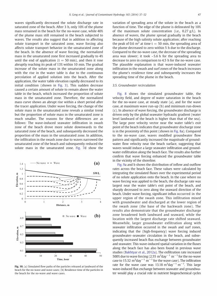
Fig. 10. (a) Simulated flow paths of the particles released at landward of thebeach for the no-wave and wave cases; (b) Residence time of the particles inthe beach for the no-wave and wave cases.
variation of spreading area of the solute in the beach as afunction of time. The edge of the plume is delineated by 10%of the maximum solute concentration (i.e., 0.27 g/L). Inabsence of waves, the plume spread gradually in the beachbecause of the high salinity solute application; after reachingthe peak of 0.6 m2 at time t = 50 min, the spreading area ofthe plume decreased to zero within 5 h due to the discharge.Compared to the no-wave case, the decrease of the spreadingarea was slower; it took ~5.6 h for the spreading area todecrease to zero in comparison to 4.5 h for the no-wave case.The plausible explanation is that wave-induced seawaterinfiltration in the swash and surf zones of the beach increasesthe plume's residence time and subsequently increases thespreading time of the plume in the beach.
3.5. Groundwater recirculation
Fig. 8 shows the simulated groundwater table, thevelocity field, and degree of water saturation in the beachfor the no-wave case, at steady state (a), and for the wavecase, at maximum wave run-up (b) and minimum run-down(c). In absence of wave forcing, the groundwater discharge isdriven only by the global seawater hydraulic gradient (waterlevel landward of the beach is higher than that of the sea).The large pore velocity vector near the water table's exitpoint of the beach indicates that groundwater discharge zoneis in the proximity of this point (shown in Fig. 8a). Comparedto the no-wave case, waves modified groundwater flowpattern and significantly increased the magnitude of ground-water flow velocity near the beach surface, suggesting thatwaves would induce a large seawater infiltration and ground-water exfiltration along the beach face. The results also furtherconfirm that wave forcing enhanced the groundwater tablein the vicinity of the shoreline.
Fig. 9a and b shows the distribution of inflow and outflowrates across the beach face. These values were calculated byintegrating the simulated fluxes over the experimental periodof no solute application onto the beach. In the case where nowave forcing was applied to the beach, the discharge rate waslargest near the water table's exit point of the beach, andsharply decreased to zero along the seaward direction of thebeach. Under wave forcing, significant influx occurred in theupper region of the swash zone. This infiltration mixedwith groundwater and discharged at the lower region ofthe swash zone (the base of the backwash zone). Theresults also demonstrate that the groundwater dischargezone broadened both landward and seaward, while thelocation with the largest discharge rate shifted seaward.Meanwhile, larger groundwater exfiltration along withseawater infiltration occurred in the swash and surf zones,indicating that the (high-frequency) wave forcing inducedgroundwater–seawater circulation in the beach, and subse-quently increased beach flux exchange between groundwaterand seawater. This wave-induced spatial variation in the fluxesalong the beach face has also been found in previous wavestudies (Bakhtyar et al., 2012a). The exfiltration rate increased500% due towave forcing (2.55 m3day−1 m−1 for the no-wavecase to 15.32 m3day−1 m−1 for the wave case). The infiltrationrate for the wave case was 13.18 m3day−1 m−1. This largewave-induced flux exchange between seawater and groundwa-ter would play a crucial role in nutrient biogeochemical cycles
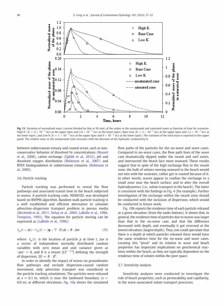
Fig. 11. Variation of normalized mass (current divided by that at 50 min) of the solute in the unsaturated and saturated zones as function of time for scenarios.High K: (K = 4 × 10⁻³ m/s at the upper layer and 2.4 × 10⁻³ m/s at the lower layer), Base Case (K = 2 × 10⁻³ m/s at the upper layer and 1.2 × 10⁻³ m/s atthe lower layer), and Low K (K = 1 × 10⁻³ m/s at the upper layer and 6 × 10⁻⁴ m/s at the lower layer). The variation of the total mass is reported in the upperpanel. The relative mass in the unsaturated zone increases with the decrease of the hydraulic conductivity K.
48 X. Geng et al. / Journal of Contaminant Hydrology 165 (2014) 37–52
between subterranean estuary and coastal ocean, such as non-conservative behavior of dissolved Fe concentrations (Rouxelet al., 2008), cation exchange (Zghibi et al., 2012), pH anddissolved oxygen distribution (Robinson et al., 2007) andBTEX biodegradation in subterranean estuaries (Robinson etal., 2009).
3.6. Particle tracking
Particle tracking was performed to reveal the flowpathways and associated transit time in the beach subjectedto waves. A particle tracking code, NEMO3D, was developedbased on RWPM algorithm. Random walk particle tracking isa well established and efficient alternative to simulateadvection–dispersion transport problem in porous media(Bechtold et al., 2011; Delay et al., 2005; LaBolle et al., 1996;Tompson, 1993). The equation for particle moving can beexpressed as (LaBolle et al., 1996):
X!p t þ Δtð Þ−X
!p tð Þ ¼ qþ∇ � Dð ÞΔt þ B � Δw ð15Þ
where X!p tð Þ is the location of particle p at time t, Δw is
a vector of independent normally distributed randomvariables with zero mean and unit variance given as⟨Δw⟩ = 0, and B is a tensor [LT−1/2] defining the strengthof dispersion, 2D = B ⋅ BT.
In order to identify the impact of waves on groundwaterflow pathways and exclude dispersion-caused randommovement, only advection transport was considered inthe particle tracking simulations. The particles were releasedat x = 0.1 m, which is near the landward boundary (x =0.0 m) at different elevations. Fig. 10a shows the simulated
flow paths of the particles for the no-wave and wave cases.Compared to no-wave cases, the flow path lines of the wavecase dramatically dipped under the swash and surf zones,and intersected the beach face more seaward. These resultssuggest that in spite of the high exchange flux in the swashzone, the bulk of solutes moving seaward in the beach wouldnot mix with the seawater, rather get re-routed because of it.In other words, waves appear to confine the exchange to asmall zone near the beach surface, and to alter the overallhydrodynamics (i.e., solute transport in the beach). The latteris consistent with the findings in Fig. 4 (for example). Furtherinvestigation of the exchange within the swash zone shouldbe conducted with the inclusion of dispersion, which wouldbe conducted in future work.
Fig. 10b reports the residence time of each particle releasedat a given elevation (from the tanks bottom). It shows that, ingeneral, the residence time of particles due towaveswas largerthan that in the no-wave case, and that the differencedecreased with depth, and eventually it got reversed at thelowest elevation (largest depth). Thus, one could speculate thatthere is a depth at which particles released there would havethe same residence time for the no-wave and wave cases.Locating this “pivot” and its relation to wave and beachproperties has important implications on geochemical reac-tions within the beach, as they are typically dependent on theresidence time of solutes within the pore space.
3.7. Sensitivity analysis
Sensitivity analyses were conducted to investigate therole of beach properties, such as permeability and capillarity,in the wave-associated solute transport processes.
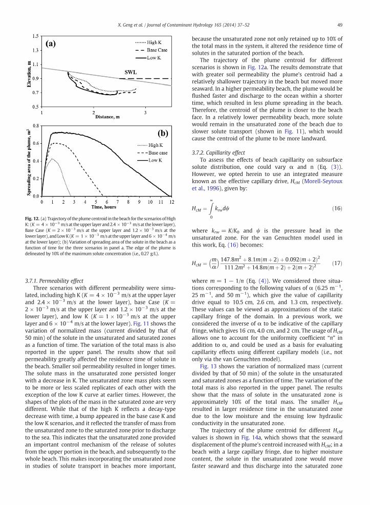
Fig. 12. (a) Trajectory of theplumecentroid in thebeach for the scenariosofHighK: (K = 4 × 10⁻³ m/s at theupper layer and2.4 × 10−3 m/s at the lower layer),Base Case (K = 2 × 10⁻³ m/s at the upper layer and 1.2 × 10⁻³ m/s at thelower layer), andLowK(K = 1 × 10⁻³ m/sat theupper layer and6 × 10−4 m/sat the lower layer); (b) Variation of spreading area of the solute in the beach as afunction of time for the three scenarios in panel a. The edge of the plume isdelineated by 10% of the maximum solute concentration (i.e., 0.27 g/L).
49X. Geng et al. / Journal of Contaminant Hydrology 165 (2014) 37–52
3.7.1. Permeability effectThree scenarios with different permeability were simu-
lated, including high K (K = 4 × 10⁻³ m/s at the upper layerand 2.4 × 10⁻³ m/s at the lower layer), base Case (K =2 × 10⁻³ m/s at the upper layer and 1.2 × 10⁻³ m/s at thelower layer), and low K (K = 1 × 10⁻³ m/s at the upperlayer and 6 × 10⁻⁴ m/s at the lower layer). Fig. 11 shows thevariation of normalized mass (current divided by that of50 min) of the solute in the unsaturated and saturated zonesas a function of time. The variation of the total mass is alsoreported in the upper panel. The results show that soilpermeability greatly affected the residence time of solute inthe beach. Smaller soil permeability resulted in longer times.The solute mass in the unsaturated zone persisted longerwith a decrease in K. The unsaturated zone mass plots seemto be more or less scaled replicates of each other with theexception of the low K curve at earlier times. However, theshapes of the plots of the mass in the saturated zone are verydifferent. While that of the high K reflects a decay-typedecrease with time, a bump appeared in the base case K andthe low K scenarios, and it reflected the transfer of mass fromthe unsaturated zone to the saturated zone prior to dischargeto the sea. This indicates that the unsaturated zone providedan important control mechanism of the release of solutesfrom the upper portion in the beach, and subsequently to thewhole beach. This makes incorporating the unsaturated zonein studies of solute transport in beaches more important,
because the unsaturated zone not only retained up to 10% ofthe total mass in the system, it altered the residence time ofsolutes in the saturated portion of the beach.
The trajectory of the plume centroid for differentscenarios is shown in Fig. 12a. The results demonstrate thatwith greater soil permeability the plume's centroid had arelatively shallower trajectory in the beach but moved moreseaward. In a higher permeability beach, the plume would beflushed faster and discharge to the ocean within a shortertime, which resulted in less plume spreading in the beach.Therefore, the centroid of the plume is closer to the beachface. In a relatively lower permeability beach, more solutewould remain in the unsaturated zone of the beach due toslower solute transport (shown in Fig. 11), which wouldcause the centroid of the plume to be more landward.
3.7.2. Capillarity effectTo assess the effects of beach capillarity on subsurface
solute distribution, one could vary α and n (Eq. (3)).However, we opted herein to use an integrated measureknown as the effective capillary drive, HcM (Morell-Seytouxet al., 1996), given by:
HcM ¼Z∞0
krwdψ ð16Þ
where krw = K/K0 and ψ is the pressure head in theunsaturated zone. For the van Genuchten model used inthis work, Eq. (16) becomes:
where m = 1 − 1/n (Eq. (4)). We considered three situa-tions corresponding to the following values of α (6.25 m−1,25 m−1, and 50 m−1), which give the value of capillaritydrive equal to 10.5 cm, 2.6 cm, and 1.3 cm, respectively.These values can be viewed as approximations of the staticcapillary fringe of the domain. In a previous work, weconsidered the inverse of α to be indicative of the capillaryfringe, which gives 16 cm, 4.0 cm, and 2 cm. The usage of HcM
allows one to account for the uniformity coefficient “n” inaddition to α, and could be used as a basis for evaluatingcapillarity effects using different capillary models (i.e., notonly via the van Genuchten model).
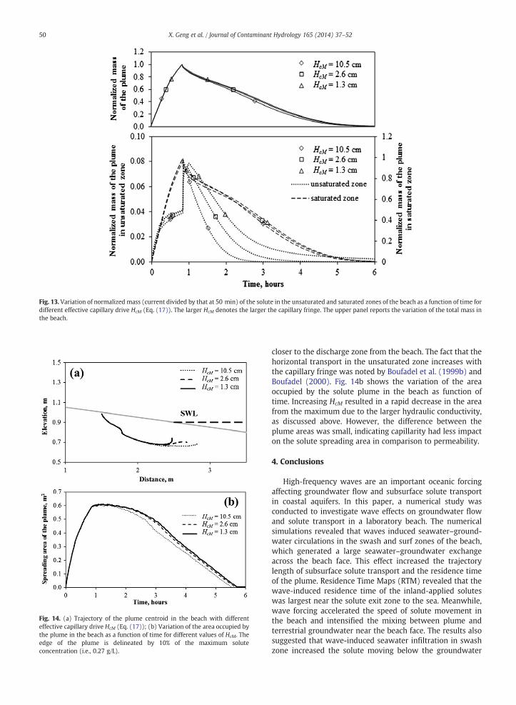
Fig. 13 shows the variation of normalized mass (currentdivided by that of 50 min) of the solute in the unsaturatedand saturated zones as a function of time. The variation of thetotal mass is also reported in the upper panel. The resultsshow that the mass of solute in the unsaturated zone isapproximately 10% of the total mass. The smaller HcM
resulted in larger residence time in the unsaturated zonedue to the low moisture and the ensuing low hydraulicconductivity in the unsaturated zone.
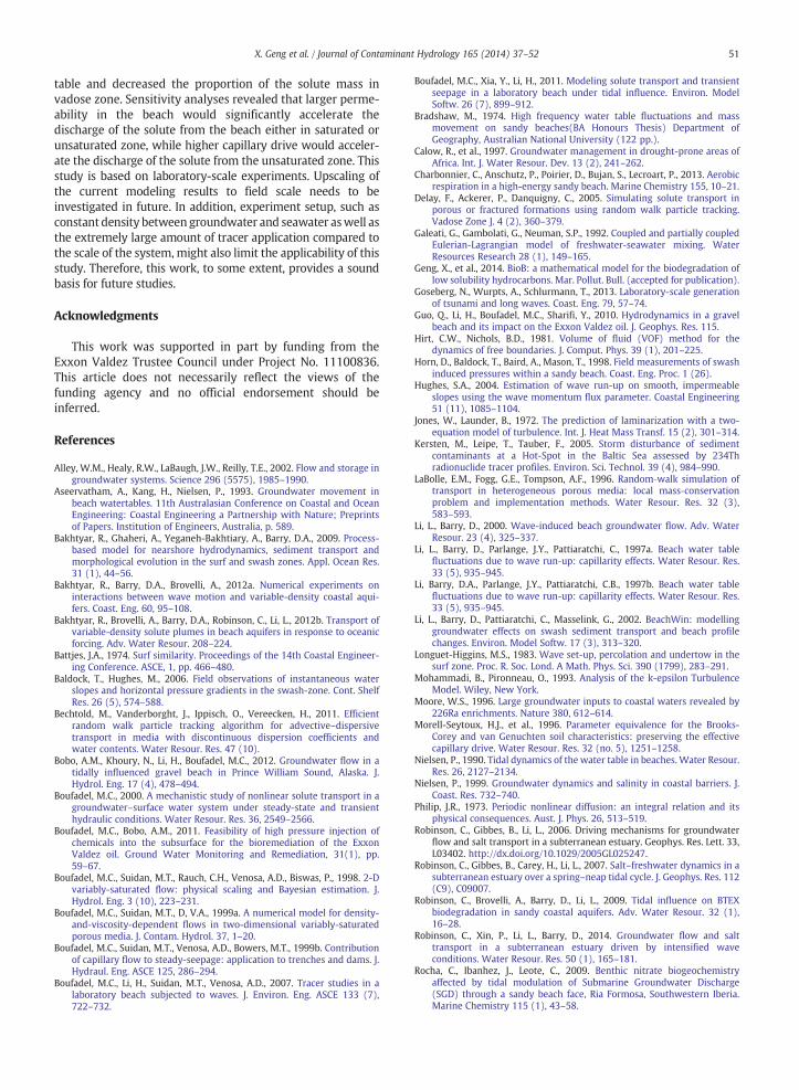
The trajectory of the plume centroid for different HcM
values is shown in Fig. 14a, which shows that the seawarddisplacement of the plume's centroid increased with HcM; in abeach with a large capillary fringe, due to higher moisturecontent, the solute in the unsaturated zone would movefaster seaward and thus discharge into the saturated zone
Fig. 13. Variation of normalized mass (current divided by that at 50 min) of the solute in the unsaturated and saturated zones of the beach as a function of time fordifferent effective capillary drive HcM (Eq. (17)). The larger HcM denotes the larger the capillary fringe. The upper panel reports the variation of the total mass inthe beach.
Fig. 14. (a) Trajectory of the plume centroid in the beach with differenteffective capillary drive HcM (Eq. (17)); (b) Variation of the area occupied bythe plume in the beach as a function of time for different values of HcM. Theedge of the plume is delineated by 10% of the maximum soluteconcentration (i.e., 0.27 g/L).
50 X. Geng et al. / Journal of Contaminant Hydrology 165 (2014) 37–52
closer to the discharge zone from the beach. The fact that thehorizontal transport in the unsaturated zone increases withthe capillary fringe was noted by Boufadel et al. (1999b) andBoufadel (2000). Fig. 14b shows the variation of the areaoccupied by the solute plume in the beach as function oftime. Increasing HcM resulted in a rapid decrease in the areafrom the maximum due to the larger hydraulic conductivity,as discussed above. However, the difference between theplume areas was small, indicating capillarity had less impacton the solute spreading area in comparison to permeability.
4. Conclusions
High-frequency waves are an important oceanic forcingaffecting groundwater flow and subsurface solute transportin coastal aquifers. In this paper, a numerical study wasconducted to investigate wave effects on groundwater flowand solute transport in a laboratory beach. The numericalsimulations revealed that waves induced seawater–ground-water circulations in the swash and surf zones of the beach,which generated a large seawater–groundwater exchangeacross the beach face. This effect increased the trajectorylength of subsurface solute transport and the residence timeof the plume. Residence Time Maps (RTM) revealed that thewave-induced residence time of the inland-applied soluteswas largest near the solute exit zone to the sea. Meanwhile,wave forcing accelerated the speed of solute movement inthe beach and intensified the mixing between plume andterrestrial groundwater near the beach face. The results alsosuggested that wave-induced seawater infiltration in swashzone increased the solute moving below the groundwater
51X. Geng et al. / Journal of Contaminant Hydrology 165 (2014) 37–52
table and decreased the proportion of the solute mass invadose zone. Sensitivity analyses revealed that larger perme-ability in the beach would significantly accelerate thedischarge of the solute from the beach either in saturated orunsaturated zone, while higher capillary drive would acceler-ate the discharge of the solute from the unsaturated zone. Thisstudy is based on laboratory-scale experiments. Upscaling ofthe current modeling results to field scale needs to beinvestigated in future. In addition, experiment setup, such asconstant density between groundwater and seawater aswell asthe extremely large amount of tracer application compared tothe scale of the system,might also limit the applicability of thisstudy. Therefore, this work, to some extent, provides a soundbasis for future studies.
Acknowledgments
This work was supported in part by funding from theExxon Valdez Trustee Council under Project No. 11100836.This article does not necessarily reflect the views of thefunding agency and no official endorsement should beinferred.
Aseervatham, A., Kang, H., Nielsen, P., 1993. Groundwater movement inbeach watertables. 11th Australasian Conference on Coastal and OceanEngineering: Coastal Engineering a Partnership with Nature; Preprintsof Papers. Institution of Engineers, Australia, p. 589.
Bakhtyar, R., Ghaheri, A., Yeganeh-Bakhtiary, A., Barry, D.A., 2009. Process-based model for nearshore hydrodynamics, sediment transport andmorphological evolution in the surf and swash zones. Appl. Ocean Res.31 (1), 44–56.
Bakhtyar, R., Barry, D.A., Brovelli, A., 2012a. Numerical experiments oninteractions between wave motion and variable-density coastal aqui-fers. Coast. Eng. 60, 95–108.
Bakhtyar, R., Brovelli, A., Barry, D.A., Robinson, C., Li, L., 2012b. Transport ofvariable-density solute plumes in beach aquifers in response to oceanicforcing. Adv. Water Resour. 208–224.
Battjes, J.A., 1974. Surf similarity. Proceedings of the 14th Coastal Engineer-ing Conference. ASCE, 1, pp. 466–480.
Baldock, T., Hughes, M., 2006. Field observations of instantaneous waterslopes and horizontal pressure gradients in the swash-zone. Cont. ShelfRes. 26 (5), 574–588.
Bechtold, M., Vanderborght, J., Ippisch, O., Vereecken, H., 2011. Efficientrandom walk particle tracking algorithm for advective–dispersivetransport in media with discontinuous dispersion coefficients andwater contents. Water Resour. Res. 47 (10).
Bobo, A.M., Khoury, N., Li, H., Boufadel, M.C., 2012. Groundwater flow in atidally influenced gravel beach in Prince William Sound, Alaska. J.Hydrol. Eng. 17 (4), 478–494.
Boufadel, M.C., 2000. A mechanistic study of nonlinear solute transport in agroundwater–surface water system under steady-state and transienthydraulic conditions. Water Resour. Res. 36, 2549–2566.
Boufadel, M.C., Bobo, A.M., 2011. Feasibility of high pressure injection ofchemicals into the subsurface for the bioremediation of the ExxonValdez oil. Ground Water Monitoring and Remediation, 31(1), pp.59–67.
Boufadel, M.C., Suidan, M.T., D, V.A., 1999a. A numerical model for density-and-viscosity-dependent flows in two-dimensional variably-saturatedporous media. J. Contam. Hydrol. 37, 1–20.
Boufadel, M.C., Suidan, M.T., Venosa, A.D., Bowers, M.T., 1999b. Contributionof capillary flow to steady-seepage: application to trenches and dams. J.Hydraul. Eng. ASCE 125, 286–294.
Boufadel, M.C., Li, H., Suidan, M.T., Venosa, A.D., 2007. Tracer studies in alaboratory beach subjected to waves. J. Environ. Eng. ASCE 133 (7),722–732.
Boufadel, M.C., Xia, Y., Li, H., 2011. Modeling solute transport and transientseepage in a laboratory beach under tidal influence. Environ. ModelSoftw. 26 (7), 899–912.
Bradshaw, M., 1974. High frequency water table fluctuations and massmovement on sandy beaches(BA Honours Thesis) Department ofGeography, Australian National University (122 pp.).
Calow, R., et al., 1997. Groundwater management in drought-prone areas ofAfrica. Int. J. Water Resour. Dev. 13 (2), 241–262.
Charbonnier, C., Anschutz, P., Poirier, D., Bujan, S., Lecroart, P., 2013. Aerobicrespiration in a high-energy sandy beach. Marine Chemistry 155, 10–21.
Delay, F., Ackerer, P., Danquigny, C., 2005. Simulating solute transport inporous or fractured formations using random walk particle tracking.Vadose Zone J. 4 (2), 360–379.
Galeati, G., Gambolati, G., Neuman, S.P., 1992. Coupled and partially coupledEulerian-Lagrangian model of freshwater-seawater mixing. WaterResources Research 28 (1), 149–165.
Geng, X., et al., 2014. BioB: a mathematical model for the biodegradation oflow solubility hydrocarbons. Mar. Pollut. Bull. (accepted for publication).
Goseberg, N., Wurpts, A., Schlurmann, T., 2013. Laboratory-scale generationof tsunami and long waves. Coast. Eng. 79, 57–74.
Guo, Q., Li, H., Boufadel, M.C., Sharifi, Y., 2010. Hydrodynamics in a gravelbeach and its impact on the Exxon Valdez oil. J. Geophys. Res. 115.
Hirt, C.W., Nichols, B.D., 1981. Volume of fluid (VOF) method for thedynamics of free boundaries. J. Comput. Phys. 39 (1), 201–225.
Horn, D., Baldock, T., Baird, A., Mason, T., 1998. Field measurements of swashinduced pressures within a sandy beach. Coast. Eng. Proc. 1 (26).
Hughes, S.A., 2004. Estimation of wave run-up on smooth, impermeableslopes using the wave momentum flux parameter. Coastal Engineering51 (11), 1085–1104.
Jones, W., Launder, B., 1972. The prediction of laminarization with a two-equation model of turbulence. Int. J. Heat Mass Transf. 15 (2), 301–314.
Kersten, M., Leipe, T., Tauber, F., 2005. Storm disturbance of sedimentcontaminants at a Hot-Spot in the Baltic Sea assessed by 234Thradionuclide tracer profiles. Environ. Sci. Technol. 39 (4), 984–990.
LaBolle, E.M., Fogg, G.E., Tompson, A.F., 1996. Random‐walk simulation oftransport in heterogeneous porous media: local mass‐conservationproblem and implementation methods. Water Resour. Res. 32 (3),583–593.
Li, L., Barry, D., Parlange, J.Y., Pattiaratchi, C., 1997a. Beach water tablefluctuations due to wave run‐up: capillarity effects. Water Resour. Res.33 (5), 935–945.
Li, Barry, D.A., Parlange, J.Y., Pattiaratchi, C.B., 1997b. Beach water tablefluctuations due to wave run-up: capillarity effects. Water Resour. Res.33 (5), 935–945.
Li, L., Barry, D., Pattiaratchi, C., Masselink, G., 2002. BeachWin: modellinggroundwater effects on swash sediment transport and beach profilechanges. Environ. Model Softw. 17 (3), 313–320.
Longuet-Higgins, M.S., 1983. Wave set-up, percolation and undertow in thesurf zone. Proc. R. Soc. Lond. A Math. Phys. Sci. 390 (1799), 283–291.
Mohammadi, B., Pironneau, O., 1993. Analysis of the k-epsilon TurbulenceModel. Wiley, New York.
Moore, W.S., 1996. Large groundwater inputs to coastal waters revealed by226Ra enrichments. Nature 380, 612–614.
Morell-Seytoux, H.J., et al., 1996. Parameter equivalence for the Brooks-Corey and van Genuchten soil characteristics: preserving the effectivecapillary drive. Water Resour. Res. 32 (no. 5), 1251–1258.
Nielsen, P., 1990. Tidal dynamics of the water table in beaches. Water Resour.Res. 26, 2127–2134.
Nielsen, P., 1999. Groundwater dynamics and salinity in coastal barriers. J.Coast. Res. 732–740.
Philip, J.R., 1973. Periodic nonlinear diffusion: an integral relation and itsphysical consequences. Aust. J. Phys. 26, 513–519.
Robinson, C., Gibbes, B., Li, L., 2006. Driving mechanisms for groundwaterflow and salt transport in a subterranean estuary. Geophys. Res. Lett. 33,L03402. http://dx.doi.org/10.1029/2005GL025247.
Robinson, C., Gibbes, B., Carey, H., Li, L., 2007. Salt–freshwater dynamics in asubterranean estuary over a spring–neap tidal cycle. J. Geophys. Res. 112(C9), C09007.
Robinson, C., Brovelli, A., Barry, D., Li, L., 2009. Tidal influence on BTEXbiodegradation in sandy coastal aquifers. Adv. Water Resour. 32 (1),16–28.
Robinson, C., Xin, P., Li, L., Barry, D., 2014. Groundwater flow and salttransport in a subterranean estuary driven by intensified waveconditions. Water Resour. Res. 50 (1), 165–181.
Rocha, C., Ibanhez, J., Leote, C., 2009. Benthic nitrate biogeochemistryaffected by tidal modulation of Submarine Groundwater Discharge(SGD) through a sandy beach face, Ria Formosa, Southwestern Iberia.Marine Chemistry 115 (1), 43–58.
52 X. Geng et al. / Journal of Contaminant Hydrology 165 (2014) 37–52
Rouxel, O., Sholkovitz, E., Charette, M., Edwards, K.J., 2008. Iron isotopefractionation in subterranean estuaries. Geochim. Cosmochim. Acta 72(14), 3413–3430.
Santas, R., Santas, P., 2000. Effects of wave action on the bioremediation ofcrude oil saturated hydrocarbons. Mar. Pollut. Bull. 40 (5), 434–439.
Schulz, H.D., 2000. Quantification of early diagenesis: dissolved constituentsin marine pore water. Mar. Geochem. 85–128 (Springer).
Sous, D., Lambert, A., Vincent, R., Michallet, H., 2013. Swash–groundwaterdynamics in a sandy beach laboratory experiment. Coast. Eng. 80,122–136.
Tompson, A.F., 1993. Numerical simulation of chemical migration inphysically and chemically heterogeneous porous media. Water Resour.Res. 29 (11), 3709–3726.
Turner, I.L., Masselink, G., 1998. Swash infiltration‐exfiltration and sedimenttransport. J. Geophys. Res. Oceans (1978–2012) 103 (C13), 30813–30824.
van Genuchten, M.T., 1980. A closed-form equation for predicting thehydraulic conductivity of unsaturated soils. Soil Sci. Soc. Am. J. 44 (5),892–898.
Voss, C.I., Souza, W.R., 1987. Variable density flow and solute transportsimulation of regional aquifers containing a narrow freshwater–saltwater transition zone. Water Resour. Res. 23 (10), 1851–1866.
Wilcox, D.C., 1998. Turbulence Modeling for CFD, 2. DCW industries LaCanada, CA.
Xin, P., Robinson, C., Li, L., Barry, D.A., Bakhtyar, R., 2010. Effects of waveforcing on a subterranean estuary. Water Resour. Res. 46 (12).
Zghibi, A., Zouhri, L., Tarhouni, J., Kouzana, L., 2012. Groundwatermineralisation processes in Mediterranean semi‐arid systems (Cap‐Bon, North east of Tunisia): hydrogeological and geochemical ap-proaches. Hydrol. Process. 27 (22), 3227–3239.