http://eng.sagepub.com Journal of English Linguistics DOI: 10.1177/0075424205279017 2005; 33; 99 Journal of English Linguistics Robert G. Shackleton, JR. English-American Speech Relationships: A Quantitative Approach http://eng.sagepub.com/cgi/content/abstract/33/2/99 The online version of this article can be found at: Published by: http://www.sagepublications.com can be found at: Journal of English Linguistics Additional services and information for http://eng.sagepub.com/cgi/alerts Email Alerts: http://eng.sagepub.com/subscriptions Subscriptions: http://www.sagepub.com/journalsReprints.nav Reprints: http://www.sagepub.com/journalsPermissions.nav Permissions: http://eng.sagepub.com/cgi/content/refs/33/2/99 Citations at University of Groningen on September 1, 2009 http://eng.sagepub.com Downloaded from
Transcript
http://eng.sagepub.com
Journal of English Linguistics
DOI: 10.1177/0075424205279017 2005; 33; 99 Journal of English Linguistics
Robert G. Shackleton, JR. English-American Speech Relationships: A Quantitative Approach
http://eng.sagepub.com/cgi/content/abstract/33/2/99 The online version of this article can be found at:
Published by:
http://www.sagepublications.com
can be found at:Journal of English Linguistics Additional services and information for
This study applies quantitative techniques—measures of linguistic distance, cluster analy-sis, principal components analysis, and regression analysis—to data on English speech vari-ants in England and America. The analysis yields measures of similarity among English andAmerican speakers, distinguishes clusters of speakers with similar speech patterns, and iso-lates groups of variants that distinguish those groups of speakers. The results are consistentwith a model of new-dialect formation in the American colonies, involving competitionwithin and selection from a pool of variants introduced by speakers from different dialect re-gions. The patterns of similarity appear to be largely consistent with the historical evidenceof migrations from seventeenth- and eighteenth-century Britain to North America, lendingsupport to the hypothesis of regional English origins for some important differences inAmerican dialects, and suggesting mainly southeastern English influence on Americanspeech, with somewhat greater southeastern influence on New England speech andsouthwestern influence in the American South.
Keywords: English dialect; American dialect; dialectometry; historical dialectology
Linguists and layfolk alike have devoted much thought to the origins of Ameri-can English dialect forms. Some have emphasized the importance of non-Europeanand non-English influences on the development of American speech. Others stresscontinuities with traditional English forms from various parts of the British Isles,even arguing that “some of today’s most noticeable dialect differences can betraced directly back to the British dialects of the seventeenth and eighteenth centu-ries.”1 The latter view underlies such efforts as that of Cleanth Brooks (1935), whoundertook a detailed review of the British dialect material in Joseph Wright’s Eng-lish Dialect Dictionary (1898-1905), systematically comparing more than onehundred forms found in the speech of his native region of Alabama (or used by
AUTHOR’S NOTE: The author gratefully thanks William Kretzschmar, Salikoko Mufwene, and JohnNerbonne for extremely helpful guidance and advice in the conduct of this work; Crawford Feagin for in-sightful comments on a very early version of this article; William Labov for the questions that inspiredthe principal components analysis; and two anonymous reviewers who provided very useful criticisms ofan earlier draft. The analysis and conclusions expressed in this article are those of the author and shouldnot be interpreted as those of the Congressional Budget Office.
characters in southern American literary works) with forms found in different partsof England. Brooks concluded that southern American speech forms were derivedprimarily from earlier dialects spoken mainly in southern England, particularly insouthwestern England.
An important development in dialect research occurred three years later when,in conjunction with his research for the Linguistic Atlas of New England (LANE)(Kurath, 1939) and the Linguistic Atlas of the Middle and South Atlantic States(LAMSAS), Guy Lowman conducted a wide-meshed survey of rural speech insouthern England to permit more informed comparisons between the speech formsof England and America than had been possible previously. After Lowman’s un-timely death in 1941, the materials from his English survey were interpreted andpresented by others. Viereck (1975) described extensive lexical and grammaticalresults as well as much of the supporting methodological detail, and in The DialectStructure of Southern England, Kurath and Lowman (1970) summarized the pho-nological material, presented some tentative conclusions about the structure ofsouthern English dialects, and noted some correspondences between southernEnglish forms and those found in different regions of the United States.
In The Pronunciation of English in the Atlantic States, Kurath and McDavid(1961) published even more phonological detail from Lowman’s English research,presenting results from LANE, and LAMSAS, and his survey in a series of annotatedmaps illustrating the occurrence of different variants of English phonemes in theAtlantic states as well as in southern England. The maps reveal a great variety offorms in both England and America during the first half of the twentieth century.Even though the maps are not based on any systematic quantitative assessment orcomparisons, they clearly illustrate that most variants found in use by Americanspeakers could also be found in use by traditional southern English speakers, al-though American speech was considerably less variable than that of rural southernEngland.
During the past two generations, researchers have continued to uncover sourcesof American speech forms from southern England and elsewhere. Recently, for ex-ample, Montgomery (2001) traced the influence—predominantly on vocabulary—of eighteenth-century Scots-Irish immigrants on speech in the Appalachiansand Upper South. Wright (2003) uncovered a variety of grammatical features asso-ciated with Southern American English in prisoners’ narratives from early-seventeenth-century London. Algeo (2003, 9), discussing the origins of SouthernAmerican English, argued for “multiple lines of descent” from southern and west-ern English, Scotch-Irish, African, and other influences. Orton and Dieth (1962)have also improved on Lowman’s English research by completing and publishing aSurvey of English Dialects, covering all of England.
Historians, too, have contributed to linguistic research by tracing differences inthe British origins of settlers of different regions of North America. Notable exam-
100 JEngL 33.2 (June 2005)
at University of Groningen on September 1, 2009 http://eng.sagepub.comDownloaded from
ples are Bailyn (1986) and Fischer (1989), who documented extensive processes ofinternal migration from all over the British Isles to London and a predominance ofemigration to most of the colonies from London and surrounding regions. How-ever, both sources also show somewhat greater than average migration from EastAnglia to New England, from the Midlands to Pennsylvania, from the West Coun-try to Virginia, and from Scotland and northern Ireland to the backcountry.
A related strand of research, one that benefits from the more recent nature of thephenomena in question and, consequently, greater availability of data, focuses onthe development of English dialects in other, more recently settled colonies such asAustralia and New Zealand. Trudgill (1986, 142) compared a number of phoneticcharacteristics of Australian English with those of English dialects, noting a veryclose relationship between Australian English and the speech forms of London andEssex, and concluded that Australian English is “a mixed dialect which grew up inAustralia out of the interaction of south-eastern English forms with East Anglian,Irish, Scottish and other dialects.” More recently, Trudgill (2004, 2) has closelystudied the process of new-dialect development following contact among speakersof different dialects of English, noting that such contact “would have led to the ap-pearance of new, mixed dialects not precisely like any dialect spoken in the home-land.” In the case of New Zealand, Trudgill tracked the process of dialect formationfrom a first stage of dialect contact among immigrants from a variety of British ori-gins, through a second stage in which first-generation speakers choose from the va-riety of speech forms available to them, to a third stage in which a relatively uniformdialect emerges among second-generation speakers.
From such strands of research, many dialectologists conclude that differences inmigration patterns and settlement histories are likely to have contributed to signifi-cant differences among American regional dialects, with a largely but not exclu-sively English influence. The processes that led to such differentiation were pre-sumably as complex as those documented by Trudgill (2004) for New Zealand.They were likely driven in part by what Mufwene (1996) has called the founder ef-fect, by which the speech forms of the earliest settlers have an inherent advantage inthe process of survival and propagation, analogous to the biological advantage oftheir genes. In addition, several other processes may be hypothesized and in somecases documented. Through a constant process of speakers adapting their speechhabits to those of their most frequent interlocutors, variants most frequently usedby the largest group of settlers were probably more likely to dominate. Some vari-ants may have acquired higher prestige and spread; others may have been stigma-tized and therefore declined. Speakers may have come to associate particular vari-ants with ethnic or regional identities, tying the fate of those variants with that of theidentities. Kretzschmar (2002) emphasized that the processes were largely local,noting that despite the development of American forms of English that appeared re-markably uniform to many British observers, records of colonial speech patterns
reveal a great deal of regional and even local diversity, belying any simple narrativeinvolving the emergence of regional dialects from a melting, mixing, or weaving offorms brought during settlement.
Until recently, many experts had concluded not only that differences amongAmerican regional dialects were largely the result of settlement processes but thatmany if not most regional differences in the Atlantic States were largely formed bythe American Revolution. More recent research has emphasized the importance ofinnovations that occurred after the period of colonization and settlement. Schneider(2003), examining Orton, Sanderson, and Widdowson (1978) for possible Englishsources of twenty-five pronunciation features common in Southern American Eng-lish, has found eleven in southwestern England and eight in the southeast (with con-siderable overlap), but only four to five in other regions. Schneider concluded thatthere is some “limited continuity of forms derived from British dialects” but “also agreat deal of internal dynamics to be observed . . . and . . . strong evidence for muchinnovation” (p. 34). Similarly, linguists such as Bailey (1997), while accepting thatfeatures of colonial and early postcolonial varieties were likely largely a conse-quence of settlement history, have shown that some common Southern AmericanEnglish features (such as the pin/pen merger) that may have been in sporadic usenot long after the Revolution did not become common until long after the period ofsettlement.
In the meantime, linguists have made significant progress in a complementarystrand of research, the development of methods of quantifying differences amongspeech forms.2 Moving well beyond the isogloss methods characteristic of earlierwork, this research has provided a variety of methods of measuring distances be-tween sound segments, either measured acoustically or, as in the case of theLowman data, impressionistically, as well as methods to measure distances be-tween speakers or groups of speakers, based on aggregates of measures betweenspecific sound segments. Dialectologists have employed such tools to great effect,as for example in Heeringa’s (2004) analysis of Dutch and Norwegian dialects orNerbonne’s (2005) examination of American speech in Virginia and NorthCarolina.
To date, however, no such dialectometric analysis has been applied to a data setincluding both English and American speakers. An effort to quantify linguistic dis-tances among English and American speech forms and speakers recorded in thetwentieth century may provide some insights into how varieties of American Eng-lish have developed over time, and perhaps even how English variants were se-lected in the process of new-dialect development in the American colonies. Such aneffort is hampered, of course, by time distance: the fact that the earliest English set-tlers arrived nearly four centuries ago raises serious questions as to whether asynchronic comparison of twentieth-century American and English forms can pro-vide any insights at all into dialect developments during colonization. However, the
102 JEngL 33.2 (June 2005)
at University of Groningen on September 1, 2009 http://eng.sagepub.comDownloaded from
barrier may not be quite as profound as it seems at first sight: parts of the Atlanticcoast were still being settled at the end of the seventeenth century, and some of thespeakers interviewed by Lowman were born in the middle of the nineteenth cen-tury. In at least some cases, therefore, the time distance is more like 150 years ratherthan 400 years—enough distance to raise questions as to whether the proposedcomparisons can yield historical insights, certainly, but not enough distance topreclude the possibility altogether.
This study discusses characteristics of the data presented in Kurath andMcDavid (1961) and Kurath and Lowman (1970) discussed above, and appliesquantitative techniques to that data to characterize the degrees and patterns of simi-larity among a subset of American and English speakers, to distinguish clusters ofspeakers with similar speech patterns, and to isolate groups of variants that distin-guish those groups of speakers. The results provide insights into the differences andsimilarities among dialects and can be used to make tentative inferences about theprocesses of new-dialect formation that might have occurred in the development ofAmerican regional dialects.
Assembling Data from Kurath and McDavid’s (1961)Pronunciation of English in the Atlantic States and Kurath and
Lowman’s (1970) Dialect Structure of Southern England
In an ideal world, this analysis would draw on easily accessible and interpretabledata, preferably collected by one person using a uniform methodology, describingas many speech forms as possible from informants from different regions. The realdata that best (though quite imperfectly) meet those criteria appear to be those pre-sented in the maps of two works: Kurath and McDavid’s (1961) Pronunciation ofEnglish in the Atlantic States (henceforth PEAS) and Kurath and Lowman’s (1970)Dialect Structure of Southern England (DSSE). Figure 1, taken from PEAS, showsa sample of that data: a map of the occurrence of six different vocalic variants usedin care, each variant distinguished by a different type of marker. Each marker repre-sents the pronunciation of a specific informant from a given location, althoughthere are often two or more informants from a location, occasionally more than onevariant per informant, and occasionally no data for an informant. Kurath andMcDavid sometimes distinguished regions in which a particular variant was wide-spread by using a large marker (the large black triangles in New England, for in-stance), indicating the occurrence of other variants with regularly sized markers. Itis usually rather easy to associate a marker with an informant described in Kurath(1939)—the LANE handbook—or Kretzschmar et al. (1994)—the LAMSAS hand-book—or Viereck (1975), which describes Lowman’s English informants. Themarkers, however, were not always placed in exactly the same place on each map,and the interpretive process occasionally becomes somewhat creative.
Altogether, eighty-four maps in PEAS provide information about 275 phoneticvariants recorded in 76 different words (or, in one case, a phrase) in England andAmerica. Two of the maps also permit us to distinguish between informants whoshow a single pronunciation for the vowel in words pronounced with [a·] or [ai] inLondon standard Middle English and those who do not. In addition, six maps ofLowman’s English data in DSSE provide data that can be used to tabulate the south-ern English usage of variants in one or more words or to distinguish a merger (Mid-dle English [ou] and [O·]). For one of those words, maps from PEAS provide the
104 JEngL 33.2 (June 2005)
Figure 1: Annotated Map from Kurath and McDavid (1961) Showing the Location of American andEnglish Informants and Regions. Reprinted with permission from The Pronunciationof Eng-lish in the Atlantic States, by Hans Kurath and Raven I. McDavid, Jr., University of MichiganPress, 1961.
at University of Groningen on September 1, 2009 http://eng.sagepub.comDownloaded from
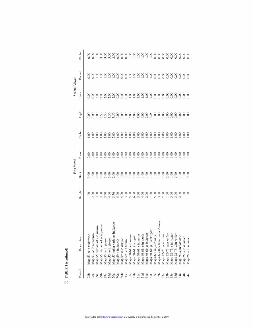
American usages; for the others, Americans universally have a single, obvious us-age (for example, unvoiced fricatives in words like furrow, fog, and frost). Alto-gether, the maps in PEAS and DSSE make it possible to distinguish and tabulate theEnglish and American informants’ usage of 284 variants in 81 different words—many of which are particularly notorious for a variety of nonstandard pronunciations—and the presence or absence of two mergers. The words cover nearly all phonemesin standard British English and American English (unstressed, short, and long vow-els; diphthongs [including many rhotic ones]; and a number of consonants) usuallywith 1 to 4 words for a particular phoneme but with 5 or more words for a few. Thefull list—83 cases involving a total of 288 variants (including the mergers), asshown in Table 1—constitute a fairly wide if not fully comprehensive tabulation ofphonetic variation in southern English and American speech.
A few qualifications are in order. First, in considering the utility of this data setfor comparing speech forms, it is important to keep in mind that the detailed re-sponses recorded by the interviewers were grouped into variants or “allophones”by Kurath and McDavid, causing a significant loss of real diversity in the character-izations used here. In this sense, some of the variability in the data has already beeneliminated by Kurath and McDavid’s choices of how to classify responses into vari-ants. The choices reflect those researchers’ views of the structure of English dia-lects, and as a consequence their views may well be reflected in any results derivedfrom analysis of the data. Second, in several cases the nature of the data requires usto create a residual variant that in fact constitutes a group of variants that cannot bereadily distinguished. In those cases, too, the data (and any analysis of it) tends tounderstate the actual variability of the speech forms. Third, in a few cases, the rep-resentation of the data on the maps makes it very difficult to determine which of twoor three possible informants in a given locality gave the observation; in these cases,the attribution is made arbitrarily. All three of those limitations could be overcomeby future research drawing from the interviewers’ original records.
A further qualification is that in a handful of cases, mainly in maps from DSSE,the maps present data that is more in the nature of a frequency (e.g., the presence ofa variant in one or more of six words) than nominal data indicating simple presenceor absence of a variant in a single word. As a general rule it is inadvisable to mixnominal data and frequency data. In the case of the Lowman data, however, it doesnot appear to be a gross violation of that rule to interpret the nominal data as 0 per-cent or 100 percent frequency usage of a particular variant in a specific context by aspecific informant, and to combine it with data that measures 0 percent to 100 per-cent frequency of a particular variant in several contexts by the same informant.
Because this analysis is focused primarily on the transmission of speech formsduring the early settlement of the English colonies, it draws from the maps to obtainrecords only for informants from England and from three relatively restricted areas
in the United States. (Obviously, a great deal more insight may be gleaned by ex-panding the analysis to include records from more of the American informantsrepresented in PEAS.) The analysis includes records for informants in two Ameri-can regions that were settled extremely early: twenty-two informants in a regionsurrounding Plymouth, Massachusetts, and thirty-one informants in a region alongthe southern Virginia and northern North Carolina coast (see Figure 1). In addition,the analysis includes records for nineteen informants from a region encompassingsouthernmost West Virginia and southwestern Virginia, the geographic gateway ofCarver’s (1987) Upper South dialect region. That latter choice reflects the author’sparticular interest in understanding the origins of Appalachian speech and in test-ing the popular perception that because Appalachian speakers are particularlyisolated, they retain archaic speech forms to a greater degree than do speakers ofmany other dialects.
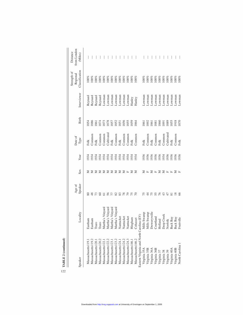
Table 2 presents information describing the informants and their interviews.3
Guy Lowman interviewed most but, unfortunately, not all of the informants: seveninformants in southeastern England were interviewed by Henry Collins, thirteen ofthe informants in Massachusetts were interviewed by Cassil Reynard, and twomore were interviewed by Miles Hanley. Most of the interviews were conductedbetween 1934 and 1940, with the exception those done by Collins, which were con-ducted in 1950. All but two of the English informants whose gender can be identi-fied from the records were male, so chosen, presumably, on the principle that mentend to retain more old-fashioned speech forms. All of the English informantscould be classified as older “folk” speakers of traditional rural dialects—that is,speakers with “local usage subject to a minimum of education and other outside in-fluence” (Kretzschmar et al. 1994, 25). In most cases we know only that they weregenerally over the age of sixty, and therefore typically born before 1878.
The directors of the Linguistic Atlas projects attempted to secure a representa-tive cross-section of regional speech forms acquired mainly during the second halfof the nineteenth century, with moderate but not exclusive emphasis on folk speech.In the regions examined in this study, all of the American informants were white;nearly all lived in rural settings or in small towns and came from families that werelong established in the region. All but one of the Massachusetts informants—butonly twenty-six of the fifty southern American informants—were male. The inter-viewers classified more than half (thirty-nine, or 54 percent) of the American infor-mants as folk speakers. They classified twenty-seven (38 percent) as “common”speakers with “local usage subject to a moderate amount of education . . . privatereading, and other external contacts” and the remaining six (8 percent) as “culti-vated” speakers with “wide reading and elevated local cultural traditions, generallybut not always with higher education” (Kretzschmar et al. 1994, 25). The typical
118 JEngL 33.2 (June 2005)
(text continues on page 125)
at University of Groningen on September 1, 2009 http://eng.sagepub.comDownloaded from
American speaker was born in 1872 and was sixty-four years old at the time of theinterview. The youngest was born in 1918 and was eighteen, and the eldest wasborn in 1846 and was eighty-eight.
To summarize, data for each of the fifty-nine English and seventy-two Americaninformants are represented by a vector of 288 variables. Most take a value of 1 or 0,indicating the informant’s use or lack of use of a particular variant. In a handful ofcases, the value indicates the frequency with which the informant uses the variant ina set of words. The interviewers occasionally elicited more than one variant per in-formant, in which case both are represented in the data set. Less than 2 percent ofthe data are missing, where interviewers did not ask a question or did not get a use-ful reply. More than a third of the observations are missing no data, and only a hand-ful are missing more than 5 percent. The data set is available as a Microsoft Excelspreadsheet on request from the author.
Choice of Quantitative Techniques
A variety of quantitative techniques can be brought to bear to analyze the varia-tion in the sample and the degree of similarity among speakers within and amongregions, to distinguish groups of speakers with similar speech patterns, and to dis-tinguish groups of variants that characterize those groups’ speech patterns. Manysuch methods have already been applied in studies of dialect geography but not, tomy knowledge, to phonetic data from PEAS and DSSE. In this study, I present theanalysis in the following sequence:
• Using cluster analysis to find dialect regions. A variety of clustering techniques can beused to group informants on the basis of some measurement of similarity of theirspeech patterns. Ideally, the groups will be interpretable as geographically contiguousdialect regions. By distinguishing a reasonably coherent set of dialect regions, the clus-ter analysis lays the basis for examining the geographic distribution of variants and formeasuring degrees of similarity among speakers from different regions.
• Analyzing the distribution of variants. A great deal can be learned by simply examininghow variants are distributed among speakers in different regions—how many (andwhich) variants appear in different regions, and how many are shared between andamong regions.
• Applying measures of similarity (distance measures) among informants. Even more in-formation can be uncovered by measuring degrees of similarity between and among in-dividual speakers within and among regions. By helping to distinguish degrees of dif-ference among varieties of speech, distance measures provide a reasonably objectivegauge of whether (and which) English and American informants’ speech forms are dra-matically different or relatively similar. A number of measures are available, includingthe percentage of a speaker’s total number of variants that he or she shares in commonwith other speakers; Pearson correlations, Euclidean distances, or cosines betweenvectors of values of variants; and various measures of linguistic distance or genetic dis-tance. The analysis presented in this article focuses on the simplest of these measures—
the percentage of shared variants—and on a quantitative measure of the articulatory oracoustic differences between speakers’ variants: that is, a measure of linguistic dis-tance, which is arguably most appropriate to the data. (The cluster analysis discussedabove and the principal components analysis discussed below rely on other measures,discussed in the following sections.)
• Principal components analysis. With data sets that measure variation along a largenumber of dimensions (such as the occurrence, nonoccurrence, or frequency of occur-rence of variant pronunciations), principal components analysis can be used to reducethe information to a smaller number of dimensions that, ideally, have clear interpreta-tions. In this case, principal components analysis can be used to determine whether(and how strongly) groups of variants tend to occur together and whether (and what)groups of speakers use those groups of variants together. Ideally, the principal compo-nents that are the output of such an analysis will be interpretable as linguistically rele-vant groups of variant pronunciations and will have clear interpretations in terms ofdialect geography.
• Multiple regression analysis. Finally, regression analysis can be used to test for rela-tionships between variables and may provide insights into geographical characteristicsof the distribution of variants. In this case, I use regressions to test for a statistically sig-nificant relationship between the degree of similarity between English and Americanspeakers and the proximity of the English speakers to London. Such a relationship, if itexists, may provide support for the hypothesis that speech in or near the London metro-politan area played a key role in the development in American speech varieties.
The techniques used in this study are implemented using either the Statistical Pack-age for the Social Sciences (SPSS) for Windows Version 7.5 or a Fortran-basedprogram written by and available on request from the author.
Using Cluster Analysis to Distinguish Dialect Regions
Cluster analysis refers to a large set of mathematical procedures that divide datainto classes based on relationships within the data, thus dramatically reducing vari-ation along a number of dimensions in the data set to a single set of clusters.4 In thisstudy, clustering methods are used to classify informants whose speech is similaraccording to some quantitative measure into distinct groups.
Clustering techniques include nonhierarchical methods, in which the data aredivided into an arbitrary number of classes and each observation is assigned to aparticular class, and hierarchical methods, in which classes may be divided intosubclasses. Nonhierarchical methods exclude any relation among clusters, whilehierarchical methods allow subclusters to be more or less closely related as mem-bers of larger clusters, and a given observation may be a member of severalsubclusters—for example, a large cluster of clusters, one of that group’ssubclusters, and so on (hence the notion of hierarchy). Hierarchical methods in-clude divisive techniques, which divide and subdivide a data set into subsets untilsome predetermined limit is reached, and agglomerative methods, which start with
126 JEngL 33.2 (June 2005)
at University of Groningen on September 1, 2009 http://eng.sagepub.comDownloaded from
each observation as a separate cluster, join the most similar ones, and continue tojoin the resulting clusters until all clusters have been united.
Every clustering method and distance measure has strengths and weaknesses,depending on the actual distribution and type of the data. This analysis tries to com-pensate for the weaknesses of different methods and measures by using several ofeach. First, it applies a nonhierarchical clustering method and a Euclidean distancemeasure to explore how the speakers cluster as the number of clusters is increasedfrom two to ten. Second, it applies twelve different hierarchical analyses, using fourdifferent agglomerative methods—single linkage (nearest neighbor), completelinkage (furthest neighbor), average linkage between groups, and average linkagewithin groups—and three different distance measures—Euclidean distances,Pearson correlations, and cosines.5 The multiplicity of approaches helps provideinsights into the robustness of the clusters produced under different approaches.
Nonhierarchical clustering reveals several interesting patterns as the number ofclusters arbitrarily imposed increases from two to eight:
• With two clusters, all of the English informants separate into one cluster and all of theAmerican informants into the other.
• With three clusters, the informants from the west and parts of the southeast of Englandform a cluster, and the southern American informants form another. The remainingcluster is composed of informants from the East Midlands, East Anglia, Middlesex,and Massachusetts.
• With four clusters, all of the Americans regroup into a single cluster, while the Englishinformants split into three clusters: an eastern group including East Anglia, part ofMiddlesex, and parts of the East Midlands; a more central group that includes the rest ofthe East Midlands and the southeast; and a western group.
• With five clusters, the Massachusetts informants and the American southerners formseparate and distinct groups, and remain so in subsequent clustering—all furtherreconfigurations involve only the English informants. The eastern English group fromthe previous clustering expands to include members of the central group, which shrinksaccordingly to include mainly only southeastern informants. The western groupremains unchanged.
• With six clusters, the expanded eastern English cluster splits in two, yielding a mainlyEast Anglian cluster and another encompassing most of the East Midlands. The south-eastern and western groups remain essentially unchanged.
• With seven clusters, the two Devonshire informants split out into a single group, leav-ing the rest of the clusters largely unchanged from the previous pattern with sixclusters.
• With eight clusters, three informants from Lincolnshire and Rutland form a separategroup distinct from a larger East Midlands group, into which the Middlesex informantsmove. The remaining East Anglian and southeastern informants form two distinctgroups. The large western group breaks into northern and southern clusters, with theDevonshire informants, previously separate, joining the northern (or West Midlands)cluster.
Hierarchical analysis of the data set yields further insights. Typically, the choiceof method has more effect on the clustering than the distance measure; differentclustering methods can yield quite different groupings, while different distancemeasures often yield rather similar ones. All approaches cluster the Massachusettsinformants into a single cluster and the southern American informants into another.The southern American cluster often divides into two or three subclusters, andthose subclusters tend to divide along regional lines: that is, one cluster will tend tobe composed mainly of informants from West Virginia and southwestern Virginia,while the other(s) will tend to be composed mainly of informants from eastern Vir-ginia and North Carolina. However, in every such case some westerners clusterwith easterners and vice versa, with no obvious pattern involving gender, age, ortype of speech.
Nine of the twelve hierarchical analyses—all except those using the single-linkage method—place the Massachusetts and southern American clusters in alarger cluster that includes most of the eastern English informants, while the west-ern English informants form a separate broad cluster. Under most of those ap-proaches, the Americans form a separate large subcluster and the eastern Englishinformants form a separate subcluster, which is itself divided into a number ofsubclusters—usually three. In a few cases, one or another American group clusterswith one or another of the eastern English subclusters. Using one method—averagelinkage within groups—and using any of the three distance measures, the south-eastern English subcluster groups together with the southern Americans.
The eastern English informants tend to divide into three subclusters under mostapproaches: a group mainly including informants from the East Midlands and thearea to the north of London, another mainly composed of East Anglians, and thelast centered in the counties southeast of London, but tending to include a handfulof informants north and west of London. The western English tend to divide intotwo groups, one composed of informants from the southwestern coastal countiesand the other including most of the informants to the north and west of London. Al-though the southwestern coastal informants form a stable group, the other cluster israther unstable: under almost every approach, at least some of the more northerlywesterners cluster into the coastal group, but which ones do so varies by approach.The most westerly informants, in Devonshire, sometimes cluster into the coastalgroup, sometimes into the more northerly group, sometimes by themselves as anoutlier cluster, and under one clustering method, along with the southeasterners andAmerican southerners. Using the single linkage approach, the westerners form asingle large cluster with no distinctive subclusters, except for the Devonshire infor-mants, who form an outlier cluster distinct from all other English and Americanspeakers.
Taken together, the clustering process thus yields a great deal of informationabout the similarity of informants among regions. Southern England has two broad
128 JEngL 33.2 (June 2005)
at University of Groningen on September 1, 2009 http://eng.sagepub.comDownloaded from
groups of dialects, one eastern and one western. American speakers are clearly dis-tinct from most southern English speakers, but they appear to have more in com-mon with eastern English speakers than western ones. The American southernersform a distinct group that, compared with the southern English speakers, is so uni-form that speakers from the North Carolina coast can hardly be distinguished fromthose in southern West Virginia. East Anglians form a largely distinct group; speak-ers in the East Midlands form another, and speakers in the southeast yet another.Speakers from near London appear to have affinities with those of the southeast butalso with those of the East Midlands. Southeastern speakers seem to be situated be-tween east and west, linguistically speaking, but closer to the east. Western Englishspeakers may be thought of as forming three rather indistinct groups, one inDevonshire, a more distinct one along the south coast, and a third making up thesouthwest Midlands—the Cotswolds and the Upper Thames and Severn Valleys.
Drawing on all twelve approaches and using majority (or, where necessary, plu-rality) rule, I assign the southern English informants to the six regions shown in Ta-ble 2 and delineated in Figure 1: the East Midlands (EM), East Anglia (EA), theSoutheast (SE), the Southwest (SW), Devonshire (DV), and the West Midlands(WM). The regions broadly correspond to the dialect regions noted by Kurath andLowman (1970) and are also largely congruent with the dialect regions delineatedin Trudgill (1990) as well as with the dialect clusters that the author has found in un-published cluster analyses of data from Orton and Dieth (1962).
The second-rightmost column of Table 2 provides a measure of how often infor-mants cluster into their designated region under the approaches used here. Whilemost informants in most English regions always cluster into the designated region,nearly every region has several informants that appear only loosely connected to it.For instance, the most northerly informant—designated “Lincolnshire 1”—isclearly more like an East Midlands speaker than like those of any of the other re-gions in the analysis, but he is really a North Midlands speaker and thus tends to ap-pear as an outlier under most approaches. (Under a few approaches he even clustersas an outlier in the Massachusetts group.) The regional classification of several in-formants near the borders of regions (especially near London, in Middlesex, Hart-ford, and Essex) is quite sensitive to the choices of approach and distance measure.That suggests that the regions are best thought of as rather loosely bounded: speak-ers appear to inhabit a linguistic continuum as much as they do a set of sharply dis-tinct dialect regions. Indeed, informants at the borders of regions occasionally areclassified into American groups, bringing to mind the hypothesis that like the bor-der informants, American speakers may best be thought of as having characteristicsof several of the English regions.
Note also that London itself emerges as a center surrounded by rather differentdialect regions. As shown in the last column of Table 2, with the exception ofDevonshire, every one of the regions assigned in the analysis has at least one infor-
mant within forty miles of London. Even at such close distances, however, the Eng-lish speakers tend to cluster rather regularly into separate clusters rather than into ametropolitan cluster, suggesting that the very extensive and protracted historicalmigrations from all over the British Isles to London had relatively little effect on thespeech patterns of rural speakers in the surrounding region.6
Analyzing the Distribution of Variants within and among Regions
A few simple summary measures describing the distribution of variants amongregions provide a remarkably clear picture of the extensive variation within andamong regions and overlap across regions. Of the total of 288 different variantsfound in the sample, 91 percent were found somewhere in southern England; 20percent are found only in southern England and are absent in the American regions.These two statistics alone imply that 22 percent of the variants found in southernEngland were not transplanted to (or were lost in) the American regions, suggestinga significant amount of leveling in the development of American regional speechforms.
Similarly, 80 percent of the variants were found in one or more of the Americanregions, while only 9 percent were found only in America. Thus, the overwhelmingmajority of American variants were clearly also native to southern England even inthe twentieth century. The fact that about 12 percent of American variants were notfound in southern England by Lowman may be taken to indicate some degree of in-novation in America, but that conclusion should be tempered by the observationthat many of the apparent innovations are known to have existed in southern Eng-land in earlier periods or were found somewhere in England by other twentieth-century fieldworkers such as those from the Survey of English Dialects (Orton andDieth 1962). Moreover, the fact that fully half of the apparent innovations areshared across all three American regions further suggests that they could very wellhave been in the inventory of speech forms imported to America.
Table 3 shows the percentages of the total population of variants found in eachregion and the percentages shared between regions. For example, the first numberin the first column of Table 3 shows that 74.3 percent of all variants were found inuse in the East Midlands (EM), each by at least one informant; the third numberinforms us that 49.0 percent of all variants were found both in the East Midlandsand in the Southeast (SE), and the seventh number (like the first number in the sev-enth column) reveals that 48.3 percent of them were found both in the East Mid-lands and in Massachusetts (MA).
In contrast, Table 4 shows, by column, the percentages of a given region’s totalvariants that it shares with each other region (that is, the numerator of every value ina column in Table 4 is the total number of variants found in the specified region).The seventh number of the first column of Table 4 thus shows that the variants
130 JEngL 33.2 (June 2005)
at University of Groningen on September 1, 2009 http://eng.sagepub.comDownloaded from
shared between the East Midlands and Massachusetts constituted 65.0 percent ofall the variants found in the East Midlands, while the seventh number of the firstrow reveals that the same variants made up 81.8 percent of all the variants found inMassachusetts.
The diagonal elements of Table 3 show that the East and West Midlands havemuch larger shares of all variants—74.3 percent and 71.5 percent, respectively—than any other regions, while the rest (excluding Devonshire, which has only twoinformants) have between 54 percent and 63 percent. It may be useful to note thatregions with larger samples usually have more variants. There is a nearly log-linearrelationship between the sample size and number of variants for the English re-gions, that is, a nearly linear relationship between the natural log of the number ofinformants in a region and the natural log of the number of variants. There is a simi-
NOTE: EM = East Midlands; EA = East Anglia; SE = Southeast; SW = Southwest; DV = Devonshire; WM = West Mid-lands; MA = Massachusetts; EV = Eastern Virginia and North Carolina; WV = Southwestern Virginia and SouthernWest Virginia.
TABLE 4Percentage of Regions’ Variants Shared between Regions
NOTE: EM = East Midlands; EA = East Anglia; SE = Southeast; SW = Southwest; DV = Devonshire; WM = West Mid-lands; MA = Massachusetts; EV = Eastern Virginia and North Carolina; WV = Southwestern Virginia and SouthernWest Virginia.
at University of Groningen on September 1, 2009 http://eng.sagepub.comDownloaded from
larly log-linear relationship among the American regions, but with a lower averagenumber of variants per speaker. The lower diversity of variants among Americanspeakers, an indication of more uniform speech patterns compared with speakers inEngland, is consistent with—indeed, may well be a result of—population bottle-necks and founder effects associated with the settlement of the American colonies.That is, the relatively small number of colonists who settled any given locality maynot have brought the full diversity of English variants with them, and the variantsthat survived into the second and third generations may have had a survivaladvantage over the variants used by subsequent newcomers.
The proportions in the last three columns of Table 3 show that American regionstend to share a larger number of variants with the East and West Midlands than withother regions. (That pattern, however, is not very robust: moving the speakers inBuckinghamshire into the East Midlands group, on which they border, dramati-cally reduces the percentage of variants found in the West Midlands and sharedwith American regions. With that minor change, American regions share morevariants with eastern regions than with western ones.) Intriguingly, Massachusettsand Eastern Virginia share roughly the same proportion of their variants with nearlyevery English region, despite the fact that their mutually shared variants constituteonly 77.6 percent of all variants in use in Massachusetts and only 72.1 percent of allthose in Eastern Virginia. The comparison is somewhat complicated by the fact thatthere are more than 50 percent more informants in the Eastern Virginia group thanin either of the other two American regions, in effect creating a larger environmentfor variants to coexist. Nevertheless, those numbers leave the impression that bothAmerican regions experienced a rather similar degree of influence from each Eng-lish region and perhaps a similar degree of leveling, but with a different mix of vari-ants resulting in each region. Both regions share more variants with each Englishregion than does the Western Virginia region. The latter region has a noticeablylower population of variants than either of the other American regions, but shares91.1 percent of its variants with Eastern Virginia, possibly indicating furtherleveling during the expansion process following initial colonization.
Another interesting observation—not shown in the tables—is that the southernAmerican regions show a slightly greater affinity with those of the western regionsof England than does Massachusetts. That affinity can best be isolated by compar-ing the distributions of variants appearing in England exclusively in the east or inthe west. Thirty-five variants appear in the eastern regions of England but not thewestern ones, while twenty-five appear in the west but not in the east. Of the purelyeastern variants, 49 percent appear in Massachusetts and 69 percent in the Ameri-can South. (Thirty-four percent appear both in Massachusetts and in the South, 14percent only in Massachusetts, and 34 percent only in the South.) In contrast, only20 percent of the purely western variants appear in Massachusetts, but 40 percent
132 JEngL 33.2 (June 2005)
at University of Groningen on September 1, 2009 http://eng.sagepub.comDownloaded from
appear in the South. (Twelve percent appear in Massachusetts and in the South, 8percent only in Massachusetts, and 32 percent only in the South.)
Some variants in the sample are very widespread, while others are rare. Morethan 10 percent of the variants were recorded in all six English and three Americanregions. Nearly 17 percent were found in all six English regions: 40 percent in fiveof them, and 56 percent in four. Thirty-seven percent were found in all three Ameri-can regions—further evidence suggestive of leveling across regions. Twenty-fourpercent were recorded in at least eight regions; 36 percent in seven regions; 51 per-cent in six; and 62 percent in five. Only about 5 percent of variants were recorded inonly one region; another 9 percent were found in only two. The distribution amonginformants mirrors that among regions: 8 percent of the variants were used by morethan 75 percent of all informants, and one was used by nearly 98 percent. At theother end of the spectrum, 14 percent of the variants were recorded in use by lessthan 5 percent of all speakers, and 26 percent were used by less than 10 percent.
Figure 2 illustrates the overall distribution of variants among informants in thesample, ranked from most widely to least widely in use. The pattern, resembling theA-curve or asymptotic hyperbolic distribution discussed by Kretzschmar andTamasi (2002) and others, is a familiar one to dialectologists and is found for a widerange of linguistic phenomena. However, the distribution shown in the figure ismuch more linear or “flat” than the pattern that is commonly found in such data.The reason for such apparent flattening is not obvious, but one plausible explana-tion is that the classification of variants by Kurath and McDavid obscures enoughof the “actual” variation in the data to leave the impression that there are fewer veryuncommon variants than is truly the case.
Measuring Degrees of Similarity among Informants:Shared Variants
The distribution of variants can be analyzed further by calculating not only thepercentage of variants shared between regions, as in the previous section, but alsothe percentage shared between individual informants. Table 5 shows the averageproportion of shared variants between two randomly chosen informants in regions.The first number in the first column of Table 5, for instance, shows that on average,two informants in the East Midlands share 61.3 percent of their variants in com-mon. The fourth number in the column shows that on average, an East Midlands in-formant shares only 35.6 percent of his variants with an informant picked at randomfrom the Southwest—nearly the same percentage he shares with a random infor-mant from the Western Virginia region, as shown at the bottom of the column.(Since each informant may have more than one variant for a given phoneme in agiven context, or may not have provided a response, informants may have differentnumbers of total variants. In that case the number of variants they share will be the
same for both, but the percentage of their own variants that they share with eachother may differ between the two informants. Thus the mean percentage of sharedvariants that an East Midlands informant shares with a Western Virginian is 35.4percent, but the percentage that the Western Virginian shares with the EastMidlands informant are 36.6 percent, as shown by the first element of the lastcolumn.)
Table 6 shows the proportion of shared variants between the most “typical” in-formants in each region, defined as the informants having the highest average per-centage of shared variants with all of the others in their respective regions. (The val-ues of 100 percent in the diagonal elements indicate that a region’s most typicalinformant shares all of his variants with himself.) As in Table 5, the value may varybetween informants depending of which informant’s number of variants is in thedenominator.
The tables show that there is extensive variation within and among regions;again, informants appear to inhabit more of a linguistic continuum than a set ofsharply delineated dialect regions. Informants in a given region typically share 60to 75 percent of their variants—with the exception of Devonshire, whose two infor-mants share nearly 89 percent of their variants—but the range within regions (notshown here) is 32 to 92 percent. The generally lower percentages in the English re-gions indicate greater internal variation—and usually more variation amongst eachother—than is the case for the American ones, which are relatively homogeneousinternally and also relatively similar. A randomly chosen pair of English infor-
134 JEngL 33.2 (June 2005)
0%
20%
40%
60%
80%
100%
Figure 2: Percentage of Informants Using Each Variant.
at University of Groningen on September 1, 2009 http://eng.sagepub.comDownloaded from
mants may share as many as 83 percent of their variants or as few as 22 percent; asimilarly chosen pair of American informants may share any many as 92 percent oras few as 28 percent. The distinction between eastern and western English speechpatterns shows up very clearly in the tables: informants in the East Midlands andEast Anglia typically share less than 40 percent of their variants with informantsfrom the Southwest, Devonshire, or the West Midlands. The affinity of the South-eastern region with both east and west is also apparent in the third column of eachtable. The three speakers in Middlesex reveal substantial variation (not shown inthe tables) in the vicinity of London; one pair of them shares only about 57 percentof their variants, indicating greater diversity between them than is typical betweeninformants within any English region.
NOTE: EM = East Midlands; EA = East Anglia; SE = Southeast; SW = Southwest; DV = Devonshire; WM = West Mid-lands; MA = Massachusetts; EV = Eastern Virginia and North Carolina; WV = Southwestern Virginia and SouthernWest Virginia.
TABLE 6Percentage of Shared Variants between Typical Speakers in Regions
The ranges of variation between the English and American regions are generallysimilar. English and American informants typically share 35 to 40 percent of theirvariants, but (not shown) may share as many as 60 percent or as few as 19 percent.Most important, the results indicate that the American speech forms fall squarelyinto the family of southern English speech varieties. That is, American informantstypically share as many variants with the southern English informants as the Eng-lish informants share with each other. For instance, the range of values of averageshared variants between the East Midlands informants and American informants—35 to 44 percent—is very similar to that between East Midlands informants andwestern English ones—36 to 39 percent; indeed, it is even somewhat larger.
Informants from Massachusetts generally share more variants with eastern Eng-lish (particularly East Midlands) informants and fewer variants with western infor-mants than do American southerners. The most typical Massachusetts informantshares more variants with the most typical East Midlands and Southeastern infor-mants than nearly any other pair of typical regional informants. In contrast, south-ern American informants, who are comparatively homogeneous as well as similarin their intraregional and interregional variation, have more diffuse affinities ingeneral than do the Massachusetts informants. On average, the typical informantsfrom the southern American regions have greater similarity with their counterpartsin the western English regions than does the typical Massachusetts informant. Thatdistribution of shared variants strongly suggests that different populations of vari-ants and leveling processes among North American settlers produced somewhatdifferent populations of variants in different regions.
Figures 3 through 5 illustrate those observations by showing the percentages ofvariants shared between each of the American regions and all of the other regions.For each comparison, the lightest bar shows the smallest percentage shared be-tween an informant in the American region and another in the specified region, themiddle bar shows the average, and the darkest bar shows the largest.
Measuring Degrees of Similarity among Informants:Linguistic Distance
Entirely different—and, perhaps, more linguistically relevant—measures ofsimilarity can be constructed by translating variants into vectors of numerical valuesrepresenting degrees of height, backing, rounding, rhoticity, length, and so forth,and by measuring linguistic distance as a Euclidean distance between variants in anidealized geometric grid (e.g., [E] and [e] are closer to each other than [i] and [a].7 Tomeasure linguistic distance in the sample used in this study, each short vowel is rep-resented as a vector of four numbers, each representing a feature of the vowel: 1 to 3for the degree of backing, 1 to 7 for height, 1 to 2 for rounding, and 1 to 3 forrhoticity. Long vowels and diphthongs are represented by a vector of eight values
136 JEngL 33.2 (June 2005)
at University of Groningen on September 1, 2009 http://eng.sagepub.comDownloaded from
Figure 3: Percentage of Shared Variants: Massachusetts.NOTE: EM = East Midlands; EA = East Anglia; SE = Southeast England; SW = Southwest England; DV = Devonshire;WM = West Midlands; MA = Massachusetts; EV = Eastern Virginia and North Carolina; WV = Southwestern Virginiaand Southern West Virginia.
0%
20%
40%
60%
80%
100%
EM EA SE SW DV WM MA EV WV
Figure 4: Percentage of Shared Variants: Eastern Virginia.NOTE: EM = East Midlands; EA = East Anglia; SE = Southeast England; SW = Southwest England; DV = Devonshire;WM = West Midlands; MA = Massachusetts; EV = Eastern Virginia and North Carolina; WV = Southwestern Virginiaand Southern West Virginia.
at University of Groningen on September 1, 2009 http://eng.sagepub.comDownloaded from
(half-lengthening is treated as full lengthening), and the distance between a shortvowel and its lengthened twin (or a diphthong involving the short vowel) is taken tobe 1. Distances between variants of consonants are generally given a value of 1. Thevector characterization adopted here for each of the variants distinguished in thedata sample is given in Table 1. For the most part, those characterizations representthe mean value for each feature for the range of vowels included by Kurath andMcDavid under each specific variant. For some variants, however—those that aredesignated “other” and may represent a hodgepodge of forms—the characteriza-tion is necessarily somewhat arbitrary.
Linguistic distance between any two speakers is calculated as the average dis-tance over all variants. Over the sample used in this study, linguistic distance takesvalues ranging from 0.0 to nearly 1.8. Linguistic distance thus provides an intuitivefeel for the degree of difference between speakers’usages: a measure of 1.0 impliesthat on average, two speakers’ phonemes typically vary as between [e] and [E], orbetween [a] and [A].
The variance of linguistic distance—a measure of the degree of dispersal in thedistances between two speakers’variants—also provides useful insights. For a givenlinguistic distance, the smaller the variance, the more the two speakers tend to have alarge number of differences of similar size between their pronunciations; the larger
138 JEngL 33.2 (June 2005)
0%
20%
40%
60%
80%
100%
EM EA SE SW DV WM MA EV WV
Figure 5: Percentage of Shared Variants: Western Virginia.NOTE: EM = East Midlands; EA = East Anglia; SE = Southeast England; SW = Southwest England; DV = Devonshire;WM = West Midlands; MA = Massachusetts; EV = Eastern Virginia and North Carolina; WV = Southwestern Virginiaand Southern West Virginia.
at University of Groningen on September 1, 2009 http://eng.sagepub.comDownloaded from
that variance, the more two speakers tend to have a number of variants in commonbut a number of variants that are linguistically very different. Allowance is made forspeakers having two variants. Hence, a speaker may show a minor degree of dis-tance from himself or herself, indicating a degree of variation in his or her speechpattern.
An important caveat to this approach is that any such linguistic measure involvesa degree of arbitrariness in the conversion of perceptual qualities to numericalquantities. Moreover, as mentioned previously, the data used here suffer from hav-ing already been classified into groups of variants, with a consequent loss of varia-tion and information. However, the disadvantages of arbitrariness in characteriza-tion and quantification appear to be outweighed by the advantages of being able toquantify, however imperfectly, a measure of perceptual or articulatory distance.Furthermore, such an approach allows one to take into account the largelycontinuous nature of linguistic phenomena.
That the linguistic distance measure provides additional information not cap-tured in the shared variants measure can be seen in Figure 6, which graphs each pairof informants’ shared variants measures against the corresponding linguistic dis-tance measures. The linguistic distance associated with any particular value ofshared variants may vary by a factor of two. For instance, for a shared variants valueof 50 percent, two speakers may have a linguistic distance of roughly 0.6, while an-other pair may have a linguistic distance of about 1.2. The intuition is that two
speakers who have half of their variants in common (and zero average linguisticdistance over those variants) may have variants elsewhere that are rather similar, orquite different, linguistically speaking. That variation may permit distinctions to bemade among pairs (or groups) of speakers who share the similar percentage of theirvariants but who have major or minor differences among the variants that they donot share.
Table 7 shows the average linguistic distance between speakers in regions, whileTable 8 shows the linguistic distance between the most typical speakers in each re-gion, now defined as the speaker with the lowest sum of linguistic distances with allof the other speakers in that region. Table 9 shows the average standard deviation inthe linguistic distance measures within and among regions.
The linguistic distance measures provide some further insights to those derivedfrom the shared variants measures.8 Massachusetts informants have smaller lin-guistic distances from eastern English informants than from western ones. Dis-tances between southern American and English informants are relatively similaracross regions, but compared with those of informants from Massachusetts, greaterin the east and smaller in the west—with the exception of the West Midlands, whoseinformants have the greatest distance from and least linguistic similarity withAmerican informants of any English region. Furthermore, the standard deviationmeasures are lower for the distances between southern Americans and westernEnglish informants than eastern informants: not only are the American southernersroughly as close to the English westerners as they are to the easterners, but their dif-ferences with westerners, by phoneme, are somewhat more uniform than theirdifferences with easterners.
140 JEngL 33.2 (June 2005)
TABLE 7Mean Linguistic Distance between Speakers in Regions
NOTE: EM = East Midlands; EA = East Anglia; SE = Southeast; SW = Southwest; DV = Devonshire; WM = West Mid-lands; MA = Massachusetts; EV = Eastern Virginia and North Carolina; WV = Southwestern Virginia and SouthernWest Virginia.
at University of Groningen on September 1, 2009 http://eng.sagepub.comDownloaded from
Using Principal Components Analysisto Uncover Linguistic Structure
Principal components analysis refers to a set of mathematical procedures for de-termining whether (and which) variables in a data set form coherent subsets.9 Prin-cipal components methods reduce the number of dimensions in the data set by find-ing groups of variables that tend to occur together that are relatively independentfrom other groups. In that respect, they simplify the data by grouping variables in away somewhat similar to that in which cluster analyses simplify it by grouping ob-servations. Principal components analysis uncovers sets of variables that arestrongly positively or negatively correlated, that is, that tend to occur together orthat always occur separately, and combines them into principal components that areessentially linear combinations of the correlated variables. (In this sense, variables
NOTE: EM = East Midlands; EA = East Anglia; SE = Southeast; SW = Southwest; DV = Devonshire; WM = West Mid-lands; MA = Massachusetts; EV = Eastern Virginia and North Carolina; WV = Southwestern Virginia and SouthernWest Virginia.
at University of Groningen on September 1, 2009 http://eng.sagepub.comDownloaded from
that always occur separately are not independent—rather, independence impliesthat there is no pattern of co-occurrence at all.) Thus, a principal component typi-cally has two “poles,” one involving large positive values for a group of variablesthat tend to be found together, and another involving large negative values fordifferent group of variables that are also found together but never with the firstgroup.
In conventional principal components analysis, each principal component is or-thogonal to (that is, uncorrelated with or independent of) every other. The first prin-cipal component “extracts” or accounts for the maximum possible variance fromthe data set that can be accounted for by a single linear combination of variables; thesecond principal component will extract the maximum possible amount of the re-maining variance, and so on.10 Observations—in this case, informants—can be as-signed factor scores on the basis of how strongly the variables of a principal compo-nent occur, thus providing a measure of the presence of the variables in the principalcomponent in that person’s speech.
Applied to a data set of linguistic features, principal component analysis mayisolate sets of linguistic features that tend to occur together and not with other fea-tures. Some of those sets may be readily explained in linguistic structural terms,and the principal component scores may reveal clusters of speakers in localities (orat least trends among regions) that anchor those linguistic structures in specific re-gions. Labov, Ash, and Boberg (forthcoming) provide an illuminating linguisticapplication in which the frequencies of first and second formants of various vowelsin the speech of several hundred American speakers are subjected to principal com-ponent analysis.11 Labov et al.’s first principal component, accounting for about 22percent of the total variation in their data set, assigns positive values to format val-ues indicative of the Northern Cities Shift and negative values to those indicative ofthe Southern Shifts. The second principal component, accounting for about 14 per-cent of the total variation, assigns positive values to formant values associated withthe “split short [A]” system found in New York City and the Mid-Atlantic region,and negative values to format values indicative of no split. The two principal com-ponents thus help uncover from a highly variable data set a set of linguistic struc-tural patterns that distinguish eastern American from western speakers as well asnorthern and southern speakers.
Tables 10 through 13 show results for the first two principal components result-ing from a standard principal component analysis applied to the English-Americandata set. Only the first two principal components—representing about 24 percent ofthe total variance in the data set—yield any obvious linguistic significance, and thepattern does not appear to be robust to moderate shifts in approach. However, thelinguistic significance of each principal component is very clear and, moreover,consistent with the preceding discussion. As shown in Table 10, the first principalcomponent has its largest positive values for a set of linguistic features that tend to
142 JEngL 33.2 (June 2005)
at University of Groningen on September 1, 2009 http://eng.sagepub.comDownloaded from
be found (though not exclusively or invariably) in the West Midlands and do nottend to be found either in eastern England or in America. They include
• lack of merger between Middle English [a·] and [ai];• lack of merger between Middle English [ou] and [O];• a centered onset in nine;• a variant of [e] in grease;• an ingliding diphthong in Mary, bracelet, and other contexts;• a low, centered or slightly fronted [a] in most contexts in which Americans use [œ];• a low, generally unrounded vowel in contexts in which Americans typically use a
higher and more rounded one: because, daughter, law, haunted, forty, and joint; and• loss of [h] in initial position.
The first principal component has contrastingly large negative values for a set offeatures that tend (but, again, are not exclusively or invariably) to be found inAmerica and in the east of England, including
• merger between Middle English [a·] and [ai], and between Middle English [ou] and [O];• consistent with the former merger, a variant of [EI ~ eI] in both bracelet and day;• [œ] not only as the typical expression of the low, fronted short vowel but also in mar-
ried, parents, haunted, and chair;• more retracted, rounded vowels in boiled, joint, daughter, and haunted (though not in
forty); and• retention of [h] in initial position.
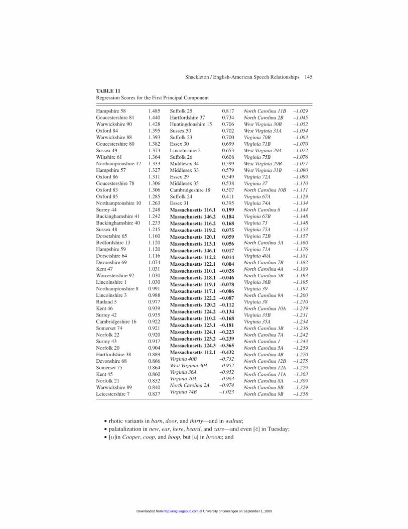
The factor scores for the first principal component, indicating the strength of thefeatures in informants’ speech, are shown in Table 11. Informants from the WestMidlands and Southwest of England have the highest positive scores, with nearlyall the lowest positive scores in England involving locales somewhat to the north-east of London. The principal component yields near-zero scores in Massachusetts,and negative scores in the American South—with eastern North Carolina localesgenerally earning the most negative scores. The first principal component, in sum,appears to distinguish a set of largely western English and often conservative fea-tures from largely eastern and typically innovative features. It also indicates thatthose eastern features are much more common in America than are the westernones; that is, all American dialects tend to be composed largely of variants that arefound mainly in southeastern England.
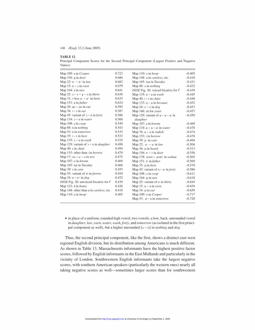
In contrast to the first, the second principal component, shown in Table 12, haslarge positive values for a group of variants that tend to be found in Massachusettsand in the southeast of England:
• nonrhotic variants in barn, door, thirty, and father;• an absence of palatalization in new, ear, here, chair, Tuesday, and care;
• [u] in Cooper, coop, and hoop, but [U] in broom; and• a fairly uniform, rounded and often relatively high backed vowel in daughter, law,
oxen, water, wash, forty, nothing, tomorrow, and dog.
The second principal component has large negative values for variants that tendto be found in the west of England and, fairly commonly, in the southern Americanregions:
144 JEngL 33.2 (June 2005)
TABLE 10Principal Component Scores for the First Principal Component (Largest Positive and Negative Values)
DSSE Fig. 16: other than œ before 0.807p, t, g, k, n, r
DSSE Fig. 32: h lost 0.782Map 106: a ~ A ~ c| in tomato 0.741DSSE Fig. 17 and PEAS Map 14: 0.741
other than œ before fricativesMap 51: variant of A in married 0.722Map 50: variant of E´ ~ e´ in Mary 0.694Map 26: centered onsets in nine 0.672DSSE Fig. 9: Middle English ou 0.651
not merged with Middle EnglishO · into an upgliding diphthong
Map 143: AI ~ c|I ~ åI in joint 0.650Map 171: s in greasy 0.643Map 133: A ~ a in because 0.624Map 129: variant of a ~ A ~ c| 0.616
in daughterMap 22: c| · in law 0.615Map 19: e´ ~ E´ in bracelet 0.612Map 169: v in nephew 0.600Map 125: U ~ Q in won’t 0.583Map 98: ai in neither or either 0.579Map 144: variant of oI etc. in boiled 0.579Map 43: u ~ U in four 0.565Map 75: a in hammer 0.564Maps 114, 115: U in soot 0.562Map 32: a· ~ a>· in father 0.560Map 131: a ~ A ~ c| in haunted 0.540Map 42: u ~ U in poor 0.537Map 45: variant of A ~ c| in forty 0.521DSSE Fig. 4: e´ ~ e· in three words 0.510
with eaMap 164: iu in new 0.506Maps 18-19: Middle English a· 0.504
distinct from Middle English ai
DSSE Fig. 4: other than e´ ~ e· in –0.510three words with ea
Maps 161-162: laibEri for library –0.519Map 45: variant of O ~ Å in forty –0.521Map 164: ju in new –0.531Map 40: œ in chair –0.535Map 143: Oi in joint –0.543Map 129: variant of O ~ Å in daughter –0.550Map 169: f in nephew –0.577Map 123: variant of o in home –0.611Map 171: z in greasy –0.631Maps 114, 115: U in soot –0.638Map 98: i in neither or either –0.644Map 144: Oi in boiled –0.645Map 131: œ in haunted –0.646Map 18: EI ~ eI in day –0.647DSSE Figs. 8 and 9: Middle English –0.651
ou merged with Middle EnglishO · into an upgliding diphthong
Maps 18-19: Middle English A· –0.655merged with Middle English ai
Map 51: œ in married –0.663Map 75: œ in hammer –0.674Maps 102-104: œ in parents –0.702Map 24: ÅO ~ OvO ~Oo in dog –0.716Map 19: EI ~ eI in bracelet –0.739DSSE Fig. 17 and PEAS Map 14: –0.741
œ before fricativesDSSE Fig. 32: h retained –0.782DSSE Fig. 16: œ before p, t, g, k, n, r –0.797Map 165: tjuz in Tuesday –0.812Map 106: variant of e in tomato –0.861
NOTE: PEAS = Pronunciation of English in the Atlantic States (Kurath and McDavid 1961); DSSE = Dialect Structureof Southern England (Kurath and Lowman 1970).
at University of Groningen on September 1, 2009 http://eng.sagepub.comDownloaded from
• rhotic variants in barn, door, and thirty—and in walnut;• palatalization in new, ear, here, beard, and care—and even [c&] in Tuesday;• [U]in Cooper, coop, and hoop, but [u] in broom; and
• in place of a uniform, rounded high vowel, two vowels: a low, back, unrounded vowelin daughter, law, oxen, water, wash, forty, and tomorrow (as isolated in the first princi-pal component as well), but a higher unrounded [U ~ U] in nothing and dog.
Thus, the second principal component, like the first, shows a distinct east-westregional English division, but its distribution among Americans is much different.As shown in Table 13, Massachusetts informants have the highest positive factorscores, followed by English informants in the East Midlands and particularly in thevicinity of London. Southwestern English informants take the largest negativescores, with southern American speakers (particularly the western ones) nearly alltaking negative scores as well—sometimes larger scores than for southwestern
146 JEngL 33.2 (June 2005)
TABLE 12Principal Component Scores for the Second Principal Component (Largest Positive and NegativeValues)
Map 109: u in Cooper 0.723Map 156: ´ê in door 0.686Map 22: Å · ~ Å·´ in law 0.682Map 15: Å ~ O in oxen 0.679Map 164: u in new 0.641Map 25: ‰ ~ Ä ~ V ~ U in thirty 0.638Map 31: r-less a· ~ A<· in barn 0.635Map 151: ´ in father 0.624Map 29: aU ~ AU in out 0.595Map 34: i ~ I in ear 0.587Map 45: variant of O ~ Å in forty 0.586Map 134: O ~ Å in water 0.560Map 108: u in coop 0.549Map 88: Å in nothing 0.543Map 53: Å in tomorrow 0.535Map 35: i ~ I in here 0.523Map 135: O ~ Å in wash 0.519Map 129: variant of O ~ Å in daughter 0.498Map 40: E in chair 0.494Map 153: other than i in borrow 0.478Map 17: Uu ~ u· ~ u in two 0.475Map 107: U in broom 0.469Map 165: tuz in Tuesday 0.466Map 39: E in care 0.455Map 55: variant of ‰r in furrow 0.454Map 24: Å ~ Å·´ in dog 0.452DSSE Fig. 30: unvoiced fricative for f 0.439Map 123: Q in home 0.426Map 148: other than ´ in careless, etc. 0.410Map 110: u in hoop 0.405
Map 110: U in hoop –0.405Map 148: ´ in careless, etc. –0.410Map 165: c&uz in Tuesday –0.431Map 88: U in nothing –0.432DSSE Fig. 30: voiced fricative for f –0.439Map 135: A ~ a in wash –0.445Map 40: i ~ I in chair –0.448Map 133: A ~ a in because –0.452Map 24: U ~ U in dog –0.453Map 166: ist for yeast –0.457Map 129: variant of a ~ A ~ c| in –0.459
daughterMap 107: u in broom –0.469Map 134: a ~ A ~ c| in water –0.470Map 76: a ~ A in radish –0.474Map 153: i in borrow –0.478Map 39: j‰ in care –0.494Map 22: c| · ~ A· in law –0.504Map 36: j‰ in beard –0.513Map 156: „ ~ r in door –0.558Map 178: OrnUt ~ OUnIt in walnut –0.565Map 151: „ in father –0.569Map 35: j‰ in here –0.570Map 45: variant of A ~ c| in forty –0.586Map 108: U in coop –0.611Map 164: ju in new –0.618Map 25: variant of „ in thirty –0.644Map 15: a ~ A in oxen –0.654Map 34: j‰ in ear –0.659Map 109: U in Cooper –0.717Map 53: c|~ A in tomorrow –0.720
at University of Groningen on September 1, 2009 http://eng.sagepub.comDownloaded from
English locales. The implications for American speech patterns are clear: the sec-ond principal component isolates a set of variants found primarily in both the Eng-
lish southwest and in the American south, and distinguishes them from a set ofvariants found in both the English southeast and in New England.
Principal components analysis of the data thus reveals two sets of oppositionswith fairly clear linguistic structural interpretations and distinct regional distribu-tions. As represented by Lowman’s informants, southern English speech has afairly strong demarcation between east and west. American speech forms appear todraw from all over the region (and possibly from others as well). However, Ameri-can forms tend to be similar to eastern English ones, on the whole, but northernAmerican forms tend to be much more so, while southern American speech revealssignificant western English affinities.12
The factor scores for both principal components are illustrated in Figure 7, thefirst on the vertical axis, the second on the horizontal. Note that the English infor-mants spread across the figure in a pattern roughly analogous to their geographicdistribution, while the American speakers form two distinct clusters, one in a dis-tinctly eastern position, the other, considered along the horizontal axis, positionedmidway between east and west.
Using Multiple Regression to Assessthe Importance of Geographic Distance
Multiple regression analysis, the workhorse of statistical analysis, refers to a setof statistical techniques that allow one to assess the relationship between a variableof interest—a dependent variable—and a number of other independent variables,allowing for interaction among the latter.13 For example, a researcher may use mul-
tiple regression to analyze how individuals’weight is simultaneously influenced bytheir height, waistline, and age.
Regression analysis can be used to test for a relationship between American in-formants’degrees of similarity with English informants and the latters’geographiclocation. For instance, it may reveal a tendency for American informants to havemore variants in common with English informants from nearest the metropolitanarea and thus may lend support to the proposition that one cause of the relative uni-formity of American speech, as well as its relative similarity to southeastern variet-ies of English, is the fact that many immigrants came from near London. Accordingto Bailyn (1986), London was absorbing more or less all of the natural increase inpopulation in Britain during at least part of the period of American colonization,and many migrants to America did so after first coming to London. It is important tonote, however, that they migrated to London, not to the rural areas in the vicinity ofLondon. As mentioned previously, English informants living only a few scoremiles from London tend to cluster rather regularly into separate, distinct clustersrather than into a London-centered one, suggesting that population movements toLondon had relatively little effect on the speech patterns of rural speakers in thesurrounding region.
Table 14 shows the results of a series of twelve regressions. In each regression,the values for one of the measures of similarity between all the informants from oneof the American regions and all English informants are regressed against the dis-tances in miles of the English informants’ localities from London. The parameterlabeled “distance” provides an estimate of how much an increase in an English in-formant’s distance from London affects the informant’s similarity with informantsfrom the American region.
In the top left-hand regression, for example, the constant term indicates that ac-cording to the correlations in the data set, a hypothetical informant living in Londonwould share about 42.6 percent of his or her variants with a typical Massachusettsinformant. The parameter for the distance variable indicates that one hundred milesof distance from London reduces an English speaker’s proportion of shared vari-ants with a typical Massachusetts speaker by about 6 percentage points. (The valueof the parameter, –0.0006, times 100, yields –0.06, or minus 6 percentage points.)The low value of the “significance” measure paradoxically indicates that the valueof the parameter is relatively well constrained and the estimate is relativelyaccurate. The adjusted R-squared indicates that the regression accounts about foronly about 7 percent of the variance in the percentage of variants shared betweenMassachusetts and southern English informants. The standard error indicates thatusing this equation, the typical estimate of a Massachusetts informant’s sharedvariants with an English informant will be off by nearly 8 percentage points.
Another regression directly below the first includes another set of variables;these are regional “dummy” variables that take a value of 1 if the English informant
is in a given region and 0 otherwise. That regression allows us to gauge the impor-tance of distance from London while allowing for the fact that American infor-mants may have different degrees of similarity with English informants from dif-ferent regions. When dummy variables are used for a set of groups in a regression,one group is excluded, and the constant that is estimated in the regression is inter-preted as the dummy for that group. In this case, the Southeast is excluded, and theconstant term in the equation provides an estimate of the average degree of similar-ity between informants from the American region and a hypothetical Southeasternspeaker living on the southern edge of London.
The second regression indicates that using the shared variants measure, all elsebeing equal, the typical Massachusetts informant shares nearly 46 percent of his orher variants with that hypothetical Southeastern English speaker. The parameter forthe distance variable takes a much smaller value than in the previous regression,and now indicates that one hundred miles of distance from London reduces an Eng-lish speaker’s proportion of shared variants with a typical Massachusetts speakerby about 2 percentage points, all else being equal, strongly suggesting that much ofthe variation accounted for by the distance parameter alone in the previous regres-sion may be more appropriately accounted for by regional affiliation. Informantsfrom East Anglia, the Southwest, and Devonshire will typically share significantlylower percentages of variants with Massachusetts informants than the English in-
formants’distance from London alone would dictate—about 4.4, 12.5, and 5.2 per-centage points lower, respectively. The significance values of practically zero indi-cate that those parameter estimates are well constrained. In contrast, the parametersfor the East Midlands and West Midlands dummy variables—which indicate thatinformants from those regions will typically share about two-thirds of a percentagepoint fewer variants with an informant from Massachusetts than a Southeastern in-formant living equidistant from London—are not significant, indicating that it isdifficult to distinguish between the importance of distance for the Southeastern in-formants and those from the Midlands regions. In effect, distances to the west mat-ter a great deal more than distances to the north and east, and the inclusion of re-gional variables brings that difference out of the data. The adjusted R-squaredindicates that distance and regional dummy variables account about for more thanhalf of the variance in the percentage of variants shared between Massachusetts andsouthern English informants, with regional variations rather than distance fromLondon accounting for most of that difference.
The shared variants regressions for southern American informants generallyfollow the same pattern. Regional location appears to be more important than dis-tance from London in determining whether English informants have greater affin-ity with American ones. The regression for Eastern Virginians also yields a smallbut significant negative distance parameter estimate, again suggesting that Ameri-can speakers do indeed have slightly greater similarity with rural speakers fromnear London. The parameter is much smaller, however, if regional variables are in-cluded in the regression, again suggesting that much of the variation accounted forby the distance parameter alone in the previous regression may be more appropri-ately accounted for by regional affiliation. The regression for Western Virginians,however, yields a zero distance parameter without regional dummies and a positivebut insignificant one without it, indicating that distance from London has no inde-pendent affect on the similarity between English informants and American infor-mants from that region. The negative parameters for all but one of the regional vari-ables for the regressions that include such variables indicate that southernAmericans typically share significantly fewer variants with informants in other re-gions than they do with informants from the Southeast (except, insignificantly, forWestern Virginians compared to informants from Devonshire). Note that values ofthe Eastern and Western Virginians’ regional parameters are rather similar to eachother, compared with those of the New Englanders, and that the American south-erners’ regional parameters are more negative for the Midlands regions and lessnegative for the other regions than is the case for the New Englanders. Note also thatthe regressions for the American southerners have lower adjusted R-squares, indi-cating that regional affiliation and distance from London together account for lessof the variation in their affinities with English informants, but that the regressionshave lower standard errors than the ones for New Englanders, due to the relatively
152 JEngL 33.2 (June 2005)
at University of Groningen on September 1, 2009 http://eng.sagepub.comDownloaded from
uniform character of their speech patterns. The results are entirely consistent withearlier findings: the American southerners show greater affinity with westernspeakers and less affinity with eastern speakers than do Massachusetts speakers,but their affinities are more diffuse altogether even though their speech isremarkably uniform.
The regressions on the linguistic distance measure yield essentially the same re-sults, although the signs of the parameters are reversed because large values forthese measures indicate lesser rather than greater similarity. The addition of re-gional parameters affects the distance parameter estimate in a similar way; the re-gional parameters and their significances vary across English regions in a similarway; and the adjusted R-squares vary across American regions in a similar way. Theregressions are generally all consistent with the proposition that American speechforms tend to be most similar to those immediately surrounding London and(mildly) progressively less similar in more distant regions, with the relation appar-ently stronger for Massachusetts speakers than for southern speakers. However, theregional affiliation of English informants is consistently more important inaccounting for affinities with American informants than is distance from themetropolis.
Conclusions
In summary, the application of a variety of quantitative techniques to patterns ofusage by twentieth-century English and American informants appears to provideseveral insights into the nature of southern English and American speech. Theanalysis reveals a tremendous amount of diversity among southern English infor-mants, distinguishes six more or less distinct southern English dialect regions, sim-ilar in geographic distribution to regions delineated in previous studies, and showsthat the variants found among American informants were nearly all found among atleast some informants in southern England. That finding appears to indicate wide-spread preservation of English variants and relatively little phonetic innovation inAmerica—at least in the sense of creation of entirely distinct phonemes. As gaugedby several different measures, the American varieties of English analyzed here ap-pear to be quite comfortably placed in the family of southern English dialects, atleast in terms of their phonetic characteristics, and American varieties appear to dif-fer from their English counterparts primarily in composition. At the same time, theoverall diversity within and among American regions is considerably less than thatwithin and among the English regions, suggesting extensive—but different—leveling processes and the extinction of many—but different—English variants ineach American region.
Variants found in American regions are typically more likely to be found in thesoutheastern regions of England and particularly in the southeast closest to Lon-
don. The similarity has structural elements, including important phonetic mergers,raising of low front vowels, and retraction and rounding of back ones. However, theanalysis also reveals different leveling processes in different American regions:variants found in Massachusetts, taken as a whole, tend to be considerably differentfrom those observed in the two southern American regions, while the southern re-gions tend to be much more similar to each other in usage. Informants from Massa-chusetts consistently show substantially greater similarity with East Midlands in-formants than with those of southwestern England. In contrast, variants commonamong southern American informants but not found in Massachusetts often appearto be more similar to those found in southwestern England—these similarities alldespite the passage of centuries since the earliest colonization, and consistent withCleanth Brooks’s (1935, 73) observation more than sixty years ago that southernAmerican English was “strongly colored” by that of southwestern England. Thesecondary influence of the East Midlands on Massachusetts and of the EnglishSouthwest on the American south also involves identifiable structural elements,with rhoticity, palatalization, and certain shifts in back vowels present in the latterregions and absent in the former ones.
American phonetic speech patterns thus appear to be largely amalgams of south-ern English variants, with a dominant influence from the regions closest to the capi-tal but with significant East Midlands influence in the New England and greatersouthwestern influence in Virginia. Except for the absence of clear East Anglian in-fluence on the speech of Massachusetts, the results are largely consistent with thehistorical record of the regional migrations from seventeenth- and eighteenth-century Britain to North America, which suggests that the Puritan migration toMassachusetts drew largely from the eastern counties of England, while the migra-tion to the Tidewater region drew mainly from the metropolitan center aroundLondon and from the southwest.
The relative uniformity of American speech may stem in part from the domi-nance of immigrants from southeastern England. Perhaps a third of the British im-migrants to America came from near London, while other regions tended to con-tribute smaller shares to the total immigration. Of the 155,000 English immigrantswho settled in the mainland North American colonies in the seventeenth century,most were indentured servants who sailed from London and came from the Thamesvalley. Despite changes in the regional patterns of emigration during the eighteenthcentury, the bulk of English settlers continued to come from the southeast.14 Itseems very likely that those migrants formed a large enough portion of the early im-migrant population that their speech forms tended to dominate in the developmentof distinctive American colonial varieties, contributing to the leveling process. As aresult, metropolitan (or near-metropolitan) variants would likely have been spokenby a large share of the early settlers, or possibly accorded somewhat greaterprestige, or both.
154 JEngL 33.2 (June 2005)
at University of Groningen on September 1, 2009 http://eng.sagepub.comDownloaded from
It is important to take into account the fact that during the period of colonization,internal migration was bringing an enormous number of people from all over Brit-ain to London, and that that process could reasonably be expected to have influ-enced rural speech in the region of London. Similarities between American andSoutheastern English speech may therefore simply indicate that a process parallelto the leveling that occurred in the colonies also occurred in the Southeast, resultingin relatively large similarities between those regions. As noted previously, how-ever, informants from rather near London do not tend to cluster into a distinctivemetropolitan group, or even to cluster strongly with a single region. Rather, theyseem to have stronger affinities with regions not clearly related to London at all thanthey do with each other. To be sure, Southeastern informants tend to show some-what greater affinity with those from the East Midlands, but that comparative simi-larity of East Midlands and Southeastern speech is of very long standing and isthought to be related to population movements preceding the early modern era.15 Ittherefore seems unlikely that the relatively high degree of similarity betweenAmerican speech and that of the English Southeast is due primarily to leveling inthe vicinity of London.16
Those conclusions may help explain why eighteenth-century English visitorsnoticed little variation in American regional speech forms. If they were familiarwith southeastern English rural speech, American speech probably struck them notonly as similar but as similar in its variation. It would also explain why, as Londonspeech and an English standard each became increasingly distinct from the sur-rounding, increasingly less prestigious rural dialects, and as American speechforms evolved independently, nineteenth-century English visitors to Americawould note both the uniformity of American speech and the difference betweenAmerican speech and proper English, but would not necessarily note a distinctsimilarity of American speech to any particular English dialect.
Because the patterns of variation involve increasing numbers of variants in re-gions with more informants and with longer-settled populations as well as high di-versity in the home country coupled with extensive but varying patterns of levelingin the colonies, they are reminiscent of the species-age-area relationships found inpopulation biology and the effects of evolutionary bottlenecks found in the analysisof population genetics. A process of leveling—analogous to the loss of species dur-ing reduction in habitat—appears to have reduced the population of variants duringthe colonial settlement of North America, leaving American speech patterns rela-tively uniform, though with differences that may be traced back to differences in thefounding populations. Thus, the similarity between eastern and western Virginiaspeech forms suggests that the dominant influence on the development of speechpatterns in the American south came from the regions of earliest settlement, provid-ing support for Mufwene’s (1996) Founder Principle. On the whole, the results areconsistent with Mufwene’s model of competition and selection of linguistic fea-
tures, in which “units and principles selected from different varieties . . . arerestructured into a new system.” They are also consistent with Kretzschmar’s(2002) contention that
linguistic features were retained from the habits of individual speakers, butnot whole linguistic systems from constituent immigrant languages or dia-lects. The default condition for English in the colonies in the seventeenth cen-turies was no “London standard” (whatever that could have meant given thegreat population mobility of the time), but instead a pool of linguistic featurescollected from a radically mixed settlement population. (237)17
A largely southeastern English origin for American speech is also consistentwith the recognition of a largely southeastern English origin for other forms of co-lonial English. On the basis of the present analysis, it seems very likely that pro-cesses quite similar to those that produced new varieties of English in Australia andNew Zealand in the nineteenth century produced American English forms duringthe seventeenth and early eighteenth.
Notes
1. For a relatively Anglocentric view, see Wolfram and Schilling-Estes (1998,93). For a quite contrary view, see Dillard (1992, 1-31).
2. Heeringa (2004) provided a very useful summary of much of that research.3. The descriptions of English informants are taken from Viereck (1975); of
Massachusetts informants, from Kurath (1939); and of southern American infor-mants, from Kretzschmar et al. (1994).
4. There are many clustering procedures, some of which involve the use of sta-tistical probabilities or statistical measures, but in general the procedures are notproperly thought of as statistical since most do not assess the probability that obser-vations are “correctly” classified. See Romesburg (2004) for a detailed discussionof cluster analysis.
5. In principle, clustering techniques can incorporate any distance measure onewishes, with some measures being more appropriate for some types of data than forothers. For this analysis, a measure of linguistic distance would likely be most ap-propriate. That, however, is a direction for future work; for simplicity the analysisrelies instead on a few measures typically available in a standard package: Euclid-ean distances, Pearson correlations, and cosines.
6. Unfortunately, Lowman does not appear to have interviewed any Cockneys.An informant who had acquired working-class London speech in the mid- to late-nineteenth century would have been an invaluable addition to the survey.
156 JEngL 33.2 (June 2005)
at University of Groningen on September 1, 2009 http://eng.sagepub.comDownloaded from
7. See Heeringa (2004), especially chapter 3, for a highly detailed discussion ofsuch approaches to measuring linguistic distance. The approach used in this study ismost similar to that of Almeida and Braun (1985), discussed in Heeringa (pp. 40-45).
8. Another set of distance measures are available from genetic research, whichdeals with problems that are in many ways analogous to those of historical linguis-tics and dialectology. Measures of genetic distance are typically based on therelative frequencies of different genetic variants or alleles of a given gene. Suchmeasures can be applied to linguistic data, treating variants of a given phoneme asanalogous with alleles of a given gene. One such measure, Nei’s genetic distance(D), measures how closely related populations are under the assumption thatchange is always to a completely new variant, all genes have the same rate ofchange, and the populations remain constant in size over time. Exactly similar pat-terns of variants will yield a value of 0.00; two informants with 50 percent sharedvariants will yield a value of roughly 0.7; two informants with one shared variantwill yield a value of about 4.4, and two entirely dissimilar informants yield an infi-nite value. Measuring D in the sample used in this study yield values ranging from0.00 to 1.70. An analysis of Nei’s distances among informants yields essentially ex-actly the same insights as obtained from the analysis of shared variants. The qualityof the data apparently does not allow the greater sophistication of the technique toyield any more insight than can be gained from a more transparent measure. More-over, the data characteristics that make Nei’s distance most appropriate do not ob-tain in the case of language change: linguistic change need not involve shifts to en-tirely new variants or uniform rates of change; and the populations of speakers havecertainly not remained constant over time.
9. See Tabachnick and Fidell (2000) for a useful overview of principal compo-nents and factor analysis.
10. Technically, standard principal components analysis extracts maximumvariance from a data set using orthogonal vectors projected through the data: eachsuccessive component minimizes the sum of squared deviations remaining after theprevious one, subject to the constraint that the component be orthogonal to the pre-vious one(s). Variants on standard principal component analysis that “rotate” thePCs allow for a trade-off between orthogonality of components and extraction ofvariance.
11. The analysis is discussed in Labov, Ash, and Boberg (forthcoming), chapter11, pp. 79-85, which can be accessed at http://www.ling.upenn.edu/phono_atlas/Atlas_chapters/Ch11.pdf.
12. The shortening of different words of the coop/hoop/broom family appearsparticularly diagnostic of English-American relations. Map 18 in Anderson (1987,36) documents the widespread tendency to shorten similar words throughoutsouthern England, particularly in a belt from East Anglia to the West Midlands.
However, different words tend to be shortened in different regions of southern Eng-land, and so it seems particularly interesting that the pattern of shortening variesacross New England and the American South much as it varies from the southeastof England to the southwest.
13. See Tabachnick and Fidell (2000) for a useful overview of multiple regres-sion analysis.
14. For extensive discussion of seventeenth- and eighteenth-century immigra-tion patterns, see Bailyn (1986) and Fischer (1989).
15. Anderson (1987, 3) argued that the “evidence points to a transfer of popula-tion from the central Midlands to the South East such as is known to have occurredin the medieval period.”
16. Despite the massive internal migrations, London itself was still a fairly smallcity in the seventeenth century, mainly because extremely high mortality rateslargely kept pace with the rate of migration.
17. See Mufwene (2002) and Kretszchmar (2002).
References
Algeo, John. 2003. The Origins of Southern American English. In English in theSouthern United States, ed. Stephen J. Nagle and Sara L. Sanders, 6-16. Cam-bridge: Cambridge University Press.
Almeida, A., and A. Braun. 1985. “Richtig” und “Falsch” in phonetischerTranskription; Vorschläge zum Vergleich von Transkriptionen mit Beispielenaus deutschen Dialekten. Zeitschrift für Dialektologie und Linguistik 53 (2):158-72.
Anderson, Peter M. 1987. A Structural Atlas of the English Dialects. London:Croom Helm Ltd.
Bailey, Guy. 1997. When Did Southern American English Begin? In Englishesaround the World, vol. 1, General Studies, British Isles, North America, ed. Ed-gar W. Schneider, 255-75. Philadelphia: John Benjamins Publishing Company.
Bailyn, Bernard. 1986. The Peopling of British North America: An Introduction.New York: Random House.
Brooks, Cleanth. 1935. Relation of the Alabama-Georgia Dialect to the ProvincialDialects of Great Britain. Baton Rouge: Louisiana State University Press.
Carver, Craig M. 1987. American Regional Dialects: A Word Geography. Ann Ar-bor: University of Michigan Press.
Dillard, J. L. 1992. A History of American English. New York: Longman.Fischer, David Hackett. 1989. Albion’s Seed: Four British Folkways in America.
New York: Oxford University Press.Heeringa, Wilbert. 2004. Measuring Dialect Pronunciation Differences Using
Levenshtein Distance. Groningen Dissertations in Linguistics 46. Groningen,the Netherlands: Author.
158 JEngL 33.2 (June 2005)
at University of Groningen on September 1, 2009 http://eng.sagepub.comDownloaded from
Kretzschmar, William A. 2002. “American English: Melting Pot or Mixing Bowl?”in Of Dyuersitie & Chaunge of Langage: Essays presented to Manfred Görlach,ed. K. Lenz and R. Möhlig, 224-39. Heidelberg, Germany: C. Winter.
Kretzschmar, William A., Virginia G. McDavid, Theodore K. Lerud, and EllenJohnson. 1994. Handbook of the Linguistic Atlas of the Middle and South Atlan-tic States. Chicago: University of Chicago Press.
Kretzschmar, William A., and Susan Tamasi. 2002. Distributional Foundations fora Theory of Language Change. World Englishes 22 (4): 377-401.
Kurath, Hans, ed. 1939. Linguistic Atlas of New England. Providence, RI: BrownUniversity.
Kurath, Hans, and Guy Lowman Jr. 1970. The Dialect Structure of Southern Eng-land: Phonological Evidence. Publications of the American Dialect Society no.54. Tuscaloosa: University of Alabama Press.
Kurath, Hans, and Raven I. McDavid Jr. 1961. The Pronunciation of English in theAtlantic States. Ann Arbor: University of Michigan Press.
Labov, William, Sharon Ash, and Charles Boberg. Forthcoming. Atlas of NorthAmerican English. New York: DeGruyter.
Montgomery, Michael B. 2001. British and Irish Antecedents. In Cambridge His-tory of the English Language, vol. 6, English in North America, ed. John Algeo86-153. Cambridge: Cambridge University Press.
Mufwene, Salikoko. 1996. The Founder Principle in Creole Genesis. Diachronica13 (1): 83-134.
. 2002. Competition and Selection in Language Evolution. Selection 3 1:45-56.Nerbonne, John. 2005. Various Variation Aggregates in the LAMSAS South.
Schneider, Edgar W. 2003. Shakespeare in the Coves and Hollows? Toward a His-tory of Southern English. In English in the Southern United States, ed. StephenJ. Nagle and Sara L. Sanders, 17-35. Cambridge: Cambridge University Press.
Tabachnick, Barbara G., and Linda S. Fidell. 2000. Using Multivariate Statistics.Boston: Allyn & Bacon.
Trudgill, Peter. 1986. Dialects in Contact. Oxford, UK: Blackwell.. 1990. The Dialects of England. Oxford, UK: Blackwell.. 2004. New-Dialect Formation: The Inevitability of Colonial Englishes.
Oxford: Oxford University Press.Viereck, Wolfgang. 1975. Lexicalische und grammatische Ergebnisse des
Lowman-Survey von Mittl- und Südengland. München, Germany: WilhelmFink Verlag.
Wright, Laura. 2003. Eight Grammatical Features of Southern United StatesSpeech Present in Early Modern London Prison Narratives. In English in theSouthern United States, ed. Stephen J. Nagle and Sara L. Sanders, 36-63. Cam-bridge: Cambridge University Press.
Robert G. Shackleton Jr. is a principal analyst in the Macroeconomic Analy-sis Division of the Congressional Budget Office in Washington, D.C. Hisprincipal areas of research are the economics of climate change, the interna-tional macroeconomic implications of the global demographic transition,and retirement preparations among Baby Boomers. His area of interest inlinguistic research is the origin and diffusion of American dialect features.
160 JEngL 33.2 (June 2005)
at University of Groningen on September 1, 2009 http://eng.sagepub.comDownloaded from