Journal of Hydrology 401 (2011) 190–202

Contents lists available at ScienceDirect

Journal of Hydrology

journal homepage: www.elsevier .com/locate / jhydrol

Uncertainty of downscaling method in quantifying the impact of climate changeon hydrology

Jie Chen ⇑, François P. Brissette, Robert LeconteDepartment of Construction Engineering, École de Technologie Supérieure, Université du Québec, 1100 Notre-Dame Street West, Montreal, QC, Canada H3C 1K3

a r t i c l e i n f o

Article history:Received 28 July 2010Received in revised form 12 February 2011Accepted 16 February 2011Available online 22 February 2011

This manuscript was handled byA. Bardossy, Editor-in-Chief, with theassistance of Martin Beniston, AssociateEditor

Keywords:Climate changeUncertaintyDownscalingHydrologyPrecipitationTemperature

0022-1694/$ - see front matter � 2011 Elsevier B.V. Adoi:10.1016/j.jhydrol.2011.02.020

⇑ Corresponding author. Tel.: +1 514 396 8800.E-mail address: chj092413@yahoo.com.cn (J. Chen

s u m m a r y

Uncertainty estimation of climate change impacts has been given a lot of attention in the recent litera-ture. It is generally assumed that the major sources of uncertainty are linked to General Circulation Mod-els (GCMs) and Greenhouse Gases Emissions Scenarios (GGES). However, other sources of uncertaintysuch as the choice of a downscaling method have been given less attention. This paper focuses on thisissue by comparing six downscaling methods to investigate the uncertainties in quantifying the impactsof climate change on the hydrology of a Canadian (Quebec province) river basin. The downscaling meth-ods regroup dynamical and statistical approaches, including the change factor method and a weathergenerator-based approach. Future (2070–2099, 2085 horizon) hydrological regimes simulated with ahydrological model are compared to the reference period (1970–1999) using the average hydrograph,annual mean discharge, peak discharge and time to peak discharge as criteria. The results show thatall downscaling methods suggest temperature increases over the basin for the 2085 horizon. The regres-sion-based statistical methods predict a larger increase in autumn and winter temperatures. Predictedchanges in precipitation are not as unequivocal as those of temperatures, they vary depending on thedownscaling methods and seasons. There is a general increase in winter discharge (November–April)while decreases in summer discharge are predicted by most methods. Consistently with the large pre-dicted increases in autumn and winter temperature, regression-based statistical methods show severeincreases in winter flows and considerable reductions in peak discharge. Across all variables, a largeuncertainty envelope was found to be associated with the choice of a downscaling method. This envelopewas compared to the envelope originating from the choice of 28 climate change projections from a com-bination of seven GCMs and three GGES. Both uncertainty envelopes were similar, although the latter wasslightly larger. The regression-based statistical downscaling methods contributed significantly to theuncertainty envelope. Overall, results indicate that climate change impact studies based on only onedownscaling method should be interpreted with caution.

� 2011 Elsevier B.V. All rights reserved.

1. Introduction major obstacle (Leavesley, 1994; Hostetler, 1994; Xu, 1999). It is

The Intergovernmental Panel on Climate Change (IPCC, 2007)stated that there is high confidence that recent climate changeshave had discernible impacts on physical and biological systems.Many General Circulation Models (GCMs) consistently predict in-creases in frequency and magnitudes of extreme climate eventand variability of precipitation (IPCC, 2007). This will affect terres-trial water resource in the future, perhaps severely (Srikanthan andMcMahon, 2001; Xu and Singh, 2004). For continental water re-sources, hydrological models are frequently used to quantify thehydrological impacts of climate change using GCM data as inputs(Salathe, 2003; Diaz-Nieto and Wilby, 2005; Minville et al., 2008,2009). However, the spatial resolution mismatch between GCMsoutputs and the data requirements of hydrological models is a

ll rights reserved.

).

therefore necessary to perform some post-processing to improveupon these global-scale models for impact studies. Consequently,dynamical downscaling (regional climate models, RCMs) and sta-tistical downscaling (SD) methods have been developed to meetthis requirement. RCMs are developed based on dynamic formula-tions using initial and time-dependent lateral boundary conditionsof GCMs to achieve a higher spatial resolution at the expense oflimited area modeling (Caya and Laprise, 1999). The main problemof RCMs is the computational cost (Solman and Nunez, 1999). Thus,it is only available for limited regions. Moreover, despite improve-ments, outputs of RCMs are still too coarse for some practicalapplications, like small watershed hydrological and field agricul-tural impact studies, which may need local and site-specific cli-mate scenarios. SD techniques have been developed to overcomethese challenges. They involve linking the state of some variablesrepresenting a large scale (GCM or RCM grid scale, the predictors)and the state of other variables representing a much smaller scale

J. Chen et al. / Journal of Hydrology 401 (2011) 190–202 191

(catchment or site scale, the predictands). These techniques arecomputationally cheap and relatively easy to implement.

These SD techniques fall into three categories: transfer function(Wilby et al., 1998, 2002), weather typing (von Stoch et al., 1993;Schoof and Pryor, 2001) and weather generator (WG) (Wilks, 1999;Zhang, 2005). Transfer function approaches involve establishingstatistical linear or nonlinear relationships between observed localclimatic variables (predictands) and large-scale GCM outputs (pre-dictors) (Wilby et al., 2002). They are relatively easy to apply, buttheir main drawback is the probable lack of a stable relationshipbetween predictors and predictands (Wilby and Wigley, 1997).Weather typing scheme involves grouping local meteorologicalvariables in relation to different classes of atmospheric circulation(Bardossy and Plate, 1992; von Stoch et al., 1993). The main advan-tage is that local variables are closely linked to global circulation.However, its reliability depends on a stationary relationship be-tween large-scale circulation and local climate. Especially for pre-cipitation, there is frequently no strong correlation between dailyprecipitation and large-scale circulation. The WG method is basedon the perturbation of its parameters according to the changes pro-jected by climate models (Zhang, 2005; Kilsby et al., 2007; Qianet al., 2005, 2010; Wilks, 2010). The appealing property is its abilityto rapidly produce sets of climate scenarios for studying the im-pacts of rare climate events and investigating natural variability.

Another relatively straightforward and popular downscalingmethod for rapid impact assessment of climate change is thechange factor (CF) method (Minville et al., 2008; Diaz-Nieto andWilby, 2005; Hay et al., 2000). It involves adjusting the observedtime series by adding the difference (for temperatures) or multi-plying the ratio (for precipitation) between future and present cli-mates as simulated by the RCMs or GCMs. The most significantdrawbacks are that the temporal sequencing of wet and dry days,and that the variances of temperatures are unchanged.

The unique advantages and drawbacks of each downscalingmethod result in different future climate projections. In particular,some downscaling methods are unable to capture the extremes ofclimate events that are often of particular concern in hydrology.Differences in future climate projections imply that downscalingmethods add uncertainties in quantifying the impacts of climatechange on hydrology. Many studies have focused on uncertaintieslinked to GCMs (Graham et al., 2007a,b; Maurer and Hidalgo, 2008;Minville et al., 2008; Christensen and Lettenmaier, 2007; Hamletand Lettenmaier, 1999). Rowell (2006) compared the effect of dif-ferent sources of uncertainty including emissions scenario, GCM,RCM and initial condition ensembles on changes in seasonal pre-cipitation and temperature for the UK. The uncertainty from aGCM was found to be the largest. Prudhomme and Davies (2009)used three GCMs, two greenhouse gas emission scenarios (GGES)and two downscaling techniques (statistical downscaling model(SDSM) and HadRM3) to investigate their uncertainty in propagat-ing river flow, and demonstrated that uncertainties from GCMs arelarger than those from downscaling methods and GGES. Kay et al.(2009) also investigated different sources of uncertainties includ-ing GGES, GCM’s structure (five GCMs), downscaling method (CFand RCM), hydrological model structure (two models), hydrologi-cal model parameters (jack-knifed calibrated parameter sets) andthe internal variability of the climate system on the impact of cli-mate change on flood frequency in England. With this research,each different source of uncertainty was done individually ratherthan in combination with each other. The results showed thatthe uncertainty related to GCM structure is the largest, but thatother sources of uncertainty are significant if the GCM structure’sinfluence was not taken into account. Wilby and Harris (2006) pre-sented a probabilistic framework for quantifying different sourcesof uncertainties on future low flow. They used four GCMs, twoGGES, two downscaling techniques (SDSM and CF), two hydrolog-

ical model structures and two sets of hydrological model parame-ters. The results indicated that GCMs revealed the greatestuncertainty, followed by downscaling methods. Uncertainties dueto hydrological model parameters and GGES were less important.

Generally, GCMs are considered to be the largest source ofuncertainty for quantifying the impacts of climate change.However, the uncertainty related to the downscaling and bias-correction methods must be taken into account for better estima-tion of the impact of climate change (Quintana Segui et al, 2010).Moreover, although some studies attempted to investigate theuncertainty related to downscaling techniques, only two methodswere involved. A better method may use multi-downscalingtechniques (more than two) for quantifying their uncertaintypropagation in hydrology.

The objective of this study is to quantify the impacts of climatechange on a Canadian river basin (Quebec province), while investi-gating the uncertainties related to downscaling techniques, usingsix downscaling methods. The downscaling methods include bothdynamical and statistical approaches, including the CF methodand a WG-based approach.

2. Study area and data

2.1. Study area

This study was conducted for the Manicouagan 5 river basin lo-cated in central Quebec, Canada. It covers 24,610 km2 of mostlyforested areas (Fig. 1). It has a rolling to moderately hilly topogra-phy with a maximum elevation of 952 m above sea level. The res-ervoir at the basin outlet has a mean level of 350 m above sea level.Population density is extremely low and logging is the only indus-trial activity over the basin. The basin drains into the Manicouagan5 reservoir, a 2000 km2 annular reservoir within an ancient erodedimpact crater. The basin ends at the Daniel Johnson dam which isthe largest buttressed multiple arch dam in the world. The in-stalled capacity of the dam is 2.6GW. The annual mean dischargeof the Manicouagan 5 River is 529 m3/s. Snowmelt peak dischargeusually occurs in May and averages 2200 m3/s.

2.2. Data

The different datasets used in this work are summarized inTable 1. Observed data consisted of precipitation, maximum tem-perature (Tmax) and minimum temperature (Tmin) interpolatedon a 10 km grid by the National Land and Water InformationService (www.agr.gc.ca/nlwis-snite). The interpolation is per-formed using a thin plate smoothing spline surface fitting method(Hutchinson et al., 2009). Discharge data at the basin outlet wasobtained from mass balance calculations at the dam and were pro-vided by Hydro-Québec. Climate data consisted of reanalysis, GCMand RCM data. Data from the Canadian GCM (v3.1) (CGCM) and theCanadian RCM (v.4.2.0) (CRCM) was used. Average grid resolutionwas about 300 km for the CGCM and 45 km for the CRCM. The Na-tional Center for Environmental Prediction (NCEP) reanalysis datawas used as a proxy to GCM data, to calibrate some of the down-scaling used in this paper. This data uses a T62 (�209 km) globalspectral model to consistently collect observational data from awide variety of observed sources (Kalnay et al., 1996; DAI CGCM3Predictors, 2008). It includes information from both models andobservations. SD techniques were calibrated using NCEP predictorsinterpolated at the CGCM scale. In climate change mode, predictorsfrom the CGCM were used directly. The CRCM data driven by NCEPwas also used for calibration purposes, while in climate changemode it was driven by the CGCM at its boundary and initial condi-tions. This work covers the 1970–1999 period (reference period)

Fig. 1. Location map of Manicouagan 5 river basin.

Table 1The datasets used in this research.

No. Dataset Purpose Time period

1 Observed P, Tmax and Tmin (interpolated at a 10 kmscale – NLWIS dataset), measured discharge

Baseline, calibration of Hydrological model and WG 1970–1999

2 CGCM P, Tmax and Tmin Downscaling of CF and WG methods 1970–1999, 2070–20993 CRCM P, Tmax and Tmin Downscaling of CF and WG, and CRCM

with and without BC methods1970–1999, 2070–2099

4 NCEP predictors interpolated to CGCM grid Calibration of SDSM and DASR 1970–19995 CGCM predictors Downscaling of SDSM and DASR 2070–20996 CRCM P, Tmax and Tmin driven by NCEP Calibration of HM for the method of

CRCM without BC1970–1999

Note: P = precipitation; Tmax = maximum temperature; Tmin = minimum temperature; BC = bias correction; WG = weather generator; SDSM = statistical downscalingmodel, and DASR = discriminant analysis coupled with stepwise linear regression downscaling method.

Table 2NCEP and CGCM predictor variables used to select precipitation predictors for downscaling.

Predictor variable Abbreviation Predictor variable Abbreviation

Mean sea level pressure ncepmslp 500 hPa Divergence ncepp5zh1000 hPa Wind Speed ncepp_f 850 hPa Wind Speed ncepp8_f1000 hPa U-component ncepp__u 850 hPa U-component ncepp8_u1000 hPa V-component ncepp__v 850 hPa V-component ncepp8_v1000 hPa Vorticity ncepp__z 850 hPa Vorticity ncepp8_z1000 hPa Wind Direction ncepp_th 850 hPa Geopotential ncepp8501000 hPa Divergence ncepp_zh 850 hPa Wind Direction ncepp8th500 hPa Wind Speed ncepp5_f 850 hPa Divergence ncepp8zh500 hPa U-component ncepp5_u 500 hPa Specific Humidity ncep s500500 hPa V-component ncepp5_v 850 hPa Specific Humidity nceps850500 hPa Vorticity ncepp5_z 1000 hPa Specific Humidity ncepshum500 hPa Geopotential ncepp500 Temperature at 2 m nceptemp500 hPa Wind Direction ncepp5th

192 J. Chen et al. / Journal of Hydrology 401 (2011) 190–202

for calibration and the 2070–2099 period (2085 horizon) in climatechange mode. The atmospheric predictors considered (NCEP andCGCM) are listed in Table 2.

3. Methodology

3.1. Downscaling methods

Six downscaling methods will be compared in this work.They consist of using CRCM data with (1) and without (2) bias

correction, CF (3) and WG (4) methods at both CGCM and CRCMscales and two statistical downscaling methods: SDSM (5) and dis-criminant analysis coupled with step-wise regression method (6)at CGCM scale. Table 3 briefly describes all of the methods. Detailsfollow below.

3.1.1. Canadian RCM without bias correctionWith the improved resolution of RCMs and the relatively small

biases of RCM output data (compared to GCM data), it is now pos-sible to envision direct use of RCM data as proxies to observed

Table 3Downscaling methods used in this work.

Method Brief description Acronym usedin the paper

1 Direct use of CRCM precipitation andtemperature data without any bias correction,but with a specific hydrology model calibration

CRCM-NONBC

2 Direct use of CRCM precipitation andtemperature data with bias correction

CRCM-BC

3 Change factor method, based on CRCM andCGCM data

CRCM-CFCGCM-CF

4 Weather generator method based on CRCM andCGCM data

CRCM-WGCGCM-WG

5 Statistical approach using the SDSM packagewith variance inflation and bias correction. GCMscale predictors are used (NCEP/CGCM)

CGCM-SDSM

6 Statistical approach using discriminant analysisfor precipitation occurrence and stepwise linearregression for precipitation and temperaturedata. GCM scale predictors are used (NCEP/CGCM)

CGCM-DASR

J. Chen et al. / Journal of Hydrology 401 (2011) 190–202 193

data. This is especially appealing in the cases where basins aremuch larger than the grid resolution. In this method, no bias cor-rection is made, but the hydrology model is specifically calibratedto this data against observed discharge. The assumption behindthis method is that biases are sufficiently small to be overcomeby the hydrology model through the calibration process. Whilemany take the accuracy of observed precipitation and temperaturedata for granted, it is known that such data can also be biased. Forexample, rain gauges are known to underestimate real precipita-tion and weather station density is often low, especially in remoteareas or at higher altitude, thus introducing spatial biases. If thespecifically calibrated hydrology model is able to adequately repro-duce observed discharge with realistic internal parameters, it canbe argued that RCM data is no more biased than observed data.It is just biased differently, and thus the need for a specificcalibration.

3.1.2. Canadian RCM with bias correctionWhile RCM data has been shown to be much more precise than

their GCM counterparts, simulated monthly mean precipitationand temperatures are nevertheless biased when compared to ob-served data (Minville et al., 2009). These biases are large enoughto induce significant errors if introduced directly into models suchas hydrology models. In this method, bias correction is applied toboth temperature and precipitation data. For precipitation, a cor-rection is made to both monthly mean frequency and quantity,using the Local Intensity Scaling Method developed by Schmidliet al. (2006). This method involves three steps: (1) A wet-daythreshold is determined from the daily RCM precipitation seriesof each month such that the threshold exceedence matches thewet-day frequency of the observed time series; (2) A scaling factoris calculated to insure that the mean of the observed precipitationis equal to that of RCM precipitation at the reference period foreach month; and (3) The monthly thresholds and factors deter-mined in the reference climate are used to adjust monthly precip-itation for the 2085 horizon.

A three-step bias correction is also carried out for both themean and variance of monthly temperatures (including Tmaxand Tmin) of RCM data.

(1) Daily RCM temperatures are corrected on a monthly basisusing the following equation:

Tcor;2085 ¼ TRCM;2085 þ ðTobs � TRCM;ref Þ ð1Þ

where Tcor,2085 is the daily corrected temperature at the hori-zon 2085 obtained by adding the difference in mean monthlytemperatures between observed data and RCM reference per-iod ðTobs � TRCM;ref Þ to the RCM temperature data for the 2085horizon (TRCM,2085).

(2) In a subsequent step, the standard deviation of monthlytemperatures ‘S’ at the 2085 horizon is corrected using thefollowing equation:

Scor;2085 ¼ SRCM;2085 � ðSobs=SRCM;ref Þ ð2Þ

Eq. (2) effectively corrects the standard deviation of RCMtemperatures based on the standard deviation ratio betweenobserved and RCM temperatures over the reference period(subscripts are the same as defined for Eq. (1).

(3) In a last step, downscaled temperatures at the daily scale forthe 2085 horizon are obtained by adjusting temperaturesobtained in step 1 to the standard deviation calculated instep 2. This is done by normalizing the step 1 temperaturesto a zero mean and standard deviation of one, and trans-forming back to the step 2 standard deviation. This tech-nique assumes that biases are time-invariant and ensuresthat the temperatures of the RCM over the reference periodhave the same monthly mean and standard deviation asthose of the observed data.

3.1.3. Change factor (CF) methodThe CF method involves adjusting the observed daily tempera-

ture (Tobs,d) by adding the difference in monthly temperature pre-dicted by the climate model (GCM or RCM) between the 2085horizon and the reference period ðTCM;2085;m � TCM;ref ;mÞ to obtaindaily temperature at the 2085 horizon (Tadj,2085,d) (Eq. (3)). The ad-justed daily precipitation for the 2085 horizon (Padj,2085,d) is ob-tained by multiplying the precipitation ratio (PCM;2085;m=PCM;ref ;m)with the observed daily precipitation (Pobs,d) (Eq. (4)).

Tadj;2085;d ¼ Tobs;d þ ðTCM;2085;m � TCM;ref ;mÞ ð3Þ

Padj;2085;d ¼ Pobs;d � ðPCM;2085;m=PCM;ref ;mÞ ð4Þ

3.1.4. Weather generator (WG)-based methodThe WG used in this research is CLImate GENerator (CLIGEN,

Nicks and Lane, 1989). In this study, only the functions to generateprecipitation occurrence and quantity, Tmax and Tmin were used.Other weather generators could also have been used.

In CLIGEN, a first-order two-state Markov chain is used to gen-erate the occurrence of wet or dry days. The probability of precip-itation on a given day is based on the wet or dry status of theprevious day, which can be defined in terms of the two transitionprobabilities: wet day following a dry day (P01) and a wet day fol-lowing a wet day (P11). For a predicted wet day, a three-parameterskewed normal Pearson III distribution was used to generate dailyprecipitation intensity for each month (Nicks and Lane, 1989).

A normal distribution was used to simulate Tmax and Tmin. Thetemperature with the smaller standard deviation between Tmaxand Tmin is computed first, followed by the other temperature(Chen et al., 2008). The mean and standard deviation of Tmaxand Tmin were calculated monthly and smoothed with Fourierinterpolation at a daily scale.

Overall, CLIGEN requires a total of nine monthly parameters togenerate precipitation, Tmax and Tmin. They include p01, and p11for generating precipitation occurrence, mean, standard deviationand skewness for generating daily precipitation intensity andmeans and standard deviations of Tmax and Tmin. The skewnessof precipitation is supposed to be unchanged in the future for this

194 J. Chen et al. / Journal of Hydrology 401 (2011) 190–202

study. Thus, there are eight parameters that require modificationfor every future climate change scenario.

The parameters of CLIGEN are modified to take into accountthe variations predicted by a climate model (GCM or RCM). Thisvariation is based on a delta change approach. For example, takethe probability of precipitation occurrence P01. For various rea-sons, the P01 from GCM or RCM data will not match the P01measured at a particular station. Thus, similarly to the CF meth-od, the difference obtained from the GCM (or RCM) between thefuture and the reference periods will be applied to the observeddata. This is a hybrid method combining attributes of both sta-tistical and CF methods. The huge advantage over the CF methodis that differences in precipitation occurrence and variance of allvariables can be taken into account. Time series of any lengthcan be generated, which is another advantage for the studiesof extremes.

Details of this approach are as follows:

(1) Similarly to the CF method, the adjusted monthly meanTmax and Tmin for the 2085 horizon (�Tadj;2085) are estimatedas:

�Tadj;2085 ¼ �Tobs þ ðTCM;2085 � TCM;ref Þ ð5Þ

The adjusted values are obtained by adding the differencespredicted by a climate model (GCM or RCM) between the2085 horizon and the reference period ðTCM;2085 � TCM;ref Þ tothe observed mean monthly observed temperatures ðTobsÞ:

(2) Monthly means and variances of precipitation, monthly vari-ances of Tmax and Tmin and transition probabilities of pre-cipitation occurrence p01 and p11 for the 2085 horizon areadjusted by:

Xadj;2085 ¼ Xobs � ðXCM;2085=XCM;ref Þ ð6Þ

where X represents the variable to be adjusted. The subscriptsare the same as above.

(3) The p01 and p11 values are expressed in terms of an uncon-ditional probability of daily precipitation occurrence (p) andthe lag-1 autocorrelation of daily precipitation (r) for furtheradjustments.

p ¼ P01

1þ P01 � P11ð7Þ

r ¼ P11 � P01 ð8Þ

(4) The adjusted mean daily precipitation per wet day (ud) wasestimated as (Wilks, 1999; Zhang, 2005):

ld ¼lm

Ndpð9Þ

where Nd is the number of days in a month, Ndp is the averagenumber of wet days in a month, and um is the step (2)-ad-justed monthly precipitation.

(5) The adjusted daily variance (r2d) was approximated using Eq.

(10), based on the step (2)-adjusted variance of the monthlyprecipitation (r2

m) (Wilks, 1999).

r2d ¼

r2m

Ndp� ð1� pÞð1þ rÞ

1� rl2

d ð10Þ

All of the adjusted precipitation, Tmax and Tmin parameter val-ues were input to CLIGEN to generate 900 years of daily time series(Thirty 30-year realizations). An ensemble of realizations was used

to insure that the method converges toward its true mean re-sponse. Due to the stochastic nature of the WG, a single realizationof 30 years could have resulted in a biased estimate.

3.1.5. Statistical downscaling model (SDSM)The SDSM is a downscaling tool developed by Wilby et al.

(2002) that can be used to develop climate change scenarios. TheSDSM uses a conditional process to downscale precipitation. Localprecipitation amounts depend on wet-/dry-day occurrences, whichin turn depend on regional-scale predictors such as mean sea levelpressure, specific humidity and geopotential height (Wilby et al.,1999; Wilby and Dawson, 2007). Specifically, downscaling of pre-cipitation occurrence is achieved by linking daily probabilities ofnon-zero precipitation with large-scale predictors selected fromthe variables listed in Table 2.

The main procedures of the SDSM for downscaling wet day pre-cipitation intensity, Tmax and Tmin (predictands) are the follow-ing: (1) Identification of the screen variable: a partial correlationanalysis was used to identify the relationship between NCEP vari-ables and predictands. Variables that significantly correlated topredictands were then selected as predictors; (2) Model calibra-tion: multiple linear regressive equations were established be-tween predictands and step (1)-identified predictors for eachseason. Since the distribution of the daily precipitation is highlyskewed, a fourth root transformation was applied to the originalprecipitation before fitting the transfer function (Wilby and Daw-son, 2007); and (3) Application of transfer functions: establishedtransfer functions were further used to downscale precipitationamounts, Tmax and Tmin for the 2085 horizon.

The SDSM bias correction was applied to insure that observedand downscaled precipitation totals were equal for the simulationperiod. The variance inflation scheme was also used, to increasethe variance of precipitation and temperatures to agree better withobservations. When using bias correction and variance inflation,SDSM essentially becomes a weather generator, where a stochasticcomponent is superimposed on top of the downscaled variable.This is especially true for precipitation, where the explained vari-ance is generally less than 30% (Wilby et al., 1999).

3.1.6. Discriminant analysis coupled with step-wise regression method(DASR)

This approach is similar to that of the SDSM, but with no sto-chastic component added on top via bias correction and varianceinflation. The main difference is that precipitation occurrence isdownscaled using a discriminant analysis and the daily precipita-tion intensity of wet days is downscaled using a stepwise linearregression approach.

With discriminant analysis for the downscaling of precipitationoccurrence, it is necessary to have an available ‘‘training sample’’ inwhich it is known that each of the vectors is classified correctly(Wilks, 1995). In this research, the NCEP variables interpolated tothe CGCM grid and their lag-1 variables were used as the trainingsample. The precipitation series were first divided into two groups,a wet-day group (daily precipitation amount P1 mm) and adry-day group (daily precipitation amount <1 mm). The future pre-cipitation occurrence was similarly classified according to rulesconstructed based on a training sample and corresponding groups.

The SD method selected here uses a stepwise linear regressionfor the precipitation quantity of wet days, Tmax and Tmin (predict-ands). Twenty-five NCEP variables and the lag-1 variables for thereference period were used to select predictors using the stepwiseregressive method. Multiple linear regressive equations were thenfitted between predictands and selected predictors for each season.A fourth root transformation was also applied to the original pre-cipitation before fitting the transfer function. The established

J. Chen et al. / Journal of Hydrology 401 (2011) 190–202 195

transfer functions were then used to downscale daily precipitationfor the 2085 horizon using CGCM predictors.

3.2. Hydrological simulation

The impacts of climate change on hydrology at the catchmentwere quantified based on discharges simulated with the hydrologi-cal model HSAMI, developed by Hydro-Québec, and which has beenused to forecast natural inflows for over 20 years (Fortin, 2000).HSAMI is used by Hydro-Québec for hourly and daily forecastingof natural inflows on 84 watersheds with surface areas ranging from160 km2 to 69,195 km2. Hydro-Québec’s total installed hydropowercapacity on these basins exceeds 40GW. HSAMI is a 23-parameter,lumped, conceptual, rainfall–runoff model. Two parameters ac-count for evapotranspiration, six for snowmelt, 10 for vertical watermovement, and five for horizontal water movement. Vertical flowsare simulated with four interconnected linear reservoirs (snow onthe ground, surface water, unsaturated and saturated zones). Hori-zontal flows are filtered through two hydrograms and one linearreservoir. Model calibration is done automatically using the shuffledcomplex evolution optimization algorithm (Duan, 2003). The modeltakes snow accumulation, snowmelt, soil freezing/thawing andevapotranspiration into account.

The basin-averaged minimum required daily input data forHSAMI are: Tmax, Tmin, liquid and solid precipitations. Cloud cov-er fraction and snow water equivalent can also be used as inputs, ifavailable. A natural inflow or discharge time series is also neededfor proper calibration/validation. For this study, thirty years(1970–1999) of daily discharge data were used for model calibra-tion/validation. The optimal combination of parameters was cho-sen based on Nash-Sutcliffe criteria. The chosen set ofparameters yielded Nash-Sutcliffe criteria values of 0.89 for bothvalidation and calibration periods. This high value of the Nash-Sutcliffe criteria is representative of the good quality of weather in-puts and observed discharge.

4. Results

4.1. Validation of downscaling methods

The validation of each downscaling method was based on thequality of the simulated hydrographs at the basin outlet, when com-pared to the hydrograph developed from observed weather data.Mean hydrograph results are presented in Fig. 2. The mean

Fig. 2. Averaged annual hydrographs for the reference period (1970–1999) at the Manicand weather generator data simulated (OBS-WG) discharges are also plotted for compa

hydrograph from observed discharge (labeled OBS) and a hydro-graph simulated from observed weather data (labeled OBS-SIM)show the small biases introduced by the hydrological model. Theoverall fit is quite good, with a Nash-Sutcliffe coefficient of 0.89 overthe length of the time series, as mentioned above. The mean hydro-graph simulated from WG generated weather data (labeled OBS-WG) is also displayed to verify the possibility of using the WG meth-od. The other curves represent the downscaling approaches pre-sented in Table 3, with the exception of the CF method whichrequires no validation. Overall, all of the methods, with the excep-tion of CGCM-DASR, result in hydrographs that are very close theone simulated using observed precipitation and temperatures timeseries. The best methods were found to be CRCM data with bias cor-rection and the SDSM. In addition, the performance of CLGEN wasalso qualified to use in this research. The performance of the hydro-logical model when calibrated with raw RCM data indicates that thebiases of the climate model are small enough to be accounted for bythe hydrology model. However, the Nash-Sutcliffe coefficient wasbetter when using the standard calibration and correcting the biases(0.89 for CRCM-BC versus 0.81 for CRCM-NONBC), indicating thatRCM data is either more biased than the observed values or lesscoherent with the observed discharge.

As mentioned above, discharges simulated with the precipita-tion, Tmax and Tmin downscaled by DASR were underestimated.This is because DASR underestimated the precipitation (meanand standard deviation), while the SDSM reproduced it very well(Fig. 3). This indicates that the explained variance of the linearregression approach is not sufficient to properly resolve discharge.The stochastic component added by the SDSM via bias correctionand variance inflation makes up for the basic flaw of the approach(a small percentage of explained variance) with respect to precip-itation. Results are much better for temperatures because of themuch larger percentage of explained variance. The DASR and SDSMmethods are very similar and the observed differences betweenthese approaches outline the differences in the raw predictivepower of the statistical scheme and with the added stochastic com-ponent. This will be further discussed after the results in a changedclimate are presented.

4.2. Climate change scenarios

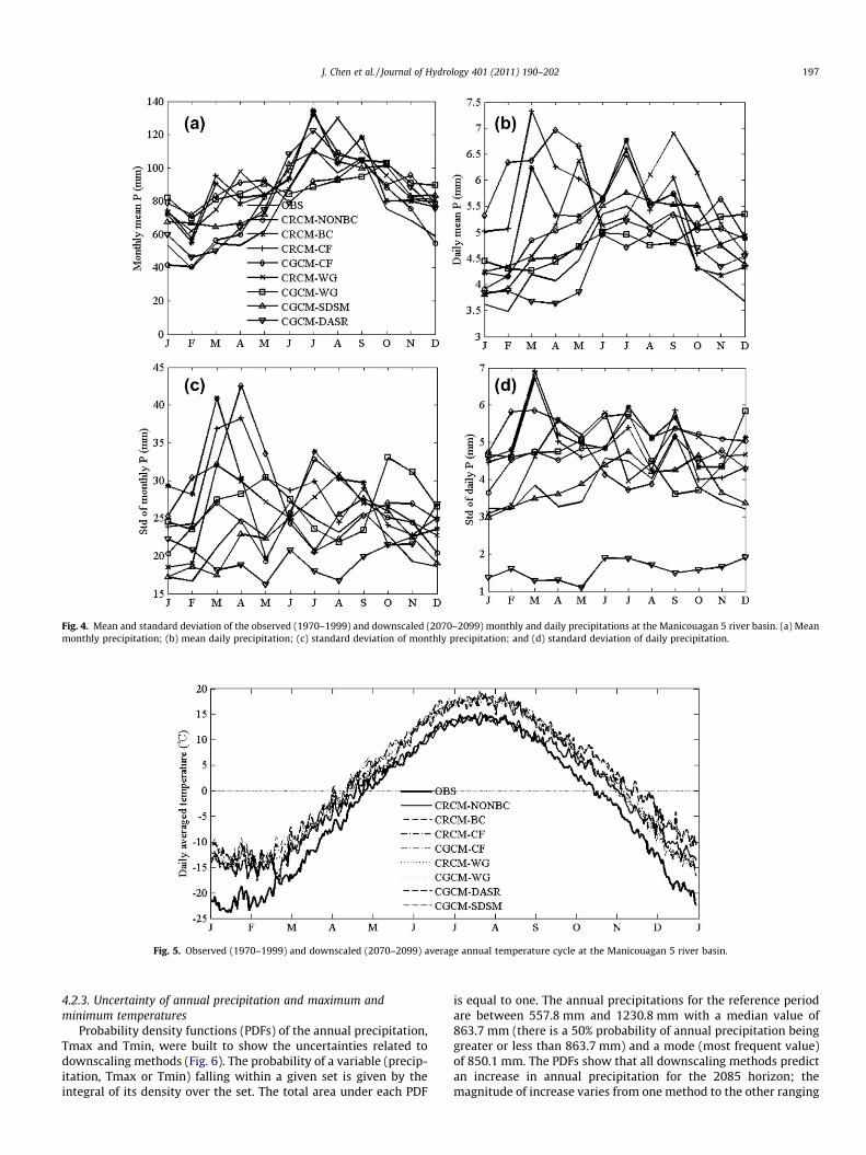
4.2.1. Monthly and daily mean precipitationsAll downscaling methods show increases in total seasonal pre-

cipitation for the 2085 horizon (Fig. 4a). The ratios of increase

ouagan 5 river basin. Observed (OBS), observed weather data simulated (OBS-SIM),rison. See Table 1 for the downscaling method acronyms.

Fig. 3. Means and standard deviations of observed (OBS) and DASR and SDSM downscaled monthly precipitations, Tmax and Tmin at the Manicouagan 5 river basin for thereference period (1970–1999).

196 J. Chen et al. / Journal of Hydrology 401 (2011) 190–202

range from 6% to 67% for spring, 1% to 20% for summer, 3% to 21%for autumn and between 5% and 45% for winter. Although bothCGCM-SDSM and CGCM-DASR are regression-based methods, theformer suggests more increases in monthly precipitation than thelatter. This is partly due to the underestimation of mean precipita-tion by the CGCM-DASR model (Fig. 3b). A bias correction is usedwith the SDSM to insure the downscaled mean precipitation agreesbetter with the observation.

The CGCM-DASR suggests 12% winter daily precipitation in-crease and 5% decrease for spring, 8% decrease for summer and2% decrease for autumn (Fig. 4b). However, the other downscalingmethods, with the exception of CGCM-WG, predict increases indaily precipitation for all seasons. The increased/decreased ratiosrange from 11% to 68% for spring, �4% (predicted by CGCM-WG)to 19% for summer, �1% (predicted by CGCM-WG) to 29% for au-tumn and between 12% and 40% for winter. The variation of dailyprecipitation in each season is not consistent with that of totallyseasonal precipitation. This is because the daily precipitation quan-tity is affected not only by the seasonal precipitation quantity, butalso by precipitation occurrence. The precipitation occurrence isdifferent for each downscaling method (results not shown).

The CGCM-DASR predicts a 26% standard deviation increase fortotal winter precipitation and a decrease for all other seasons (8%for spring, 26% for summer and 19% for autumn) for the 2085 hori-zon (Fig. 4c). This decrease is partly due to the underestimation ofthe variance of precipitation as shown in Fig. 3b. As mentioned ear-lier, the SDSM uses a stochastic component to increase downscaledvariances to better agree with observations. Other downscalingmethods suggest increases in the standard deviation of seasonalprecipitation for each season (20–59% for spring, 4–19% for sum-mer and autumn and between 18% and 50% for winter). Althoughthe CF and WG methods share similarities, the observed increases

are different, because the CF method adjusts precipitation variancethrough a modification of the mean, while WG-based methods ad-just it from changes of not only precipitation quantity but alsooccurrence. In addition, variances downscaled from CGCM andCRCM data are also different, although the CRCM is driven by theCGCM. Predicted changes in the standard deviation of daily precip-itation are not unequivocal (Fig. 4d). The CGCM-DASR suggestsreductions in the standard deviation of daily precipitation (be-tween 50% and 63% depending on the season) while the othermethods suggest increases for most of the seasons.

4.2.2. Average temperaturesFig. 5 presents annual temperature (average of Tmax and Tmin)

cycles for all downscaling methods for the 2085 horizon and forthe observed data (reference period). All of the downscalingmethods suggest increases in temperatures for the 2085 horizon.Increases range between 3.6 and 6.3 �C for spring, 0.4 and 4.1 �Cfor summer, 1.8 and 4.8 �C for autumn and between 5.7 and9.1 �C for winter. Winter temperature increases are greater thanfor other seasons. The CRCM-NONBC method suggests lower in-creases in temperature than other methods. The regression-basedstatistical methods predict a much larger increase in autumn andwinter average temperatures. Average temperature cycle graphsdisplay the freezing dates when the average temperature climbsabove and descends below zero degrees. These dates are April27th and October 15th for the reference period. Depending onthe specific downscaling method, this period could start as earlyas April 11th and as late as November 13th for the 2085 horizon,which implies that the freezing season could be shortened by upto 42 days. These changes would affect the snow accumulation inthe winter and the spring snowmelt.

Fig. 4. Mean and standard deviation of the observed (1970–1999) and downscaled (2070–2099) monthly and daily precipitations at the Manicouagan 5 river basin. (a) Meanmonthly precipitation; (b) mean daily precipitation; (c) standard deviation of monthly precipitation; and (d) standard deviation of daily precipitation.

Fig. 5. Observed (1970–1999) and downscaled (2070–2099) average annual temperature cycle at the Manicouagan 5 river basin.

J. Chen et al. / Journal of Hydrology 401 (2011) 190–202 197

4.2.3. Uncertainty of annual precipitation and maximum andminimum temperatures

Probability density functions (PDFs) of the annual precipitation,Tmax and Tmin, were built to show the uncertainties related todownscaling methods (Fig. 6). The probability of a variable (precip-itation, Tmax or Tmin) falling within a given set is given by theintegral of its density over the set. The total area under each PDF

is equal to one. The annual precipitations for the reference periodare between 557.8 mm and 1230.8 mm with a median value of863.7 mm (there is a 50% probability of annual precipitation beinggreater or less than 863.7 mm) and a mode (most frequent value)of 850.1 mm. The PDFs show that all downscaling methods predictan increase in annual precipitation for the 2085 horizon; themagnitude of increase varies from one method to the other ranging

Fig. 6. Probability density functions (PDF) of the observed (1970–1999) and downscaled (2070–2099) annual mean precipitation and maximum and minimum temperaturesat the Manicouagan 5 river basin.

198 J. Chen et al. / Journal of Hydrology 401 (2011) 190–202

between 75.0 (CRCM-NONBC) and 219.1 mm (CRCM-WG). TheCRCM-WG predicts the largest increase in annual precipitation.Medians of annual precipitation would also increase by between9% and 26% in the 2085 horizon. The CRCM-NONBC predicts thelowest increase in the median and the CRCM-WG predictsthe highest. Fig. 6a shows that an average year of precipitation inthe current climate would become a very dry year in the 2085future climate.

Each downscaling method suggests increases in annual meanTmax and Tmin for the 2085 horizon. The magnitude of the in-creases varies from one method to the other, ranging between3.6 and 5.4 �C for Tmax and between 2.4 and 5.8 �C for Tmin. Inaddition, all downscaling methods predict increases in the mediansof annual mean Tmax (3.7–5.6 �C) and Tmin (2.7–6.1 �C). TheCRCM-NONBC predicts the smallest increases in temperatures,while the two regression-based methods (CGCM-SDSM andCGCM-DASR) suggest the largest increases.

4.3. Hydrologic impacts of climate change

4.3.1. Hydrologic variablesFig. 7 presents average hydrographs simulated with precipita-

tion and temperature downscaled from the different methods. Toavoid any bias resulting from the hydrological modeling process,discharge for the reference period is represented by modeleddischarge and not by observations. The results showed that all

Fig. 7. Average annual hydrographs for the future (2070–2099) and r

downscaling methods suggest increases in winter discharge(November–April) and decreases in summer (June–October). Thetwo regression-based methods predict much larger increases inwinter flows than other methods, and, consequently, their snow-melt peak discharges are much lower. These two methods predicta larger increase in autumn and winter temperatures; the liquidwinter precipitation rapidly contributes to runoff instead of beingaccumulated in the snow cover. Thus, there is not very muchsnowmelt in spring to contribute to peak discharge. For annualdischarges, the only simulation that predicts a decrease comesfrom the CGCM-DASR method, largely because this methodunderestimates precipitation. All other downscaling methodsshow increases in annual discharges ranging between 3.5(CRCM-NONBC) and 20.9% (CRCM-WG). By the 2085 horizon, thetwo regression-based methods and the CRCM-NONBC suggest de-creases in peak discharges between 4.1% (CRCM-NONBC) and25.1% (CGCM-DASR). The slight decrease predicted by CRCM-NONBC is due to a smaller increase in annual precipitation, relativeto a larger increase in temperature. However, the CGCM-WG pre-dicts an increase in peak discharge, as do the CRCM-WG and theCRCM-BC. For these three methods, increases in winter tempera-ture are not sufficient to offset the precipitation increase. In addi-tion, for all downscaling methods the peak discharges of the 2085horizon are observed earlier than for the reference period. Lagsvary from 12 days (May 12th) for the CRCM-NONBC to 27 days(April 27) for the CGCM-CF.

eference (1970–1999) periods at the Manicouagan 5 river basin.

Fig. 8. Probability density functions (PDF) of: (a) peak discharge, (b) time to peak discharge and (c) annual mean discharge for the future (2070–2099) and reference (1970–1999) periods at the Manicouagan 5 river basin.

J. Chen et al. / Journal of Hydrology 401 (2011) 190–202 199

4.3.2. Uncertainty of hydrologic variablesIn order to better quantify the uncertainties of hydrologic vari-

ables, PDFs were constructed for peak discharge, time to peak dis-charge and annual mean discharge (Fig. 8). These graphs displaythe global uncertainty linked to downscaling techniques. Fig. 8ashows that the two regression-based methods predict the largestdecreases in peak discharges. All of the downscaling methods pre-dict an earlier peak discharge (Fig. 8b), although there is significantinter-annual variability. Inter-annual variability is very large forthe two regression-based methods as shown by their very flatPDFs. Large inter-annual variability is also shown with future an-nual mean discharge (Fig. 8c). As mentioned earlier, the CGCM-DASR method is the only that shows decreases in future annualmean discharge. The CF methods (CGCM-CF and CRCM-CF) displaythe largest future inter-annual variability of mean discharge (flat-test PDFs in Fig. 8c).

5. Discussions and conclusions

The uncertainty of climate change impacts on hydrology hasbeen given more and more attention in the scientific literature.By far the largest focus has been on investigating the roles of GCMsand GGES in the uncertainty cascade. Other sources of uncertainty,such as the choice of downscaling method, have been given muchless attention. Six downscaling methods were compared to inves-

tigate the uncertainty of downscaling methods in quantifying theimpact of climate change on the hydrology of a Canadian (Quebecprovince) River basin. The downscaling methods regroup dynami-cal and statistical approaches including the CF method and a WG-based approach. Two regression-based methods (SDSM and DASR)are also used for comparison. The downscaling methods were firstvalidated based on the modeling of discharge. Overall, all of themethods, with the exception of CGCM-DASR, result in hydrographsthat are very close to the hydrograph simulated by using observedprecipitation and temperature time series. The best methods wereCRCM data with bias correction and the SDSM. The DASR methodunderestimates the hydrograph, clearly indicating that the ex-plained variance of the linear regression approach is not sufficientto properly resolve discharge issues. The stochastic componentadded by the SDSM via bias correction and variance inflationmakes up for the basic flaw of the approach (only a small percent-age of variance is explained) with respect to precipitation.

The analysis of climate change scenarios shows that all down-scaling methods suggest increases in temperature over the basinfor the 2085 horizon. The two regression-based methods show lar-ger increases in autumn and winter temperatures than the others.Depending on the specific downscaling method, the freezing sea-son would be shortened by 26–42 days. Predicted changes in pre-cipitation are not as unequivocal as those for temperature. Resultsvary seasonally and depend on the downscaling method. The com-bined effects of precipitation and temperature changes influence

200 J. Chen et al. / Journal of Hydrology 401 (2011) 190–202

discharge differently depending on the downscaling method. Allof the methods show a general increase in winter discharge(November–April) and most show a decrease in summer discharge.Winter flows are especially large for the two regression-basedmethods, which also predict the largest temperature increases inautumn and winter. Liquid winter precipitation rapidly contributesto runoff instead of being temporarily stored in the snow cover.This leads to strongly attenuated snowmelt peak flows. Peakdischarges appear earlier for all downscaling methods, but theirtiming varies according to the downscaling method.

The results indicate that climate change impact studies basedonly on one downscaling method should be interpreted with cau-tion. General speaking, it is assumed that the major sources ofuncertainty are linked to GCMs and GGES (Kay et al., 2009; Wilbyand Harris, 2006). To make a comparison with GCM-linked uncer-tainty, the uncertainty envelope derived from the choice of down-scaling method in this paper is compared to that originating from acombination of 28 climate projections from a combination of sevenGCMs and three GGES (Fig. 9). Both uncertainty envelopes displaythe same characteristics. Downscaling contributes to a largeruncertainty in winter flows, but GCM-GGES projections give amuch larger uncertainty over the snowmelt season. Both envelopesare very similar in the summer and fall seasons. Comparing sixdownscaling methods to 28 projections (from seven GCMs to threeGGES) should contribute to a larger uncertainty envelope in thelatter case, and overall this is what was observed. On the otherhand, the two regression-based SD methods contributed propor-tionally more to the uncertainty envelope, because their behaviorwas markedly different in several instances.

The results indicated quite clearly that the choice of a down-scaling method is critical for any climate change impact study onhydrology. Can the results outlined in this paper help in selectingan appropriate method? For the most part, the answer would be‘no’ and that additional research is needed. However, these resultsdo raise some important points. It can be argued that regression-based methods should be used with caution due to their distinctivebehavior compared to other downscaling methods; their down-scaled future temperatures are very high, especially when com-pared to the direct outputs from the regional climate models(which exhibit relatively small biases in the current climate). Sodespite the fact that a high percentage of temperature variance is

Fig. 9. Envelopes of simulated discharge with: (a) six downscaling methods and (b) 28 Griver basin for the future period (2070–2099). The discharge simulated with observed c

explained by regression-based methods in the current climate,the anomalous downscaled future temperatures raise serious ques-tions about the stationary nature of the regression. This was al-ways a weak point of regression-based methods that could neverbe clearly disproved or confirmed. If there is doubt that regressionequations are stationary for temperature, the case of the validity ofthe approach for precipitation is even harder to make, mostly be-cause the percentage of explained variance is very low to beginwith. The CGCM-DASR model (a regression-based model with nobias or variance correction) was included for comparison purposesonly. It is clearly inadequate at reproducing adequate precipitationin the current climate. However, both this flawed method (CGCM-DASR) and the one correcting for precipitation bias and variance(CGCM-SDSM) give nearly identical future mean hydrographs(Fig. 7), further raising doubts as to the validity of transposingregression equations in changed climate predictions.

The strength and weaknesses of the CF method have been dis-cussed in several papers. This method gives similar results whetherfactors are derived from the GCM or the RCM (driven by the sameGCM at its boundaries). Its main weakness (that it does not modifyfuture variance and precipitation occurrence) is probably not a ma-jor obstacle with respect to spring snowmelt. Since spring floodsare the result of several months of snow accumulation followedby rapid melting, the most important feature to have in a climatechange study is the correct total quantity of solid precipitation.The variability of solid precipitation during the winter months isa less important feature to have. On the other hand, for summerand fall events, damages often result from one major rainfall event,and droughts from long periods with little to no precipitation. Insuch cases, the CF method would be totally inappropriate for cli-mate change studies and another downscaling method would benecessary. In such cases, WG based approaches may be more suc-cessful in resolving extremes series of dry days and high tempera-ture. This would especially be the case for arid and semi-arid areas.

An interesting result from this paper is that the biases in theRCM that was used are small enough that they can be dealt withby the hydrological model, thus negating any bias correction onthe outputs from the CRCM. As discussed earlier, this approachstems from the assumption that biases present in observed weath-er data (especially for precipitation) are of the same order as thosefrom the RCM precipitation. As such, a specific calibration of the

CMs and GGES using the change factor downscaling method at the Manicouagan 5limate data for the reference period (1970–1999) is also plotted for comparison.

J. Chen et al. / Journal of Hydrology 401 (2011) 190–202 201

hydrology model to each dataset is sufficient. While this hasproved to be the case in the present climate, there are large differ-ences in future predicted outflows between the direct inputs ofRCM data (CRCM-NONBC) and the use of RCM data with bias cor-rections (CRCM-BC). This is partly because CRCM precipitationused to calibrate the hydrological model (1970–1999) was drivenby initial and boundary conditions of NCEP, while it was drivenby initial and boundary conditions of CGCM for the future period(2070–2099). However, both datasets were considerably differentfor the reference period (results not shown). It should be not a sur-prise, since NCEP data and GCM data are not entirely comparable.NCEP data aims at representing the real world, whereas GCMsoperate in their own virtual world. It is difficult to say which meth-od is the most correct from both practical and theoretical view-points. The fact that they give a markedly different futurehydrology indicates that either the assumption of constant biasdoes not hold, or that the choice of different calibration parameters(in the case of CRCM-NONBC) results in significant future uncer-tainty. However, recent work (Poulin et al., 2011) demonstratesthat the uncertainty derived from hydrology model parameters isrelatively small, raising doubts toward the common assumptionof constant biases over time. Even if the direct use of RCM datahad proved to be the most interesting method, the problem re-mains that it would not be possible to sample GCM uncertaintywith this approach, as it would require outputs from several RCMs,all driven by different GCMs, over the same basin.

Clearly, more research is needed before this problem is settled.In particular, it would be interesting to get results from basins indifferent climate zones (especially arid and semi-arid climates)as the hydrological response to a choice of a given downscalingmethod may be related to a given climate. It is not possible at thisstage to recommend a specific downscaling method for a givenapplication, or even to use several downscaling methods to pro-duce an ensemble of forcings for hydrology models, such as com-monly done with GCM and GGES. Cases where the downscalinguncertainty envelope is contained within other uncertaintiessources should not be treated with the same attention than caseswhere downscaling is the main source of uncertainty. The first con-clusion of this paper is that the choice of a downscaling methoddoes matter, and that the uncertainty linked to the choice of adownscaling method should not be ignored in any climate changeimpact study. The second conclusion is that downscaling methodsare not created equal and that the choice of one or more approachshould be evaluated on a case by case basis with respect to theobjectives of the climate change impact study.

Acknowledgements

This work was partially supported by the Natural Science andEngineering Research Council of Canada (NSERC), Hydro-Québec,Manitoba Hydro and the Ouranos Consortium on climate change.The authors wish to thank Dr. Marie Minville of Hydro-Québecfor providing the program for bias correction for CRCM precipita-tion. We also gratefully acknowledge the constructive commentsof two anonymous reviewers.

References

Bardossy, A., Plate, E.J., 1992. Space time model for daily rainfall using atmosphericcirculation patterns. Water Resources Research 28, 1247–1259.

Caya, D., Laprise, R., 1999. A semi-implicit semi-lagrangian regional climate model:the Canadian RCM. Monthly Weather Review 127, 341–362.

Chen, J., Zhang, X.C., Liu, W.Z., Li, Z., 2008. Assessment and improvement of CLIGENnon-precipitation parameters for the Loess Plateau of China. Transactions of theASABE 51 (3), 901–913.

Christensen, N.S., Lettenmaier, D.P., 2007. A multimodel ensemble approach toassessment of climate change impacts on the hydrology and water resources of

the Colorado River basin. Hydrology and Earth System Sciences 11 (4), 1417–1434.

DAI CGCM3 Predictors, 2008. Sets of Predictor Variables Derived From CGCM3 T47and NCEP/NCAR Reanalysis, Version 1.1, April 2008, Montreal, QC, Canada, 15 pp.

Diaz-Nieto, J., Wilby, R.L., 2005. A comparison statistical downscaling and climatechange factor methods: impacts on low flows in the river Thanes, UnitedKingdom. Climatic Change 69, 245–268.

Duan, Q., 2003. Calibration of watershed models. In: Duan, Q., Gupta, H., Sorooshian,A.N. (Eds.), Water Science and Application, vol. 6. Washington, DC, pp. 89–104.

Fortin, V., 2000. Le modèle météo-apport HSAMI: historique, théorie et application.Institut de Recherche d’Hydro-Québec, Varennes, p. 68.

Graham, L.P., Andreasson, J., Carlsson, B., 2007a. Assessing climate change impactson hydrology from an ensemble of regional climate models, model scales andlinking methods – a case study on the Lule River basin. Climatic Change 81,293–307.

Graham, L.P., Hageman, S., Jaun, S., Beniston, M., 2007b. On interpretinghydrological change from regional climate models. Climatic Change 81, 97–122.

Hamlet, A.F., Lettenmaier, D.P., 1999. Effects of climate change on hydrology andwater resources in the Columbia River Basin. Journal of the American WaterResources Association 35 (6), 1597–1623.

Hay, L.E., Wilby, R.L., Leavesly, H.H., 2000. Comparison of delta change anddownscaled GCM scenarios for three mountainous basins in the United States.Journal of the American Water Resources Association 36 (2), 387–397.

Hostetler, S.W., 1994. Hydrologic and atmospheric models. The (continuing)problem of discordant scales. An editorial comment. Climatic Change 27 (4),345–350.

Hutchinson, M.F., McKenney, D.W., Lawrence, K., Pedlar, J.H., Hopkinson, R.F.,Milewska, E., Papadopol, P., 2009. Development and testing of Canada-wideinterpolated spatial models of daily minimum–maximum temperature andprecipitation for 1961–2003. Journal of Applied Meteorology and Climatology48, 725–741.

IPCC, Intergovernmental Panel on Climate Change, 2007. Fourth Assessment Report,Climate Change.

Kalnay, E., Kanamitsu, M., Kistler, R., Collins, W., Deaven, D., Gandin, L., Iredell, M.,Saha, S., White, G., Woollen, J., Zhu, Y., Chelliah, M., Ebisuzaki, W., Higgins, W.,Janowiak, J., Mo, K.C., Ropelewski, C., Wang, J., Leetmaa, A., Reynolds, R., Jenne,R., Joseph, D., 1996. The NCEP/NCAR 40-year reanalysis project. Bulletin of theAmerican Meteorological Society 77, 437–471.

Kay, A.L., Davies, H.N., Bell, V.A., Jones, R.G., 2009. Comparison of uncertaintysources for climate change impacts: flood frequency in England. ClimaticChange 92, 41–63.

Kilsby, C.G., Jones, P.D., Burton, A., Ford, A.C., Fowler, H.J., Harpham, C., James, P.,Smith, A., Wilby, R.L., 2007. A daily weather generator for use in climate changestudies. Environmental Modelling and Software 22 (12), 1705–1719.

Leavesley, G.H., 1994. Modeling the effects of climate change on water resources – areview. Climatic Change 28 (1–2), 159–177.

Maurer, E.P., Hidalgo, H.G., 2008. Utility of daily vs. monthly large-scale climatedata: an intercomparison of two statistical downscaling methods. Hydrologyand Earth System Sciences 12 (2), 551–563.

Minville, M., Brissette, F., Leconte, R., 2008. Uncertainty of the impact of climatechange on the hydrology of a nordic watershed. Journal of Hydrology 358, 70–83.

Minville, M., Brissette, F., Krau, S., Leconte, R., 2009. Adaptation to climate change inthe management of a Canadian water-resources system exploited forhydropower. Water Resources Management 23, 2965–2986.

Nicks, A.D., Lane, L.J., 1989. Weather Generator. In: Lane, L.J., Nearing, M.A., (Eds.),USDA–Water Erosion Prediction Project: Hillslope Profile Version. NSERL ReportNo. 2. USDA-ARS National Soil Erosion Research Laboratory, West Lafayette,Indiana, pp. 2.1–2.22 (Chapter 2).

Poulin, A., Brissette, F., Leconte, R., Arsenault, R., Malo, J.S., accepted for publication.Uncertainty of hydrological modeling in climate change impact studies. Journalof Hydrology.

Prudhomme, C., Davies, H., 2009. Assessing uncertainties in climate change impactanalyses on the river flow regimes in the UK. Part 2: future climate. ClimaticChange 93, 197–222.

Qian, B., Hayhoe, H., Gameda, S., 2005. Evaluation of the stochastic weathergenerators LARS-WG and AAFC-WG for climate change impact studies. ClimateResearch 29, 3–21.

Qian, B., Gameda, S., Jong, R., Fallon, P., Gornall, J., 2010. Comparing scenarios ofCanadian daily climate extremes derived using a weather generator. ClimateResearch 41 (2), 131–149.

Quintana Segui, P., Ribes, A., Martin, E., Habets, F., Boé, J., 2010. Comparison of threedownscaling methods in simulating the impact of climate change on thehydrology of Mediterranean basins. Journal of Hydrology 383, 111–124.

Rowell, D.P., 2006. A demonstration of the uncertainty in projections of UK climatechange resulting from regional model formulation. Climatic Change 79, 243–257.

Salathe, E.P., 2003. Comparison of various precipitation downscaling methods forthe simulation of streamflow in a Rainshadow River Basin. International Journalof Climatology 23, 887–901.

Schmidli, J., Frei, C., Vidale, P.L., 2006. Downscaling from GCM precipitation: abenchmark for dynamical and statistical downscaling methods. InternationalJournal of Climatology 26, 679–689.

Schoof, J.T., Pryor, S.C., 2001. Downscaling temperature and precipitation: acomparison of regression-based methods and artificial neural networks.International Journal of Climatology 21, 773–790.

Solman, S., Nunez, M., 1999. Local estimates of global climate change: a statisticaldownscaling approach. International Journal of Climatology 19, 835–861.

202 J. Chen et al. / Journal of Hydrology 401 (2011) 190–202

Srikanthan, R., McMahon, T.A., 2001. Stochastic generation of annual, monthlyand daily climate data: a review. Hydrology and Earth Systems Sciences 5(4), 653–670.

von Stoch, H., Zorita, E., Cubasch, U., 1993. Downscaling of global climate changeestimates to regional scales: an application to Iberian rainfall in wintertime.Journal of Climate 6, 1161–1171.

Wilby, R.L., Dawson, C.W., 2007. SDSM4.2 – A Decision Support Tool for theAssessment of Regional Climate Impacts. User Manual 1–94.

Wilby, R.L., Harris, I., 2006. A framework for assessing uncertainties in climatechange impacts: Low-flow scenarios for the River Thames, UK. Water ResourcesResearch 42, W02419. doi:10.1029/2005WR004065.

Wilby, R.L., Wigley, T.M.L., 1997. Downscaling general circulation model output: areview of methods and limitations. Progress in Physical Geography 214, 530–548.

Wilby, R.L., Hay, L.E., Leavesley, G.H., 1999. A comparison of downscaled and rawGCM output: implications for climate change scenarios in the San Juan RiverBasin, Colorado. Journal of Hydrology 225, 67–91.

Wilby, R.L., Dawson, C.W., Barrow, E.M., 2002. SDSM-A decision support tool for theassessment of regional climate change impacts. Environmental Modelling &Software 17, 145–157.

Wilby, R.L., Wigley, T.M.L., Conway, D., Jones, P.D., Hewitson, B.C., Main, J., Wilks,D.S., 1998. Statistical downscaling of general circulation model output: Acomparison of methods. Water Resources Research 34 (11), 2995–3008.

Wilks, D.S., 1995. Statistical Methods in the Atmospheric Sciences. Academic Press,New York. pp. 467.

Wilks, D.S., 1999. Multisite downscaling of daily precipitation with a stochasticweather generator. Climate Research 11, 125–136.

Wilks, D.S., 2010. Use of stochastic weather generator for precipitationdownscaling. Climate Change 1, 898–907.

Xu, C.Y., 1999. From GCMs to river flow: a review of downscaling methods andhydrologic modeling approaches. Progress in Physical Geography 23 (2), 229–249.

Xu, C.Y., Singh, V.P., 2004. Review on regional water resources assessment modelsunder stationary and changing climate. Water Resources Management 18, 591–612.

Zhang, X.C., 2005. Spatial downscaling of global climate model output for site-specific assessment of crop production and soil erosion. Agricultural and ForestMeteorology 135, 215–229.