Journal of Hydrology 491 (2013) 73–88

Contents lists available at SciVerse ScienceDirect

Journal of Hydrology

journal homepage: www.elsevier .com/ locate / jhydrol

Modeling the potential impacts of climate change on streamflowin agricultural watersheds of the Midwestern United States

0022-1694/$ - see front matter � 2013 Elsevier B.V. All rights reserved.http://dx.doi.org/10.1016/j.jhydrol.2013.03.026

⇑ Corresponding author. Tel.: +1 314 977 7654; fax: +1 314 977 3658.E-mail addresses: hchien@slu.edu (H. Chien), patyeh@rainbow.iis.u-tokyo.ac.jp

(P.J.-F. Yeh), jknouft@slu.edu (J.H. Knouft).

Huicheng Chien a, Pat J.-F. Yeh b, Jason H. Knouft c,⇑a Department of Biology, Saint Louis University, 3507 Laclede Avenue, Saint Louis, MO 63103, USAb Department of Civil and Environmental Engineering, National University of Singapore, Singaporec Department of Biology and Center for Environmental Sciences, Saint Louis University, 3507 Laclede Avenue, Saint Louis, MO 63103, USA

a r t i c l e i n f o

Article history:Received 25 October 2012Received in revised form 6 February 2013Accepted 22 March 2013Available online 1 April 2013This manuscript was handled byKonstantine P. Georgakakos, Editor-in-Chief,with the assistance of Emmanouil N.Anagnostou, Associate Editor

Keywords:Spatial streamflow variationMulti-site calibration and validationDistributed hydrologic modelingClimate change

s u m m a r y

The ability to predict spatial variation in streamflow at the watershed scale is essential to understandingthe potential impacts of projected climate change on aquatic systems in this century. However, problemsassociated with single outlet-based model calibration and validation procedures can confound the pre-diction of spatial variation in streamflow under future climate change scenarios. The goal of this studyis to calibrate and validate a distributed hydrologic model, the Soil and Water Assessment Tool (SWAT),using distributed streamflow data (1978–2009), and to assess the potential impacts of climate change onfuture streamflow (2051–2060 and 2086–2095) for the Rock River (RRW), Illinois River (IRW), KaskaskiaRiver (KRW), and Wabash River (WRW) watersheds in the Midwestern United States, primarily in Illinois.The potential impacts of climate change on future water resources are assessed using SWAT streamflowsimulations driven by projections from nine global climate models (GCMs) under a maximum of threeSRES scenarios (A1B, A2, and B1). Results from model validation indicate reasonable spatial and temporalpredictions of streamflow, suggesting that a multi-site calibration strategy is necessary to accurately pre-dict spatial variation in watershed hydrology. Compared with past streamflow records, predicted futurestreamflow based on climate change scenarios will tend to increase in the winter but decrease in thesummer. According to 26 GCM projections, annual streamflows from 2051 – 2060 (2086–2095) are pro-jected to decrease up to 45.2% (61.3%), 48.7% (49.8%), 48.7% (56.6%), and 41.1% (44.6%) in the RRW, IRW,KRW, and WRW, respectively. In addition, under the projected changes in climate, intra- and inter-annualstreamflow variability generally does not increase over time. Results suggest that increased temperaturecould change the rate of evapotranspiration and the form of precipitation, subsequently influencingmonthly streamflow patterns. Moreover, the spatially varying pattern of streamflow variability underfuture climate conditions suggests different buffering capabilities among regions. As such, regionally spe-cific management strategies are necessary to mitigate the potential impacts of climate change and pre-serve aquatic ecosystems and water resources.

� 2013 Elsevier B.V. All rights reserved.

1. Introduction

The services provided by aquatic systems are fundamentallyimportant to humans. In addition to providing clean water for con-sumption and agriculture, aquatic ecosystems sustain biodiversityand provide support for basic ecological processes as well asimportant economic activities, including fisheries and recreation.Nevertheless, aquatic systems are heavily impacted by humanactivities including land use changes associated with agricultureand urbanization, as well as physical modification to river channelswhich result in altered flow regimes (Miltner et al., 2004; Paulet al., 2006; Sullivan et al., 2006). In addition, the Earth’s climate

is predicted to exhibit significant changes in temperature and pre-cipitation during this century due to human activities (Hansenet al., 2006). These expected climatic changes have been detectedand already have resulted in measurable impacts on the physicalenvironment (IPCC, 2007).

Increased temperature is the most commonly identified issueregarding predicted changes in climate during the coming century,and the potential impacts of this warming have received themajority of attention (IPCC, 2007). Changes in precipitationpatterns are anticipated to be a significant component of climatechange as well. Modifications of precipitation patterns includingthe changes in the magnitude and temporal variability of annualprecipitation may result in relatively intense rainfallconcentrated during particular times of the year (Kattenberget al., 1996). Changes in precipitation, in combination withincreases in temperature, can have dramatic effects on the

74 H. Chien et al. / Journal of Hydrology 491 (2013) 73–88

hydrology of aquatic systems, subsequently impacting water re-sources as well as the aquatic taxa which are adapted to particularflow regimes (Poff et al., 1997).

Accurate information on the spatial variation in streamflowand the assessment of the potential impacts of climate changeon future streamflow regimes are critical for water resource man-agement, particularly in the context of water quantity, quality,and aquatic ecosystem sustainability. The coupling of hydrologicmodels with global climate models (GCMs) makes the assessmentof climate change impacts on water resources possible. Previousstudies have examined the impacts of future climate projectionsdownscaled from GCM simulations on water resources (Cher-kauer and Sinha, 2010; Hay et al., 2011; Jha et al., 2006, 2004;Kang and Ramirez, 2007; Lettenmaier et al., 1999; Nijssen et al.,2001; Takle et al., 2005). However, most of these studies have fo-cused on the change in the overall water budget rather than thespatial and temporal changes in streamflow variability. Stream-flow magnitude and variability are both essential variables influ-encing the survival, growth, and reproduction of aquatic species,and the directional alteration of these variables can impact localcommunity structure and cause populations to decline (Bainet al., 1988).

Hydrologic models used to predict future water resources underprojected warming should accurately reproduce observed stream-flow through calibration (Duan et al., 1993; Gupta et al., 1998;Sivapalan et al., 2003; Wagener et al., 2007). A significant challengein calibration is the identification of appropriate model parametersfor distributed hydrologic models. In contrast to lumped models,distributed models account for watershed spatial heterogeneityby using a relatively larger number of parameters. However, notall parameters are measureable because the scale of measurementis usually smaller than the effective scale at which the parametersare applied (Beven, 2001b).

When models are comprised of a relatively large number ofparameters, the issue of equifinality is a major concern (Beven,1993, 2001a; Lo et al., 2010, 2008). That is, multiple sets of param-eter combinations can yield similar results. Moreover, distributedhydrologic models can potentially amplify the problems associatedwith parameter estimations if spatially distributed data areunavailable for calibration. In this case, model calibration usuallyrelies on measured hydrologic responses at a single watershed out-let (Githui et al., 2009; Rouhani et al., 2007; Zhan et al., 2006), suchthat the phenomenon of ‘‘predicting the correct result for thewrong reasons’’ may occur (Jetten et al., 2003). Though distributedhydrologic models are widely used, there are still very few exten-sive calibration and validation studies against distributed groundmeasurements in both water quantity and quality modeling (Bev-en, 2002). To reduce the possibility of apparently accurate simula-tions at the watershed outlet resulting from a combination oflocally inaccurate simulations, multi-site calibration within a wa-tershed is recommended (Gul and Rosbjerg, 2010; White andChaubey, 2005; Zhang et al., 2010).

The goal of this study is to predict spatial variation of stream-flow and assess the potential impact of climate change on stream-flow in watersheds located primarily in Illinois in the MidwesternUnited States. A distributed hydrologic model, the Soil and WaterAssessment Tool (SWAT) (Arnold et al., 1998), was calibrated andvalidated with measured streamflow from multiple gauged sites.The Sequential Uncertainty Fitting Algorithm (SUFI-2) (Abbaspouret al., 2004, 2007) was used for model calibration, validation, anduncertainty analysis. After the SWAT model was calibrated andvalidated, 26 biased-corrected and spatially downscaled futureclimate projections derived from nine GCMs were used to drivethe validated SWAT model in order to assess the potential im-pacts of climate change on water resources in the studiedwatersheds.

2. Materials and methods

2.1. SWAT hydrologic model

SWAT is a physically-based and distributed hydrologic modeldeveloped to predict the impacts of changes in landscape manage-ment practices on water, sediment, and agricultural chemicalyields (Arnold et al., 1998). In addition, SWAT is capable of assess-ing the impacts of climate change on hydrologic responses andagricultural activities by adjusting climatic variables based on fu-ture projections (Arnold and Fohrer, 2005; Neitsch et al.,2005a,b). SWAT typically operates on a daily time step for long-term simulations at large watershed scales. SWAT accounts forspatial heterogeneities by first dividing a large watershed into sev-eral sub-basins, and then further dividing the sub-basins into mul-tiple hydrologic response units (HRUs). Each HRU is a combinationof unique soil, land cover and management strategies. The simu-lated water quantity and quality from each sub-basin are routedby streamflow and distributed to the watershed outlet. For a moredetailed description of SWAT, see Neitsch et al. (2005b).

2.2. Calibration and uncertainty analysis using SUFI-2

Due to the processes resulting in equifinality (Beven and Binley,1992), it is difficult to manually calibrate a distributed model inwhich there are numerous parameters influencing the simulatedhydrologic response. The SUFI-2 algorithm was used to assist mod-el calibration, validation and uncertainty analysis (Abbaspour et al.,2004, 2007). Compared with similar techniques such as the Gener-alized Likelihood Uncertainty Estimation (GLUE) (Beven and Bin-ley, 1992), Parameter Solution (ParaSol) (van Griensven andMeixner, 2006), and Bayesian inference methods (Kuczera and Par-ent, 1998), SUFI-2 requires fewer simulations to achieve a similarlevel of performance (Yang et al., 2008). Instead of identifyingabsolute parameter values, the characterization of parameterranges is more important (Bardossy and Singh, 2008). Starting withthe initial parameter ranges, SUFI-2 is capable of generating differ-ent parameter combinations, comparing simulations with observa-tions, and identifying the optimal parameter ranges. Moreover,instead of calibrating model parameters based on hydrologic re-sponses from a single watershed outlet, SUFI-2 is able to simulta-neously calibrate parameters based on distributed data within awatershed. Hydrologic models cannot avoid uncertainties originat-ing from input data, parameters, and model structures (Abbaspouret al., 2007; Dillah and Protopapas, 2000; Dubus and Brown, 2002;Leenhardt, 1995; Zhang et al., 1993). However, SUFI-2 maps alluncertainties onto the parameter ranges and quantifies overalluncertainty in the output of hydrologic response using a 95% pre-diction uncertainty (95PPU), which, in this study, was calculated atthe 2.5% and 97.5% levels of the cumulative distribution of an out-put variable obtained through the Latin hypercube sampling tech-nique (Abbaspour et al., 2007). Moreover, SUFI-2 quantifies theuncertainties using P-factor and R-factor statistics. P-factor is thepercentage of measured data falling into the 95PPU confidenceinterval, whereas R-factor is the average breadth of the 95PPU banddivided by the standard deviation of measured data. The goal ofSUFI-2 is to include the majority of measured data with the small-est possible uncertainty bands.

2.3. Study area and data

The study area consists of four watersheds: the Rock River wa-tershed (RRW), Illinois River watershed (IRW), Kaskaskia River wa-tershed (KRW), and Wabash River watershed (WRW) (Fig. 1). Allfour watersheds are located east of the Mississippi River, primarily

Fig. 1. Map of the study area indicating the locations of the climate and streamflow observation stations in the Illinois River, Kaskaskia River, Rock River, and Wabash Riverwatersheds.

H. Chien et al. / Journal of Hydrology 491 (2013) 73–88 75

cover portions of Illinois, Wisconsin, and Indiana, and drain a totalarea of 206,928 km2 (Table 1). The watershed outlets of RRW, IRW,and KRW are located at confluences with the Mississippi River,while the WRW outlet is located at the confluence of the WabashRiver and the Ohio River. Dominant soils in Illinois typically havesilt loam and silt clay loam textures (Eltahir and Yeh, 1999; Yehet al., 1998). More information on the Illinois hydrometeorologycan be found in Yeh and Famiglietti (2008, 2009).

Table 1Watershed information including the number of precipitation weather stations, temperatu

Drainage area Number of Number o

Acronym (km2) Prec stations Temp stat

Rock River watershed RRW 28401.02 33 28Illinois River watershed IRW 72985.53 78 55Kaskaskia River watershed KRW 15418.76 29 18Wabash River watershed WRW 90123.05 83 58

Prec: precipitation; Temp: temperature.

Streamflow data measured from United States Geological Sur-vey (USGS) gauging stations were used for SWAT calibration andvalidation. Average monthly streamflow data recorded from 1975to 2009 were available from 100 USGS gauging stations distributedwithin these four watersheds (Fig. 1). Three Geographic Informa-tion System (GIS) data layers were used to parameterize SWAT: agridded 30 m digital elevation model (DEM) (NED, 2000), a1:250,000 digital soil dataset from the State Soil Geographic

re weather stations, calibration stream gauge stations, drainage area, and land use.

f Number of Land use above the watershed outlet (%)

ions Calibration stations Agriculture Forest Urban Water Others

14 75.41 8.42 9.64 5.31 1.2241 71.33 12.14 12.49 2.73 1.3120 70.54 16.16 9.10 3.64 0.5625 68.54 18.94 9.32 1.85 1.35

76 H. Chien et al. / Journal of Hydrology 491 (2013) 73–88

(STATSGO2) database (NRCS, 2006), and a land use map based onthe National Land Cover Dataset (Homer et al., 2004). All GIS datawere downloaded from the United States Department of Agriculture(USDA) geospatial data gateway (http://datagateway.nrcs.usda.gov/).

2.4. Climate data

SWAT requires daily climate data, including precipitation, max-imum air temperature, minimum air temperature, solar radiation,wind speed, and relative humidity to drive the water balance mod-el. When observed climate data are not available, the stochasticweather generator model within SWAT can simulate daily weatherdata or fill in gaps of missing data based on average monthly cli-mate statistics from neighboring stations (Sharpley and Williams,1990). In this study, climate data from four sources, (1) observedclimate data from the National Weather Service (NWS) weatherstations (OBSNWS) from 1975 to 2009 (http://lwf.ncdc.noaa.gov/oa/ncdc.html), (2) gridded observed climate data compiled by theVariable Infiltration Capacity (VIC) group (OBSVIC) from 1975 to1999, (3) climate data from various GCMs from 1975 to 1999,and (4) future climate data from various GCMs from 2046 to2065 and 2081 to 2100, were used to drive SWAT (Fig. 2). OBSNWS

from 1975 to 2009, including daily precipitation and minimum andmaximum air temperature, were obtained from 223 precipitationstations and 159 temperature stations from the NWS (Fig. 1), andwere input into SWAT to drive the streamflow simulations for cal-ibration and validation. The other necessary climate variables weresimulated by the SWAT weather generator. Nine global climateprojections obtained from the online archive ‘‘Bias Corrected andDownscaled WCRP (World Climate Research Programme’s) CMIP3(Coupled Model Intercomparison Project phase 3) Climate Projec-tions’’ (Maurer et al., 2010) were used for future SWAT model pre-dictions (Appendix A). A gridded climate dataset (OBSVIC)representing 20th century surface climate conditions based onobservations and complied by the Variable Infiltration Capacitygroup (Maurer et al., 2002) was used to correct the bias of a givenGCM’s simulation of the 20th century climate (GCM20c3m). The ba-sis for bias-correction was developed by focusing on datasets ofOBSVIC and GCM20c3m at a 2� spatial resolution. The bias-correctionwas then applied to the GCM future climate projections datasets.Downscaling spatially translated bias-corrected GCM projections

Fig. 2. Schematic diagram of SWAT simulation runs with various climate data sources incobserved climate data compiled by the variable infiltration capacity (VIC) group; (3) cuGCM. Measured streamflow from 1978 to 1999 (Qobs1) and 2000–2009 (Qobs2) were use

(1961–2000, 2046–2065, 2081–2100) data from climate modelsat a 2� spatial resolution to a 1/8� resolution is more relevant towatershed-scale hydrologic modeling (Hidalgo et al., 2008; Maurerand Hidalgo, 2008; Maurer et al., 2010), thereby providing approx-imately 184, 434, 94, and 529 grid points within the RRW, IRW,KRW, and WRW, respectively. Analysis of GCM predictions alsoindicated that a bias in precipitation estimates from 2046 to2065 and from 2081 to 2100 occurred during the downscaling pro-cess, which resulted in an underestimation of precipitation inwatersheds in this study. We corrected the precipitation bias intro-duced from spatial downscaling by calculating a simple multiplica-tive scaling of average monthly precipitation for each grid betweenOBSVIC and GCM20c3m, and applying the multiplicative scaling toeach grid of downscaled GCM precipitation data from 2046 to2065 and 2081 to 2100. A simple multiplicative scaling of averagemonthly precipitation was calculated as:

Pi ¼Pi OBSVIC

Pi GCM20c3m; i ¼ 1;2; . . . 12 ð1Þ

where Pi is a multiplicative scaling of average monthly precipitationfor each month i from 1975 to 1999, Pi_OBSVIC and Pi_GCM20c3m areindividual average monthly precipitation estimates for 1975–1999from OBSVIC and GCM20c3m, respectively.Each GCM, except GCM8,is represented by three scenarios for future greenhouse gas emis-sions as defined in the IPCC Special Report on Emissions Scenarios(SRESs) (Nakicenovic and Swart, 2000). These three scenarios in-clude SRES A2 (higher emissions path), SRES A1B: (middle emis-sions path), and SRES B1 (lower emissions path). GCM8 onlyincludes the A2 and B1 scenarios (Appendix A).

2.5. Model setup and statistical analysis

The SWAT ArcGIS (version 9.3) interface (Neitsch et al., 2005a,b)was used to write SWAT input files from the DEM, soil, and landuse GIS data layers. There were 303, 805, 169, and 902 sub-basinsdelineated in RRW, IRW, KRW, and WRW, respectively. In order toreduce computational burden in large watersheds, the dominantsoil type and land use were characterized in each sub-basin. Theworkflow of SWAT simulation runs with various past and futureclimate datasets are displayed in Fig. 2. Climate data from OBSNWS

including daily precipitation, maximum air temperature, and

luding: (1) observed climate data from National Weather Service (NWS); (2) griddedrrent climate data (20c3m) from each GCM; and (4) future climate data from eachd for calibration and validation, respectively.

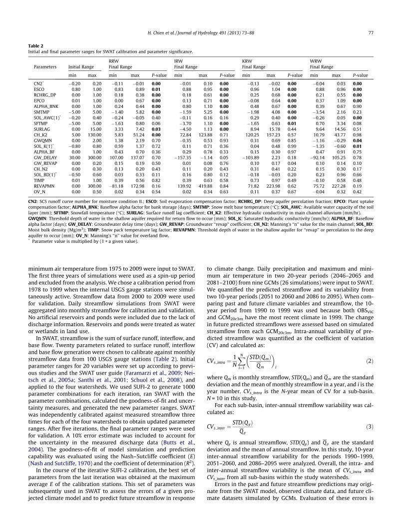
Table 2Initial and final parameter ranges for SWAT calibration and parameter significance.

RRW IRW KRW WRWParameters Initial Range Final Range Final Range Final Range Final Range

min max min max P-value min max P-value min max P-value min max P-value

CN2* �0.20 0.20 �0.11 �0.01 0.00 �0.01 0.10 0.00 �0.13 �0.02 0.00 �0.04 0.03 0.00ESCO 0.80 1.00 0.83 0.89 0.01 0.88 0.95 0.00 0.96 1.04 0.00 0.88 0.96 0.00RCHRG_DP 0.00 1.00 0.18 0.38 0.00 0.18 0.61 0.00 0.25 0.68 0.00 0.21 0.55 0.00EPCO 0.01 1.00 0.00 0.67 0.00 0.13 0.71 0.00 �0.08 0.64 0.00 0.37 1.09 0.00ALPHA_BNK 0.00 1.00 0.24 0.44 0.00 0.80 1.10 0.00 0.48 0.67 0.00 0.39 0.67 0.90SMTMP �5.00 5.00 �1.40 5.82 0.00 �1.59 5.25 0.00 �1.98 4.08 0.00 �3.54 2.16 0.23SOL_AWC(1)* �0.20 0.40 �0.24 �0.05 0.40 �0.11 0.16 0.16 0.29 0.40 0.00 �0.26 0.05 0.00SFTMP �5.00 5.00 �1.63 0.80 0.06 �3.70 1.10 0.00 �1.65 0.63 0.01 0.70 3.34 0.08SURLAG 0.00 15.00 3.33 7.42 0.03 �4.50 1.13 0.00 8.94 15.78 0.44 9.64 14.56 0.51CH_K2 5.00 130.00 5.83 51.24 0.00 72.84 123.88 0.71 120.25 157.23 0.57 10.79 43.77 0.98GWQMN 0.00 2.00 1.38 2.19 0.70 �0.35 0.53 0.93 0.31 0.69 0.85 �1.16 �0.29 0.04SOL_K(1)* �0.80 0.80 0.59 1.37 0.72 0.11 0.71 0.36 0.04 0.48 0.99 �1.35 �0.60 0.01ALPHA_BF 0.00 1.00 0.43 0.70 0.36 0.29 0.78 0.33 0.15 0.30 0.97 0.47 0.91 0.75GW_DELAY 30.00 300.00 107.00 137.07 0.70 �157.35 �1.14 0.05 �103.89 2.23 0.18 �92.14 105.25 0.78GW_REVAP 0.00 0.20 0.15 0.19 0.50 0.01 0.08 0.76 0.10 0.17 0.04 0.10 0.14 0.10CH_N2 0.00 0.30 0.13 0.20 0.43 0.11 0.20 0.43 0.31 0.41 0.22 0.15 0.30 0.17SOL_BD(1)* �0.50 0.60 0.03 0.33 0.11 0.16 0.80 0.12 �0.18 �0.03 0.20 0.23 0.96 0.66TIMP 0.01 1.00 0.39 0.56 0.82 0.39 0.63 0.58 0.73 0.97 0.49 �0.10 0.58 0.48REVAPMN 0.00 300.00 �81.18 172.98 0.16 139.92 419.88 0.84 71.82 223.98 0.62 75.72 227.28 0.19OV_N 0.00 0.50 0.02 0.34 0.54 0.02 0.34 0.63 0.11 0.37 0.67 �0.04 0.32 0.42

CN2: SCS runoff curve number for moisture condition II.; ESCO: Soil evaporation compensation factor; RCHRG_DP: Deep aquifer percolation fraction; EPCO: Plant uptakecompensation factor; ALPHA_BNK: Baseflow alpha factor for bank storage (days); SMTMP: Snow melt base temperature (�C); SOL_AWC: Available water capacity of the soillayer (mm); SFTMP: Snowfall temperature (�C); SURLAG: Surface runoff lag coefficient; CH_K2: Effective hydraulic conductivity in main channel alluvium (mm/hr).GWQMN: Threshold depth of water in the shallow aquifer required for return flow to occur (mm); SOL_K: Saturated hydraulic conductivity (mm/hr); ALPHA_BF: Baseflowalpha factor (days); GW_DELAY: Groundwater delay time (days); GW_REVAP: Groundwater ‘‘revap’’ coefficient; CH_N2: Manning’s ‘‘n’’ value for the main channel; SOL_BD:Moist bulk density (Mg/m3); TIMP: Snow pack temperature lag factor; REVAPMN: Threshold depth of water in the shallow aquifer for ‘‘revap’’ or percolation to the deepaquifer to occur (mm); OV_N: Manning’s ‘‘n’’ value for overland flow.* Parameter value is multiplied by (1 + a given value).

H. Chien et al. / Journal of Hydrology 491 (2013) 73–88 77

minimum air temperature from 1975 to 2009 were input to SWAT.The first three years of simulations were used as a spin-up periodand excluded from the analysis. We chose a calibration period from1978 to 1999 when the internal USGS gauge stations were simul-taneously active. Streamflow data from 2000 to 2009 were usedfor validation. Daily streamflow simulations from SWAT wereaggregated into monthly streamflow for calibration and validation.No artificial reservoirs and ponds were included due to the lack ofdischarge information. Reservoirs and ponds were treated as wateror wetlands in land use.

In SWAT, streamflow is the sum of surface runoff, interflow, andbase flow. Twenty parameters related to surface runoff, interflowand base flow generation were chosen to calibrate against monthlystreamflow data from 100 USGS gauge stations (Table 2). Initialparameter ranges for 20 variables were set up according to previ-ous studies and the SWAT user guide (Faramarzi et al., 2009; Nei-tsch et al., 2005a; Santhi et al., 2001; Schuol et al., 2008), andapplied to the four watersheds. We used SUFI-2 to generate 1000parameter combinations for each iteration, ran SWAT with theparameter combinations, calculated the goodness-of-fit and uncer-tainty measures, and generated the new parameter ranges. SWATwas independently calibrated against measured streamflow threetimes for each of the four watersheds to obtain updated parameterranges. After five iterations, the final parameter ranges were usedfor validation. A 10% error estimate was included to account forthe uncertainty in the measured discharge data (Butts et al.,2004). The goodness-of-fit of model simulation and predictioncapability was evaluated using the Nash–Sutcliffe coefficient (E)(Nash and Sutcliffe, 1970) and the coefficient of determination (R2).

In the course of the iterative SUFI-2 calibration, the best set ofparameters from the last iteration was obtained at the maximumaverage E of the calibration stations. This set of parameters wassubsequently used in SWAT to assess the errors of a given pro-jected climate model and to predict future streamflow in response

to climate change. Daily precipitation and maximum and mini-mum air temperature in two 20-year periods (2046–2065 and2081–2100) from nine GCMs (26 simulations) were input to SWAT.We quantified the predicted streamflow and its variability fromtwo 10-year periods (2051 to 2060 and 2086 to 2095). When com-paring past and future climate variables and streamflow, the 10-year period from 1990 to 1999 was used because both OBSVIC

and GCM20c3m have the most recent climate in 1999. The changein future predicted streamflows were assessed based on simulatedstreamflow from each GCM20c3m. Intra-annual variability of pre-dicted streamflow was quantified as the coefficient of variation(CV) and calculated as:

CVs intra ¼1N

XN

i¼1

STDðQmÞQ m

� �i

ð2Þ

where Qm is monthly streamflow, STD(Qm) and Qm are the standarddeviation and the mean of monthly streamflow in a year, and i is theyear number. CVs_intra is the N-year mean of CV for a sub-basin.N = 10 in this study.

For each sub-basin, inter-annual stremflow variability was cal-culated as:

CVs inter ¼STDðQyÞ

Q y

ð3Þ

where Qy is annual streamflow, STD(Qy) and Qy are the standarddeviation and the mean of annual streamflow. In this study, 10-yearinter-annual streamflow variability for the periods 1990–1999,2051–2060, and 2086–2095 were analyzed. Overall, the intra- andinter-annual streamflow variability is the mean of CVs_intra andCVs_inter from all sub-basins within the study watersheds.

Errors in the past and future streamflow predictions may origi-nate from the SWAT model, observed climate data, and future cli-mate datasets simulated by GCMs. Evaluation of these errors is

78 H. Chien et al. / Journal of Hydrology 491 (2013) 73–88

made by comparing SWAT simulations with measured streamflowrecords (Jha et al., 2004). The possible error sources from SWATand the climate datasets are listed in Table 3. The magnitude ofthe errors was evaluated by calculating the following bias and rootmean square error (RMSE):

Bias ¼ 1N

XN

i¼1

Q s i � Q m ið Þ ð4Þ

RMSE ¼

ffiffiffiffiffiffiffiffiffiffiffiffiffiffiffiffiffiffiffiffiffiffiffiffiffiffiffiffiffiffiffiffiffiffiffiffiffiffiffiffiffi1N

XN

i¼1

ðQ s i � Q m iÞ2vuut ð5Þ

where Qm and Qs are the measured and simulated streamflow onmonth i, respectively, and N is the number of years of streamflowdata. The bias provides a measure of annual mean error betweensimulations and observations. The RMSE gives an estimate of thevariability between model simulations and observations, which isused to assess the validity of the model in reproducing the seasonalcycle. Errors were evaluated using observed and simulated stream-flow from the following stream gauges: Rock River near Joslin, IL(USGS 05446500), Illinois River at Valley City, IL (USGS05586100), Kaskaskia River near Venedy station, IL (USGS05594100), and Wabash River at Mt. Carmel, IL (USGS 03377500).

3. Results

3.1. Parameter ranges during calibration

For each watershed, although the initial parameter ranges areidentical, the optimal parameter ranges from calibration are differ-ent (Table 2). For example, the initial range of CN2 (SCS runoffcurve number for moisture condition II) is �0.2 to 0.2 for all water-sheds, but the final range is �0.11 to �0.01, �0.01 to 0.10, �0.13 to�0.02 and �0.04 to 0.03 for RRW, IRW, KRW and WRW, respec-tively (Table 2). Similar results are found for other parameters (Ta-ble 2). Not all of the 20 parameters are consistently important forthe accurate simulation of streamflow among watersheds, only thefollowing four parameters are found to be sensitive in all fourwatersheds: CN2, ESCO (soil evaporation compensation factor),RCHRG_DP (deep aquifer percolation fraction), and EPCO (plant up-take compensation factor).

3.2. SWAT calibration and validation

Simulated monthly total streamflow from SWAT is in reason-able agreement with the measurements from the 100 USGS gaugestations (Fig. 3). During the calibration, the R2 of 90% of the sta-tions, as well as the coefficient E of 77% of the stations, exceeded0.6. The number of stations with R2 and E over 0.6 decreases to78% and 71%, respectively, during the validation period (Fig. 3).More than 60% of the measurements bracketed within the 95PPUare found at 80% of the stations during calibration and 47% duringvalidation. The R-factor is below 0.8 at 87% of the stations in thecalibration, while it decreases to 57% of the stations during valida-tion (Fig. 4).

Table 3The sources of error in simulated streamflow from SWAT and climate models.*

Comparisons Error source

1 Qsim1 versus Qobs1 OBSNWS + SWAT2 Qsim3 versus Qobs1 OBSVIC + SWAT3 Qsim4 versus Qsim3 GCM4 Qsim5 versus Qsim4 Climate change

* Qsim and Qobs are simulated and observed streamflows represented in Fig. 2.

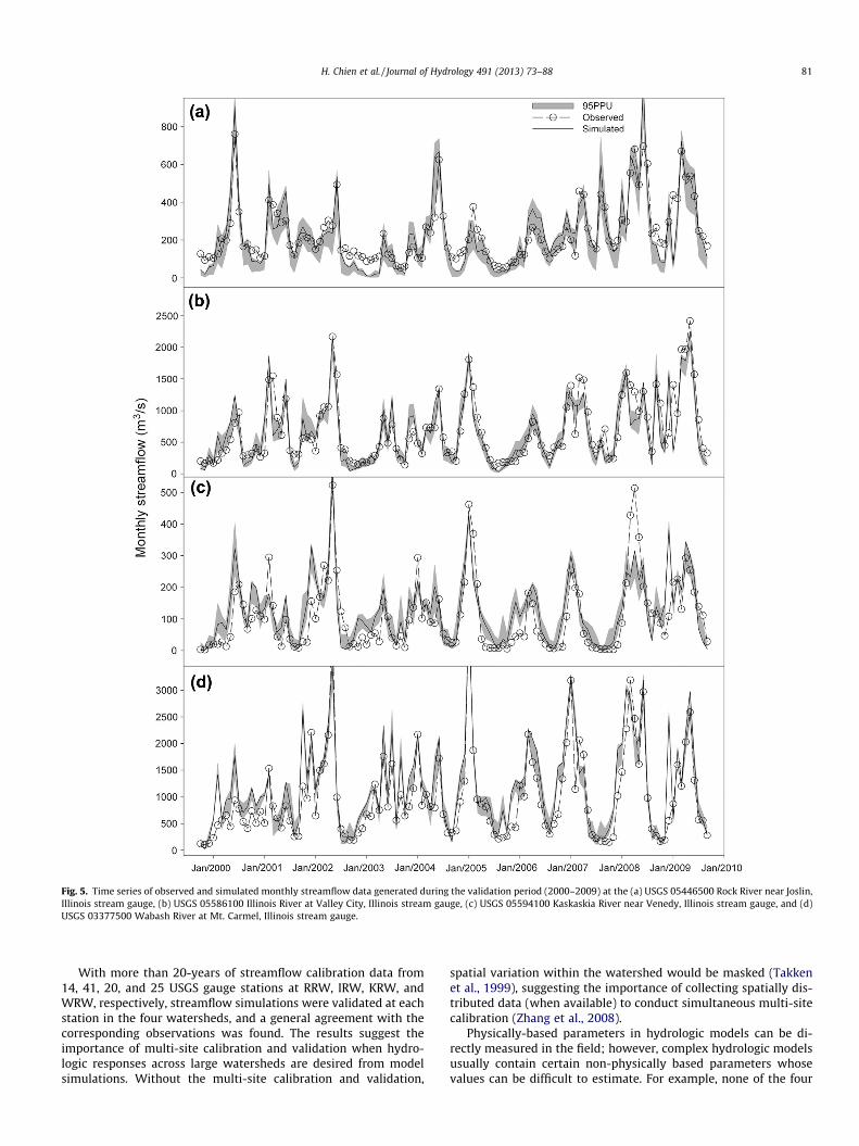
Generally, SWAT accurately reproduces long-term mean sea-sonality and month-to-month variability of hydrologic responsesas well as short-term dynamics of individual events, as indicatedby the optimal E of 0.53, 0.78, 0.75, and 0.76 during the calibrationperiod for the RRW, IRW, KRW and WRW, respectively. Accordingto the parameter ranges obtained from the calibration process ofSWAT, predicted streamflow during the validation period exhibitsa reasonable reproduction of the dynamics of the observed stream-flow during events and between events (Fig. 5). The optimal E val-ues in the validation period are 0.68, 0.71, 0.81, and 0.72 in theRRW, IRW, KRW and WRW, respectively.

3.3. Predicted streamflow from 2051 to 2060 and 2086 to 2095

In order to evaluate the impact of climate change on the spatialvariability of streamflow, we first compared 1990–1999 climateconditions from the OBSVIC and GCM20c3m data. Average annualtemperature from the OBSVIC dataset is well reproduced by thenine GCM20c3m estimates. The maximum differences in mean tem-perature between OBSVIC and GCM20c3m are 0.34 �C, 0.26 �C, 0.14 �Cand 0.26 �C in the RRW, IRW, KRW, and WRW, respectively. Annualprecipitation of OBSVIC was well matched by the nine GCM20c3m

estimates, with errors of approximately ±1%. The future mean tem-perature in 2051–2060 and 2086–2095 increases in comparisonwith the past mean temperature in 1990–1999. The mean temper-ature differences between 26 GCM projections for 2051–2060(2086–2095) and the 1990–1999 temperature are +3.05 �C(+4.57 �C), +2.64 �C (+4.09 �C), +3.27 �C (+4.72 �C), and +3.22 �C(+4.68 �C) in the RRW, IRW, KRW, and WRW, respectively. The per-centage changes of annual precipitation from 1990–1999 to 2051–2060 range from �17.98% to 7.25%, �22.98% to 6.91%, �27.58% to�5.31%, and �18.64% to 7.73%, in the RRW, IRW, KRW, and WRW,respectively. The percentage changes in annual precipitation from1990–1999 to 2086–2095 range from �24.22% to 13.16%, �22.09%to 15.48%, �33.09% to �0.08% and �21.02% to 16.17%, in the RRW,IRW, KRW and WRW, respectively.

The SWAT-predicted monthly average streamflows produced bythe 26 GCM projections indicates a wide range of potential flow re-gimes (Fig. 6). Generally, the simulated 2051–2060 and 2086–2095streamflows from the 26 GCM projections converge during sum-mer, but exhibit wider ranges during winter. For example, therange of the projected 2051–2060 streamflows among GCM projec-tions is 13.71 mm/month in August (maximum 15.77 mm/monthand minimum 2.07 mm/month), but increases to 42.28 mm/monthin December (maximum 55.17 mm/month and minimum12.89 mm/month) (Fig. 6a, KRW). However, the relative changesof projected streamflows during the summer do not representsmaller percent ranges compared with 1990–1999 simulationsfrom each GCM20c3m. For example, the relative range of the pro-jected 2051–2060 streamflow is from �80.28% to 57.69% in Augustand from �64.11% to 94.10% in December (Fig. 6a, KRW). Overall17, 17, 20, and 18 of 26 predicted annual streamflows in theRRW, IRW, KRW, and WRW, respectively, are predicted to decreasein 2051–2060 compared with the simulated streamflow from indi-vidual GCM20c3m estimates. During 2086–2095, 18, 15, 20, and 16of 26 predicted annual streamflows in RRW, IRW, KRW, andWRW, respectively, are predicted to decrease relative to GCM20c3m

estimates. The annual streamflows for 2051–2060 (2086–2095) areprojected to decrease up to 45.2% (61.3%), 48.7% (49.8%), 48.7%(56.6%), and 41.1% (44.6%) in RRW, IRW, KRW, and WRW, respec-tively (Appendix B).

3.4. Intra-annual and inter-annual streamflow variability

The majority of simulations indicate that intra-annual and inter-annual streamflow variability will decrease in the future (Table 4).

Fig. 3. The coefficient of determination (R2) for the (a) calibration and (b) validation as well as the Nash–Sutcliff coefficient for the (c) calibration and (d) validation calculatedat each of the 100 stream gauge stations.

H. Chien et al. / Journal of Hydrology 491 (2013) 73–88 79

Spatially averaged intra-annual CV in 1990–1999 is 0.99, which ishigher than 21 of the 26 estimates of the intra-annual CV in2086–2095. None of the intra-annual CV estimates in 2051–2060are higher than the 1990–1999 measure. The spatially averaged in-tra-annual CV for the 1990–1999 period using OBSNWS data is 0.71,0.97, 1.18, and 1.10 in RRW, IRW, KRW, and WRW, respectively.However, the CV for 2051–2060 (2086–2095) period decreases to0.44 (0.48), 0.90 (0.97), 0.99 (1.07), and 0.86 (0.94) in RRW, IRW,KRW, and WRW, respectively (Appendix C). Approximately 51% ofsub-basins have CV estimates greater than 1.0 during 1990–1999(Fig. 7a). Under the highest CV from the 26 GCM projections,approximately 51% of the sub-basins have intra-annual CV greaterthan 1.0 during 2051–2060 (Fig. 7b). The percentage of sub-basinswith intra-annual CV estimates greater than 1.0 increases to 85% in2081–2096 (Fig. 7c). The spatially averaged inter-annual stream-flow CV is 0.43 during 1990–1999. Only two of the 26 inter-annualstreamflow CV estimates are larger than 0.43 during 2051–2060and 2086–2095.

3.5. Uncertainty of model simulations

The levels of uncertainty of the SWAT streamflow simulationswere calculated by comparing the SWAT simulated streamflowfrom OBSNWS, OBSVIC, and OBS20c3m (Table 5). A positive value ofbias indicates an overestimation of SWAT streamflow simulations,while a negative value indicates an underestimation. The highestpercentage of biases is found for OBSNWS (�15.0%) and OBSVIC

(15.0%) (Table 5). The GCM3 exhibited the highest percentage ofbiases with an average overprediction of contemporary streamflowof 13.4%, 12.3%, 11.9%, and 13.7%, in the RRW, IRW, KRW, andWRW, respectively (Table 5).

The measure of biases in GCM-based future streamflow predic-tions is the difference between current and future streamflow sim-ulations based on various GCM projection datasets (Jha et al.,2004). Simulated streamflows from various future GCM estimatesgenerally exhibit a relatively higher percentage of bias comparedto comparisons between observed contemporary climate data

Fig. 4. P-factor scores derived from the (a) calibration and (b) validation of models at each of the 100 gauge stations as well as R-factor scores derived from the (c) calibrationand (d) validation of models at each of the 100 stream gauge stations.

80 H. Chien et al. / Journal of Hydrology 491 (2013) 73–88

and GCM20c3m (Fig. 8). Predicted future streamflows based on var-ious GCM3 projections (A2, A1B, B1) result in, on average, the high-est percentage of absolute bias, ranging from 48% to 53% amongthe four watersheds. However, the percentage of highest absolutebias is approximately 61% from GCM6 in the RRW (Fig. 8). Themajority of future streamflow predictions based on GCM projec-tions during the 2051–2060 and 2086–2095 periods indicate over-all reductions in streamflow. However, a predicted increase instreamflow is found when using the climate data projected byGCMs 1, 2 and 9 (Fig. 8).

4. Discussion

4.1. SWAT calibration and validation

The simulated streamflows produced by SWAT are generallyconsistent with observations from the four watersheds duringthe calibration and validation periods. Only three of 100 gauge

stations have negative E values. The low goodness-of-fit betweenobservations and simulations could result from any combinationof errors from observed and simulated streamflow, climate data,and/or geophysical GIS data including land use and soil maps.However, the influence of poor simulations from these three sta-tions declines with the distance downstream. When a poorlysimulated streamflow is routed downstream, the agreement be-tween simulated and observed streamflow is expected to de-crease due to error propagation (Abbaspour et al., 2007; Dillahand Protopapas, 2000; Dubus and Brown, 2002; Leenhardt,1995; Zhang et al., 1993). However, most E values in down-stream stations remain between 0.6 and 1.0 in the four water-sheds, suggesting error propagation is masked or the influenceof error from upstream stations with low goodness-of-fit esti-mates is small. The results imply the existence of hydrologic er-ror compensation (Cao et al., 2006), in which the combination ofpoorly simulated streamflow from upstream sub-basins mayyield reasonable results at downstream sub-basin and watershedoutlets.

Fig. 5. Time series of observed and simulated monthly streamflow data generated during the validation period (2000–2009) at the (a) USGS 05446500 Rock River near Joslin,Illinois stream gauge, (b) USGS 05586100 Illinois River at Valley City, Illinois stream gauge, (c) USGS 05594100 Kaskaskia River near Venedy, Illinois stream gauge, and (d)USGS 03377500 Wabash River at Mt. Carmel, Illinois stream gauge.

H. Chien et al. / Journal of Hydrology 491 (2013) 73–88 81

With more than 20-years of streamflow calibration data from14, 41, 20, and 25 USGS gauge stations at RRW, IRW, KRW, andWRW, respectively, streamflow simulations were validated at eachstation in the four watersheds, and a general agreement with thecorresponding observations was found. The results suggest theimportance of multi-site calibration and validation when hydro-logic responses across large watersheds are desired from modelsimulations. Without the multi-site calibration and validation,

spatial variation within the watershed would be masked (Takkenet al., 1999), suggesting the importance of collecting spatially dis-tributed data (when available) to conduct simultaneous multi-sitecalibration (Zhang et al., 2008).

Physically-based parameters in hydrologic models can be di-rectly measured in the field; however, complex hydrologic modelsusually contain certain non-physically based parameters whosevalues can be difficult to estimate. For example, none of the four

Fig. 6. Simulated streamflow using OBSVIC and GCM20c3m from 1990 to1999 (solid line) and simulated streamflow for: (a) 2051–2060, and (b) 2086–2095 from GCMs with A2(red), A1B (green) and B1 (blue) scenarios in absolute values (top) and relative to simulations (bottom) in Rock River (RRW), Illinois River, (IRW), Kaskaskia River (KRW), andWabash River (WRW) watersheds. (For interpretation of the references to color in this figure legend, the reader is referred to the web version of this article.)

82 H. Chien et al. / Journal of Hydrology 491 (2013) 73–88

most sensitive parameters (CN2, ESCO, RCHRG_DP, and EPCO)identified in this study are physically based. As a proxy of hydro-logic processes, the results imply that water fluxes in surface,groundwater, and evapotranspiration would be the primary prior-ities for data collection for conducting multi-site calibration andvalidation in relatively large watersheds.

4.2. Predicted streamflow

With 26 bias-corrected and downscaled climate projections forthe periods 2051–2060 and 2086–2095, our results suggest thatannual streamflow will likely decrease based on the majority ofGCM-based SWAT model simulations. However, the monthly

Table 4The mean of intra-annual and inter-annual streamflow variability, quantified as coefficientFor periods 2051–2060 and 2086–2095, the highest, lowest and median CV is presented f

1990–1999 2051–2060

CV Highest_CV Lowest_CV

Intra-annual 0.9969 0.9925 0.6299Inter-annual 0.4343 0.4943 0.1711

streamflow pattern is altered throughout the year. The results sug-gest that streamflow will tend to increase in winter but decrease insummer for both future time periods. The altered pattern ofmonthly streamflow is more obvious in KRW and WRW, whichare located in the southern part of the study region. This alteredstreamflow pattern is potentially driven by changes in the waterbudget including alteration of evapotranspiration induced bychanges in precipitation and temperature. Warmer temperaturesmay also play an additional role in the alteration of streamflowpatterns. When the temperature is warmer in winter, precipitationmore frequently falls as rain instead of snow, which could explainwhy reduced precipitation in January and February can still resultin higher streamflow in the four watersheds.

of variation (CV), in the four watersheds for 1990–9999, 2051–2060, and 2086–2095.rom 26 GCM projections.

2086–2095

Median_CV Highest_CV Lowest_CV Median_CV

0.8442 1.3204 0.7138 0.75230.3083 0.6397 0.2261 0.3029

Fig. 7. Coefficient of variation (CV) of the (a) 1990 to 1999, (b) 2051–2060 highest, and (c) 2086–2095 highest simulated intra-annual streamflow variability in each sub-basin.

Table 5Estimated errors from SWAT simulations based on observed (OBSNWS and OBSVIC) and GCM (GCM20c3m) climate data from 1990 to 1999.

Error GCM RCW IRW KRW WRW

Bias RMSE Bias RMSE Bias RMSE Bias RMSE

mm (%) mm mm (%) mm mm (%) mm mm (%) mm

OBSNWS + SWAT �21.8 (�7.4) 4.50 �55.9 (�15.0) 5.34 �6.3 (�2.1) 5.69 �5.2 (�1.4) 4.68OBSVIC + SWAT 44.5 (15.0) 6.80 �0.5 (�0.1) 4.08 28.1 (9.2) 6.37 45.1 (12.0) 6.43GCM20c3m GCM1 9.2 (2.7) 4.82 6.6 (1.8) 9.30 5.0 (1.5) 10.02 9.4 (2.2) 8.73

GCM2 �6.1 (�1.8) 5.25 �29.3 (�7.9) 9.89 �34.5 (�10.3) 9.96 �12 (�2.9) 7.81GCM3 45.6 (13.4) 6.02 45.8 (12.3) 7.31 39.9 (11.9) 7.82 57.6 (13.7) 7.57GCM4 5.9 (1.8) 4.46 14.5 (3.9) 8.17 23.6 (7.1) 9.45 24.3 (5.8) 6.96GCM5 �13.1 (�3.8) 5.27 �15.9 (�4.3) 9.14 �12.5 (�3.5) 6.88 �3.8 (�0.9) 8.18GCM6 �11.5 (�3.4) 4.79 �24.7 (�6.6) 7.74 �13.5 (�4.2) 6.95 �18 (�4.3) 6.38GCM7 �5.6(�1.6) 6.20 �3.6 (�0.8) 11.55 5.1 (1.5) 10.11 11.5 (2.7) 9.79GCM8 4.6 (1.3) 3.65 4.2 (1.1) 7.41 �1.7 (�0.5) 10.02 4.3 (1.0) 7.86GCM9 �18.4 (�5.4) 5.32 �26.3 (�7.1) 8.88 �9.3 (�2.8) 9.32 �14.5 (�3.4) 8.09

H. Chien et al. / Journal of Hydrology 491 (2013) 73–88 83

Precipitation is predicted to be relatively high in July and Au-gust by most GCM projections; however, the streamflow is pre-dicted to be relatively low in these two months. This resultsuggests that the annual streamflow may be dominated by precip-itation, but warmer temperatures could change the rate of evapo-transpiration, subsequently influencing monthly streamflowpatterns (Islam et al., 2012). Previous studies have indicated simi-lar relationships between rising air temperature and decreased

streamflow (Chen et al., 2007; Hawkins and Austin, 2012; Najjaret al., 2010; Tang et al., 2012).

4.3. Streamflow variability

Our results indicate that the majority of simulated streamflowfrom the 26 GCM projections from 2051 – 2060 and from 2086to 2095 exhibit lower variability in terms of intra- and inter-annual

Fig. 8. Bias percentage of predicted streamflow from 2051 to 2060 and 2086 to 2095 in comparison to simulated streamflow from GCM20c3m.

84 H. Chien et al. / Journal of Hydrology 491 (2013) 73–88

CV compared with that during 1990–1999. Streamflow variabilityis primarily influenced by factors including frequency and magni-tude of precipitation and land use and land cover characteristics(Chang et al., 2012; Nippgen et al., 2011). In this study, land useand land cover were not changed during SWAT simulations forperiods 1990–1999, to 2051–2060 and 2086–2095, which limitschanges in climate as the primary factor influencing changes instreamflow variability.

The analyses of streamflow variability (CV) suggests that dif-ferent regions have different buffering capabilities in response topotential climate change scenarios (Hay et al., 2011; Roots,1989). A plausible explanation is that the hydrologic responsein a given watershed may be dominated by different hydrologicprocesses (Grayson and Blöschl, 2000; Sivakumar, 2004, 2008).Previous studies indicate that total rainfall, rainfall intensity,and soil water are dominant variables driving hydrologic pro-cesses in agricultural watersheds (Houser et al., 2000). Tempera-ture is the dominant variable for stream discharge in middle- tohigh-latitude watersheds where snow tends to accumulate dur-ing the winter (Liu et al., 2007; Nijssen et al., 2001). With cli-mate change, in terms of increased temperature and alteredprecipitation patterns, the response to climate change in snow-covered areas may be more severe than in warmer regions be-cause of extreme hydrologic events associated with snowmelt.The increased temperature would result in relatively greaterchanges in snowmelt in winter or earlier spring and subse-quently cause more soil moisture to evaporate. Even withinthe same watershed, different land-use types may differentiallyinfluence the hydrologic response to climate change. For exam-

ple, forests (as opposed to agricultural landscapes) could bettermitigate the impact of intense precipitation by limiting theamount of soil erosion from the land surface (Nearing et al.,2005; Schiettecatte et al., 2008). The results from this study sug-gest that different strategies are likely required in different re-gions in response to anticipated climate change.

4.4. Uncertainties in climate change impact

Climate data from OBSVIC were compiled from the NationalWeather Service COOP database. Maurer et al. (2002) developedthe OBSVIC according to the daily precipitation and maximumand minimum temperature of OBSNWC and gridded these datainto a 1/8� spatial resolution using the synergraphic mappingsystem algorithm. The uncertainty of SWAT simulations com-bined with that of OBSNWS or OBSVIC provides a threshold thatcan be compared to uncertainties arising from using differentGCM climate projection data. The bias percentage from SWATcombined with OBSNWS or OBSVIC is estimated to be between±15%, which suggests uncertainties from GCM initial conditions(GCM20c3m) are reasonable. However, the bias percentage frommost of the 26 GCM projections is greater than ±15% (Fig. 8).These results suggest dramatic changes in streamflow in the fu-ture, with most cases indicating reductions in streamflow. Inaddition, the variability among future streamflow predictions im-plies that the selection of future projections from climate modelsimulations critically affects the prediction of water yield underclimate change (Stone et al., 2003).

H. Chien et al. / Journal of Hydrology 491 (2013) 73–88 85

Based on uncertainty analyses using Bias and RMSE, anexpectation of decreased future streamflow and streamflowvariability is reasonable. However, future streamflow esti-mates in this study are based on predicted changes in precip-itation and temperature. Human activities, particularly relatedto land transformations, may also have significant impacts onthe hydrologic cycle in these watersheds. Therefore, theintegration of projected land use changes in futurehydrologic modeling studies may help to refine streamflowpredictions.

5. Conclusions

We used the SWAT distributed hydrologic model in combina-tion with the SUFI-2 multi-site calibration procedure to demon-strate that spatial and temporal variation in streamflow overlarge watersheds can be reasonably represented through multi-sitecalibration and validation. Without the availability of distributedhydrologic data for calibration and validation, distributed hydro-logic models are best characterized as lumped models. Distributedhydrologic models are more complex than lumped models in termsof their structure and number of parameters. However, not allmodel parameters are sensitive to the simulations of hydrologic re-sponses, thereby providing the opportunity to reduce the numberof calibration parameters in the distributed models. Among the20 parameters calibrated, only four parameters are found to besensitive in all four watersheds, suggesting the importance of mul-ti-site calibration and validation across relatively large spatialscales.

Many of the difficulties and limitations during calibrationand validation were data related. We used multi-site stream-flow data to calibrate and validate the SWAT. However, stream-flow is only one of the components of the water cycle, andthese data are widely available compared with other aspectsof the water cycle, such as evapotranspiration and soil mois-ture. Soil moisture data should eventually be available acrossIllinois, thus offering the opportunity to refine modelpredictions.

The coupling of hydrologic models and GCM projections al-lows for the prediction of future streamflow conditions. Usingclimate model projections to drive the distributed hydrologicsimulations, our results suggest the potential for dramaticchanges in streamflow as well as streamflow variability duringthe coming century in most watersheds in Illinois and adjacentmidwestern states. In particular, annual streamflows for 2051–2060 (2086–2095) could decrease up to 45.2% (61.3%), 48.7%(49.8%), 48.7% (56.6%), and 41.1% (44.6%) in the RRW, IRW,KRW, and WRW, respectively, while the intra-annual stream-flow variability will likely decrease in all watersheds in theperiods of 2051–2060 and 2086–2095 compared to that in1990–1999. Such predictions of hydrologic response to the pro-jected changes in future climate may provide the foundationfor water management strategies focused on the mitigation ofthe impacts of climate change on aquatic resources andecosystems.

Acknowledgements

We thank the Program for Climate Model Diagnosis and Inter-comparison (PCMDI) and the WCRP’s Working Group on CoupledModelling (WGCM) for providing the WCRP CMIP3 multi-model

dataset. We also thank M. Anthony, C. Beachum, M. Chu, M. Michel,S. Niu, and two anonymous reviewers for providing extremelyhelpful comments on a previous version of this manuscript.Funding for this research was provided to JHK by the Environmen-tal Protection Agency’s (EPAs) Science to Achieve Results (STARs)Consequences of Global Change for Water Quality program (EPA-G2008-STAR-D2) and from the National Science Foundation(DEB-0844644).

Appendix A.

The GCM model groups, model designation, and acronym. EachGCM has three SRES scenarios for future greenhouse gas emissionsforcing global climate. The three SRES scenarios are A2 (higher’’emissions path), A1B (‘‘middle’’ emissions path), and B1 (‘‘lower’’emissions path). GCM8 only has A2 and B1 scenarios. When theGCM has multiple simulations featuring unique initial conditionsto simulate future climate projections, only the first run wasused.

Modeling group

IPCC modeldesignation

Acronym

1

Canadian Centre for ClimateModeling and Analysis

CGCM3.1(T47)

GCM1

2

Meteo-France/Centre Nationalde RecherchesMeteorologiques, France

CNRM-CM3

GCM2

3

US Dept. of Commerce/NOAA/Geophysical Fluid DynamicsLaboratory, USA

GFDL-CM2.0

GCM3

4

US Dept. of Commerce/NOAA/Geophysical Fluid DynamicsLaboratory, USA

GFDL-CM2.1

GCM4

5

Institute Pierre Simon Laplace,France

IPSL-CM4

GCM5

6

Center for Climate SystemResearch (The University ofTokyo), National Institute forEnvironmental Studies, andFrontier Research Center forGlobal Change (JAMSTEC),Japan

MIROC3.2(medres)

GCM6

7

Meteorological Institute of theUniversity of Bonn,Meteorological ResearchInstitute of KMA

ECHO-G

GCM7

8

Max Planck Institute forMeteorology, Germany

ECHAM5/MPI-OM

GCM8

9

Meteorological ResearchInstitute, Japan

MRI-CGCM2.3.2

GCM9

Appendix B.

Predicted annual streamflows for three periods 1990–1999,2051–2060 and 2086–2095 in the RRW, IRW, KRW, and WRWbased on climate inputs from nine GCMs and three emission sce-narios for each GCM (Appendix A). ‘‘na’’ indicates cases where rel-evant emission scenarios were not available for the particularGCM.

GCM1 GCM2 GCM3 GCM4 GCM5 GCM6 GCM7 GCM8 GCM9RRW 1990–1999(GCM20c3m) 350.05 334.81 386.45 346.85 327.82 329.35 335.28 345.44 322.51

2051–2060(a2) 369.91 386.96 314.76 304.03 289.90 231.94 189.92 265.23 356.562051–2060(a1b) 381.60 347.32 211.64 299.93 240.52 208.24 300.70 na 375.752051–2060(b1) 351.16 398.52 228.55 315.04 282.29 279.50 207.01 296.72 354.902086–2095(a2) 336.08 302.07 189.22 280.30 153.05 127.41 349.00 356.74 349.282086–2095(a1b) 403.73 323.71 249.88 329.99 221.14 151.77 292.16 na 379.472086–2095(b1) 358.69 337.84 324.67 313.35 233.96 214.26 268.24 285.94 376.11

IRW 1990–1999(GCM20c3m) 379.54 343.65 418.71 387.46 356.99 348.22 369.32 377.14 346.622051–2060(a2) 412.18 370.81 320.85 344.73 323.32 259.27 241.11 319.70 410.772051–2060(a1b) 426.08 353.12 215.78 280.40 303.94 229.56 359.78 na 398.212051–2060(b1) 429.75 404.35 214.99 313.72 326.60 316.97 270.38 338.46 383.322086–2095(a2) 414.62 298.90 210.02 321.99 213.38 176.02 396.21 433.05 372.802086–2095(a1b) 462.84 368.91 278.21 400.53 268.38 189.20 341.75 na 397.752086–2095(b1) 393.80 364.77 322.85 366.23 295.48 278.91 322.89 333.45 416.94

KRW 1990–1999(GCM20c3m) 339.39 299.93 374.25 357.95 321.84 321.84 339.51 332.64 325.082051–2060(a2) 367.33 307.65 277.75 288.53 260.20 252.49 229.04 285.64 380.812051–2060(a1b) 264.09 269.70 192.20 229.07 264.09 203.61 325.80 na 327.982051–2060(b1) 379.61 369.70 192.05 282.91 258.17 290.21 250.01 304.41 322.222086–2095(a2) 369.19 259.29 162.42 298.80 173.89 174.00 346.47 424.38 349.172086–2095(a1b) 211.46 354.33 249.88 370.21 211.46 191.43 311.87 na 333.182086–2095(b1) 365.44 316.16 272.54 332.30 257.44 261.55 298.48 303.67 362.17

WRW 1990–1999(GCM20c3m) 430.04 408.68 478.29 444.93 416.86 402.72 432.18 424.93 406.212051–2060(a2) 467.79 440.01 397.46 406.31 321.76 333.41 311.99 388.32 452.992051–2060(a1b) 467.55 394.56 284.27 308.26 350.25 266.38 420.90 na 438.032051–2060(b1) 484.36 468.81 281.83 373.01 352.73 370.95 328.46 417.11 439.302086–2095(a2) 477.92 365.47 264.65 418.07 242.33 226.84 470.00 509.67 427.312086–2095(a1b) 514.94 452.48 346.17 472.96 321.81 242.80 390.34 na 416.802086–2095(b1) 482.97 440.42 373.32 442.19 339.01 337.30 364.71 416.17 438.02

Appendix C.

Intra-annual variability (Coefficient of variation (CV)) of predicted streamflow for three periods 1990–1999, 2051–2060 and 2086–2095in the RRW, IRW, KRW, and WRW based on climate inputs from nine GCMs and three emission scenarios for each GCM (Appendix A). ‘‘na’’indicates cases where relevant emission scenarios were not available for the particular GCM.

OBSNWS GCM1 GCM2 GCM3 GCM4 GCM5 GCM6 GCM7 GCM8 GCM9RRW 1990–1999(GCM20c3m) 0.71 0.44 0.46 0.33 0.38 0.42 0.43 0.53 0.46 0.37

2051–2060(a2) 0.42 0.34 0.43 0.42 0.42 0.51 0.48 0.51 0.322051–2060(a1b) 0.41 0.40 0.53 0.47 0.48 0.46 0.59 na 0.332051–2060(b1) 0.49 0.40 0.51 0.44 0.39 0.45 0.59 0.43 0.332086–2095(a2) 0.42 0.47 0.64 0.44 0.61 0.79 0.45 0.48 0.402086–2095(a1b) 0.38 0.43 0.51 0.48 0.51 0.53 0.48 na 0.402086–2095(b1) 0.38 0.37 0.44 0.40 0.56 0.50 0.50 0.45 0.36

IRW 1990–1999(GCM20c3m) 0.97 0.80 0.90 0.67 0.77 0.81 0.81 0.93 0.79 0.732051–2060(a2) 0.85 0.76 0.89 0.93 0.96 1.02 1.02 0.90 0.682051–2060(a1b) 0.83 0.83 1.07 1.04 0.96 0.94 0.98 na 0.732051–2060(b1) 0.75 0.77 1.12 0.89 0.98 0.89 0.94 0.85 0.722086–2095(a2) 0.85 1.02 1.23 1.05 1.35 1.35 0.88 0.85 0.802086–2095(a1b) 0.80 0.87 0.97 1.06 1.18 1.18 1.00 na 0.802086–2095(b1) 0.77 0.81 0.92 0.86 1.12 0.98 0.86 0.89 0.78

KRW 1990–1999(GCM20c3m) 1.18 0.82 0.88 0.76 0.82 0.87 0.87 0.96 0.81 0.752051–2060(a2) 0.92 0.93 0.98 1.03 1.08 1.10 1.09 0.87 0.722051–2060(a1b) 1.13 0.89 1.09 1.10 1.13 1.09 1.07 na 0.83

86 H. Chien et al. / Journal of Hydrology 491 (2013) 73–88

2051–2060(b1) 0.78 0.81 1.24 1.06 1.12 0.97 0.96 0.92 0.842086–2095(a2) 0.88 1.15 1.32 1.12 1.81 1.40 0.88 0.90 0.892086–2095(a1b) 1.25 0.94 1.03 1.11 1.25 1.24 1.06 na 0.902086–2095(b1) 0.84 0.96 0.93 0.95 1.26 1.04 1.00 0.95 0.83

WRW 1990–1999(GCM20c3m) 1.10 0.75 0.76 0.67 0.74 0.78 0.77 0.85 0.71 0.672051–2060(a2) 0.80 0.78 0.83 0.88 0.95 0.96 0.96 0.76 0.672051–2060(a1b) 0.81 0.79 1.01 1.02 0.99 0.98 0.96 na 0.722051–2060(b1) 0.70 0.75 0.99 0.92 0.95 0.84 0.90 0.79 0.742086–2095(a2) 0.82 0.99 1.14 1.01 1.44 1.29 0.84 0.80 0.802086–2095(a1b) 0.74 0.82 0.87 1.03 1.10 1.16 0.98 na 0.812086–2095(b1) 0.77 0.81 0.81 0.87 1.03 0.96 0.91 0.78 0.75

H. Chien et al. / Journal of Hydrology 491 (2013) 73–88 87

References

Abbaspour, K.C., Johnson, C.A., van Genuchten, M.T., 2004. Estimating uncertainflow and transport parameters using a sequential uncertainty fitting procedure.Vadose Zone J. 3 (4), 1340–1352.

Abbaspour, K.C. et al., 2007. Modelling hydrology and water quality in the pre-alpine/alpine Thur watershed using SWAT. J. Hydrol. 333 (2–4), 413–430.

Arnold, J.G., Fohrer, N., 2005. SWAT2000: current capabilities and researchopportunities in applied watershed modelling. Hydrol. Process. 19 (3), 563–572.

Arnold, J.G., Srinivasan, R., Muttiah, R.S., Williams, J.R., 1998. Large area hydrologicmodeling and assessment – Part 1: Model development. J. Am. Water Resour.Assoc. 34 (1), 73–89.

Bain, M.B., Finn, J.T., Booke, H.E., 1988. Streamflow regulation and fish communitystructure. Ecology 69 (2), 382–392.

Bardossy, A., Singh, S.K., 2008. Robust estimation of hydrological model parameters.Hydrol. Earth Syst. Sci. 12 (6), 1273–1283.

Beven, K., 1993. Prophecy, reality and uncertainty in distributed hydrologicalmodeling. Adv. Water Resour. 16 (1), 41–51.

Beven, K., 2001a. How far can we go in distributed hydrological modelling? Hydrol.Earth Syst. Sci. 5 (1), 1–12.

Beven, K., 2001b. Rainfall–Runoff Modeling – the Primer. John Wiley & Sons,Chichester.

Beven, K., 2002. Towards an alternative blueprint for a physically based digitallysimulated hydrologic response modelling system. Hydrol. Process. 16 (2), 189–206.

Beven, K., Binley, A., 1992. The future of distributed models: model calibration anduncertainty prediction. Hydrol. Process. 6 (3), 279–298.

Butts, M.B., Payne, J.T., Kristensen, M., Madsen, H., 2004. An evaluation of the impactof model structure on hydrological modelling uncertainty for streamflowsimulation. J. Hydrol. 298 (1–4), 242–266.

Cao, W., Bowden, W.B., Davie, T., Fenemor, A., 2006. Multi-variable and multi-sitecalibration and validation of SWAT in a large mountainous catchment with highspatial variability. Hydrol. Process. 20 (5), 1057–1073.

Chang, H.J., Jung, I.W., Steele, M., Gannett, M., 2012. Spatial patterns of march andseptember streamflow trends in pacific northwest streams, 1958–2008. Geogr.Anal 44 (3), 177–201.

Chen, H., Guo, S.L., Xu, C.Y., Singh, V.P., 2007. Historical temporal trends of hydro-climatic variables and runoff response to climate variability and their relevancein water resource management in the Hanjiang basin. J. Hydrol. 344 (3–4), 171–184.

Cherkauer, K.A., Sinha, T., 2010. Hydrologic impacts of projected future climatechange in the Lake Michigan region. J. Great Lakes Res. 36, 33–50.

Dillah, D.D., Protopapas, A.L., 2000. Uncertainty propagation in layered unsaturatedsoils. Transport Porous Med. 38 (3), 273–290.

Duan, Q.Y., Gupta, V.K., Sorooshian, S., 1993. Shuffled complex evolution approachfor effective and efficient global minimization. J. Optim. Theory Appl. 76 (3),501–521.

Dubus, I.G., Brown, C.D., 2002. Sensitivity and first-step uncertainty analyses for thepreferential flow model MACRO. J. Environ. Qual. 31 (1), 227–240.

Eltahir, E.A.B., Yeh, P.J.F., 1999. On the asymmetric response of aquifer water level tofloods and droughts in Illinois. Water Resour. Res. 35 (4), 1199–1217.

Faramarzi, M., Abbaspour, K.C., Schulin, R., Yang, H., 2009. Modelling blue and greenwater resources availability in Iran. Hydrol. Process. 23 (3), 486–501.

Githui, F., Gitau, W., Mutua, F., Bauwens, W., 2009. Climate change impact on SWATsimulated streamflow in western Kenya. Int. J. Climatol. 29 (12), 1823–1834.

Grayson, R., Blöschl, G. (Eds.), 2000. Spatial Patterns in Catchment Hydrology:Observations and Modeling. Cambridge University Press, Cambridge, UK, pp.355–367.

Gul, G.O., Rosbjerg, D., 2010. Modelling of hydrologic processes and potentialresponse to climate change through the use of a multisite SWAT. Water Environ.J. 24 (1), 21–31.

Gupta, H.V., Sorooshian, S., Yapo, P.O., 1998. Toward improved calibration ofhydrologic models: multiple and noncommensurable measures of information.Water Resour. Res. 34 (4), 751–763.

Hansen, J. et al., 2006. Global temperature change. Proc. Nat. Acad. Sci. USA 103 (39),14288–14293.

Hawkins, T.W., Austin, B.J., 2012. Simulating streamflow and the effects of projectedclimate change on the Savage River, Maryland, USA. J. Water Climate Change 3(1), 28–43.

Hay, L.E., Markstrom, S.L., Ward-Garrison, C., 2011. Watershed-scale response toclimate change through the 21st century for selected basins across the UnitedStates. Earth Interactions 15, 1–37.

Hidalgo, H.G., Dettinger, M.D., Cayan, D.R., 2008. Downscaling with ConstructedAnalogues: Daily Precipitation and Temperature Fields over the United States.California Energy Commission, PIER Energy-Related, Environmental Research,CEC-500-2007-123.

Homer, C., Huang, C., Yang, L., Wylie, B., Coan, M., 2004. Development of a 2001national landcover database for the United States. Photogramm. Eng. RemoteSens. 70 (70), 829–840.

Houser, P., Goodrich, D., Syed, K., 2000. Runoff, precipitation, and soil moisture atWalnut Gulch. In: Grayson, R., Blöschl, G. (Eds.), Spatial Patterns in CatchmentHydrology: Observations and Modelling. Cambridge University Press,Cambridge, UK, pp. 125–157.

IPCC. 2007. Climate Change 2007: The physical science basis. contribution ofworking group i to the fourth assessment report of the intergovernmental panelon climate change. Solomon, S., Qin, D., Manning, M., Chen, Z., Marquis, M.,Averyt, KB., Tignor, M., Miller, H.L. (Eds.), Cambridge University Press,Cambridge, United Kingdom and New York, NY, USA, p. 996.

Islam, A., Sikka, A.K., Saha, B., Singh, A., 2012. Streamflow response to climatechange in the Brahmani River basin, India. Water Resour. Manage. 26 (6), 1409–1424.

Jetten, V., Govers, G., Hessel, R., 2003. Erosion models: quality of spatial predictions.Hydrol. Process. 17 (5), 887–900.

Jha, M., Pan, Z., Takle, E.S., Gu, R., 2004. Impacts of climate change on streamflow inthe Upper Mississippi River Basin: a regional climate model perspective. J.Geophys. Res. 109 (D9: D0910). http://dx.doi.org/10.1029/2003JD003686.

Jha, M., Arnold, J.G., Gassman, P.W., Giorgi, F., Gu, R.R., 2006. Climate changesensitivity assessment on Upper Mississippi River Basin streamflows usingSWAT. J. Am. Water Resour. Assoc. 42 (4), 997–1015.

Kang, B., Ramirez, J.A., 2007. Response of streamflow to weather variability underclimate change in the Colorado Rockies. J. Hydrol. Eng. 12 (1), 63–72.

Kattenberg, A., et al., 1996. Climate models – projections of future climate. In:Houghton, J.T., Meira Filho, L.G., Callander, B.A., Harris, N., Kattenberg, A.,Maskell, K. (Eds.), Climate Change 1995 The Science of Climate Change.Contributions to Working Group I to the Second Assessment Report of theIntergovernmental Panel on Climate Change.

Kuczera, G., Parent, E., 1998. Monte Carlo assessment of parameter uncertainty inconceptual catchment models: the Metropolis algorithm. J. Hydrol. 211 (1–4),69–85.

Leenhardt, D., 1995. Errors in the estimation of soil water properties and theirpropagation through a hydrological model. Soil Use Manage. 11 (1), 15–21.

Lettenmaier, D.P., Wood, A.W., Palmer, R.N., Wood, E.F., Stakhiv, E.Z., 1999. Waterresources implications of global warming: a US regional perspective. ClimaticChange 43 (3), 537–579.

Liu, J., Curry, J.A., Dai, Y., Horton, R., 2007. Causes of the northern high-latitude landsurface winter climate change. Geophys. Res. Lett. 34 (14), L14702.

Lo, M.H., Yeh, P.J.F., Famiglietti, J.S., 2008. Constraining water table depthsimulations in a land surface model using estimated baseflow. Adv. WaterResour. 31 (12), 1552–1564.

Lo, M.-H., Famiglietti, J.S., Yeh, P.J.F., Syed, T.H., 2010. Improving parameterestimation and water table depth simulation in a land surface model usingGRACE water storage and estimated base flow data. Water Resour. Res. 46 (5),W05517.

Maurer, E.P., Hidalgo, H.G., 2008. Utility of daily vs. monthly large-scale climatedata: an intercomparison of two statistical downscaling methods. Hydrol. EarthSyst. Sci. 12 (2), 551–563.

Maurer, E.P., Wood, A.W., Adam, J.C., Lettenmaier, D.P., Nijssen, B., 2002. A long-term hydrologically based dataset of land surface fluxes and states for theconterminous united states⁄. J. Clim. 15 (22), 3237–3251.

Maurer, E.P., Hidalgo, H.G., Das, T., Dettinger, M.D., Cayan, D.R., 2010. The utility ofdaily large-scale climate data in the assessment of climate change impacts ondaily streamflow in California. Hydrol. Earth Syst. Sci. 14 (6), 1125–1138.

88 H. Chien et al. / Journal of Hydrology 491 (2013) 73–88

Miltner, R.J., White, D., Yoder, C., 2004. The biotic integrity of streams in urban andsuburbanizing landscapes. Landscape Urban Plan. 69 (1), 87–100.

Najjar, R.G. et al., 2010. Potential climate-change impacts on the Chesapeake Bay.Estuar. Coast. Shelf Sci. 86 (1), 1–20.

Nakicenovic, N., Swart, R., 2000. Summary for policymakers: Emissions scenarios. ASpecial Report of Working Group III of the Intergovernmental Panel on ClimateChange, Cambridge University Press, UK.

Nash, J.E., Sutcliffe, J.V., 1970. River flow forecasting through conceptual models PartI – A discussion of principles. J. Hydrol. 10 (3), 282–290.

Nearing, M.A. et al., 2005. Modeling response of soil erosion and runoff to changesin precipitation and cover. Catena 61 (2–3), 131–154.

NED. 2000. National Elevation Data 30 meter. National Cartography and GeospatialCenter, US Geological Survey.

Neitsch, S.L., Arnold, J.G., Kiniry, J.R., Srinivasan, R., Williams, J.R., 2005a. Soil andWater Assessment Tool Input/Output File Documentation. Verison 2005.Blackland Research Center, Texas Agricultural Experiment Sataion, Temple,Texas.

Neitsch, S.L., Arnold, J.G., Kiniry, J.R., Williams, J.R., 2005b. Soil and WaterAssessment Tool Theoretical Documentation Verison 2005. BlacklandResearch Center, Texas Agricultural Experiment Sataion, Temple, Texas.

Nijssen, B., O’Donnell, G.M., Hamlet, A.F., Lettenmaier, D.P., 2001. Hydrologicsensitivity of global rivers to climate change. Climatic Change 50 (1–2), 143–175.

Nippgen, F., McGlynn, B.L., Marshall, L.A., Emanuel, R.E., 2011. Landscape structureand climate influences on hydrologic response. Water Resour. Res., 47.

NRCS. 2006. Natural Resources Conservation Service, United States Department ofAgriculture. US General Soil Map (STATSGO2). <http://soildatamart.nrcs.usda.gov> (accessed June 2010).

Paul, M.J., Meyer, J.L., Couch, C.A., 2006. Leaf breakdown in streams differing incatchment land use. Freshw. Biol. 51 (9), 1684–1695.

Poff, N.L. et al., 1997. The natural flow regime. Bioscience 47 (11), 769–784.Roots, E.F., 1989. Climate change: high-latitude regions. Climatic Change 15 (1),

223–253.Rouhani, H., Willems, P., Wyseure, G., Feyen, J., 2007. Parameter estimation in semi-

distributed hydrological catchment modelling using a multi-criteria objectivefunction. Hydrol. Process. 21 (22), 2998–3008.

Santhi, C. et al., 2001. Validation of the SWAT model on a large river basin withpoint and non-point sources. JAWRA J. Am. Water Resour. Assoc. 37 (5), 1169–1188.

Schiettecatte, W. et al., 2008. Influence of landuse on soil erosion risk in theCuyaguateje watershed (Cuba). Catena 74 (1), 1–12.

Schuol, J., Abbaspour, K.C., Yang, H., Srinivasan, R., Zehnder, A.J.B., 2008. Modelingblue and green water availability in Africa. Water Resour. Res. 44 (7),W07406.

Sharpley, A.N., Williams, J.R., 1990. EPIC-Erosion Productivity Impact Calculator 1model documentation. US Department of Agriculture, Agricultural ResearchService, Tech. Bull, p. 1768.

Sivakumar, B., 2004. Dominant processes concept in hydrology: moving forward.Hydrol. Process. 18 (12), 2349–2353.

Sivakumar, B., 2008. Dominant processes concept, model simplification andclassification framework in catchment hydrology. Stoch. Env. Res. Risk Assess.22 (6), 737–748.

Sivapalan, M., Blöschl, G., Zhang, L., Vertessy, R., 2003. Downward approach tohydrological prediction. Hydrol. Process. 17 (11), 2101–2111.

Stone, M.C., Hotchkiss, R.H., Mearns, L.O., 2003. Water yield responses to high andlow spatial resolution climate change scenarios in the Missouri River Basin.Geophys. Res. Lett. 30 (4), 1186.

Sullivan, S.M.P., Watzin, M.C., Hession, W.C., 2006. Influence of stream geomorphiccondition on fish communities in Vermont, USA. Freshw. Biol. 51 (10), 1811–1826.

Takken, I. et al., 1999. Spatial evaluation of a physically-based distributed erosionmodel (LISEM). Catena 37 (3–4), 431–447.

Takle, E.S., Jha, M., Anderson, C.J., 2005. Hydrological cycle in the upper MississippiRiver basin: 20th century simulations by multiple GCMs. Geophys. Res. Lett. 32(18), L18407.

Tang, C., Crosby, B.T., Wheaton, J.M., Piechota, T.C., 2012. Assessing streamflowsensitivity to temperature increases in the Salmon River Basin, Idaho. GlobalPlanet. Change 88–89, 32–44.

van Griensven, A., Meixner, T., 2006. Methods to quantify and identify the sources ofuncertainty for river basin water quality models. Water Sci. Technol. 53 (1), 51–59.

Wagener, T., Sivapalan, M., Troch, P., Woods, R., 2007. Catchment classification andhydrologic similarity. Geogr. Compass 1 (4), 901–931.

White, K.L., Chaubey, I., 2005. Sensitivity analysis, calibration, and validations for amultisite and multivariable SWAT model. J. Am. Water Resour. Assoc. 41 (5),1077–1089.

Yang, J., Reichert, P., Abbaspour, K.C., Xia, J., Yang, H., 2008. Comparing uncertaintyanalysis techniques for a SWAT application to the Chaohe Basin in China. J.Hydrol. 358 (1–2), 1–23.

Yeh, P.J.-F., Famiglietti, J., 2008. Regional terrestrial water storage change andevapotranspiration from terrestrial and atmospheric water balancecomputations. J. Geophys. Res. – Atmos. (11), D09108.

Yeh, P.J.-F., Famiglietti, J., 2009. Regional groundwater evapotranspiration in Illinois.J. Hydrometeorol. 10, 464–478.

Yeh, P.J.-F., Irizarry, M., Eltahir, E.A.B., 1998. Hydroclimatology of Illinois: acomparison of monthly evaporation estimates based on atmospheric waterbalance and soil water balance. J. Geophys. Res. – Atmos. 103 (D16), 19823–19837.

Zhan, X.W., Houser, P.R., Walker, J.P., Crow, W.T., 2006. A method for retrievinghigh-resolution surface soil moisture from hydros L-band radiometer and radarobservations. IEEE Trans. Geosci. Remote Sens. 44 (6), 1534–1544.

Zhang, H., Haan, C.T., Nofziger, D.L., 1993. An approach to estimating uncertaintiesin modeling transport of solutes through soils. J. Contam. Hydrol. 12 (1–2), 35–50.

Zhang, X., Srinivasan, R., Van Liew, M., 2008. Multi-site calibration of the SWATmodel for hydrologicmodeling. Trans. Asabe 51 (6), 2039–2049.

Zhang, X., Srinivasan, R., Liew, M.V., 2010. On the use of multi-algorithm, geneticallyadaptive multi-objective method for multi-site calibration of the SWAT model.Hydrol. Process. 24 (8), 955–969.