Journal of Plant Development Sciencesjpds.co.in/wp-content/uploads/2014/03/Vol.-73.pdf · Journal...

Journal of Plant Development Sciences (An International Monthly Refereed Research Journal)

Volume 7 Number 3 March 2015

Contents

Inventorying and monitoring of aquatic plant diversity of fluvial ecosystem of Rajaji National Park,

Uttarakhand, India

—Nusrat Samweel and Tahir Nazir --------------------------------------------------------------------------------- 209-216

New record of mistletoe as a potential exotic weed: serious threat to Sapota cultivation in Chhattisgarh

—S.K. Ghirtlahre, A.K. Awasthi, Y.P.S. Nirala and C.M. Sahu ---------------------------------------------- 217-219

Constraints and strategies in adoption of beekeeping by beekeeping entrepreneurs

—Anuradha Ranjan Kumari, Laxmi Kant, Ravindra Kumar and Satendra Kumar ------------------- 221-224

Study on comparative performance of fine slender rice genotypes against rice gall midge in the Northern hill

region of C.G.

—Jai Kishan Bhagat and Rahul Harinkhere ---------------------------------------------------------------------- 225-231

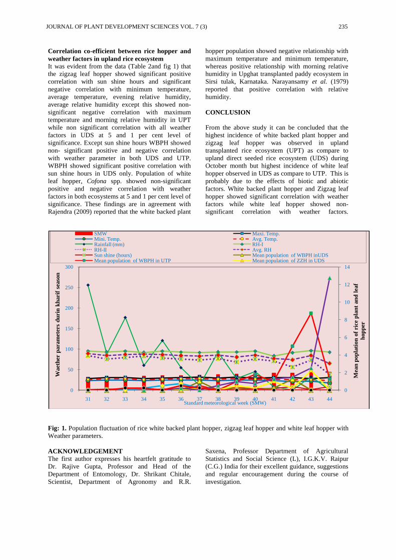
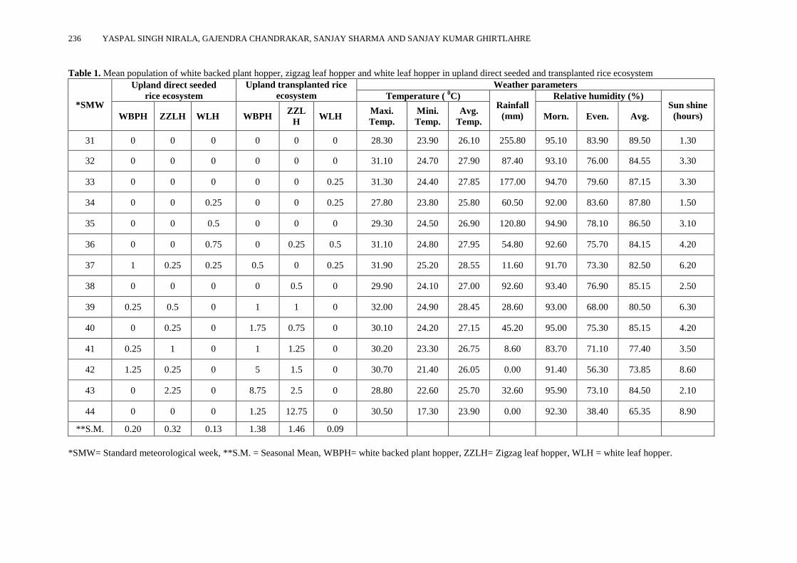
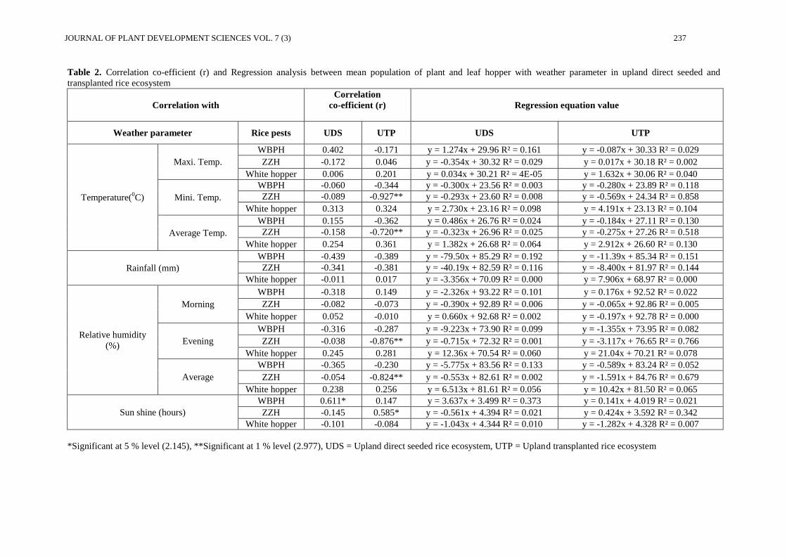
Incidence of white backed plant hopper, Sogatella furcifera (Horvath), zigzag leaf hopper, Recilia dorsalis and

white leaf hopper, Cofana spp. under upland rice ecosystem and their correlation with weather parameters

—Yaspal Singh Nirala, Gajendra Chandrakar, Sanjay Sharma and Sanjay Kumar Ghirtlahre ---- 233-238

Evaluation of efficacy of some novel chemical insecticides against stem borer, Chilo partellus (Swinhoe) in

maize

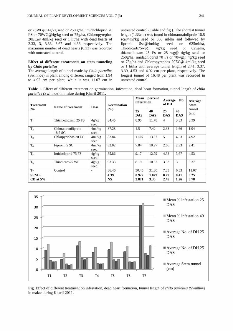
—Pradeep Kumar, Gaje Singh, Rohit Rana and Mange Ram ------------------------------------------------ 239-242

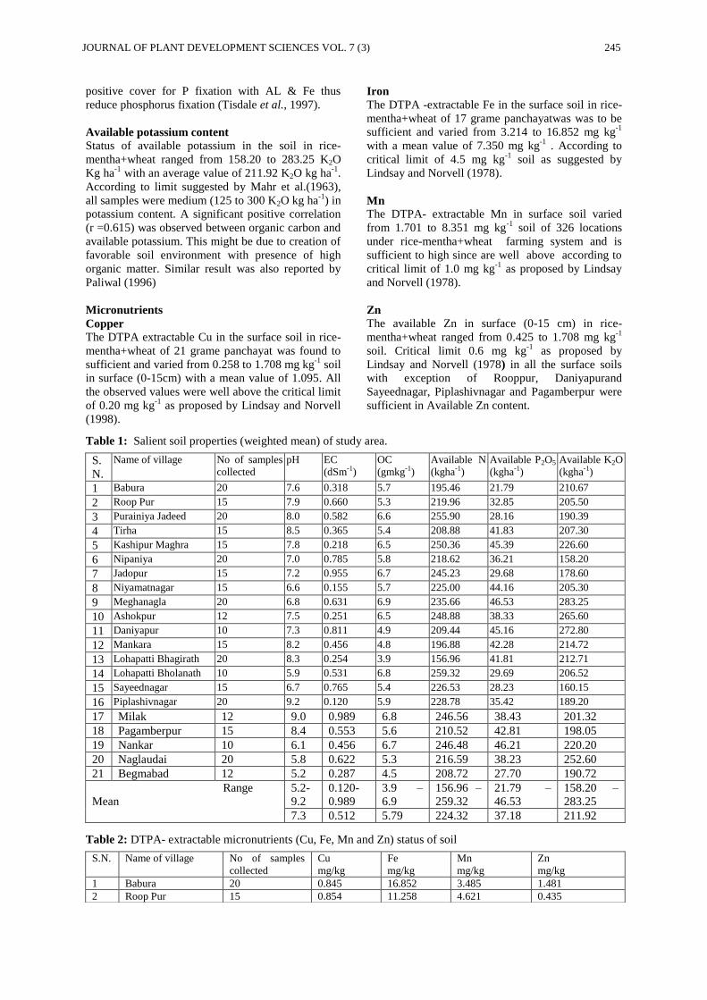
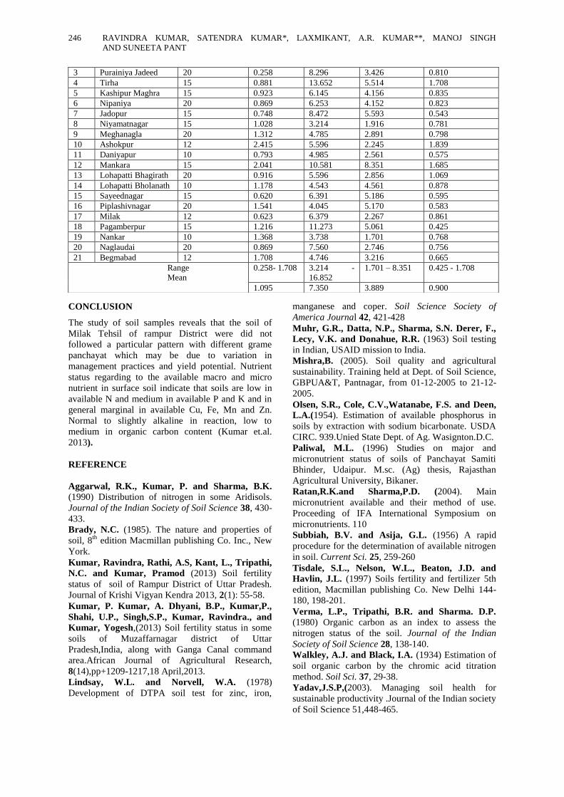
Soil quality assessment of Milak tahsil, district Rampur (Uttar Pradesh) under rice -mentha+wheat farming

system

—Ravindra Kumar, Satendra Kumar, Laxmikant, A.R. Kumar, Manoj Singh ------------------------- 243-246

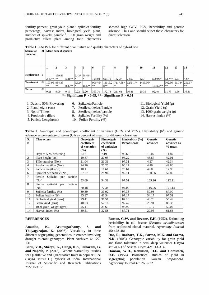
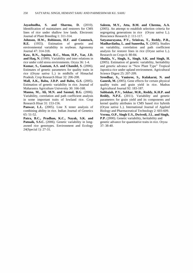
Variability and genetic parameters for grain yield in cms based rice hybrid (Oryza sativa L.)

—Satyapal Singh, Hemant Sahu and Parmeshwar Ku. Sahu ------------------------------------------------- 247-250

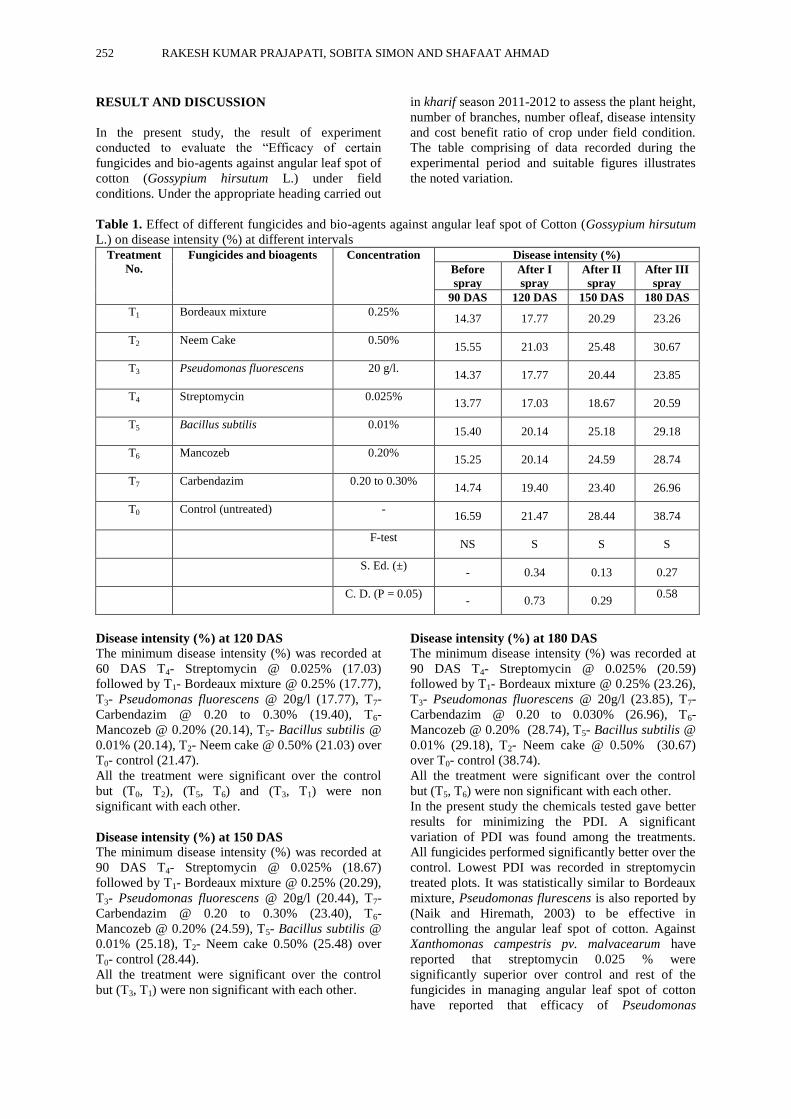
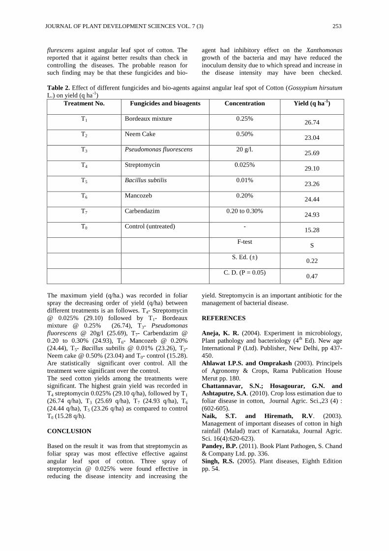
Efficacy of certain fungicides and bioagents against angular leaf spot of cotton (Gossypium hirsutum L.) under

field conditions

—Rakesh Kumar Prajapati, Sobita Simon and Shafaat Ahmad --------------------------------------------- 251-253

SHORT COMMUNICATION

Growth and energetics of rice as influenced by planting geometries and seedling densities under SRI based

cultivation practices

—Damini Thawait, Sanjay K. Dwivedi, Srishti Pandey and Kamla Gandharv --------------------------- 255-258

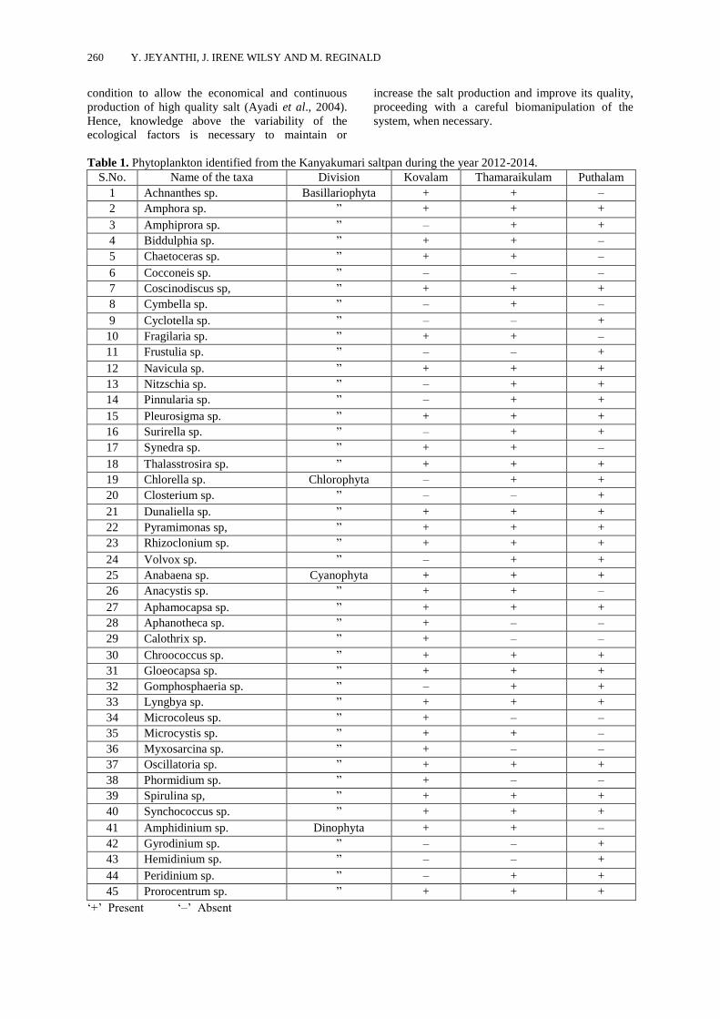
Phytoplankton assemblage in the solar saltpans of Kanyakumari district, Tamil Nadu

—Y. Jeyanthi, J. Irene Wilsy and M. Reginald ------------------------------------------------------------------- 259-261

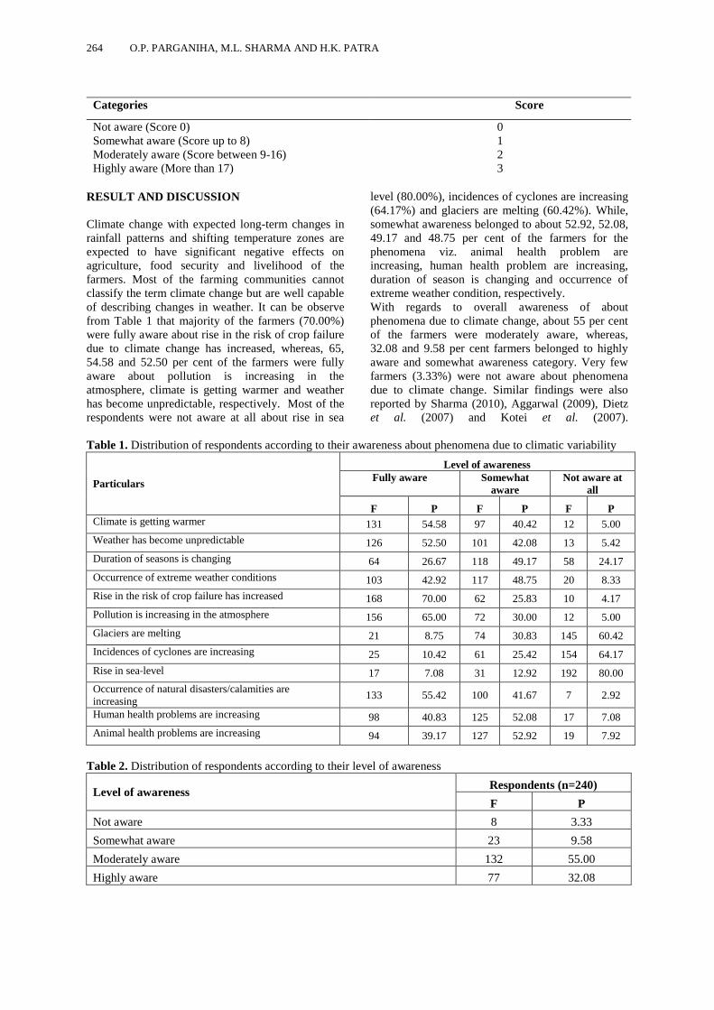
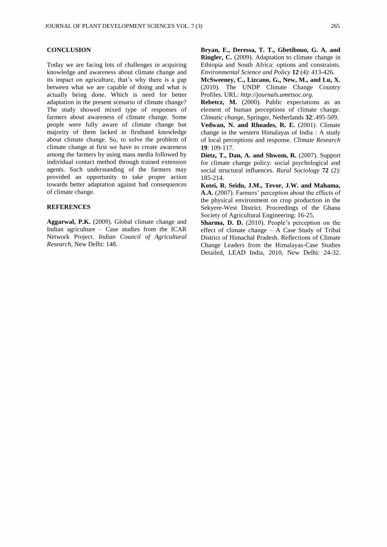
Awareness of farmers about climate change in plain zone of Chhattisgarh

—O.P. Parganiha, M.L. Sharma and H.K. Patra ----------------------------------------------------------------- 263-265

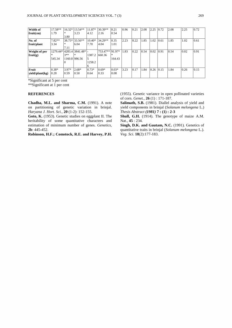
Genetic analysis of yield and its contributing traits in Brinjal (Solanum melongena L.)

—Muktar Ahmad and Manoj Kumar Singh ---------------------------------------------------------------------- 267-269

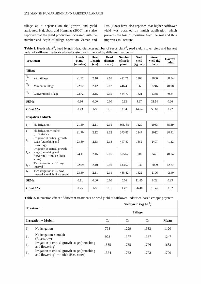
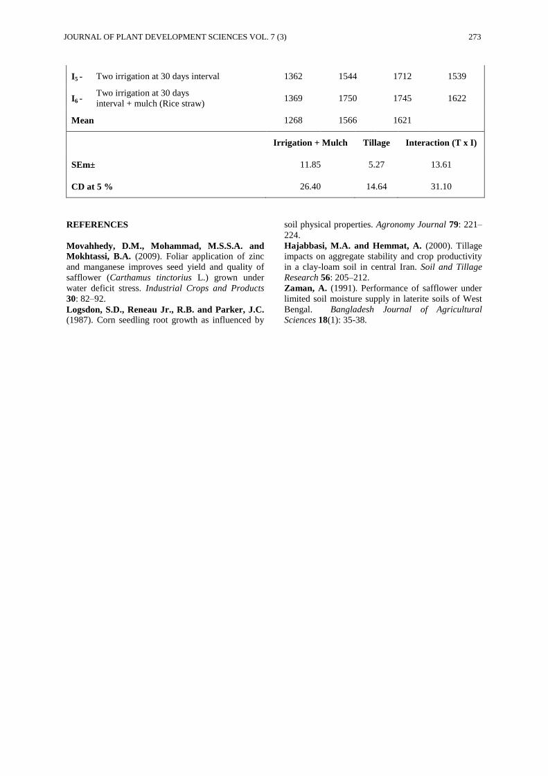
Yield attributing characters and yield of safflower under rice based cropping system

—Manish Kumar Singh and Rajendra Lakpale ------------------------------------------------------------------ 271-273

Effect of crop geometry and weed management practices on growth and productivity of Soybean

—Hemkanti Purena, Rajendra Lakpale and Chandrasekhar ------------------------------------------------- 275-278

ii

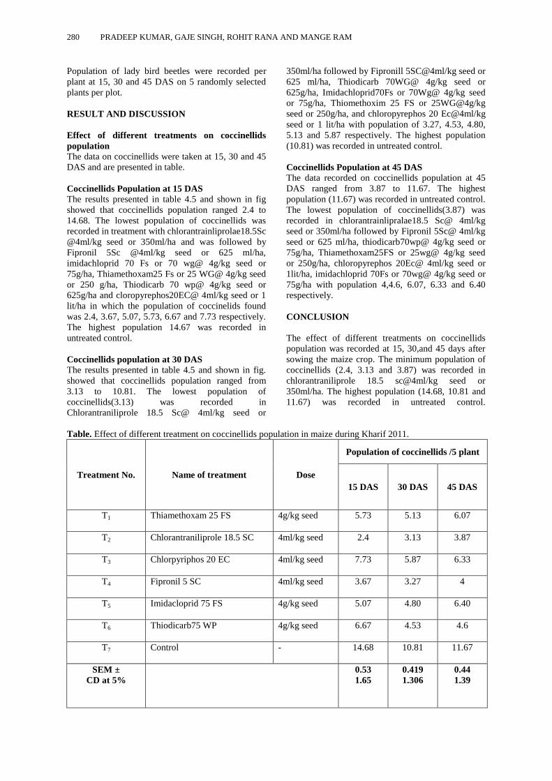
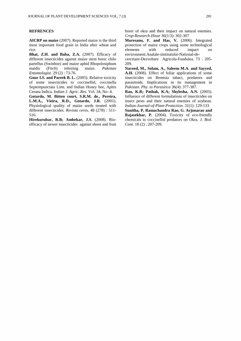
Evaluate the efficacy of some novel chemical insecticides on natural enemies in Maize

—Pradeep Kumar, Gaje Singh, Rohit Rana and Mange Ram ------------------------------------------------ 279-281

Assessment of copping mechanism of farmers to mitigate disaster due to climate change in Chhattisgarh plain

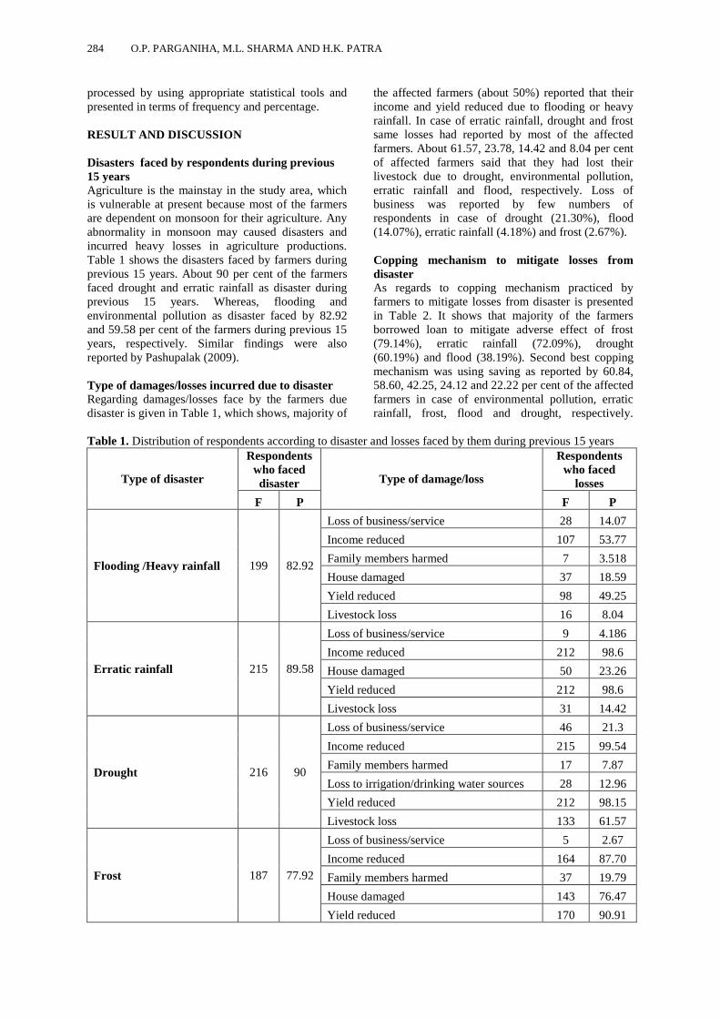
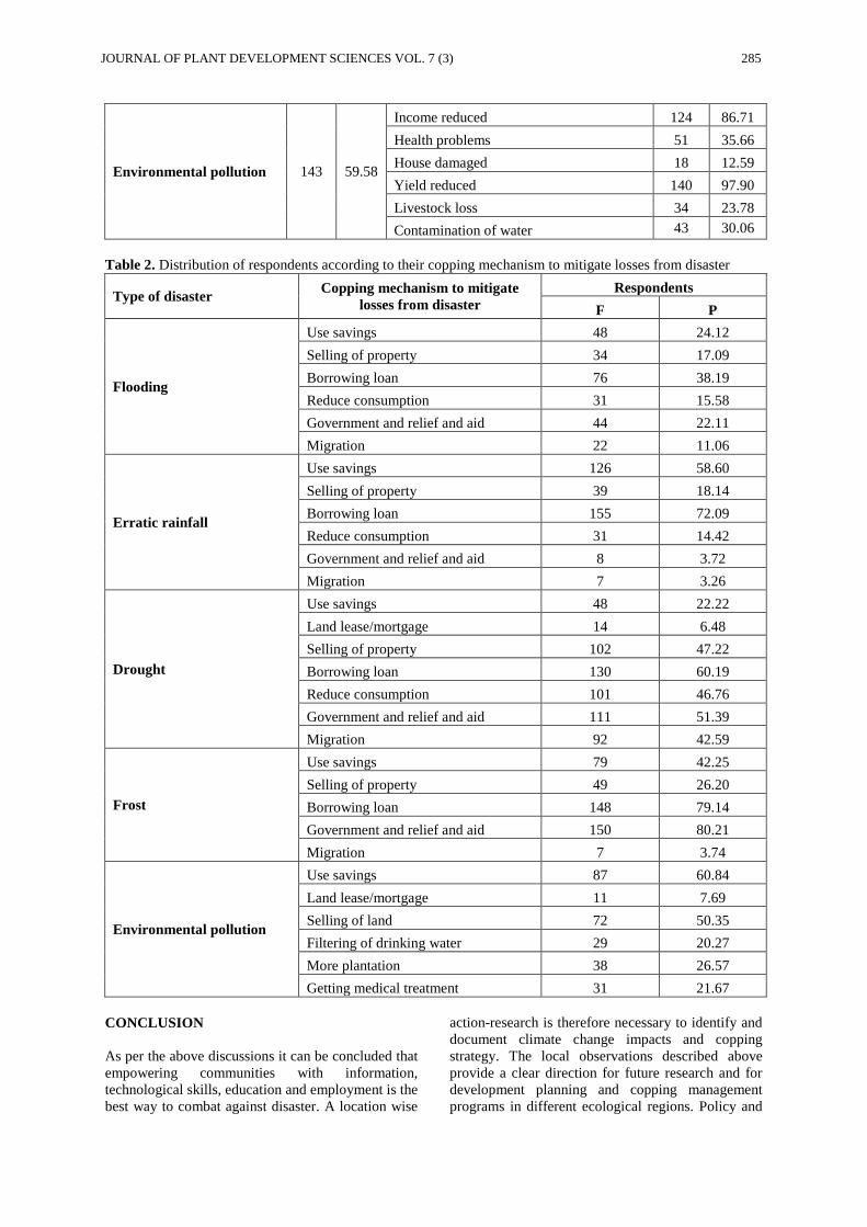
—O.P. Parganiha, M.L. Sharma and H.K. Patra ----------------------------------------------------------------- 283-286

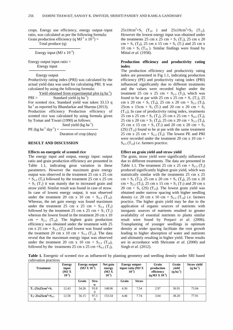
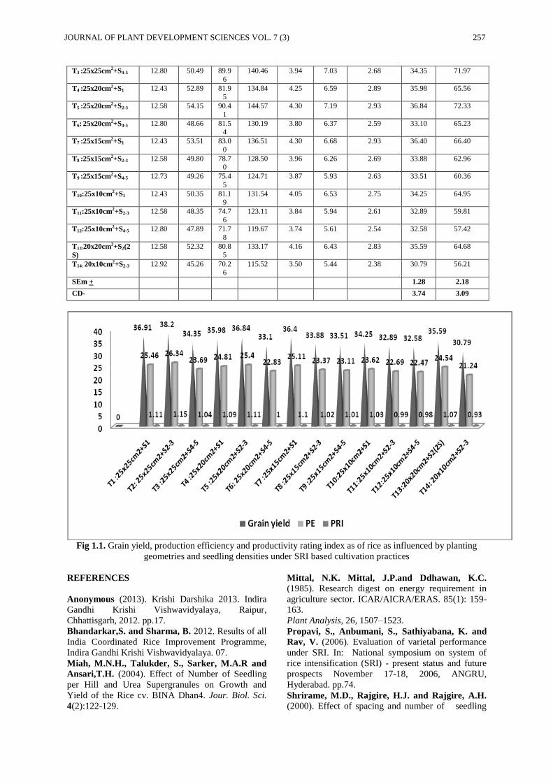
Effect of planting geometry and seedling densities on light interception in rice cultivation

—Damini Thawait, S.K. Dwivedi, Srishti Pandey and Manish Kumar Sharma -------------------------- 287-288

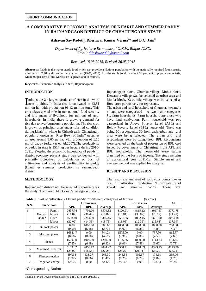
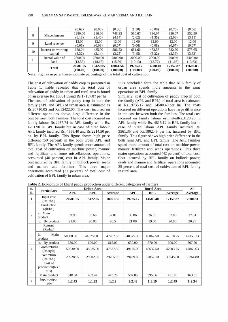
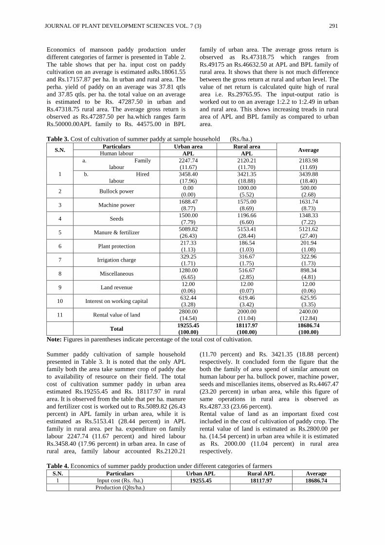
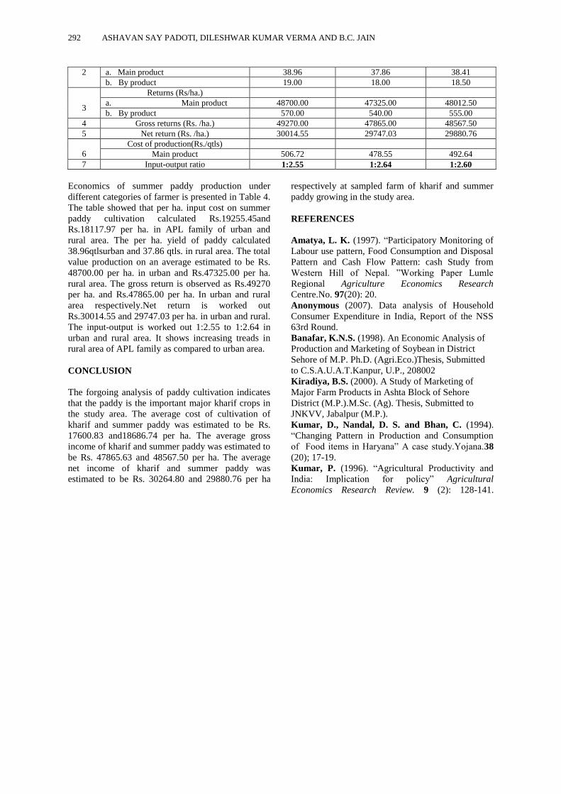
A comparative economic analysis of Kharif and summer paddy in Rajnandgaon district of Chhattisgarh state

—Ashavan Say Padoti, Dileshwar Kumar Verma and B.C. Jain --------------------------------------------- 289-292

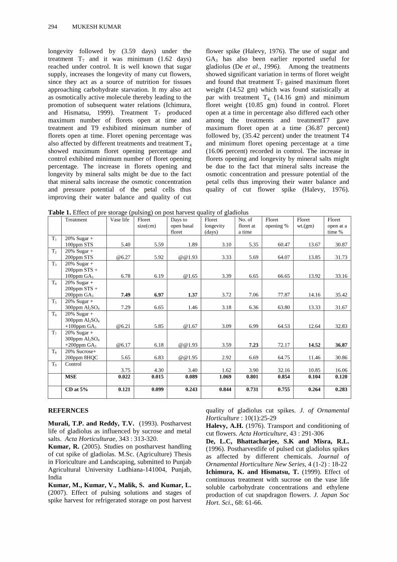
Effect of pulsing with chemicals on post-harvest quality of gladiolus (Gladiolus hybridus hort.) cv. peater pears

—Mukesh Kumar -------------------------------------------------------------------------------------------------------- 293-294

*Corresponding Author

________________________________________________ Journal of Plant Development Sciences Vol. 7 (3) : 209-216. 2015

INVENTORYING AND MONITORING OF AQUATIC PLANT DIVERSITY OF

FLUVIAL ECOSYSTEM OF RAJAJI NATIONAL PARK, UTTARAKHAND, INDIA

Nusrat Samweel* and Tahir Nazir

Department of Forestry,Dolphin (PG) Institute of Bio-Medical and Natural Sciences,

Mandhuwala, Dehradun, India

Received-10.02.2015, Revised-21.02.2015 Abstract : Aquatic plant diversity and the physico-chemical characteristics of the aquatic habitat of Song and Suswa river

flowing in the Rajaji National Park, Uttarankhand, has been monitored seasonally. Four sampling sites S1, S2, S3 and S4 were

identified. S1 and S2, at Song river S3 and S4 at Suswa river of Rajaji National Park. Seasonal sampling was done and the

study revealed that diversity has been found to be high in winter months comparatively due to low turbidity, high water

transparency, high dissolved oxygen and low water velocity

Keywords: Inventoring, Monitoring, Physico-chemical parameters, Aquatic, Habitats, Rajaji National Park

INTRODUCTION

iodiversity or biological diversity encompasses

all species of plants, animals and micro-

organisms and the ecosystems and ecological

processes of which they are parts. It is an umbrella

term for the degree of nature‟s variety including both

the number and frequency of ecosystems, species or

genes in a given assemblage. Human survival depends

on biodiversity, not only for food, fibre and health but

also for recreation. yet human activities particularly

for the last two decades, have led to extinction of

many spacio-temporal variations in biodiversity and

relationship of biodiversity with ecosystem stability

and resilience have been the subject of concern of

ecologists for some time now (Odum,1971). Aquatic

biodiversity has been recognised as one of the most

potential and essential characteristics of life for

proper functioning of fluvial ecosystem and as a

means for coping with natural and anthropogenic

environmental changes. Aquatic biodiversity reflects

the conditions existing in the environment and

estimates the biological monitoring of water pollution

level. For ascertaining the biological status of the

river, the qualitative and quantitative investigations of

trophic levels including Phytoplankton and Periphytic

biota are important.The contribution on aquatic plant

diversity of freshwater ecosystems have been made

by Berner 1951; Schmitz 1954 1961; Douglas 1958;

Mc Conell and Singler 1959; Whitford 1960;

Grezenda et al. 1960; Holden and Green 1960;

Woods 1965; Williams 1966; Golterman et al. 1969;

Hynes 1971; Whitton 1975; Crayton and Summerfield

1979; Sze 1981; Stevenson 1984, 1996; Biggs and

Close 1989; Allan and Flecker, 1993; Biggs 1995,

1996, 1998; Biggs and Thompson 1995; Biggs and

Gerbeaux 1993; Benson-Evans et al 1975; Haury

1996; Allan 1997; Quinn et al. 1997; Clausen and

Biggs 2000; Biggs et al. 1998; Pollock et al. 1998;

Horner et al.1990; Biggs, 1996, Clausen and Biggs

1999; Iida and Ladona 2000, Smith et al. 2000;

Walsh et al. 2001, Rojo et al. 2002; Hankinson and

Blanch 2003; Harrison et al. 2004 and Sharma 2002,

2005).

Study Sites

Rajaji National Park is situated in the foothills of

Shiwalik Range of the newly carved out state

Uttarakhand. It is the part of the Dehradun, Hardwar

and Pauri district of Uttarakhand.

Three sanctuaries, Motichur Sanctuary (59.5sq.km),

Rajaji Sanctuary (247.0sq.km), Chila Sanctuary

(249.02sq.km) and other reserve forests (234.5sq.km)

are amalgamated into large protected area which is

named as Rajaji National Park. The total area of the

Rajaji National Park is 820.42km2. To the north of the

Rajaji National Park lies the Dehradun and Tehri

Forest Division. River Suswa forms the northern

natural boundary upto Ganges.

River Ganges divides the Park into two units, the

Chila Sanctuary complex in the east and Rajaji

Motichur Sanctuary Complex in the west. To the

south of Rajaji lies the revenue lands and villages of

Haridwar District. Part of south eastern portion is

covered by Bijnore forest division. The Garhwal

forest division lies to the east of the park. Rawsan

river forms a small portion of natural south eastern

boundary of the park. To the west of the Rajaji lies

the Shiwalik Forest Division. Song and Suswa are

two perennial rivers draining Rajaji National Park in

north eastern slopes of Shiwalik. The north eastern

slopes of Shiwaliks are very steep and rugged in the

upper portion but in the lower portion it has a quiet

easy gradient. There are large number of short,

shallow dry and bouldery streams locally known as

“raus”coming down from upper slopes and carring

their discharge into Song and Suswa rivers. The forest

on both the sides of the Suswa river is more or less on

flat or gently sloping area often cut by nalas. The

forests of eastern Doon are drained by Suswa and

Song rivers. River Song and Suswa form its

confluence in the Banbaha forest block. From there, it

flows in a south eastern direction till it discharges into

the Ganges near Satyanarian. Some seasonal

B

210 NUSRAT SAMWEEL AND TAHIR NAZIR

tributaries also meet Song and Suswa river at Bindal,

Rispana, Ren and Jakhan The river Suswa flows very

nearly opposite to Asan river to the east of

Saharanpur-Mussoorie highway and flows in a south

easterly direction to discharge into the Song. After a

preliminary survey of Song and Suswa river, four

sampling sites (S1, S2, S3 and S4) were selected. S1

and S2 were identified at Song river and S3 and S4

were identified at the Suswa river. Site S1 was

selected at Shampur, S2 at Chidderwala, S3 at

Satyanarian and S4 at Kansrao.

Considerable work has been done on the teresstrial

biodiversity of Rajaji National Park (Diwakar; 1995,

Panwar and Mishra; 1994), but less information is

available so far on the aquatic plant diversity and the

function of fluvial ecosystem of Rajaji National Park.

Therefore the present work on the inventoring and

monitoring of aquatic plant diversity of the river Song

and Suswa of Rajaji National Park was carried out.

MATERIAL AND METHOD

Sampling was conducted seasonally winter

(November-February), Summer (March-June) and

Monsoon (July-October). Air and Water temperature

was recorded with the help of a Centigrade 0-110 0C

thermometer. The mean velocity was measured using

electromagnetic current meter (model-PVM-2A). pH

was estimated by control dynamics pH meter (model-

APX15\C) while turbidity was measured by turbidity

meter (model-5D1M). Nitrates and phosphates were

estimated by the spectrophotometer (Spectronic 20D

Series) and sodium and potassium were estimated by

the digital flame photometer (model-1381). Dissolved

oxygen and Free CO2 were measured following

methods outlined in APHA (1998). The control

dynamics conductivity meter (model-API 185) was

used for measuring conductivity. All these parameters

were determined following the standard methods

outlined in Welch (1952), APHA (1998) and Wetzel

and Likens (1992). Some of the physico-chemical

parameters were analised at the spot and rest were

determined at the laboratory. For the analysis of

biological parameters, the samples of periphyton were

preserved in 4% formalin for quantitative study, while

phytoplankton was preserved in Lugol‟s solution and

3% formalin, respectively. The quantitative analysis

was made by using Ward and Whipple (1992) and

several taxonomic keys and manuals of Freshwater

Biological Association, UK.

The percentage cover of different sized substrata

within each surber quadrate was estimated visually

using the substrate size classes (after Bovee and

Milhous 1978) of sand (0.06-2mm), fine gravel (2-

32mm), coarse gravel (32-64mm), cobbles (64-

256mm) and boulders (>256mm) with Surber

Sampler (0.5mm mesh net) to a depth about 10cm in a

quadrat. Samples were preserved in 4% formalin.

RESULT AND DISCUSSION

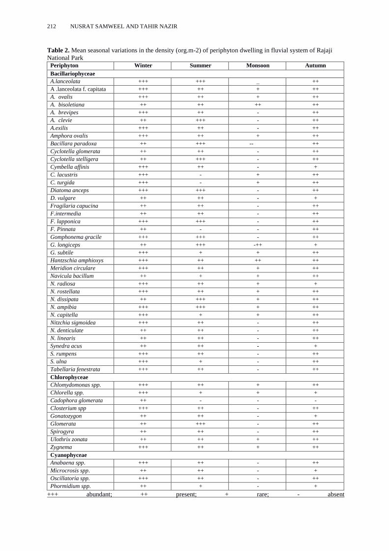
Periphytons (attached algae) are also the dominant

primary producers in the fluvial system of Rajaji

National Park. A total of 51 genera of periphyton

were recorded from the fluvial ecosystem of Rajaji

National park. Periphyton were represented by

Bacillariophyceae (38 genera), Chlorophyceae (9

genera) and Myxophyceae (4 genera) Table2.

Periphyton community showed maximum abundance

during winter season and minimum during monsoon

season. Maximum periphytonic biomass was

observed in Danish lowland streams during spring

season (Sand Jenson et al. 1988). Gusain (1991)

recorded maximum periphyton biomass during winter

in Bhilangana river, Garhwal Himalayas. While

Shamsudin and Sleigh (1994) recorded maximum

periphyton biomass during spring season in Chalk

stream and soft water stream. Moore (1997) and

Morin (2004) recorded an increase in periphytic

biomass in sub-arctic streams during summers when

low temperature was recorded. For temperate streams,

Cox (1990) recorded a minimum biomass in winter,

with a spring maxima, followed by unpredictable

fluctuations in biomass during summer.

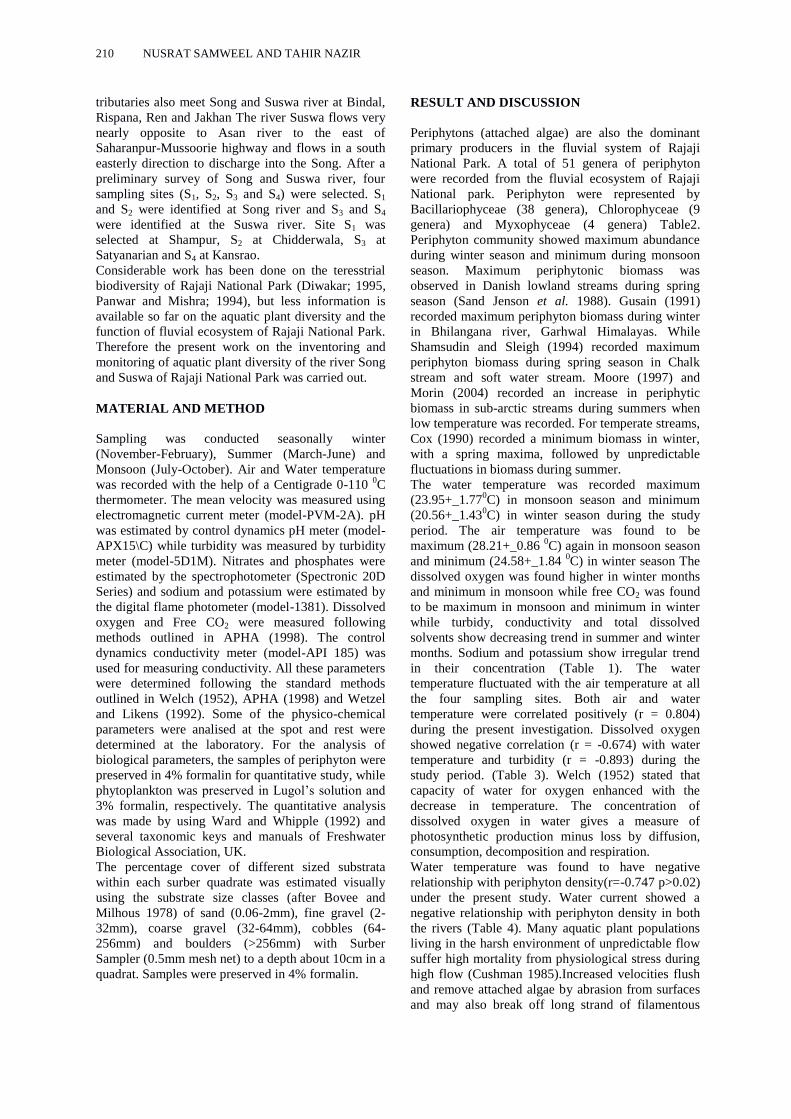
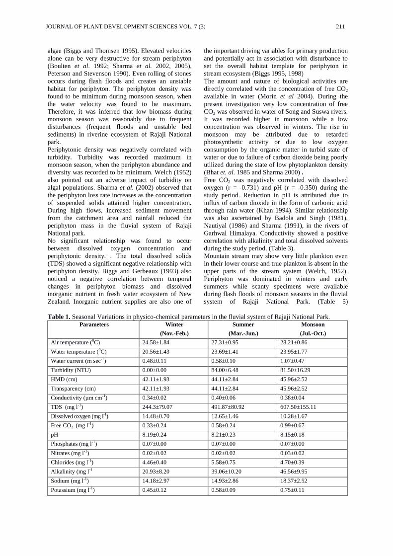
The water temperature was recorded maximum

(23.95+_1.770C) in monsoon season and minimum

(20.56+_1.430C) in winter season during the study

period. The air temperature was found to be

maximum (28.21+_0.86 0C) again in monsoon season

and minimum (24.58+_1.84 0C) in winter season The

dissolved oxygen was found higher in winter months

and minimum in monsoon while free CO2 was found

to be maximum in monsoon and minimum in winter

while turbidy, conductivity and total dissolved

solvents show decreasing trend in summer and winter

months. Sodium and potassium show irregular trend

in their concentration (Table 1). The water

temperature fluctuated with the air temperature at all

the four sampling sites. Both air and water

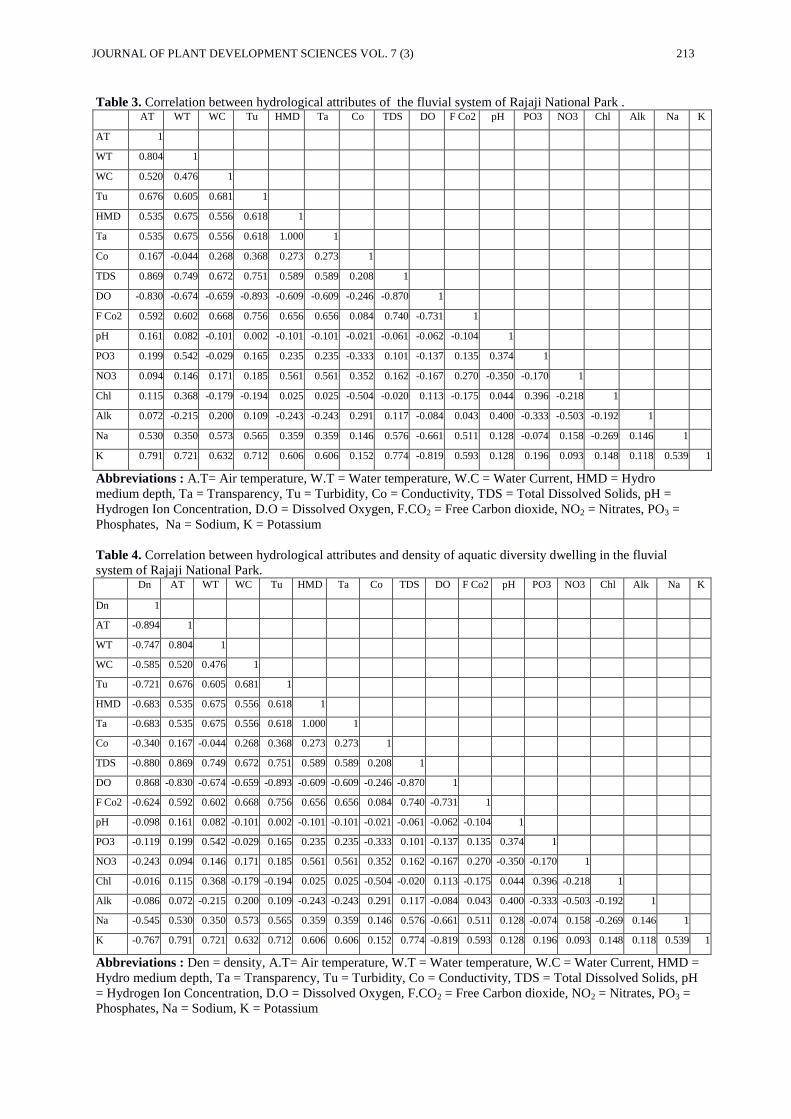
temperature were correlated positively (r = 0.804)

during the present investigation. Dissolved oxygen

showed negative correlation (r = -0.674) with water

temperature and turbidity (r = -0.893) during the

study period. (Table 3). Welch (1952) stated that

capacity of water for oxygen enhanced with the

decrease in temperature. The concentration of

dissolved oxygen in water gives a measure of

photosynthetic production minus loss by diffusion,

consumption, decomposition and respiration.

Water temperature was found to have negative

relationship with periphyton density(r=-0.747 p>0.02)

under the present study. Water current showed a

negative relationship with periphyton density in both

the rivers (Table 4). Many aquatic plant populations

living in the harsh environment of unpredictable flow

suffer high mortality from physiological stress during

high flow (Cushman 1985).Increased velocities flush

and remove attached algae by abrasion from surfaces

and may also break off long strand of filamentous

JOURNAL OF PLANT DEVELOPMENT SCIENCES VOL. 7 (3) 211

algae (Biggs and Thomsen 1995). Elevated velocities

alone can be very destructive for stream periphyton

(Boulten et al. 1992; Sharma et al. 2002, 2005),

Peterson and Stevenson 1990). Even rolling of stones

occurs during flash floods and creates an unstable

habitat for periphyton. The periphyton density was

found to be minimum during monsoon season, when

the water velocity was found to be maximum.

Therefore, it was inferred that low biomass during

monsoon season was reasonably due to frequent

disturbances (frequent floods and unstable bed

sediments) in riverine ecosystem of Rajaji National

park.

Periphytonic density was negatively correlated with

turbidity. Turbidity was recorded maximum in

monsoon season, when the periphyton abundance and

diversity was recorded to be minimum. Welch (1952)

also pointed out an adverse impact of turbidity on

algal populations. Sharma et al. (2002) observed that

the periphyton loss rate increases as the concentration

of suspended solids attained higher concentration.

During high flows, increased sediment movement

from the catchment area and rainfall reduced the

periphyton mass in the fluvial system of Rajaji

National park.

No significant relationship was found to occur

between dissolved oxygen concentration and

periphytonic density. . The total dissolved solids

(TDS) showed a significant negative relationship with

periphyton density. Biggs and Gerbeaux (1993) also

noticed a negative correlation between temporal

changes in periphyton biomass and dissolved

inorganic nutrient in fresh water ecosystem of New

Zealand. Inorganic nutrient supplies are also one of

the important driving variables for primary production

and potentially act in association with disturbance to

set the overall habitat template for periphyton in

stream ecosystem (Biggs 1995, 1998)

The amount and nature of biological activities are

directly correlated with the concentration of free CO2

available in water (Morin et al 2004). During the

present investigation very low concentration of free

CO2 was observed in water of Song and Suswa rivers.

It was recorded higher in monsoon while a low

concentration was observed in winters. The rise in

monsoon may be attributed due to retarded

photosynthetic activity or due to low oxygen

consumption by the organic matter in turbid state of

water or due to failure of carbon dioxide being poorly

utilized during the state of low phytoplankton density

(Bhat et. al. 1985 and Sharma 2000) .

Free CO2 was negatively correlated with dissolved

oxygen (r = -0.731) and pH (r = -0.350) during the

study period. Reduction in pH is attributed due to

influx of carbon dioxide in the form of carbonic acid

through rain water (Khan 1994). Similar relationship

was also ascertained by Badola and Singh (1981),

Nautiyal (1986) and Sharma (1991), in the rivers of

Garhwal Himalaya. Conductivity showed a positive

correlation with alkalinity and total dissolved solvents

during the study period. (Table 3).

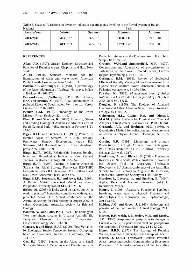
Mountain stream may show very little plankton even

in their lower course and true plankton is absent in the

upper parts of the stream system (Welch, 1952).

Periphyton was dominated in winters and early

summers while scanty specimens were available

during flash floods of monsoon seasons in the fluvial

system of Rajaji National Park. (Table 5)

Table 1. Seasonal Variations in physico-chemical parameters in the fluvial system of Rajaji National Park.

Parameters Winter

(Nov.-Feb.)

Summer

(Mar.-Jun.)

Monsoon

(Jul.-Oct.)

Air temperature (0C) 24.58±1.84 27.31±0.95 28.21±0.86

Water temperature (0C) 20.56±1.43 23.69±1.41 23.95±1.77

Water current (m sec-1) 0.48±0.11 0.58±0.10 1.07±0.47

Turbidity (NTU) 0.00±0.00 84.00±6.48 81.50±16.29

HMD (cm) 42.11±1.93 44.11±2.84 45.96±2.52

Transparency (cm) 42.11±1.93 44.11±2.84 45.96±2.52

Conductivity (µm cm-1) 0.34±0.02 0.40±0.06 0.38±0.04

TDS (mg l-1) 244.3±79.07 491.87±80.92 607.50±155.11

Dissolved oxygen (mg l-1) 14.48±0.70 12.65±1.46 10.28±1.67

Free CO2 (mg l-1) 0.33±0.24 0.58±0.24 0.99±0.67

pH 8.19±0.24 8.21±0.23 8.15±0.18

Phosphates (mg l-1) 0.07±0.00 0.07±0.00 0.07±0.00

Nitrates (mg l-1) 0.02±0.02 0.02±0.02 0.03±0.02

Chlorides (mg l-1) 4.46±0.40 5.58±0.75 4.70±0.39

Alkalinity (mg l-1 20.93±8.20 39.06±10.20 46.56±9.95

Sodium (mg l-1) 14.18±2.97 14.93±2.86 18.37±2.52

Potassium (mg l-1) 0.45±0.12 0.58±0.09 0.75±0.11


Table 2. Mean seasonal variations in the density (org.m-2) of periphyton dwelling in fluvial system of Rajaji

National Park Periphyton Winter Summer Monsoon Autumn

Bacillariophyceae

A.lanceolata +++ +++ _ ++

A .lanceolata f. capitata +++ ++ + ++

A. ovalis +++ ++ + ++

A. bisoletiana ++ ++ ++ ++

A. brevipes +++ ++ - ++

A. clevie ++ +++ - ++

A.exilis +++ ++ - ++

Amphora ovalis +++ ++ + ++

Bacillara paradoxa ++ +++ -- ++

Cyclotella glomerata ++ ++ - ++

Cyclotella stelligera ++ +++ - ++

Cymbella affinis +++ ++ - +

C. lacustris +++ - + ++

C. turgida +++ - + ++

Diatoma anceps +++ +++ - ++

D. vulgare ++ ++ - +

Fragilaria capucina ++ ++ - ++

F.intermedia ++ ++ - ++

F. lapponica +++ +++ - ++

F. Pinnata ++ - - ++

Gomphonema gracile +++ +++ - ++

G. longiceps ++ +++ -++ +

G. subtile +++ + + ++

Hantzschia amphioxys +++ ++ ++ ++

Meridion circulare +++ ++ + ++

Navicula bacillum ++ + + ++

N. radiosa +++ ++ + +

N. rostellata +++ ++ + ++

N. dissipata ++ +++ + ++

N. ampibia +++ +++ + ++

N. capitella +++ + + ++

Nitzchia sigmoidea +++ ++ - ++

N. denticulate ++ ++ - ++

N. linearis ++ ++ - ++

Synedra acus ++ ++ - +

S. rumpens +++ ++ - ++

S. ulna +++ + - ++

Tabellaria fenestrata +++ ++ - ++

Chlorophyceae

Chlomydomonas spp. +++ ++ + ++

Chlorella spp. +++ + + +

Cadophora glomerata ++ - - -

Closterium spp +++ ++ - ++

Gonatozygon ++ ++ - +

Glomerata ++ +++ - ++

Spirogyra ++ ++ - ++

Ulothrix zonata ++ ++ + ++

Zygnema +++ ++ + ++

Cyanophyceae

Anabaena spp. +++ ++ - ++

Microcrosis spp. ++ ++ - +

Oscillatoria spp. +++ ++ - ++

Phormidium spp. ++ + - +

+++ abundant; ++ present; + rare; - absent


Table 3. Correlation between hydrological attributes of the fluvial system of Rajaji National Park . AT WT WC Tu HMD Ta Co TDS DO F Co2 pH PO3 NO3 Chl Alk Na K

AT 1

WT 0.804 1

WC 0.520 0.476 1

Tu 0.676 0.605 0.681 1

HMD 0.535 0.675 0.556 0.618 1

Ta 0.535 0.675 0.556 0.618 1.000 1

Co 0.167 -0.044 0.268 0.368 0.273 0.273 1

TDS 0.869 0.749 0.672 0.751 0.589 0.589 0.208 1

DO -0.830 -0.674 -0.659 -0.893 -0.609 -0.609 -0.246 -0.870 1

F Co2 0.592 0.602 0.668 0.756 0.656 0.656 0.084 0.740 -0.731 1

pH 0.161 0.082 -0.101 0.002 -0.101 -0.101 -0.021 -0.061 -0.062 -0.104 1

PO3 0.199 0.542 -0.029 0.165 0.235 0.235 -0.333 0.101 -0.137 0.135 0.374 1

NO3 0.094 0.146 0.171 0.185 0.561 0.561 0.352 0.162 -0.167 0.270 -0.350 -0.170 1

Chl 0.115 0.368 -0.179 -0.194 0.025 0.025 -0.504 -0.020 0.113 -0.175 0.044 0.396 -0.218 1

Alk 0.072 -0.215 0.200 0.109 -0.243 -0.243 0.291 0.117 -0.084 0.043 0.400 -0.333 -0.503 -0.192 1

Na 0.530 0.350 0.573 0.565 0.359 0.359 0.146 0.576 -0.661 0.511 0.128 -0.074 0.158 -0.269 0.146 1

K 0.791 0.721 0.632 0.712 0.606 0.606 0.152 0.774 -0.819 0.593 0.128 0.196 0.093 0.148 0.118 0.539 1

Abbreviations : A.T= Air temperature, W.T = Water temperature, W.C = Water Current, HMD = Hydro

medium depth, Ta = Transparency, Tu = Turbidity, Co = Conductivity, TDS = Total Dissolved Solids, pH =

Hydrogen Ion Concentration, D.O = Dissolved Oxygen, F.CO2 = Free Carbon dioxide, NO2 = Nitrates, PO3 =

Phosphates, Na = Sodium, K = Potassium

Table 4. Correlation between hydrological attributes and density of aquatic diversity dwelling in the fluvial

system of Rajaji National Park. Dn AT WT WC Tu HMD Ta Co TDS DO F Co2 pH PO3 NO3 Chl Alk Na K

Dn 1

AT -0.894 1

WT -0.747 0.804 1

WC -0.585 0.520 0.476 1

Tu -0.721 0.676 0.605 0.681 1

HMD -0.683 0.535 0.675 0.556 0.618 1

Ta -0.683 0.535 0.675 0.556 0.618 1.000 1

Co -0.340 0.167 -0.044 0.268 0.368 0.273 0.273 1

TDS -0.880 0.869 0.749 0.672 0.751 0.589 0.589 0.208 1

DO 0.868 -0.830 -0.674 -0.659 -0.893 -0.609 -0.609 -0.246 -0.870 1

F Co2 -0.624 0.592 0.602 0.668 0.756 0.656 0.656 0.084 0.740 -0.731 1

pH -0.098 0.161 0.082 -0.101 0.002 -0.101 -0.101 -0.021 -0.061 -0.062 -0.104 1

PO3 -0.119 0.199 0.542 -0.029 0.165 0.235 0.235 -0.333 0.101 -0.137 0.135 0.374 1

NO3 -0.243 0.094 0.146 0.171 0.185 0.561 0.561 0.352 0.162 -0.167 0.270 -0.350 -0.170 1

Chl -0.016 0.115 0.368 -0.179 -0.194 0.025 0.025 -0.504 -0.020 0.113 -0.175 0.044 0.396 -0.218 1

Alk -0.086 0.072 -0.215 0.200 0.109 -0.243 -0.243 0.291 0.117 -0.084 0.043 0.400 -0.333 -0.503 -0.192 1

Na -0.545 0.530 0.350 0.573 0.565 0.359 0.359 0.146 0.576 -0.661 0.511 0.128 -0.074 0.158 -0.269 0.146 1

K -0.767 0.791 0.721 0.632 0.712 0.606 0.606 0.152 0.774 -0.819 0.593 0.128 0.196 0.093 0.148 0.118 0.539 1

Abbreviations : Den = density, A.T= Air temperature, W.T = Water temperature, W.C = Water Current, HMD =

Hydro medium depth, Ta = Transparency, Tu = Turbidity, Co = Conductivity, TDS = Total Dissolved Solids, pH

= Hydrogen Ion Concentration, D.O = Dissolved Oxygen, F.CO2 = Free Carbon dioxide, NO2 = Nitrates, PO3 =

Phosphates, Na = Sodium, K = Potassium


Table 5. Seasonal Variations in diversity indices of aquatic plants dwelling in the fluvial system of Rajaji

National Park

Season/Year Winter Summer Monsoon Autumn

2001-2002 3.495±0.15 3.375±0.13 3.088±0.08 3.247±0.04

2002-2003 3.613±0.17 3.485±0.17 3.203±0.40 3.288±0.05

REFERENCES

Allan, J.D. (1997). Stream Ecology: Structure and

Function of Running waters. Chapman and Hall, New

York.

APHA (1998). Standard Methods for the

Examination of water and waste water. American

Public Health Association. New York, USA.

Badola, S.P. and Singh, H.R. (1981). Hydrobiology

of the River Alaknanda of Garhwal Himalaya. Indian

J. Ecology, 8 : 269-276.

Bensen-Evans, E.,Williams, K.P.F. Mc Clean,

R.O. and pranne, N. (1975). Algal communities in

polluted Rivers of South wales. Ver. Internat. Verein

Limnol, 19 : 2002-2019.

Berner, L.M. (1951). Limnology of the lower

Missouri River. Ecology, 32 : 1-12.

Bhat, D. and Sharma, R. (2000). Diversity, Status

and Feeding Ecology of Avifauna in Motichur area of

Rajaji National Park, India. Annuals of Forestry 8(2):

179-141.

Biggs, B.J.F. and Gerbeaux. G. (1993). Patterns in

Benthic Algae of Streams. In : Algal ecology

Freshwater Benthic Ecosystems. (eds.) R.J.

Stevenson, M.L Bothwell and R L lowe : Academic

press, New York. 1-789.

Biggs, B.J.F. (1995). Relationship between Benthic

biota and Hydrological Indices in New Zealand

streams. Freshwater Biology, 38 : 327-342.

Biggs, B.J.F. (1996). Patterns in Benthic Algae of

Streams: In: Algal Ecology Freshwater BENTHIC

Ecosystems (eds.) R.J Stevenson, M.L Bothwell and

R.L. Lowe. Academic Press, New York.

Biggs B.J.F., Stevenson, R.J and lowe, R.L. (1998).

A Habitat Matrix conceptual Model for stream

Periphyton. Fresh Hydrobiol 143 (I) : 21-56.

Bishop, M. (2003). It looks Good on paper, but will it

work in practice? Improving compliance with aquatic

protected Areas. 31st Annual conference of the

Australian society for Fish biology in August 2002 in

cairns, Queensland. Australian society for fish and

Biology.

Boulton, A.J.and Lake, P.S. (1992). The Ecology of

Two intermittent streams in Victoria Australia III.

Temporal Changes in Faunal Composition.

Freshwater Biology, 27 : 123-138.

Clausen, B and Biggs, B.J.F. (2000). Flow Variables

for Ecological Studies Temperate Streams: Groupings

based on Covariance. Journal of Hydrology, 237 :

184-197.

Cox, E.J. (1990). Studies on the Algae of a Small

Soft water Stream.I. Occurrence and Distribution with

Particular reference to the Diatoms. Arch. Hydrobiol.

Suppl., 83 : 525-552.

Crayton, W.M.and Summerfield, M.R. (1979).

Composition and Abundance of phytoplankton in

Tributaries of the Lower Colorado River, Canyon

Region. Hyrobiologia, 61 : 81-93.

Cushman, R.M. (1985). Review of Ecological

Effects of Rapidly Varying Flows Downstream form

Hydroelectric facilities. North American Journal of

Fisheries Management, 5 : 330-339.

Diwakar K. (1995). Management plan of Rajaji

National Park, Dehradun for the period of 1995-96 to

2005-2006 Vol. I & II.

Douglas, B. (1958). The Ecology of Attached

Diatoms and Other Algae in Small Stony Streams J.

ecology, 46 : 295-322.

Golterman, H.L., Clymo, R.S. and Ohnstad,

M.A.M. (1969). Methods for Physical and Chemical

Analyses of freshwaters. Blackwell Sci. Publ. Oxford.

Grezenda, A.R. and Brehmer, M.L. (1960). A

Quantitative Method for collection and Measurement

of stream Periphyton. Limnol. Oceanogr., 5 : 190-

194.

Gusain, O.P. (1991). Limnology and primary

Productivity in a High Altitude River Bhilangana.

Ph.D. thesis submitted to H.N.B. Garhwal University

Srinagar Garhwal. 1-217.

Hankinson, A. and Blanch, S. (2003). Freshwater

Reserves in New South Wales, Australia a powerful

but Unused Tool for Conserving Freshwater

Biodiversity. 31st Annual conference of the Australian

Society for fish Biology in August 2002 in Cairns,

Queensland. Australian Society for Fish Biology.

Harrison I., Laverty, m. and Sterling, E. (2004).

Alpha, Beta and Gamma diversity. (ed.) C.

Reedstrom, Melina.

Haury, J. (1996). Assessory Functional Typology

Involving water quality, physical Freatures and

Macrophytes in a Normandy river. Hydrobiologia,

340 : 43-49.

Holden, J.M. and Green, J. (1960). Hydrology and

plankton of the river Sokoto.J .Animal Ecology, 291 :

65-84.

Horner, R.R. welch, E.B. Seeley, M.R. and Jacoby,

J.M. (1990). Responses of periphyton to changes in

Current velocity, Suspended sediment and phosphorus

Concentration. Freshwater Biology, 24 : 212-232.

Hynes, H.B.N. (1971). The Ecology of Running

Waters, Liverpool University Press Liverpool, 1-555.

Koehn, J. (2003). Freshwater Aquatic Protected

Areas- protecting species, Communities or Ecosystem

Processes. 31st Annual Conference of the Australian


Society for Fish Biology in August 2002 in Cairns,

Queensland. Australian society for fish and Biology.

Khan, R.A. (2002). Diversity of Freshwater

Macroinvertebrate Communities Associated with

Macrophytes. Rec. Zool. Soc. India, 30(1) : 79-86.

Khan, A. (2004). Elephant-habitat interaction and its

management implications in Rajaji National Park.

Ph.D.Dissertation. Aligarh Muslim University,

Aligarh.271 pp.

Koehn, J. (2003). Freshwater Aquatic Protected

Areas- protecting species, Communities or Ecosystem

Processes. 31st Annual Conference of the Australian

Society for Fish Biology in August 2002 in Cairns,

Queensland. Australian society for fish and Biology.

Lida , S. and Ladono , Y. (2000). Genetic

Biodiversity of Potamogeton Angiollanw in Lake

Biwa, Japan. Aquatic Bot. 67:100 pp

Quinn, J.M., Copper, A.B., Davies- colley R.J.

Rutherford J.C. and Williamson, R.B. (1997).

Land-use Effects on Habitat, water Quality,

Periphyton and benthic Invertebrates in Waikato,

New Zealand, hill country Streams. New Zealand

Journal of Marine and Freshwater Research, 31 : 579-

598.

Mc Connel, W.J. and Singler, W.F. (1959).

Chlorophyll and productivity in A Mountain River.

Limnol. Oceanogr, 4 : 335-351.

Moore, J.W. (1977). Ecology of Algae in a Subarctic

Stream. Can.J.Bot. 55 : 1838-47.

Morin, P.J and McGrady-Steed,J. (2004)

Biodiversity and ecosystem functioning in aquatic

microbial systems: a new analysis of temporal

variations and species richness-predictability

relations. OIKOS, 104: 458-466.

Nautiyal, P. (1986). Studies on the Riverine Ecology

of Torrential Waters in the Indian uplands of Garhwal

Region. III. Floristic and Faunal Survey. Trop. Ecol.

27 : 157-165.

Odum, E.P. (1971). Fundamentals of Ecology. W.B.

Saunders Co. Philadelphia. 1-574.

Panwar H.S., Mishra, B.K. (1994). Rajaji National

Park, Real Issues, Problems and Prospects. Wildlife

Institute of India, Newletter April - June 1994.

Peterson, C. and Stevenson, R.J. (1990). Post- Spate

Development of Epilithic Algal Co9mmunities in

Different Current environments. Canadian Journal of

Botany, 68 : 2092-2102.

Quinn, J.M., Copper, A.B., Davies- colley R.J.

Rutherford J.C. and Williamson, R.B. (1997).

Land-use Effects on Habitat, water Quality,

Periphyton and benthic Invertebrates in Waikato,

New Zealand, hill country Streams. New Zealand

Journal of Marine and Freshwater Research, 31 : 579-

598.

Rodney D. (2003). Rights to waters- who and what

are the beneficiaries of Aquatic Protected Areas. 31st

Annual Conference of the Australian Society for Fish

Biology in August 2002 in Cairns, Queensland.

Australian Society for Fish Biology.

Rojo.C.Mayagoitia, E.O. and Cobelas, M.A.

(2002). Lack of Pattern among Phytoplankton

Assemblages or what Does the expectation to the role

mean? Hydrobiologia, 424 : 133-139.

Sand-Jensen, K. Moller, J. and Olesen, B.H. (1988). Biomass Regulation of Microbenthic Algae in

Danish Lowland Streams. Oikos, 53 : 332-340.

Schmitz. W. (1954). Phytopolankton-Massenen-

Twicklung in Staubeeker Fliessgew-Assern, Verh, Int.

verein., lheorlingew, Limnology, 12 : 241-252.

Schmitz, W. (1961). Fliesswds Serforschung-

Hydrographic and Botanik, Verin Theor. Angew.

Limnology, 14 : 541-586.

Shamsudin, L. and Sleigh, M.A. (1994). Seasonal

Changes in the Composition and Biomass of Epilithic

Algal Floras of a Chalk Stream and a soft water

stream with Estimates of Production. Hydrobiologia,

273 : 131-146.

Shannon, C.E. and Wiener, W. (1964). „The

Mathematical Theory of Communication‟ University

of Illinois Press. Urbana, U.S.A.

Sharma, R.C. and Singh, H.R. (1979).

Hydrobiologicla Studies of the Bhagitathi River at

Tehri Garhwal. All India Symp. Ichtzyol. 27-31.

Sharma, R.C. (1984). Potamological Studies on

Lotic Environment of the Upland River Bhagirathi

Garhwal Himalaya. Environment and Ecology, 2 :

229-242.

Sharma, R.C. (1985). Seasonal Abundance of

Phytoplankton in the Bhagirathi River Garhwal

Himalaya. Indian Journal of Ecology 12 (1) : 157-

160.

Sharma, A. (2002). Aquatic Biodiversity and

Mountain Fluvial Ecosysetm fo Chandrbhaga of

Garhwal Himalayas. D. Phil thesis submitted to

H.N.B Garhwal University, 1-117.

Sharma, R.C., Bhanot G., Singh D. (2005). Aquatic

macroinvertebrate diversity in Nanda Devi Biosphere

Reserve, India . The Environmentalist, 24, 211-221

Smith, S.M., Garret, P.B., and Leeds, J.A. (2000).

Evaluation of Digital Photography by Live and Dead

above Ground Biomass in Monospecific Macrophytic

Plants (6) Aquatic Botany 67 : 1

Walsh,C.J., A.K. Breen, P.F. and Sonneman, J.A. (2001). Effects of Urbanization on Streams of the

Melbourne region, Victoria, Australia. I. Benthic

Macro invertebrate Communities. Freshwater

Biology, 46 : 535-551.

Welch, P.S. (1952). Limnology. Mc Graw Hill book

co. Inc, New York.

Wetzel, R.G. (1983). Limnology: Saunders

Publishers Philadelphia. 1-650.

Wetzel R.G. and Likens, G.E. (1991).

Limnnological Analyses. Springer- Verlag, New

York. 1-175.

Wetzel, R.G. (2000). Freshwater Ecology: Changes,

Requirements and Future demands. Limnology, 1 : 3-

9.

Wetzel, R.G. (2001). Limnology: Lake and River

Ecosystems. 3rd

ed. Academic Press, USA. 1-1006.

Whitford, L.A. (1960). Ecological Distribution of


Fresh-water Algae. Spec. Publ. By Maturing La. Fld.

Boil., 2 : 2-10.

Whitton, B.A. (1975). Algae. In: River Ecology.(ed.)

B.A. Whitton.Blackwell Science Publication, Oxford.

81-105.

Williams, L.G. (1966). Dominant Plankton Rotifers

of Major walkways of the united States. Limnol.

Oceanogr-II. 83-91.

Woods, W. (1965). Primary Productivity

Measurements in the Upper Ohio River. Ibid, 3 : 66-

78.



NEW RECORD OF MISTLETOE AS A POTENTIAL EXOTIC WEED: SERIOUS

THREAT TO SAPOTA CULTIVATION IN CHHATTISGARH

S.K. Ghirtlahre*, A.K. Awasthi, Y.P.S. Nirala and C.M. Sahu

Department of Entomology, Indira Gandhi KrishiVishwavidyalaya, Raipur-492012,

Chhattisgarh, India. *Email : [email protected]

Received-12.02.2015, Revised-18.02.2015

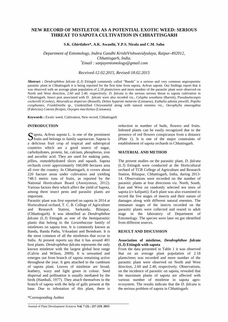
Abstract : Dendrophthoe falcata (L.f) Ettingsh commonly called “Banda” is a serious and very common angiospermic

parasitic plant in Chhattisgarh it is being reported for the first time from sapota, Achras sapota. Our findings report that it

was observed with an average plant population of 2.18 plants/trees and more number of the parasitic plant were observed on

North and West direction, 2.60 and 2.40, respectively. D. falcata is the serious serious threat to sapota cultivation in

Chhattisgarh. Insect pest associated with D. falcate were also recoded viz., Celypha woodiana (Barrett), Pseudaulacaspis

cockerelli (Cooley), Aleurodicus disperses (Russell), Delias hyparete metarete (Linnaeus), Euthalia adonia pinwilli, Papilio

cresphontes, Frankliniella sp., Unidentified Chrysomelid along with natural enemies viz., Oecophylla smaragdina

(Fabricius) Cotesia flevipes, Oxyopes macilentus (Linnaeus).

Keywords : Exotic weed, Cultivation, New record, Chhattisgarh

INTRODUCTION

apota, Achras sapota L. is one of the prominent

fruits and belongs to family sapotaceae. Sapota is

a delicious fruit crop of tropical and subtropical

countries which are a good source of sugar,

carbohydrates, protein, fat, calcium, phosphorus, iron

and ascorbic acid. They are used for making jams,

jellies, osmodehydrated slices and squash. Sapota

orchards cover approximately 160,000 hectares area

all over the country. In Chhattisgarh, it covers about

220 hactare areas under cultivation and yielding

748.5 metric tons of fruits, as reported by the

National Horticulture Board (Anonymous, 2012).

Various factors their which affect the yield of Sapota,

among them insect pests and parasitic plants are

important.

Parasitic plant was first reported on sapota in 2014 at

Horticultural orchard, T. C. B. College of Agriculture

and Research Station, Sarkanda, Bilaspur,

(Chhattisgarh). It was identified as Dendrophthoe

falcata (L.f) Ettingsh as one of the hemiparasitic

plants that belong to the Loranthaceae family of

mistletoes on sapota tree. It is commonly known as

Banda, Banda Patha, Vrksadani and Bemdram. It is

the most common of all the mistletoes that occur in

India. At present reports say that it has around 401

host plants. Dendrophthoe falcata represents the only

known mistletoe with the largest global host range

(Calvin and Wilson, 2009). It is unwanted and

emerges out from branch of sapota remaining active

throughout the year. It gets attached to the cambium

of sapota plant. Leaves of mistletoe are broad,

leathery, waxy and light green in colour. Seed

dispersal and pollination is usually mediated by the

birds (Hambali, 1977). They attach themselves to the

branch of sapota with the help of galls present at the

base. Due to infestation of this plant, there is

reduction in number of buds, flowers and fruits.

Infested plants can be easily recognized due to the

presence of red flowers conspicuous from a distance

(Plate 1). It is one of the major constraints of

establishment of sapota orchards in Chhattisgarh.

MATERIAL AND METHOD

The present studies on the parasitic plant, D. falcata

(L.f) Ettingsh were conducted at the Horticultural

orchard of TCB College of Agriculture and Research

Station, Bilaspur, Chhattisgarh, India, during 2013-

14. Observations were recorded on the number of

parasitic plants at four directions viz. North, South,

East and West on randomly selected ten trees of

sapota (cv kalipatti). Each plant was also examined to

record the live stages of insects and their nature of

damages along with different natural enemies. The

immature stages of the insects recorded on the

parasitic plants were collected and reared to adult

stage in the laboratory of Department of

Entomology. The species were later on got identified

from different sources.


Association of mistletoe, Dendrophthoe falcata

(L.f) Ettingsh with sapota

From the data presented in Table 1 it was observed

that on an average plant population of 2.18

plants/trees was recorded and more number of the

parasitic plant were observed on North and West

direction, 2.60 and 2.40, respectively. Observations,

on the incidence of parasitic on sapota, revealed that

the maximum plants of sapota are affected with

various number of mistletoe in sapota agro-

ecosystem. The results indicate that the D. falcata is

the serious problem of sapota in Chhattisgarh.

S

mailto:[email protected]

http://en.wikipedia.org/wiki/Hemiparasite

http://en.wikipedia.org/wiki/Loranthaceae

http://en.wikipedia.org/wiki/Mistletoe

http://en.wikipedia.org/wiki/India

http://en.wikipedia.org/wiki/Host_range

http://en.wikipedia.org/wiki/Pollination

218 S.K. GHIRTLAHRE, A.K. AWASTHI, Y.P.S. NIRALA AND C.M. SAHU

Record of insect pests and their natural enemies

on mistletoe, Dendrophthoe falcate

During the experiment eight insects were recorded on

parasitic plants viz. Marble moth, Celypha woodiana

(Barrett), False oleanderscale, Pseudaulacaspis

cockerelli (Cooley), Spiralling whitefly, Aleurodicus

disperses (Russell), Painted Jezebel butterfly, Delias

hyparete metarete (Linnaeus), Green Baron, Euthalia

adonia pinwilli, Giant swallowtail caterpillar, Papilio

cresphontes, Thrips, Frankliniella sp., Unidentified

Chrysomelid and few natural enemies were also

observed associated with above mentioned insect

pests viz., Red ant, Oecophylla smaragdina

(Fabricius), Apenteles, Cotesia flevipes and Lynx

Spider, Oxyopes macilentus (Linnaeus).

Table 1. Number of misteltoe/plants of Sapota, Achras sapota L.

S.No. North South East West Mean

1 3 0 3 1 1.75

2 4 2 0 0 1.50

3 2 1 3 2 2.0

4 1 0 4 1 1.50

5 3 0 1 5 2.25

6 0 4 5 1 2.50

7 5 2 1 4 3.0

8 2 1 0 2 1.25

9 0 5 0 6 2.75

10 6 3 2 2 3.25

Mean 2.60 1.80 1.90 2.40 2.18

Table 2. Record of insect pests of mistletoe, Dendrophthoe falcate

S.N. Insect pests Scientific Name Order Family

1 Marble moth Celypha woodiana Barrett Lepidoptera Tortricidae

2 False oleanderscale Pseudaulacaspis cockerelli Cooley Hemiptera Diaspididae

3 Spiralling whitefly Aleurodicus disperses Russell Hemiptera Aleyrodidae

4 Painted Jezebel butterfly Delias hyparete metarete Linnaeus Lepidoptera Pieridae

5 Green Baron Euthalia adonia pinwilli Lepidoptera Nymphalidae

6 Giant swallowtail

caterpillar

Papilio cresphontes Lepidoptera Papilionidae

7 Thrips Frankliniella sp. Thysenoptera Thripidae

8 Chrysomelid beetle Unidentified Coleoptera Chrysomelidae

Natural enemies :

1 Red ant Oecophylla smaragdina Fabricius Hymenoptera Formicidae

2 Apenteles Cotesia flevipes Hymenoptera Braconidea

3 Lynx Spider Oxyopes macilentus L. Araneae Araneidae


REFERENCES

Anonymous (2012). Directorate of Horticulture.

Raipur, Chhattisgarh.

Calvin,C.L., Wilson, C.A. (2009). Epiparasitism in

Phoradendron durangense and P. falcatum

(Viscaceae) Aliso, 27:1–12.

Hambali, G. G. (1977). On mistletoe parasitism.

Proceedings of the 6th Asian-Pacific Weed Science

Society Conference, Indonesia, 58–66.

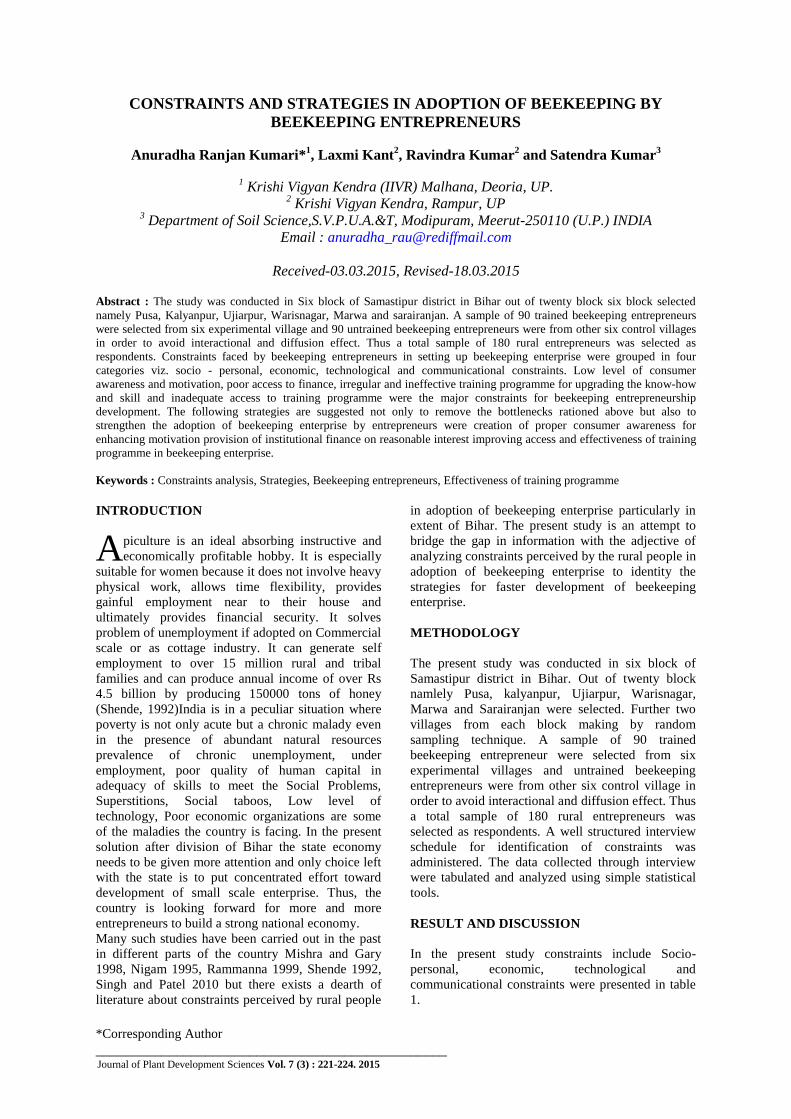
Plate 6. Cotesia flevipes a larval parasitoid of Celypha

woodiana

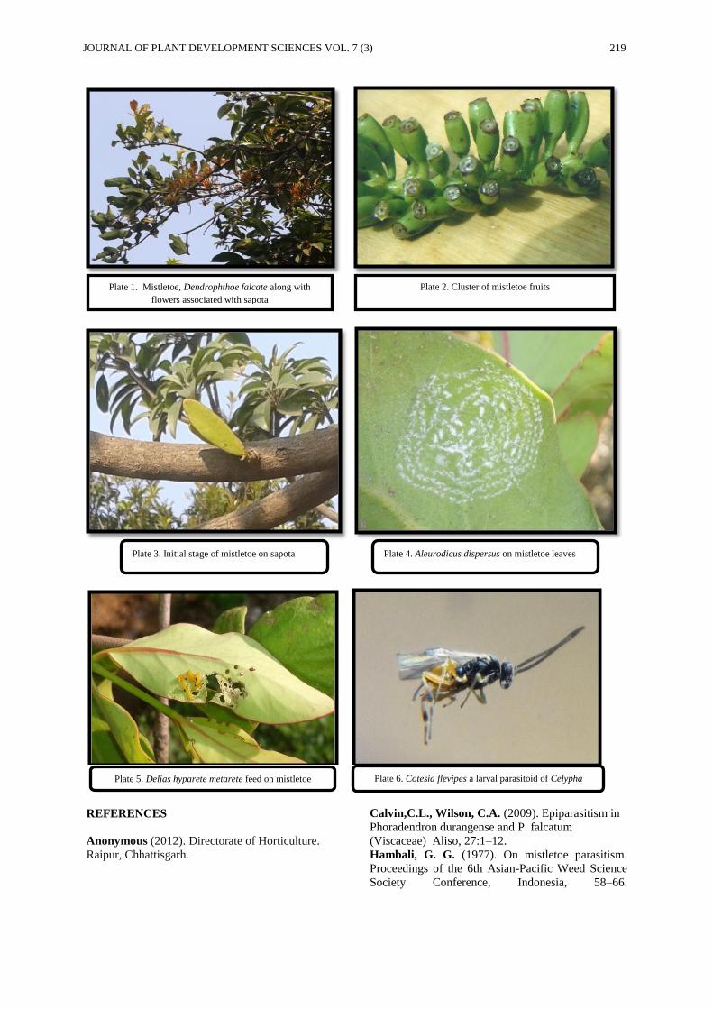
Plate 5. Delias hyparete metarete feed on mistletoe

leaves

Plate 4. Aleurodicus dispersus on mistletoe leaves Plate 3. Initial stage of mistletoe on sapota

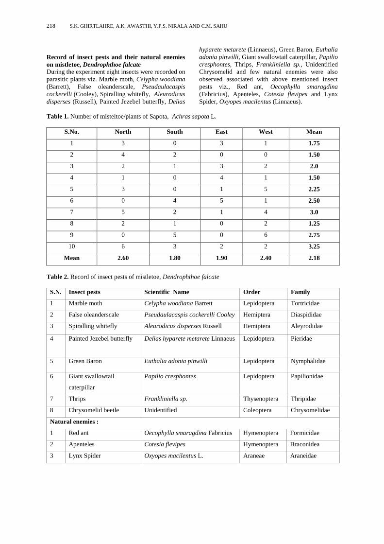
Plate 2. Cluster of mistletoe fruits Plate 1. Mistletoe, Dendrophthoe falcate along with

flowers associated with sapota

220 S.K. GHIRTLAHRE, A.K. AWASTHI, Y.P.S. NIRALA AND C.M. SAHU



CONSTRAINTS AND STRATEGIES IN ADOPTION OF BEEKEEPING BY

BEEKEEPING ENTREPRENEURS

Anuradha Ranjan Kumari*1, Laxmi Kant

2, Ravindra Kumar

2 and Satendra Kumar

3

1 Krishi Vigyan Kendra (IIVR) Malhana, Deoria, UP.

2 Krishi Vigyan Kendra, Rampur, UP

3 Department of Soil Science,S.V.P.U.A.&T, Modipuram, Meerut-250110 (U.P.) INDIA

Email : [email protected]


Abstract : The study was conducted in Six block of Samastipur district in Bihar out of twenty block six block selected

namely Pusa, Kalyanpur, Ujiarpur, Warisnagar, Marwa and sarairanjan. A sample of 90 trained beekeeping entrepreneurs

were selected from six experimental village and 90 untrained beekeeping entrepreneurs were from other six control villages

in order to avoid interactional and diffusion effect. Thus a total sample of 180 rural entrepreneurs was selected as

respondents. Constraints faced by beekeeping entrepreneurs in setting up beekeeping enterprise were grouped in four

categories viz. socio - personal, economic, technological and communicational constraints. Low level of consumer

awareness and motivation, poor access to finance, irregular and ineffective training programme for upgrading the know-how

and skill and inadequate access to training programme were the major constraints for beekeeping entrepreneurship

development. The following strategies are suggested not only to remove the bottlenecks rationed above but also to

strengthen the adoption of beekeeping enterprise by entrepreneurs were creation of proper consumer awareness for

enhancing motivation provision of institutional finance on reasonable interest improving access and effectiveness of training

programme in beekeeping enterprise.

Keywords : Constraints analysis, Strategies, Beekeeping entrepreneurs, Effectiveness of training programme

INTRODUCTION

piculture is an ideal absorbing instructive and

economically profitable hobby. It is especially

suitable for women because it does not involve heavy

physical work, allows time flexibility, provides

gainful employment near to their house and

ultimately provides financial security. It solves

problem of unemployment if adopted on Commercial

scale or as cottage industry. It can generate self

employment to over 15 million rural and tribal

families and can produce annual income of over Rs

4.5 billion by producing 150000 tons of honey

(Shende, 1992)India is in a peculiar situation where

poverty is not only acute but a chronic malady even

in the presence of abundant natural resources

prevalence of chronic unemployment, under

employment, poor quality of human capital in

adequacy of skills to meet the Social Problems,

Superstitions, Social taboos, Low level of

technology, Poor economic organizations are some

of the maladies the country is facing. In the present

solution after division of Bihar the state economy

needs to be given more attention and only choice left

with the state is to put concentrated effort toward

development of small scale enterprise. Thus, the

country is looking forward for more and more

entrepreneurs to build a strong national economy.

Many such studies have been carried out in the past

in different parts of the country Mishra and Gary

1998, Nigam 1995, Rammanna 1999, Shende 1992,

Singh and Patel 2010 but there exists a dearth of

literature about constraints perceived by rural people

in adoption of beekeeping enterprise particularly in

extent of Bihar. The present study is an attempt to

bridge the gap in information with the adjective of

analyzing constraints perceived by the rural people in

adoption of beekeeping enterprise to identity the

strategies for faster development of beekeeping

enterprise.

METHODOLOGY

The present study was conducted in six block of

Samastipur district in Bihar. Out of twenty block

namlely Pusa, kalyanpur, Ujiarpur, Warisnagar,

Marwa and Sarairanjan were selected. Further two

villages from each block making by random

sampling technique. A sample of 90 trained

beekeeping entrepreneur were selected from six

experimental villages and untrained beekeeping

entrepreneurs were from other six control village in

order to avoid interactional and diffusion effect. Thus

a total sample of 180 rural entrepreneurs was

selected as respondents. A well structured interview

schedule for identification of constraints was

administered. The data collected through interview

were tabulated and analyzed using simple statistical

tools.


In the present study constraints include Socio-

personal, economic, technological and

communicational constraints were presented in table

1.

A


222 ANURADHA RANJAN KUMARI, LAXMI KANT, RAVINDRA KUMAR AND SATENDRA KUMAR

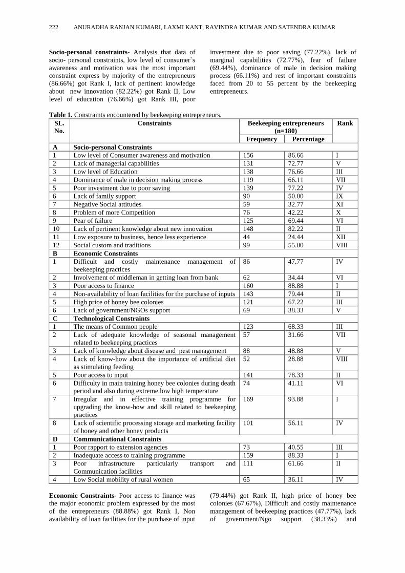
Socio-personal constraints- Analysis that data of

socio- personal constraints, low level of consumer`s

awareness and motivation was the most important

constraint express by majority of the entrepreneurs

(86.66%) got Rank I, lack of pertinent knowledge

about new innovation (82.22%) got Rank II, Low

level of education (76.66%) got Rank III, poor

investment due to poor saving (77.22%), lack of

marginal capabilities (72.77%), fear of failure

(69.44%), dominance of male in decision making

process (66.11%) and rest of important constraints

faced from 20 to 55 percent by the beekeeping

entrepreneurs.

Table 1. Constraints encountered by beekeeping entrepreneurs.

SL.

No.

Constraints Beekeeping entrepreneurs

(n=180)

Rank

Frequency Percentage

A Socio-personal Constraints

1 Low level of Consumer awareness and motivation 156 86.66 I

2 Lack of managerial capabilities 131 72.77 V

3 Low level of Education 138 76.66 III

4 Dominance of male in decision making process 119 66.11 VII

5 Poor investment due to poor saving 139 77.22 IV

6 Lack of family support 90 50.00 IX

7 Negative Social attitudes 59 32.77 XI

8 Problem of more Competition 76 42.22 X

9 Pear of failure 125 69.44 VI

10 Lack of pertinent knowledge about new innovation 148 82.22 II

11 Low exposure to business, hence less experience 44 24.44 XII

12 Social custom and traditions 99 55.00 VIII

B Economic Constraints

1 Difficult and costly maintenance management of

beekeeping practices

86 47.77 IV

2 Involvement of middleman in getting loan from bank 62 34.44 VI

3 Poor access to finance 160 88.88 I

4 Non-availability of loan facilities for the purchase of inputs 143 79.44 II

5 High price of honey bee colonies 121 67.22 III

6 Lack of government/NGOs support 69 38.33 V

C Technological Constraints

1 The means of Common people 123 68.33 III

2 Lack of adequate knowledge of seasonal management

related to beekeeping practices

57 31.66 VII

3 Lack of knowledge about disease and pest management 88 48.88 V

4 Lack of know-how about the importance of artificial diet

as stimulating feeding

52 28.88 VIII

5 Poor access to input 141 78.33 II

6 Difficulty in main training honey bee colonies during death

period and also during extreme low high temperature

74 41.11 VI

7 Irregular and in effective training programme for

upgrading the know-how and skill related to beekeeping

practices

169 93.88 I

8 Lack of scientific processing storage and marketing facility

of honey and other honey products

101 56.11 IV

D Communicational Constraints

1 Poor rapport to extension agencies 73 40.55 III

2 Inadequate access to training programme 159 88.33 I

3 Poor infrastructure particularly transport and

Communication facilities

111 61.66 II

4 Low Social mobility of rural women 65 36.11 IV

Economic Constraints- Poor access to finance was

the major economic problem expressed by the most

of the entrepreneurs (88.88%) got Rank I, Non

availability of loan facilities for the purchase of input

(79.44%) got Rank II, high price of honey bee

colonies (67.67%), Difficult and costly maintenance

management of beekeeping practices (47.77%), lack

of government/Ngo support (38.33%) and


involvement of middleman in getting loan from bank

(34.44%) got last rank were also constraints in

establishing beekeeping enterprises.

Technological Constraints- From perusal of table 1

it evident that the technological constraints were left

by most of the entrepreneurs irregular and ineffective

training programme for upgrading the knowhow and

skill related to beekeeping enterprise was observed as

major technical constraints since it was expressed by

majority of the entrepreneurs (93.88%) followed by

poor access to input (78.33%) and technology

(68.33%) got rank III and rest got the rank IV to VIII

in different technological Constraints.

Communicational Constraints- Under the

Communicational constraints inadequate access to

training programme (88.33%) got the rank I was

found as major constraints. Poor infrastructure

particularly transport and communication facilities

(61.66%) poor rapport to extension agencies

(44.55%) and low social mobility of rural women

(36.11%) got last rank IV were also the important

constraint (Table 1)

Strategies

Constraints which prevent beekeeping entrepreneurs

in starting self employment necessitate the need to

design development strategies. The following

strategies are suggested not only to remove the

bottlenecks mentioned above but also to strengthen

the adoption of beekeeping enterprise by

entrepreneurs strategies suggested by respondents for

development of entrepreneurship among rural people

should address all these aspects.

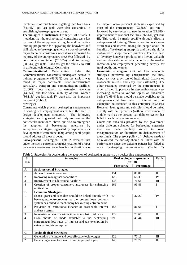
Socio-personal strategies- Table 2 revealed that

under the socio personal strategies creation of proper

consumers awareness for enhancing motivation was

the major Socio- personal strategies expressed by

most of the entrepreneurs (93.88%) got rank I

followed by easy access to new innovation (83.88%)

improvement educational facilities (76.66%) got rank

III. This could be made possible through effective

entrepreneurial training. There is need to create more

awareness and interest among the people about the

benefits of beekeeping enterprise and they should be

motivated to adopt modern practices. There is need

to diversify honeybee products to different valuable

and nutritive substances which could also be used as

recreation and employment generating activity for

rural youths and women.

Economic strategies- Out of four economic

strategies perceived by entrepreneurs the most

important was provision of institutional finance on

reasonable interest and easy terms (88.66%). The

other strategies perceived by the entrepreneurs in

order of their importance in descending order were

increasing access to various inputs on subsidized

basis (71.66%) loan should be made available to the

entrepreneurs at low rates of interest and tax

exemption be extended to this enterprise (49.44%).

However, loan, grants and subsidies should be linked

directly with entrepreneurs (without involvement of

middle man) as the present loan delivery system has

failed to each many entrepreneurs.

Grants and subsidies provided by the government

under different schemes for beekeeping enterprise

also are made publicly known to avoid

misappropriation or favoritism in disbursement of

these funds. The present policy of subsidies needs to

be reviewed; the subsidy should be linked with the

performance since the existing pattern has failed to

raise beekeeping entrepreneurs (Table 2).

Table 2. Strategies for accelerating the adoption of beekeeping enterprise by beekeeping entrepreneurs.

Sl.

No.

Strategies Beekeeping entrepreneurs

(n=180)

Rank

Frequency Percentage

A Socio-personal Strategies

1 Access to new innovation 151 83.88 II

2 Improving managerial capabilities 123 68.33 IV

3 Improvement in educational facilities 138 76.66 III

4 Creation of proper consumers awareness for enhancing

motivation

169 93.88 I

B Economic Strategies

1 Loans, grant and subsidies should be linked directly with

beekeeping entrepreneurs as the present loan delivery

system has failed to reach many beekeeping entrepreneurs

67 37.22 IV

2 Provision of institutional Finance on reasonable interest

and easy terms.

156 86.66 I

3 Increasing access to various inputs on subsidized basis 129 73.66 II

4 Loan should be made available to the beekeeping

entrepreneur low rates of interest and tax exemption be

extended to this enterprise

89 49.44 III

C Technological Strategies

1 Generation of simple and cost effective technologies 128 71.11 III

2 Enhancing access to scientific and improved inputs 140 77.77 II

224 ANURADHA RANJAN KUMARI, LAXMI KANT, RAVINDRA KUMAR AND SATENDRA KUMAR

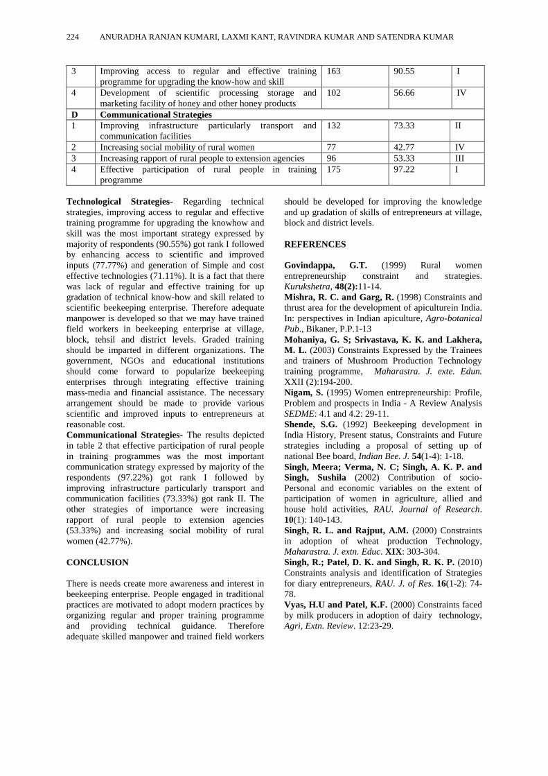
3 Improving access to regular and effective training

programme for upgrading the know-how and skill

163 90.55 I

4 Development of scientific processing storage and

marketing facility of honey and other honey products

102 56.66 IV

D Communicational Strategies

1 Improving infrastructure particularly transport and

communication facilities

132 73.33 II

2 Increasing social mobility of rural women 77 42.77 IV

3 Increasing rapport of rural people to extension agencies 96 53.33 III

4 Effective participation of rural people in training

programme

175 97.22 I

Technological Strategies- Regarding technical

strategies, improving access to regular and effective

training programme for upgrading the knowhow and

skill was the most important strategy expressed by

majority of respondents (90.55%) got rank I followed

by enhancing access to scientific and improved

inputs (77.77%) and generation of Simple and cost

effective technologies (71.11%). It is a fact that there

was lack of regular and effective training for up

gradation of technical know-how and skill related to

scientific beekeeping enterprise. Therefore adequate

manpower is developed so that we may have trained

field workers in beekeeping enterprise at village,

block, tehsil and district levels. Graded training

should be imparted in different organizations. The

government, NGOs and educational institutions

should come forward to popularize beekeeping

enterprises through integrating effective training

mass-media and financial assistance. The necessary

arrangement should be made to provide various

scientific and improved inputs to entrepreneurs at

reasonable cost.

Communicational Strategies- The results depicted

in table 2 that effective participation of rural people

in training programmes was the most important

communication strategy expressed by majority of the

respondents (97.22%) got rank I followed by

improving infrastructure particularly transport and

communication facilities (73.33%) got rank II. The

other strategies of importance were increasing

rapport of rural people to extension agencies

(53.33%) and increasing social mobility of rural

women (42.77%).

CONCLUSION

There is needs create more awareness and interest in

beekeeping enterprise. People engaged in traditional

practices are motivated to adopt modern practices by

organizing regular and proper training programme

and providing technical guidance. Therefore

adequate skilled manpower and trained field workers

should be developed for improving the knowledge

and up gradation of skills of entrepreneurs at village,

block and district levels.

REFERENCES

Govindappa, G.T. (1999) Rural women

entrepreneurship constraint and strategies.

Kurukshetra, 48(2):11-14.

Mishra, R. C. and Garg, R. (1998) Constraints and

thrust area for the development of apiculturein India.

In: perspectives in Indian apiculture, Agro-botanical

Pub., Bikaner, P.P.1-13

Mohaniya, G. S; Srivastava, K. K. and Lakhera,

M. L. (2003) Constraints Expressed by the Trainees

and trainers of Mushroom Production Technology

training programme, Maharastra. J. exte. Edun.

XXII (2):194-200.

Nigam, S. (1995) Women entrepreneurship: Profile,

Problem and prospects in India - A Review Analysis

SEDME: 4.1 and 4.2: 29-11.

Shende, S.G. (1992) Beekeeping development in

India History, Present status, Constraints and Future

strategies including a proposal of setting up of

national Bee board, Indian Bee. J. 54(1-4): 1-18.

Singh, Meera; Verma, N. C; Singh, A. K. P. and

Singh, Sushila (2002) Contribution of socio-

Personal and economic variables on the extent of

participation of women in agriculture, allied and

house hold activities, RAU. Journal of Research.

10(1): 140-143.

Singh, R. L. and Rajput, A.M. (2000) Constraints

in adoption of wheat production Technology,

Maharastra. J. extn. Educ. XIX: 303-304.

Singh, R.; Patel, D. K. and Singh, R. K. P. (2010)

Constraints analysis and identification of Strategies

for diary entrepreneurs, RAU. J. of Res. 16(1-2): 74-

78.

Vyas, H.U and Patel, K.F. (2000) Constraints faced

by milk producers in adoption of dairy technology,

Agri, Extn. Review. 12:23-29.



STUDY ON COMPARATIVE PERFORMANCE OF FINE SLENDER RICE

GENOTYPES AGAINST RICE GALL MIDGE IN THE NORTHERN HILL REGION

OF C.G.

Jai Kishan Bhagat* and Rahul Harinkhere

Department of Entomology, College of Agriculture, IGKV, Raipur-492012 (CG)


Abstracts : A part from food, rice is intimately involved in the culture as well as economy of many societies. The cultivation

of rice is done under more diverse conditions than any other food crop, ranging from irrigated to rainfed ecology and upland

to deep water conditions. In world, rice has occupied an area of 154 million hectares, with a total production of 476 million

tonnes and productivity 2949 kg ha-1 (Anonymous, 2012). India has largest area among rice growing countries and enjoys

the second rank in production. India has 45.5 million hectares, total cultivated area under rice, with the production of 105.31

million tonnes and productivity 2393 kg ha-1 (Anonymous, 2013 a). Chhattisgarh state is popularly known as “rice bowl of

India” because maximum area is covered under rice during Kharif and contribute major share in national rice production. It

has geographical area of 13.51 million hectares of which 5.9 million hectares area is under cultivation. Rice occupies an area

around 3.61 million hectares, with the production of 5.48 million tonnes and productivity 1517 kg ha-1 (Anonymous, 2013b).

Keywords : Hill region, Genotypes, Rice

INTRODUCTION

he productivity of rice in Chhattisgarh is

comparatively lower than the national average.

This is due to several constraints which are

responsible for such low productivity rice in the

region. Among these, insect pests are one of the most

important factors limiting the rice production. There

are more than 100 species of insect pests of rice but

only about 20 of them are of major economic

importance (Pathak and Khush, 1979). The losses

due to insect pests during vegetative phase (50

percentage) contributes more to yield reduction than

the reproductive phase (30 percentage) or ripening

phase (20 percentage) as reported by Gupta and

Raghuraman (2003). In Chhattisgarh region various

rice pests cause losses up to 20 percentages every

year to rice crop. Which gall midge, Orseolia oryzae

(Wood-Mason), The Asian rice gall midge, Orseolia

oryzae (Wood-Mason), Diptera: Cecidomyidae, is

the most important pest and causes extensive

damage. (Jagadeesha Kumar et. al., 2009). It is an

important pest from the seed bed to maximum

tillering stages of the rice crop. Yield loss

assessments in field with up to 30% tiller infestation

suggest that for each 1% increase in tiller infestation,

a farmer can expect to lose 2-3% grain yield, (Nacro

et al., 1996). In Chhattisgarh rice gall midge is

locally called “gangai”. The extent of losses it cause

has been recorded from as low as a few kilograms to

as high as 25 q/ha (Kittur and Agrawal, 1983). The

major active period of these insect is September to

October. In rice gall midge, maggot is the destructive

stage and the feeding maggot causes the conversion

of leaf sheath to galls often referred as „onion shoots'

or „silvershoots‟ (Hidaka, 1974 and Hill, 1987) and it

also causes the production of secondary tillers which

may themselves become infested. In India, gall

midge is a serious pest of irrigated and shallow water

rice ecosystem (Lai et al., 1984). In Chhattisgarh

region gall midge caused 30 to 40 per cent losses in

yield in susceptible varieties of paddy (Anonymous,

2010).

Therefore, ‘‘study on comparative performance of

fine slender rice genotypes against rice gall midge in

the northern region of C, G.” is undertaken for the

present investigation

MATERIAL AND METHOD

Site and Climate

Ambikapur is an important rice growing tract of

Chhattisgarh and comes under the northern hill

region of Chhattishgarh in India. The general climate

condition of Surguja is Eastern plateau and hilly

region with average rainfall 1422.8 mm.

Experimental details Place of experiment : Ajirma Research Farm RMD CARS, Ambikapur.

Crop : Rice

Date of sowing : 11-07-2013

Date of transplanting : 01-08-2013

Season : Kharif, 2013

Design : Randomized Block Design

Replications : 03

T

226 JAI KISHAN BHAGAT AND RAHUL HARINKHERE

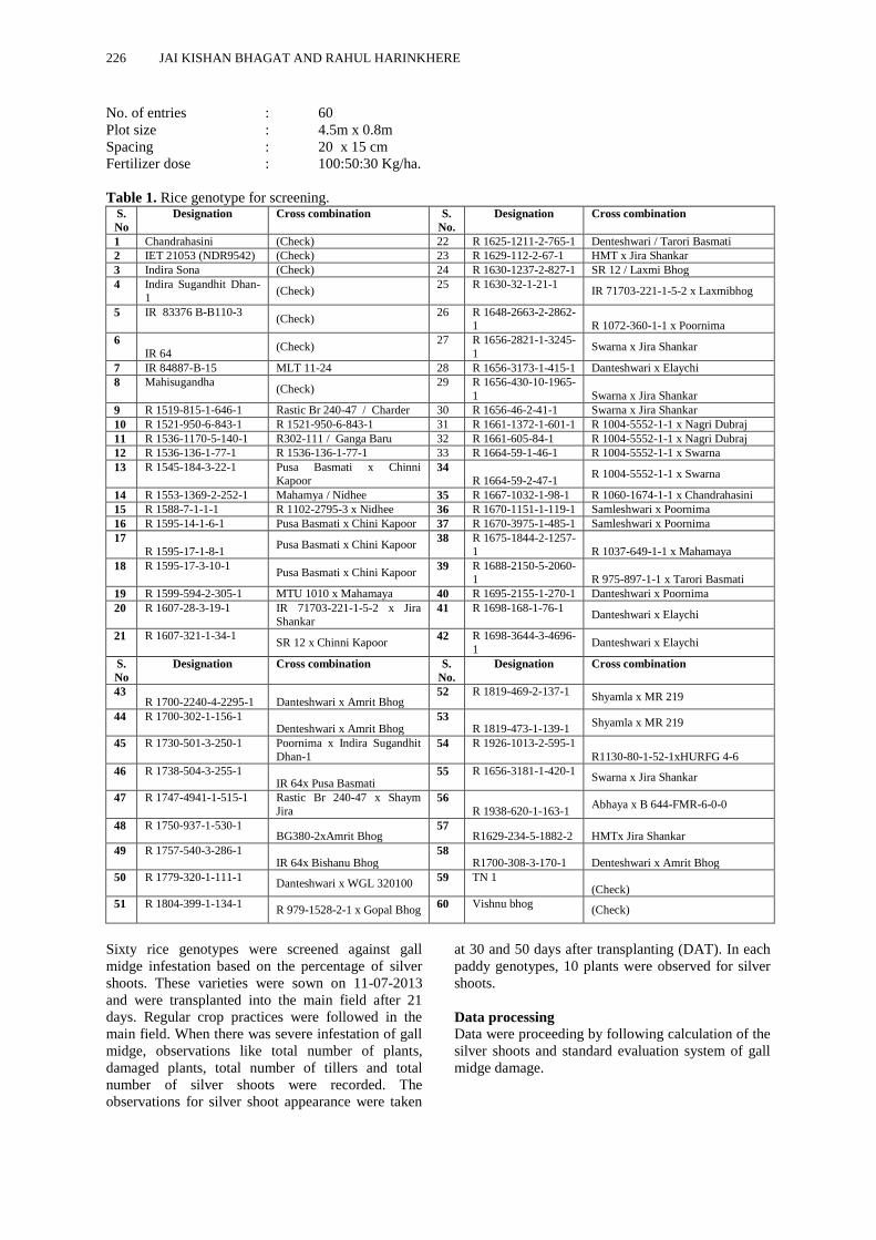
No. of entries : 60

Plot size : 4.5m x 0.8m

Spacing : 20 x 15 cm

Fertilizer dose : 100:50:30 Kg/ha.

Table 1. Rice genotype for screening. S.

No

Designation Cross combination S.

No.

Designation Cross combination

1 Chandrahasini (Check) 22 R 1625-1211-2-765-1 Denteshwari / Tarori Basmati

2 IET 21053 (NDR9542) (Check) 23 R 1629-112-2-67-1 HMT x Jira Shankar

3 Indira Sona (Check) 24 R 1630-1237-2-827-1 SR 12 / Laxmi Bhog

4 Indira Sugandhit Dhan-

1 (Check)

25 R 1630-32-1-21-1 IR 71703-221-1-5-2 x Laxmibhog

5 IR 83376 B-B110-3 (Check)

26 R 1648-2663-2-2862-1 R 1072-360-1-1 x Poornima

6

IR 64 (Check)

27 R 1656-2821-1-3245-

1 Swarna x Jira Shankar

7 IR 84887-B-15 MLT 11-24 28 R 1656-3173-1-415-1 Danteshwari x Elaychi

8 Mahisugandha (Check)

29 R 1656-430-10-1965-

1 Swarna x Jira Shankar

9 R 1519-815-1-646-1 Rastic Br 240-47 / Charder 30 R 1656-46-2-41-1 Swarna x Jira Shankar

10 R 1521-950-6-843-1 R 1521-950-6-843-1 31 R 1661-1372-1-601-1 R 1004-5552-1-1 x Nagri Dubraj

11 R 1536-1170-5-140-1 R302-111 / Ganga Baru 32 R 1661-605-84-1 R 1004-5552-1-1 x Nagri Dubraj

12 R 1536-136-1-77-1 R 1536-136-1-77-1 33 R 1664-59-1-46-1 R 1004-5552-1-1 x Swarna

13 R 1545-184-3-22-1 Pusa Basmati x Chinni

Kapoor 34

R 1664-59-2-47-1 R 1004-5552-1-1 x Swarna

14 R 1553-1369-2-252-1 Mahamya / Nidhee 35 R 1667-1032-1-98-1 R 1060-1674-1-1 x Chandrahasini

15 R 1588-7-1-1-1 R 1102-2795-3 x Nidhee 36 R 1670-1151-1-119-1 Samleshwari x Poornima

16 R 1595-14-1-6-1 Pusa Basmati x Chini Kapoor 37 R 1670-3975-1-485-1 Samleshwari x Poornima

17

R 1595-17-1-8-1 Pusa Basmati x Chini Kapoor

38 R 1675-1844-2-1257-

1 R 1037-649-1-1 x Mahamaya

18 R 1595-17-3-10-1 Pusa Basmati x Chini Kapoor

39 R 1688-2150-5-2060-1 R 975-897-1-1 x Tarori Basmati

19 R 1599-594-2-305-1 MTU 1010 x Mahamaya 40 R 1695-2155-1-270-1 Danteshwari x Poornima

20 R 1607-28-3-19-1 IR 71703-221-1-5-2 x Jira

Shankar 41 R 1698-168-1-76-1

Danteshwari x Elaychi

21 R 1607-321-1-34-1 SR 12 x Chinni Kapoor

42 R 1698-3644-3-4696-

1 Danteshwari x Elaychi

S.

No

Designation Cross combination S.

No.

Designation Cross combination

43 R 1700-2240-4-2295-1 Danteshwari x Amrit Bhog

52 R 1819-469-2-137-1 Shyamla x MR 219

44 R 1700-302-1-156-1 Denteshwari x Amrit Bhog

53 R 1819-473-1-139-1

Shyamla x MR 219

45 R 1730-501-3-250-1 Poornima x Indira Sugandhit

Dhan-1 54 R 1926-1013-2-595-1

R1130-80-1-52-1xHURFG 4-6

46 R 1738-504-3-255-1 IR 64x Pusa Basmati

55 R 1656-3181-1-420-1 Swarna x Jira Shankar

47 R 1747-4941-1-515-1 Rastic Br 240-47 x Shaym

Jira 56

R 1938-620-1-163-1 Abhaya x B 644-FMR-6-0-0

48 R 1750-937-1-530-1 BG380-2xAmrit Bhog

57 R1629-234-5-1882-2 HMTx Jira Shankar

49 R 1757-540-3-286-1 IR 64x Bishanu Bhog

58 R1700-308-3-170-1 Denteshwari x Amrit Bhog

50 R 1779-320-1-111-1 Danteshwari x WGL 320100

59 TN 1 (Check)

51 R 1804-399-1-134-1 R 979-1528-2-1 x Gopal Bhog

60 Vishnu bhog (Check)

Sixty rice genotypes were screened against gall

midge infestation based on the percentage of silver

shoots. These varieties were sown on 11-07-2013

and were transplanted into the main field after 21

days. Regular crop practices were followed in the

main field. When there was severe infestation of gall

midge, observations like total number of plants,

damaged plants, total number of tillers and total

number of silver shoots were recorded. The

observations for silver shoot appearance were taken

at 30 and 50 days after transplanting (DAT). In each

paddy genotypes, 10 plants were observed for silver

shoots.

Data processing

Data were proceeding by following calculation of the

silver shoots and standard evaluation system of gall

midge damage.


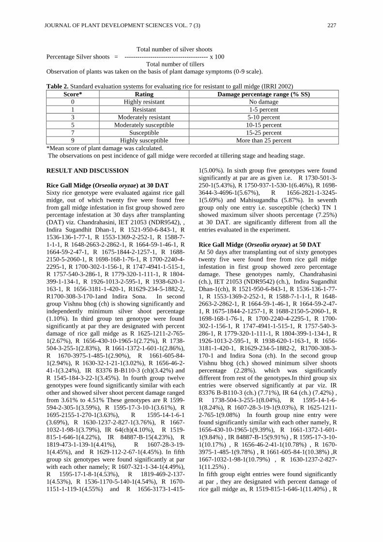
Total number of silver shoots

Percentage Silver shoots = --------------------------------------- x 100

Total number of tillers

Observation of plants was taken on the basis of plant damage symptoms (0-9 scale).

Table 2. Standard evaluation systems for evaluating rice for resistant to gall midge (IRRI 2002)

Score* Rating Damage percentage range (% SS)

0 Highly resistant No damage

1 Resistant 1-5 percent

3 Moderately resistant 5-10 percent

5 Moderately susceptible 10-15 percent

7 Susceptible 15-25 percent

9 Highly susceptible More than 25 percent

*Mean score of plant damage was calculated.

The observations on pest incidence of gall midge were recorded at tillering stage and heading stage.


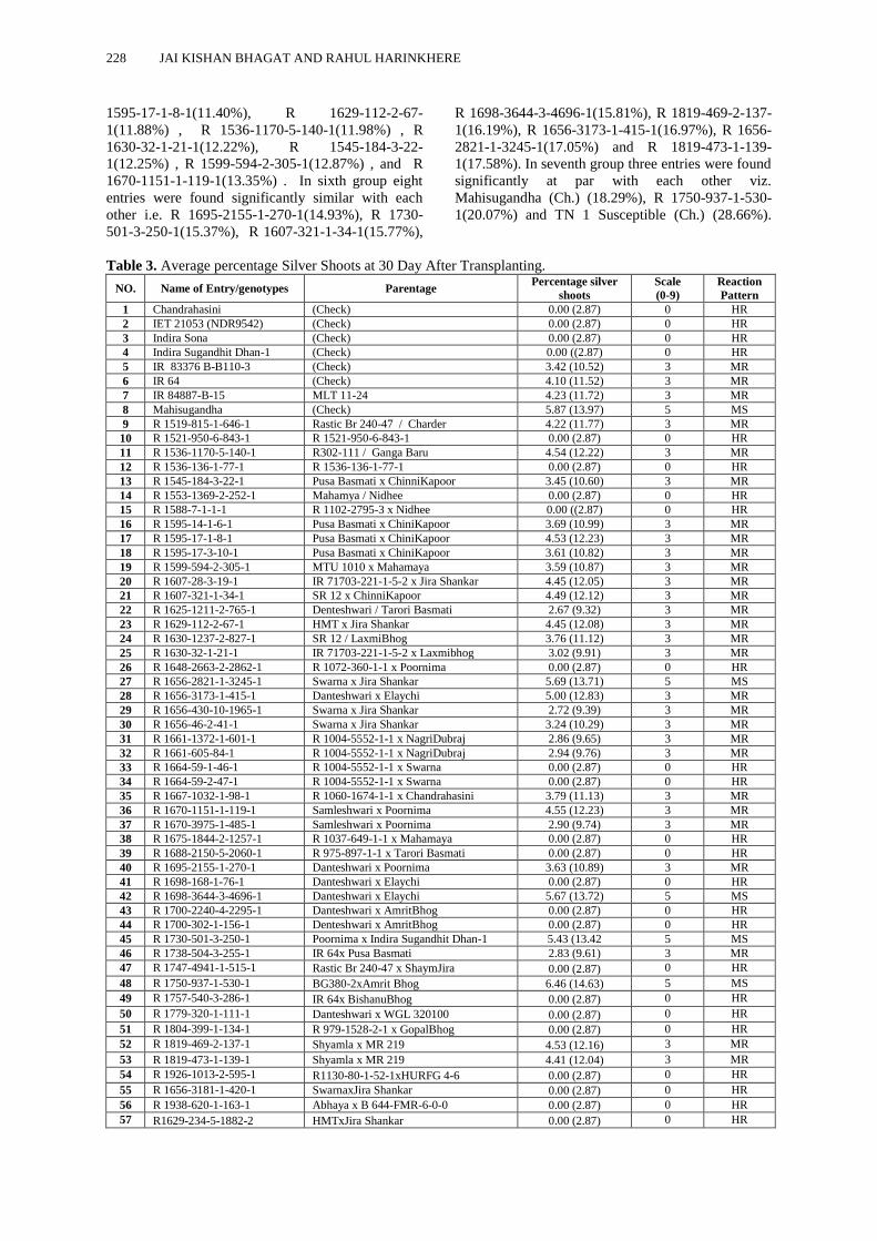
Rice Gall Midge (Orseolia oryzae) at 30 DAT

Sixty rice genotype were evaluated against rice gall

midge, out of which twenty five were found free

from gall midge infestation in fist group showed zero

percentage infestation at 30 days after transplanting

(DAT) viz. Chandrahasini, IET 21053 (NDR9542), ,

Indira Sugandhit Dhan-1, R 1521-950-6-843-1, R

1536-136-1-77-1, R 1553-1369-2-252-1, R 1588-7-

1-1-1, R 1648-2663-2-2862-1, R 1664-59-1-46-1, R

1664-59-2-47-1, R 1675-1844-2-1257-1, R 1688-

2150-5-2060-1, R 1698-168-1-76-1, R 1700-2240-4-

2295-1, R 1700-302-1-156-1, R 1747-4941-1-515-1,

R 1757-540-3-286-1, R 1779-320-1-111-1, R 1804-

399-1-134-1, R 1926-1013-2-595-1, R 1938-620-1-

163-1, R 1656-3181-1-420-1, R1629-234-5-1882-2,

R1700-308-3-170-1and Indira Sona. In second

group Vishnu bhog (ch) is showing significantly and

independently minimum silver shoot percentage

(1.10%). In third group ten genotype were found

significantly at par they are designated with percent

damage of rice gall midge as R 1625-1211-2-765-

1(2.67%), R 1656-430-10-1965-1(2.72%), R 1738-

504-3-255-1(2.83%), R 1661-1372-1-601-1(2.86%),

R 1670-3975-1-485-1(2.90%), R 1661-605-84-

1(2.94%), R 1630-32-1-21-1(3.02%), R 1656-46-2-

41-1(3.24%), IR 83376 B-B110-3 (ch)(3.42%) and

R 1545-184-3-22-1(3.45%). In fourth group twelve

genotypes were found significantly similar with each

other and showed silver shoot percent damage ranged

from 3.61% to 4.51% These genotypes are R 1599-

594-2-305-1(3.59%), R 1595-17-3-10-1(3.61%), R

1695-2155-1-270-1(3.63%), R 1595-14-1-6-1

(3.69%), R 1630-1237-2-827-1(3.76%), R 1667-

1032-1-98-1(3.79%), IR 64(ch)(4.10%), R 1519-

815-1-646-1(4.22%), IR 84887-B-15(4.23%), R

1819-473-1-139-1(4.41%), R 1607-28-3-19-

1(4.45%), and R 1629-112-2-67-1(4.45%). In fifth

group six genotypes were found significantly at par

with each other namely; R 1607-321-1-34-1(4.49%),

R 1595-17-1-8-1(4.53%), R 1819-469-2-137-

1(4.53%), R 1536-1170-5-140-1(4.54%), R 1670-

1151-1-119-1(4.55%) and R 1656-3173-1-415-

1(5.00%). In sixth group five genotypes were found

significantly at par are as given i.e. R 1730-501-3-

250-1(5.43%), R 1750-937-1-530-1(6.46%), R 1698-

3644-3-4696-1(5.67%), R 1656-2821-1-3245-

1(5.69%) and Mahisugandha (5.87%). In seventh

group only one entry i.e. susceptible (check) TN 1

showed maximum silver shoots percentage (7.25%)

at 30 DAT. are significantly different from all the

entries evaluated in the experiment.

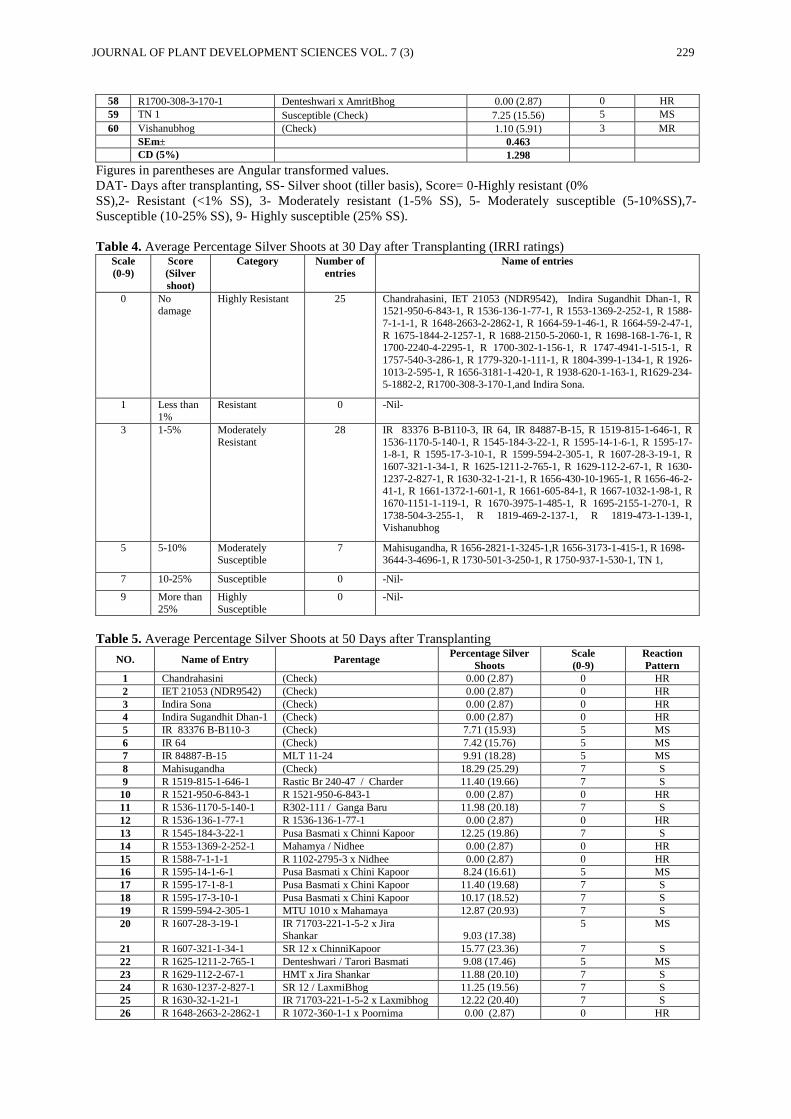
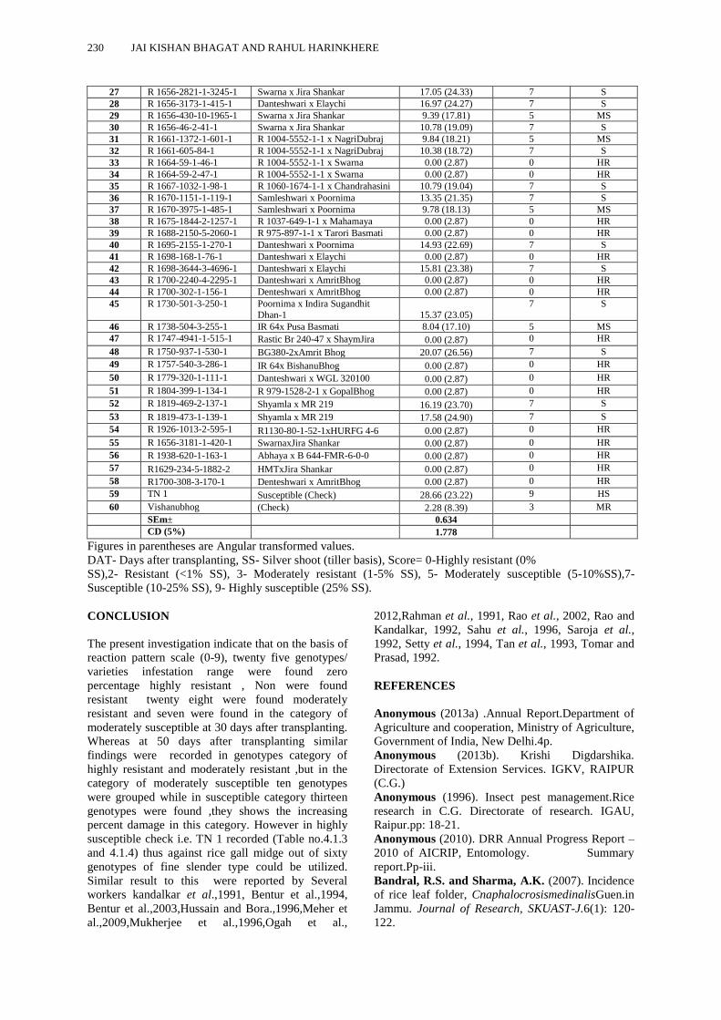
Rice Gall Midge (Orseolia oryzae) at 50 DAT

At 50 days after transplanting out of sixty genotypes

twenty five were found free from rice gall midge

infestation in first group showed zero percentage

damage. These genotypes namly, Chandrahasini

(ch.), IET 21053 (NDR9542) (ch.), Indira Sugandhit

Dhan-1(ch), R 1521-950-6-843-1, R 1536-136-1-77-

1, R 1553-1369-2-252-1, R 1588-7-1-1-1, R 1648-

2663-2-2862-1, R 1664-59-1-46-1, R 1664-59-2-47-

1, R 1675-1844-2-1257-1, R 1688-2150-5-2060-1, R

1698-168-1-76-1, R 1700-2240-4-2295-1, R 1700-

302-1-156-1, R 1747-4941-1-515-1, R 1757-540-3-

286-1, R 1779-320-1-111-1, R 1804-399-1-134-1, R

1926-1013-2-595-1, R 1938-620-1-163-1, R 1656-

3181-1-420-1, R1629-234-5-1882-2, R1700-308-3-

170-1 and Indira Sona (ch). In the second group

Vishnu bhog (ch.) showed minimum silver shoots

percentage (2.28%). which was significantly

different from rest of the genotypes.In third group six

entries were observed significantly at par viz. IR

83376 B-B110-3 (ch.) (7.71%), IR 64 (ch.) (7.42%) ,

R 1738-504-3-255-1(8.04%), R 1595-14-1-6-

1(8.24%), R 1607-28-3-19-1(9.03%), R 1625-1211-

2-765-1(9.08%) In fourth group nine entry were

found significantly similar with each other namely, R

1656-430-10-1965-1(9.39%), R 1661-1372-1-601-

1(9.84%) , IR 84887-B-15(9.91%) , R 1595-17-3-10-

1(10.17%) , R 1656-46-2-41-1(10.78%) , R 1670-

3975-1-485-1(9.78%) , R 1661-605-84-1(10.38%) ,R

1667-1032-1-98-1(10.79%) , R 1630-1237-2-827-

1(11.25%) .

In fifth group eight entries were found significantly

at par , they are designated with percent damage of

rice gall midge as, R 1519-815-1-646-1(11.40%) , R


1595-17-1-8-1(11.40%), R 1629-112-2-67-

1(11.88%) , R 1536-1170-5-140-1(11.98%) , R

1630-32-1-21-1(12.22%), R 1545-184-3-22-

1(12.25%) , R 1599-594-2-305-1(12.87%) , and R

1670-1151-1-119-1(13.35%) . In sixth group eight

entries were found significantly similar with each

other i.e. R 1695-2155-1-270-1(14.93%), R 1730-

501-3-250-1(15.37%), R 1607-321-1-34-1(15.77%),

R 1698-3644-3-4696-1(15.81%), R 1819-469-2-137-

1(16.19%), R 1656-3173-1-415-1(16.97%), R 1656-

2821-1-3245-1(17.05%) and R 1819-473-1-139-

1(17.58%). In seventh group three entries were found

significantly at par with each other viz.

Mahisugandha (Ch.) (18.29%), R 1750-937-1-530-

1(20.07%) and TN 1 Susceptible (Ch.) (28.66%).

Table 3. Average percentage Silver Shoots at 30 Day After Transplanting.

NO. Name of Entry/genotypes Parentage Percentage silver

shoots

Scale

(0-9)

Reaction

Pattern

1 Chandrahasini (Check) 0.00 (2.87) 0 HR

2 IET 21053 (NDR9542) (Check) 0.00 (2.87) 0 HR

3 Indira Sona (Check) 0.00 (2.87) 0 HR

4 Indira Sugandhit Dhan-1 (Check) 0.00 ((2.87) 0 HR

5 IR 83376 B-B110-3 (Check) 3.42 (10.52) 3 MR

6 IR 64 (Check) 4.10 (11.52) 3 MR

7 IR 84887-B-15 MLT 11-24 4.23 (11.72) 3 MR

8 Mahisugandha (Check) 5.87 (13.97) 5 MS

9 R 1519-815-1-646-1 Rastic Br 240-47 / Charder 4.22 (11.77) 3 MR

10 R 1521-950-6-843-1 R 1521-950-6-843-1 0.00 (2.87) 0 HR

11 R 1536-1170-5-140-1 R302-111 / Ganga Baru 4.54 (12.22) 3 MR

12 R 1536-136-1-77-1 R 1536-136-1-77-1 0.00 (2.87) 0 HR

13 R 1545-184-3-22-1 Pusa Basmati x ChinniKapoor 3.45 (10.60) 3 MR

14 R 1553-1369-2-252-1 Mahamya / Nidhee 0.00 (2.87) 0 HR

15 R 1588-7-1-1-1 R 1102-2795-3 x Nidhee 0.00 ((2.87) 0 HR

16 R 1595-14-1-6-1 Pusa Basmati x ChiniKapoor 3.69 (10.99) 3 MR



19 R 1599-594-2-305-1 MTU 1010 x Mahamaya 3.59 (10.87) 3 MR

20 R 1607-28-3-19-1 IR 71703-221-1-5-2 x Jira Shankar 4.45 (12.05) 3 MR

21 R 1607-321-1-34-1 SR 12 x ChinniKapoor 4.49 (12.12) 3 MR

22 R 1625-1211-2-765-1 Denteshwari / Tarori Basmati 2.67 (9.32) 3 MR

23 R 1629-112-2-67-1 HMT x Jira Shankar 4.45 (12.08) 3 MR

24 R 1630-1237-2-827-1 SR 12 / LaxmiBhog 3.76 (11.12) 3 MR

25 R 1630-32-1-21-1 IR 71703-221-1-5-2 x Laxmibhog 3.02 (9.91) 3 MR

26 R 1648-2663-2-2862-1 R 1072-360-1-1 x Poornima 0.00 (2.87) 0 HR

27 R 1656-2821-1-3245-1 Swarna x Jira Shankar 5.69 (13.71) 5 MS

28 R 1656-3173-1-415-1 Danteshwari x Elaychi 5.00 (12.83) 3 MR

29 R 1656-430-10-1965-1 Swarna x Jira Shankar 2.72 (9.39) 3 MR

30 R 1656-46-2-41-1 Swarna x Jira Shankar 3.24 (10.29) 3 MR

31 R 1661-1372-1-601-1 R 1004-5552-1-1 x NagriDubraj 2.86 (9.65) 3 MR

32 R 1661-605-84-1 R 1004-5552-1-1 x NagriDubraj 2.94 (9.76) 3 MR

33 R 1664-59-1-46-1 R 1004-5552-1-1 x Swarna 0.00 (2.87) 0 HR

34 R 1664-59-2-47-1 R 1004-5552-1-1 x Swarna 0.00 (2.87) 0 HR

35 R 1667-1032-1-98-1 R 1060-1674-1-1 x Chandrahasini 3.79 (11.13) 3 MR

36 R 1670-1151-1-119-1 Samleshwari x Poornima 4.55 (12.23) 3 MR

37 R 1670-3975-1-485-1 Samleshwari x Poornima 2.90 (9.74) 3 MR

38 R 1675-1844-2-1257-1 R 1037-649-1-1 x Mahamaya 0.00 (2.87) 0 HR

39 R 1688-2150-5-2060-1 R 975-897-1-1 x Tarori Basmati 0.00 (2.87) 0 HR

40 R 1695-2155-1-270-1 Danteshwari x Poornima 3.63 (10.89) 3 MR

41 R 1698-168-1-76-1 Danteshwari x Elaychi 0.00 (2.87) 0 HR

42 R 1698-3644-3-4696-1 Danteshwari x Elaychi 5.67 (13.72) 5 MS

43 R 1700-2240-4-2295-1 Danteshwari x AmritBhog 0.00 (2.87) 0 HR

44 R 1700-302-1-156-1 Denteshwari x AmritBhog 0.00 (2.87) 0 HR

45 R 1730-501-3-250-1 Poornima x Indira Sugandhit Dhan-1 5.43 (13.42 5 MS

46 R 1738-504-3-255-1 IR 64x Pusa Basmati 2.83 (9.61) 3 MR

47 R 1747-4941-1-515-1 Rastic Br 240-47 x ShaymJira 0.00 (2.87) 0 HR

48 R 1750-937-1-530-1 BG380-2xAmrit Bhog 6.46 (14.63) 5 MS

49 R 1757-540-3-286-1 IR 64x BishanuBhog 0.00 (2.87) 0 HR

50 R 1779-320-1-111-1 Danteshwari x WGL 320100 0.00 (2.87) 0 HR

51 R 1804-399-1-134-1 R 979-1528-2-1 x GopalBhog 0.00 (2.87) 0 HR

52 R 1819-469-2-137-1 Shyamla x MR 219 4.53 (12.16) 3 MR

53 R 1819-473-1-139-1 Shyamla x MR 219 4.41 (12.04) 3 MR

54 R 1926-1013-2-595-1 R1130-80-1-52-1xHURFG 4-6 0.00 (2.87) 0 HR

55 R 1656-3181-1-420-1 SwarnaxJira Shankar 0.00 (2.87) 0 HR

56 R 1938-620-1-163-1 Abhaya x B 644-FMR-6-0-0 0.00 (2.87) 0 HR

57 R1629-234-5-1882-2 HMTxJira Shankar 0.00 (2.87) 0 HR


58 R1700-308-3-170-1 Denteshwari x AmritBhog 0.00 (2.87) 0 HR

59 TN 1 Susceptible (Check) 7.25 (15.56) 5 MS

60 Vishanubhog (Check) 1.10 (5.91) 3 MR

SEm± 0.463

CD (5%) 1.298

Figures in parentheses are Angular transformed values.

DAT- Days after transplanting, SS- Silver shoot (tiller basis), Score= 0-Highly resistant (0%

SS),2- Resistant (<1% SS), 3- Moderately resistant (1-5% SS), 5- Moderately susceptible (5-10%SS),7-

Susceptible (10-25% SS), 9- Highly susceptible (25% SS).

Table 4. Average Percentage Silver Shoots at 30 Day after Transplanting (IRRI ratings) Scale

(0-9)

Score

(Silver

shoot)

Category Number of

entries

Name of entries

0 No damage

Highly Resistant 25 Chandrahasini, IET 21053 (NDR9542), Indira Sugandhit Dhan-1, R 1521-950-6-843-1, R 1536-136-1-77-1, R 1553-1369-2-252-1, R 1588-

7-1-1-1, R 1648-2663-2-2862-1, R 1664-59-1-46-1, R 1664-59-2-47-1,

R 1675-1844-2-1257-1, R 1688-2150-5-2060-1, R 1698-168-1-76-1, R 1700-2240-4-2295-1, R 1700-302-1-156-1, R 1747-4941-1-515-1, R

1757-540-3-286-1, R 1779-320-1-111-1, R 1804-399-1-134-1, R 1926-

1013-2-595-1, R 1656-3181-1-420-1, R 1938-620-1-163-1, R1629-234-5-1882-2, R1700-308-3-170-1,and Indira Sona.

1 Less than

1%

Resistant 0 -Nil-

3 1-5% Moderately

Resistant

28 IR 83376 B-B110-3, IR 64, IR 84887-B-15, R 1519-815-1-646-1, R

1536-1170-5-140-1, R 1545-184-3-22-1, R 1595-14-1-6-1, R 1595-17-1-8-1, R 1595-17-3-10-1, R 1599-594-2-305-1, R 1607-28-3-19-1, R

1607-321-1-34-1, R 1625-1211-2-765-1, R 1629-112-2-67-1, R 1630-

1237-2-827-1, R 1630-32-1-21-1, R 1656-430-10-1965-1, R 1656-46-2-41-1, R 1661-1372-1-601-1, R 1661-605-84-1, R 1667-1032-1-98-1, R

1670-1151-1-119-1, R 1670-3975-1-485-1, R 1695-2155-1-270-1, R

1738-504-3-255-1, R 1819-469-2-137-1, R 1819-473-1-139-1, Vishanubhog

5 5-10% Moderately Susceptible

7 Mahisugandha, R 1656-2821-1-3245-1,R 1656-3173-1-415-1, R 1698-3644-3-4696-1, R 1730-501-3-250-1, R 1750-937-1-530-1, TN 1,

7 10-25% Susceptible 0 -Nil-

9 More than

25%

Highly

Susceptible

0 -Nil-

Table 5. Average Percentage Silver Shoots at 50 Days after Transplanting

NO. Name of Entry Parentage Percentage Silver

Shoots

Scale

(0-9)

Reaction

Pattern

1 Chandrahasini (Check) 0.00 (2.87) 0 HR

2 IET 21053 (NDR9542) (Check) 0.00 (2.87) 0 HR

3 Indira Sona (Check) 0.00 (2.87) 0 HR

4 Indira Sugandhit Dhan-1 (Check) 0.00 (2.87) 0 HR

5 IR 83376 B-B110-3 (Check) 7.71 (15.93) 5 MS

6 IR 64 (Check) 7.42 (15.76) 5 MS

7 IR 84887-B-15 MLT 11-24 9.91 (18.28) 5 MS

8 Mahisugandha (Check) 18.29 (25.29) 7 S

9 R 1519-815-1-646-1 Rastic Br 240-47 / Charder 11.40 (19.66) 7 S

10 R 1521-950-6-843-1 R 1521-950-6-843-1 0.00 (2.87) 0 HR

11 R 1536-1170-5-140-1 R302-111 / Ganga Baru 11.98 (20.18) 7 S

12 R 1536-136-1-77-1 R 1536-136-1-77-1 0.00 (2.87) 0 HR

13 R 1545-184-3-22-1 Pusa Basmati x Chinni Kapoor 12.25 (19.86) 7 S

14 R 1553-1369-2-252-1 Mahamya / Nidhee 0.00 (2.87) 0 HR

15 R 1588-7-1-1-1 R 1102-2795-3 x Nidhee 0.00 (2.87) 0 HR

16 R 1595-14-1-6-1 Pusa Basmati x Chini Kapoor 8.24 (16.61) 5 MS

17 R 1595-17-1-8-1 Pusa Basmati x Chini Kapoor 11.40 (19.68) 7 S

18 R 1595-17-3-10-1 Pusa Basmati x Chini Kapoor 10.17 (18.52) 7 S

19 R 1599-594-2-305-1 MTU 1010 x Mahamaya 12.87 (20.93) 7 S

20 R 1607-28-3-19-1 IR 71703-221-1-5-2 x Jira Shankar 9.03 (17.38)

5 MS

21 R 1607-321-1-34-1 SR 12 x ChinniKapoor 15.77 (23.36) 7 S

22 R 1625-1211-2-765-1 Denteshwari / Tarori Basmati 9.08 (17.46) 5 MS

23 R 1629-112-2-67-1 HMT x Jira Shankar 11.88 (20.10) 7 S

24 R 1630-1237-2-827-1 SR 12 / LaxmiBhog 11.25 (19.56) 7 S

25 R 1630-32-1-21-1 IR 71703-221-1-5-2 x Laxmibhog 12.22 (20.40) 7 S

26 R 1648-2663-2-2862-1 R 1072-360-1-1 x Poornima 0.00 (2.87) 0 HR


27 R 1656-2821-1-3245-1 Swarna x Jira Shankar 17.05 (24.33) 7 S

28 R 1656-3173-1-415-1 Danteshwari x Elaychi 16.97 (24.27) 7 S

29 R 1656-430-10-1965-1 Swarna x Jira Shankar 9.39 (17.81) 5 MS

30 R 1656-46-2-41-1 Swarna x Jira Shankar 10.78 (19.09) 7 S

31 R 1661-1372-1-601-1 R 1004-5552-1-1 x NagriDubraj 9.84 (18.21) 5 MS

32 R 1661-605-84-1 R 1004-5552-1-1 x NagriDubraj 10.38 (18.72) 7 S

33 R 1664-59-1-46-1 R 1004-5552-1-1 x Swarna 0.00 (2.87) 0 HR

34 R 1664-59-2-47-1 R 1004-5552-1-1 x Swarna 0.00 (2.87) 0 HR

35 R 1667-1032-1-98-1 R 1060-1674-1-1 x Chandrahasini 10.79 (19.04) 7 S

36 R 1670-1151-1-119-1 Samleshwari x Poornima 13.35 (21.35) 7 S

37 R 1670-3975-1-485-1 Samleshwari x Poornima 9.78 (18.13) 5 MS

38 R 1675-1844-2-1257-1 R 1037-649-1-1 x Mahamaya 0.00 (2.87) 0 HR

39 R 1688-2150-5-2060-1 R 975-897-1-1 x Tarori Basmati 0.00 (2.87) 0 HR

40 R 1695-2155-1-270-1 Danteshwari x Poornima 14.93 (22.69) 7 S

41 R 1698-168-1-76-1 Danteshwari x Elaychi 0.00 (2.87) 0 HR

42 R 1698-3644-3-4696-1 Danteshwari x Elaychi 15.81 (23.38) 7 S

43 R 1700-2240-4-2295-1 Danteshwari x AmritBhog 0.00 (2.87) 0 HR

44 R 1700-302-1-156-1 Denteshwari x AmritBhog 0.00 (2.87) 0 HR

45 R 1730-501-3-250-1 Poornima x Indira Sugandhit

Dhan-1 15.37 (23.05)

7 S

46 R 1738-504-3-255-1 IR 64x Pusa Basmati 8.04 (17.10) 5 MS

47 R 1747-4941-1-515-1 Rastic Br 240-47 x ShaymJira 0.00 (2.87) 0 HR

48 R 1750-937-1-530-1 BG380-2xAmrit Bhog 20.07 (26.56) 7 S

49 R 1757-540-3-286-1 IR 64x BishanuBhog 0.00 (2.87) 0 HR

50 R 1779-320-1-111-1 Danteshwari x WGL 320100 0.00 (2.87) 0 HR

51 R 1804-399-1-134-1 R 979-1528-2-1 x GopalBhog 0.00 (2.87) 0 HR

52 R 1819-469-2-137-1 Shyamla x MR 219 16.19 (23.70) 7 S

53 R 1819-473-1-139-1 Shyamla x MR 219 17.58 (24.90) 7 S

54 R 1926-1013-2-595-1 R1130-80-1-52-1xHURFG 4-6 0.00 (2.87) 0 HR

55 R 1656-3181-1-420-1 SwarnaxJira Shankar 0.00 (2.87) 0 HR

56 R 1938-620-1-163-1 Abhaya x B 644-FMR-6-0-0 0.00 (2.87) 0 HR

57 R1629-234-5-1882-2 HMTxJira Shankar 0.00 (2.87) 0 HR

58 R1700-308-3-170-1 Denteshwari x AmritBhog 0.00 (2.87) 0 HR

59 TN 1 Susceptible (Check) 28.66 (23.22) 9 HS

60 Vishanubhog (Check) 2.28 (8.39) 3 MR

SEm± 0.634

CD (5%) 1.778

Figures in parentheses are Angular transformed values.

DAT- Days after transplanting, SS- Silver shoot (tiller basis), Score= 0-Highly resistant (0%

SS),2- Resistant (<1% SS), 3- Moderately resistant (1-5% SS), 5- Moderately susceptible (5-10%SS),7-

Susceptible (10-25% SS), 9- Highly susceptible (25% SS).

CONCLUSION

The present investigation indicate that on the basis of

reaction pattern scale (0-9), twenty five genotypes/

varieties infestation range were found zero

percentage highly resistant , Non were found

resistant twenty eight were found moderately

resistant and seven were found in the category of

moderately susceptible at 30 days after transplanting.

Whereas at 50 days after transplanting similar

findings were recorded in genotypes category of

highly resistant and moderately resistant ,but in the

category of moderately susceptible ten genotypes

were grouped while in susceptible category thirteen

genotypes were found ,they shows the increasing

percent damage in this category. However in highly

susceptible check i.e. TN 1 recorded (Table no.4.1.3

and 4.1.4) thus against rice gall midge out of sixty

genotypes of fine slender type could be utilized.

Similar result to this were reported by Several

workers kandalkar et al.,1991, Bentur et al.,1994,

Bentur et al.,2003,Hussain and Bora.,1996,Meher et

al.,2009,Mukherjee et al.,1996,Ogah et al.,

2012,Rahman et al., 1991, Rao et al., 2002, Rao and

Kandalkar, 1992, Sahu et al., 1996, Saroja et al.,

1992, Setty et al., 1994, Tan et al., 1993, Tomar and

Prasad, 1992.

REFERENCES

Anonymous (2013a) .Annual Report.Department of

Agriculture and cooperation, Ministry of Agriculture,

Government of India, New Delhi.4p.

Anonymous (2013b). Krishi Digdarshika.

Directorate of Extension Services. IGKV, RAIPUR

(C.G.)

Anonymous (1996). Insect pest management.Rice

research in C.G. Directorate of research. IGAU,

Raipur.pp: 18-21.

Anonymous (2010). DRR Annual Progress Report –

2010 of AICRIP, Entomology. Summary

report.Pp-iii.

Bandral, R.S. and Sharma, A.K. (2007). Incidence

of rice leaf folder, CnaphalocrosismedinalisGuen.in

Jammu. Journal of Research, SKUAST-J.6(1): 120-

122.


Bandong, J. P. and Litsinger, J. A. (2005). Rice

crop stage susceptibility to the rice yellow stem borer

(S. incertulasWlk.).Int. J. Pest Management. 51(1):

37-43.

Behera, L., Sahu, S.C., Rajamani, S., Subudhi,

H.N., Bose, L.K. and Singh. B. N. (2004).

Screening of rice cultivars against rice gall midge,

Orseoliaoryzae(Wood-Mason)under glass house

condition. Oryza.41(1&2): 61-63.

Ghosh, J., Ghosh, A., Chaudhari, N.

Chakraborty, K. (2013). Comparative study of

insect-pest constraints and yield attributes of local

and aromatic cultivars of rice in northern parts of

West Bengal, India. Research on crops. 14(3): 679-

683.

Giang, T.T.H., Cuong, V.L., Thuy, H.N., Ueno, T.

and Dinh, V.N. (2013). Incidence of yellow rice

stem borer Scirpophagaincertulas Walker in

Haiphong, Vietnam and control efficacy of egg mass

removal and insecticides. Journal of the Faculty of

Agriculture, Kyushu University.58(2):301-306.

Hakkalappanavar, S., Tattimani, M., Danaraddi,

C.S., Biradar, S.B. and Dandagi, M. (2012).

Screening of traditional rice cultivars against yellow

stem borer, Scirpophagaincertulus Walker in Malnad

tracts of Karnataka.Int.J. Plant Protection.5(1): 32-

35.

Justin, C.G.L. and Preetha, G. (2013). Seasonal

incidence of rice yellow stemborer,

Scirpophagaincertulas (Walker) in Tamil

Nadu.Indian Journal of Entomology.75(2): 109-112.

Mukherjee, S. K., Samalo, A. P. Mishra, P.

R. Dash, A. N. (2008). Effect of environmental

factors on the incidence of rice leaf folders in costal

Orissa conditions. Pest Management and Economic

Zoology; 2008. 16(1):43-50. 2 ref.

Nalini, R. and Baskaran, R.K.M. (2013). Screening

of rice genotypes for resistance to yellow stemborer,

Scirpophagaincertulas (Walker).Madras

Agricultural Journal.100(1/3):175-178.

Ogah, E.O., Odebiyi, J.A., Omoloye, A.A. and

Nwilene, F.E. (2012). Evaluation of some

ricegenotypes for incidence of African ricegallmidge

and its parasitoid (P. diplosisae).African Crop

Science Journal.20(2): 137-147.

Sarwar, M. (2012). Management of aromatic rice

(Oryza sativa L.) genotypes using varietal resistance

against the prevalence of rice stem borers. Int. J.

Agronomy and Plant Production.3(8).

http://ovidsp.tx.ovid.com/sp-3.12.0b/ovidweb.cgi?&S=FJAGFPDDNNDDEFNFNCMKHCFBODJHAA00&Search+Link=%22Mukherjee%2c+S+K%22.au.

http://ovidsp.tx.ovid.com/sp-3.12.0b/ovidweb.cgi?&S=FJAGFPDDNNDDEFNFNCMKHCFBODJHAA00&Search+Link=%22Samalo%2c+A+P%22.au.

http://ovidsp.tx.ovid.com/sp-3.12.0b/ovidweb.cgi?&S=FJAGFPDDNNDDEFNFNCMKHCFBODJHAA00&Search+Link=%22Mishra%2c+P+R%22.au.



http://ovidsp.tx.ovid.com/sp-3.12.0b/ovidweb.cgi?&S=FJAGFPDDNNDDEFNFNCMKHCFBODJHAA00&Search+Link=%22Dash%2c+A+N%22.au.




INCIDENCE OF WHITE BACKED PLANT HOPPER, SOGATELLA FURCIFERA

(HORVATH), ZIGZAG LEAF HOPPER, RECILIA DORSALIS AND WHITE LEAF

HOPPER, COFANA SPP. UNDER UPLAND RICE ECOSYSTEM AND THEIR

CORRELATION WITH WEATHER PARAMETERS

Yaspal Singh Nirala*, Gajendra Chandrakar, Sanjay Sharma and Sanjay Kumar Ghirtlahre

Department of Entomology, College of agriculture, Indira Gandhi Krishi Vishwavidyalaya,

Raipur- 492012, Chhattisgarh, India

*Email : [email protected]


Abstract: Rice occupies the prominent place in Indian agriculture. Field experiment was conducted at research farm of

Indira Gandhi Krishi Vishwa Vidyalaya, Raipur during kharif season 2013-14 using two upland direct seeded rice

ecosystems (UDS) and upland transplanted rice ecosystems (UTP). The results of field experiments revealed that the

maximum incidence of white backed plant hopper, Sogatella furcifera and zigzag leaf hopper, Recilia dorsalis observed in

UTP with (1.38) and (1.46) as compare to UDS with (0.20) and (0.32) nymph/adult/25 sweeps (seasonal mean),

respectively. White backed plant hopper showed significant positive correlation with sun shine hours in UDS only. Zigzag

leaf hopper showed significant positive correlation with sun shine hours and significant negative correlation with minimum

temperature, average temperature, evening relative humidity, average relative humidity in UTP. The maximum population of

white leaf hopper, Cofana spp. was observed in UDS as compare to UTP and showed non-significant correlation with

weather parameters.

Keywords: Ecosystem, Leaf hopper, Plant hopper, Rice, Upland

INTRODUCTION

ice occupies the prominent place in Indian

agriculture. It is the most important staple food

crop of the developing world of more than 3 billion

people. ‘Rice is life’! This has become a worldwide

mantra since the International Year of Rice in 2004

(Uphoff, 2011). About 90 percent of world rice is

produced and consumed in Asia (Anonymous, 2004).

Rice fields are very important because they are

environmental buffers, they are a dynamic ecosystem

that helps balance temperature and wind, and it

provides a moderating effect on the surroundings

(Rogel, 2004). A rice field undergoes three major

ecological phases; aquatic, semi-aquatic and a

terrestrial dry phase, during a single paddy

cultivation cycle (Fernanado, 1995). Globaly rice

agro ecosystems is categorized into five major types:

(i) Irrigated rice fields (ii) rainfed rice fields (iii)

Deep water rice fields, (iv) Upland rice fields, (v)

Tidal water rice fields. In Chhattisgarh there are 5

agro-ecosystems in which rice is cultivated with

different practices (Annonymous, 2009). Upland rice

is usually grown in unfavourable soil and weather

conditions and needs regular attention for obtaining

good productivity. Insect pests menace is one among

the many hurdles in reaching comprehensive rice

grain productivity. The diversity of upland rice

environments gives rise to a more heterogeneous

insect fauna compared with the more homogeneous

lowlands. Over 100 species of insect pests attack rice

crop at various stages of its growth in India (Kalode

and Pasalu, 1986). Rice plant hoppers are major pests

across the country especially in irrigated rice. White

backed plant hopper (WBPH), Sogatella furcifera

Horvath (Hemiptera: Delphacidae) is economic

importance because direct damage to crop by

nymphs and adults sucking phloem sap and leading

to hopper burn. White backed plant hopper, Sogatella

furcifera Horvath is one of the most important rice

pests (Watanabe, 1992). With the widespread

introduction during the green revolution in the sixties

and seventies of fertilizers, of improved varieties and

of pesticides to rice crops, plant hoppers became

important pests, most notably the white backed

planthopper, Sogatella furcifera Horvath. White leaf

hopper, Cofana spectra Distant (Hemiptera:

Cicadellidae) damaged rice, sugarcane, wheat,

sorghum, barley, grasses, etc. as a minor pest but

some time serious pests. Zigzag leaf hopper, Recilia.

dorsalis (Hemiptera: Cicadellidae) nymphs and

adults excrete honeydew while feeding. Honeydew is

attractive to ants because of its sugar content and

may later be infected with sooty moulds. R. dorsalis

can transmit rice tungro bacilliform virus, rice tungro

spherical virus, rice dwarf virus and rice orange leaf

virus. The aim of this study was to determine the

incidence of Delphacidae and Cicadellidae in rice

field between the developments stages of rice and it

is relation with the weather factors. It is hoped that

the findings from the study can contribute to the

more ecological precise ways in dealing with

outbreaks and control of insect pests of rice.

MATERIAL AND METHOD

The populations of rice white backed plant hopper,

Sogatella furcifera (Horvath), Zigzag leaf hopper,

R


234 YASPAL SINGH NIRALA, GAJENDRA CHANDRAKAR, SANJAY SHARMA AND SANJAY KUMAR

GHIRTLAHRE

Recilia dorsalis and white leaf hopper, Cofana spp.

were recorded through sweeping net in both upland

transplanted rice ecosystem (UTP) and upland direct

seeded rice ecosystem (UDS. A specification of

sweep net is 30 cm diameter and 65cm depth.

Sampling was done randomly four places by 25

sweep of rice field in morning at weekly interval.

The observations on occurrence of plant and leaf

hopper were recorded by taking total 4 samples from

4 locations in both ecosystems. All samples were

collected near the center of the ecosystem at least 5

meter from the edge in order to reduce edge effects.

Weekly collections were calculated for determining

the population dynamics of plant and leaf hopper.

Correlation analysis was carried out between field

incidence of plant hopper, leaf hopper and weather

parameters during kharif season 2013-14. Regression

analysis was worked out as per method given by

Gomez and Gomez, (1985).


Population dynamics of White backed plant

hopper, Sogatella furcifera (Horvath)

White backed plant hopper, Sogatella furcifera was

initiated on the rice crop during 2nd

week of

September with 1.00 adult/25 sweeps and reached to

maximum with 1.25 adult/25 sweeps during 3rd

week

of October in upland direct seeded rice ecosystem

(UDS while in the upland transplanted rice

ecosystem (UTP) pests first noticed on rice crop

during 2nd

week of September with 0.50 adult/25

sweeps and maximum during 4th

week of October

with

8.75 adult/25 sweeps. In this experiment

maximum incidence (based on seasonal mean) of

white backed plant hopper, Sogatella furcifera

observed in UTP with 1.38 nymph/adult/25 sweeps

as compare to UDS with 0.20 nymph/adult/25

sweeps (Table 1 and fig1). These finding are in

conformity with Reddy et al., (1983), Rajendra

(2009) and Garg (2012) reported that the S. furcifera

appeared 2nd

fortnight of September and highest

during October to November. Ngoan (1972) reported

that the sudden decline of WBPH at the later part of

the growth stage may be attributed to the loss of

succulence in the plant as crop moved towards

senescence. On the contrary, Rajendra (2009)

reported that the S. furcifera incidence highest in drill

sown as compared to upghat transplanted rainfed

paddy ecosystem.

Population dynamics of Zigzag leaf hopper,

Recilia dorsalis

First appearance of zigzag leaf hopper, Recilia

dorsalis was observed 37 SMW in month of

September with 0.25 nymph/adult/25 sweeps and

maximum during 43 SMW in month of October with

of 2.25 nymph/adult/25 sweeps in upland direct

seeded rice ecosystem (UDS) whereas in the upland

transplanted rice ecosystem (UTP) pests appeared

during 1st week (36 SMW) of September with 0.25

nymph/adult/25 sweeps and remain up to crop

harvesting. There was an increase in population in

subsequent weeks and the maximum R. dorsalis

population was recorded in last week (44 SMW) of

October with 12.75 nymph/adult/25 sweeps.

Incidence of zigzag leaf hopper, Recilia dorsalis was

highest in UTP (1.46 seasonal mean) as compare to

UDS (0.32 seasonal mean) during kharif season

(Table 1and fig1). The present finding corroborates

with Pathak and Khan (1994) who reported the

seasonal occurrence varies distinctly in rice fields

between areas where the insects undergo dormancy

and diapause on the one hand, and where they remain

active year-round on the other and Nilaparvata

lugens and Recilia dorsalis become more prevalent

during later stages. On the contrary, Nath and

Bhagabati (1998) reported that the first appearance of

zigzag leafhopper, R. dorsalis was slightly delayed in

rice fields. The maximum numbers were recorded on

9th

September during 1998 and 12th

August during

1999 in Jorhat (India). The early disappearance of the

zigzag leafhopper population might be due to

maturity of the rice plant during October -November

and the population might migrate to some other

preferred hosts other than rice.

Population dynamics of white leaf hopper, Cofana

spp.

It is evident from the data (Table 1 and fig1) the

adult population of white leaf hopper, Cofana spp.

initiated during 34 SMW in month of August with

0.25 adult/25 sweeps and disappears after 37 SMW

in month of September. The maximum population of

Cofana spp. was observed on 36 SMW in month

September with 0.75 adult/25 sweeps in upland

direct seeded rice ecosystem (UDS) while in the

upland transplanted rice ecosystem (UTP) pests

papered from 2nd

week (33 SMW) of August with

0.25 adult/25 sweeps and highest during 1st week (36

SMW) of September with a population of 0.50

adult/25 sweeps. The maximum seasonal mean

population of white leaf hopper, Cofana spp. was

observed in UDS as compare to UTP during kharif

season 2013-14. These findings are in agreement

with Oyediran and Heinrichs (1999) reported that the

peak populations occur at 6 WAT (late tillering

phase of crop growth) and the populations of Cofana

species were higher in lowland than in upland fields.

Gangurde (2004) reported that the higher Cofona

spectra (Cicadellidae) was recorded during the

tillering stage and milk stage of the crop in both

insecticides treated and untreated irrigated rice

production systems of the Philippines in a single

season. Singh and Singh (2010) reported that the

white rice leafhopper, C. spectra occurs in all rice

fields but is most common in rainfed rice and it is

minor pest.


Correlation co-efficient between rice hopper and

weather factors in upland rice ecosystem

It was evident from the data (Table 2and fig 1) that

the zigzag leaf hopper showed significant positive

correlation with sun shine hours and significant

negative correlation with minimum temperature,

average temperature, evening relative humidity,

average relative humidity except this showed non-

significant negative correlation with maximum

temperature and morning relative humidity in UPT

while non significant correlation with all weather

factors in UDS at 5 and 1 per cent level of

significance. Except sun shine hours WBPH showed

non- significant positive and negative correlation

with weather parameter in both UDS and UTP.

WBPH showed significant positive correlation with

sun shine hours in UDS only. Population of white

leaf hopper, Cofona spp. showed non-significant

positive and negative correlation with weather

factors in both ecosystems at 5 and 1 per cent level of

significance. These findings are in agreement with

Rajendra (2009) reported that the white backed plant

hopper population showed negative relationship with

maximum temperature and minimum temperature,

whereas positive relationship with morning relative

humidity in Upghat transplanted paddy ecosystem in

Sirsi tulak, Karnataka. Narayansamy et al. (1979)

reported that positive correlation with relative

humidity.

CONCLUSION

From the above study it can be concluded that the

highest incidence of white backed plant hopper and

zigzag leaf hopper was observed in upland

transplanted rice ecosystem (UPT) as compare to

upland direct seeded rice ecosystem (UDS) during

October month but highest incidence of white leaf

hopper observed in UDS as compare to UTP. This is

probably due to the effects of biotic and abiotic

factors. White backed plant hopper and Zigzag leaf

hopper showed significant correlation with weather

factors while white leaf hopper showed non-

significant correlation with weather factors.

Fig: 1. Population fluctuation of rice white backed plant hopper, zigzag leaf hopper and white leaf hopper with

Weather parameters.

ACKNOWLEDGEMENT The first author expresses his heartfelt gratitude to

Dr. Rajive Gupta, Professor and Head of the

Department of Entomology, Dr. Shrikant Chitale,

Scientist, Department of Agronomy and R.R.

Saxena, Professor Department of Agricultural

Statistics and Social Science (L), I.G.K.V. Raipur

(C.G.) India for their excellent guidance, suggestions

and regular encouragement during the course of

investigation.

0

2

4

6

8

10

12

14

0

50

100

150

200

250

300

31 32 33 34 35 36 37 38 39 40 41 42 43 44Standard meteorological week (SMW)

SMW Maxi. Temp.Mini. Temp. Avg. Temp.Rainfall (mm) RH-IRH-II Avg. RHSun shine (hours) Mean population of WBPH inUDSMean population of WBPH in UTP Mean population of ZZH in UDS

Waet

her

para

met

ers

du

rin

kh

ari

f se

aso

n

Mea

n p

op

lati

on

of

rice

pla

nt

an

d l

eaf

hop

per

236 YASPAL SINGH NIRALA, GAJENDRA CHANDRAKAR, SANJAY SHARMA AND SANJAY KUMAR GHIRTLAHRE

Table 1. Mean population of white backed plant hopper, zigzag leaf hopper and white leaf hopper in upland direct seeded and transplanted rice ecosystem

*SMW

Upland direct seeded

rice ecosystem

Upland transplanted rice

ecosystem

Weather parameters

Temperature ( 0C)

Rainfall

(mm)

Relative humidity (%) Sun shine

(hours) WBPH ZZLH WLH WBPH ZZL

H WLH

Maxi.

Temp.

Mini.

Temp.

Avg.

Temp. Morn. Even. Avg.

31 0 0 0 0 0 0 28.30 23.90 26.10 255.80 95.10 83.90 89.50 1.30

32 0 0 0 0 0 0 31.10 24.70 27.90 87.40 93.10 76.00 84.55 3.30

33 0 0 0 0 0 0.25 31.30 24.40 27.85 177.00 94.70 79.60 87.15 3.30

34 0 0 0.25 0 0 0.25 27.80 23.80 25.80 60.50 92.00 83.60 87.80 1.50

35 0 0 0.5 0 0 0 29.30 24.50 26.90 120.80 94.90 78.10 86.50 3.10

36 0 0 0.75 0 0.25 0.5 31.10 24.80 27.95 54.80 92.60 75.70 84.15 4.20

37 1 0.25 0.25 0.5 0 0.25 31.90 25.20 28.55 11.60 91.70 73.30 82.50 6.20

38 0 0 0 0 0.5 0 29.90 24.10 27.00 92.60 93.40 76.90 85.15 2.50

39 0.25 0.5 0 1 1 0 32.00 24.90 28.45 28.60 93.00 68.00 80.50 6.30

40 0 0.25 0 1.75 0.75 0 30.10 24.20 27.15 45.20 95.00 75.30 85.15 4.20

41 0.25 1 0 1 1.25 0 30.20 23.30 26.75 8.60 83.70 71.10 77.40 3.50

42 1.25 0.25 0 5 1.5 0 30.70 21.40 26.05 0.00 91.40 56.30 73.85 8.60

43 0 2.25 0 8.75 2.5 0 28.80 22.60 25.70 32.60 95.90 73.10 84.50 2.10

44 0 0 0 1.25 12.75 0 30.50 17.30 23.90 0.00 92.30 38.40 65.35 8.90

**S.M. 0.20 0.32 0.13 1.38 1.46 0.09

*SMW= Standard meteorological week, **S.M. = Seasonal Mean, WBPH= white backed plant hopper, ZZLH= Zigzag leaf hopper, WLH = white leaf hopper.


Table 2. Correlation co-efficient (r) and Regression analysis between mean population of plant and leaf hopper with weather parameter in upland direct seeded and

transplanted rice ecosystem

Correlation with

Correlation

co-efficient (r)

Regression equation value

Weather parameter Rice pests UDS UTP UDS UTP

Temperature(0C)

Maxi. Temp.

WBPH 0.402 -0.171 y = 1.274x + 29.96 R² = 0.161 y = -0.087x + 30.33 R² = 0.029

ZZH -0.172 0.046 y = -0.354x + 30.32 R² = 0.029 y = 0.017x + 30.18 R² = 0.002

White hopper 0.006 0.201 y = 0.034x + 30.21 R² = 4E-05 y = 1.632x + 30.06 R² = 0.040

Mini. Temp.

WBPH -0.060 -0.344 y = -0.300x + 23.56 R² = 0.003 y = -0.280x + 23.89 R² = 0.118

ZZH -0.089 -0.927** y = -0.293x + 23.60 R² = 0.008 y = -0.569x + 24.34 R² = 0.858

White hopper 0.313 0.324 y = 2.730x + 23.16 R² = 0.098 y = 4.191x + 23.13 R² = 0.104

Average Temp.

WBPH 0.155 -0.362 y = 0.486x + 26.76 R² = 0.024 y = -0.184x + 27.11 R² = 0.130

ZZH -0.158 -0.720** y = -0.323x + 26.96 R² = 0.025 y = -0.275x + 27.26 R² = 0.518


Rainfall (mm)

WBPH -0.439 -0.389 y = -79.50x + 85.29 R² = 0.192 y = -11.39x + 85.34 R² = 0.151

ZZH -0.341 -0.381 y = -40.19x + 82.59 R² = 0.116 y = -8.400x + 81.97 R² = 0.144

White hopper -0.011 0.017 y = -3.356x + 70.09 R² = 0.000 y = 7.906x + 68.97 R² = 0.000

Relative humidity

(%)

Morning

WBPH -0.318 0.149 y = -2.326x + 93.22 R² = 0.101 y = 0.176x + 92.52 R² = 0.022

ZZH -0.082 -0.073 y = -0.390x + 92.89 R² = 0.006 y = -0.065x + 92.86 R² = 0.005

White hopper 0.052 -0.010 y = 0.660x + 92.68 R² = 0.002 y = -0.197x + 92.78 R² = 0.000

Evening

WBPH -0.316 -0.287 y = -9.223x + 73.90 R² = 0.099 y = -1.355x + 73.95 R² = 0.082

ZZH -0.038 -0.876** y = -0.715x + 72.32 R² = 0.001 y = -3.117x + 76.65 R² = 0.766


Average

WBPH -0.365 -0.230 y = -5.775x + 83.56 R² = 0.133 y = -0.589x + 83.24 R² = 0.052

ZZH -0.054 -0.824** y = -0.553x + 82.61 R² = 0.002 y = -1.591x + 84.76 R² = 0.679


Sun shine (hours)

WBPH 0.611* 0.147 y = 3.637x + 3.499 R² = 0.373 y = 0.141x + 4.019 R² = 0.021

ZZH -0.145 0.585* y = -0.561x + 4.394 R² = 0.021 y = 0.424x + 3.592 R² = 0.342

White hopper -0.101 -0.084 y = -1.043x + 4.344 R² = 0.010 y = -1.282x + 4.328 R² = 0.007

*Significant at 5 % level (2.145), **Significant at 1 % level (2.977), UDS = Upland direct seeded rice ecosystem, UTP = Upland transplanted rice ecosystem

238 YASPAL SINGH NIRALA, GAJENDRA CHANDRAKAR, SANJAY SHARMA AND SANJAY KUMAR

GHIRTLAHRE

REFERENCES

Anonymous (2004). Production oriented survey.

Dir. rice res. Hyderabad, pp. 57-59.

Anonymous (2009). Status paper on rice

Chhattisgarh. Dir. rice res. Hyderabad, pp. 11-16.

Fernando, C.H. (1995). Rice fields are aquatic,

semi-aquatic, terrestrial and agricultural: a complex

and questionable limnology. Tropical limnology 1:

121-148.

Gangurde, S. (2004). Aboveground arthropod pest

and predator diversity in irrigated rice (Oryza sativa

L.) production systems of the Philippines. Journal of

Tropical Agriculture 45 (1): 1–8.

Garg, V. (2012). Monitoring of rice insect pest and

their natural enemies during Kharif season at Raipur.

M.Sc.(Ag.) thesis, Indira Gandhi Agricultural

University Raipur, Chhattisgarh (India) p. 88.

Gomez, K.A. and Gomez, A. (1985). Statistical

procedure for agriculture research. A wibey-Inter

Sci.Publication John and sons, Newyork.

Kalode, M. B. and Pasalu, I. C. (1986). Pest

management in rice. Indian Farming 9: 31-34.

Nath, P. and Bhagabati, K.N. (1998). Population

dynamics of leafhopper vectors of rice tungro virus

in Assam. Indian Phytopath 55 (1): 92-94.

Ngoan, N. D. (1972). Recent progress in rice insect

research in Vietnam, Proc. of Symp. On Tropical

Agric. Res., Japan 5: 133-141.

Narayansamy P, Balasubramanian B and

Baskaran P. (1979). Biological Studies of the

population dynamics of rice brown plant hopper and

green leaf hopper. International Rice Research

Newsletter 4(3): 21.

Oyediran, I.O., Ndongidila, A. and Heinrichs,

E.A. (1999). Strepsipteran parasitism of white

leafhoppers, Cofana spp. (Hemiptera: Cicadellidae)

in lowland rice in Cote d'lvoire. International-

Journal-of-Pest-Management 46 (2): 141-147.

Pathak, M. D. and Khan, Z. R. (1994). Insect pests

of rice. IRRI, Los Banos, Laguna, Philippines pp. 77-

89.

Rajendra, B. S. (2009). Status of paddy insect pests

and their natural enemies in rainfed ecosystem of

Uttara Kannada district and management of rice leaf

folder. M.Sc(Agri) Thesis, Univ. Agric. Sci.,

Dharwad (India) p.117.

Reddy, M. S., Rao, P. K., Rao, B. H. K. and Rao,

G. N. (1983). Preliminary studies on the seasonal

prevalence of certain Homoptera occurring on rice at

Hyderabad. Indian J. Entomology, 45 (1): 20-28.

Rogel, C.J.G. (2004). The richness of Philippine

Rice Fields. A Public Education Series of the Asia

Rice Foundation, 1(3): 1-4

Singh, B.B. and Singh, R. (2010). Major rice insect

pests in northeastern UP. Int. J. LifeSc. Bt & Pharm.

Res. 3 (1):124-143.

Uphoff, N. (2011). The system of rice

Intensification: An Alternate civil society innovation.

Technikfolgenabschätzung – Theorie und Praxis., 2

(1):45-52.

Watanabe, T., Wada, T., Mohd, N., Noor, B. and

Salleh, N. (1992). Parasitic activities of egg

parasitoids on the rice planthoppers, Nilaparvata

lugens Stal. and Sogatella furcifera Horvath

(Homoptera: Delphacidae), in the Muda Area of

Pennisular Malaysia, Applied Entomology and

Zoology, 27 (2): 205-211.



EVALUATION OF EFFICACY OF SOME NOVEL CHEMICAL INSECTICIDES

AGAINST STEM BORER, CHILO PARTELLUS (SWINHOE) IN MAIZE

Pradeep Kumar, Gaje Singh, Rohit Rana* and Mange Ram

Department of Entomology, Sardar Vallabhbhai Patel University of Agriculture & Technology,

Meerut, U.P.-250110

*Email : [email protected]

Received-26.02.2015, Revised-15.03.2015 Abstract: For present studies entitled “Evaluation of efficacy of some novel chemical insecticides against stem borer, Chilo

partellus (Swinhoe) in maize”, were conducted in randomized block design with three replications of seven treatments

during Kharif, 2011 at crop research centre of Sardar Vallabhbhai Patel University of Agriculture & Technology, Meerut

(U.P.). Among all the treatments the seed treatment with chlorantraniliprole 18.5 SC @4ml/kg seed and one spray @

350ml/ha was performed best with minimum infestation (4.5 per cent at 25 DAS and 7.42 per cent at 40 DAS), minimum

number of dead hearts (2.33 per cent at 25 DAS and 1.66 per cent at 40 DAS) and minimum tunnel length (1.94 cm). The

second best treatment was found fipronil 5SC @ 4ml/kg seed and 625ml/ha with infestation (7.84 and 10.27 per cent at 25

and 40 DAS), dead hearts (2.66 per cent at 25 DAS and 2.33 per cent at 40 DAS) and tunnel length (2.41 cm). The

maximum infestation (30.45 per cent at 25 DAS and 31.30 per cent at 40 DAS), maximum number of dead hearts (7.33 per

cent 25 DAS and 6.33 per cent at 40 DAS) and maximum tunnel length (11.07 cm) per plant was recorded with untreated

control during the study. The maximum grain yield of 73.33 q/ha and net profit of Rs. 32714/ha obtained from the treatment

of chlorantraniliprole and followed by fipronil. The minimum grain yield of 37.78 q/ha was recorded in untreated control.

Keywords: Stem borer, Novel insecticides, Maize

INTRODUCTION

aize (Zea mays) is a plant belonging to the

family of gramineae. It is cultivated globally

being one of the most important cereal crops

worldwide. Maize grain contains about 10 percent

protein, 4 percent oil, 70 percent carbohydrate, 2-3

percent crude fiber, 10.4 percent albuminoids, 1.4

percent ash. Maize protein „zein‟ is deficient in

trypotophaneand lysine, the two essential amino

acids. Maize grain has significant quantities of

vitamin A, nicotinic acid, riboflavin and vitamin E.

Maize is low in calcium, fairly high in phosphorus.

Globally, maize is known as queen of cereals

because it has the highest genetic yield potential

among the cereals.

Maize is the third most important food grain in India

after wheat and rice. In India, about 28% of maize

produced is used for food purpose, about 11% as

livestock feed, 48% as poultry feed, 12% in wet

industry (for example starch and oil production) and

1% as seed (AICRP on Maize, 2007).

Insect-pests are the major factors responsible for low

productivity of maize in India. The high yield in

maize could not be released due to large number of

insect pest attacking maize right sowing till harvest.

Maize is attacked over 130 species of insect and pest

of these four tissue borers viz. Maize stem borer,

Chilo partellus (Swinhoe), Pink stem borer (Sesamia

inferens), Shoot fly (Antherigona soccata) and

Asiatic Corn borer (ostrinia furnacalis Guenes) are

regular and Serious pest for maize (Panwar (1995).

Potential losses due to insect pest on global basisis

estimated to be in the order of 14-18%. Maize stem

borer, Chilo partellus (Swinhoe) is a serious pest of

maize (Zea mays L.) in India and distributed

throughout the country.

Sarup et. al. (1978) worked out the economic

threshold of Chilo partellus and reported the

maximum reduction in yield and relatively higher

damage between 10-20 day old crop, regard less of

number of eggs released. The damaging stage of the

pest is larvae. The freshly hatched caterpillars

migrate towards the central shoot where they first

feed on the tender leaves for sometimes. Later on

they bore into top internodes and move downwards.

In case of younger plants, the growing point and base

of central whorl gets badly damaged resulting into

the drying up to the central shoot. It is commonly

known as 'dead heart'.

METHOD AND MATERIAL

The present study was carried out at crop research

centre of Sardar Vallabhbhai Patel University of

Agriculture & Technology, Meerut (U.P.). Trails

were conducted in randomized block design with

three replications of seven treatments during Kharif,

2011. The maize variety „DeKalb 900 M Gold‟ was

sown with row to row distance of 60 cm and plant to

plant distance was 15 cm and plots size 5 x 3 mt2.

The treatments for seed treatments included 6 novel

insecticide formulations, viz. Thiamethoxam 25

FS@4g/kg, chlorantraniliprole18.5 SC @ 4ml/kg

seed, Chloropyrephos 20 EC @ 4ml/kg seed,

Fipronil 5 SC @ 4ml/kg seed, Imidacloprid 70 FS @

4g/kg seed and Thiodicarb 75 WP @ 4g/kg seed.

Observations were recorded on germination after 15

days of sowing. All the germinated plants per plot

were counted and their percentage was calculated on

M


240 RAKESH KUMAR PRAJAPATI, SOBITA SIMON AND SHAFAAT AHMAD

the basis of total number of seed sown per plot. For

recording the observation on stem borer infestations

and dead hearts formation, three inner rows were

used and other two rows were left to avoid border

effect. All the plants showing infestation symptoms

were counted plot wise and their percentages

infestation was calculated on the basis of total plant

stand. Infestation symptoms of stem borer damage or

shoot holes in the three inner rows were counted first

time at 25 DAS and second time at 40 DAS. The

dead heart due to the attack of stem borer were

counted from three inner rows, at 25 and 40 DAS and

their percentage was calculated on the basis of total

plants observed. Ten plants were uprooted at random

from each plot at harvesting time. They were

dissected and tunnel length was measured with the

help of scale in centimeter. Percent stem tunneling

was calculated on the bases of total tunneled length

divided by plant height of affected plant. Average

percent stem tunneling per plot was calculated by

dividing total length by number of plants taken for

tunneling observation. Population of lady bird beetles

were recorded per plant at 15, 30 and 45 DAS on 5

randomly selected plants per plot.


Effect of different treatment on germination

The data on the germination percent presented in

table. that among all the treatments, there was no

significant difference recorded in respect to the

germination. The data on germination ranged from

93.33 to 82.02percent. The highest germination

(93.33) was recorded with treatment of thiodicarb75

WP@ 4g/kg seed.

Effect of different treatment on infestation of

Chilo Partellus (Swinhoe)

The results obtained on the percent infestation by

maize stem borer was recorded at 25 and 40 DAS

and are presented in table and shown in fig.

Mean percent Infestation at 25 DAS

The incidence of maize stem borer was recorded at

25 DAS is presented in table and fig. The results

from the statistically analyzed data revealed that all

the treatments checked borer infestation and proved

significantly better than untreated control. The

infestation at 25 DAS during 2011 ranged from 4.5

to 30.45 percent. The minimum infestation of 4.5

percent was found in plot treated with

Chlorantraniliprole 18.5 SC@4ml/kg seed or

350ml/ha followed by fipronil5 SC@4ml/kg seed or

625 ml/ha with infestation of 7.84 percent. The

treatments in next order to reduce the infestation of

borer were thidicarb 75WP@4g/kg seed or 625 g/ha,

thinmethoxam 25 FS@4g/kg seed or 250g/ha,

Imidachloprid70 FS or 70 WG@4g/kg seed or

75g/ha, and Chloropyrephos 20EC @4ml/kg seed or

1 lit/ha with infestation of 8.19, 8.95, 9.17 and 11.07

percent, respectively. The maximum infestation of

30.45 percent was recorded in untreated control.

Mean percent infestation at 40 DAS

The results on mean percent infestation at 40 DAS

presented in table and fig. The result from the

statistically analyzed data revealed that all the

treatments were found superior over untreated

control. The infestation at 40 DAS ranged from 7.42

to 31.30 percent including untreated control. Among

all the treatments, chlorantranilipralae18.5

Sc@4ml/kg seed or 350ml/ha was found best with

minimum infestation of 7.42 percent and followed by

fipronil 5Sc @4ml/kg seed or 625 ml/ha,

Thiodicarb75wp@4g/kg seed or 625g/ha,

Thiamethoxam 25 FS or 25 WG@ 4g/kg seed or

250g/ha, imidachloprid 70FS or 70WG @ 4g/kg seed

or 75g/ha and Chloropyrephos 20EC @ 4ml/kg seed

or 1lit/ha with infestation of 10.27, 10.82, 11.78,

12.79 and 13.07 percent, respectively. The maximum

infestation of 31.30 percent was recorded with

untreated control.

Effect of different treatments on dead heart

formation by stem borer, Chilo partellus

(Swinhoe)

To record the data on dead heart formation, observed

from three inner rows in each plot. The dead hearts

were counted at 25 and 40 DAS. The percentage of

dead heart was calculated at 25 and 40 DAS on the

basic of total observed plant.

Dead hearts formation observation at 25 DAS The data on average number of dead hearts, ranged

from 2.33 to 7.33 in different treatment including

untreated control at 25 DAS. (table and fig.). All the

treatments were found significantly superior as

compared to untreated control. The minimum dead

hearts (2.33) was found with treatment of

chlorantranilipralae18.5 Sc @4ml/kg seed or 350

ml/ha and followed by Fipronil 5Sc@ 4ml/kg seed or

625ml/ha, thirodicarb75 wp@4g/kg seed or 625 g/ha,

Thiamethoxam 25FS or 25wg@ 4g/kg seed or

250g/ha, imidachloprid 70FS or 70wg@4g/kg seed

or 75g/ha and Chloropyrephos 20Ec@4ml/kg seed or

1 lit/ha with dead hearts of 2.66, 3.33, 4, 4.33 and 5

respectively. The maximum number of dead hearts

(7.33) was recorded with untreated control.

Dead hearts formation observation at 40 DAS

The data presented in table and fig. on average

number of dead hearts ranged from 1.66 to 6.33 in

different treatments including untreated control at 25

DAS. All the treatments were found significantly

superior as compare to untreated control. The

minimum dead hearts (1.66) was found with

treatment of chlorantranilipralae18.5 Sc@4ml/kg

seed or 350 ml/ha and followed by fipronil 5

Sc@4ml/kg seed or 625ml/ha, thiodicarb

75wp@4g/kg seed or 625 g/ha, thiamethoxam 25Fs


or 25WG@ 4g/kg seed or 250 g/ha, imidachloprid 70

FS or 70WG@4g/kg seed or 75g/ha, Chloropyrephos

20EC@ 4ml/kg seed or 1 lit/ha with dead hearts of

2.33, 3, 3.33, 3.67 and 4.33 respectively. The

maximum number of dead hearts (6.33) was recorded

with untreated control.

Effect of different treatments on stem tunneling

by Chilo partellus

The average length of tunnel made by Chilo partellus

(Swinhoe) in plant among different ranged from 1.94

to 4.92 cm per plant, while it was 11.07 cm in

untreated control (Table and fig.). The shortest tunnel

length (1.33cm) was found in chlorantrainliprale 18.5

sc@4ml/kg seed or 350 ml/ha and followed by

fipronil 5sc@4ml/kg seed or 625ml/ha,

Thiodicarb75wp@ 4g/kg seed or 625g/ha,

thiamethoxam 25 Fs or 25 wg@ 4g/kg seed or

250g/ha, imidachloprid 70 Fs or 70wg@ 4g/kg seed

or 75g/ha and Chloropyrephos 20EC@ 4ml/kg seed

or 1 lit/ha with average tunnel length of 2.41, 3.37,

3.39, 4.53 and 4.92 cm per plant, respectively. The

longest tunnel of 16.48 per plant was recorded in

untreated control.

Table 1. Effect of different treatment on germination, infestation, dead heart formation, tunnel length of chilo

partellus (Swinhoe) in maize during Kharif 2011.

Treatment

No. Name of treatment Dose

Germination

(%)

Mean percent

infestation

Average No.

of DH Average

Stem

tunnel

(cm) 25

DAS

40

DAS

25

DAS

40

DAS

T1 Thiamethoxam 25 FS 4g/kg

seed

84.45 8.95 11.78 4 3.33 3.39

T2 Chlorantraniliprole

18.5 SC

4ml/kg

seed

87.28 4.5 7.42 2.33 1.66 1.94

T3 Chlorpyriphos 20 EC 4ml/kg

seed

82.84 11.07 13.07 5 4.33 4.92

T4 Fipronil 5 SC 4ml/kg

seed

82.02 7.84 10.27 2.66 2.33 2.41

T5 Imidacloprid 75 FS 4g/kg

seed

85.86 9.17 12.79 4.33 3.67 4.53

T6 Thiodicarb75 WP 4g/kg

seed

93.33 8.19 10.82 3.33 3 3.37

T7 Control - 86.46 30.45 31.30 7.33 6.33 11.07

SEM ±

CD at 5%

4.39

NS

0.922

2.871

1.079

3.36

0.79

2.45

0.41

1.26

0.25

0.78

Fig. Effect of different treatment on infestation, dead heart formation, tunnel length of chilo partellus (Swinhoe)

in maize during Kharif 2011.

0

5

10

15

20

25

30

35

T1 T2 T3 T4 T5 T6 T7

Mean % infestation 25

DAS

Mean % infestation 40

DAS

Average No. of DH 25

DAS

Average No. of DH 25

DAS

Average Stem tunnel (cm)


CONCLUSION

Among all the treatments chlorantraniliprole 18.5

SC@4ml/kg seed or 350ml/ha was performed best.

The second best treatment was found fipronil

5SC@4ml/kg seed or 625ml/ha. The minimum

number of dead hearts, minimum tunnel length, were

found with the treatment of chlorantraniliprole 18.5

SC and next in order was the treatment of fipronil 5

during kharif, 2011. The maximum number of dead

hearts was recorded with untreated control. followed

by fipronil, thidicarb, thiameathoxam, imidacloprid,

and Chloropyrephos. The minimum population of

coccinellids (2.4, 3.13 and 3.87) was recorded in

chlorantraniliprole 18.5 sc@4ml/kg seed or

350ml/ha. The highest population (14.68, 10.81 and

11.67) was recorded in untreated control.

REFERENCES

AICRP on maize (2007). Reported maize is the third

most important food grain in India after wheat and

rice.

Bhat, Z.H. and Baba, Z.A. (2007). Efficacy of

different insecticides against maize stem borer chilo

partellus (Swinhoe) and maize aphid Rhopolosiphum

maidis (Fitch) infesting maize. Pakistan

Entomologist. 29 (2) : 73-76.

Chavan, B.P., Ankalkoppe, M.N., Teli, V.S., Khot,

R.B. and Harer, P.N. (2006). Incidence of insect

pests on maize. J. Maharashtra Agril. Univ.,

31(3):388-389.

Cyuz.I. (1996). Effect of seed treatment of maize

with insecticides on grain yield. Anais do sociedade

Entomologica do Brasil. 25 (2) : 181-189.

Dhamdhere, S.V. Kashwah, AS, (1991). Effecacy

of different formulations of some important

insecticides against stem borer, chilo partellus

(Swinhoe). J Entomological Research. 15 (3): 179-

183.

Dick, F.F. and Gutherie, W.D. (1988). The most

important corn insects. Corn and Corn improvement.

American Society of Agronomy, Madison, W.I. pp-

267-867

Gotardo, M. Bitten court, S.R.M. de., Pereira,

L.M.A., Vieira, R.D., Gotardo, J.R. (2001).

Physiological quality of maize seeds treated with

different insecticides. Revista ceres, 48 (278) : 511-

516.

Habib-ur-Rehman, Javed, H.I. and Aslam, M.

(1998). Efficacy of seed dressing and other

insecticides for the control of Chilo partellus (Swin.).

Sarhad J. Agric., 14(6): 641-644.

Jalali, S.K. and Singh, S.P. (2004). Effect of

various neem products on survival and feeding

capacity of Chilo partellus (Swinhoe) on maize. J.

Ent. Res., 28(4): 329-336.

Kalule, T., Khan, Z.R., Bigirwa, G. Alupo, J.,

Okanya, S., Pickett, J.R., Wadhams, L.J. (2006).

Farmer‟s perception of importance, control practices

and alternative hosts of maize stem borers in Uganda.

International J. Insect Sci., 26(2): 71-77.

Khan, M.A., Waqurullah, Y.S., Ishtiaq, A. and

Mien, L. (2004). Effect of different insecticides

formulations and doses against maize borer in corn

field. Shard J. Agric., 20(4): 609-612.

Mashwani, M.A. Ullah, F., Sattr, S., Ahmad, S.

and Khan, M.A. (2011). Efficacy of different

insecticides against maize stem borer, chilo particles

Swinhoe (Lepidoptera : Pyrolidae) at Peshawar and

swat valleys of pakhtundhwa, Pakistan, Sarhad J.

Agric. 27 (3) 459-465.

Ong’ Amo, G. O., RÜ, B.P. le, Dupas, S., Moyal,

P., Calatayud, P.A. and Silvain, J.F. (2006).

Distribution, pest status and agro-climatic

preferences of lepidopteron stem borers of maize in

Kenya. Annals de la Société Entomologique de

France. 42(2): 171-177.

Panwar, V.P.S. (1995). Management of Maize Stalk

Borer, Chilo partellus in Maize. Stress on Maize in

Tropics. Eds. P.H. Zaidi and N.N. Singh. ICAR

Publication pp-324-375.

Prodyumn, S., Sharma, R.K. (2009). Effect of

insecticides for control of maize stem borer chilo

partellus (Swinhoe), mysore J.Ag. Sci 43 (3): 577-

578

Proft., M.de., Bernes, A., Ryckel, B.de., Ducat, N.

(1999). Thiamethoxam and fipronil two insecticides

for the protection of maize, sugarbeet, and cerals

against pests. Fifth International conference on pests

in Agriculture France, 487-494.

Rabbani, M.G. Khan, H. (1989). Microbial and

chemical control of maize stem borer Chilo partellus

(Swin.) on Sorghum Sarhad J. of Ag. 5(2) : 213-216

Radha, I.T.S., Madhumathi, T. and Rao, V.S.

(2006). Studies on management of major insect pests

on maize with different groups of insecticides. Indian

J. Pl. Prot., 34(2): 252-255.

Sarup, P., Panwar, V.P.S., Marwada, K.K. and

Siddiqui, K.H. (1978). Management of maize pests

with particular reference to the stalk borer, Chilo

partellus (Swinhoe) under resource constraints. J.

Ent. Res., 2(1): 5-14.

Shelley, G., Kalpana-Handore, Pandey, I.P.

(2010). Effect of insecticides against Chilo partellus

(Swinhoe) damaging zea mays (maize). International

J. of Parasitological Research 2 (2) : 4-7.

Teli, V.S., Chawan, B.P., Ankalkoppe, M.N.,

Khot, R.B. and Harers, P.N. (2007). Evaluation of

some insecticide for the control of maize stem borer,

Chilo partellus (Swinhoe). J. Ent. Res., 31(4): 323-

326.

Wilde, G., Roozeboom, K., Claassen, M., Janssen.,

K. Witt. M. (2004). Seed treatment for control of

early season pests of corn and its effects on yield. J.

Ag. & U. Ent. 21 (2) : 75-85.



SOIL QUALITY ASSESSMENT OF MILAK TAHSIL, DISTRICT RAMPUR

(UTTAR PRADESH) UNDER RICE -MENTHA+WHEAT FARMING SYSTEM

Ravindra Kumar, Satendra Kumar

1*, Laxmikant, A.R. Kumar

2, Manoj Singh

and Suneeta Pant

Krishi Vigyan Kendra, Rampur (U.P.) INDIA 1 Department of Soil Science, S.V.P.U.A. & T, Modipuram, Meerut-250110 (U.P.) INDIA

2KVK, IIVR,Deoria (U.P.)


Abstract : Macro and micro nutrients are important soil elements that control its fertility. Soil fertility is one of the

important factors controlling yields of the crops. Soil characterization in relation to evaluation of fertility status of soil of an

area or region is an important aspect in context of sustainable agriculture production. Because of imbalanced and inadequate

fertilizer use coupled with low efficiency of other inputs, the response efficiency of chemical fertilizer nutrients has declined

tremendously under intensive agriculture in recent year. In the present investigation, an attempt has been made to examine

the chemical properties of soil in rice – menthe+wheat farming system.The study area covers Milak Tehsil of Rampur

district of Uttar Pradesh. Soil samples of 0-15 cm depth were collected from 326 sites covering 21 gram panchayats.

Collected soil samples were air dried in shade, crushed gently with a wooden roller and pass through 2.0 mm sieve to obtain

a uniform representative sample. The processed soil samples were analyzed by standard methods.The pH varied from 5.2 to

9.2, organic carbon content varied from 3.9 to 6.9 g Kg-1 soil. The available N content was varied from 156.96 to 259.32 kg

ha-1 with an average value of 224.32 kg ha-1 The available phosphorous content varied from 21.79 to 56.53 P2 O5 kg ha-1

with a mean value of 37.18 P2O5 kg ha-1.Status of available potassium in the ranged from 158.20 to 283.25 K2O Kg ha-1 with

an average value of 211.92 K2O kg ha-1. Cu in the surface soil was found to sufficient and varied from 0.258 to 1.708 mg

kg-1 the iron content varied from 3.214 to 16.852, Mn from 1.701 to 8.351 mg kg-1. The available Zn in surface (0-15 cm) in

soil ranged from 0.425 to 1.708 mg kg-1 soil in rice-mentha+wheat. Nutrient status regarding to the available macro and

micro nutrient in surface soil indicate that soils are low in available N and medium in available P and K and in general

marginal in available Cu,Fe, Mn and Zn. Normal to slightly alkaline in reaction, low to medium in organic carbon content.

Keywords: Soil fertility, Macro & micro nutrients, Rampur, Farming system

INTRODUCTION

gricultural production systems have been

developed to meet the food, fibre and feed

needs of the growing human population at the cost of

natural ecosystem. Sustainable agriculture is a way

of farming that integrates three primary objectives

viz. environmental health, economic profitability,

and social and economic equity. It is hoped that, over

time, sustainable agriculture will i) meet human

needs for food and fibre, ii) protect the natural

resource base and prevent the degradation of soil and

water quality, iii) use nonrenewable resources

efficiently, iv) use natural biological cycles and

controls, and v) assure the economic survival of

farming and the well-being of farmers and their

families.

With increasing demographic pressure coupled with

scarcity of soil and water resources, sustainable

agriculture is not synonymous with “low-input” or

organic agriculture. In some cases, low-input system

may be acceptable for a short time, but in others like

major food grain crops it may not be acceptable at

all. As there is no alternative to agricultural

intensification in our country, we must ensure using

soil resources as per their capability and adopting the

practices that improve soil quality and maintain a

favorable soil condition for plant growth and

environmental health (Mishra, 2005)

Use of high yielding varieties, intensive cropping,

increase use of high analysis fertilizers and restricted

use of organic sources of Nutrients has resulted in the

deficiency of macro and micro nutrients in general

particularly in the irrigated lands.(Ratan and Sharma

2004).Nutrient removed by crop depends on cultivar,

soil moisture status, management levels and residue

management. Macro and micro nutrients are

important soil elements that control its fertility. Soil

fertility is one of the important factors controlling

yields of the crops. Soil characterization in relation to

evaluation of fertility status of soil of an area or

region is an important aspect in context of

sustainable agriculture production. Because of

imbalanced and inadequate fertilizer use coupled

with low efficiency of other inputs, the response

efficiency of chemical fertilizer nutrients has

declined tremendously under intensive agriculture in

recent year. Recent diagnostic survey indicate that in

many intensively cultivated area farmers have

resorted to use greater than recommended doses of

fertilizer, especially N Fertilizer, to maintained the

crop productivity at levels attained previously with

relatively small fertilization rates. This is an

indication of decline in factor productivity. Low

fertility of India soil is the major constant in

achieving high productivity goals. In both

agriculturally advanced irrigated ecosystems, nutrient

replenishment through fertilizers and manures remain

A

244 RAVINDRA KUMAR, SATENDRA KUMAR*, LAXMIKANT, A.R. KUMAR**, MANOJ SINGH

AND SUNEETA PANT

far below crop removal, thus causing the mining of

native nutrient reserves over year. Wide spread

deficiencies of macro and micro nutrients have

emerged, and significant crop response to application

of these nutrients are reported. The deficiencies are

so intense and severe that visual symptoms are very

often observed in major crops (Kumar et al., 2013).

The results of numerous field experiments in

different parts of India have, therefore indicated

“Fertilizer-induced unsustainability of crop

productivity” (Yadav 2003). Variation in nutrient

supply is a natural phenomenon and some of them

may be sufficient where other deficient. The

stagnation in crop productivity cannot be boosted

without balanced and optimal dose of inorganic

fertilizers use of organic such as farm yard manure,

compost, green manure, crop residue incorporation

use of industrial waste biofertilizer, N fixers both

symbiotic and associate and p solubilizers. Variations

in nutrient supply are a natural phenomena and some

where may be sufficient while some where deficient.

Within a soil, variability may exist depending upon

the hydrological properties of the soil and cropping

system therefore 21 locations will required different

management practices to sustained crop productivity

and for this full information about the nutrient status

is important. Therefore to have sound information

about the nutrient status of these soils this study was

under taken.

MATERIAL AND METHOD

The district Rampur is located between longitude 78-

0-54 & 69-0-28 east and latitude 28-25 & 29-10

north. Spread in area of 2367 Sq Km. Falls in

Moradabad division of Uttar Pradesh state. It is

surrounded by district Udham singh Nagar in north,

Bareilly in east, Moradabad in west and Badaun in

south. The height from sea level is 1902 meter in

north and 166.4 meter in south. The study area

covers Milak Tehsil of Rampur district of Uttar

Pradesh. Soil samples of 0-15 cm depth were

collected from 326 sites covering 21 gram

panchayats. Collected soil samples were air dried in

shade, crushed gently with a wooden roller and pass

through 2.0 mm sieve to obtain a uniform

representative sample. Samples were properly

labeled with the aluminum tag and stored in

polythene bags for analysis .The processed soil

samples were analyzed by standard methods for pH

and electrical conductivity (1:2 soil water

suspensions), organic carbon (Walkley and Black,

1934), available nitrogen (Subbiah and Asija, 1956),

available phosphorus (Olsen et al.,1954), available

potassium (Jackson, 1973) and available

micronutrients (Fe, Mn, Zn and Cu) in soil samples

with extracted diethylene triamine penta acetic acid

(DTPA) solution (0.005M) DTPA+0.01M CaCl2

+0.1M triethanolamine, pH 7.3 as outlined by

Lindsay and Norvell (1978).


Chemical Properties

It was observed that soil pH varied from 5.2 to 9.2

with an average of 7.3 according to classification of

soil reaction suggested by Brady (1985), 25 samples

were normal (7.2 to 7.3), 47 samples were mildly

alkaline (pH 7.4 to 7.8), 70 samples were moderately

alkaline (pH 7.9 to 8.2). The minimum value of pH

5.2 was observed in Begmabad and Maximum value

of pH 9.2 was observed in Piplashivnagar, Nipanya

and Milak. The relatively high pH of soils might be

due to the presence of high degree of base saturation.

The electrical conductivity of the soil varied from

0.120to 0.989 dSm-1

.

Organic matter content

Organic carbon content of the soil in rice-

mentha+wheat varied from 3.9 to 6.9 g Kg-1

soil.The

organic carbon content was low (<0.50%) in 26 %,

medium (0.5 to 0.75%) in 74 % soil samples. High

temperature and more tillage practice in the soil

increases the rate of oxidation of organic matter

resulting reduction of organic carbon content.

Agarwal et al., (1990) reported that organic carbon

content of some soil Rajasthan ranged from 0.142 to

0.40 percent.

Available Nitrogen Content Soil fertility exhibits the status of different soils

regard to the amount and availability of nutrients

essentials for plant growth. The available N content

in rice-mentha+wheat varied from 156.96 to 259.32

kg ha-1

with an average value of 224.32 kg ha-1

(table

1). On the basis of rating suggested by Subbiah and

Asija (1956), all samples were low (<250 N kg ha-1

)

IN available nitrogen. A significant positive

correlation (r =0.933) was found between organic

carbon and available nitrogen. This relationship was

found because most of the soil nitrogen is in organic

form. Similar results were also reported by Verma et

al. (1980).

Available phosphorous content

The available phosphorous content in rice-

mentha+wheat varied from 21.79 to 56.53 P2 O5 kg

ha-1

with a mean value of 37.18 P2O5 kg ha-1

. On the

basis of the limit suggested by Muhr et al. (1963), 92

% samples were medium (20 to 50 P2O5 kg ha-1

) and

10% were high (>50 P2 O5 kg ha-1

) in available

phosphorus. A significant positive correlation (r =

0.683) was observed between organic carbon and

available phosphorous. A significant positive

correlation (r = 0.684) was observed between organic

carbon and available phosphorus. This relationship

might be due to the presence of more than 50% of

phosphorous in organic form and after

decomposition of organic matter as humus is formed

which forms complex with Al and Fe and that is


positive cover for P fixation with AL & Fe thus

reduce phosphorus fixation (Tisdale et al., 1997).

Available potassium content

Status of available potassium in the soil in rice-

mentha+wheat ranged from 158.20 to 283.25 K2O

Kg ha-1

with an average value of 211.92 K2O kg ha-1

.

According to limit suggested by Mahr et al.(1963),

all samples were medium (125 to 300 K2O kg ha-1

) in

potassium content. A significant positive correlation

(r =0.615) was observed between organic carbon and

available potassium. This might be due to creation of

favorable soil environment with presence of high

organic matter. Similar result was also reported by

Paliwal (1996)

Micronutrients

Copper

The DTPA extractable Cu in the surface soil in rice-

mentha+wheat of 21 grame panchayat was found to

sufficient and varied from 0.258 to 1.708 mg kg-1

soil

in surface (0-15cm) with a mean value of 1.095. All

the observed values were well above the critical limit

of 0.20 mg kg-1

as proposed by Lindsay and Norvell

(1998).

Iron

The DTPA -extractable Fe in the surface soil in rice-

mentha+wheat of 17 grame panchayatwas was to be

sufficient and varied from 3.214 to 16.852 mg kg-1

with a mean value of 7.350 mg kg-1

. According to

critical limit of 4.5 mg kg-1

soil as suggested by

Lindsay and Norvell (1978).

Mn

The DTPA- extractable Mn in surface soil varied

from 1.701 to 8.351 mg kg-1

soil of 326 locations

under rice-mentha+wheat farming system and is

sufficient to high since are well above according to

critical limit of 1.0 mg kg-1

as proposed by Lindsay

and Norvell (1978).

Zn

The available Zn in surface (0-15 cm) in rice-

mentha+wheat ranged from 0.425 to 1.708 mg kg-1

soil. Critical limit 0.6 mg kg-1

as proposed by

Lindsay and Norvell (1978) in all the surface soils

with exception of Rooppur, Daniyapurand

Sayeednagar, Piplashivnagar and Pagamberpur were

sufficient in Available Zn content.

Table 1: Salient soil properties (weighted mean) of study area.

Table 2: DTPA- extractable micronutrients (Cu, Fe, Mn and Zn) status of soil

S.

N.

Name of village No of samples

collected

pH EC

(dSm-1)

OC

(gmkg-1)

Available N

(kgha-1)

Available P2O5

(kgha-1)

Available K2O

(kgha-1)

1 Babura 20 7.6 0.318 5.7 195.46 21.79 210.67

2 Roop Pur 15 7.9 0.660 5.3 219.96 32.85 205.50

3 Purainiya Jadeed 20 8.0 0.582 6.6 255.90 28.16 190.39

4 Tirha 15 8.5 0.365 5.4 208.88 41.83 207.30

5 Kashipur Maghra 15 7.8 0.218 6.5 250.36 45.39 226.60

6 Nipaniya 20 7.0 0.785 5.8 218.62 36.21 158.20

7 Jadopur 15 7.2 0.955 6.7 245.23 29.68 178.60

8 Niyamatnagar 15 6.6 0.155 5.7 225.00 44.16 205.30

9 Meghanagla 20 6.8 0.631 6.9 235.66 46.53 283.25

10 Ashokpur 12 7.5 0.251 6.5 248.88 38.33 265.60

11 Daniyapur 10 7.3 0.811 4.9 209.44 45.16 272.80

12 Mankara 15 8.2 0.456 4.8 196.88 42.28 214.72

13 Lohapatti Bhagirath 20 8.3 0.254 3.9 156.96 41.81 212.71

14 Lohapatti Bholanath 10 5.9 0.531 6.8 259.32 29.69 206.52

15 Sayeednagar 15 6.7 0.765 5.4 226.53 28.23 160.15

16 Piplashivnagar 20 9.2 0.120 5.9 228.78 35.42 189.20

17 Milak 12 9.0 0.989 6.8 246.56 38.43 201.32

18 Pagamberpur 15 8.4 0.553 5.6 210.52 42.81 198.05

19 Nankar 10 6.1 0.456 6.7 246.48 46.21 220.20

20 Naglaudai 20 5.8 0.622 5.3 216.59 38.23 252.60

21 Begmabad 12 5.2 0.287 4.5 208.72 27.70 190.72

Range

Mean

5.2-

9.2

0.120-

0.989

3.9 –

6.9

156.96 –

259.32

21.79 –

46.53

158.20 –

283.25

7.3 0.512 5.79 224.32 37.18 211.92

S.N. Name of village No of samples

collected

Cu

mg/kg

Fe

mg/kg

Mn

mg/kg

Zn

mg/kg

1 Babura 20 0.845 16.852 3.485 1.481

2 Roop Pur 15 0.854 11.258 4.621 0.435

246 RAVINDRA KUMAR, SATENDRA KUMAR*, LAXMIKANT, A.R. KUMAR**, MANOJ SINGH

AND SUNEETA PANT

CONCLUSION

The study of soil samples reveals that the soil of

Milak Tehsil of rampur District were did not

followed a particular pattern with different grame

panchayat which may be due to variation in

management practices and yield potential. Nutrient

status regarding to the available macro and micro

nutrient in surface soil indicate that soils are low in

available N and medium in available P and K and in

general marginal in available Cu, Fe, Mn and Zn.

Normal to slightly alkaline in reaction, low to

medium in organic carbon content (Kumar et.al.

2013).

REFERENCE

Aggarwal, R.K., Kumar, P. and Sharma, B.K. (1990) Distribution of nitrogen in some Aridisols.

Journal of the Indian Society of Soil Science 38, 430-

433.

Brady, N.C. (1985). The nature and properties of

soil, 8th

edition Macmillan publishing Co. Inc., New

York.

Kumar, Ravindra, Rathi, A.S, Kant, L., Tripathi,

N.C. and Kumar, Pramod (2013) Soil fertility

status of soil of Rampur District of Uttar Pradesh.

Journal of Krishi Vigyan Kendra 2013, 2(1): 55-58.

Kumar, P. Kumar, A. Dhyani, B.P., Kumar,P.,

Shahi, U.P., Singh,S.P., Kumar, Ravindra., and

Kumar, Yogesh,(2013) Soil fertility status in some

soils of Muzaffarnagar district of Uttar

Pradesh,India, along with Ganga Canal command

area.African Journal of Agricultural Research,

8(14),pp+1209-1217,18 April,2013.

Lindsay, W.L. and Norvell, W.A. (1978)

Development of DTPA soil test for zinc, iron,

manganese and coper. Soil Science Society of

America Journal 42, 421-428

Muhr, G.R., Datta, N.P., Sharma, S.N. Derer, F.,

Lecy, V.K. and Donahue, R.R. (1963) Soil testing

in Indian, USAID mission to India.

Mishra,B. (2005). Soil quality and agricultural

sustainability. Training held at Dept. of Soil Science,

GBPUA&T, Pantnagar, from 01-12-2005 to 21-12-

2005.

Olsen, S.R., Cole, C.V.,Watanabe, F.S. and Deen,

L.A.(1954). Estimation of available phosphorus in

soils by extraction with sodium bicarbonate. USDA

CIRC. 939.Unied State Dept. of Ag. Wasignton.D.C.

Paliwal, M.L. (1996) Studies on major and

micronutrient status of soils of Panchayat Samiti

Bhinder, Udaipur. M.sc. (Ag) thesis, Rajasthan

Agricultural University, Bikaner.

Ratan,R.K.and Sharma,P.D. (2004). Main

micronutrient available and their method of use.

Proceeding of IFA International Symposium on

micronutrients. 110

Subbiah, B.V. and Asija, G.L. (1956) A rapid

procedure for the determination of available nitrogen

in soil. Current Sci. 25, 259-260

Tisdale, S.L., Nelson, W.L., Beaton, J.D. and

Havlin, J.L. (1997) Soils fertility and fertilizer 5th

edition, Macmillan publishing Co. New Delhi 144-

180, 198-201.

Verma, L.P., Tripathi, B.R. and Sharma. D.P. (1980) Organic carbon as an index to assess the

nitrogen status of the soil. Journal of the Indian

Society of Soil Science 28, 138-140.

Walkley, A.J. and Black, I.A. (1934) Estimation of

soil organic carbon by the chromic acid titration

method. Soil Sci. 37, 29-38.

Yadav,J.S.P,(2003). Managing soil health for

sustainable productivity .Journal of the Indian society

of Soil Science 51,448-465.

3 Purainiya Jadeed 20 0.258 8.296 3.426 0.810

4 Tirha 15 0.881 13.652 5.514 1.708

5 Kashipur Maghra 15 0.923 6.145 4.156 0.835

6 Nipaniya 20 0.869 6.253 4.152 0.823

7 Jadopur 15 0.748 8.472 5.593 0.543

8 Niyamatnagar 15 1.028 3.214 1.916 0.781

9 Meghanagla 20 1.312 4.785 2.891 0.798

10 Ashokpur 12 2.415 5.596 2.245 1.839

11 Daniyapur 10 0.793 4.985 2.561 0.575

12 Mankara 15 2.041 10.581 8.351 1.685

13 Lohapatti Bhagirath 20 0.916 5.596 2.856 1.069

14 Lohapatti Bholanath 10 1.178 4.543 4.561 0.878

15 Sayeednagar 15 0.620 6.391 5.186 0.595

16 Piplashivnagar 20 1.541 4.045 5.170 0.583

17 Milak 12 0.623 6.379 2.267 0.861

18 Pagamberpur 15 1.216 11.273 5.061 0.425

19 Nankar 10 1.368 3.738 1.701 0.768

20 Naglaudai 20 0.869 7.560 2.746 0.756

21 Begmabad 12 1.708 4.746 3.216 0.665

Range

Mean

0.258- 1.708 3.214 -

16.852

1.701 – 8.351 0.425 - 1.708

1.095 7.350 3.889 0.900



VARIABILITY AND GENETIC PARAMETERS FOR GRAIN YIELD IN CMS

BASED RICE HYBRID (ORYZA SATIVA L.)

Satyapal Singh*, Hemant Sahu and Parmeshwar Ku. Sahu

Department of Genetics and Plant Breeding, Indira Gandhi Krishi Vishwavidyalaya, Raipur-492012,

Chhattisgarh (India)



Abstract : The present investigation was carried out during kharif 2012 and 2013 at Raipur to study the genetic parameters

for quantitative and quality characters in eighty three genotypes in rice (Oryza sativa L.). Analysis of variance revealed

significant differences for almost all the traits under study. The characters, viz. sterile spikelets panicle-1, fertile spikelet

panicle-1, pollen fertility percent, grain yield plant-1, spikelet fertility percent, harvest index and biological yield plant-1

exhibited high genotypic coefficient of variation (GCV) and phenotypic coefficient of variation (PCV). Small differences

between GCV and PCV were recorded for all the characters studied which indicated less influence of environment on these

characters. sterile spikelet panicle-1, fertile spikelet panicle-1, pollen fertility percent, grain yield plant-1, spikelet fertility

percentage, harvest index, biological yield plant, number of spikelet panicle-1, 1000 grain weight and productive tillers plant

exhibited high heritability coupled with high genetic advance as per cent of mean indicating that simple selection could be

effective for improving these characters.

Keywords : Genetic advance, GCV, Heritability, Hybrid rice, PCV

INTRODUCTION

ice (Oryza sativa L.) is one of the most

important cereal crops of the world meeting the

dietary requirements of the people living in the

tropics and sub-tropics. Quantum jump in yield

improvement has achieved in rice with the

development of high yielding heterotic hybrids under

commercial cultivation. However, being the staple

food of the population in India, improving its

productivity has become a crucial importance

Subbaiah et al., 2011). The knowledge on the nature

and magnitude of genetic variation governing the

inheritance of quantitative characters like yield and

its components is essential for effecting genetic

improvement. It is important to evaluate the

promising rice germplasm along with their hybrids

for morphological characters and yield. A paradigm

shift in the rice (Oryza sativa L.) breeding strategies

from quantity centered approach to quality oriented

effort was inevitable, since India has not only

become self sufficient in food grain production but

also is the second largest exporter of quality rice in

the world (Sreedhar et al.,2005). Improvement in

grain quality that does not lower yield is the need of

hour at present context in order to benefit all rice

grower and consumers. Like grain yield, quality is

not easily amenable to selection due to its complex

nature. For the development of high yielding

varieties with good quality the information on

variability and genetic parameters of grain quality

attributes and their association with each other

including grain yield is necessary to formulate

suitable breeding strategies for grain quality

improvement. In the present investigation, an attempt

has been made to elucidate information on nature and

magnitude of genetic variation observed for yield and

yield components and kernel quality attributes in

certain parents and rice hybrids.

MATERIAL AND METHOD

The present experiment was conducted at Research

Farm, Department of Genetics and Plant Breeding,

Indira Gandhi Krishi Vishwavidyalaya, Raipur

(Chhattisgarh.) in kharif 2012 and 2013. Raipur is

located at 21°16' N Latitude and 81°36' E longitude

at an altitude of 289.60 meters above the mean sea

level. The materials comprised of eighty three rice

genotypes. The experimental material was planted in

a completely randomized block design with two

replications in two blocks. Each block consisted of

thirty three genotypes randomized and replicated

within each block. Twenty one days old seedlings

were transplanted at 20 cm apart between rows and

15 cm within the row. All necessary precautions

were taken to maintain uniform plant population in

each treatment. All the recommended package of

practices was followed along with necessary

prophylactic plant protection measures to raise a

good crop. Five representative plants for each

genotype in each replication were randomly selected

to record observations on the quantitative characters

under study. The genotypic coefficient of variation

(GCV) and phenotypic coefficient of variation (PCV)

was calculated by the formula given by Burton

(1952). Heritability in broad sense (h2) was

calculated by the formula suggested by Hanson et al.

(1956). From the heritability estimates, the genetic

advance (GA) was estimated by the formula given by

Johnson et al. (1955).

R


248 SATYAPAL SINGH, HEMANT SAHU AND PARMESHWAR KU. SAHU


The analysis of variance indicated the existence of

significant differences among all the genotypes for

almost all the traits studied (Table 1). The variation

between genotypic and phenotypic coefficient of

variation was high to moderate for all characters

studied except days to 50 % flowering and panicle

length indication of the more influence of the

environment over these two characters (Table 2). The

magnitude of coefficient of variation was categorized

as high (> 30%), moderate (25%) and low (< 20%).

The high genotypic and phenotypic coefficient of

variation was recorded for the characters, sterile

spikelet panicle-1

(70.18 and 72.38), fertile spikelet

panicle-1

(53.69 and 54.38), pollen fertility percent

(45.87 and 46.54), grain yield plant-1

(40.53 and

52.16), spikelet fertility percent (39.39 and 39.92),

harvest index (30.51 and 32.58) and biological yield

plant-1

(29.41 and 31.51). The moderate genotypic

and phenotypic coefficient of variation were recorded

for the characters viz. number of spikelet panicle-1

(27.77 cm and 28.94), 1000 grain weight (25.11 cm

and 25.63), number of productive tillers (24.76 and

25.25) and total number of tillers (21.04 and 21.33).

The low genotypic and phenotypic coefficient of

variation was recorded for the characters viz. number

of tillers (21.04 and 21.33), plant height (18.87 and

20.05), panicle length (10.10 and 11.61) and days to

50% flowering (7.17 and 7.19). The high magnitude

of phenotypic coefficient of variation reveals the

high genetic with environmental variability present

in the material studied. The phenotypic coefficient of

variation was recorded higher than genotypic

coefficient of variation and was in accordance with

verma et al. (2000). The present findings of low

magnitude of GCV and PCV for days to 50%

flowering are in agreement with the findings of Kaw

et al. (1999). Similar results for high GCV and PCV

in rice were also reported by Shukla et al. (2005) and

Kumar et al. (2006) in grain yield plant; Panwar

(2005) in spikelet fertility percent and grain yield

plant-1

; Das et al. (2005) in productive tillers plant-1

and grain yield plant-1

; Saleem et al. (2005) and

Jayashudha and Sharma (2010) in spikelet fertility

percent; Amudha et al. (2006) in productive tillers

plant-1

and spikelet sterility percent; and Babu et al.

(2012) in fertile spikelet panicle-1

and sterile spikelet

panicle-1

.

The magnitude of heritability was categorized as

high (>90%), moderate (85-90%) and low (<80%).

All the characters exhibited high broad sense

heritability (table 2). Heritability was recorded the

highest for days to 50 % flowering (99.63), plant

height (98.22), fertile spikelet panicle-1

(97.51),

spikelet fertility percent (97.38), total numbers of

tiller (97.31), pollen fertility percent (97.17), number

of productive tiller (96.17), 1000 grain weight

(95.99), sterile spikelet panicle-1

(94.00), grain yield

(92.42) and number of spikelet panicle-1

(92.11)

whereas, it was found moderate for harvest index

(87.71) biological yield plant-1

(87.16) and low for

panicle length (75.64). The high estimates of

heritability for high heritability observed for grain

yield plant-1

is in conformity with the findings of

Satyanaryana et al. (2005). Satyanaryana et al.

(2005) reported high heritability estimates for

spikelet sterility percent and days to 50% flowering;

Patra et al. (2006) for plant height, panicle length and

productive tillers plant; Jayashudha and Sharma

(2010) for spikelet fertility percent and days to 50%

flowering; Babu et al. (2012) for days to 50%

flowering, fertile spikelet panicle-1

, sterile spikelet

panicle-1

.

The genetic advance as per cent of mean was

categorized as high (>80%), moderate (50-80%) and

low (<50%). The high estimate of genetic advance

were exhibited as per cent of mean by the characters

for sterile spikelet panicle-1

(121.14), fertile spikelet

panicle-1

(112.11), pollen fertility percent (97.51),

spikelet fertility percent (87.09), grain yield plant-1

(83.33) and moderate for harvest index (61.66),

biological yield plant-1

(55.49), spikelet panice-1

(52.89), 1000 grain weight (50.07). whereas, it was

low genetic advance percent of mean for productive

tiller (49.86), total number of tiller (42.34) and plant

height (42.01), panicle length (17.90), days to 50%

flowering (14.87) (Table 2). The high heritability

along with high genetic advance were registered as

percent of mean for days to 50% flowering, plant

height, fertile spikelet panicle-1

, spikelet fertility

percent, number of total tiller plant-1

, pollen fertility

percent, Productive tillers plant-1

, 1000 grain weight,

sterile spikelet panicle-1

, grain yield plant-1

, total

spikelet panicle-1

, harvest index, biological yield

plant-1

, panicle length. Therefore, the improvement

of these traits through selection is the most important

way to achieve the genetic gain generation after

generation. High heritability coupled with high

genetic advance indicates the preponderance of

additive gene action and such characters could be

improved through selection. Similar findings were

also supported by Das et al. (2005) for high

heritability coupled with high genetic advance in

grain yield plant-1

, productive tillers plant, sterile

spikelet panicle-1

and plant height, Mall et al. (2005)

for plant height, Saleem et al. (2005) for grain yield

plant, Satyanarayana et al. (2005) for spikelet

fertility percent, plant height, panicle length, Manna

et al. (2006) for grain yield plant-1

, Patra et al. (2006)

for plant height, Jayashudha and Sharma (2010) for

spikelet fertility percent and plant height; and Babu

et al. (2012) for fertile spikelet panicle-1

. In the

present investigation, it was found that considerable

variability was present in the experimental material

under study. Therefore, it is concluded that the

characters which showed high genotypic value

coupled with high heritability and genetic advance

should be considered for direct selection. Here sterile

spikelet panicle-1

, fertile spikelet panicle-1

, pollen


fertility percent, grain yield plant-1

, spikelet fertility

percentage, harvest index, biological yield plant,

number of spikelet panicle-1

, 1000 grain weight and

productive tillers plant among field characters

showed high GCV, PCV, heritability and genetic

advance. Thus one should select these characters for

direct selection.

Table 1. ANOVA for different quantitative and quality characters of hybrid rice Source of

variation

df Mean sum of squares

1 2 3 4 5 6 7 8 9 10 11 12 13 14

Replication 1

2.40**

139.56

** 5.21**

2.43*

*

58.44*

* 129.93 621.71 182.37 24.57 3.57 500.96* 52.74* 6.51 4.67

Treatment 82 103.96**

984.38** 8.87**

9.52** 15.5**

9097.64**

13513.28**

7117.68**

1275.17**

1459.36** 1341.6**

302.96**

51.78**

256.57**

Error 82 0.21 9.09 0.16 0.22 2.20 363.70 172.73 211.61 16.41 20.35 92.48 11.73 1.66 16.31

*= Significant P > 0.05, **= Significant P > 0.01

1. Days to 50% Flowering

2. Plant height (cm)

3. No. of Tillers

4. Productive tillers

5. Panicle Length(cm)

6. Spikelets/Panicle

7. Fertile spikelets/Panicle

8. Sterile spikelets/panicle

9. Spikelet Fertility (%)

10. Pollen Fertility (%)

11. Biological Yield (g)

12. Grain Yield (g)

13. 1000 grain weight (g)

14. Harvest index (%)

Table 2. Genotypic and phenotypic coefficient of variance (GCV and PCV), Heritability (h2) and genetic

advance as percentage of mean (GA as percent of mean) for different characters.

S.

N

Characters Genotypic

coefficient

of variation

(%)

Phenotypic

coefficient

of variation

(%)

Heritabilty (%)

Broad sense

Genetic

advance

Genetic

advance as

% mean

1 Days to 50% flowering 7.17 7.19 99.63 15.07 14.87

2 Plant height (cm) 19.87 20.05 98.22 45.67 42.01

3 Tiller number (No.) 21.04 21.33 97.31 4.27 42.34

4 Productive tiller (No.) 24.76 25.25 96.17 4.40 49.86

5 Panicle length (cm) 10.1 11.61 75.64 4.60 17.90

6 Spikelet per panicle (No.) 27.77 28.94 92.11 130.86 52.89

7 Fertile Spikelet per panicle

(No.) 53.69 54.38 97.51 169.16 112.11

8 Sterile spikelet per panicle

(No.) 70.18 72.38 94.00 116.96 121.14

9 Spikelet fertility (%) 39.39 39.92 97.38 50.93 87.09

10 Pollen fertility (%) 45.87 46.54 97.17 54.17 97.51

11 Biological yield (gms) 29.41 31.51 87.16 48.78 55.49

12 Grain yield (gms) 40.53 52.16 92.42 23.91 83.33

13 1000 grain weight (gms) 25.11 25.63 95.99 10.12 50.07

14 Harvest index (%) 30.51 32.58 87.71 20.95 61.66

REFERENCES

Amudha, K., Arumugachamy, S. and

Thiiyagarajan, K. (2006). Variability in three

different segregating generations in crosses involving

drought tolerant genotypes. Plant Archives 6: 127-

131.

Babu, V.R., Shreya, K., Dangi, K.S., Usharani, G.

and Nagesh, P. (2012). Genetic Variability Studies

for Qualitative and Quantitative traits in popular Rice

(Oryza sativa L.) hybrids of India. International

Journal of Scientific and Research Publications

2:2250-3153.

Burton, G.W. and Devane, E.H. (1952). Estimating

heritability in tall fescue (Festuca arundinaceae)

from replicated clonal material. Agronomy Journal

45: 478-481.

Das, R., Borbora, T.K., Sarma, M.K. and Sarma,

N.K. (2005). Genotypic variability for grain yield

and flood tolerance in semi deep waterrice (Oryza

sativa L.) of Assam. Oryza 42: 313-314.

Hanson, W.D., Robinson, H.F. and Comstock,

R.E. (1956). Biometrical studies of yield in

segregating population Korean Lespandeza.

Agronomy Journal 48: 268-272.

250 SATYAPAL SINGH, HEMANT SAHU AND PARMESHWAR KU. SAHU

Jayashudha, S. and Sharma, D. (2010).

Identification of maintainers and restorers for CMS

lines of rice under shallow low lands. Electronic

Journal of Plant Breeding 1: 311-314.

Johnson, H.W., Robinson, H.F. and Comstock,

R.E. (1955). Estimation of genetic and

environmental variability in soybean. Agronomy

Journal 47: 314-318.

Kaw, R.N., Aquino, R.C., Mom, H.P., Yae, J.D.

and Haq, N. (1999). Variability and inter relations in

rice under cold stress environments. Oryza 36: 1-4.

Kumar, S., Gautam, A.S. and Chandel, S. (2006).

Estimates of genetic parameters for quality traits in

rice (Oryza sativa L.) in midhills of Himachal

Pradesh. Crop Research Hisar 32: 206-208.

Mall, A.K., Babu, J.D.P. and Babu, G.S. (2005).

Estimation of genetic variability in rice. Journal of

Maharastra Agriculture University 30: 166-168.

Manna, M., Ali, M.N. and Sasmal, B.G. (2006).

Variability, correlation and path coefficient analysis

in some important traits of lowland rice. Crop

Research Hisar 31: 153-156.

Panwar, L.L. (2005). Line X tester analysis of

combining ability in rice. Indian Journal of Genetics

65: 51-52.

Patra, B.C., Pradhan, K.C., Nayak, S.K. and

Patnaik, S.S.C. (2006). Genetic variability in long-

awned rice genotypes. Environment and Ecology

24(Special 1): 27-31.

Saleem, M.Y., Atta, B.M. and Cheema, A.A. (2005). An attempt to establish selection criteria for

segregating generations in rice (Oryza sativa L.).

Bioscience Research 2: 111-117.

Satyanarayana, P.V., Srinivas, T., Reddy, P.R.,

Madhavilatha, L. and Suneetha, Y. (2005). Studies

on variability, correlation and path coefficient

analysis for restorer lines in rice (Oryza sativa L.).

Research on Crops 6: 80-84.

Shukla, V., Singh, S., Singh, S.K. and Singh, H. (2005). Estimation of genetic variability, heritability

and genetic advance in “New Plant Type” Tropical

Japonica rice under upland environment. Agricultural

Science Digest 25: 207-209.

Sreedhar, S., Vanisree, S., Kulakarni, N. and

Ganesh, M. (2005). Gene effects for certain physical

quality traits and grain yield in rice. Madras

Agricultural Journal 92: 183-187.

Subbaiah, P.V., Sekhar, M.R., Reddy, K.H.P. and

Reddy, N.P.E. (2011). Variability and genetic

parameters for grain yield and its components and

kernel quality attributes in CMS based rice hybrids

(Oryza sativa L.). International Journal of Applied

Biology and Pharmaceutical Technology 2: 603-609.

Verma, O.P., Singh U.S., Dwivedi, J.L. and Singh,

P.P. (2000). Genetic variability, heritability and

genetic advance for quantitative traits in rice. Oryza

37: 38-40.



EFFICACY OF CERTAIN FUNGICIDES AND BIOAGENTS AGAINST ANGULAR

LEAF SPOT OF COTTON (GOSSYPIUM HIRSUTUM L.) UNDER FIELD

CONDITIONS

Rakesh Kumar Prajapati*, Sobita Simon and Shafaat Ahmad

Department of Plant Protection, Sam Higginbottom Institute of Agriculture, Technology & Sciences

(Deemed to be University) Allahabad 211007



Abstract : An experiment was conducted during kharif season of 2011-12 central research plot of SHIATS. To find out the

efficacy of certain fungicides and bio-agents against Xanthomonas campestris pv malvaciarum of cotton different treatment

of Bordeax mixture, Neem cake, Pseudomonas fluorescens, Streptomycin, Bacillus subtilis, Mancozeb, Carbendazim was

used as foliar spray. Result that the foliar spray of Streptomycin @ 0.025% was found most effective in reducing the disease

severity (17.03%) at 120 DAS, (18.67%) 150 DAS, (20.59%) at 180 DAS and increased yield (29.10 q/ha) at harvest.

Keyword : Xanthomonas campestris pv. malvaciarum, Fungicides, Bio-agents

INTRODUCTION

otton (Gossypium hirsutum L.) is the “White

Gold” or the “King of Fibres” enjoys a

predominant position amongest all cash crop in

India. (Chattannavar, et al. 2010). Cotton is one of

the most important crops in several part in the world.

The primary necesscities of human beings is food,

secondary cloth for cover his body. Cotton is full fills

the secondary necessities. For the manufacturing of

cloths, silk, wood, synthetic fibre etc. cropped fiber

are used, but 70% total production of cloths are

produced by fiber of cotton. After destruction of fiber

in cotton, the cotton seed are also used for foods of

animals. After destruction the oil other part khali are

used for the burning process with dry wood. Its

levies can also be used for mannuar 1 kg cotton

stalks which is complete by cellulose helps for

growing 500g. mushroom which is full the protein in

the food. The cotton is also known as “white cotton.”

(Ahlawat and Omprakash, 2003). Angular leaf spot

or black arm of cotton is the most serious bacterial

disease of this crop. The disease was first reported

from Alabama State of USA in 1891. In India the

disease was first observed in Tamil Nadu in 1918.

Several epidemics of the disease were reported

during 1948-1952 in Tamil Nadu which resulted in

rejection of very promising cotton varieties of all the

four species of Gossypium. (Singh, 2005). The

spread of disease depends much upon climatic

condition. In rainy weather, the leaves and stems are

attacked, especially when the rains are heavy and

accompanied by strong winds. The pathogen is

carried by wind-driven rain on to the plants. The

most important factors favourable to the pathogen are

high relative humidity and high air temperature.

(Pandey, 2011). Biological agents has promising

results in cotton chemical prove to be more effective

but with the growing awareness of chemicals,

integrated use of bioagent and chemical seens to be

the best method of management. “Efficacy of certain

fungicides and bio-agents against angular leaf spot of

cotton (Gossypium hirsutum L.) under field

conditions.”

MATERIAL AND METHOD

A field trial was conducted to check the efficacy of

foliar spray with fungicides and bio-agents on

Angular leaf spot of cotton at the research plot of the

Department of Plant Protection, Sam Higginbottom

Institute of Agriculture, Technology & Sciences

(deemed to be university) Allahabad. The selected

field area was well prepared and plot marked as per

the lay out plan. The field was dug up, weeds cleaned

and the soil was pulverized and the total area was

divided into 24 plots. The experiment was analysed

by using RBD (randomized block design) with three

replication in a plot size 3x2m2. T1- Bordeax mixture

@, T2- Neem cake @, T3-Pseudomonas fluorescens

@, T4- Streptomycin @, T5- Bacillus subtilis @, T6-

Mancozeb @, T7- Carbendazim @ and the untreated

control was used as foliar spray. Observation

recorded were disease intensity on leaf at 90, 120,

150, 180 DAS and yield (q/ha).

Disease intensity (%) was calculated by using the following formula

Sum of all individual rating

Disease intensity (%) = x 100

Total no. of rating x maximum disease grade

C




In the present study, the result of experiment

conducted to evaluate the “Efficacy of certain

fungicides and bio-agents against angular leaf spot of

cotton (Gossypium hirsutum L.) under field

conditions. Under the appropriate heading carried out

in kharif season 2011-2012 to assess the plant height,

number of branches, number ofleaf, disease intensity

and cost benefit ratio of crop under field condition.

The table comprising of data recorded during the

experimental period and suitable figures illustrates

the noted variation.

Table 1. Effect of different fungicides and bio-agents against angular leaf spot of Cotton (Gossypium hirsutum

L.) on disease intensity (%) at different intervals

Treatment

No.

Fungicides and bioagents Concentration Disease intensity (%)

Before

spray

After I

spray

After II

spray

After III

spray

90 DAS 120 DAS 150 DAS 180 DAS

T1 Bordeaux mixture

0.25% 14.37 17.77 20.29 23.26

T2 Neem Cake 0.50%

15.55 21.03 25.48 30.67

T3 Pseudomonas fluorescens

20 g/l. 14.37 17.77 20.44 23.85

T4 Streptomycin 0.025%

13.77 17.03 18.67 20.59

T5 Bacillus subtilis 0.01%

15.40 20.14 25.18 29.18

T6 Mancozeb 0.20%

15.25 20.14 24.59 28.74

T7 Carbendazim 0.20 to 0.30%

14.74 19.40 23.40 26.96

T0 Control (untreated)

- 16.59 21.47 28.44 38.74

F-test

NS S S S

S. Ed. (±)

- 0.34 0.13 0.27

C. D. (P = 0.05) - 0.73 0.29

0.58

Disease intensity (%) at 120 DAS The minimum disease intensity (%) was recorded at

60 DAS T4- Streptomycin @ 0.025% (17.03)

followed by T1- Bordeaux mixture @ 0.25% (17.77),

T3- Pseudomonas fluorescens @ 20g/l (17.77), T7-

Carbendazim @ 0.20 to 0.30% (19.40), T6-

Mancozeb @ 0.20% (20.14), T5- Bacillus subtilis @

0.01% (20.14), T2- Neem cake @ 0.50% (21.03) over

T0- control (21.47).

All the treatment were significant over the control

but (T0, T2), (T5, T6) and (T3, T1) were non

significant with each other.

Disease intensity (%) at 150 DAS

The minimum disease intensity (%) was recorded at




Carbendazim @ 0.20 to 0.30% (23.40), T6-


0.01% (25.18), T2- Neem cake 0.50% (25.48) over

T0- control (28.44).


but (T3, T1) were non significant with each other.

Disease intensity (%) at 180 DAS

The minimum disease intensity (%) was recorded at




Carbendazim @ 0.20 to 0.030% (26.96), T6-


0.01% (29.18), T2- Neem cake @ 0.50% (30.67)

over T0- control (38.74).


but (T5, T6) were non significant with each other.

In the present study the chemicals tested gave better

results for minimizing the PDI. A significant

variation of PDI was found among the treatments.

All fungicides performed significantly better over the

control. Lowest PDI was recorded in streptomycin

treated plots. It was statistically similar to Bordeaux

mixture, Pseudomonas flurescens is also reported by

(Naik and Hiremath, 2003) to be effective in

controlling the angular leaf spot of cotton. Against

Xanthomonas campestris pv. malvacearum have

reported that streptomycin 0.025 % were

significantly superior over control and rest of the

fungicides in managing angular leaf spot of cotton

have reported that efficacy of Pseudomonas


flurescens against angular leaf spot of cotton. The

reported that it against better results than check in

controlling the diseases. The probable reason for

such finding may be that these fungicides and bio-

agent had inhibitory effect on the Xanthomonas

growth of the bacteria and may have reduced the

inoculum density due to which spread and increase in

the disease intensity may have been checked.

Table 2. Effect of different fungicides and bio-agents against angular leaf spot of Cotton (Gossypium hirsutum

L.) on yield (q ha-1

)

Treatment No. Fungicides and bioagents Concentration

Yield (q ha-1

)

T1 Bordeaux mixture

0.25% 26.74

T2 Neem Cake 0.50%

23.04

T3 Pseudomonas fluorescens

20 g/l. 25.69

T4 Streptomycin 0.025%

29.10

T5 Bacillus subtilis 0.01%

23.26

T6 Mancozeb 0.20%

24.44

T7 Carbendazim 0.20 to 0.30%

24.93

T0 Control (untreated)

- 15.28

F-test

S

S. Ed. (±)

0.22

C. D. (P = 0.05)

0.47

The maximum yield (q/ha.) was recorded in foliar

spray the decreasing order of yield (q/ha) between

different treatments is an followes. T4- Streptomycin

@ 0.025% (29.10) followed by T1- Bordeaux

mixture @ 0.25% (26.74), T3- Pseudomonas

fluorescens @ 20g/l (25.69), T7- Carbendazim @

0.20 to 0.30% (24.93), T6- Mancozeb @ 0.20%

(24.44), T5- Bacillus subtilis @ 0.01% (23.26), T2-

Neem cake @ 0.50% (23.04) and T0- control (15.28).

Are statistically significant over control. All the

treatment were significant over the control.

The seed cotton yields among the treatments were

significant. The highest grain yield was recorded in

T4 streptomycin 0.025% (29.10 q/ha), followed by T1

(26.74 q/ha), T3 (25.69 q/ha), T7 (24.93 q/ha), T6

(24.44 q/ha), T5 (23.26 q/ha) as compared to control

T0 (15.28 q/h).

CONCLUSION

Based on the result it was from that streptomycin as

foliar spray was most effective effective against

angular leaf spot of cotton. Three spray of

streptomycin @ 0.025% were found effective in

reducing the disease intencity and increasing the

yield. Streptomycin is an important antibiotic for the

management of bacterial disease.

REFERENCES

Aneja, K. R. (2004). Experiment in microbiology,

Plant pathology and bacteriology (4th

Ed). New age

International P (Ltd). Publisher, New Delhi, pp 437-

450.

Ahlawat I.P.S. and Omprakash (2003). Principels

of Agronomy & Crops, Rama Publication House

Merut pp. 180.

Chattannavar, S.N.; Hosagourar, G.N. and

Ashtaputre, S.A. (2010). Crop loss estimation due to

foliar disease in cotton, Journal Agric. Sci.,23 (4) :

(602-605).

Naik, S.T. and Hiremath, R.V. (2003).

Management of important diseases of cotton in high

rainfall (Malad) tract of Karnataka, Journal Agric.

Sci. 16(4):620-623).

Pandey, B.P. (2011). Book Plant Pathogen, S. Chand

& Company Ltd. pp. 336.

Singh, R.S. (2005). Plant diseases, Eighth Edition

pp. 54.




GROWTH AND ENERGETICS OF RICE AS INFLUENCED BY PLANTING

GEOMETRIES AND SEEDLING DENSITIES UNDER SRI BASED CULTIVATION

PRACTICES

Damini Thawait*, Sanjay K. Dwivedi, Srishti Pandey and Kamla Gandharv

Department of Agronomy, Indira Gandhi Krishi Vishwavidyalaya, India


Received-20.01.2015, Revised-28.02.2015 Abstracts : All over the world, the importance of agriculture, especially rice production, is increasing. To cope with the

rising population, rice production needs to increase following vertical, instead of horizontal, expansion. Varieties have a

great effect on the growth performance and yield contributing characters. India is second largest producer after china and has

an area of over 42.2 million hectares and production of 104.32 million tonnes with productivity of 2372 kg ha-1(Anonymous,

2012). The productivity of rice in Chhattisgarh is 1.80 t ha-1 and its area is 3.65 million ha (Anonymous, 2013). Country has

also emerged as a major rice consumer. Rice is consumed both in urban and rural areas and its consumption is growing due

to high-income elasticity of demand. To meet the growing demand, a rapid increase in paddy production is needed. But,

there is little scope to increase the area; hence increase in production and productivity with an improvement in efficiency of

production act as a technological breakthrough to meet the growing demand. New approaches in international trade for

aromatic rice’s have to be developed. The national governments are required to design policies for grain qualities of aromatic

rice’s for both domestic and international trade.

Keywords : Growth, Cultivation, Rice

INTRODUCTION

he crop plant growing depends largely on

temperature, solar radiation, moisture and soil

fertility for their growth and nutritional requirements.

An unsuitable population crop may have limitation in

the maximum availability of these factors. It is,

therefore necessary to determine the optimum

density of plant population per unit area for obtaining

maximum yield. There have been extensive studies

on the relationship between yield and plant density.

The optimum seedlings per hill ensure the plants to

grow in their both aerial and underground parts

through efficient utilization of solar radiation, water

and nutrients (Miah et al., 2004). When the planting

densities exceed the optimum level, competition

among plants becomes severe and consequently the

plant growth slows and the grain yield decreases. As

the tiller production in scented rice is very low and

most of them are low yielding. So, it is essential to

determine suitable spacing and number of seedlings

for scented rice varieties to maximize their yield.

MATERIAL AND METHOD

The experiment was carried out at Research Cum

Instructional Farm, I.G.K.V., Raipur (C.G.) during

kharif 2012. The soil of experiment field was

‘Inceptisols’ (sandy loam) which is locally known as

‘Matasi’. The soil was neutral in reaction and

medium in fertility having low N, medium P, high K

Climate of this region is sub- humid with an average

annual rainfall of about 1200-1400 mm and the crop

received 1315.9 mm of the total rainfall during its

crop growth. The weekly average maximum and

minimum temperature varied in between 25.80C –

31.90C and 12.75

0C – 25.8

0C, respectively. The

experiment consisting of scented rice variety Dubraj

with five levels of spacing viz. 25 cm x 25 cm, 25 cm

x 20 cm, 25 cm x 15 cm, 20 cm x 20 cm and 25 cm x

10 cm and four levels of number of seedlings hill-1

viz. 1 seedlings hill-1

, 2-3 seedlings hill-1

, 4-5

seedlings hill-1

and 2 seedlings hill-1

. The experiment

was laid out in randomized block design (RBD) with

three replication and fourteen treatments. The

treatment viz. 25 cm x 25 cm + S1 (T1), 25 cm x 25

cm + S2-3 (T2), 25 cm x 25 cm +S4-5 (T3), 25 cm x 20

cm + S1 (T4), 25 cm x 20 cm + S2-3 (T5), 25 cm x 20

cm + S4-5 (T6), 25 cm x 15 cm + S1 (T7), 25 cm x15

cm + S 2-3(T8), 25 cm x 15 cm + S4-5 (T9), 25 cm x 10

cm + S1 (T10), 25 cm x 10 cm + S 2-3 (T11), 25 cm x

10 cm + S4-5 (T12), 20 cm x 20 cm + S2 (T13), 20 cm

x 10 cm + S2-3 (T14). Transplanting of one, two-three

and three-four seedlings hill-1

, using seed rate of 10

kg ha-1

, 20 kg ha-1

, 35 kg ha-1

and 40 kg ha-1

at the

spacing of 25 cm x 25 cm, 25 cm x 20 cm, 25 cm x

15 cm, 25 cm x10 cm, 20 cm x 20 cm, 20 cm x 10

cm respectively. The 12 days old seedlings were

transplanted from T1 to T13 while 23 days old

seedlings were transplanted in the treatment T14.

Energy inputs were calculated and estimated in Mega

Joule (MJ) ha-1

with reference to the standard values

prescribed by Mittal et al. (1985). These inputs were

taken to each treatment of rice crops. Energy values,

which were taken for energy estimation (Appendix

II, III and IV). The standard energy coefficient for

seed and straw of rice was multiplied with their

respective yields and summed up to obtain the total

energy output. The energy input for rice was

calculated by adding the respective values under rice

T

SHORT COMMUNICATION

http://www.scialert.net/asci/result.php?searchin=Keywords&cat=&ascicat=ALL&Submit=Search&keyword=solar+radiation

256 DAMINI THAWAIT, SANJAY K. DWIVEDI, SRISHTI PANDEY AND KAMLA GANDHARV

crops. Energy use efficiency, energy output–input

ratio, was calculated as per the following formula:

Grain production efficiency (q MJ-1

x 10-3

) =

Total produce (q)

Energy input (MJ x 10-3

)

Energy output input ratio =

Energy input

Energy output

Productivity rating index (PRI) was calculated by the

actual yield data was used for calculating PRI. It was

calculated by using the following formula:

Yield obtained from experimental plot (q ha-1

)

PRI = Standard yield (q ha-1

)

For scented rice, Standard yield was taken 33.13 q

ha-1

as reported by Bhandarkar and Sharma (2013).

Production efficiency Production efficiency of

scented rice was calculated by using formula given

by Tomar and Tiwari (1990) as follows:

Seed yield (kg ha-1

)

PE (kg ha-1

day-1

) =

Duration of crop (days)


Effects on energetic of scented rice

The energy input and output, energy input: output

ratio and grain production efficiency are presented in

Table 1.1, indicating great variation in these

parameters. However the maximum grain energy

output was observed in the treatment 25 cm x 25 cm

+ S2-3 (T2) followed by the treatment 25 cm x 25 cm

+ S1 (T1) it was mainly due to increased grain and

straw yield. Similar result was found in case of straw.

In case of lowest energy output, it was observed

under the treatment 20 cm x 10 cm + S2-3 (T14).

Whereas, the net gain energy was found maximum

under the treatment 25 cm x 25 cm + S2-3 (T2)

followed by the treatment 25 cm x 25 cm + S1 (T1)

whereas the lowest found in the treatment 20 cm x 10

cm + S2-3 (T14). The highest grain production

efficiency was obtained under the treatment with 25

cm x 25 cm + S2-3 (T2) and lowest was found under

the treatment 20 cm x 10 cm + S2-3 (T14). The data

reveal that the maximum energy input was observed

under the treatment 20 cm x 10 cm + S2-3 (T14),

followed by the treatments 25 cm x 25 cm +S4-5 (T3),

25x10cm2+S1 (T10 ) and 25x10cm

2+S3 (T12).

However the lowest energy input was obtained under

the treatments 25 cm x 25 cm + S1 (T1), 25 cm x 20

cm + S1 (T4), 25 cm x 15 cm + S1 (T7) and 25 cm x

10 cm + S1 (T10 ). Similar findings were found by

Mittal et al. (1958).

Production efficiency and productivity rating

index The production efficiency and productivity rating

index are presented in Fig 1.1, indicating production

efficiency (PE) and productivity rating index (PRI)

influenced significantly due to different treatments

and the values were recorded higher under the

treatment 25 cm x 25 cm + S2-3 (T2), which was

found to be at par with 25 cm x 25 cm + S1 (T1), 25

cm x 20 cm + S1 (T4), 25 cm x 20 cm + S2-3 (T5),

25cm x 15cm + S1 (T7) and 20 cm x 20 cm + S2

(T13), In case of productivity rating index, treatments

25 cm x 25 cm + S1 (T1), 25 cm x 25 cm + S4-5 (T3),

25 cm x 20 cm + S1 (T4), 25 cm x 20 cm + S2-3 (T5),

25 cm x 15 cm + S1 (T7) and 20 cm x 20 cm + S2

(2S) (T13) found to be at par with the same treatment

25 cm x 25 cm + S2-3 (T2). The lowest PE and PRI

were recorded under the treatment 20 cm x 10 cm +

S4-5 (T14) i.e. farmers practice.

Effect on grain yield and straw yield

The grain, straw yield were significantly influenced

due to different treatments. The data are presented in

Table 1.1. The treatment 25 cm x 25 cm + S2-3 (T2)

produced significantly highest grain yield, which was

statistically similar with the treatments 25 cm x 25

cm + S1 (T1), 25 cm x 20 cm + S1 (T4), 25 cm x 20

cm + S2-3 (T5), 25 cm x 15 cm + S1 (T7) and 20 cm x

20 cm + S2 (2S) (T13). The lowest grain yield was

obtained under narrow spacing with higher seedling

density i.e. 20 cm x 10 cm + S2-3 (T14) i.e. farmers

practice. The higher grain yield may be due to the

application of organic sources of nutrients with

inorganic sources of nutrients resulted to greater

availability of essential nutrients to plants similar

result were found by Porpavi et al. (2006).

Transplanting of younger seedlings in optimum

density at wider spacing facilitate the root growth

leading to higher absorption of water and nutrients

and ultimately resulting in higher yield. These results

are in accordance with Shrirame et al. (2000) and

Singh et al. (2012).

Table 1. Energetic of scented rice as influenced by planting geometry and seedling density under SRI based

cultivation practices

Treatment

Energy

input

(MJ X

10-3)

Energy output

(MJ X 10-3)

Net gain

energy

(MJ X

10-3)

Energy output-

input ratio (MJ X

10-3)

Grain

production

efficiency

(q.MJ X 10-3)

Grain

yield

(q ha-1)

Straw yield

(q ha-1)

Grain Stra

w

Grain Straw

T1 :25x25cm2+S1 12.43 54.26 93.80

148.06 4.36 7.54 2.97 36.91 75.04

T2: 25x25cm2+S2-3 12.58 56.15 97.3

9

153.54 4.46 7.74 3.04 38.20 77.91


T3 :25x25cm2+S4-5 12.80 50.49 89.9

6

140.46 3.94 7.03 2.68 34.35 71.97

T4 :25x20cm2+S1 12.43 52.89 81.95

134.84 4.25 6.59 2.89 35.98 65.56

T5 :25x20cm2+S2-3 12.58 54.15 90.4

1

144.57 4.30 7.19 2.93 36.84 72.33

T6: 25x20cm2+S4-5 12.80 48.66 81.54

130.19 3.80 6.37 2.59 33.10 65.23

T7 :25x15cm2+S1 12.43 53.51 83.0

0

136.51 4.30 6.68 2.93 36.40 66.40

T8 :25x15cm2+S2-3 12.58 49.80 78.70

128.50 3.96 6.26 2.69 33.88 62.96

T9 :25x15cm2+S4-5 12.73 49.26 75.4

5

124.71 3.87 5.93 2.63 33.51 60.36

T10:25x10cm2+S1 12.43 50.35 81.19

131.54 4.05 6.53 2.75 34.25 64.95

T11:25x10cm2+S2-3 12.58 48.35 74.7

6

123.11 3.84 5.94 2.61 32.89 59.81

T12:25x10cm2+S4-5 12.80 47.89 71.78

119.67 3.74 5.61 2.54 32.58 57.42

T13:20x20cm2+S2(2

S)

12.58 52.32 80.8

5

133.17 4.16 6.43 2.83 35.59 64.68

T14: 20x10cm2+S2-3 12.92 45.26 70.26

115.52 3.50 5.44 2.38 30.79 56.21

SEm + 1.28 2.18

CD- 3.74 3.09

Fig 1.1. Grain yield, production efficiency and productivity rating index as of rice as influenced by planting

geometries and seedling densities under SRI based cultivation practices

REFERENCES

Anonymous (2013). Krishi Darshika 2013. Indira

Gandhi Krishi Vishwavidyalaya, Raipur,

Chhattisgarh, 2012. pp.17.

Bhandarkar,S. and Sharma, B. 2012. Results of all

India Coordinated Rice Improvement Programme,

Indira Gandhi Krishi Vishwavidyalaya. 07.

Miah, M.N.H., Talukder, S., Sarker, M.A.R and

Ansari,T.H. (2004). Effect of Number of Seedling

per Hill and Urea Supergranules on Growth and

Yield of the Rice cv. BINA Dhan4. Jour. Biol. Sci.

4(2):122-129.

Mittal, N.K. Mittal, J.P.and Ddhawan, K.C. (1985). Research digest on energy requirement in

agriculture sector. ICAR/AICRA/ERAS. 85(1): 159-

163.

Plant Analysis, 26, 1507–1523.

Propavi, S., Anbumani, S., Sathiyabana, K. and

Rav, V. (2006). Evaluation of varietal performance

under SRI. In: National symposium on system of

rice intensification (SRI) - present status and future

prospects November 17-18, 2006, ANGRU,

Hyderabad. pp.74.

Shrirame, M.D., Rajgire, H.J. and Rajgire, A.H. (2000). Effect of spacing and number of seedling

258 DAMINI THAWAIT, SANJAY K. DWIVEDI, SRISHTI PANDEY AND KAMLA GANDHARV

per hill on yield and yield attributes of rice hybrids

under lowland condition. Journal of Soils and Crops

10 (1): pp. 109-113.

Singh, N., Kumar, D. and Tyagi, V.K. (2012).

Influence of spacing and weed management on rice

(Oryza sativa L.) varieties under system of rice

intensification. Indian Journal of Agronomy 57 (2):

pp. 138-142.

Tomar, A. and Tiwari, S. (1990). Production

potential and economics of different crop sequences.

Indian Journal of Agronomy. 35: 30-35.



PHYTOPLANKTON ASSEMBLAGE IN THE SOLAR SALTPANS OF

KANYAKUMARI DISTRICT, TAMIL NADU

Y. Jeyanthi1*, J. Irene Wilsy

2 and M. Reginald

3

1,2,3Department of Botany and Research Centre, Scott Christian College (Autonomous),

Nagercoil, Tamil Nadu



Abstract : The quantity and quality of salt production in a solar salt work is determined by the bydrobiological activity

(Davis, 1974). Here we report on phytoplankton identified in different saltpans (Kovalam, Thamaraikulam and Puthalam) of

Kanyakumari District, India. Totally 45 taxa of phytoplankton were identified in four divisions such as Bacillariaphyta,

Chlorophyta, Cyanophyta and Dinophyta. Kovalam saltpan shows high marine cyanobacterial biodiversity than the other

two saltpans.

Keywords: Phytoplakton, Saltpan, Cyanobacteria

INTRODUCTION

he microscopic community of plants

(Phytoplankton) found usually free floating,

swimming with little or no resistance to water

currents are called plankton. Phytoplankton usually

occurs as unicellular, colonial or filamentous forms

and is mostly photosynthetic and is grazed upon by

the zooplankton and other organisms, occurring in

the same environment. Biological system can help or

harm salt production. Benthic and planktonic

communities compose the biological system.

Benthic communities seal ponds against leakage and

also increase the solar energy absorption (Davis,

1993 and Sammy, 1983). This study provides

baseline information of the phytoplankton in saltpans

for further assessment and monitoring of this type of

ecosystems.

MATERIAL AND METHOD

In Kanyakumari District, currently there are three

villages (Kovalam, Thamaraikulam and Puthalam)

producing salt. Kovalam, Thamaraikulam and

Puthalam are situated near the seashore of

Kanyakumari District. Kovalam saltworks use the

sea-brine from Arabian Sea for salt production.

Thamaraikulam saltworks use backwater for salt

production. Puthalam saltworks use sub-soil

brackish water for salt production. The availability

of phytoplankton was studied for a period of two

years (March 2012 to March 2014). Phytoplankton

samples were collected through plankton net having

a mesh size of 10 m. The collected samples were

kept in plastic bottles and preserved in 5%

formaldehyde solution for a short period. In the

laboratory all the collected samples were screened

with the help of an Olympus light microscope. The

taxa were identified using standard manuals

(Desikachary, 1959 and Presscott, 1962). Sarma and

Khan (1980) identified species, photographs were

taken with the help of a digital camera.


In this present investigation, totally 45 genera

distributed in 3 different saltpans were recorded

(Table – 1). Total of 45 genera belonging to 4

divisions, such as Bacillariophyta – 18 genera,

Chlorophyta – 6 genera, Cyanophyta – 16 genera and

Dinophyta – 5 genera. Among them Kovalam

saltpan totally 30 genera were identified.

Bacillariophyta contributed 10 genera, Chlorophyta

contributed 3 genera, Cyanophyta contributed 15

genera and Dinophyta contributed 2 genera. In

Thamaraikulam saltpan totally 34 genera were

identified. Bacillariophyta contributed 15 genera,

Chlorophyta contributed 5 genera, Cyanophyta

contributed 11 genera and Dinophyta contributed 3

genera. In Puthalam saltpan totally 30 genera were

identified. Bacillariophyta contributed 11 genera,

Chlorophyta contributed 6 genera, Cyanophyta

contributed 9 genera and in Dinophyta 4 genera were

identified. Primary producers of the studied

saltworks ecosystem consist of phytoplankton

community. Bacillariophyceae and Cyanophyceae

have their maximum growth at pH 7 to 8 (Touliabh

et al., 2010). Kovalam site shows high marine

Cyanobacterial biodiversity than the other two

saltpans (Sugumar et al., 2011). The same trend of

population was noticed in the present study. Diatoms

commonly constitute the dominant group of algae in

saltpan biofilm of Thamaraikulam saltworks (Wilsy

et al., 2008). The same trend of population was

noticed in the present study. Britten and Johnson

(1987) found that the diatoms constituted in the low

salinity, but did not occur in salinities above 130 ppt.

which is correlated with the results of the present

study. Phytoplankton are key organisms in the

biological system of saltworks, which must be

established and maintained in the ponds in the proper

T

SHORT COMMUNICATION

260 Y. JEYANTHI, J. IRENE WILSY AND M. REGINALD

condition to allow the economical and continuous

production of high quality salt (Ayadi et al., 2004).

Hence, knowledge above the variability of the

ecological factors is necessary to maintain or

increase the salt production and improve its quality,

proceeding with a careful biomanipulation of the

system, when necessary.

Table 1. Phytoplankton identified from the Kanyakumari saltpan during the year 2012-2014.

S.No. Name of the taxa Division Kovalam Thamaraikulam Puthalam

1 Achnanthes sp. Basillariophyta + + –

2 Amphora sp. ” + + +

3 Amphiprora sp. ” – + +

4 Biddulphia sp. ” + + –

5 Chaetoceras sp. ” + + –

6 Cocconeis sp. ” – – –

7 Coscinodiscus sp, ” + + +

8 Cymbella sp. ” – + –

9 Cyclotella sp. ” – – +

10 Fragilaria sp. ” + + –

11 Frustulia sp. ” – – +

12 Navicula sp. ” + + +

13 Nitzschia sp. ” – + +

14 Pinnularia sp. ” – + +

15 Pleurosigma sp. ” + + +

16 Surirella sp. ” – + +

17 Synedra sp. ” + + –

18 Thalasstrosira sp. ” + + +

19 Chlorella sp. Chlorophyta – + +

20 Closterium sp. ” – – +

21 Dunaliella sp. ” + + +

22 Pyramimonas sp, ” + + +

23 Rhizoclonium sp. ” + + +

24 Volvox sp. ” – + +

25 Anabaena sp. Cyanophyta + + +

26 Anacystis sp. ” + + –

27 Aphamocapsa sp. ” + + +

28 Aphanotheca sp. ” + – –

29 Calothrix sp. ” + – –

30 Chroococcus sp. ” + + +

31 Gloeocapsa sp. ” + + +

32 Gomphosphaeria sp. ” – + +

33 Lyngbya sp. ” + + +

34 Microcoleus sp. ” + – –

35 Microcystis sp. ” + + –

36 Myxosarcina sp. ” + – –

37 Oscillatoria sp. ” + + +

38 Phormidium sp. ” + – –

39 Spirulina sp, ” + + +

40 Synchococcus sp. ” + + +

41 Amphidinium sp. Dinophyta + + –

42 Gyrodinium sp. ” – – +

43 Hemidinium sp. ” – – +

44 Peridinium sp. ” – + +

45 Prorocentrum sp. ” + + +

‘+’ Present ‘–’ Absent


CONCLUSION

As a result of this study it was found that majority of

15 sps. of Cyanobacteria are present in Kovalam

saltpan, 15 sps. of Bacillariophyta members were

present in the Thamaraikulam saltpan and majority of

6 sps. of Chlorophyta members were present in the

Puthalam saltpan.

ACKNOWLEDGEMENT

The authors are thankful to the Management,

Department of Botany and Research Centre, Scott

Christian College for providing facilities.

REFERENCES

Ayadi, B., Abib, O., Moumi, J.E., Bouain, A. and

Sime-Ngamdo, T. (2004). Structure of the

phytoplankton communities in two lagoons of

different salinity in the sfax saltern (Tunisia). J.

Plantation Res., 26 (6): 669-679.

Britten, R. and Johnson, A. (1987). An ecological

account of a Mediterranean salina. Biol. Conserv.,

42: 185-230.

Davis, J.S. (1974). Importance of microorganisms in

solar salt production. Proc. 4th

Int. Symp. Salt Vol.

2, pp. 369-372. Northern Ohio Geological Society

Inc., Cleveland, Ohio.

Davis, J.S. (1993). Biological management for

problem solving and biological concepts for a new

generation of solar saltworks. Seventh Symposium

on Salt, 1: 611-616.

Desikachary, T.V. (1959). Cyamophyta. 1st Edn.

ICAR, New Delhi, India, 1-689.

Prescott, G.W. (19162). Algae of the western Great

Lakes area, 2nd

Edn. Brown Co., Dubuque, Low, 1 –

997.

Sarma, Y.S.R.K. and Khan, M. (1980). Algae

taxonomy in India Today and tomorrow. Book

Agency, New Delhi. Pp. 153-169.

Sammy, N. (1983). Biological systems in north-

western Australian solar salt fields. Sixth

International Symposium on salt, 1: 207-215.

Sugumar, R., Ramanathan, G., Rajarathinam, K.,

Jeevarathinam, A., Abirami, D. and

Bhoothapandi, M. (2011). Diversity of saltpan

marine cyanobacteria from Cape Comorin coast of

Tamil Nadu. J. Phytol., 3 (9): 1-4.

Touliabah, H.C., Wafaa, S., El Kheis, A., Kuchari,

M.G. and Abdulwass, N.I.H. (2010).

Phytoplankton composition in Jeddah Coast Red Sea,

Saudi Arabia in relation to some ecological factors.

JKAV: Sci., 22 (1): 115-131.

Wilsy, J.I., Reginald, M. and Diana, Y.H. (2008).

Phytoplankton abundance in solar salt production at

Thamaraikulam, South Tamil Nadu. Seaweed Res.

Utiln., 30 (Special Issue): 93-96.

262 Y. JEYANTHI, J. IRENE WILSY AND M. REGINALD



AWARENESS OF FARMERS ABOUT CLIMATE CHANGE IN PLAIN ZONE OF

CHHATTISGARH

O.P. Parganiha*, M.L. Sharma and H.K. Patra

Department of Agriculture Extension IGKV, Raipur (C.G.)


Abstract : In order to combat from adverse effect of climate change and any coping or adaptation strategies, first of all the

communities facing climate change should perceive that the changes are indeed taking place. In other words we can say that

awareness of farmers regarding changes or variability in climatic condition is important to know its impact on agriculture.

To know the level of awareness of farmers regarding climate change, present study was conducted with 240 selected farmers

of Plain Zone of Chhattisgarh during the year 2013-14. Most of the farming communities cannot classify the term climate

change but are well capable of describing changes in weather. It can be observe from Table 1 that majority of the farmers

(70.00%) were fully aware about rise in the risk of crop failure due to climate change has increased, whereas, 65, 54.58 and

52.50 per cent of the farmers were fully aware about pollution is increasing in the atmosphere, climate is getting warmer and

weather has become unpredictable, respectively. With regards to overall awareness of about phenomena due to climate

change, about 55 per cent of the farmers were moderately aware, whereas, 32.08 and 9.58 per cent farmers belonged to

highly aware and somewhat awareness category. Awareness and understanding of farmers on climate change is pre requisite

to take appropriate initiatives to combat climate change. The only solution for these huge populations seems to be adequate

and relevant adaptation strategies. It has been reported that there is a large deficit of information and knowledge in this

vulnerable region which impedes decision making and assessment of climate related risks, and adaptation.

Keywords : Farmers, Climate, Crop

INTRODUCTION

n order to understand how human beings would

respond to climate change, it is essential to study

people's perceptions of climate and the environment

in general (Vedwan et al., 2001). Human

expectations regarding weather and climate

sometimes lead to perceptions of climate change

which are not supported by observational evidences

(Rebetcz, 1998). A better understanding of how

farmers’ perceive climate change, ongoing

adaptation measures, and the factors influencing the

decision to adapt farming practices is needed to craft

policies and programmes aimed at promoting

successful adaptation of the agricultural sector

(Bryan et al., 2009).

As the understanding on global climate and its

change is pre requisite to take appropriate initiatives

to combat climate change. The only solution for

these huge populations seems to be adequate and

relevant adaptation strategies. It has been reported

that there is a large deficit of information and

knowledge in this vulnerable region which impedes

decision making and assessment of climate related

risks, and adaptation (McSWEENEY et al., 2010).

Adaptation to climate change requires that farmers

first notice that the climate has altered. Farmers then

need to identify potentially useful adaptations and

implement them.

Recent studies in climate change in Chhattisgarh

indicated that the rainfall pattern has changed during

20th

century, fluctuations in the onset and offset of

monsoon rainfall, decreasing pattern of rainfall in

many districts and also the deficit rainfall years

increased during the global worming period. Climate

is getting hotter in the state due to increasing trend

for both maximum and minimum temperature,

which, has been showed by many of the studies.

With this climatic variability, farmers in the state are

vulnerable because their livelihood is totally

dependent on agriculture.

METHODOLOGY

The present study was conducted in 4 selected

districts of Plain Zone of Chhattisgarh state. A total

of 240 respondents were selected from 24 villages of

8 blocks. Selections were done by using simple

random sampling method. The primary data were

collected through personal interview with the help of

pre-tested structured interview schedule. Collected

data were tabulated and processed by using

appropriate statistical tools and presented in terms of

frequency and percentage.

To determine level of awareness of respondents

regarding climate change 12 statements were

considered and responses were recorded in three

point continuum scale as scores was given 0, 1, & 2

for No, Partial and Complete awareness of

respondents, respectively. Further, respondents were

categorized into three categories according to scores

obtained by them out of total score 24 as follows:

I

SHORT COMMUNICATION

264 O.P. PARGANIHA, M.L. SHARMA AND H.K. PATRA


Climate change with expected long-term changes in

rainfall patterns and shifting temperature zones are

expected to have significant negative effects on

agriculture, food security and livelihood of the

farmers. Most of the farming communities cannot

classify the term climate change but are well capable

of describing changes in weather. It can be observe

from Table 1 that majority of the farmers (70.00%)

were fully aware about rise in the risk of crop failure

due to climate change has increased, whereas, 65,

54.58 and 52.50 per cent of the farmers were fully

aware about pollution is increasing in the

atmosphere, climate is getting warmer and weather

has become unpredictable, respectively. Most of the

respondents were not aware at all about rise in sea

level (80.00%), incidences of cyclones are increasing

(64.17%) and glaciers are melting (60.42%). While,

somewhat awareness belonged to about 52.92, 52.08,

49.17 and 48.75 per cent of the farmers for the

phenomena viz. animal health problem are

increasing, human health problem are increasing,

duration of season is changing and occurrence of

extreme weather condition, respectively.

With regards to overall awareness of about

phenomena due to climate change, about 55 per cent

of the farmers were moderately aware, whereas,

32.08 and 9.58 per cent farmers belonged to highly

aware and somewhat awareness category. Very few

farmers (3.33%) were not aware about phenomena

due to climate change. Similar findings were also

reported by Sharma (2010), Aggarwal (2009), Dietz

et al. (2007) and Kotei et al. (2007).

Table 1. Distribution of respondents according to their awareness about phenomena due to climatic variability

Particulars

Level of awareness

Fully aware Somewhat

aware

Not aware at

all

F P F P F P

Climate is getting warmer 131 54.58 97 40.42 12 5.00

Weather has become unpredictable 126 52.50 101 42.08 13 5.42

Duration of seasons is changing 64 26.67 118 49.17 58 24.17

Occurrence of extreme weather conditions 103 42.92 117 48.75 20 8.33

Rise in the risk of crop failure has increased 168 70.00 62 25.83 10 4.17

Pollution is increasing in the atmosphere 156 65.00 72 30.00 12 5.00

Glaciers are melting 21 8.75 74 30.83 145 60.42

Incidences of cyclones are increasing 25 10.42 61 25.42 154 64.17

Rise in sea‐level 17 7.08 31 12.92 192 80.00

Occurrence of natural disasters/calamities are

increasing 133 55.42 100 41.67 7 2.92

Human health problems are increasing 98 40.83 125 52.08 17 7.08

Animal health problems are increasing 94 39.17 127 52.92 19 7.92

Table 2. Distribution of respondents according to their level of awareness

Level of awareness Respondents (n=240)

F P

Not aware 8 3.33

Somewhat aware 23 9.58

Moderately aware 132 55.00

Highly aware 77 32.08

Categories Score

Not aware (Score 0)

Somewhat aware (Score up to 8)

0

1

Moderately aware (Score between 9-16)

Highly aware (More than 17)

2

3


CONCLUSION

Today we are facing lots of challenges in acquiring

knowledge and awareness about climate change and

its impact on agriculture, that’s why there is a gap

between what we are capable of doing and what is

actually being done. Which is need for better

adaptation in the present scenario of climate change?

The study showed mixed type of responses of

farmers about awareness of climate change. Some

people were fully aware of climate change but

majority of them lacked in firsthand knowledge

about climate change. So, to solve the problem of

climate change at first we have to create awareness

among the farmers by using mass media followed by

individual contact method through trained extension

agents. Such understanding of the farmers may

provided an opportunity to take proper action

towards better adaptation against bad consequences

of climate change.

REFERENCES

Aggarwal, P.K. (2009). Global climate change and

Indian agriculture – Case studies from the ICAR

Network Project. Indian Council of Agricultural

Research, New Delhi: 148.

Bryan, E., Deressa, T. T., Gbetibouo, G. A. and

Ringler, C. (2009). Adaptation to climate change in

Ethiopia and South Africa: options and constraints.

Environmental Science and Policy 12 (4): 413-426.

McSweeney, C., Lizcano, G., New, M., and Lu, X. (2010). The UNDP Climate Change Country

Profiles. URL: http://journals.ametsoc.org.

Rebetcz, M. (2000). Public expectations as an

element of human perceptions of climate change.

Climatic change, Springer, Netherlands 32:.495‐509.

Vedwan, N. and Rhoades, R. E. (2001). Climate

change in the western Himalayas of India : A study

of local perceptions and response. Climate Research

19: 109‐117.

Dietz, T., Dan, A. and Shwom, R. (2007). Support

for climate change policy: social psychological and

social structural influences. Rural Sociology 72 (2):

185-214.

Kotei, R. Seidu, J.M., Tevor, J.W. and Mahama,

A.A. (2007). Farmers’ perception about the effects of

the physical environment on crop production in the

Sekyere-West District. Proceedings of the Ghana

Society of Agricultural Engineering: 16-25.

Sharma, D. D. (2010). People’s perception on the

effect of climate change – A Case Study of Tribal

District of Himachal Pradesh. Reflections of Climate

Change Leaders from the Himalayas-Case Studies

Detailed, LEAD India, 2010, New Delhi: 24-32.

http://journals.ametsoc.org/




GENETIC ANALYSIS OF YIELD AND ITS CONTRIBUTING TRAITS IN BRINJAL

(SOLANUM MELONGENA L.)

Muktar Ahmad and Manoj Kumar Singh*

1C. S. Azad university of Agriculture and Technology Kanpur U.P

2Krishi Vigyan Kendra, Pampoli – 790102, East Kameng, Arunachal Pradesh



Abstract: The estimated value of additive genetic component ˆ(D) was significant for all characters- days to flowering,

height of plant, number of branches per plant, length of leaf, width of leaf, length of fruit, width of fruit, number of fruit per

plant, width of fruit, number of fruit per plant, weight of fruit and fruit yield per plant. The value of 1

ˆ(H ) was observed

higher than the 2

ˆ(H ) and additive genetic component ˆ(D) for all the traits. The estimates of dominant component

2ˆ(H ) was

also higher than additive genetic component ˆ(D) for all the traits except width of fruit. The estimated value of 2ˆ(h ) was

found positive and significant all the characters except four characters plant height, number of branches per plant, length of

fruit and fruit yield per plant. The estimated value of ˆ(F) was found to be positive and significant for all the characters except

for days to flowering number of branch per plant, length of leaf, length of fruit, and width of fruit. The estimated value of

ˆ(E) was found to be non significant for all the characters except of dominance 0.5

1ˆ ˆ(H /D) reflected over dominance for all the

characters. The computed ratio of 2 2

ˆ ˆh /H being less than unity for all characters except days to flowering, length of leaf,

width of leaf, width of fruit.

Keywords : Brinjal, Yield, Genetic analysis

INTRODUCTION

rinjal or egg plant (Solanum melongena L.)

belonging to the family Solanaceae is one of the

most important vegetable crop grown in India and

other part of world. It is a perennial plant but grown

as annual brinjal all over country and main vegetable

of plains. Where it is available round the year it is

grown throughout year under tropical and sub

tropical conditions and usually finds it place in

common men's kitchen. Brinjal is native of India,

one of the most popular vegetable grown throughout

country espcilly in north east region there are wild

relative of brinjal and are being grown in their in

kitchen garden. The unripe fruit are used as a cooked

vegetable. Brinjal has three main botanical varieties

under the species melongena, the round or egg

shaped cultivars group under var. Esculantum, the

long selnder type are under var. Serpentinum, and the

dwarf brinjal plant are put under var. Depressum.

Brinjal has ayurvedic medicinal properties. The fruits

of brinjal are excellent remedies for those suffering

from lever troubles. White brinjal is good for diabetic

patients. Brinjal is good source of vitamin A, B and

C. The green leaves of brinjal are excellent source of

vitamin C. The bitter source of brinjal is due to

glycoalkaloids . In India, annual production of

vegetables comprised of 133.73 million tones from

the from the 7.98 million hectare during the period of

2009-2010. Brinjal occupies 10.56 million tones of

production from the area of 0.61 million hector along

with the productivity of 17.2 (metric tones per

hectare) in the year 2009-2010. The knowledge of

nature and magnitude of gene action controlling the

characters under consideration, specific combining

ability of the parents and degree of heterosis are

helpful in determining the efficient conventional

breeding and hybrid breeding procedures. The

genetic diversity of the parent influence the

performance of hybrids and segregating generations

and increase the chance of recovering desirable

transgressive segregants and the thus enhancing the

effectiveness of selections. The study of heterosis

reveals the possibility of commercial exploitation of

hybrid vigour. It also helps the breeder in eliminating

less productive F1 hybrids and thereby enabling him

to concentrates his attention to the few but more

productive crosses. The success of the breeding

programme depends upon the promising parent from

the gene pool, clear understand of component of

variation, general and specific combing ability,

heritability and genetic advance of the character

should be under consideration and will help the

breeder in deciding the appropriate breeding method

to improve the genetic makeup as well as to make a

dent in productivity.

MATERIAL AND METHOD

The experiment was carried out at Research farm,

Department of Vegetable Science, Chandra Shekhar

Azad University of Agriculture and Technology,

Kalyanpur Kanpur (U.P.) The experimental material

for research work comprised of ten varsities

B

SHORT COMMUNICATION


268 MUKTAR AHMAD AND MANOJ KUMAR SINGH

germplasme Namely Azad B-1, Type-3, KS-224,

KS-235, DVR-8, Azad Kranti, KS-331, PPL, KS-503

and KS-504 round and Long showing wide spectrum

of variation for different characters. These varieties

were crossed in (non reciprocal) diallel fashion to

generate a set of forty five crosses. The

distinguishing characters are given bellow. Thirty

days old healthy and uniform seedlings of different

parents and hybrids were transplanted on 20/07/2009

in the afternoon at the distance of 75cm row to row

and 60cm plant to plant. Gap filling was done after

5days of transplanting. Observation in respect to 10

plant characters were recorded on 5 randomly

selected competitive plant from each plot. The

following characters were studied. Days to

flowering, Height of plant (cm), Number of branches

per plant, Length of leaves (cm),Width of leaves

(cm), Length of fruit (cm), Width of fruit (cm),

Number of fruit per plant, Weight of per fruit (g),

Fruit yield per plant (kg).

RESULT AND DISCUTION

The estimates of all the genetic components of

variance namely 2

1 2ˆˆ ˆ ˆ ˆ ˆD,H ,H ,F, h and E along with

standard error and related statistics are presented in

(table- 4) revealed the fallowing result. The estimates

of additive genetic component ( D ) was significant

for days to flowering, height of plant, number of

branches per plant. length of leaf (cm), width of leaf

(cm), length of fruit (cm), width of fruit (cm),

number of fruit per plant, weight of per fruit (g) and

fruit yield per plant (kg). The dominance component

(1H ) was found to be highly significant for all

characters-Days to flowering, height of plant,

number of branches per plant, length of leaf (cm),

width of leaf (cm), length of fruit (cm), width of fruit

(cm), number of fruit per plant, weight of per fruit

(g), fruit yield per plant (kg). The value of (1H ) was

observed higher than the (2H ) and additive genetic

component ( D ) for all the traits. The estimates of

dominant component (2H ) was also higher than

additive genetic component ( D ) for all the traits

except width of fruit (17.58).

The value of ( F ) component were positive and

significant for all the characters except for days to

flowering, number of branches per plant, Length of

leaf (cm), Length of fruit (cm), and Weight of per

fruit (g). The positive value indicated the frequent

involvement of dominant gene for its expression. The

value of (2h ) was observed to be positive and

significant for all the characters except height of

plant (cm) and number of branches per plants. The

estimates of environmental component ( E ) was

found non significant for all the characters except

height of plant (cm), weight of per fruit (g) and fruit

yield par plant (kg). The average degree of

dominance 0.5

1ˆ ˆH /D

was more than unity for all the

characters showing over dominance. The ratio of

positive and negative genes 2 1

ˆ ˆH /4H was less than

is the theoretical value (0.25) for all the characters

which emphasized the asymmetrical distribution of

positive and negative alleles among parents. The

Proportion of dominance and recessive genes. 0.5

0.5

1 1ˆ ˆ ˆ ˆ ˆ4DH +F/(4DH ) -F

Was more than unity for all

the characters; it means dominant gene were more

frequent than

Recessive gene for all characters. The estimated

value of 2

2ˆ ˆh /H was observed less than one for all

characters except days to flowering, length of leaf

(cm), width of leaf (cm), width of fruit (cm), and

number of fruit par plant it indicated that at least one

major gene group is responsible for inheritance of

these characters.

Table 1. Estimates of the variance components and related statistics for 10 characters in a 10- parent- diallel-

cross of F1 in Brinjal Characters D H1 H2 F h2 E (H1/D)

0.5

H2/4

H1

KD/

KR

h2

/H2

r KD/KR h2 /H2 r

Days to

flowering

1.38**

1.44

23.42*

* 3.07

22.67**

2.61

-1.00

3.33

37.88**

1.75

0.40

0.43

4.12 0.24

0.84 1.67 0.61 0.84 1.67 0.61

Height of

plant(cm)

14.14**

2.26

339.11

** 55.89

175.30**

47.50

54.79*

* 60.58

2.07

31.79

2.46*

7.92

4.11 0.18 2.78 0.01 0.21 2.78 0.01 0.21

No. of

branches/plant

0.30*

0.37

4.37*

0.80

3.41*

0.68

0.94

0.86

1.26

0.45

0.28

0.11

3.83 0.20 2.39 0.37 0.25 2.39 0.37 0.25

Length of

leaf(cm)

1.87**

2.30

32.37*

*

4.90

30.70*

4.16

0.93

5.31

115.67**

2.79

0.75

0.69

4.16 0.24 1.13 3.77 0.76 1.13 3.77 0.76

Width of

leaf(cm)

4.73** 1.04

24.02**

2.22

20.98** 1.88

6.71* 2.40

114.30** 1.26

0.28 0.31

2.25 0.22 1.92 5.45 0.96 1.92 5.45 0.96

Length of

fruit(cm)

7.56** 2.20

24.54**

4.68

23.46** 3.98

-2.93 5.07

6.12* 2.66

0.29 0.66

1.80 0.24 0.81 0.26 0.91 0.81 0.26 0.91


Width of

fruit(cm)

17.58**

1.79

16.32*

* 3.80

13.54**

3.23

11.87*

4.12

30.39**

2.16

0.21

0.54

0.96 0.21 2.08 2.25 0.72 2.08 2.25 0.72

No. of

fruit/plant

7.82**

3.34

38.75*

*

7.11

33.56**

6.04

10.40*

7.70

34.29**

4.04

0.35

1.01

2.23 8.22 1.85 1.02 0.61 1.85 1.02 0.61

Weight of per

fruit(g)

1279.44*

*

545.34

4283.4

3**

1160.80

3841.48*

*

986.56

-

1387.2

5 1258.2

6

753.47**

660.36

91.97*

*

164.43

1.83 0.22 0.54 0.02 0.91 0.54 0.02 0.91

Fruit

yield/plant(kg)

0.38*

0.28

3.97*

0.59

2.68*

0.50

0.73*

0.64

0.69*

0.33

0.03*

0.08

3.23 0.17 1.84 0.26 0.15 1.84 0.26 0.15

*Significant at 5 per cent

**Significant at 1 per cent

REFERENCES

Chadha, M.L. and Sharma, C.M. (1991). A note

on partitioning of genetic variation in brinjal.

Haryana J. Hort. Sci., 20 (1-2): 152-155.

Goto, K. (1953). Genetic studies on eggplant II. The

heritability of some quantitative characters and

estimation of minimum number of genes. Genetics,

2b: 445-452.

Robinson, H.F.; Comstock, R.E. and Harvey, P.H.

(1955). Genetic variance in open pollinated varieties

of corn. Genet., 26 (1) : 171-187.

Salimath, S.B. (1981). Diallel analysis of yield and

yield components in brinjal (Solanum melongena L.)

Thesis Abstract (1981) 7 : (1) : 2-3

Shull, G.H. (1914). The genotype of maize A.M.

Nat., 45 : 234.

Singh, D.K. and Gautam, N.C. (1991). Genetics of

quantitative traits in brinjal (Solanum melongena L.).

Veg. Sci. 18(2):177-183.

270 MUKTAR AHMAD AND MANOJ KUMAR SINGH



YIELD ATTRIBUTING CHARACTERS AND YIELD OF SAFFLOWER UNDER

RICE BASED CROPPING SYSTEM

Manish Kumar Singh and Rajendra Lakpale*

Deptt.of Agronomy, I.G.K.V.V., Raipur, Chhattisgarh - 492 006

Email: [email protected]


Abstract : A field experiment was conducted during 2013 at Indira Gandhi Krishi Vishwavidyalaya, Raipur under Alfisol

soil. Three tillage practices, zero tillage (T1), minimum tillage (T2) and conventional tillage (T3) in main plot along with six

irrigation and mulching treatments, no irrigation (I1), no irrigation + mulch (I2), irrigation at critical growth stage (branching

+ flowering) (I3), irrigation at critical growth stage (branching + flowering) + mulch (I4), two irrigation at 30 days interval

(I5) and two irrigation at 30 days interval + mulch (I6) in sub-plot were used. Maximum yield attributing characters and yield

was obtained under conventional tillage (T3) as compared to minimum tillage (T2) and zero tillage (T1). The irrigation at

critical growth stage (branching + flowering) + mulch (I4) treatment was found to be the best with 1670 kg ha-1 and 1756 kg

ha-1 seed yield and stover yield followed by irrigation at critical growth stage (branching and flowering) (I3) and two

irrigation at 30 days interval + mulch (rice straw) (I6). The mulching treatments gave higher yields as compared to non-

mulch treatments.

Keywords: Economics, Productivity, Yield, Safflower

INTRODUCTION

afflower (Carthamus tinctorius L.) commonly

named as Kusum or Kardi is a multi-purpose

plant grown in India since ancient time for orange

red dye extracted from its glittering florets as well as

for its seed oil. It is an oilseed highly adapted to arid

and semi-arid conditions. Therefore, it constitutes an

interesting alternative for diversification and

intensification of resources in limiting areas for other

oil crops. It grows in rainfed condition and can be

established as rabi crop in limited or conserved soil

moisture. Movahhedy et al. (2009) reported that

safflower is generally produced on marginal lands

that are relatively dry and relatively deprived of the

benefit of fertilizer inputs or irrigation.

MATERIAL AND METHOD

The present investigation was conducted under

irrigated conditions during kharif season of 2013 at

Indira Gandhi Krishi Vishwavidyalaya, Raipur under

rice based cropping system. The treatments included

three tillage practices, zero tillage (T1), minimum

tillage (T2) and conventional tillage (T3) in main plot

and six irrigation + mulch practices, no irrigation

(I1), no irrigation + mulch (rice straw) (I2), irrigation

at critical growth stage (branching + flowering) (I3),

irrigation at critical growth stage (branching +

flowering) + mulch (rice straw) (I4), two irrigation at

30 days interval (I5) and two irrigation at 30 days

interval + mulch (rice straw) (I6) in sub-plot.

RESULT AND DISCUSION

Number of heads plant -1

, head length, head diameter,

no. of seeds plant-1

, seed and stover yield and harvest

index of safflower has been presented in Table 1.

Significantly maximum values were observed under

conventional tillage (T3) followed by minimum

tillage (T2) whereas significantly minimum values

were recorded with zero tillage (T1). Irrigation at

critical growth stage (branching and flowering) +

mulch (rice straw) (I4) produced significantly

maximum number of number of heads plant -1

, head

length, head diameter, no. of seeds plant-1

, seed and

stover yield followed by irrigation at critical growth

stage (branching and flowering) (I3) treatment and

two irrigation at 30 days interval + mulch (rice straw)

(I6) whereas significantly minimum values were

recorded with no irrigation (I1) treatment. The

interaction effect of tillage and irrigation + mulching

treatments showed maximum yield under I4 + T3.

However, it was found at par with I3 + T3 and I4 + T2,

I4 + T2 and I6 + T2. Significantly minimum seed yield

was obtained under I1 + T1 treatment (Table 2).

Zero tillage leads to lower temperature of topsoil,

which further decreases the rate of root growth

(Logsdon et al., 1987) and higher soil bulk density

under zero tillage and minimum tillage hinders root

growth (Logsdon et al., 1987). The plant height and

plant population were found higher under

conventional tillage (T3) which was found at par with

minimum tillage (T2) at 30 DAS, 60 DAS as well as

at harvest. Head length, head diameter, number of

heads plant-1

, number of seeds plant-1

were also found

higher under conventional tillage (T3). Therefore, the

seed yield was found higher under conventional

S

SHORT COMMUNICATION

272 MANISH KUMAR SINGH AND RAJENDRA LAKPALE

tillage as it depends on the growth and yield

attributes. Hajabbasi and Hemmat (2000) have also

reported that the yield production increased with the

number and depth of tillage operation. Zaman and

Das (1990) have also reported that higher safflower

yield was obtained on mulch application which

prevents the loss of moisture from the soil and thus

improves soil texture.

Table 1. Heads plant-1

, head length, Head diameter number of seeds plant-1

, seed yield, stover yield and harvest

index of safflower under rice-based system as influenced by different treatments.

Table 2. Interaction effect of different treatments on seed yield of safflower under rice-based cropping system.

Treatment

Seed yield (kg ha-1

)

Tillage

Irrigation + Mulch T1 T2 T3 Mean

I1 - No irrigation 798 1229 1333 1120

I2 - No irrigation + mulch

(Rice straw) 978 1377 1387 1247

I3 - Irrigation at critical growth stage (branching

and flowering) 1535 1735 1776 1682

I4 - Irrigation at critical growth stage (branching

and flowering) + mulch (Rice straw) 1564 1762 1773 1700

Treatment

Heads

plant-1

(number)

Head

Length

(cm)

Head

diamete

r (cm)

Number

of seeds

plant-1

Seed

yield

(kg ha-1)

Stover

yield (kg

ha-1)

Harvest

index

Tillage

T1

- Zero tillage 21.92 2.10 2.10 411.71 1268 2000 38.34

T2

- Minimum tillage 22.92 2.12 2.12 446.49 1566 2246 40.98

T3

- Conventional tillage 23.72 2.15 2.15 464.70 1621 2338 40.84

SEM± 0.16 0.00 0.00 0.92 5.27 21.54 0.26

CD at 5 % 0.43 NS NS 2.54 14.64 59.80 0.72

Irrigation + Mulch

I1 - No irrigation 21.50 2.11 2.11 366. 58 1120 1983 35.39

I2 -

No irrigation + mulch

(Rice straw) 21.70 2.12 2.12 373.86 1247 2012 38.41

I3 -

Irrigation at critical growth

stage (branching and

flowering)

23.50 2.13 2.13 497.80 1682 2407 41.12

I4 -

Irrigation at critical growth

stage (branching and

flowering) + mulch (Rice

straw)

24.11 2.16 2.16 505.62 1700 2471 40.74

I5 - Two irrigation at 30 days

interval 22.99 2.10 2.10 413.52 1539 2099 42.27

I6 -

Two irrigation at 30 days

interval + mulch (Rice straw) 23.30 2.11 2.11 488.42 1622 2196 42.40

SEM± 0.11 0.00 0.00 0.66 11.85 8.29 0.23

CD at 5 % 0.25 NS NS 1.47 26.40 18.47 0.52


I5 - Two irrigation at 30 days interval 1362 1544 1712 1539

I6 - Two irrigation at 30 days

interval + mulch (Rice straw) 1369 1750 1745 1622

Mean 1268 1566 1621

Irrigation + Mulch Tillage Interaction (T x I)

SEm± 11.85 5.27 13.61

CD at 5 % 26.40 14.64 31.10

REFERENCES

Movahhedy, D.M., Mohammad, M.S.S.A. and

Mokhtassi, B.A. (2009). Foliar application of zinc

and manganese improves seed yield and quality of

safflower (Carthamus tinctorius L.) grown under

water deficit stress. Industrial Crops and Products

30: 82–92.

Logsdon, S.D., Reneau Jr., R.B. and Parker, J.C. (1987). Corn seedling root growth as influenced by

soil physical properties. Agronomy Journal 79: 221–

224.

Hajabbasi, M.A. and Hemmat, A. (2000). Tillage

impacts on aggregate stability and crop productivity

in a clay-loam soil in central Iran. Soil and Tillage

Research 56: 205–212.

Zaman, A. (1991). Performance of safflower under

limited soil moisture supply in laterite soils of West

Bengal. Bangladesh Journal of Agricultural

Sciences 18(1): 35-38.

274 MANISH KUMAR SINGH AND RAJENDRA LAKPALE



EFFECT OF CROP GEOMETRY AND WEED MANAGEMENT PRACTICES ON

GROWTH AND PRODUCTIVITY OF SOYBEAN

Hemkanti Purena*, Rajendra Lakpale and Chandrasekhar

Indira Gandhi Krishi vishvavidhalaya Raipur (C.G.)


Received-03.02.2015, Revised-18.02.2015 Abstract : A field experiment was conducted during Kharif season at 2007 at Research-cum-Instructional Farm, Indira

Gandhi Krishi Vishwavidyalaya, Raipur (Chhattisgarh), India, .to study the Effect of crop geometry and herbicides on

growth and productivity in soybean(Glycine max L. Merrill). The experiment was laid out in Split plot Design (SPD) with

two treatments main plot six treatments sub plots and three replication. At harvest, not significant affect by plant spacing but

significantly higher seed yield obtained with treatment Fluchoralin@ 100 g ha-1 (PE) + Hand weeding at 40 DAS (2354 kg

ha-1), however, it was found comparable with the yield of Hand weeding twice at 20 and 40 DAS (2316 kg ha-1).

Significantly lowest weed count and highest weed control efficiency also recorded with T6

Keywords : Crop, Effect, Growth, Productivity, Soybean

INTRODUCTION

he Soybean (Glycine max L. Merrill) is

recognized as one of the premier agriculture

crops. It has revolutionized the agricultural economy

with its immense potential for food, fuel and

numerous industrial products. It contains 19-20% oil,

40-42% protein, 20-30% carbohydrates, vitamins and

other essential amino acids. The root of the soybean

those of the most legumes, harbor micro organism

that fix nitrogen from the atmosphere enabling the

plant to grow within limits on marginal soil that

cannot support most other crops. This characteristic

has made soybean to fit well in sustainable

agriculture. Soybean due to its various uses is rightly

called “Golden Gift” of nature to mankind

Weed flush come at the same time almost all the

kharif crops, which also restrict the availability of

manpower for weeding operation in the crop. The

ultimately and poor weed management adversely

affect proper growth and yield of soybean. It is

estimated that the loss in yield of soybean in the tune

of 30 to 77 per cent due to poor weed control

(Chandel and Saxena, 1998 and Tiwari and

Khurchania, 1990). These losses can be alleviated by

effective integrated weed management practices.

Crop geometry play an important role in contributing

the higher yield because dance plant population will

not get proper light for photosynthesis and can easily

affected by diseases. On other hand poor population

reduced the yield. Plant population by manipulating

the planting geometry exerts marketed influence on

the yield potential the soybean crop. Besides

arrangement of plant in a given area is also important

consideration in respect to weed population.

Alleviating weed competition through weed

management practices was found to be effective in

enhancing crop yield of soybean. The use of selective

herbicides in soybean seems to be effective and

economical. However, effectiveness depends upon

the weed flora and their time of emergence. The

traditional methods of weed control, viz, manual and

mechanical methods are cumbersome and time

consuming and hence prove costly. However, many

times non-availability of labourers at critical period

leads to ineffective control of weeds and severe crop-

weed competition. The crop-weed competition starts

from the beginning, since the crop and weed emerge

simultaneously, thus, warrants the suitable weed

management practices to get effective, timely and

economical control of weeds in soybean. Therefore,

it is of paramount importance that the weeds are to

be kept under check right from the beginning for

efficient utilization of applied inputs. To overcome

this problem integrated weed management practices

need to be adopted as per suitability of given agro-

ecological situations. Now a days a few herbicides

like Alachlor, Fluchloralin, Fenoxyprop-e-ethyl are

available, which can be used safely in soybean. It has

been reported that most of the selective herbicides do

not control all the weeds present in the crop.

Therefore integrated approach of chemical and

cultural control may be more feasible and tractable.

In view the above facts present investigation was

carried out during Kharif season of year 2007 at

Research-cum-Instructional Farm, Indira Gandhi

Krishi Vishwavidyalaya, Raipur (Chhattisgarh), with

objective Effect of crop geometry and herbicides on

growth and productivity in soybean(Glycine max L.

Merrill).

MATERIAL AND METHOD

The experimental was conducted during kharif

season of year 2007 at Research-cum-Instructional

Farm, Indira Gandhi Krishi Vishwavidyalaya,

Raipur (Chhattisgarh), field was clayey in texture

with medium in available nitrogen (216.6 kg ha-1

)

and in available phosphorus (12.14 kg ha-1

) available

potassium (366.2 kg ha-1

) contents. The experiment

T

SHORT COMMUNICATION

276 HEMKANTI PURENA, RAJENDRA LAKPALE AND CHANDRASEKHAR

was laid in split plot design with three replications.

Soybean variety “JS-335” was sowing on 6 July at

the seed rate of 75 kg seed per ha. and harvested on

October 23 I

The experiment was laid out in Split plot Design

(SPD) with three replication. The treatments compare

two treatment 45*5cm and 30*10cm plant spacing

main plot and six treatments sub plots and three

replication. W1: Weedy check W2 : Two hand

weeding 20 and 40 days after sowing W3 : lachlor

1.50 kg ai ha-1

Pre- emergence W 4 : Alachlor 2.0 kg

ai ha-1

Pre -mergence W 5 : Fenoxaprop-p-ethyl 75 g

ha-1

pre-emergence W 6 : Fluchloralin 1.0 kg ai ha-1

Pre-emergence + hand weeding at 40 days after

sowing by using the Knapsack sprayer fitted with

flat fan nozzle with volume of 750 lit/ ha water.

Recommended dose of fertilizer 20 kg N, 80 kg P,5

kg Z/ha was applied as basal at the time of sowing.

Soybean seed treated with thiram 75% WP 2g +

bavistine 1.0 g per kg of seed before inoculation

followed by inoculating with Bradyrhizobium

japonicum culture (7g/kg of seed) To protect the crop

from stem fly, 2 to 3 spray of trizophos 40 EC 500

ml/ha was done in the year of experimentation.

Thinning was perform to maintain optimum plant

population (i.e. 0.4 million plants/ha) during 15-20

DAS.

Weed control efficiency (WCE) was computed by

using formula, WCE = (P-Q/P) x 100, where P and Q

respectively, refer to oven dry weight of weeds at

specific sampling in weedy check and particular

treatment for which value is computed. Weed index

(WI) was computedby WI = (A-B/A) x 100, where A

and B refer to grain yield in weed-free and treated

plots respectively


Result revealed that the plant height and dry matter

production of soybean plant did not significantly

affected by any crop geometry. Fluchloralin @100 g

ha-1

(PE) + Hand weeding at 40 DAS produce

significantly taller and heavier plants than others at

90DAS and at harvest. It was found at par to hand

weeding twice at 20 and 40 DAS. The highest plant

height and dry matter production was recorded under

above treatments are mainly due to lower crop weed

competition. Crop growth rate (g day-1

plant-1

) and

Relative growth rate (g g-1

day-1

plant-1

) did not

significantly affected by any crop geometry and all

the treatment. In case of different crop geometry,

plant height (cm) at harvest, Pods plant -1

, Seed plant

-1, 100 seed weight (g) at harvest did not show

significant differences in crop geometry. Concerning

to weed management practices number of Pods plant

-1 at harvest recorded significantly maximum under

treatment Fluchloralin @100 g ha-1

(PE) + Hand

weeding at 40 DAS than others .it was found at par

to Hand weeding twice at 20 and 40 DAS

Seed yield of soybean did not show significant

differences in crop geometry. Significantly higher

seed and stover yield of soybean was found under

treatment Fluchloralin @100 g ha-1

(PE) + Hand

weeding at 40 DAS (2354kg ha-1

) than others. it was

found at par to Hand weeding twice at 20 and 40

DAS(2316kg ha-1

) The yield and yield attributing

characters, viz. Pods plant -1

, Seed plant

-1 and

100

seed weight (g) were significantly influenced by

different weed control treatments (Table 2). Among

herbicidal applications, significantly higher seed

yield obtained with treatment Fluchoralin@ 100 g ha-

1 (PE) + Hand weeding at 40 DAS.

Weed control efficiency is directly proportional to

dry matter production of weed. Maximum weed

control efficiency was observed under Fluchloralin

@ 1000 g ha-1

(PE) + Hand weeding at 40 DAS

respectively followed by Hand weeding twice at 20

and 40 DAS. This might be owing to less dry matter

production and population of weed in the above

treatment. The lower weed population and higher

weed control efficiency also resulted in higher grain

yield. similar findigs were reported by Chandel and

Saxena(2001)and Raman and Krishnamoorthy

(2005).contrarily the poor growth of plants as well as

development of yield attributes in weedy chek might

be due to higher weed interference, less space and

nutrient available at the time of flowering and pod

development adversely influenced the seed yield.

CONCLUSION

Closer row spacing recorded most appropriate for

maximization of yield attributes, growth and seed

yield (985 kg ha-1

) of soybean.The minimum

population and dry matter production of weeds with

maximum weed control efficiency (77.34%) and the

highest economic returns in terms of gross realization

(Rs 32000 ha-1

), net realization (Rs 22236.5 ha-1

) and

net realization per rupee invested (2.27).

As regarded to pre-emergence application of

fluchloralin @ 1000 g ha-1

(PE) + Hand weeding at

40 DAS was most appropriate for maximization of

yield attributes, growth and seed yield (985 kg ha-1

)

of soybean.The minimum population and dry matter

production of weeds with maximum weed control

efficiency (77.34%) and the highest economic returns

in terms of gross realization (Rs 32000 ha-1

), net

realization (Rs 22236.5 ha-1

) and net realization per

rupee invested (2.27) were also obtained under the

above weed management practice.


Table 1. Effect of weed control treatment on total weed dry weight, weed control efficiency

Treatment Dose

(g ha-1

)

Time of

appli-

cation

Total weed dry weight

gm-2

Weed control efficiency

(%)

30

DAS

60

DAS

90

DAS

30

DAS

60

DAS

90 DAS

Crop geometry

45*5 cm

14.87 19.66 23.62 79.08 76.10 60.39

30*10

14.63 19.24 23.39 79.99 76.45 60.58

SEm

0.49 0.53 1.32 - - -

CD (P=0.05)

NS NS NS - - -

Weed management practices

W1 : Weedy check - - 26.84 - 37.74 - - -

W2 : HW twice - 20 & 40

DAS 8.25 71 16.38 87.06 82.63 71

W3 : Alachlor 1500 PE (2

DAS) 13.65 53.06 24.48 84.83 70.83 53.06

W4 : Alachlor 2000 PoE (10

DAS) 12.33 53.1 24.44 85.63 72.63 53.1

W5 : Fenoxaprop-p-

ethyl 75

PoE (10

DAS) 16.49 53.84 24.36 53.07 63.07 53.84

W6 : Fluchloralin +

HW 80

PoE (10

DAS) 10.22 72.42 13.97 87.11 85.11 72.42

SEm 0.22 0.66 0.66 0.22 0.27 0.66

CD (P=0.05) 0.59 1.78 1.78 0.59 0.73 1.78

DAS = Days after sowing; PE = Pre-emergence; PoE = Post-emergence; HW= Hand weeding

Table 2. Yield attributes and yields of soybean as affected by weed management practice

Treatment plant

height

(cm) at

harvest

Dry matter

production

(g plant -1

)

Pods

plant -1

Seed

plant -1

100

seed

weight

(g)

Seed

yield

(q ha-1

)

Stover

yield

(q ha-1

)

Net

income

(Rs ha-1

)

B:C

ratio

Crop geometry

45*5 cm 48.4 23.7 28.2 2.3 11.3 19.0 46.1 17749 2.12

30*10 50.9 24.6 28.6 2.4 11.5 19.6 46.2 18478 2.21

CD

(P=0.05)

NS NS NS NS NS NS NS NS NS

Weed management practices

W1 : 48.4 21.0 18.8 2.2 9.4 7.3 25.6 2098 0.25

278 HEMKANTI PURENA, RAJENDRA LAKPALE AND CHANDRASEKHAR

Weedy

check

W2 : HW

twice

57.9 25.1 31.7 2.6 12.4 23.2 53.7 21452 2.13

W3 :

Alachlor

49.4 24.0 30.7 2.3 11.3 20.9 46.6 19311 2.11

W4 :

Alachlor

50.1 24.3 30.7 2.4 11.3 21.4 47.2 19733 2.10

W5 :

Fenoxaprop

-p-ethyl

48.8 24.2 24.6 2.2 11.5 19.7 46.2 18139 2.06

W6 :

Fluchloralin

+ HW

59.2 25.1 31.9 2.6 12.5 23.5 54.5 22236 2.27

CD

(P=0.05)

5.74 4.04 1.14 0.14 0.15 1.67 4.82 NS NS

DAS = Days after sowing; PE = Pre-emergence; PoE = Post-emergence; HW= Hand weeding

REFERENCES

Chandel, A.S. and Saxena, S.C. (2001). Effect of

some new post emergence herbicides on weed

parameters and seed yield of soybean (Glycine max).

Indian Journal of Agronomy 46(2) : 332-338.

Gogoi, A.K., Kalitha, H., Pathak, A.K. and Deka,

J. (1992). Crop-weed competition in rainfed

blackgram (Vigna mungo). Indian Journal of Weed

Science 24(3&4) : 278-289.

Singh, M., Chandu, A.S. and Singh, M. (1995).

Effect of weed control method on soybean (Glycine

max). Indian Journal of Agronomy 40(1) : 55-58.

Singh, V.K., Bajpai, R.P., Mishra, R.K. and

Purohit, K.K. (1989). Chemical weed control in

rainfed soybean (Glycine max.). Indian Journal of

Agronomy 36 : 292-294.

Tiwari JP and Kurchania SP. (1990). Survey and

management of weeds in soybean Glycine max)

ecosystem in MadhyaPradesh. Indian Journal of

Agricultural Science 60 (10): 672-676.



EVALUATE THE EFFICACY OF SOME NOVEL CHEMICAL INSECTICIDES ON

NATURAL ENEMIES IN MAIZE

Pradeep Kumar, Gaje Singh, Rohit Rana* and Mange Ram

Department of Entomology, Sardar Vallabhbhai Patel University of Agriculture & Technology,

Meerut, U.P.-250110

*Email: [email protected]


Abstract: For present studies entitled “To evaluate the effect of novel insecticides on natural enemies in Maize”, were

conducted in randomized block design with three replications of seven treatments for years i.e. "kharif, 2011 at crop research

centre, chirori, Sardar Vallabhbhai Patel University of Agriculture & Technology, Meerut (U.P.) 250110. The coccinellids

population decreased markedly due to application of different insecticides. The effect of different treatments on coccinellids

population was recorded at 15, 30, and 45 days after sowing the maize crop. The minimum population of coccinellids (2.4,

3.13 and 3.87) was recorded in chlorantraniliprole 18.5 sc@4ml/kg seed or 350ml/ha. The highest population (14.68, 10.81

and 11.67) was recorded in untreated control.

Keywords: Population, Chemical insecticides, Maize

INTRODUCTION

aize (Zea mays) is a plant belonging to the

family of gramineae. It is cultivated globally

being one of the most important cereal crops

worldwide. Maize grain contains about 10 percent

protein, 4 percent oil, 70 percent carbohydrate, 2-3

percent crude fiber, 10.4 percent albuminoids, 1.4

percent ash. Maize protein „zein‟ is deficient in

trypotophaneand lysine, the two essential amino

acids. Maize grain has significant quantities of

vitamin A, nicotinic acid, riboflavin and vitamin E.

Maize is low in calcium, fairly high in phosphorus.

Globally, maize is known as queen of cereals

because it has the highest genetic yield potential

among the cereals.

Maize is the third most important food grain in India

after wheat and rice. In India, about 28% of maize

produced is used for food purpose, about 11% as

livestock feed, 48% as poultry feed, 12% in wet

industry (for example starch and oil production) and

1% as seed (AICRP on Maize, 2007).

Insect-pests are the major factors responsible for low

productivity of maize in India. The high yield in

maize could not be released due to large number of

insect pest attacking maize right sowing till harvest.

Maize is attacked over 130 species of insect and pest

of these four tissue borers viz. Maize stem borer,

Chilo partellus (Swinhoe), Pink stem borer (Sesamia

inferens), Shoot fly (Antherigona soccata) and

Asiatic Corn borer (ostrinia furnacalis Guenes) are

regular and Serious pest for maize (Panwar (1995).

Potential losses due to insect pest on global basisis

estimated to be in the order of 14-18%. Maize stem

borer, Chilo partellus (Swinhoe) is a serious pest of

maize (Zea mays L.) in India and distributed

throughout the country.

Maize and its pest complex form maize ecosystem

which also include natural enemies living on this

pest. The predatory pest like spider and coccinellids

feed on the larvae of stem borer of maize. The

population of both, pest and natural enemies is

influenced by the various a biotic factors like

temperature, relative humidity, rain fall and sunshine

etc. These natural enemies and abiotic factor are of

major importance to affect the population of this

pest.

METHOD AND MATERIAL

The present study was carried out at crop research

centre of Sardar Vallabhbhai Patel University of

Agriculture & Technology, Meerut (U.P.). Trails

were conducted in randomized block design with

three replications of seven treatments during Kharif,

2011. The maize variety „DeKalb 900 M Gold‟ was

sown with row to row distance of 60 cm and plant to

plant distance was 15 cm and plots size 5 x 3 mt2.

The find experiment was conducted to study the

relative efficacy of different chemical insecticide

against natural enemies. The two application

methods i.e. seed treatment and sprays were adopted

to check out the efficacy of different chemical

insecticide against Chilopartellus (Swinhoe). under

different treatments, six chemical insecticides used

for seed treatmentviz.,Thiamethoxam 25 FS@4g/kg,

chlorantraniliprole18.5 SC@4ml/kg seed,

chloropyrephos 20 EC@4ml/kg seed, Fipronil 5

SC@4ml/kg seed, Imidacloprid 70 FS@ 4g/kg seed

andThiodicarb 75 WP@4g/kg seed, and also these

six chemical insecticide used is spray with respective

doseviz., Thiamethoxam 25WG@ 250g/ha,

chlorantraniliprole18.5 SC@350ml/ha,

chloropyrephos 20 EC@1lit/hect, Fipronil 5

SC@625ml/ha, Imidacloprid 70 WG@75grm/ha and

Thiodicarb 75 WP@625grm/ha. Single foliar

applications of all the treatments were made with the

help of a knap-sack sprayer, after 20 days of sowing.

M

SHORT COMMUNICATION


280 PRADEEP KUMAR, GAJE SINGH, ROHIT RANA AND MANGE RAM

Population of lady bird beetles were recorded per

plant at 15, 30 and 45 DAS on 5 randomly selected

plants per plot.


Effect of different treatments on coccinellids

population

The data on coccinellids were taken at 15, 30 and 45

DAS and are presented in table.

Coccinellids Population at 15 DAS

The results presented in table 4.5 and shown in fig

showed that coccinellids population ranged 2.4 to

14.68. The lowest population of coccinellids was

recorded in treatment with chlorantrainliprolae18.5Sc

@4ml/kg seed or 350ml/ha and was followed by

Fipronil 5Sc @4ml/kg seed or 625 ml/ha,

imidachloprid 70 Fs or 70 wg@ 4g/kg seed or

75g/ha, Thiamethoxam25 Fs or 25 WG@ 4g/kg seed

or 250 g/ha, Thiodicarb 70 wp@ 4g/kg seed or

625g/ha and cloropyrephos20EC@ 4ml/kg seed or 1

lit/ha in which the population of coccinelids found

was 2.4, 3.67, 5.07, 5.73, 6.67 and 7.73 respectively.

The highest population 14.67 was recorded in

untreated control.

Coccinellids population at 30 DAS

The results presented in table 4.5 and shown in fig.

showed that coccinellids population ranged from

3.13 to 10.81. The lowest population of

coccinellids(3.13) was recorded in

Chlorantraniliprole 18.5 Sc@ 4ml/kg seed or

350ml/ha followed by Fipronill 5SC@4ml/kg seed or

625 ml/ha, Thiodicarb 70WG@ 4g/kg seed or

625g/ha, Imidachloprid70Fs or 70Wg@ 4g/kg seed

or 75g/ha, Thiomethoxim 25 FS or 25WG@4g/kg

seed or 250g/ha, and chloropyrephos 20 Ec@4ml/kg

seed or 1 lit/ha with population of 3.27, 4.53, 4.80,

5.13 and 5.87 respectively. The highest population

(10.81) was recorded in untreated control.

Coccinellids Population at 45 DAS

The data recorded on coccinellids population at 45

DAS ranged from 3.87 to 11.67. The highest

population (11.67) was recorded in untreated control.

The lowest population of coccinellids(3.87) was

recorded in chlorantrainlipralae18.5 Sc@ 4ml/kg

seed or 350ml/ha followed by Fipronil 5Sc@ 4ml/kg

seed or 625 ml/ha, thiodicarb70wp@ 4g/kg seed or

75g/ha, Thiamethoxam25FS or 25wg@ 4g/kg seed

or 250g/ha, chloropyrephos 20Ec@ 4ml/kg seed or

1lit/ha, imidachloprid 70Fs or 70wg@ 4g/kg seed or

75g/ha with population 4,4.6, 6.07, 6.33 and 6.40

respectively.

CONCLUSION

The effect of different treatments on coccinellids

population was recorded at 15, 30,and 45 days after

sowing the maize crop. The minimum population of

coccinellids (2.4, 3.13 and 3.87) was recorded in

chlorantraniliprole 18.5 sc@4ml/kg seed or

350ml/ha. The highest population (14.68, 10.81 and

11.67) was recorded in untreated control.

Table. Effect of different treatment on coccinellids population in maize during Kharif 2011.

Treatment No. Name of treatment Dose

Population of coccinellids /5 plant

15 DAS 30 DAS 45 DAS

T1 Thiamethoxam 25 FS 4g/kg seed 5.73 5.13 6.07

T2 Chlorantraniliprole 18.5 SC 4ml/kg seed 2.4 3.13 3.87

T3 Chlorpyriphos 20 EC 4ml/kg seed 7.73 5.87 6.33

T4 Fipronil 5 SC 4ml/kg seed 3.67 3.27 4

T5 Imidacloprid 75 FS 4g/kg seed 5.07 4.80 6.40

T6 Thiodicarb75 WP 4g/kg seed 6.67 4.53 4.6

T7 Control - 14.68 10.81 11.67

SEM ±

CD at 5%

0.53

1.65

0.419

1.306

0.44

1.39


REFRENCES

AICRP on maize (2007). Reported maize is the third

most important food grain in India after wheat and

rice.

Bhat, Z.H. and Baba, Z.A. (2007). Efficacy of

different insecticides against maize stem borer chilo

partellus (Swinhoe) and maize aphid Rhopolosiphum

maidis (Fitch) infesting maize. Pakistan

Entomologist. 29 (2) : 73-76.

Gour I.S. and Pareek B. L. (2005). Relative toxicity

of some insecticides to coccinellid, coccinella

Septempunctata Linn. and Indian Honey bee, Aphis

Cerana Indica. Indian J. Agric. Res. Vol. 34, No- 4.

Gotardo, M. Bitten court, S.R.M. de., Pereira,

L.M.A., Vieira, R.D., Gotardo, J.R. (2001).

Physiological quality of maize seeds treated with

different insecticides. Revista ceres, 48 (278) : 511-

516.

Hirekurubar, R.B; Ambekar, J.S. (2008). Bio-

efficacy of newer insecticides against shoot and fruit

borer of okra and their impact on natural enemies.

Crop-Research-Hisar 36(1/3): 302-307

Muresanu, F. and Has, V. (2006). Integrated

protection of maize crops using some technological

elements with reduced impact on

environment.Analale-institutului-National-de-

cercetare-Dezvoltare Agricola-Fundulea. 73 : 205-

209.

Naveed, M., Solam, A., Saleem M.A. and Sayyed,

A.H. (2008). Effect of foliar applications of some

insecticides on Bemisia tabaci, predators and

parasitoids. Implications in its management in

Pakistan. Phy. to Parasitica 36(4): 377-387.

Rao, K.R; Pathak, K.A; Shylesha, A.N. (2003).

Influence of different formulations of insecticides on

insect pests and their natural enemies of soybean.

Indian-Journal-of-Plant-Protection. 31(1): 129-133

Sunitha, P, Ramachandra Rao, G. Arjunarao and

Rajasekhar, P. (2004). Toxicity of eco-friendly

chemicals to coccinellid predators on Okra. J. Biol.

Cont. 18 (2) : 207-209.

282 PRADEEP KUMAR, GAJE SINGH, ROHIT RANA AND MANGE RAM



ASSESSMENT OF COPPING MECHANISM OF FARMERS TO MITIGATE

DISASTER DUE TO CLIMATE CHANGE IN CHHATTISGARH PLAIN

O.P. Parganiha*, M.L. Sharma and H.K. Patra

Dept. of Agril. Extn., IGKV, Raipur (C.G.)


Abstract : Agriculture places heavy burden on the environment in the process of providing humanity with food and fiber,

while climate is the primary determinant of agricultural productivity. Given the fundamental role of agriculture in human

welfare, concern has been expressed by federal agencies and others regarding the potential effects of climate change on

agricultural productivity. To examine how farmer„s have been mitigating to disaster due to adverse effect of climate change.

The present study was conducted in plain zone of Chhattisgarh state in the year 2013-14. For the purpose, 240 farmers of

Chhattisgarh plain were interviewed. Based on the results of the interviews most of the farmers (about 90%) mentioned that

they faced drought and erratic rainfall as disaster during previous 15 years. Majority of the affected farmers (about 50%)

reported that their income and yield reduced due to flooding or heavy rainfall. In case of erratic rainfall, drought and frost

same losses had reported by most of the affected farmers. About 61.57, 23.78, 14.42 and 8.04 per cent of affected farmers

said that they had lost their livestock due to drought, environmental pollution, erratic rainfall and flood, respectively. As

regards to copping mechanism practiced by farmers to mitigate losses from disaster, majority of the farmers borrowed loan

to mitigate adverse effect of frost (79.14%), erratic rainfall (72.09%), drought (60.19%) and flood (38.19%).However, poor

and marginalized groups were unaware regarding climate change impacts and adaptation measures. Thus, these measures

were found to be event specific based on local knowledge and innovations, and not actually to cope with the impacts of

climate change.

Keywords : Climate, Disaster, Farmers, Chhattisgarh

INTRODUCTION

limate change and agriculture are interrelated

processes, both of which take place on a global

scale (Parry et al., 2007). Global warming is

projected to have significant impacts on conditions

affecting agriculture, including temperature,

precipitation and glacial run-off (Funk et al., 2008

and McCarthy et al., 2001). Agriculture places heavy

burden on the environment in the process of

providing humanity with food and fiber, while

climate is the primary determinant of agricultural

productivity. Given the fundamental role of

agriculture in human welfare, concern has been

expressed by federal agencies and others regarding

the potential effects of climate change on agricultural

productivity. Interest in this issue has motivated a

substantial body of research on climate change and

agriculture over the past decade (Lobell et al., 2008,

Wolfe et al., 2005 and Fischer et al., 2002).

Like most other developing countries, people in India

are dependent to a large extent on its natural

resources for livelihood and economy. Any adverse

impacts on these natural resources will have

repercussion on the nation‟s livelihood security and

economy and widen the gap between the rich and the

poor. Climate change is predicted by scientists to

have the main impact on agriculture, economy and

livelihood of the populations of developing countries

and India is one of them, where large parts of the

population depend on climate sensitive sectors like

agriculture and forestry for livelihood.

Several studies have indicated that India is

particularly vulnerable to climate change due to

dependency of its most of the agriculture on

monsoon rainfall. Farmers of Chhattisgarh have been

also facing disasters due to adverse effect of climate

change. As the understanding on global climate and

its change is pre requisite to take appropriate

initiatives to combat climate change. The only

solution for these huge populations seems to be

adequate and relevant mitigation strategies.

METHODOLOGY

The present study was carried out in Plains of

Chhattisgarh state during the year 2013-14 and 2014-

15. Chhattisgarh state is divided in to 27 districts and

3 agro climatic zones namely Bastar Plateau,

Chhattisgarh Plains and Northern Hills in which Four

Districts of Chhattisgarh Plains were selected for

present study. The study was carried out in 4

randomly selected districts of Chhattisgarh Plains.

Two Blocks from each selected District were

selected for the selection of villages. In this way 8

Blocks (Total 4 X 2 = 8) were selected randomly.

From each selected blocks, 3 villages (Total 3 X 8 =

24) were selected randomly for the selection of

respondents. From each selected village, 10 farmers

were selected randomly, who had more than 15 years

of farming experience.

The primary data were collected through personal

interview with the help of pre-tested structured

interview schedule. In addition to personal interview,

group discussions were conducted in each selected

village to affirm the response in group about

disasters and its losses faced and by them during

previous 15 years. Collected data were tabulated and

C

SHORT COMMUNICATION


processed by using appropriate statistical tools and

presented in terms of frequency and percentage.


Disasters faced by respondents during previous

15 years

Agriculture is the mainstay in the study area, which

is vulnerable at present because most of the farmers

are dependent on monsoon for their agriculture. Any

abnormality in monsoon may caused disasters and

incurred heavy losses in agriculture productions.

Table 1 shows the disasters faced by farmers during

previous 15 years. About 90 per cent of the farmers

faced drought and erratic rainfall as disaster during

previous 15 years. Whereas, flooding and

environmental pollution as disaster faced by 82.92

and 59.58 per cent of the farmers during previous 15

years, respectively. Similar findings were also

reported by Pashupalak (2009).

Type of damages/losses incurred due to disaster

Regarding damages/losses face by the farmers due

disaster is given in Table 1, which shows, majority of

the affected farmers (about 50%) reported that their

income and yield reduced due to flooding or heavy

rainfall. In case of erratic rainfall, drought and frost

same losses had reported by most of the affected

farmers. About 61.57, 23.78, 14.42 and 8.04 per cent

of affected farmers said that they had lost their

livestock due to drought, environmental pollution,

erratic rainfall and flood, respectively. Loss of

business was reported by few numbers of

respondents in case of drought (21.30%), flood

(14.07%), erratic rainfall (4.18%) and frost (2.67%).

Copping mechanism to mitigate losses from

disaster

As regards to copping mechanism practiced by

farmers to mitigate losses from disaster is presented

in Table 2. It shows that majority of the farmers

borrowed loan to mitigate adverse effect of frost

(79.14%), erratic rainfall (72.09%), drought

(60.19%) and flood (38.19%). Second best copping

mechanism was using saving as reported by 60.84,

58.60, 42.25, 24.12 and 22.22 per cent of the affected

farmers in case of environmental pollution, erratic

rainfall, frost, flood and drought, respectively.

Table 1. Distribution of respondents according to disaster and losses faced by them during previous 15 years

Type of disaster

Respondents

who faced

disaster Type of damage/loss

Respondents

who faced

losses

F P F P

Flooding /Heavy rainfall 199 82.92

Loss of business/service 28 14.07

Income reduced 107 53.77

Family members harmed 7 3.518

House damaged 37 18.59

Yield reduced 98 49.25

Livestock loss 16 8.04

Erratic rainfall 215 89.58






Drought 216 90




Loss to irrigation/drinking water sources 28 12.96



Frost 187 77.92







Environmental pollution 143 59.58


Health problems 51 35.66




Contamination of water 43 30.06

Table 2. Distribution of respondents according to their copping mechanism to mitigate losses from disaster

Type of disaster Copping mechanism to mitigate

losses from disaster

Respondents

F P

Flooding

Use savings 48 24.12

Selling of property 34 17.09

Borrowing loan 76 38.19

Reduce consumption 31 15.58

Government and relief and aid 44 22.11

Migration 22 11.06

Erratic rainfall






Migration 7 3.26

Drought


Land lease/mortgage 14 6.48





Migration 92 42.59

Frost





Migration 7 3.74

Environmental pollution


Land lease/mortgage 11 7.69

Selling of land 72 50.35

Filtering of drinking water 29 20.27

More plantation 38 26.57

Getting medical treatment 31 21.67

CONCLUSION

As per the above discussions it can be concluded that

empowering communities with information,

technological skills, education and employment is the

best way to combat against disaster. A location wise

action-research is therefore necessary to identify and

document climate change impacts and copping

strategy. The local observations described above

provide a clear direction for future research and for

development planning and copping management

programs in different ecological regions. Policy and


program should be formulating holistic approach to

mitigate adverse impact of climate change on

agriculture and improve livelihood of the local

communities.

REFERENCES

Fischer, G., Shah, M., Francesco, N. and Van

Velhuizen, H. (2005). Socio-economic and climate

change impacts on agriculture: An integrated

assessment, 1990-2080. Philosophical Transactions

of the Royal Society 360: 2067- 2083.

Funk, C., Dettinger, M.D., Michaelsen, J.C.,

Verdin, J.P., Brown, M.E., Barlow, M. and Hoell,

A. (2008). Warming of the Indian Ocean threatens

Eastern and Southern African food security but could

be mitigated by agricultural development.

Proceedings of the National Academy of Sciences

105 (32): 11081-11086.

Lobell, D.B., Burke, M.B., Tebaldi, C.,

Mastrandrea. M.D., Falcon. W.P. and Naylor,

R.L. (2008). Prioritizing climate change adaptation

needs for food security in 2030. Science 319 (5863):

607–10.

McCarthy, J.J., Canziani, O.F., Leary, N.A.,

Dokken, D.J. and White, K.S., eds. (2001). Climate

change 2001: Impacts, adaptation and vulnerability.

Cambridge, UK: Cambridge University Press.

Parry, M.L., Canziani, O.F., Palutikof, J.P., Van

Der Linden, P. J. and Hanson, C.E. (2007).

Climate Change 2007: Impacts, Adaptation and

Vulnerability. Contribution of Working Group II to

the Third Assessment Report of the

Intergovernmental Panel on Climate Change

Cambridge University Press, Cambridge, United

Kingdom.

Pashupalak, (2009). Climate change

characterization of Orissa. Paper presented at the

national seminar on “Climate change issues and

Mitigation priorities” held at Bhubneshwar on 28th

Feb. 2009, organized by Satyasai Charitable and

Education Trust.

Wolfe, D.W., Schwartz, M.D., Lakso, A.N.,

Otsuki, Y. Pool, R.M. and Shaulis, N.J. (2005).

Climate change and shifts in spring phenology of

three horticultural woody perennials in northeastern

USA. Meteorological Organization, Geneva,

Internat. J. Biometeorol. 49: 303-309.



EFFECT OF PLANTING GEOMETRY AND SEEDLING DENSITIES ON LIGHT

INTERCEPTION IN RICE CULTIVATION

Damini Thawait*, S.K. Dwivedi, Srishti Pandey and Manish Kumar Sharma

Department of Agronomy, Indira Gandhi Krishi Vishwavidyalaya, Raipur - 492 012 (C.G.) India



Abstracts : The optimum number of seedling densities and spacing, more number of leaves exposed to sunlight which

intercepted more light. The wider spacing resulted in profuse tillering and facilitated plant for better utilization of resources,

optimum planting geometries is good for growth and utilization of nutrients. It helps in better growth of plants. Higher plant

height helps better LI which results in higher absorption of specific wave length of light necessary for photosynthesis that

ultimately increased the yield.

Keywords : Effect, Seedling, Cultivation, Rice

INTRODUCTION

ice is life to a majority of people in Asia. The

cultivation of rice represents both a way of life

and a means to livelihood. For more than half of

humanity, rice is life itself. Life and livelihood

without rice is simply unthinkable. This grain has

shaped the cultures, diets, livelihoods and economies

of most of Asia. Rice is the most important cereal

food crop of the world providing major source of the

food energy for more than half of the human

population. More than 90 per cent of the world’s rice

is produced and consumed in Asia where it is an

integral part of culture and tradition. In world the

total production of rice is 463.3 million tonnes

(milled basis) in 2011–12 (Anonymous, 2012).

Cropping system of a region not only relates to the

distribution of area under different crops at a

particular time, but it includes also the sequence of

crops and intensity of cropping in relation to climate,

physiography, soil type, quantity and quality of

irrigation water. The potential productivity of a

region is largely dependent on the climate of the

area. The climatic resource of a region, in turn,

affects the technological developments, management

strategies as well as agricultural sustainability in

general. Wheat and rice are the two major cereal

crops in India grown in rabi and kharif seasons,

respectively. Several studies have indicated how

yield of these crops may be affected by climatic

variation. High temperature at the time of sowing of

wheat results in a poor stand, poor tillering, attack of

root infecting fungi and pests and the early onset of

flowering. All these factors depress the yield. India

is second largest producer after china and has an area

of over 42.2 million hectares and production of

104.32 million tones with productivity of 2372 kg ha-

1Rice occupies a pivotal place in Indian agriculture

and it contributes to 15 per cent of annual GDP and

provides 43 per cent calorie requirement for more

than 70 per cent of Indians. It is accounts for about

42 per cent of total food grain production and 55 per

cent of cereal production in the country Rice is

consumed both in urban and rural areas and its

consumption is growing due to high-income

elasticity of demand. To meet the growing demand, a

rapid increase in paddy production is needed. But,

there is little scope to increase the area; hence

increase in production and productivity with an

improvement in efficiency of production act as a

technological breakthrough to meet the growing

demand. With using the appropriate method of

planting geometries and seedling densities the

farmers can increase their yield without increasing

input cost and get higher profit.

Effect of planting geometry, seedling density,

transplanting time on light interception

Guilani et al. (2002) suggested that flowering

behavior or photoperiod sensitivity is an independent

factor and has no correlation with yield, 1000 grain

weight and sterility percentage. Leaf area index

remained constant and the light transmittance of

canopy, photosynthetic rate and water use efficiency

of the 9th

to 13th

leaves increased, while the

transpiration rate of the leaf and the identical degree

of heading decreased under lower density than that of

higher density (Lin et al., 2005). Whereas Light

interception of crop canopy at 30 and 60 DAT was

worked out by observing light intensity. Irrespective

of the treatments, light interception was the highest

10 days aged seedlings than that of 14 days aged

seedlings. (Verma, 2009).

The effect of increasing temperature on rice potential

production is generally negative. It decreases

photosynthesis, increases respiration, shortens the

vegetative and grain filling period. It has been

estimated that grain yield of rice decreases by 400

kg/ha, if the temperature increases by 10C in day and

night time, and slightly less than 300 kg/ha when

mainly night temperature increases by 10C (Penning

de Vries et al., 1993). However Chowdhary and

Wardlaw (1978) suggested that grain size in rice is

much more stable at high temperatures than wheat.

R

SHORT COMMUNICATION


288 DAMINI THAWAIT, S.K. DWIVEDI, SRISHTI PANDEY AND MANISH KUMAR SHARMA

Though the highest and lowest temperatures occur

for a short duration, yet their occurrence above or

below optimum value greatly influence the plant

activity (Sands et al., 1979).

Crop productivity is determined by above-ground

total dry matter (ATDM) accumulation (areal total

dry biomass) along with its partitioning to various

parts of plants (Van der werf, 1996). ATDM and

crop growth rates (CGR) are dependent on the ability

of the crop canopy to (a) either the interception of

photo synthetically active radiation (IPAR) (Bisco &

Gallagher, 1977) which is function of leaf area index

(LAI) and crop canopy architecture or (b) conversion

of IPAR to ATDM, i.e., radiation use efficiency

(RUE) (Sinclair & Muchow, 1999). Similarly

Optimum time of transplanting is important in

achieving the maximum yield potential of a variety.

Xie et al (1996) observed that yield and total biomass

of rice decreased as sowing was delayed. Munda et

al (1994) obtained higher grain yield of rice

(Khonorulla and PK-1-3) by transplanting on 15th

June as compared with Ist

July. Roy et al (1994)

found a rice variety which was more sensitive to

photoperiod but good temperature tolerant. They

recommended BR-11 for early while BR-22 and BR-

23 for late sowing. Whereas Gangwar and Sharma

(1997) obtained maximum grain yield by

transplanting on 1st

to 16th

July compared to 31st

July

and 16th

August. The most serious yield limiting

factor associated with early transplanted crop is

sterility. Stake and Yoshida (1978) observed that

spikelet sterility is induced by high temperature.

CONCLUSION

Generally, scented rice varieties having low tillering,

less number of effective tillers, low responsive to

high nutrient dose. Therefore, it is need plants are

planted in optimum time with recommended number

of seedlings in a proper spacing through which the

plants intercept proper light and grow healthier, its

ultimately help in getting higher yield as well as

good quality of grain.

REFERENCES

Anonymous (2012). Agricultural Outlook and

Situation Analysis Reports, Quarterly Agricultural

Outlook Report, Under the Project Commissioned by

the Ministry of Agriculture, National Council of

Applied Economic Research, New Delhi. pp. 47-48.

Anonymous (2013). Krishi Darshika 2013. Indira

Gandhi Krishi Vishwavidyalaya, Raipur,

Chhattisgarh, 2012. pp.17.

Van der Werf, A. (1996). Growth analysis and

photoassimilate portioning. In: Photoassimilate

Distribution in Plants and Crops: (Eds.): E. Zamski,

A. Schaffer, Source-Sink Relationship. Marcel

Dekker Inc., New York, pp. 1-20.

Biscoe, P.V. and Gallagher, J.N. (1978). Physical

analysis of cereal yield. I. Production of dry matter.

Agric. Progress, 34-50.

Sinclair, T.R. and Muchow, R.C. (1999). Radiation

use efficiency, In: Advances in Agronomy, 215-265.

Chowdhury, S.I. and Wardlaw, I.F. (1978). Aus. J.

Agri. Res., 295: 205-223.

Penning de Vries, F.W. et al. (1993). Simulation

Monograph. IRRI, LosBanos, Philippines, pp. 271.

Sands, P.J. et al. (1979). Field Crops Res., 25: 309-

31.

Munda, G. C., Chaudhry, P.B. and C. S. Patel (1994). Variety, date of transplanting and space on

high altitude rice. Indian J. Hill Farming 7(1) 96-98.

Rice Absts. 19(3): 1723.

Gangwar, K.S. and Sharma, S.K. (1997). Influence

of planting dated on producitivity of traditional

scented rice varieties. IRRN.22 (1):42.

Xie, G. H., Su, B. L., Shi, L. and Tian, A.Y. (1996).

Study on growth and dry matter production of rice. J.

China Agric. Univ., 1(1): 89-94.

Verma, A.K. (2009). Manipulation of crop

geometry, nutrient, weed and water management

practices under system of rice intensifications for

maximizing grain yield and profitability of hybrid

rice in Alfisols. Ph.D. Thesis, Department of

Agronomy, Indira Gandhi Krishi Vishwavidyalaya,

Raipur (C.G.) India. pp. 74-75.



A COMPARATIVE ECONOMIC ANALYSIS OF KHARIF AND SUMMER PADDY

IN RAJNANDGAON DISTRICT OF CHHATTISGARH STATE

Ashavan Say Padoti1, Dileshwar Kumar Verma

2* and B.C. Jain

3

Department of Agriculture Economics, I.G.K.V., Raipur (C.G).


Received-18.03.2015, Revised-26.03.2015 Abstracts: Paddy is the major staple food which can provide a Nations population with the nationally required food security

minimum of 2,400 calories per person per day (FAO, 2000). It is the staple food for about 50 per cent of population in Asia,

where 90 per cent of the words rice is grown and consumed.

Keywords: Economic analysis, Kharif, Rajnandagaon

INTRODUCTION

ndia is the 2nd

largest producer of rice in the word

next to china. In India rice is cultivated in 43.81

million ha. with production 96.43 million tons. This

crop plays a vital role in our national food security

and is a mean of livelihood for millions of rural

households. In India, there is growing demand for

rice due to ever burgeoning population. The rice crop

is grown as principal crop under rain fed condition

during kharif in whole in Chhattisgarh. Chhattisgarh

popularly known as “Rice Bowl of India” occupies

an area around 3.60 m. ha. with production of 1.16

mt. of paddy (urkurkar et. Al.2007).The productivity

of paddy in state is 1517 kg per hectare during 2010-

2011. Keeping the economic importance of paddy in

district economy present study was conducted with

primarily objectives of calculation of cost of

cultivation and analysis of profitability in paddy

(kharif & summer) production in rajnandgaon

district.

METHODOLOGY

Rajnandgaon district will be selected purposively for

the study. There are 9 blocks in Rajnandgaon district,

Rajnandgaon block, Ghumka village, Mohla block,

Kewattola village was be selected as urban area and

Mohla block, Kewattola village was be selected as

Rural area purposively for represents.

The urban and rural household of Ghumka, kewattola

village were categorized into two major categories

i.e. farm households. Farm household are those who

have land cultivation. Farm household was two

categorized in Above Poverty Level (APL) and

Below Poverty Level (BPL) household. There was

being 60 respondents. 30 from each urban and rural

area were being selected. The urban and rural

respondents were be categorized, BPL Respondents

were selected on the basis of possession of BPL card

issued by government of Chhattisgarh the APL and

BPL households. The household were further

classified on the basis of income. The study pertains

to agricultural year 2011-12. Simple mean and

average method was applied for analysis.


The result are analysed of following points like as

cost of cultivation, production & profitability of

kharif and summer paddy. These are:

Table 1. Cost of cultivation of kharif paddy for different categories of farmers (Rs./ha.)

S.N. Particulars Urban area Rural area All

APL BPL Average APL BPL Average

1.

Human

labour

Family

labour

2457.74

(11.87)

4701.90

(30.49)

3579.82

(19.82)

3120.21

(15.81)

4815.12

(33.02)

3967.67

(23.12)

3773.75

(21.47)

Hired

labour

4558.40

(22.02)

2214.50

(14.36)

3386.45

(18.75)

3561.35

(18.05)

1802.45

(12.36)

2681.90

(15.63)

3034.18

(17.19)

2 Bullock power 0.00

(0.00)

1000.00

(6.48)

500.00

(2.77)

1000.00

(5.07)

1000.00

(6.86)

1000.00

(5.83)

750.00

(4.30)

3 Machine power 1688.47

(8.16)

0.00

(0.00)

844.24

(4.67)

1575.00

(7.98)

0.00

(0.00)

787.50

(4.59)

815.87

(4.63)

4 Seeds 1500.00

(7.25)

1000.00

(6.48)

1250.00

(6.92)

1196.66

(6.06)

1090.00

(7.48)

1143.33

(6.66)

1196.67

(6.79)

5 Manure & fertilizer 5189.82

(25.07)

2858.72

(18.54)

4024.27

(22.28)

5568.41

(28.22)

3078.09

(21.11)

4323.25

(25.20)

4173.76

(23.74)

6 Plant protection 397.33

(1.92)

133.27

(0.86)

265.30

(1.47)

246.54

(1.25)

102.67

(0.70)

174.61

(1.02)

219.96

(1.25)

7 Irrigation charge 129.25 0.00 64.63 256.67 0.00 128.34 96.49

I

SHORT COMMUNICATION


290 ASHAVAN SAY PADOTI, DILESHWAR KUMAR VERMA AND B.C. JAIN

(0.62) (0.00) (0.36) (1.30) (0.00) (0.75) (0.56)

8 Miscellaneous 1280.00

(6.18)

216.66

(1.40)

748.33

(4.14)

516.67

(2.62)

196.67

(1.35)

356.67

(2.08)

552.50

(3.11)

9 Land revenue 12.00

(0.06)

12.00

(0.08)

12.00

(0.07)

12.00

(0.06)

12.00

(0.08)

12.00

(0.07)

12.00

(0.07)

10 Interest on working

capital

688.04

(3.32)

485.00

(3.14)

586.52

(3.25)

681.66

(3.45)

483.53

(3.32)

582.60

(3.39)

575.65

(3.33)

11 Rental value of

land

2800.00

(13.53)

2800.00

(18.16)

2800.00

(15.50)

2000.00

(10.13)

2000.00

(13.72)

2000.0

(11.66)

2400.00

(13.63)

Total 20701.05

(100.00)

15422.05

(100.00)

18061.56

(100.00)

19735.17

(100.00)

14580.40

(100.00)

17157.87

(100.00)

17600.83

(100.00)

Note: Figures in parentheses indicate percentage of the total cost of cultivation.

The cost of cultivation of paddy crop is presented in

Table 1. Table revealed that the total cost of

cultivation of paddy in urban and rural area is found

on an average Rs. 18061.55and Rs.17157.87 per ha.

The cost of cultivation of paddy crop in both the

family (APL and BPL) of urban area is estimated as

Rs.20710.05 and Rs.15422.05. The cost incurred on

different operations shows large difference in the

cost between both families. The total cost incurred on

family labour Rs.2457.74 in APL family while Rs.

4701.90 in BPL family but in case of hired labour

APL family incurred Rs. 4558.40 and Rs.2214.50 per

ha. by BPL family. This figure shows high price

different (50 percent) in the both urban APL and

BPL family. The APL family spends more amount of

total cost of cultivation on machine power, manure

and fertilizer and some miscellaneous operations,

accounted (40 percent) cost in APL family. Major

cost incurred by BPL family on bullock power, seeds

and manure and fertilizer. This three major

operations accounted (31 percent) of total cost of

cultivation of BPL family in urban area.

It is concluded form the table that APL family of

urban area spends more amounts in the same

operations of BPL family.

Similarly, cost of cultivation of paddy crop in both

the family (APL and BPL) of rural area is estimated

as Rs.19735.17 and 14580.40.per ha. The costs

incurred on different operations have large difference

in the cost between both the families. The total cost

incurred on family labour estimatedRs.3120.20 in

APL family while Rs. 4815.12 in BPL family but in

case of hired labour APL family incurred Rs.

3561.35 and Rs.1802.45 per ha. incurred by BPL

family. This figure shows high price difference in the

both rural APL and BPL family. The APL families

spend more amount of total cost on machine power,

manure fertilizer and seeds operations. This three

major operations accounted (42 percent) of total cost.

Cost incurred by BPL family on bullock power,

seeds and manure and fertilizer operations accounted

35 percent of total cost of cultivation of BPL family

in rural area.

Table 2. Economics of kharif paddy production under different categories of farmers

S.

N. Particulars

Urban Area Rural Area All

Average APL BPL Average APL BPL Average

1 Input cost

(Rs. /ha.) 20701.05 15422.05 18061.56 19735.17 14580.40 17157.87 17600.83

2

Production

(qlt/ha.)

a. Main

product 39.96 35.66 37.81 38.86 36.85 37.86 37.84

b. By product 21.00 20.00 20.5 21.00 19.00 20.00 20.25

3

Returns

(Rs/ha.)

a. Main

product 50000.00 44575.00 47287.50 48575.00 46062.50 47318.75 47353.13

b. By product 630.00 600.00 615.00 630.00 570.00 600.00 607.50

4 Gross returns

(Rs./qtls) 50630.00 45025.00 47827.50 49175.00 46632.50 47903.75 47865.63

5 Net return

(Rs. /ha.) 29928.95 29602.95 29765.95 29439.83 32052.10 30745.88 30264.80

6

Cost of

production(Rs./

qtls)

Main product 518.04 432.47 475.26 507.85 395.66 451.76 463.51

7 Input-output

ratio 1:2.45 1:1.92 1:2.2 1:2.49 1:3.19 1:2.49 1:2.34


Economics of mansoon paddy production under

different categories of farmer is presented in Table 2.

The table shows that per ha. input cost on paddy

cultivation on an average is estimated asRs.18061.55

and Rs.17157.87 per ha. In urban and rural area. The

perha. yield of paddy on an average was 37.81 qtls

and 37.85 qtls. per ha. the total value on an average

is estimated to be Rs. 47287.50 in urban and

Rs.47318.75 rural area. The average gross return is

observed as Rs.47287.50 per ha.which ranges farm

Rs.50000.00APL family to Rs. 44575.00 in BPL

family of urban area. The average gross return is

observed as Rs.47318.75 which ranges from

Rs.49175 an Rs.46632.50 at APL and BPL family of

rural area. It shows that there is not much difference

between the gross return at rural and urban level. The

value of net return is calculated quite high of rural

area i.e. Rs.29765.95. The input-output ratio is

worked out to on an average 1:2.2 to 1:2.49 in urban

and rural area. This shows increasing treads in rural

area of APL and BPL family as compared to urban

area.

Table 3. Cost of cultivation of summer paddy at sample household (Rs./ha.)

S.N. Particulars Urban area Rural area

Average Human labour APL APL

1

a. Family

labour

2247.74

(11.67)

2120.21

(11.70)

2183.98

(11.69)

b. Hired

labour

3458.40

(17.96)

3421.35

(18.88)

3439.88

(18.40)

2 Bullock power 0.00

(0.00)

1000.00

(5.52)

500.00

(2.68)

3 Machine power 1688.47

(8.77)

1575.00

(8.69)

1631.74

(8.73)

4 Seeds 1500.00

(7.79)

1196.66

(6.60)

1348.33

(7.22)

5 Manure & fertilizer 5089.82

(26.43)

5153.41

(28.44)

5121.62

(27.40)

6 Plant protection 217.33

(1.13)

186.54

(1.03)

201.94

(1.08)

7 Irrigation charge 329.25

(1.71)

316.67

(1.75)

322.96

(1.73)

8 Miscellaneous 1280.00

(6.65)

516.67

(2.85)

898.34

(4.81)

9 Land revenue 12.00

(0.06)

12.00

(0.07)

12.00

(0.06)

10 Interest on working capital 632.44

(3.28)

619.46

(3.42)

625.95

(3.35)

11 Rental value of land 2800.00

(14.54)

2000.00

(11.04)

2400.00

(12.84)

Total

19255.45

(100.00)

18117.97

(100.00)

18686.74

(100.00)

Note: Figures in parentheses indicate percentage of the total cost of cultivation.

Summer paddy cultivation of sample household

presented in Table 3. It is noted that the only APL

family both the area take summer crop of paddy due

to availability of resource on their field. The total

cost of cultivation summer paddy in urban area

estimated Rs.19255.45 and Rs. 18117.97 in rural

area. It is observed from the table that per ha. manure

and fertilizer cost is worked out to Rs.5089.82 (26.43

percent) in APL family in urban area, while it is

estimated as Rs.5153.41 (28.44 percent) in APL

family in rural area. per ha. expenditure on family

labour 2247.74 (11.67 percent) and hired labour

Rs.3458.40 (17.96 percent) in urban area. In case of

rural area, family labour accounted Rs.2120.21

(11.70 percent) and Rs. 3421.35 (18.88 percent)

respectively. It concluded form the figure that the

both the family of area spend of similar amount on

human labour per ha. bullock power, machine power,

seeds and miscellanies items, observed as Rs.4467.47

(23.20 percent) in urban area, while this figure of

same operations in rural area is observed as

Rs.4287.33 (23.66 percent).

Rental value of land as an important fixed cost

included in the cost of cultivation of paddy crop. The

rental value of land is estimated as Rs.2800.00 per

ha. (14.54 percent) in urban area while it is estimated

as Rs. 2000.00 (11.04 percent) in rural area

respectively.

Table 4. Economics of summer paddy production under different categories of farmers

S.N. Particulars Urban APL Rural APL Average

1 Input cost (Rs. /ha.) 19255.45 18117.97 18686.74

Production (Qlts/ha.)

292 ASHAVAN SAY PADOTI, DILESHWAR KUMAR VERMA AND B.C. JAIN

2 a. Main product 38.96 37.86 38.41

b. By product 19.00 18.00 18.50

3

Returns (Rs/ha.)

a. Main product 48700.00 47325.00 48012.50

b. By product 570.00 540.00 555.00

4 Gross returns (Rs. /ha.) 49270.00 47865.00 48567.50

5 Net return (Rs. /ha.) 30014.55 29747.03 29880.76

6

Cost of production(Rs./qtls)

Main product 506.72 478.55 492.64

7 Input-output ratio 1:2.55 1:2.64 1:2.60

Economics of summer paddy production under

different categories of farmer is presented in Table 4.

The table showed that per ha. input cost on summer

paddy cultivation calculated Rs.19255.45and

Rs.18117.97 per ha. in APL family of urban and

rural area. The per ha. yield of paddy calculated

38.96qtlsurban and 37.86 qtls. in rural area. The total

value production on an average estimated to be Rs.

48700.00 per ha. in urban and Rs.47325.00 per ha.

rural area. The gross return is observed as Rs.49270

per ha. and Rs.47865.00 per ha. In urban and rural

area respectively.Net return is worked out

Rs.30014.55 and 29747.03 per ha. in urban and rural.

The input-output is worked out 1:2.55 to 1:2.64 in

urban and rural area. It shows increasing treads in

rural area of APL family as compared to urban area.

CONCLUSION

The forgoing analysis of paddy cultivation indicates

that the paddy is the important major kharif crops in

the study area. The average cost of cultivation of

kharif and summer paddy was estimated to be Rs.

17600.83 and18686.74 per ha. The average gross

income of kharif and summer paddy was estimated to

be Rs. 47865.63 and 48567.50 per ha. The average

net income of kharif and summer paddy was

estimated to be Rs. 30264.80 and 29880.76 per ha

respectively at sampled farm of kharif and summer

paddy growing in the study area.

REFERENCES

Amatya, L. K. (1997). “Participatory Monitoring of

Labour use pattern, Food Consumption and Disposal

Pattern and Cash Flow Pattern: cash Study from

Western Hill of Nepal. ”Working Paper Lumle

Regional Agriculture Economics Research

Centre.No. 97(20): 20.

Anonymous (2007). Data analysis of Household

Consumer Expenditure in India, Report of the NSS

63rd Round.

Banafar, K.N.S. (1998). An Economic Analysis of

Production and Marketing of Soybean in District

Sehore of M.P. Ph.D. (Agri.Eco.)Thesis, Submitted

to C.S.A.U.A.T.Kanpur, U.P., 208002

Kiradiya, B.S. (2000). A Study of Marketing of

Major Farm Products in Ashta Block of Sehore

District (M.P.).M.Sc. (Ag). Thesis, Submitted to

JNKVV, Jabalpur (M.P.).

Kumar, D., Nandal, D. S. and Bhan, C. (1994).

“Changing Pattern in Production and Consumption

of Food items in Haryana” A case study.Yojana.38

(20); 17-19.

Kumar, P. (1996). “Agricultural Productivity and

India: Implication for policy” Agricultural

Economics Research Review. 9 (2): 128-141.



EFFECT OF PULSING WITH CHEMICALS ON POST-HARVEST QUALITY OF

GLADIOLUS (GLADIOLUS HYBRIDUS HORT.) CV. PEATER PEARS

Mukesh Kumar*

Department of Horticulture, SVPUAT, Meerut, UP, India



Abstract : An experiment was conducted to find out the effect of pulsing solutions on postharvest life of gladiolus cv.

Peater Pears cut spikes. Among all the pulsing treatments , treatment, T4 (20% Sugar + 200ppm STS + 200 ppm GA3) gave

maximum vase life, floret size, minimum days to open basal floret, maximum floret longevity, floret opening percentage

while treatment T7 (20% sucrose + 300 ppm Al2SO4 + 200 ppm GA3) attained maximum number of floret, floret weight and

floret open at a time during the study.

Keywords : Gladiolus, Pulsing, Spike, Vase life

INTRODUCTION

ladiolus, belongs to the family Iridaceae, is an

important boulbous flower plant, grown for its

fascinating spikes, which open gradually from base

to the top. It is cultivated all over the country to meet

out increasing cut flower demand. Gladiolus cut

flowers are highly perishable and vulnerable to large

postharvest losses. The spikes last for only 6-7 day

when placed in water (Murali and Reddy, 1993)

which is too less a postharvest life for marketing of

gladiolus for distant market. With increasing demand

of floriculture products in and out of the country,

there is a need to provide suitable transport system

and post-harvest conditions. Moreover, due to

physiological and pathological effects during the

post-harvest handling approximately 20% of the total

fresh products are lost in between the time of

transportation. Therefore, by growing the volume of

export of floricultural products the research focuses

on post-harvest methods are in demand. (Usman

Farooq et al. 2004; Panhwar 2006) Therefore, the

present investigation was conducted to find out the

effective pulsing solution duration to prolong the

vase life of gladiolus cv. Peater Pears.

MATERIAL AND METHOD

The present investigation was carried out at the

Department of Horticulture, S.V.B.P.U.A. & T.,

Meerut, during 2013-2014. The spikes were

harvested in the early morning hours when lower

most 1-2 florets showed colour and later on brought

to the laboratory in bucket containing water. The

maximum and minimum laboratory temperatures

fluctuated between 20-25 °C and 17-20 °C,

respectively during the course of experimentation.

The uniformity in spike length was maintained by

giving a slant cut 25 cm below the lower most floret.

The spikes were placed in different pulsing solutions

including control (Tap water) for 24 after that the

spikes were kept in deionized water for vase life

studies except control. The experiment was laid out

in a completely randomized design (CRD) consisting

of nine treatments viz., T1-20% Sugar + 100ppm

STS. T2 -20% Sugar + 200ppm STS, T3-20% Sugar +

200ppm STS + 100ppm GA3,T4

-20% Sugar +

200ppm STS + 200ppm GA3, T5-20% Sugar +

300ppm Al2SO4, T6-20% Sugar + 300ppm Al2SO4

+100ppm GA3, T7, 20% Sugar + 300ppm Al2SO4

+200ppm GA3- T8, 20% Sucrose+ 200ppm 8HQC

and T9, control (with tap water), and were replicated

three times. Observations were recorded on vase life,

floret size, days to open basal floret, floret longevity,

number of floret open at a time, floret opening

percentage, floret weight and floret open at a time

percentage.


All pulsing treatments were found to be superior over

control for majority of the characters in terms of

postharvest quality of gladiolus cut spikes (Table1).

The maximum vase life (7.49 day) was observed

under the treatment T4 followed by (7.29 days) under

the treatment T5 and it was minimum (3.75 days)

observed in control. It may be due to the exogenous

supply of sucrose which replaced the depleted

endogenous carbohydrate, utilized during the

postharvest life of flower and thereby enhanced vase

life (Kumar, 2005).Similar results also reported by

Kumar et al. (2007) in gladiolus. Significant

variation was observed among the treatments in

terms of floret size and it was maximum (6.97 cm)

observed in the treatment T4 followed by (6.83 cm)

under the treatment T8 and minimum floret size (4.30

cm) was observed under control. Sucrose with STS

and GA3 had shown significant effect on days to

open basal floret and it was minimum (1.37 days)

recorded in treatment T4 and the maximum days to

open basal floret (3.40 days) noted under the

treatment T9 when spikes were kept in tap water.

Treatment T4 attained maximum (3.72 days) floret

G

SHORT COMMUNICATION

294 MUKESH KUMAR

longevity followed by (3.59 days) under the

treatment T7 and it was minimum (1.62 days)

reached under control. It is well known that sugar

supply, increases the longevity of many cut flowers,

since they act as a source of nutrition for tissues

approaching carbohydrate starvation. It my also act

as osmotically active molecule thereby leading to the

promotion of subsequent water relations (Ichimura,

and Hismatsu, 1999). Treatment T7 produced

maximum number of florets open at time and

treatment and T9 exhibited minimum number of

florets open at time. Floret opening percentage was

also affected by different treatments and treatment T4

showed maximum floret opening percentage and

control exhibited minimum number of floret opening

percentage. The increase in florets opening and

longevity by mineral salts might be due to the fact

that mineral salts increase the osmotic concentration

and pressure potential of the petal cells thus

improving their water balance and quality of cut

flower spike (Halevy, 1976). The use of sugar and

GA3 has also been earlier reported useful for

gladiolus (De et al., 1996). Among the treatments

showed significant variation in terms of floret weight

and found that treatment T7 gained maximum floret

weight (14.52 gm) which was found statistically at

par with treatment T4, (14.16 gm) and minimum

floret weight (10.85 gm) found in control. Floret

open at a time in percentage also differed each other

among the treatments and treatmentT7 gave

maximum floret open at a time (36.87 percent)

followed by, (35.42 percent) under the treatment T4

and minimum floret opening percentage at a time

(16.06 percent) recorded in control. The increase in

florets opening and longevity by mineral salts might

be due to the fact that mineral salts increase the

osmotic concentration and pressure potential of the

petal cells thus improving their water balance and

quality of cut flower spike (Halevy, 1976).

Table 1. Effect of pre storage (pulsing) on post harvest quality of gladiolus Treatment Vase life Floret

size(cm)

Days to

open basal

floret

Floret

longevity

(days)

No. of

floret at

a time

Floret

opening %

Floret

wt.(gm)

Floret

open at a

time %

T1 20% Sugar +

100ppm STS 5.40 5.59 1.89 3.10 5.35 60.47 13.67

30.87

T2 20% Sugar +

200ppm STS @6.27 5.92 @@1.93 3.33 5.69 64.07 13.85

31.73

T3 20% Sugar +

200ppm STS +

100ppm GA3 6.78 6.19 @1.65 3.39 6.65 66.65 13.92 33.16

T4 20% Sugar + 200ppm STS +

200ppm GA3 7.49 6.97 1.37 3.72 7.06 77.87 14.16 35.42

T5 20% Sugar + 300ppm Al2SO4 7.29 6.65 1.46 3.18 6.36 63.80 13.33 31.67

T6 20% Sugar +

300ppm Al2SO4

+100ppm GA3 @6.21 5.85 @1.67 3.09 6.99 64.53 12.64 32.83

T7 20% Sugar +

300ppm Al2SO4

+200ppm GA3 @6.17 6.18 @@1.93 3.59 7.23 72.17 14.52 36.87

T8 20% Sucrose+ 200ppm 8HQC 5.65 6.83 @@1.95 2.92 6.69 64.75 11.46 30.86

T9 Control

3.75 4.30 3.40 1.62 3.90 32.16 10.85

16.06

MSE 0.022

0.015

0.089

1.069

0.801

0.854

0.104

0.120

CD at 5% 0.121

0.099

0.243

0.844

0.731

0.755

0.264

0.283

REFERNCES

Murali, T.P. and Reddy, T.V. (1993). Postharvest

life of gladiolus as influenced by sucrose and metal

salts. Acta Horticulturae, 343 : 313-320.

Kumar, R. (2005). Studies on postharvest handling

of cut spike of gladiolas. M.Sc. (Agriculture) Thesis

in Floriculture and Landscaping, submitted to Punjab

Agricultural University Ludhiana-141004, Punjab,

India

Kumar, M., Kumar, V., Malik, S. and Kumar, L.

(2007). Effect of pulsing solutions and stages of

spike harvest for refrigerated storage on post harvest

quality of gladiolus cut spikes. J. of Ornamental

Horticulture : 10(1):25-29

Halevy, A.H. (1976). Transport and conditioning of

cut flowers. Acta Horticulture, 43 : 291-306

De, L.C, Bhattacharjee, S.K and Misra, R.L.

(1996). Postharvestlife of pulsed cut gladiolus spikes

as affected by different chemicals. Journal of

Ornamental Horticulture New Series, 4 (1-2) : 18-22

Ichimura, K. and Hismatsu, T. (1999). Effect of

continuous treatment with sucrose on the vase life

soluble carbohydrate concentrations and ethylene

production of cut snapdragon flowers. J. Japan Soc

Hort. Sci., 68: 61-66.

Date post:	30-Aug-2018
Category:	Documents
Upload:	duongdang
View:	214 times
Download:	0 times

Journal of Plant Development Sciencesjpds.co.in/wp-content/uploads/2014/03/Vol.-73.pdf · Journal...

Documents