P. Sheng, X. Fang, J. Wen et al. Journal of Sound and Vibration 492 (2021) 115739
Fig. 1. NAM beam model. (a) Theoretic NAM beam model; (b) theoretic locally resonant unit cell; (c) diagrammatic sketch of the locally resonant unit cell.
mechanism of the subharmonic attenuation band was revealed by a semi-analytical analysis based on the perturbation
method [16] .
For the continuum nonlinear model, the approximate dispersion characteristics [17 , 18] of one-dimensional (1D) nonlinear
locally resonant metamaterial can be obtained based on the transfer matrix method [19] , and the results showed that the
position and width of the band gap vary with the amplitude. Coupling an oscillator with the magnetic force can produce
the geometric nonlinearity [20] , which can realize a transistor-like phonon switch element [21 , 22] . Fang et al. [23] con-
structed a nonlinear locally resonant unit cell coupled by torsion resonance, magnetic nonlinear resonance and gap collision
strong nonlinear resonance and designed a 1D NAM beam structure and a 2D NAM plate structure. On this basis, the study
found that strongly NAMs have self-growing band gaps and an adaptive-broadening band [24] , which breaks through the
understanding of traditional linear and nonlinear band structures [25 , 26] . In order to analyze the transient dynamics [27] of
nonlinear locally resonant metamaterials, the homogenization method of transient computation [28] is extended to nonlin-
ear dynamics.
Studies have shown that under strongly nonlinear conditions, due to the bifurcation [29] of periodic solutions, the peri-
odic vibration responses in the passbands of NAMs become chaotic responses. According to the bridging-coupling principle
of a nonlinear locally resonant (NLR) band gap [30] , increasing the frequency distance between two NLR band gaps can
improve the elastic wave reduction efficiency and total attenuation bandwidth in the chaotic bands [31 , 32] . By using the
principle of bridging-coupling, the chaotic bands of NAMs can be regulated, and the bandwidth limitation of the vibration
reduction of linear metamaterials can be overcome.
However, there are some problems plaguing the application of NAMs, especially the large attached mass, difficulty in
structural design, and lack of experimental cases. Solutions of these problems rely on the manipulation laws of the vibra-
tion responses and optimized design for efficient vibration reduction. This paper establishes a NAM beam model, analyzes
the manipulation laws of parameters and then optimizes the design to achieve lightweight, low-frequency, broadband, and
highly efficient vibration reduction. Experiments are carried out to demonstrate these analyses.
2. NAM beam model
The one-dimensional NAM beam considered in this work is shown in Fig. 1 (a). It consists of a primary beam and periodic
resonators, where the thickness of the beam is h , the beam length is l , the beam width is b , the material density is ρ , the
Young’s modulus of material is E 0 , the Poisson’s ratio of material is μ, and the lattice constant is a . The deformation of the
primary beam is linear, and nonlinearity arises from the attached resonators. In our paper, the length of the NAM beam is
limited to 12 cells.
Fang et al. [23] designed NAMs with a strongly nonlinear metacell consisting of a Duffing oscillator, a flexural resonator
and a vibro-impact resonator. This paper adopts a similar theoretical design scheme, as shown in Fig. 1 (b), but the physical
realization of these nonlinear resonators (see Fig. 1 (c)) are essentially different from that reported in [23] . We adopt the
2
P. Sheng, X. Fang, J. Wen et al. Journal of Sound and Vibration 492 (2021) 115739
lumped parameter system to establish the theoretical model of the nonlinear resonators. In this work, the resonant unit
cell consists of a cylindrical strut, a steel oscillator, two springs, two sawtooth rubber structures, and a top block. The strut
is used to support the whole structure. Its top end is connected to the fixed block and the other end is connected to the
primary beam through glue. The mass of the steel oscillator is m r . We connect the oscillator to the fixed block and the beam
with two identical springs, whose constant stiffness is k 1 . The sawtooth structure is a thin-wall cylinder and its sawtooth is
set near the oscillator. The spring is put into the sawtooth cylinder. A clearance δ1 is left between the sawtooth structure
and the oscillator. When the oscillator m r contacts the sawtooth, its stiffness in the transverse direction increases harshly:
nonlinearity appears. We adopt a smooth cubic function k 1 x + k n x 3 to approximate the nonlinear force in this process, i.e.,
Duffing oscillator, where k n is the nonlinear stiffness coefficient. The rubber sawtooth is used to make the real force be
“smoother”.
As described above, the motion equations of the resonators in transverse direction are {m r w r = −k 1 ( w r − w 0 ) − k n ( w r − w 0 )
3 − c( ˙ w r − ˙ w 0 )
( m 0 + ρa ) w 0 = k 1 ( w r − w 0 ) + k n ( w r − w 0 ) 3 + c( ˙ w r − ˙ w 0 ) + F (t)
(1)
where w r and w 0 are the transverse displacements of masses m r and m 0 , respectively; c is the damping coefficient; F ( t ) is
the coupling force between the primary beam and the resonators. F ( t ) is generated by the shear stress of the beam. Let
z r = w r - w 0, one obtains {m r ( z r + w 0 ) = −k 1 z r − k n z r
3 − c z r
( m 0 + ρa ) w 0 + m r ( z r + w 0 ) = F (t) (2)
Moreover, the strut can generate flexural vibration that drives the block and the oscillator rotate around point O. In this
motion, the strut acts as a torsion spring, k t , and the block and rod generate the moment of inertia J 0 and J r . J 0 and J r can be
derived with finite element simulations. Importantly, a clearance δ2 is left between the oscillator and the strut. Therefore,
the oscillator m r collides with the strut when m r vibrates along the horizonal direction as labeled by u r in Fig. 1 (b). Thus,
vibro-impact nonlinearity arises in this process. We still use Duffing equation, k 3 x + k c x 3 , to approximate this nonlinear force
applied on m r , where k 3 and k c are the linear and nonlinear stiffness coefficients, respectively. In the mathematical model
in Fig. 1 (b), m 0 and J 0 denotes the attached mass and moment of inertia at point O, respectively. The nonlinear motion
equations for the coupled torsional system are ⎧ ⎪ ⎨
⎪ ⎩
J 0 θ0 = k t ( θr − θ0 ) + M 0 (t)
J r θr + m r l r u r = −k t ( θr − θ0 )
m r u r = −k 3 ( u r − l r θr ) − k c ( u r − l r θr ) 3
(3)
where θ r and θ0 are the torsional angles J r and J 0 , respectively; u r is the x -axes displacement of mass m r ; M 0 ( t ) is the
coupling torque between the beam and the attached inertia J 0 ; l r is the lateral distance between m r and the beam. Let
x r = u r - l r θ r , we obtain ⎧ ⎪ ⎨
⎪ ⎩
J 0 θ0 = k t ( θr − θ0 ) + M 0 (t)
J r θr + m r l r ( x r + l r θr ) = −k t ( θr − θ0 )
m r ( x r + l r θr ) = −k 3 x r − k c x r 3
(4)
In simulation and experiment, a transversal sinusoidal wave W = A 0 sin ωt is applied on the left end of the primary beam,
and other part is free, where ω denotes the driving angular frequency, f denotes the driving frequency. The responses of the
right end are measured. The vibration transmission H is defined as
H = 20 log 10 ( W b / A 0 ) dB (5)
where A 0 is the vibration amplitude of the excitation point, which is used as a reference value. W b is the vibration amplitude
of the response point.
The initial values of the parameters (before optimization) are listed in Table 1 .
The dispersion curve of linear metamaterial beam is shown in Fig. 2 . It can be seen that the linear beam has two locally
resonant bandgaps in the range of 0–500 Hz: LR1 and LR2. LR1 derives from the linearized Duffing resonator, and LR2
derives from the torsional resonator. In addition, there is a Bragg bandgap in the range of 80 0–150 0 Hz. There is a line at
12.65 Hz, which is a low-frequency resonance, but it has almost no effect on the vibration characteristics.
3. Finite element methods
Based on the motion equations of the resonators and beam element (the finite element matrices are shown in
Appendix B ), we establish the finite element model (FEM) of the NAM beam consisting of 12 locally resonant unit cells.
The motion differential equation of the whole structure can be obtained as
M x + C x + Kx + N x
3 = F (6)
3
P. Sheng, X. Fang, J. Wen et al. Journal of Sound and Vibration 492 (2021) 115739
Table 1
Model parameters.
Symbol Definition Value Symbol Definition Value
a Lattice constant 80 mm J r Moment of inertia 2.225e-5 kg m
2
m 0 Lumped mass 15 g l Beam length 1040 mm
m r Oscillator mass 10 g b Beam width 20 mm
k 1 Linear coefficient 631.65 N m
-1 h Beam thickness 4 mm
k n Nonlinear coefficient 3.276e6 N m
-3 ρ Beam density 2780 kg m
-3
k t Torsional coefficient 44.874 N m rad -1 E 0 Young’s modulus 70 GPa
k c Torsional nonlinear coefficient 1e10 N m
-3 μ Poisson’s ratio 0.3
k 3 Linear coefficient 63.165 N m
-1 l r Oscillator height 20.5 mm
J 0 Lumped moment of inertia 5.75e-7 kg m
2 c Damping coefficient 0.001
A 0 Excitation amplitude 0.2 mm
Fig. 2. The dispersion curve of linear metamaterial beam. Where κ denotes the wave vector, a is the lattice constant. The three shaded area represent the
band gap range.
in which the displacement vector is
x = { w 1 , θ1 , · · · , w 27 , θ27 , w r1 , θr1 , u r1 , · · · , w r12 , θr12 , u r12 } (7)
And there are 90 degrees of freedom in this vector. M, C, K, N and F denote the mass matrix, damping matrix, stiffness
matrix, nonlinear stiffness matrix and driving vector, respectively.
In the simulation, the prescribed input displacement x 1 = A 0 sin( ωt ) is applied on the left end of the NAM beam. We use
the block matrices to transform the equation.
M =
[M 11 M 1n
M n1 M nn
], C =
[C 11 C 1n
C n1 C nn
], K =
[K 11 K 1n
K n1 K nn
], N =
[N 11 N 1n
N n1 N nn
], F =
[F 1 F n
], x =
[x 1 x n
](8)
Therefore, Eq. (6) can be rewritten as {M 11 x 1 + M 1n x n + C 11 x 1 + C 1n x n + K 11 x 1 + K 1n x n + N 11 x 1
3 + N 1n x n 3 = F 1
M n1 x 1 + M nn x n + C n1 x 1 + C nn x n + K n1 x 1 + K nn x n + N n1 x 1 3 + N nn x n
3 = F n = 0
(9)
in which only the second equation is needed to solve the response of the metamaterial beam.
M nn x n + C nn x n + K nn x n + N nn x n 3 = −M n1 x 1 − C n1 x 1 − K n1 x 1 − N n1 x 1
3 (10)
where x 1 = A 0 sin( ωt ), ˙ x 1 = ωA 0 cos( ωt ), x 1 = - ω
2 A 0 sin( ωt ).
For strongly nonlinear systems, the Eq. (10) can be solved in two ways: numerical integration in time domain and ap-
proximate solution in frequency domain. The frequency-domain FEM (FD-FEM) solution can be derived with the harmonic
balance method [33] . In this case, let the solution of the system be
x n = a cos (ωt) + b sin (ωt) (11)
A system of algebraic equations can be obtained by applying first-order harmonic balance: { [K nn − ω
2 M nn
]a + ω C nn b + 3 N nn (( a 2 + b
2 ) a ) / 4 = −ω A 0 C n1 [K nn − ω
2 M nn
]b − ω C nn a + 3 N nn (( a 2 + b
2 ) b ) / 4 = −( K n1 − ω
2 M n1 ) A 0 − 3 A 0 3 N n1 / 4
(12)
4
P. Sheng, X. Fang, J. Wen et al. Journal of Sound and Vibration 492 (2021) 115739
Fig. 3. Finite element simulation results. (a) Comparison of the vibration transmissions obtained by the TD-FEM and FD-FEM: the linear model; (b) com-
parison of the vibration transmissions obtained by the TD-FEM and FD-FEM: the nonlinear model; (c) comparison of initial value x 0 = 0 in Newton iteration
and continuation method; (d) comparison of the time-domain responses of the linear and nonlinear metamaterial beams.
Furthermore, Newton iteration algorithm is used to solve the algebraic equations by specifying an initial value x 0 of the
vector x n . There are two ways for x 0 . One is specifying x 0 = 0 . In this case, convergent solution can be obtained in most
frequency ranges. The other way is adopting the continuation method to obtain converge solution. However, it difficult to
use the continuation method in the whole frequency range.
This paper also adopts the time-domain nonlinear FEM (TD-FEM) based on COMSOL to calculate the time-domain re-
sponses, as described in Appendix A . Strictly speaking, numerical integration in time domain provides the exact solution of
a nonlinear system, which presents the entire evolution process of waves. To prove the accuracy of the harmonic balance
method, this paper compares TD-FEM and FD-FEM solutions of both linear and nonlinear acoustic metamaterial beam. The
vibration transmissions of the linear model are shown in Fig. 3 (a), and the results of TD-FEM and FD-FEM are approximately
equal. The small disagreement of low-frequency peaks mainly arising from the simulation time in TD-FEM method: As the
low-frequency period is long, it requires longer time to converge to the steady responses but the simulation time is finite
in practice. This small inconsistent value has little influence on the response higher than 50 Hz.
The vibration transmissions of the nonlinear model are shown in Fig. 3 (b). Here the FD-FEM is solved with the harmonic
balance method by specifying x 0 = 0 . The tendency of the results obtained by TD-FEM and FD-FEM is almost the same,
and the second bandgap values obtained by TD-FEM is larger than obtained by FD-FEM. The difference near resonant peak
is due to the fact that the FD-FEM solution does not converge for x 0 = 0 . As shown in Fig. 3 (c), using the continuation
method instead of x 0 = 0 in Newton iteration can present convergent result to make the curve smooth. Fortunately, some
non-convergence points for x 0 = 0 do not affect the whole law and mechanism, so we adopt this approach in the following
research.
The linear and nonlinear results obtained by time-domain simulation are shown in Fig. 3 (d). The locally resonant
bandgaps LR1 = 38–45 Hz, LR2 = 200–230 Hz. There are dense resonances in the passband of the linear metamaterial. For
the NAM beam, LR1 is slightly narrow; there is still a “bandgap” at LR2, but the responses in this range are much higher
than those of the linear model because of the nonlinear effects. An interesting feature lies in the passbands: the resonant
peaks of the nonlinear model are greatly reduced relative to those of the linear model (as shown in Fig. 3 (d)). This effect
refers to the chaotic band [29 , 31] : the chaotic responses of nonlinear vibrations. In NAMs, chaotic bands are those passbands
in which an incident low-frequency periodic wave becomes a chaotic emerging wave, reducing wave transmission [29] . The
chaotic band has been demonstrated to realize ultralow and ultrabroadband wave reduction in the passbands of NAM. This
5
P. Sheng, X. Fang, J. Wen et al. Journal of Sound and Vibration 492 (2021) 115739
Fig. 4. Time-domain responses and phase diagrams under single-frequency sinusoidal excitation. (a) Time-domain response of the resonant: f = 37.06 Hz;
(b) the phase diagram and maximal Lyapunov exponent (LE): f = 37.06 Hz; (c) time-domain response of the band gap: f = 44.56 Hz; (d) the phase diagrams
and maximal Lyapunov exponent: f = 44.56 Hz.
paper mainly focuses on the responses in the chaotic band. We adopt the Lyapunov exponent (LE) [34] to characterize the
chaotic response, where a positive value indicates the chaotic signal and a larger exponent indicates a stronger chaos [35] .
Then, the time-domain responses under single-frequency sinusoidal excitation are analyzed. The time-domain response
of the resonant ( f = 37.06 Hz) and band gap ( f = 44.56 Hz) are shown in Fig. 4 (a)(c). Although the phase diagram of the
waveform at 37.06 Hz seems like a quasi-periodic signal ( Fig. 4 (b)), its Lyapunov exponent 0.838 indicates that the responses
is chaotic. In the band gap represented by 44.56 Hz, the phase diagram is highly irregular ( Fig. 4 (d)) and its large Lyapunov
exponent 3.749 indicates a strong chaotic property.
As the time-domain method is time-consuming, mainly the frequency-domain approximate method is used below. More-
over, time-domain method is still used to confirm the responses of the optimized result. The frequency range of interest in
this paper is 1–450 Hz. To evaluate the vibration reduction effect, the average value of the nonlinear vibration transmission
H av is selected as the objective function, which is defined as
H av =
f b ∑
f= f a � f · H( f ) / ( f b − f a ) (13)
where f a is the starting frequency; f b is the stopping frequency; and �f denotes the frequency resolution.
Meanwhile, the maximum peak value of the nonlinear vibration transmission H p is also chosen as the reference objective
function, which is defined as
H p = max (H( f )) , f a ≤ f ≤ f b (14)
Different from optimization method such as the genetic algorithm, this paper focuses on the analysis of the mechanism
and regulation law of parameter. We first study the influences of different parameters on the vibration properties, and
then choose the optimized parameters based on these regulars. When analyzing the influence rule of a parameter, other
parameters are set according to the former analysis.
6
P. Sheng, X. Fang, J. Wen et al. Journal of Sound and Vibration 492 (2021) 115739
Fig. 5. The simulation results of excitation amplitude A 0 . (a) The vibration transmission curves for different A 0 ; (b) the average transmission H av and the
peak transmission H p for different A 0 .
Fig. 6. The simulation results of nonlinear stiffness coefficient k n . (a) The vibration transmission curves for different k n ; (b) the average transmission H av
and the peak transmission H p for different k n .
4. Influences of different parameters on the vibration properties
In this paper, we systematically study the influences of the amplitude, nonlinear stiffness coefficients, resonance frequen-
cies, attached mass and beam thickness on the bandwidth and efficiency of the vibration reduction.
4.1. Excitation amplitude A 0
The properties of NAMs depend on the driving amplitude A 0 [36] . The transmission spectra for different A 0 are shown
in Fig. 5 (a). Other parameter values are listed in Table 1 . The linear resonances become nonlinear resonances [37] whose
peak amplitudes are greatly reduced. As stronger nonlinearity is induced by larger A 0 , although the nonlinear resonances
are not shifted by A 0 , the response peaks decrease with increasing A 0 . Here, H av and H p are presented by the left and right
y-axes in the same figure, as shown in Fig. 5 (b). Similar presentations are shown in figures below. When increasing A 0 from
0.1 to 1.5 mm, the average transmission H av and the peak transmission H p decrease by 5.3 dB and 14 dB, respectively. As
confirmed in Fig. 4 , these large reductions are induced by the chaotic band effect [23] .
To show the influences of other factors, a moderate driving amplitude A 0 = 0.6 mm is applied in the following analyses.
4.2. Nonlinear stiffness coefficients k n and k c
The nonlinear stiffness coefficient also determines the nonlinear strength and then the properties of NAMs. The transmis-
sion spectra for different values of k n are shown in Fig. 6 (a). The nonlinear resonances near the first band gap LR1 decrease
significantly. As shown in Fig. 6 (b), when increasing k n , both the average transmission H av and the peak transmission H p
decrease monotonically. Therefore, a greater vibration reduction can be obtained by choosing the largest possible nonlinear
coefficient k n .
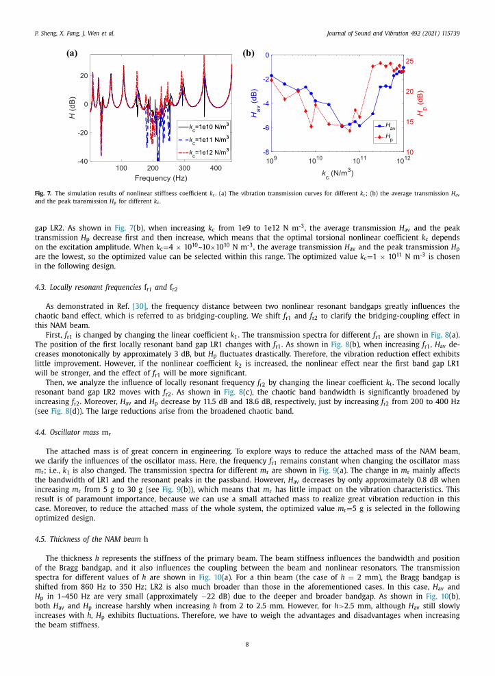
Then, we analyze the influence of the nonlinear coefficient k c in torsional motion. The transmission spectra for different
values of k c are shown in Fig. 7 (a). It can be seen that k c mainly affects the vibration resonances near the second band
7
P. Sheng, X. Fang, J. Wen et al. Journal of Sound and Vibration 492 (2021) 115739
Fig. 7. The simulation results of nonlinear stiffness coefficient k c . (a) The vibration transmission curves for different k c ; (b) the average transmission H av
and the peak transmission H p for different k c .
gap LR2. As shown in Fig. 7 (b), when increasing k c from 1e9 to 1e12 N m
-3 , the average transmission H av and the peak
transmission H p decrease first and then increase, which means that the optimal torsional nonlinear coefficient k c depends
on the excitation amplitude. When k c = 4 × 10 10 ~10 ×10 10 N m
-3 , the average transmission H av and the peak transmission H p
are the lowest, so the optimized value can be selected within this range. The optimized value k c = 1 × 10 11 N m
-3 is chosen
in the following design.
4.3. Locally resonant frequencies f r1 and f r2
As demonstrated in Ref. [30] , the frequency distance between two nonlinear resonant bandgaps greatly influences the
chaotic band effect, which is referred to as bridging-coupling. We shift f r1 and f r2 to clarify the bridging-coupling effect in
this NAM beam.
First, f r1 is changed by changing the linear coefficient k 1 . The transmission spectra for different f r1 are shown in Fig. 8 (a).
The position of the first locally resonant band gap LR1 changes with f r1 . As shown in Fig. 8 (b), when increasing f r1 , H av de-
creases monotonically by approximately 3 dB, but H p fluctuates drastically. Therefore, the vibration reduction effect exhibits
little improvement. However, if the nonlinear coefficient k 2 is increased, the nonlinear effect near the first band gap LR1
will be stronger, and the effect of f r1 will be more significant.
Then, we analyze the influence of locally resonant frequency f r2 by changing the linear coefficient k t . The second locally
resonant band gap LR2 moves with f r2 . As shown in Fig. 8 (c), the chaotic band bandwidth is significantly broadened by
increasing f r2 . Moreover, H av and H p decrease by 11.5 dB and 18.6 dB, respectively, just by increasing f r2 from 200 to 400 Hz
(see Fig. 8 (d)). The large reductions arise from the broadened chaotic band.
4.4. Oscillator mass m r
The attached mass is of great concern in engineering. To explore ways to reduce the attached mass of the NAM beam,
we clarify the influences of the oscillator mass. Here, the frequency f r1 remains constant when changing the oscillator mass
m r ; i.e., k 1 is also changed. The transmission spectra for different m r are shown in Fig. 9 (a). The change in m r mainly affects
the bandwidth of LR1 and the resonant peaks in the passband. However, H av decreases by only approximately 0.8 dB when
increasing m r from 5 g to 30 g (see Fig. 9 (b)), which means that m r has little impact on the vibration characteristics. This
result is of paramount importance, because we can use a small attached mass to realize great vibration reduction in this
case. Moreover, to reduce the attached mass of the whole system, the optimized value m r = 5 g is selected in the following
optimized design.
4.5. Thickness of the NAM beam h
The thickness h represents the stiffness of the primary beam. The beam stiffness influences the bandwidth and position
of the Bragg bandgap, and it also influences the coupling between the beam and nonlinear resonators. The transmission
spectra for different values of h are shown in Fig. 10 (a). For a thin beam (the case of h = 2 mm), the Bragg bandgap is
shifted from 860 Hz to 350 Hz; LR2 is also much broader than those in the aforementioned cases. In this case, H av and
H p in 1~450 Hz are very small (approximately −22 dB) due to the deeper and broader bandgap. As shown in Fig. 10 (b),
both H av and H p increase harshly when increasing h from 2 to 2.5 mm. However, for h > 2.5 mm, although H av still slowly
increases with h, H p exhibits fluctuations. Therefore, we have to weigh the advantages and disadvantages when increasing
the beam stiffness.
8
P. Sheng, X. Fang, J. Wen et al. Journal of Sound and Vibration 492 (2021) 115739
Fig. 8. The simulation results of locally resonant frequencies. (a) The vibration transmission curves for different f r1 ; (b) the average transmission H av and
the peak transmission H p for different f r1 ; (c) the vibration transmission curves for different f r2 ; (d) the average transmission H av and the peak transmission
H p for different f r2 .
Fig. 9. The simulation results of oscillator mass m r . (a) The vibration transmission curves for different m r ; (b) the average transmission H av and the peak
transmission H p for different m r .
4.6. Comparing by synthesis
To compare the vibration reduction characteristics of various parameters of the NAM beam, the reductions of the av-
erage transmission H av for different parameters are shown in Fig. 11 . The varying ranges of the different parameters are
labeled in the rectangles. It is found that the vibration transmission of the NAM beam is insensitive to the attached mass,
which is helpful in reducing the weight of the structure. In addition, the vibration transmission is sensitive to the excitation
amplitude, locally resonant frequency f r2 and nonlinear stiffness coefficients, especially f r2 . Therefore, by optimizing these
parameters, the vibration reduction performance can be manipulated.
9
P. Sheng, X. Fang, J. Wen et al. Journal of Sound and Vibration 492 (2021) 115739
Fig. 10. The simulation results of beam thickness h . (a) The vibration transmission curves for different h ; (b) the average transmission H av and the peak
transmission H p for different h .
Fig. 11. Comparison of the reductions of the average transmission H av for different parameters.
Table 2
The mass ratio of the initial model and optimized model.
Different model Initial NAM beam Optimized NAM beam
Mass ratio (%) 56.2% 28.1%
5. Optimized design
According to the above analyses, we optimize the NAM beam by choosing proper parameter values and realize it in
experiment. The initial parameters are m r = 10 g, f r2 = 225 Hz, k 2 = 3.276e6 N m
-3 , and k c = 1e10 N m
-3 . Considering the exper-
imental realization, the optimized parameters are m r = 5 g, f r2 = 320 Hz, k 2 = 3.276e8 N m
-3 , and k c = 1e11 N m
-3 . The other
parameters are listed in Table 1 . Table 2 shows the mass ratio between the attached mass of the locally resonant unit cell
and the primary beam. Compared with the initial parameters, the mass ratio of the optimized parameters is reduced by half.
As present in Refs [7 , 38] , many linear acoustic metamaterials use more than 100% attached mass ratio to realize broadband
reduction. This paper reduces the attached mass from 56.2% to 28.1%, which is meaningful in practice. Furthermore, because
the chaotic band effect is insensitive to the attached mass, it is possible to reach a larger reduction with more elaborate
resonators.
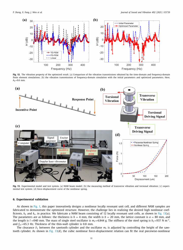
The vibration transmission spectra of the optimized result are shown in Fig. 12 (a). Both the time-domain and frequency-
domain solutions are provided, which are consistent except for two peaks at 58 Hz and 94 Hz. Comparing the responses
of the linear and nonlinear metamaterial beam, it is obvious that nonlinearity significantly reduced the resonant peak at
30~450 Hz by 15 dB.
Moreover, great differences in the transmissions between the initial and optimized design are illustrated in Fig. 12 (b).
With the optimized parameters, the vibration transmission in the concerned frequency range is significantly reduced, at-
tributing to the enhanced the chaotic band effect in optimized design. Therefore, the optimized NAM beam achieves low-
frequency, broadband, and highly efficient vibration reduction with a lightweight attachment.
10
P. Sheng, X. Fang, J. Wen et al. Journal of Sound and Vibration 492 (2021) 115739
Fig. 12. The vibration property of the optimized result. (a) Comparison of the vibration transmissions obtained by the time-domain and frequency-domain
finite element simulations; (b) the vibration transmissions of frequency-domain simulation with the initial parameters and optimized parameters. Here,
A 0 = 0.6 mm.
Fig. 13. Experimental model and test system. (a) NAM beam model; (b) the measuring method of transverse vibration and torsional vibration; (c) experi-
mental test system; (d) force-displacement curve of the nonlinear spring.
6. Experimental validation
As shown in Fig. 1 , this paper innovatively designs a nonlinear locally resonant unit cell, and different NAM samples are
fabricated to demonstrate the optimized structure. However, the challenge lies in realizing the desired high nonlinear coef-
ficients, k 2 and k c , in practice. We fabricate a NAM beam consisting of 12 locally resonant unit cells, as shown in Fig. 13 (a).
The parameters are as follows: the thickness is h = 4 mm, the width is b = 20 mm, the lattice constant is a = 80 mm, and
the length is l = 040 mm. The mass of single steel oscillator is m r = 4.844 g. The stiffness of the steel spring is k 1 = 937 N m
-1 ,
and f r1 = 65.3 Hz. Thickness of the thin-wall cylinder is 0.8 mm.
The clearance δ1 between the sawtooth cylinder and the oscillator m r is adjusted by controlling the height of the saw-
tooth cylinder. As shown in Fig. 13 (d), the cubic nonlinear force-displacement relation can fit the real piecewise-nonlinear
11
P. Sheng, X. Fang, J. Wen et al. Journal of Sound and Vibration 492 (2021) 115739
Fig. 14. Natural frequency test results. (a) Transverse motion vibration transmission; (b) torsional motion vibration transmission.
Fig. 15. Experimental results of a single oscillator. (a) Vibration transmission curves of the linear beam; (b) comparison of the linear and nonlinear vibration
transmission curves.
curve well, which confirms the approximate method adopted in Section 2 . A clearance δ2 between the cylindrical support
and the oscillator m r is designed to be 0.15 mm.
The experimental system consists of a laser vibrometer, an actuator and a signal generator ( Fig. 13 (c)). The driving signal
is white noise. The driving level (i.e., the input amplitude), is controlled by the voltage of the amplifier. The excitation
spectra under different voltage are shown in Appendix C . The input amplitudes of amplifier are 2.8 mm s -1 , 8 mm s -1 and
13.3 mm s -1 for levels L1, L2 and L3, respectively.
First, the transverse vibration and torsional vibration of the locally resonant unit cell are measured by the laser vibrom-
eter. The measuring method is shown in Fig. 13 (b). The transmissions of the transverse and torsional vibrations are shown
in Fig. 14 . Increasing the driving level can shift the natural frequency of the transverse vibration from 100 Hz to 70 Hz, and
can slightly reduce resonant frequencies and transmissions of torsional vibration (from 370 to 350 Hz).
For the beam, the excitation is applied at the left end of the NAM beam. The other positions of the beam are free. The
vibration amplitudes of the left end and right end of the NAM beam are measured by the laser vibrometer to derive the
transmission.
Firstly, we obtain a linearized metamaterial as reference by enlarging the clearance δ1 to 1 mm and enlarging δ2 to
0.5 mm (slightly increasing the radius of the oscillator’s inner hole). The clearance δ1 far exceeds the maximum vibration
amplitude of the oscillator, so that k n = 0. The clearance δ2 is also large that leads to k c → 0. This measurement makes non-
linearity negligible, i.e., a linear beam. The transmissions of this linear beam under different driving levels are shown in
Fig. 15 (a). The transmission spectra nearly remain constant when improving the driving amplitude.
Then, we set δ1 = 0.1 mm and δ2 = 0.15 mm to produce the two sources of clearance nonlinearity. The vibration trans-
missions of the nonlinear beam under different driving levels are shown in Fig. 15 (b). By increasing the driving levels, the
vibration reduction effect between the two locally resonant band gaps becomes more obvious. The NAM beam has a strongly
nonlinear effect in the range of 90–500 Hz, so it can obviously suppress the resonances.
Furthermore, we double the oscillator mass m r and conduct the same experiments above. As shown in Fig. 16 , the low-
frequency vibration reduction becomes greater for higher driving level. The NAM beam presents a strongly nonlinear effect
in 70–600 Hz to suppress the resonances.
12
P. Sheng, X. Fang, J. Wen et al. Journal of Sound and Vibration 492 (2021) 115739
Fig. 16. Comparison of the linear and nonlinear vibration transmission curves of the two oscillators.
Fig. 17. Time-domain responses under a single-frequency sinusoidal excitation ( f = 127.5 Hz). (a) Time-domain signal: driving amplitude L1 (1 mm s -1 );
(b) the phase diagrams and maximal Lyapunov exponent: driving amplitude L1; (c) time-domain signal: driving amplitude L2 (13.3 mm s -1 ); (d) the phase
diagrams and maximal Lyapunov exponent: driving amplitude L2.
To confirm the chaotic property in experiment, we analyze the characters of the time-domain response signals under
small (1 mm s -1 ) and large (13.3 mm s -1 ) driving amplitudes. The experiment is conducted on the nonlinear metamaterial
beam with m r = 4.844 g. A resonant frequency 127.5 Hz near the first bandgap is chosen for example. In this case, the
standard sinusoidal signal is applied at the left end of the NAM beam, and the time-domain waveform of velocity at the
right end is measured. As shown in Fig. 17 (a)(b), the phase diagram and the response under the small driving amplitude
L1 approximates to a quasi-periodic signal. In contrast, the highly irregular phase diagram and the large Lyapunov exponent
4.796 in Fig. 17 (c)(d) indicate that the response under large driving amplitude L2 is strongly chaotic.
13
P. Sheng, X. Fang, J. Wen et al. Journal of Sound and Vibration 492 (2021) 115739
Fig. 18. The varying trends of the transmission for different driving amplitudes of amplifier (sinusoidal excitation of f = 127.5 Hz).
Finally, we measure the varying trends of the transmission this resonance when increasing the driving amplitude. As
shown in Fig. 18 , the transmissions obtained from the time-domain amplitude and frequency-domain peak component are
consistent. As the driving amplitude increases, the nonlinear effect becomes stronger, and the transmission decreases. This
trend also agrees with the theoretical analysis in Section 4.1 .
7. Conclusions
This paper studies a finite NAM beam model including a bridging-coupling locally resonant unit cell. Both time-domain
and frequency-domain finite element models are established to calculate the vibration characteristics. We systematically
analyze the influences of various parameters on the bandwidth and efficiency of vibration reduction. It is found that the
vibration transmission of the NAM beam is insensitive to the attached mass, which is helpful for reducing the weight of
resonators. Moreover, increasing the second locally resonant frequency, excitation amplitude and nonlinear stiffness coeffi-
cients can enhance the nonlinear effects and significantly broaden the chaotic band bandwidth. According to the parameter
manipulation trends, we optimize the NAM beam to realize the low-frequency, broadband, and highly efficient vibration
reduction with only 28.1% attached mass. The lightweight attached mass is much smaller than the original NAM beam. Fi-
nally, we fabricate a strongly nonlinear metamaterial beam based on the optimized parameters. Both frequency-domain and
time-domain experiments validate the optimized NAM structure and chaotic properties.
This work highlights important varying trends of the vibration transmission of the NAM structure when changing 6
representative parameters. These results are useful to conceive new NAM structures. The optimized design shows the great
potential of NAMs for the realization of low-frequency and broadband vibration reduction with only small attachments,
which is preferable in broad applications.
Declaration of Competing Interest
None.
Acknowledgments
This research was funded by the National Natural Science Foundation of China (Project nos. 12002371 , 11991032 and
11991034 ).
Appendix A. Finite element method
For the NAM beam model described in Section 2 , the FD-FEM and TD-FEM are used for the simulation to analyze the
low-frequency vibration characteristics.
A1. Frequency-domain finite element method
For the transformed motion equation of Eq. (10) , the frequency-domain solution can be derived with the harmonic bal-
ance method, which has been widely used in nonlinear dynamics such as the research in [31] . After obtaining the dis-
placement response of the beam, the vibration transmission H defined by Eq. (5) is obtained. The values of the NAM beam
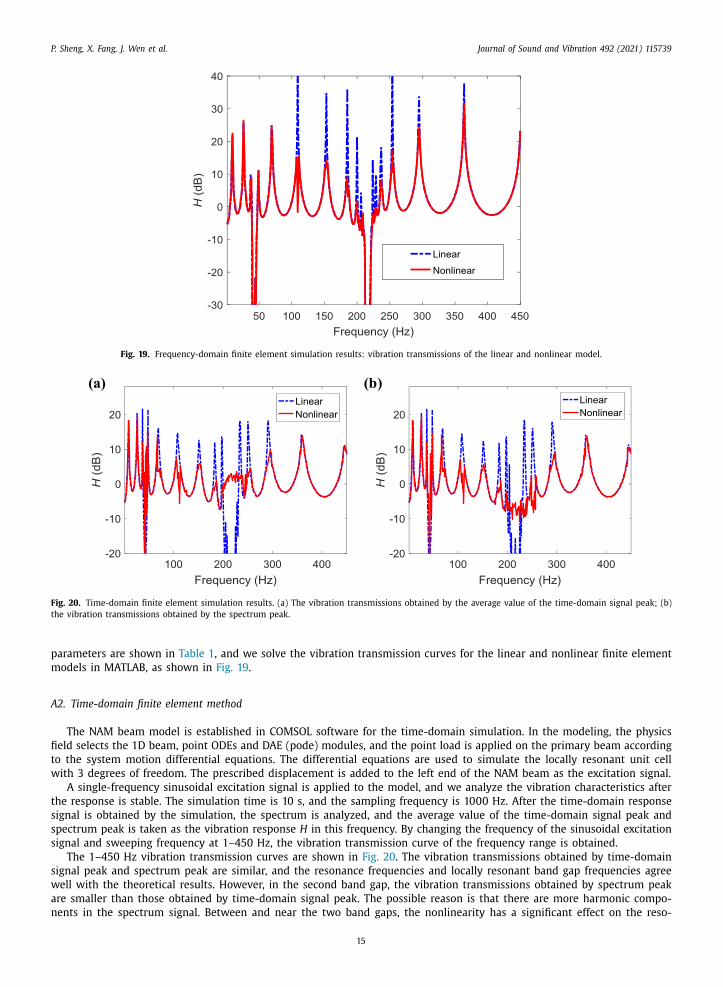
P. Sheng, X. Fang, J. Wen et al. Journal of Sound and Vibration 492 (2021) 115739
Fig. 19. Frequency-domain finite element simulation results: vibration transmissions of the linear and nonlinear model.
Fig. 20. Time-domain finite element simulation results. (a) The vibration transmissions obtained by the average value of the time-domain signal peak; (b)
the vibration transmissions obtained by the spectrum peak.
parameters are shown in Table 1 , and we solve the vibration transmission curves for the linear and nonlinear finite element
models in MATLAB, as shown in Fig. 19 .
A2. Time-domain finite element method
The NAM beam model is established in COMSOL software for the time-domain simulation. In the modeling, the physics
field selects the 1D beam, point ODEs and DAE (pode) modules, and the point load is applied on the primary beam according
to the system motion differential equations. The differential equations are used to simulate the locally resonant unit cell
with 3 degrees of freedom. The prescribed displacement is added to the left end of the NAM beam as the excitation signal.
A single-frequency sinusoidal excitation signal is applied to the model, and we analyze the vibration characteristics after
the response is stable. The simulation time is 10 s, and the sampling frequency is 10 0 0 Hz. After the time-domain response
signal is obtained by the simulation, the spectrum is analyzed, and the average value of the time-domain signal peak and
spectrum peak is taken as the vibration response H in this frequency. By changing the frequency of the sinusoidal excitation
signal and sweeping frequency at 1–450 Hz, the vibration transmission curve of the frequency range is obtained.
The 1–450 Hz vibration transmission curves are shown in Fig. 20 . The vibration transmissions obtained by time-domain
signal peak and spectrum peak are similar, and the resonance frequencies and locally resonant band gap frequencies agree
well with the theoretical results. However, in the second band gap, the vibration transmissions obtained by spectrum peak
are smaller than those obtained by time-domain signal peak. The possible reason is that there are more harmonic compo-
nents in the spectrum signal. Between and near the two band gaps, the nonlinearity has a significant effect on the reso-
15
P. Sheng, X. Fang, J. Wen et al. Journal of Sound and Vibration 492 (2021) 115739
Fig. 21. The excitation spectra under different driving level, where the driving level L1: the driving voltage of amplifier is 1 V; the driving level L2: the
driving voltage of amplifier is 3 V; the driving level L3: the driving voltage of amplifier is 5 V.
nances, so this method can better describe the model in this paper. The time-domain simulation in the band gap position
of the linear model is unstable at some frequencies, but this does not affect the analysis of the vibration characteristics.
Appendix B. Finite element matrix
B1. Beam element
M s , C s and K s denote the mass matrix, damping matrix and stiffness matrix of beam element, respectively. Without
considering the geometric nonlinearity and inertial nonlinearity of the primary beam, the finite element matrices for the
flexural vibration of the beam are
M s =
ρlhb
420
⎡
⎢ ⎣
156 22 l 54 −13 l
22 l 4 l 2 13 l −3 l 2
54 13 l 156 −22 l 2
−13 l −3 l 2 −22 l 4 l 2
⎤
⎥ ⎦
K s =
EI
l 3
⎡
⎢ ⎣
12 6 l −12 6 l
6 l 4 l 2 −6 l 2 l 2
−12 −6 l 12 −6 l
6 l 2 l 2 −6 l 4 l 2
⎤
⎥ ⎦
C s = c 0 K s
where c 0 = 0.001/(2 π f ), l = a /2, I = bh 3 /12, and f denotes the driving frequency.
B2. Locally resonant unit cell
M e , C e , K e and N e denote the mass matrix, damping matrix, stiffness matrix and nonlinear stiffness matrix of the locally
resonant unit cell, respectively. The finite element matrices of the locally resonant unit cell are
M e =
⎡
⎢ ⎢ ⎣
m r 0 0 m r 0
0 J r 0 0 0
0 m r l r m r 0 0
0 0 0 m 0 0
0 0 0 0 J 0
⎤
⎥ ⎥ ⎦
K e =
⎡
⎢ ⎢ ⎣
k 1 0 0 0 0
0 k t −k 3 l r 0 −k t 0 0 k 3 0 0
−k 1 0 0 0 0
0 −k t 0 0 k t
⎤
⎥ ⎥ ⎦
N e =
⎡
⎢ ⎢ ⎣
k 2 0 0 0 0
0 0 −k c l r 0 0
0 0 k c 0 0
−k 2 0 0 0 0
0 0 0 0 0
⎤
⎥ ⎥ ⎦
C e =
⎡
⎢ ⎢ ⎣
c 0 0 0 0
0 0 0 0 0
0 0 0 0 0
−c 0 0 0 0
0 0 0 0 0
⎤
⎥ ⎥ ⎦
Appendix C. Excitation spectrum
The excitation spectra as a reference value under different driving level are shown in Fig. 21 .
References
[1] S.A. Cummer, J. Christensen, A. Alù, Controlling sound with acoustic metamaterials, Nat. Rev. Mater. 1 (2016) 16001 https://doi.org/, doi: 10.1038/natrevmats.2016.1 .
[2] K.Y. Bliokh, F. Nori, Transverse spin and surface waves in acoustic metamaterials, Phys. Rev. B 99 (2019) 020301 https://doi.org/, doi: 10.1103/PhysRevB.99.020301 .
P. Sheng, X. Fang, J. Wen et al. Journal of Sound and Vibration 492 (2021) 115739
[3] Z. Liu, X. Zhang, Y. Mao, Y. Zhu, Z. Yang, C. Chan, P. Sheng, Locally resonant sonic materials, Science 289 (20 0 0) 1734–1736 https://doi.org/, doi: 10.1126/science.289.5485.1734 .
[4] G. Ma, P. Sheng, Acoustic metamaterials: from local resonances to broad horizons, Sci. Adv. 2 (2016) e1501595 https://doi.org/, doi: 10.1126/sciadv.1501595 .
[5] G. Ma, M. Yang, S. Xiao, Z. Yang, P. Sheng, Acoustic metasurface with hybrid resonances, Nat. Mater. 13 (2014) 873–878 https://doi.org/, doi: 10.1038/NMAT3994 .
[6] J. Zhao, B. Bonello, O. Boyko, Focusing of the lowest-order antisymmetric Lamb mode behind a gradient-index acoustic metalens with local resonators,
Phys. Rev. B 93 (2016) 174306 https://doi.org/, doi: 10.1103/PhysRevB.93.174306 . [7] M.I. Hussein, M.J. Leamy, M. Ruzzene, Dynamics of phononic materials and structures: historical origins, recent progress, and future outlook, Appl.
Mech. Rev. 66 (2014) 040802 https://doi.org/, doi: 10.1115/1.4026911 . [8] H. Zhang, Y. Xiao, J. Wen, D. Yu, X. Wen, Ultra-thin smart acoustic metasurface for low-frequency sound insulation, Appl. Phys. Lett. 108 (2016) 141902
https://doi.org/, doi: 10.1063/1.4945664 . [9] Z. Lu, L. Cai, J. Wen, X. Chen, Physically realizable broadband acoustic metamaterials with anisotropic density, Chin. Phys. Lett. 36 (2019) 24301
https://doi.org/, doi: 10.1088/0256-307X/36/2/024301 . [10] N. Higashiyama, Y. Doi, A. Nakatani, Nonlinear dynamics of a model of acoustic metamaterials with local resonators, Nonlinear Theory Applica. 8
[11] L. Cveticanin, M. Zukovic, Negative effective mass in acoustic metamaterial with nonlinear mass-in-mass subsystems, Commun. Nonlinear Sci. Numer. Simul. 51 (2017) 89–104 https://doi.org/, doi: 10.1016/j.cnsns.2017.03.017 .
[12] T. Dauxois, Fermi, Pasta, Ulam, and a mysterious lady, Phys. Today 61 (2008) https://doi.org/, doi: 10.1063/1.2835154 . [13] W. Zhou, X. Li, Y. Wang, W. Chen, G. Huang, Spectro-spatial analysis of wave packet propagation in nonlinear acoustic metamaterials, J. Sound Vib. 413
(2018) 250–269 https://doi.org/, doi: 10.1016/j.jsv.2017.10.023 . [14] A .F. Vakakis, M.A . AL-Shudeifat, M.A . Hasan, Interactions of propagating waves in a one-dimensional chain of linear oscillators with a strongly nonlinear
[15] L. Bonanomi, G. Theocharis, C. Daraio, Wave propagation in granular chains with local resonances, Phys. Rev. E 91 (2015) 033208 https://doi.org/,doi: 10.1103/PhysRevE.91.033208 .
[16] P.B. Silva, M.J. Leamy, M. Geers, V.G. Kouznetsova, Emergent subharmonic band gaps in nonlinear locally resonant metamaterials induced by autopara-metric resonance, Phys. Rev. E 99 (2019) 063003 https://doi.org/, doi: 10.1103/PhysRevE.99.063003 .
[17] M.D. Fronk, M.J. Leamy, Higher-order dispersion stability, and waveform invariance in nonlinear monoatomic and diatomic systems, J. Vib. Acoust. 139 (2017) 051003 https://doi.org/, doi: 10.1115/1.4036501 .
[18] K. Manktelow, R.K. Narisetti, M.J. Leamy, M. Ruzzene, Finite-element based perturbation analysis of wave propagation in nonlinear periodic structures,
Mech. Syst. Signal Process. 39 (2013) 32–46 https://doi.org/, doi: 10.1016/j.ymssp.2012.04.015 . [19] R. Khajehtourian, M.I. Hussein, Damping and nonlinearity in elastic metamaterials: treatment and effects, AIP Adv. 4 (2014) 124308 https://doi.org/,
doi: 10.1121/1.4877386 . [20] O.R. Bilal, A. Foehr, C. Daraio, Bistable metamaterial for switching and cascading elastic vibrations, Proc. Natl. Acad. Sci. 114 (2017) 4603–4606
https://doi.org/, doi: 10.1073/pnas.1618314114 . [21] D. Hatanaka, T. Darras, I. Mahboob, K. Onomitsu, H. Yamaguchi, Broadband reconfigurable logic gates in phonon waveguides, Sci. Rep. 7 (2017) 12745
[22] F. Li, P. Anzel, J. Yang, P.G. Kevrekidis, C. Daraio, Granular acoustic switches and logic elements, Nat. Commun. 5 (2014) 5311 https://doi.org/, doi: 10.1038/ncomms6311 .
[23] X. Fang, J. Wen, B. Bonello, J. Yin, D. Yu, Ultra-low and ultra-broad-band nonlinear acoustic metamaterials, Nat. Commun. 8 (2017) 1288 https://doi.org/,doi: 10.1038/s41467- 017- 00671- 9 .
[24] X. Fang, J. Wen, H. Benisty, D. Yu, Ultrabroad acoustical limiting in nonlinear metamaterials due to adaptive-broadening band-gap effect, Phys. Rev. B101 (2020) 104304 https://doi.org/, doi: 10.1103/PhysRevB.101.104304 .
[25] P.F. Pai, H. Peng, S. Jiang, Acoustic metamaterial beams based on multi-frequency vibration absorbers, Int. J. Mech. Sci. 79 (2014) 195–205
https://doi.org/, doi: 10.1016/j.ijmecsci.2013.12.013 . [26] V. Romero-García, A. Krynkin, L.M. Garcia-Raffi, O. Umnova, J.V. Sánchez-Pérez, Multi-resonant scatterers in sonic crystals: locally multi-resonant
acoustic metamaterial, J. Sound Vib. 332 (2013) 184–198 https://doi.org/, doi: 10.1016/j.jsv.2012.08.003 . [27] A. Luongo, D. Zulli, Dynamic analysis of externally excited NES-controlled systems via a mixed Multiple Scale/Harmonic Balance algorithm, Nonlinear
Dyn. 70 (2012) 2049–2061 https://doi.org/, doi: 10.1007/s11071- 012- 0597- 6 . [28] T.F. van Nuland, P.B. Silva, A. Sridhar, M.G. Geers, V.G. Kouznetsova, Transient analysis of nonlinear locally resonant metamaterials via computational
[29] X. Fang, J. Wen, B. Bonello, J. Yin, D. Yu, Wave propagation in one-dimensional nonlinear acoustic metamaterials, New J. Phys. 19 (2017) 053007https://doi.org/, doi: 10.1088/1367-2630/aa6d49 .
[30] X. Fang, J. Wen, D. Yu, J. Yin, Bridging-Coupling band gaps in nonlinear acoustic metamaterials, Phys. Rev. Appl. 10 (2018) 054049 https://doi.org/,doi: 10.1103/PhysRevApplied.10.054049 .
[31] X. Fang, J. Wen, J. Yin, D. Yu, Y. Xiao, Broadband and tunable one-dimensional strongly nonlinear acoustic metamaterials: theoretical study, Phys. Rev.E 94 (2016) 052206 https://doi.org/, doi: 10.1103/PhysRevE.94.052206 .
[32] X. Fang, J. Wen, J. Yin, D. Yu, Wave propagation in nonlinear metamaterial multi-atomic chains based on homotopy method, AIP Adv. 6 (2016) 121706https://doi.org/, doi: 10.1063/1.4971761 .
[33] B.S. Lazarov, J.S. Jensen, Low-frequency band gaps in chains with attached non-linear oscillators, Int. J. Non Linear Mech. 42 (2007) 1186–1193
https://doi.org/, doi: 10.1016/j.ijnonlinmec.20 07.09.0 07 . [34] H. Kantz, A robust method to estimate the maximal Lyapunov exponent of a time series, Phys. Lett. A 185 (1994) 77–87 https://doi.org/, doi: 10.1016/
0375-9601(94)90991-1 . [35] J. Eckmann, S.O. Kamphorst, D. Ruelle, S. Ciliberto, Liapunov exponents from time series, Phys. Rev. A 34 (1986) 4 971–4 979 https://doi.org/, doi: 10.
1103/PhysRevA.34.4971 . [36] C. Daraio, V.F. Nesterenko, E. Herbold, S. Jin, Tunability of solitary wave properties in one-dimensional strongly nonlinear phononic crystals, Phys. Rev.
E 73 (2006) 026610 https://doi.org/, doi: 10.1103/PhysRevE.73.026610 .
[37] J. Lydon, G. Theocharis, C. Daraio, Nonlinear resonances and energy transfer in finite granular chains, Phys. Rev. E 91 (2015) 023208 https://doi.org/,doi: 10.1103/PhysRevE.91.023208 .
[38] Y. Xiao, J. Wen, G. Wang, X. Wen, Theoretical and experimental study of locally resonant and Bragg band gaps in flexural beams carrying periodicarrays of beam-like resonators, J. Vib. Acoust. 135 (2013) 041006 https://doi.org/, doi: 10.1115/1.4024214 .