Seismic structure of the crust and uppermost mantle of South America and surrounding oceanic basins Gary S. Chulick a , Shane Detweiler b, * , Walter D. Mooney b a Mt. Aloysius College, 7373 Admiral Peary Hwy, Cresson, PA 16630, USA b United States Geological Survey, MS 977, 345 Middlefield Road, Menlo Park, CA 94025, USA article info Article history: Received 19 July 2011 Accepted 5 June 2012 Keywords: Crustal structure Seismic velocity South America abstract We present a new set of contour maps of the seismic structure of South America and the surrounding ocean basins. These maps include new data, helping to constrain crustal thickness, whole-crustal average P-wave and S-wave velocity, and the seismic velocity of the uppermost mantle (P n and S n ). We find that: (1) The weighted average thickness of the crust under South America is 38.17 km (standard deviation, s.d. 8.7 km), which is w1 km thinner than the global average of 39.2 km (s.d. 8.5 km) for continental crust. (2) Histograms of whole-crustal P-wave velocities for the South American crust are bi-modal, with the lower peak occurring for crust that appears to be missing a high-velocity (6.9e7.3 km/s) lower crustal layer. (3) The average P-wave velocity of the crystalline crust (P cc ) is 6.47 km/s (s.d. 0.25 km/s). This is essentially identical to the global average of 6.45 km/s. (4) The average P n velocity beneath South America is 8.00 km/s (s.d. 0.23 km/s), slightly lower than the global average of 8.07 km/s. (5) A region across northern Chile and northeast Argentina has anomalously low P- and S-wave velocities in the crust. Geographically, this corresponds to the shallowly-subducted portion of the Nazca plate (the Pampean flat slab first described by Isacks et al., 1968), which is also a region of crustal extension. (6) The thick crust of the Brazilian craton appears to extend into Venezuela and Colombia. (7) The crust in the Amazon basin and along the western edge of the Brazilian craton may be thinned by extension. (8) The average crustal P-wave velocity under the eastern Pacific seafloor is higher than under the western Atlantic seafloor, most likely due to the thicker sediment layer on the older Atlantic seafloor. Published by Elsevier Ltd. 1. Introduction The construction of continent-scale maps of geophysical prop- erties provides a broad picture of the structure of the Earth. For example, a map of crustal thickness indicates the lateral extent of tectonic provinces such as highly extended regions and orogenic zones. Likewise, maps of crustal seismic velocities can help to delineate platforms, shields, sedimentary basins, and exotic accreted terrains (Christensen and Mooney, 1995). Geophysical maps provide a means of identifying crustal properties that delin- eate geologic provinces (e.g., Prodehl, 1984; Meissner, 1986; Collins, 1988; Pakiser and Mooney, 1989; Blundell et al., 1992; Pavlenkova, 1996; Yuan, 1996; Chulick and Mooney, 2002; Fuck et al., 2008; Cordani et al., 2009; Cordani et al., 2010). We present the first set of contour maps based on seismic- refraction work combined with other forms of seismic data (i.e., seismic reflection, sonobuoy, receiver function and earthquake models) for the entire continent of South America and the surrounding ocean basins. There are several reasons why new maps are warranted at this time. First, the quantity and quality of data on South American crustal structure has grown substantially in the past decade or so, with new seismic surveys (e.g. Wigger et al.,1994; Flueh et al.,1998; Patzwahl et al.,1999; Bohm et al., 2002; ANCORP Working Group, 2003; Berrocal et al., 2004; Schmitz et al., 2005; Rodger et al., 2006; Scherwath et al., 2006; Soares et al., 2006; Greenroyd et al., 2007) conducted that cover hitherto unexplored regions (e.g. the Chilean Andes and Amazonia) as well as provide better resolution in previously studied areas (e.g., the Peruvian Andes, and eastern Brazil). However, this work in South America has generally not been done at the continental scale and frequently depends on passive source data (e.g. Schmitz et al., 1999; Assumpção et al., 2002, 2004; An and Assumpção, 2005; Tavera et al., 2006; Lange et al., 2007; Heit et al., 2008; Wölbern et al., 2009). This study consolidates the * Corresponding author. Tel.: þ1 650 329 5192; fax: þ1 650 329 5163. E-mail address: [email protected](S. Detweiler). Contents lists available at SciVerse ScienceDirect Journal of South American Earth Sciences journal homepage: www.elsevier.com/locate/jsames Journal of South American Earth Sciences 42 (2013) 260e276 0895-9811/$ e see front matter Published by Elsevier Ltd. http://dx.doi.org/10.1016/j.jsames.2012.06.002
Transcript
at SciVerse ScienceDirect
Journal of South American Earth Sciences 42 (2013) 260e276
Seismic structure of the crust and uppermost mantle of South Americaand surrounding oceanic basins
Gary S. Chulick a, Shane Detweiler b,*, Walter D. Mooney b
aMt. Aloysius College, 7373 Admiral Peary Hwy, Cresson, PA 16630, USAbUnited States Geological Survey, MS 977, 345 Middlefield Road, Menlo Park, CA 94025, USA
a r t i c l e i n f o
Article history:Received 19 July 2011Accepted 5 June 2012
Keywords:Crustal structureSeismic velocitySouth America
0895-9811/$ e see front matter Published by Elseviehttp://dx.doi.org/10.1016/j.jsames.2012.06.002
a b s t r a c t
We present a new set of contour maps of the seismic structure of South America and the surroundingocean basins. These maps include new data, helping to constrain crustal thickness, whole-crustal averageP-wave and S-wave velocity, and the seismic velocity of the uppermost mantle (Pn and Sn). We find that:(1) The weighted average thickness of the crust under South America is 38.17 km (standard deviation,s.d. �8.7 km), which is w1 km thinner than the global average of 39.2 km (s.d. �8.5 km) for continentalcrust. (2) Histograms of whole-crustal P-wave velocities for the South American crust are bi-modal, withthe lower peak occurring for crust that appears to be missing a high-velocity (6.9e7.3 km/s) lower crustallayer. (3) The average P-wave velocity of the crystalline crust (Pcc) is 6.47 km/s (s.d. �0.25 km/s). This isessentially identical to the global average of 6.45 km/s. (4) The average Pn velocity beneath SouthAmerica is 8.00 km/s (s.d. �0.23 km/s), slightly lower than the global average of 8.07 km/s. (5) A regionacross northern Chile and northeast Argentina has anomalously low P- and S-wave velocities in the crust.Geographically, this corresponds to the shallowly-subducted portion of the Nazca plate (the Pampean flatslab first described by Isacks et al., 1968), which is also a region of crustal extension. (6) The thick crust ofthe Brazilian craton appears to extend into Venezuela and Colombia. (7) The crust in the Amazon basinand along the western edge of the Brazilian craton may be thinned by extension. (8) The average crustalP-wave velocity under the eastern Pacific seafloor is higher than under the western Atlantic seafloor,most likely due to the thicker sediment layer on the older Atlantic seafloor.
Published by Elsevier Ltd.
1. Introduction
The construction of continent-scale maps of geophysical prop-erties provides a broad picture of the structure of the Earth. Forexample, a map of crustal thickness indicates the lateral extent oftectonic provinces such as highly extended regions and orogeniczones. Likewise, maps of crustal seismic velocities can help todelineate platforms, shields, sedimentary basins, and exoticaccreted terrains (Christensen and Mooney, 1995). Geophysicalmaps provide a means of identifying crustal properties that delin-eate geologic provinces (e.g., Prodehl, 1984; Meissner, 1986; Collins,1988; Pakiser and Mooney, 1989; Blundell et al., 1992; Pavlenkova,1996; Yuan, 1996; Chulick and Mooney, 2002; Fuck et al., 2008;Cordani et al., 2009; Cordani et al., 2010).
: þ1 650 329 5163.
r Ltd.
We present the first set of contour maps based on seismic-refraction work combined with other forms of seismic data (i.e.,seismic reflection, sonobuoy, receiver function and earthquakemodels) for the entire continent of South America and thesurrounding ocean basins. There are several reasons why newmapsare warranted at this time. First, the quantity and quality of data onSouth American crustal structure has grown substantially in the pastdecadeor so,withnewseismic surveys (e.g.Wiggeret al.,1994; Fluehetal.,1998;Patzwahlet al.,1999;Bohmetal., 2002;ANCORPWorkingGroup, 2003; Berrocal et al., 2004; Schmitz et al., 2005; Rodger et al.,2006; Scherwath et al., 2006; Soares et al., 2006; Greenroyd et al.,2007) conducted that cover hitherto unexplored regions (e.g. theChilean Andes and Amazonia) aswell as provide better resolution inpreviously studied areas (e.g., the Peruvian Andes, and easternBrazil). However, this work in South America has generally not beendone at the continental scale and frequently depends on passivesource data (e.g. Schmitz et al., 1999; Assumpção et al., 2002, 2004;An and Assumpção, 2005; Tavera et al., 2006; Lange et al., 2007;Heit et al., 2008; Wölbern et al., 2009). This study consolidates the
G.S. Chulick et al. / Journal of South American Earth Sciences 42 (2013) 260e276 261
work of previous studies by combining different types of crustalstructure data taken from throughout the continent, includingnumerous geological provinces and tectonic regimes. The maingeologic provinces of South America are shown in Fig. 1.
We also present contour maps and statistical analyses of the S-wave velocity of the crust and Moho of South America. Suchpresentations are particularly relevant given the recent publicationof tomographic S-wave velocity maps of the South Americanmantle (e.g. van der Lee et al., 2001, 2002; Feng et al., 2004, 2007).
Our newly-collected data, mentioned above, have been incor-porated into a comprehensive seismic database (website addressprovided at the end of the article). Each data point used in thisstudy consists of a one-dimensional velocity-depth functionextracted from a published crustal model. More than 75% of thedata points were taken from 2D seismic velocity cross sectionsderived from seismic-refraction data. Every effort has beenmade toinclude results published through 2011; however, some importantand/or recently-completed seismic surveys are not fully available.Nonetheless, we can for the first time produce reasonably detailedmaps of P-wave crustal properties for all of South America, as well
Fig. 1. Main Geological Provinces of South America. (
as corresponding generalized maps of S-wave crustal properties.The locations for all seismic data points used in this study areshown in Fig. 2.
The maps presented here include crustal thickness (Hc), averageP-wave velocity of the whole crust (Pc) and of the crystalline crust(Pcc), sub-Moho P-wave velocity (Pn), average S-wave velocity of thewhole crust (Sc) and of the crystalline crust (Scc), and sub-Moho S-wave velocity (Sn). Furthermore we provide a statistical analysis ofthese parameters, as well as of the velocity ratios Pc/Sc, Pcc/Scc, andPn/Sn. We also present several crustal cross-sections through theSouth American continent synthesized from our velocity datacompilation.
2. Previous work
Maps of deep crustal properties for South America based onseismic-refractiondatahavehithertobeen limited inextent,primarilyto local regions of the Andes (e.g. Wigger et al., 1994; Schmitz, 1994;Bohm et al., 2002; ANCORP Working Group, 2003; Alvarado et al.,2005; Gilbert et al., 2006; Alvarado et al., 2007; Yoon et al., 2009)
After Gubanov and Mooney, pers. comm., 2012).
Fig. 2. Location map for the one-dimensional seismic data profiles used in this study. See: http://earthquake.usgs.gov/research/structure/crust/sam.php for details.
G.S. Chulick et al. / Journal of South American Earth Sciences 42 (2013) 260e276262
and the continentalmargins (e.g. Bezada et al., 2008; Christesonet al.,2008; Agudelo et al., 2009; Pavlenkova et al., 2009). Some localmodeling studies using surface waves have also been performed,principally in Brazil (e.g. Nascimento et al., 2002; Assumpção et al.,2002, 2004; An and Assumpção, 2004; Blaich et al., 2008; Juliaet al., 2008) and Argentina (e.g. Schnabel, 2007; Blaich et al., 2009).
The first true continent-scalemaps of crustal thickness, and sub-Moho S-wave velocities for South America were produced by vander Lee et al. (2001, 2002) and Feng et al. (2004, 2007), usingbody-wave tomography that had been constrained by surfacewaves. Crust 2.0 (Bassin et al., 2000) was done at global scale, butstill contained decent coverage of South America. Here we go onestep further by producing the first continental-scale maps of crustalP-wave and S-wave velocities for South America based ona combination of seismic refraction and reflection surveys, surfacewave analyses, tomography and other forms of seismic data, ina manner analogous to our study of North America (Chulick andMooney, 2002). Thus, for example, our model for the SouthAmerican crustal thickness may be compared to the results of Crust2.0 (Bassin et al., 2000), van der Lee et al. (2001, 2002), and Lloydet al. (2010).
3. Data and uncertainties
We have compiled a catalog of the seismic structure of the crustand uppermost mantle of South America and the surroundingoceans that includes all types of seismic data, including refraction
and reflection profiling, surface-wave and receiver function anal-ysis, and local earthquake tomography (Chulick, 1997). Our SouthAmerican catalog currently contains 889 velocity-depth functions(“data points”), though w25% of these do not reach Moho depths.Of those that do model the entire crust, we have used 658 in thepresent study. About 75% of these utilized velocity-depth functionswere derived from seismic-refraction data. Given the ambiguity inidentifying the thickness of sediments for each individual datapoint, we have adopted a velocity horizon to define the depth of thetop of the crystalline or “consolidated” crust. A P-wave value of 5.8km/s was chosen for this seismic velocity horizon for P-wavefunctions as it is higher than the velocity in most sedimentaryrocks, but lower than the minimum velocity (w5.9 km/s) found invirtually all granitic rocks. Similarly, an S-wave value of 3.35 km/swas chosen as the corresponding velocity horizon for S-wavefunctions.
The accuracy of the generated contour maps is strongly affectedby the uncertainties in the published interpretations of crustalstructure. Useful reviews of the uncertainties associated with themethods utilized to determine the structure of the crust and sub-crustal lithosphere are provided by Mooney (1989) and Bostock(1999). The uncertainties in crustal models arise from suchfactors as the survey method, the spatial resolution of the survey(e.g., the spacing of the shot points and the recording stations), andthe analytical techniques used to process the data. Typically, theuncertainty in the calculated depth of the Moho is approximately5e10%. Thus, a reported crustal thickness of 40 km has an
Table 2Statistical analyses of the crustal and mantle parameters presented in this study.Hc¼ crustal thickness; Pc (Sc)¼ average P-wave (S-wave) velocity of the whole crust(i.e., including sediments); Pcc (Scc)¼ average P-wave (S-wave) velocity of the
G.S. Chulick et al. / Journal of South American Earth Sciences 42 (2013) 260e276 263
uncertainty of �2e4 km. The seismic velocities determined fromrefracted first-arrivals (e.g., Pn) are typically accurate to withina few hundredths of a km/s (Mooney, 1989; Chulick, 1997).
South American geological provinces and place names are pre-sented in Fig. 1, while the locations of the compiled P- and S-wavevelocity-depth functions are shown in Fig. 2. Statistical analyses foreach of the seismic parameters are presented in Tables 1 and 2. Thedata types (seismic refraction, receiver function, etc.) and dataquantity used in the construction of the maps are presented inTable 3. The contour maps presented in Figs. 3e9 were constructedusing commercial software employing the natural-neighbor tech-nique for gridding. Certain regions with very sparse data (e.g., theAmazonas Basin) yielded unreasonable contours. Where possible,we edited these regional results to avoid obvious geographicalerrors, such as oceanic crustal thickness appearing on continentalcrust. The data used are available at the Web address provided atthe end of this article.
4.1. Crustal thickness (Hc)
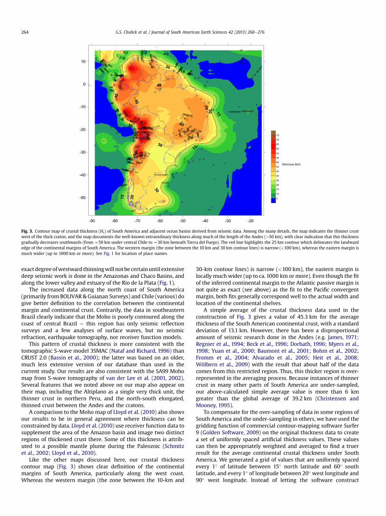
Our map (Fig. 3) demonstrates not only the extraordinarythickness but also the variation found in the continental crustbeneath the Andes. The crust under the central Andes appears toform a single block that is extremely thick, exceeding 60 km fromcentral Peru south through western Bolivia into northern Chile.Since this region corresponds geographically to the Altiplano, weinterpret the Altiplano to be a continental plateau underlain by
Table 1Comparison of statistical analyses of Chulick and Mooney (2002) (North America),Christensen and Mooney (1995) (global), and this study (South America).Hc¼ crustal thickness; Pcc (Scc)¼ average P-wave (S-wave) velocity of the crystallinecrust (i.e., below sediments); Pn (Sn)¼ P-wave (S-wave) velocity of the uppermostmantle. n¼ number of data points; x¼ average value, �s¼ standard deviation. Thestatistical error, �e¼ [sO square root of n].
extremely thick continental crust along a convergent margin. Thissuggests that it is a structural analog to the southern TibetanPlateau.
In central Chile the crust under the Andes is also very thick(>50 km; see Wagner et al., 2005; Heit et al., 2008; Yoon et al.,2009; Lloyd et al., 2010). However, farther south, in the AustralAndes of southern Chile and Patagonia, the crust thins gradually; inthe region of Tierra del Fuego, the crust is only about 30 km thick(Lawrence and Wiens, 2004; Lloyd et al., 2010).
To the north of central Peru, there is far less crustal seismic datathan for areas further to the south (James and Snoke, 1994).However, the seismic refraction surveys and earthquake modelingthat has been done also shows variations in crustal thickness underthe northern Andes (Ocola et al., 1975). In northern Peru, there isevidence that the crust thins to nearly 40 km, but further to thenorth it thickens again to at least 50 km under Colombia andwestern Venezuela (Mooney et al., 1979; Schmitz et al., 2005).
Fig. 3 further indicates a moderately thick (>40 km) crust underthe Guiana and Brazilian Shields (Fig. 1), with clear indications thatthe crust is thinner (w35 km) to the west, under the central part ofthe continent. This moderately thick (w35 km) crust is consistentwith previous studies (e.g. Soares et al., 2006) and has been seenunder other shields as well (e.g. the Canadian Shield (35e50 km),Eaton et al., 2005; the Baltic Shield (35e55 km), Balling, 1995). The
Table 3Distribution of data points for each crustal and uppermost mantle parametermapped in this study according to crustal type and source method. Hc¼ crustalthickness; Pc (Sc)¼ average P-wave (S-wave) velocity of the whole crust (i.e.,including sediments); Pn (Sn)¼ P-wave (S-wave) velocity of the uppermost mantle.
Hc Pc Pn Sc Sn
Total number of control points 889 643 658 154 90Number of continental control points 526 346 355 142 79Number of oceanic control points 363 297 303 12 11
Fig. 3. Contour map of crustal thickness (Hc) of South America and adjacent ocean basins derived from seismic data. Among the many details, the map indicates the thinner crustwest of the thick craton, and the map documents the well-known extraordinary thickness along much of the length of the Andes (>50 km), with clear indication that this thicknessgradually decreases southwards (from w50 km under central Chile to w30 km beneath Tierra del Fuego). The red line highlights the 25 km contour which delineates the landwardedge of the continental margins of South America. The western margin (the zone between the 10 km and 30 km contour lines) is narrow (<100 km), whereas the eastern margin ismuch wider (up to 1000 km or more). See Fig. 1 for location of place names.
G.S. Chulick et al. / Journal of South American Earth Sciences 42 (2013) 260e276264
exact degree ofwestward thinningwill notbe certainuntil extensivedeep seismic work is done in the Amazonas and Chaco Basins, andalong the lower valley and estuary of the Rio de la Plata (Fig. 1).
The increased data along the north coast of South America(primarily from BOLIVAR & Guianan Surveys) and Chile (various) dogive better definition to the correlation between the continentalmargin and continental crust. Contrarily, the data in southeasternBrazil clearly indicate that the Moho is poorly contoured along thecoast of central Brazil e this region has only seismic reflectionsurveys and a few analyses of surface waves, but no seismicrefraction, earthquake tomography, nor receiver function models.
This pattern of crustal thickness is more consistent with thetomographic S-wave model 3SMAC (Nataf and Richard, 1996) thanCRUST 2.0 (Bassin et al., 2000); the latter was based on an older,much less extensive version of our database than used in thecurrent study. Our results are also consistent with the SA99 Mohomap from S-wave tomography of van der Lee et al. (2001, 2002).Several features that we noted above on our map also appear ontheir map, including the Altiplano as a single very thick unit, thethinner crust in northern Peru, and the north-south elongated,thinned crust between the Andes and the cratons.
A comparison to the Moho map of Lloyd et al. (2010) also showsour results to be in general agreement where thickness can beconstrained by data. Lloyd et al. (2010) use receiver function data tosupplement the area of the Amazon basin and image two distinctregions of thickened crust there. Some of this thickness is attrib-uted to a possible mantle plume during the Paleozoic (Schmitzet al., 2002; Lloyd et al., 2010).
Like the other maps discussed here, our crustal thicknesscontour map (Fig. 3) shows clear definition of the continentalmargins of South America, particularly along the west coast.Whereas the western margin (the zone between the 10-km and
30-km contour lines) is narrow (<100 km), the eastern margin islocally much wider (up to ca. 1000 km ormore). Even though the fitof the inferred continental margin to the Atlantic passive margin isnot quite as exact (see above) as the fit to the Pacific convergentmargin, both fits generally correspond well to the actual width andlocation of the continental shelves.
A simple average of the crustal thickness data used in theconstruction of Fig. 3 gives a value of 45.3 km for the averagethickness of the South American continental crust, with a standarddeviation of 13.1 km. However, there has been a disproportionalamount of seismic research done in the Andes (e.g. James, 1971;Regnier et al., 1994; Beck et al., 1996; Dorbath, 1996; Myers et al.,1998; Yuan et al., 2000; Baumont et al., 2001; Bohm et al., 2002;Fromm et al., 2004; Alvarado et al., 2005; Heit et al., 2008;Wölbern et al., 2009) with the result that about half of the datacomes from this restricted region. Thus, this thicker region is over-represented in the averaging process. Because instances of thinnercrust in many other parts of South America are under-sampled,our above-calculated simple average value is more than 6 kmgreater than the global average of 39.2 km (Christensen andMooney, 1995).
To compensate for the over-sampling of data in some regions ofSouth America and the under-sampling in others, we have used thegridding function of commercial contour-mapping software Surfer9 (Golden Software, 2009) on the original thickness data to createa set of uniformly spaced artificial thickness values. These valuescan then be appropriately weighted and averaged to find a truerresult for the average continental crustal thickness under SouthAmerica. We generated a grid of values that are uniformly spacedevery 1� of latitude between 15� north latitude and 60� southlatitude, and every 1� of longitude between 20� west longitude and90� west longitude. Instead of letting the software construct
Fig. 4. Map of South America showing the average whole crustal P-wave velocity (Pc). White dots are datapoints/control locations. High average velocities seem prevalent inColombia, southern Peru, the Amazonas Basin, northern-most Chile, and central Chile, while low average velocities appear to occur in central Peru, southern Bolivia, and southernChile. However, the overall highest average velocities in the continent appear, as expected, under the shields, with the lowest values occurring in the major basins at the mouths ofthe Amazon River and Rio de la Plata. See Fig. 1 for location of place names.
Fig. 5. Map of South America showing the average P-wave velocity (Pcc) of the crystalline crust. White dots are datapoints/control locations. The map clearly distinguishes graniticcontinental crust with lower velocities (generally <6.6 km/s) from gneissic oceanic layer 3 crust (generally >6.6 km/s). One very striking feature is the east-west band of continentalcrust between 25 degrees and 35 degrees south latitude, where the data seem to indicate a region with generally low average crystalline velocities (<6.2 km/s). Also, removing thesedimentary strata from the Atlantic side results in equivalent oceanic values.
Fig. 6. Sub-Moho P-wave velocity (Pn) for South America. White dots are datapoints/control locations. Much of the continental interior is underlain by mantle with a Pn velocity of atleast 8.0 km/s. The one notable exception to this pattern is within the Andes mountain chain. Most of the Andes are underlain by slightly slower mantle with Pn velocities <¼8.0 km/s, but there is a disruption to this pattern between 20 and 30 degrees south latitude, possibly related to the Nazca plate “flat slab,” although we do not observe a similar featurebeneath the Peruvian “flat slab”.
G.S. Chulick et al. / Journal of South American Earth Sciences 42 (2013) 260e276266
a contour map from the grid, we had it generate an ASCII file of thegrid points. The resulting file contains three columns of data,the first being the latitude (qi) of each grid point, the second beingthe longitude, and the third being the crustal thickness value of thegrid point (Hi), determined by natural-neighbor interpolation fromthe original scattered crustal thickness data. We then manuallyedited this ASCII file as described below.
To eliminate oceanic crustal values, we overlaid the elevationat each grid point. Points with an elevation below �0.5 km (morethan 0.5 km below sea level) were assumed to be oceanic and,thus, eliminated. What remained was inspected by hand foranomalies. Virtually all of the anomalies discovered wereassumed to be thickened oceanic crust and were, therefore, alsoeliminated.
Because we hoped to get a proper average for the crustalthickness using the Hi values, the grid points had to be uniformlyspaced by linear distance rather than angular distance. Thus, weweighted each value by a factor of cos(qi) to account for the nar-rowing of longitude with latitude. We then calculated theweighted average to find the average continental crustal thickness(Hc
avg) under South America using the formula:
Havgc ¼
Xi
HicosðqiÞ=Xi
cosðqiÞ (1)
The weighted standard deviation is then calculated using:
S:D: ¼ sqrt
0B@Pn
i cosðqiÞ�Hi � Havg
c�2
N � 1N
Xn
icosðqiÞ
1CA (2)
Using Eq. (1), we find that Hcavg¼ 38.17 km, which is about 1 km
less than the global average continental crustal thickness of 39.2 kmdetermined by Christensen and Mooney (1995). We can calculatea “simple”weighted standard deviation for Hc
avg by multiplying theabove standard deviation by Hc
avg and dividing by the simple mean(Eq. (2)). Thus, the weighted standard deviation (S.D.) is 8.7 km.
4.2. Average whole crustal P-wave velocity (Pc)
The averagewhole crustal P-wave velocity under South Americaand the surrounding ocean basins is presented in Fig. 4. Thiscontour map confirms the existence of a contrast between therelatively low average crustal velocity (often less than 6.0 km/s) ofthe Atlantic seafloor and the relatively high velocity (often greaterthan 6.4 km/s) of the eastern Pacific seafloor found by Chulick andMooney (2002). This contrast appears to be due to the greaterthickness of sediment on the older, Atlantic seafloor (e.g. Blaichet al., 2011) formed at a slowly-opening mid-ocean ridge, asopposed to the younger, eastern Pacific seafloor formed at a faster-opening mid-ocean ridge (see cross sections shown in Fig. 12aef).The combined data clearly delineates large, deep low-velocitysedimentary basins off the mouth of the Amazon, and on theSouth Atlantic, whereas it only shows narrow low-velocity regionsin the South Pacific that correspond to trench fill.
Inside the continent, themap shows a pattern of varying averagecrustal velocities along the length of the Andes. These alternating“bands” of high and low seismic velocities in the mountains havebeennoted regionallybyanumberof investigators (e.g.Wiggeret al.,1994; Schmitz, 1994; Yuan et al., 2000, 2002; Baumont et al., 2001,2002; Beck and Zandt, 2002; ANCORP Working Group, 2003), but
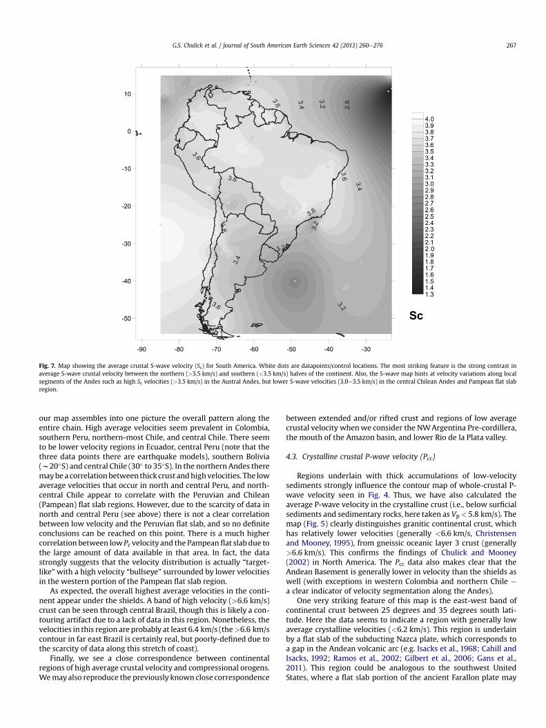
Fig. 7. Map showing the average crustal S-wave velocity (Sc) for South America. White dots are datapoints/control locations. The most striking feature is the strong contrast inaverage S-wave crustal velocity between the northern (>3.5 km/s) and southern (<3.5 km/s) halves of the continent. Also, the S-wave map hints at velocity variations along localsegments of the Andes such as high Sc velocities (>3.5 km/s) in the Austral Andes, but lower S-wave velocities (3.0e3.5 km/s) in the central Chilean Andes and Pampean flat slabregion.
G.S. Chulick et al. / Journal of South American Earth Sciences 42 (2013) 260e276 267
our map assembles into one picture the overall pattern along theentire chain. High average velocities seem prevalent in Colombia,southern Peru, northern-most Chile, and central Chile. There seemto be lower velocity regions in Ecuador, central Peru (note that thethree data points there are earthquake models), southern Bolivia(w20�S) and central Chile (30� to 35�S). In the northern Andes theremaybeacorrelationbetween thickcrust andhighvelocities. The lowaverage velocities that occur in north and central Peru, and north-central Chile appear to correlate with the Peruvian and Chilean(Pampean) flat slab regions. However, due to the scarcity of data innorth and central Peru (see above) there is not a clear correlationbetween low velocity and the Peruvian flat slab, and so no definiteconclusions can be reached on this point. There is a much highercorrelation between low Pc velocity and the Pampeanflat slab due tothe large amount of data available in that area. In fact, the datastrongly suggests that the velocity distribution is actually “target-like”with a high velocity “bullseye” surrounded by lower velocitiesin the western portion of the Pampean flat slab region.
As expected, the overall highest average velocities in the conti-nent appear under the shields. A band of high velocity (>6.6 km/s)crust can be seen through central Brazil, though this is likely a con-touring artifact due to a lack of data in this region. Nonetheless, thevelocities in this region are probably at least 6.4 km/s (the>6.6 km/scontour in far east Brazil is certainly real, but poorly-defined due tothe scarcity of data along this stretch of coast).
Finally, we see a close correspondence between continentalregions of high average crustal velocity and compressional orogens.Wemayalso reproduce the previously known close correspondence
between extended and/or rifted crust and regions of low averagecrustal velocity whenwe consider the NWArgentina Pre-cordillera,the mouth of the Amazon basin, and lower Rio de la Plata valley.
4.3. Crystalline crustal P-wave velocity (Pcc)
Regions underlain with thick accumulations of low-velocitysediments strongly influence the contour map of whole-crustal P-wave velocity seen in Fig. 4. Thus, we have also calculated theaverage P-wave velocity in the crystalline crust (i.e., below surficialsediments and sedimentary rocks, here taken as Vp< 5.8 km/s). Themap (Fig. 5) clearly distinguishes granitic continental crust, whichhas relatively lower velocities (generally <6.6 km/s, Christensenand Mooney, 1995), from gneissic oceanic layer 3 crust (generally>6.6 km/s). This confirms the findings of Chulick and Mooney(2002) in North America. The Pcc data also makes clear that theAndean Basement is generally lower in velocity than the shields aswell (with exceptions in western Colombia and northern Chile e
a clear indicator of velocity segmentation along the Andes).One very striking feature of this map is the east-west band of
continental crust between 25 degrees and 35 degrees south lati-tude. Here the data seems to indicate a region with generally lowaverage crystalline velocities (<6.2 km/s). This region is underlainby a flat slab of the subducting Nazca plate, which corresponds toa gap in the Andean volcanic arc (e.g. Isacks et al., 1968; Cahill andIsacks, 1992; Ramos et al., 2002; Gilbert et al., 2006; Gans et al.,2011). This region could be analogous to the southwest UnitedStates, where a flat slab portion of the ancient Farallon plate may
Fig. 8. Average S-wave velocity (Scc) for the crystalline crust of South America. White dots are datapoints/control locations. The most striking feature unveiled here is the lowvelocity (<3.5 km/s) zone likely corresponding to the Pampean flat slab region under Northern Chile and Argentina also stands out. The results for Scc under the Andes are againconsistent with our previous observations about “velocity bands” or velocity variations along different segments of the range.
G.S. Chulick et al. / Journal of South American Earth Sciences 42 (2013) 260e276268
underlay the region (e.g. Helmstaedt et al., 2004; Gorbatov andFukao, 2005). Just like in the southwest United States, there isa “Basin and Range” province located above this flat slab region ofSouth America; the North American Basin and Range is similarlyunderlain by very low velocity (<6.2 km/s), high heat flow crys-talline crust (Beck et al., 2005). Once again, because of a scarcity ofdata, no such conclusion can be reached about the more northerlyPeruvian “flat slab.” At best, there is just a hint of possible low Pccvelocities in this region.
Finally, note in general that Pcc velocities are lower in southernSouth America than in the northern shield regions. This is not duemerely to especially low velocity, but also several other nearbyregions with low Pcc, including northernmost Chile and the conti-nental shelf of Uruguay.
Another feature that appears on this map in the eastern PacificOcean is the Nazca Ridge, which appears here as a region withanomalously low velocity (<6.6 km/s) layer 3 oceanic crust.
The global average P-wave velocity was found to be 6.45 km/s(Christensen and Mooney, 1995), and we find good agreement forthe continent of South America (6.47 km/s). Since the averagecrystalline crustal velocity is related to the composition of the crust,the apparent global conformity of this parameter strongly supportsthe hypothesis that crustal formation has been a uniform processon a global scale for at least the past 3.0 billion years (Ga).
4.4. Sub-moho P-wave velocity (Pn)
The contour map of Pn, the seismic velocity of the uppermostlithospheric mantle, is presented in Fig. 6. It is important to observethat there is insufficient azimuthal coverage to make corrections
for seismic anisotropy. This is undoubtedly one reason why thismap shows many small-scale features. The continental-scale vari-ation in Pn velocity is anyway more likely attributable to variationin lithospheric temperature (e.g., Artemieva and Mooney, 2001),than to anisotropy. Nonetheless, several features are discernable inthis map.
Much of the continental interior is underlain bymantlewith a Pnvelocity of at least 8.0 km/s. The one notable exception to thispattern is the Andes Mountains. The Andes tend to be underlain byslightly slower uppermantle velocities (Pn< 8.0 km/s) than the restof the continental interior. This anomaly is likely related to Andeansubduction processes, as this phenomenon has been observedelsewhere at subduction zones (e.g., Iwasaki et al., 1994; Hyndmanet al., 2005) and could be indicative of serpentinization of themantle (Barklage et al., 2006). A minor disruption to this patternunder the Andes mountains occurs at about 30 degrees southlatitude where velocities are >8.0 km/s, but this may be related tothe Pampean flat slab discussed elsewhere in this paper. Thus, thispattern of behavior may reflect such features as low-velocityabove-slab mantle channels and slab geometry.
Pn along the Chilean coast and western edge of the Andes isgenerally quite low, with exceptional higher velocity segments atabout 22� S and 30� S. This may be a feature associated withdifferences in subduction along the Chilean Coast versus CentralPeru. There is a hint that the Ecuadorian/Colombian Coast may besimilar to Chile. We also note that data in southern Brazil suggeststhat Pn is also relatively low along the SE coast of Brazil.
Continental-scale variations in Pn velocity largely correlate withthe thermal state of the lithosphere, with lower Pn velocitiesassociated with higher lithospheric temperatures (e.g., Mooney and
Fig. 9. Map showing the average Sub-Moho S-wave velocity (Sn) of South America. Only 90 datapoints (white dots) were available to construct this map so it should be consideredas preliminary. Cursory examination of the Sn map indicates high velocities under the shields (old, cold craton), and low velocities under the Andes (warm, low-velocity above-slabmantle channels) as would be expected.
G.S. Chulick et al. / Journal of South American Earth Sciences 42 (2013) 260e276 269
Braile, 1989), as under portions of the Andes or by the presence ofwater. For example, the higher Pn under the north central ChileanAndes could imply lower temperatures associated with the lack ofvolcanism attributed to the “flat slab”. We observe that high Pnvalues (>8.0 km/s) are found in the Brazilian Shield and undermuch of the seafloor, while very low Pn values (<7.8 km/s) arefound beneath the region of the Argentine Basin and possibly underthe Chile Rise as it subducts.
4.5. Average crustal S-wave velocity (Sc)
There are substantially fewer available values of average whole-crustal S-wave velocity (Sc) than of Pc. Given the sparse quantity ofdata (142 values), contour maps of Sc should be interpreted withcaution.
The location of data points and contours of Sc for South Americaare shown in Fig. 7. The most striking feature is the strong contrastin average S-wave crustal velocity between the northern (>3.5 km/s) and southern (<3.5 km/s) halves of the continent. A similarvelocity dichotomy also appears in the average crustal P-wave map(Fig. 4), but is somewhat obscured by the greater local detail on thatmap due to the higher density of P-wave data available.
Furthermore, the S-wave map suggests possible velocity varia-tions along local segments of the Andes, similar to those revealed inthe P-wave maps. For example, high Sc (>3.5 km/s) appears prob-able in the Austral Andes. In contrast, lower S-wave velocities(<3.5 km/s) appear in the central Chilean Andes and the Pampeanflat slab region under northern Chile and Argentina, and undersouthern Bolivia. These low Sc regions generally correlate with the
low Pc regions, and so likely correspond to areas with high heatflow (discussed above) and/or extended crust (discussed below).
The lack of published S-wave crustal data for the seafloor limitsthe observations we can make. Several models exist for theArgentine Basin that strongly suggest Sc should be low in thisregion (w3 km/s or less), which is consistent with this beinga sedimentary basin. The lack of such data models for the BrazilBasin causes the gridding software (and subsequent contours) tounrealistically calculate an anomalously high velocity for thisregion. The 3.6 km/s contour follows very well much of the edge ofthe continent along the Atlantic Coast (and seems to be associatedwith the western edge of the Brazilian Craton).
4.6. Crystalline crustal S-wave velocity (Scc)
The average crustal S-wave velocity in the crystalline crust (Scc,see Fig. 8) was calculated in a manner analogous to that for the Pccvelocity. Here, we assume that a minimum value of 3.35 km/s (Vp/Vs¼ 1.73) defines the top of the crystalline crust.
There are several striking features revealed by this map. First,the western Amazon Basin region exhibits relatively high Scc values(>3.8 km/s), whereas much of the shield regions display somewhatlower velocity (3.6e3.7 km/s) crust. A closer look at the Brazilianshield reveals localized variations in Scc, with a general increasefrom w3.6 km/s in the interior to w4 km/s near the coast.
Perhaps the most remarkable feature shown here is the lowvelocity (<3.5 km/s) zone that corresponds to the flat slab regionunder Northern Chile and Argentina. Low Scc values are consistentwith the discussion above concerning low Pcc, in the Basin and
G.S. Chulick et al. / Journal of South American Earth Sciences 42 (2013) 260e276270
Range Province of the southwestern United States. The low velocityregion appears quite extensive and is divided in half by a NeShigher velocity “ridge” which appears to coincide with the P-wave “bullseye” of the Pampean flat slab (see above). Additionaldata in southern Bolivia has also clearly unveiled an extendedregion of very low Scc.
The results for Scc under the Andes are again consistent with ourprevious observations about “velocity bands” or velocity variationsalong segments of the Andes for P-wave models. In general Sccappears to be quite slow beneath the Andes. Higher Scc (>3.75 km/
Fig. 10. Cross sections through the South American continent. Letters represent velocity(black¼ from P-wave datapoints; red¼ from S-wave datapoints) in those locations. All datapexaggeration is w110�). (B) At latitude 20 degrees south (vertical exaggeration is w110�).degrees south (vertical exaggeration is w130�). (E) (Near the Atlantic coast, (vertical exagglayers. The red area shows the upper crust, the green area shows the middle crustal layer, anpoints using the velocity constraints described in the text.
s) occurs under the Northern and Austral Andes, while lower Scc(<3.75 km/s) occurs from central Peruwith slight evidence throughcentral Chile (in the Altiplano and the two flat slab regions, seediscussion above). An additional lateral velocity gradient fromwest(<3.7 km/s) to east (>3.8 km/s) across the southern Brazilian Shieldcan also be seen. In contrast, the relatively high Scc under much ofthe Brazilian shield, Scc is apparently still at least 0.1 km/s slowerunder the Guiana Shield. Finally, the few S-wave models availablefor oceanic crust (as in the Argentine Basin) clearly reveal oceaniclayer 3 on this map as areas of extremely high Scc (w3.9 km/s).
profiles on or near the cross section line while the numbers show the velocitiesoints lie within 300 km of the cross section line. (A) Across the Brazilian Shield (vertical(C) At latitude 33.5 degrees south (vertical exaggeration is w130�). (D) At latitude 55eration is w200�). For all maps the light blue and yellow areas show the sedimentaryd the dark blue area shows the lower crust. All layers were interpolated between data
Fig. 10. (continued).
G.S. Chulick et al. / Journal of South American Earth Sciences 42 (2013) 260e276 271
G.S. Chulick et al. / Journal of South American Earth Sciences 42 (2013) 260e276272
4.7. Sub-Moho S-wave velocity (Sn)
Only 79 data points are available to define the contour map of Snvelocity beneath South America (Fig. 9). Given the scarcity of data,this map should be considered as preliminary.
Cursory examination of the Sn map (Fig. 9) and Pn map (Fig. 6)indicates a gross similarity in distribution of high and low velocityvaluesdhigh velocities under the shields (old, cold craton), and lowvelocities under the Andes (warm, low-velocity, above-slab mantlewedge). Still, there is some hint that there are higher velocitysegments along the mountain chain e under perhaps Colombia (1point), central Chile (1 point), and the southern tip of SouthAmerica (definitely a change of regime here).
Nonetheless, there are several differences between the twocontour maps, themost notable of which is that, while there is clearevidence for high Pn in the Pampean flat slab region under theAndes, there seems to be evidence for relatively lower Sn values.Close examination of both maps and of the database velocity depthmodels shows several data points in the region that have high Pn,but relatively low Sn.
When Fig. 9 is compared to the 100-km depth S-wave velocitymap of SA99 (van der Lee et al., 2001, 2002), there are apparentgross similarities. At 100 km depth, SA99 shows fast mantleunderlying the continental interior, surrounded by slow mantleunderlying much of the continental margins. Our map of Sn showsa similar pattern, with higher Sn under the interior and lower Sncloser to the margins.
4.8. Crustal velocity structure cross-sections
Fig. 10 shows five cross sections through the South Americancontinent synthesized from nearby individual velocity depth
Fig. 11. Histogram of the raw (a) and gridded (b) crustal thickness data (Hc) of the crust in Sdata over the entire continent. Otherwise, since most of our data points are in the thicker
functions. The locations of the cross-sections are shown in thefigureinsets, and are located roughly through the Brazilian shield, at 20degrees south latitude, at 33.5 degrees south latitude, at 55 degreessouth latitude, and along the South American Atlantic coast. Verticalexaggeration varies by cross section. To construct the cross-sections,we developed contour maps in the following manner.
We selected a series of P-wave velocity horizons at 4.0, 5.8, 6.2,and 6.6 km/s, (which roughly correspond to post-Paleozoic sedi-ments, the top of the crystalline continental crust or oceanic layer2b crust, the top of the middle crust, and the top of high-velocitylower continental crust or layer 3 oceanic crust). We then appliedthese to the one-dimensional velocity-depth functions in thedatabase to determine the depths at which these horizons occur.Then, along with elevation data (provided by ETOP02, NationalGeographic Data Center, 2001) and with the Moho depth, weused the software to construct a series of contour maps of depth tothese various horizons (using a linear interpolation betweenpoints) with respect to sea level. By using the SLICE function of thesoftware and overlaying the “slices” for each contour map, wewereable to construct the desired cross-sections.
To help in the interpretation of the cross-sections, we haveoverlaid a selection of one-dimensional velocity depth functionsfrom the database that fall within a certain geographical tolerance(300 km) of each cross section line (blackdP-wave data; reddS-wave data). Many of the physical properties of the continent(such as details of the sedimentary layers, the Pampean flat slab,and the thick crustal root beneath the Andes Mountains) can beseen in the cross-sections.
The bulk of the data in the region of Pampean flat-slabsubduction is derived from the CHARGE (e.g. Wagner et al.,2005; Alvarado et al., 2009) and CHARSME (e.g. Monfret et al.,2005; Deshayes et al., 2008) experiments. The model we
outh America. The one degree gridding (shown in c) was used to average the thicknessAndean regime, our average thickness for the continent would be skewed.
G.S. Chulick et al. / Journal of South American Earth Sciences 42 (2013) 260e276 273
constructed from the contouring software reveals a bullseyepattern on the Pcc map (Fig. 5), consisting of concentric rings ofdecreasing velocity (down to <6.0 km/s) surrounding a centralregion (dome) of much higher velocity (>6.4 km/s) centered atapproximately 32�S, 68�W. This is consistent with the resultspresented in Alvarado et al. (2009). The dome coincides with theCuyana Terrane, a region Alvarado et al. (2009) identify as havingthick 60 km crust (w50 km in our model), with a relatively highlower-crustal compressional wave velocity of 6.5 km/s (repre-sented by the dome in our model). It also has a high Vp/Vs ratio of1.83 (6.4/3.5¼1.81 in our model), which sits 100 km above andapproximately 200 km to the south of the heart of the flat-slab (seeFigs. 1 and 2 of Alvarado et al., 2009).
Alvarado et al. (2009) contrast this region to the nearby PampaTerrane, which lies to the northeast, centered near 30�S, 65�W.They have identified the Pampa Terrane as a region of averagecrustal thickness (w35 km; our model gives w40 km), with a lowcompressional velocity of 6.0 km (w<6.0 km in our model) anda normal Vp/Vs ratio of 1.73 (6.0/3.5¼1.71 in our model). Theyascribe this difference to ecolgization of the lower crust of theCuyana Terrane via hydration from fluids derived from the under-lying Nazca slab.
Fig. 12. a) Histogram of the P-wave velocity of the crust (Pc) in South America. Results shvelocity of the crust (Sc) in South America. Note the slight bimodality at 3.50 and about 3.62i.e. with sediments removed. Note the slightly bimodal distribution at 6.50 and about 6.80 kResults show slight bimodality at 3.55 and near 3.70 km/s. e) Histogram of the P-wave ve8.10 km/s. f) Histogram of the S-wave velocity of the upper mantle (Sn) in South America.
4.9. Statistical analysis of the geophysical parameters
Statistical analyses of the seismic parameters appearing in thecontour maps are presented in Tables 1 and 2. The ratio of someseismic parameters (Pc/Sc, Pcc/Scc, and Pn/Sn), are also presented inTable 2. However, due to insufficient data coverage (many P-wave,1-D velocity depth models do not have corresponding S-wavemodels and vice versa), these ratios are not presented in the formof contour maps. For comparison, we present the statisticalanalyses of Christensen and Mooney (1995) for all continentsand of Chulick and Mooney (2002) for North America in Table 1.The work of Christensen and Mooney (1995) was based ona worldwide set of 560 continental seismic-refraction data points.Histograms of these seismic parameters are presented inFigs. 11 and 12.
For South America we found an average whole crustal P-wavevelocity (Pcc) of 6.47 km/s (Table 1). Since the global average Pccdetermined by Christensen and Mooney (1995) is only slightlylower (6.45 km/s), we believe that further analysis of Pcc data fromother continents should arrive at a very similar result. Indeed,Chulick and Mooney (2002) also show close agreement for NorthAmerica (6.44 km/s).
ow a slightly bimodal distribution at 6.00 and 6.20 km/s. b) Histogram of the S-wavekm/s. c) Histogram of the P-wave velocity of the crystalline crust (Pcc) in South America,m/s d) Histogram of the S-wave velocity of the crystalline crust (Scc) in South America.locity of the upper mantle (Pn) in South America. Note sharp peak between 8.00 and
G.S. Chulick et al. / Journal of South American Earth Sciences 42 (2013) 260e276274
The average value for Pn velocity under South America found bythis study (8.00 km/s) is just slightly lower than the 8.07 km/sglobal average of Christensen and Mooney (1995), and very similarto the 8.02 km/s found for North America by Chulick and Mooney(2002). Given the large statistical populations used in these anal-yses, the various continental estimates of average Pn velocityappear to be well-determined values that are unlikely to changedramatically as additional measurements are compiled. It must benoted, however, that all of these statistical analyses assume a seis-mically isotropic mantle. An estimated 6% anisotropy will providelocal azimuthally-dependent variations in Pn velocity of �0.5 km/s(i.e., 7.5e8.5 km/s). Variations inmantle composition and especiallyin temperature are also important factors in determining Pnvelocity (Artemieva and Mooney, 2001).
The histograms of the data used for the contour maps ofFigs. 3e9 provide additional insights into the properties of thecrust. The modal value of crustal thickness from the statistics andsubsequent histogram for the original unweighted data is43.83 km (Fig. 11a), a value that may be considered as thick cruston a global basis (Christensen and Mooney, 1995). As discussedabove, this high modal value is skewed due to the numerouscrustal profiles in Andean South America and the relative paucityof data from the middle of the continent. Fig. 11a shows that overhalf of all continental crustal thickness measurements exceed40 km. However, a histogram constructed from 1832 grid pointsused to find the weighted average (Fig. 11b) produces a truer“bell-shaped curve,” with a modal value of w38 km, near theweighted average value of 38.17 km. This weighted average is thevalue for Hc given in Table 2.
The histogram for Pc (Fig. 12a) shows two modest peaks. This isalso hinted at in the histogram for Sc (Fig. 12b) as well as that forPcc and Scc (Fig. 12c and d), demonstrating that the averagevelocity of the South American continental crust is bi-modal forboth P- and S-waves. Our global database shows that similar plotsof Pcc for all the other continents (with the exception ofAntarctica, where data are extremely sparse) display the same bi-modality (Chulick and Mooney, 2002). We interpret this bi-modality as indicating the probable existence of two end-member types of continental crust. What distinguishes thesetwo crustal types is the presence or absence of a high-velocity(6.9e7.3 km/s) lower crustal layer. Thin (20e35 km) crustcommonly lacks a high-velocity lower crustal layer and has a low(w<6.5 km/s) average crustal velocity as per Pcc. Thick(35e50 km) crust, particularly that of stable continental interiors(i.e., platforms and shields), often has a high-velocity lowercrustal layer and therefore, has a relatively high (w>6.5 km/s)average crustal velocity (Meissner, 1986; Mooney et al., 1998).Together, these two crustal types provide a global average ofcontinental crustal velocity of 6.45 km/s.
Pn velocity peaks sharply around the average value of 7.998 km/s(Fig. 12e). More than 75% of all of the measurements of Pn velocityfall in the range 7.8e8.2 km/s, as anticipated from anisotropyconsiderations. The Sn velocity peaks around 4.50 km/s(Fig. 12f), near the statistical average of 4.504 km/s (Table 2).
5. Conclusions
We present new contour maps and a statistical analysis of theseismic structure of the crust and uppermost mantle of SouthAmerica and the surrounding ocean basins. These results are basedon a large number of new seismic measurements, including datafrom some previously unexplored regions. We have primarily usedresults from seismic-refraction surveys, with additional dataacquired primarily from earthquake tomography studies, surface-
wave analyses, and receiver functions (Table 3). From our analysiswe conclude:
1) The weighted average of 889 measurements of continentalcrustal thickness (Hc) for South America is 38.17 km. Thisis w1 km less than the global average of 39.2 km (Christensenand Mooney, 1995) and reflects the inclusion into our analysisof both numerous marine measurements made on the shallowand thin (20e25 km) continental shelf, as well as the thickerAndean crust.
2) Histograms of whole crustal average P- and S-wave velocities ofthe crystalline crust are generally bi-modal. A lower averagecrustal velocity (w<6.5 km/s) correlates with thin crust thatlacks a high-velocity (6.9e7.3 km/s) lower crustal layer. Ahigher average crustal velocity (w>6.5 km/s) correlates withthemoderately thick (w40 km) crust of the continental interiorthat includes a high-velocity basal crustal layer.
3) The average P-wave velocity of the eastern Pacific Ocean crustis higher than that of the western Atlantic Ocean crust due toa thinner sediment layer (layer 1) in the eastern Pacific Ocean.This supports a similar observation by Chulick and Mooney(2002) for the Atlantic and Pacific Ocean basins off NorthAmerica.
4) The average P-wave velocity of the crystalline crust of SouthAmerica is found to be 6.47 km/s, which is nearly equal to theglobal average of 6.45 km/s determined by Christensen andMooney (1995). Since the average crustal velocity is related tothe composition of the crust, the uniformity of this parameterstrongly supports the hypothesis that crustal formation has beena uniform process on a global scale for at least the past 3.0 Ga.
5) The average Pn velocity under South America is 8.00 km/s, withmore than 75% of all measurements falling in the range of7.8e8.2 km/s.
6) The thickness of the crust under the Andes is relatively large,but highly variable. The Andean crust ranges from more than60 km thick beneath northern Colombia and the Altiplano,a possible Tibetan Plateau analog, to a minimum of 30 km atTierra del Fuego.
7) There is some evidence given the shallowMoho depths that thecrust is extended in the regions between the Andes and theGuiana and Brazilian Shields that typically have a crustalthickness >40 km.
8) There are strong variations in seismic velocity along the lengthof theAndes, suggesting localizedmodifications in the tectonics.
9) The region of South America above the Pampean flat slabsegment of the subducting Nazca plate appears to be a modernanalog to the tectonic regime of the southwestern United States.Apart from the previously recognized Basin and Range Provincein thePre-Cordillera, this region isunderlainbyvery lowP-andS-wavecrustal velocities, alongwith thinnedcrust.Data coverage isinsufficient to draw similar conclusions about the Peruvian flatslab region although hints of low velocity are observed.
10) Regional variations in oceanic crustal and uppermantle seismicvelocities appear to distinguish certain oceanic geographicfeatures, including the Nazca Ridge, the Chile Ridge, and theArgentine Basin.
The complete South American database and the associated list ofsource referencesmay be obtained on the Internet from the authorsat: http://earthquake.usgs.gov/research/structure/crust/sam.php.
Acknowledgements
Support for this study by the National Earthquake HazardsProgram of the USGS is gratefully acknowledged. Reviews by Mark
G.S. Chulick et al. / Journal of South American Earth Sciences 42 (2013) 260e276 275
Goldman, Christian Guillemot, Pat McCrory, Jesse Kass, LeahCampbell, and two anonymous reviewers from the journal wereextremely insightful and useful. Additional thanks are due to NeilFenning andAlex Ferguson forhelpwithdata compilation andfigureediting.
References
Agudelo, W., Ribodetti, A., Collot, J.Y., Operto, S., 2009. Joint inversion of multi-channel seismic reflection and wide-angle seismic data; improved imaging andrefined velocity model of the crustal structure of the north Ecuador-southColombia convergent margin. J. Geophys. Res. 114, B02306. http://dx.doi.org/10.1029/2008JB005690.
Alvarado, P., Beck, S., Zandt, G., Araujo, M., Triep, E., 2005. Crustal deformation in thesouth central Andes backarc terranes as viewed from regional broad-bandseismic waveform modeling. Geophys. J. Int. 163, 580e598.
Alvarado, P., Beck, S., Zandt, G., 2007. Crustal structure of the south-central AndesCordillera and backarc region from regional waveform modeling. Geophys. J.Int. 170, 858e875.
Alvarado, P., Pardo, M., Gilbert, H., Miranda, S., Anderson, M., Saez, M., Beck, S., 2009.Flat slab subduction and crustal models for the seismically active sierraspampeanas region of Argentina. Memoir e Geological Society of America 204,261e278. http://dx.doi.org/10.1130/2009.1204(12).
An, M., Assumpção, M.S., 2004. Multi-objective inversion of surface waves andreceiver functions by competent genetic algorithms applied to the crustalstructure of the Parana Basin, SE Brazil. Geophys. Res. Lett. 31, 1e4.
An, M., Assumpção, M., 2005. Effect of lateral variation and model parameterizationon surface wave dispersion inversion to estimate the average shallow structurein the Parana Basin. J. Seismol. 9, 449e462.
ANCORPWorking Group, 2003. Seismic imaging of a convergent continental marginand plateau in the Central Andes (Andean Continental Research Project 1996).J. Geophys. Res. 108, 25. http://dx.doi.org/10.1029/2002JB001771.
Artemieva, I.M., Mooney, W.D., 2001. Thermal thickness and evolution of thePrecambrian lithosphere: a global study. J. Geophys. Res. 106, 16,387e16,414.
Assumpção, M., James, D., Snoke, A., 2002. Crustal thinknesses in SE Brazilian Shieldby receiver function analysis: Implications for isostatic compensation.J. Geophys. Res. 107 (B1), 2-1e2-14. http://dx.doi.org/10.1029/2001JB000422.
Assumpção, M., An, M., Bianchi, M., França, G.S.L., Rocha, M., Barbosa, J.R.,Berrocal, J., 2004. Seismic studies of the Brasília fold belt at the western borderof the São Francisco Craton, Central Brazil, using receiver function, surface-wavedispersion and teleseismic tomography. Tectonophysics 388, 173e185.
Balling, N., 1995. Heat flow and thermal structure of the lithosphere across theBaltic Shield and northern Tornquist Zone. Tectonophysics 244, 13e50.
Barklage, M.E., Conder, J., Wiens, D., Shore, P., Shiobara, H., Sugioka, H., Zhang, H.,2006. 3-D seismic tomography of the Mariana Mantle Wedge from the2003e2004 passive component of the Mariana subduction factory imagingexperiment. EOS Trans. Am. Geophys. Union. 87, no. 52, Suppl. 26.
Bassin, C., Laske, G., Masters, G., 2000. The current limits of resolution for surfacewave tomography in South America. EOS Trans. Am. Geophys. Union 81, F897.http://igppweb.ucsd.edu/wgabi/crust2.html.
Baumont, D., Paul, A., Zandt, G., Beck, S.L., 2001. Inversion of Pn travel times forlateral variations of Moho geometry beneath the Central Andes and comparisonwith the receiver functions. Geophys. Res. Lett. 28, 1663e1666.
Baumont, D., Paul, A., Zandt, G., Beck, S.L., Pedersen, B., 2002. Lithospheric structureof the Central Andes based on surface wave dispersion. J. Geophys. Res. 107,2371. http://dx.doi.org/10.1029/2001JB000345.
Beck, S., Zandt, G., Myers, S., Wallace, T., Silver, P., Drake, L., 1996. Crustal-thicknessvariations in the Central Andes. Geology 24, 407e410.
Beck, S.L., Zandt, G., 2002. The nature of orogenic crust in the Central Andes.J. Geophys. Res. 107, 2230. http://dx.doi.org/10.1029/2000JB000124.
Beck, S., Gilbert, H., Wagner, L., Alvarado, P., Zandt, G., 2005. The Sierras Pampeanasof Argentina: a modern analog for the Laramide Rocky Mountains in thewestern U.S. Earthscope meeting, New Mexico.
Berrocal, J., Marangoni, Y., De Sa, N.C., Fuck, R., Soares, J.E.P., Dantas, E., Perosi, F.,Fernandes, C., 2004. Deep seismic refraction and gravity crustal model andtectonic deformation in Tocantins Province, Central Brazil. Tectonophysics 388,187e199.
Bezada, M.J., Schmitz, M., Jacome, M.I., Rodriguez, J., Audemard, F., Izarra, C.,Broadband Ocean-Land Investigations of Venezuela and the Antilles Arc Region(BOLIVAR) Active Seismic Working Group, (III), 2008. Crustal structure in theFalcon Basin area, northwestern Venezuela, from seismic and gravimetricevidence. J. Geodyn. 45, 191e200.
Blaich, O.A., Tsikalas, F., Faleide, J.I., 2008. Northeastern Brazilian margin; regionaltectonic evolution based on integrated analysis of seismic reflection andpotential field data and modelling; geodynamics of lithospheric extension.Tectonophysics 458, 51e67.
Blaich, O.A., Faleide, J.I., Tsikalas, F., Franke, D., Leon, E., 2009. Crustal-scale archi-tecture and segmentation of the Argentine margin and its conjugate off SouthAfrica. Geophys. J. Int. 178, 85e105.
Blaich, O.A., Faleide, J.I., Tsikalas, F., 2011. Crustal Breakup and ContinenteOceanTransition at South Atlantic Conjugate Margins. J. Geophys. Res. 116 (B01402).http://dx.doi.org/10.1029/2010JB007686
Blundell, D., Freeman, R., Mueller, S. (Eds.), 1992. A Continent RevealeddTheEuropean Geotranverse. Cambridge Univ. Press, p. 275.
Bohm, M., Luth, S., Echtler, H., Asch, G., Bataille, K., Bruhn, C., Rietbrock, A.,Wigger, P., 2002. The Southern Andes between 36� and 40� S latitude: seis-micity and average seismic velocities. Tectonophysics 356, 275e289.
Bostock, M.G., 1999. Seismic imaging of lithospheric discontinuities and continentalevolution. Lithos 48, 1e16.
Cahill, T., Isacks, B.L., 1992. Seismicity and the shape of the subducted Nazca plate.J. Geophys. Res. 97, 17503e17529.
Christensen, N.I., Mooney, W.D., 1995. Seismic velocity structure and composition ofthe continental crust: a global view. J. Geophys. Res. 100 (B7), 9761e9788.
Christeson, G.L., Mann, P., Escalona, A., Aitken, T.J., 2008. Crustal structure of theCaribbean-northeastern South America arc-continent collision zone. J. Geophys.Res. 113, B08104. http://dx.doi.org/10.1029/2007JB005373.
Chulick, G.S., 1997. Comprehensive seismic survey database for developing three-dimensional models of the Earth’s crust, Seismo. Res. Lett. 68 (5), 734e742.
Chulick, G.S., Mooney, W.D., 2002. Seismic structure of the crust and Uppermostmantle of North America and Adjacent Ocean basins: a synthesis. Bull. Seis. Soc.Am. 92 (6), 2478e2492.
Collins, C.D.N., 1988. Seismic velocities in the crust and upper mantle of Australia,Bureau of Mineral Resources, Geol. Geophys. Rept. 277, Aust. Gov’t. Publ.Service, Canberra, Australia, 159 pp.
Cordani, U.G., Teixeira, W., D’Agrella-Filho, M.S., Trindade, R.I., 2009. The position ofthe Amazonia craton in supercontinents. Gondwana Res. 15, 396e407.
Cordani, U.G., Teixeira, W., Tassinari, C.C.G., Coutinho, J.M.V., Ruiz, A.S., 2010. The RioApa Craton in Mato Grosso du Sol (Brazil) and Northern Paraguay: Geochro-nological Evolution, correlations and tectonic implications for Rodinia andGondwana. Am. J. Sci. 310, 981e1023. http://dx.doi.org/10.2475/09.2010.09.
Deshayes, P., Monfret, T., Pardo, M., Vera, E., 2008. Three-dimensional P- and S-waveseismic attenuation models in central Chile e western Argentina (30� e 34� S)from local recorded earthquakes. In: 7th International Symposium on AndeanGeodynamics (ISAG, 2008 Nice, France) Extended Abstracts, pp. 184e187.
Dorbath, C., 1996. Velocity structure of the Andes of central Peru from locallyrecorded earthquakes. Geophys. Res. Lett. 23, 205e208.
Eaton, D., Mereu, R., Jones, A., Hyndman, R., 2005. The Moho beneath the CanadianShield. Geophys. Res. Abst. 7, 05568.
Feng, M., Assumpção, M., van der Lee, S., 2004. Group-velocity tomography andlithospheric S-velocity structure of the South American continent. Phys. EarthPlan. Int. 147, 315e331.
Feng, M., van der Lee, S., Assumpção, M., 2007. Upper mantle structure of SouthAmerica from joint inversion of waveforms and fundamental mode groupvelocities of Rayleigh waves. J. Geophys. Res. 112, B04312. http://dx.doi.org/10.1029/2006JB004449.
Flueh, E.R., Vidal, N., Ranero, C.R., Hojka, A., Von Huene, R., Bialas, J., Hinz, K.,Cordoba, D., Danobeitia, J.J., Zelt, C., 1998. Seismic investigation of the conti-nental margin off- and onshore Valparaiso, Chile. Tectonophysics 288, 251e263.
Fromm, R., Zandt, G., Beck, S.L., 2004. Crustal thickness beneath the Andes andSierras Pampeanas at 30�S inferred from Pn apparent phase Velocities. Geo-phys. Res. Lett. 31, L06625. http://dx.doi.org/10.1029/2003GL019231.
Fuck, R., Bley Briton Eves, B., Schobbenhaus, C., 2008. Rodinia descendents in SouthAmerica. Precambrian Res. 160, 108e126.
Gans, C.R., Beck, S.L., Zandt,G., Gilbert,H., Alvarado,P., Anderson,M., Linkimer, L., 2011.Continental and Oceanic Crustal Structure of the Pampean flat slab region,western Argentina, using receiver function analysis: newhigh-resolution results.Geophys. J. Int. 186, 45e58. http://dx.doi.org/10.1111/j.1365-246X.2011.05023.x.
Gilbert, H., Beck, S., Zandt, G., 2006. Lithospheric and upper mantle structure ofcentral Chile and Argentina. Geophys. J. Int. 165, 383e398. http://dx.doi.org/10.1111/j.1365-246X.2006.02867.
Golden Software, 2009. Surfer 9. http://www.goldensoftware.com/products/surfer/.Gorbatov, A., Fukao, Y., 2005. Tomographic search for missing link between the
ancient Farallon subduction and the present Cocos subduction. Geophys. J. Int.160, 849e854.
Greenroyd, C.J., Peirce, C., Rodger, M., Watts, A.B., Hobbs, R.W., 2007. Crustalstructure of the French Guiana margin, West Equatorial Atlantic. Geophys. J. Int.169, 964e987.
Heit, B., Yuan, X., Bianchi, M., Sodoudi, F., Kind, R., 2008. Crustal thickness esti-mation beneath the southern Central Andes at 30 S and 36 S from S waveReceiver Function Analysis. Geophys. J. Int. 174, 249e254.
Helmstaedt, H., Usui, T., Nakamura, E., Maruyama, S., 2004. Syn-Laramide UHPmetamorphism under the Colorado Plateau; xenolith evidence for Proterozoicaccretionary tectonics or flat subduction of the Farallon Plate? Abst. Progr. Geol.Soc. Am. 36, 210.
Hyndman, R.D., Currie, C.A., Mazotti, S., 2005. Subduction zone backarcs, mobilebelts, and orogenic heat. GSA Today 15, 4e10.
Isacks, B., Oliver, J., Sykes, L., 1968. Seismology and the new Global Tectonics.J. Geophys. Res. 73, 5855e5899.
Iwasaki, T., Yoshii, T., Moriya, T., Kobayashi, A., Nishiwaki, M., Tsutsui, T., Iidaka, T.,Ikami, A., Matsuda, T., 1994. Precise P and S wave velocity structures in theKitakami massif, northern Honshu, Japan, from a seismic refraction experiment.J. Geophys. Res. 99, 22187e22204.
James, D.E., 1971. Plate tectonic model for the evolution of the Central Andes. Geol.Soc. Am. Bull. 82, 3325e3346.
James, D.E., Snoke, J.A., 1994. Structure and tectonics in the region of flat subductionbeneath central Peru; crust and uppermost mantle. J. Geophys. Res. 99,6899e6912.
G.S. Chulick et al. / Journal of South American Earth Sciences 42 (2013) 260e276276
Julia, J., Assumpção, M., Rocha, M.P., 2008. Deep crustal structure of the ParanaBasin from receiver functions and Rayleigh-wave dispersion; evidence fora fragmented cratonic root. J. Geophys. Res. 113, B08318. http://dx.doi.org/10.1029/2007JB005374.
Lange, D., Rietbrock, A., Haberland, C., Bataille, K., Dahm, T., Tilmann, F., Flueh, E.R.,2007. Seismicity and geometry of the south Chilean subduction zone(41.5�Se43.5�S): Implications for controlling parameters. Geophys. Res. Lett. 34,1e5.
Lawrence, J.F., Wiens, D.A., 2004. Combined receiver-function and surface wavephase-velocity inversion using a Niching Genetic Algorithm: application toPatagonia. Bull. Seis. Soc. Am. 94, 977e987.
Lloyd, S., van der Lee, S., França, G.S., Assumpção, M., Feng, M., 2010. Moho map ofSouth America from Receiver Functions and Surface Waves. J. Geophys. Res. 115,B11315. http://dx.doi.org/10.1029/2009JB006829.
Meissner, R., 1986. The Continental Crust: A Geophysical Approach. Academic Press,London, 426 pp.
Monfret, T., Pardo, M., Salazar, P., Vera, E., Eisenberg, A., Yañez, G., 2005. Threedimensional P and S wave velocity models in central Chile and westernArgentina (31�e34�S) from local data: no tear between the flat and steepsegments of the Nazca plate. In: 6th International Symposium on AndeanGeodynamics (ISAG 2005, Barcelona), Extended Abstracts, pp. 516e519.
Mooney, W.D., Meyer, R.P., Laurence, J.P., Meyer, H., Ramirez, J.E., 1979. Seismicrefraction studies of the western cordillera Colombia. Bull. Seis. Soc. Am. 69,1745e1761.
Mooney, W.D., 1989. Seismic methods for determining earthquake source param-eters and lithospheric structure. In: Pakiser, L.C., Mooney, W.D. (Eds.),Geophysical Framework of the Continental United States. Geol. Soc. Am.Memoir, vol. 172, pp. 11e34.
Mooney, W.D., Braile, L.W., 1989. The seismic structure of the continental crust andupper mantle of North America. In: Bally, A.W., Palmer, A.R. (Eds.), The Geologyof North AmericadAn Overview. Geological Society of America, Boulder, CO,pp. 39e52.
Mooney, W.D., Laske, G., Masters, T.G., 1998. CRUST 5.1: a global crustal model at 5�
x 5� . J. Geophys. Res. 103, 727e747.Myers, S.C., Beck, S., Zandt, G., Wallace, T., 1998. Lithospheric-scale structure across
the Bolivian Andes from tomographic images of velocity and attenuation for Pand S waves. J. Geophys. Res. 103, 21233e21252.
Nataf, H.-C., Richard, Y., 1996. 3SMAC: an a priori tomographic model of theupper mantle based on geophysical modeling. Phys. Earth Planet. Int. 95,101e122.
National Geographic Data Center, 2001. ETOP02. http://ols.nndc.noaa.gov/plolstore/plsql/olstore.prodspecific?prodnum¼G02092-DVD-A0001 (accessed 05.02.12).
Pakiser, L.C., Mooney, W.D., 1989. Introduction. In: Pakiser, L.C., Mooney, W.D. (Eds.),Geophysical Framework of the Continental United States. Memoir e GeologicalSociety of America, vol. 172, pp. 1e9.
Patzwahl, R., Mechie, J., Schulze, A., Giese, P.,1999. Two-dimensional velocitymodels ofthe Nazca plate subduction zone between 19.5 S and 25 S fromwide-angle seismicmeasurements during the CINCA95 project. J. Geophys. Res. 104, 7293e7317.
Pavlenkova, N.I., 1996. Crust and upper mantle structure in northern Eurasia fromseismic data. Adv. Geophys. 37, 1e133.
Pavlenkova, N.I., Pilipenko, V.N., Verpakhovskaja, A.O., Pavlenkova, G.A.,Filonenko, V.P., 2009. Crustal structure in Chile and Okhotsk Sea regions; deepseismic profiling of the continents and their margins. Tectonophysics 472,28e38.
Prodehl, C., 1984. Structure of the earth’s crust and upper mantle. In: Fuchs, K.,Soffel, H., Hellwege, K.-H. (Eds.), Landolt Bornstein New Series e PhysicalProperties of the Interior of the Earth, the Moon and the Planets. Numericaldata and functional relationships in science and technology. Group V, vol. 2a.Springer, Berlin-Heidelberg, pp. 97e206.
Ramos, V., Cristallini, E., Perez, D.J., 2002. The Pampean flat-slab of the CentralAndes. J. South Am. Earth Sci. 15, 59e78.
Regnier, M., Chiu, J.M., Smalley, R., Isacks, B.L., Araujo, M., 1994. Crustal thicknessvariation in the Andean Foreland, Argentina, from Converted Waves. Bull. Seis.Soc. Am. 84, 1097e1111.
Rodger, M., Watts, A.B., Greenroyd, C.J., Peirce, C., Hobbs, R.W., 2006. Evidence forunusually thin oceanic crust and strong mantle beneath the Amazon fan.Geology 34, 1081e1084.
Scherwath, M., Flueh, E., Grevemeyer, I., Tilmann, F., Contreras-Reyes, E.,Weinrebe, W., 2006. Investigating subduction zone processes in Chile. EOS 87,265e269.
Schmitz, M., 1994. A balanced model of the southern Central Andes. Tectonics 13,484e492.
Schmitz, M., Lessel, K., Giese, P., Wigger, P., Araneda, M., Bribach, J., Graeber, F.,Grunewald, S., Haberland, C., Lueth, S., Roewer, P., Ryberg, T., Schulze, A., 1999.The crustal structure beneath the Central Andean forearc and magmatic arc asderived from seismic studies; the PISCO 94 experiment in northern Chile (21degreese23 degrees S). J. South Am. Earth Sci. 12, 237e260.
Schmitz, M., Chalbaud, D., Castillo, J., Izarra, C., 2002. The crustal structure of theGuayana Shield, Venezuela, from seismic refraction and gravity data. Tectono-physics 345, 103e118.
Schmitz, M., Martins, A., Izarra, C., Jácome, M.I., Sánchez, J., Rocabado, V., 2005. Themajor features of the crustal structure in north-eastern Venezuela from deepwide-angle seismic observations and gravity modeling. Tectonophysics 399,109e124.
Schnabel, M., 2007. A deep seismic model for the Argentine continental margin.BGR. http://www.bgr.bund.de/cln_145/nn_336750/EN/Themen/MeerPolar/Meeresforschung/Projekte__und__Beitraege/Sued__Atlantik/seismic__model__argentina__en.html (accessed 12.22.09).
Soares, J.E., Berrocal, J., Fuck, R.A., Mooney, W.D., Ventura, D.B.R., 2006. Seismiccharacteristics of central Brazil crust and upper mantle: a deep seismicrefraction study. J. Geophys. Res. 111, B12302,. http://dx.doi.org/10.1029/2005JB003769.
Tavera, H., Fernandez, E., Bernal, I., Antayhua, Y., Agueero, C., Rodriguez, H.S.S.,Vilcapoma, L., Zamudio, Y., Portugal, D., Inza, A., Carpio, J., Callo, F., Valdivia, I.,2006. The southern region of Peru earthquake of June 23rd, 2001. J. Seismol. 10,171e195.
van der Lee, S., James, D., Silver, P., 2001. Upper mantle S velocity structure of centraland western South America. J. Geophys. Res. 106 (B12), 30821e30834.
van der Lee, S., James, D., Silver, P., 2002. Correction to “Upper mantle S velocitystructure of central and western South America”. J. Geophys. Res. 107 (B5).http://dx.doi.org/10.1029/2001JB001891
Wagner, L.S., Beck, S., Zandt, G., 2005. Upper mantle structure in the south centralChilean subduction zone (30� to 36�S). J. Geophys. Res. 110, B01308. http://dx.doi.org/10.1029/2004JB003238, pp. 1e20.
Wigger, P.J., Schmitz, M., Araneda, M., Asch, G., Baldzuhn, S., Giese, P., Heinsohn, W.-D., Martinez, E., Ricaldi, E., Roewer, P., Viramonte, J., 1994. Variation in thecrustal structure of the southern central Andes deduced from seismic refractioninvestigations. In: Reutter, K.-J., Scheuber, E., Wigger, P.J. (Eds.), Tectonics of theSouthern Central Andes (Structure and Evolution of an Active ContinentalMargin). Springer Verlag, p. 333.
Wölbern, I., Heit, B., Yuan, X., Asch, G., Kind, R., Viramonte, J., Tawackoli, S., Wilke, H.,2009. Receiver Function Images from the Moho and the slab beneath the Alti-plano and Puna plateaus in the Central Andes. Geophys. J. Int. 177, 296e308.
Yoon, M., Buske, S., Shapiro, S.A., Wigger, P., 2009. Reflection image spectroscopyacross the Andean subduction zone. Tectonophysics 472, 51e61.
Yuan, X.-C., 1996. Atlas of Geophysics in China. Geological Publishing House, Beijing,China, 217 pp.
Yuan, X., Sobolev, S.V., Kind, R., Oncken, O., Bock, G., Asch, G., Schurr, B., Graeber, F.,Rudloff, A., Hanka, W., Wylegalla, K., Tibi, R., Haberland, C., Rietbrock, A.,Giese, P., Wigger, P., Rower, P., Zandt, G., Beck, S., Wallace, T., Pardo, M.,Comte, D., 2000. Subduction and collision processes in the Central Andesconstrained by converted seismic phases. Nature 408, 958e961.
Yuan, X., Sobolev, S.V., Kind, R., 2002. Moho topography in the Central Andes and itsgeodynamic implications. Earth Planet. Sci. Lett. 199, 389e402.