7618 October, 1970 HY 10 .,'

Journal of the

HYDRAULICS DIVISION

Proceedings of the American Society of Civil Engineers

PREDICTING CONCENTRATION PROFILES IN OPEN CHANNE LSa

By Harvey E. Jobson,' A. M. ASCE and William W. S a ~ r e , ~ M. ASCE

INTRODUCTION

The exact nature of transport and mixing processes in turbulent flow has long intrigued fluid dynamicists and engineers. Problems in waste dispersion . have stimulated interest in the turbulent diffusion and convective dispersion processes. Yet it is clear that much remains to be learned before these pro- cesses are completely understood. In July, 1967 the U.S. Geological Survey, Department of the Interior, launched a project to experimentally determine I

' I the vertical component of the local mass transfer coefficient for fluid and particulate dispersants in an open channel flow. As part of this project a com- Il puter program was written to numerically solve the equation of mass con- servation for a two-dimensional steady flow. This program computes the

I

spatial distribution of a dispersant which is injected continuously into a I

steady, two-dimensional open channel flow. The program was initially used a s an aid in planning the laboratory ex-

periments. However, the solutions obtained proved to be very instructive in themselves. This paper presents some of the solutions in order to illustrate the effects of various hydraulic parameters on the predicted concentrations. It is believed these solutions provide some insight into the mechanics of diffusion.

After presenting the governing differential equation, the numerical solu- tion will be briefly analyzed. The solution i s verified for accuracy by com- parison with an analytic solution obtained for a ,special case. The ability of the governing differential equation to describe the physical process is then illustrated by comparingthe solution with laboratory data. Next the governing

;Note.-Discussion open until March 1, 1971. To extend the closing date one month, a written request must be filed with the Executive Director, ASCE. This paper is part of the copyrighted Journal of the Hydraulics Division, Proceedings of the American Society of Civil Engineers, Vol. 96, No. HY10, October, 1970. Manuscript was sub- mitted for review for possible publication on March 13, 1970.

aPresented at the Jan. 26-30, 1970, ASCE National Water Resources Engineering Meeting, held at Memphis, Tenn.

Research Hydr. Engr., U.S. Geological Survey, Fort Collins, Colo. =Research Engr., Inst. of Hydr. Research, and Assoc. Prof., Dept. of Mechanics

and Hydraulics, The Univ. of Iowa, Iowa City, Iowa.

1984 October, 1970 HY 10

equation is solved for different hydraulic conditions and the results a re shown in graphical form. The solutions indicate the fall velocity controls the rate of descent of the dispersant mass but has little effect on the rate of dispersant spread. Likewise, the transfer coefficient controls the rate of dispersant spread but has little effect on its rate of descent. The solutions also illustrate the dispersant distributions are not very sensitive to the assumed distribution of the transfer coefficient.

The data contained herein are identical to those in a dissertation by Jobson (6).

DEVE LOPMENT OF PFtEDICTION EQUATION

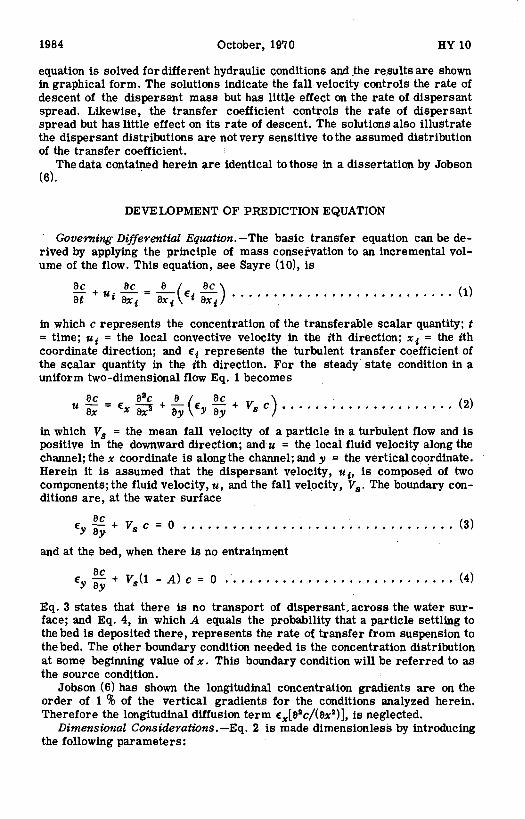
Governing Differential Equation.-The basic transfer equation can be de- rived by applying the principle of mass conservation to an incremental vol- ume of the flow. This equation, see Sayre (101, is

in which c represents the concentration of the transferable scalar quantity; t = time; u t =. the local convective velocity in the ith direction; x i = the ith coordinate direction; and ct represents the turbulent transfer coefficient of the scalar quantity in the zYh direction. For the steady state condition in a uniform two-dimensional flow Eq. 1 becomes

in which V, = the mean fall velocity of a particle in a turbulent flow and is positive in the downward direction; and u = the local fluid velocity along the channel; the x coordinate is along the channel; and y = the vertical coordinate. Herein it is assumed that the dispersant velocity, ui, is composed of two components; the fluid velocity, u, and the fall velocity, V,. The boundary con- ditions are, a t the water surface

and a t the bed, when there is no entrainment

Eq. 3 states that there is no transport of dispersant,across the water sur- face; and Eq. 4, in which A equals the prpbability that a particle settling to the bed is deposited there, represents the rate of transfer from suspension to the bed. The other boundary condition needed is the concentration distribution a t some beginning value of x . This boundary condition will be referred to a s the source condition.

Jobson (6) has shown the longitudinal concentration gradients are on the order of 1 96 of the vertical gradients for the conditions analyzed herein. Therefore the longitudinal diffusion term E , [ ~ ~ c / ( ~ x ~ ) ] , i s neglected.

Dimensional Considerations.-Eq. 2 is made dimensionless by introducing the following parameters:

HY 10 PREDICTING CONCENTRATION PROFILES

= q Relative depth YN

= % Dimensionless f a l l velocity K U , 6

E = , - Dimensionless velocity U

E 4 = ' V = J) Dimensionless transfer coefficient - K YNu+ Em - '3 = ' U* = X Dimensionless distance from source U Y & 6 U Y N

in which YN = the depth of flow, K = the Von Karman turbulence coefficient; u, = the shear velocity; em = the momentum transfer coefficient; and the bars indicate a depth averaged value. Term V S / ~ u , is often referred to a s the Rouse number. The depth averaged value of the momentum transfer coefficient in K YN 2(*/6 for a flow wherein the velocity distribution is loga- rithmic and the shear stress distribution is linear. Thus the depth averaged value of J, is the inverse of the turbulent Schmidt number. The longitudinal distance, x , is scaled by the product of the mean velocity and an index of the time required for complete mixing in the vertical. This index, sometimes known a s the Eulerian time scale for dispersion, has proven useful in dis- persion, studies (4,101. Using these scaling parameters and neglectingthe longitudinal diffusion term, Eq. 2 can be written

Numerical Solution. -Eq. 6 was numerically solved by the explicit four point forward difference scheme (9). For this scheme the flow domain is divided into N rows in the vertical and M columns iq the longitudinal direction per unit of length, i.e. the flow domain is divided into N X M differential areas per unit length of channel. The concentration and fluid velocity were assumed constant in each differential area. Subscripts i and j identify the row and col- umn of the differential area, respectively. The rows are numbered from the floor to the surface and the column numbers increase in the downstream di- rection. Term U Z ( ~ ) i s evaluated at the center of the differential area and ~ ( i ) is evaluated one-half a step lower, i.e.,at the bottom of the differential area. Term VS = v,.

With this scheme the general finite difference form of Eq. 6 becomes

in which DY = 1/N and DX = 1/M. Eq. 7 can be solvedexplicitly for&, j + 1). In order to obtain solutions for the differential areas along the boundaries,

Eqs. 3,and 4, in finite difference form, must be substituted into Eq. 7. Verification of Finite Difference Solution. -Dobbins (3) obtained analytical

1986 October, 1970 HY 10

solutions to Eq. 6 for the simplified conditions that both the velocity andthe transfer coefficient a r e constant and the probability of deposit is 1.0. To check the accuracy of the finite difference program, i ts solution was com- pared with the analytical solution given by Dobbins.

The solutions were f i r s t compared for the special case where the fall ve- locity i s zero. For this case, it was assumed that J , = p = 1.0. The assump- tion that J , = 1 is equivalent to assuming the turbulent Schmidt number is unity and, of course, p is unity for a uniform velocity distribution. At X = 0 the source condition was c = 0 for 0 5 q < 0.96 and c = 25.0 for 0.96 5 q 5

1.0. The predicted concentrations obtained from the numerical and analytical solutions differed at most by 0.1 O/o when DY for the numerical solution was 0.02.

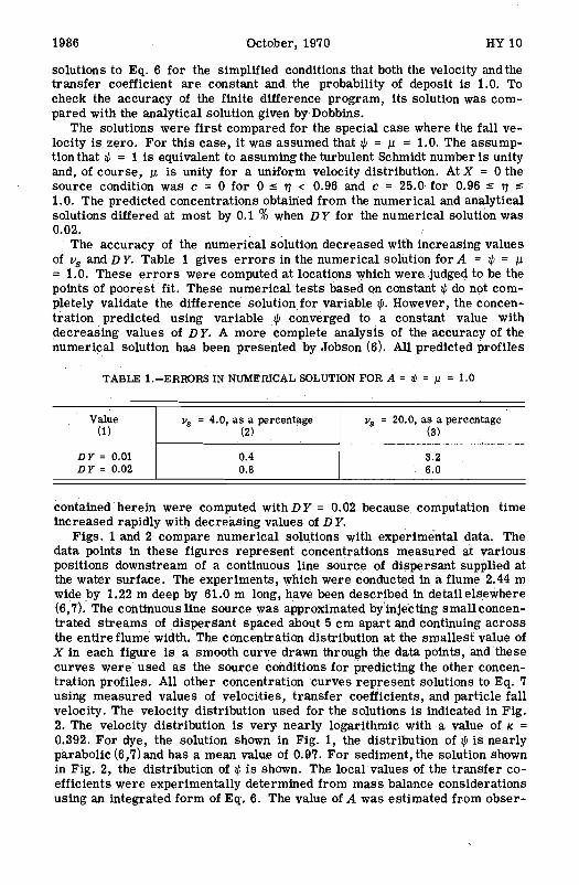
The accuracy of the numerical solution decreased with increasing values of v, and D Y. Table 1 gives e r r o r s in the numerical solution for A = $ = p = 1.0. These e r r o r s were computed a t locations which were judged to be the points of poorest fit. These numerical t es t s based on constant J , do not com- pletely validate the difference solution for variable J,. However, the concen- tration predicted using variable J , converged to a constant value with decreasing values of DY. A more complete analysis of the accuracy of the numerical solution has been presented by Jobson (6). All predicted profiles

TABLE 1.-ERRORS IN NUMERICAL SOLUTION FOR A = J, = p = 1.0

contained herein were computed wi thDY = 0.02 because computation time increased rapidly with decreasing values of D Y.

Figs. 1 and 2 compare numerical solutions with experimental data. The data points in these figures represent concentrations measured a t various positions downstream of a continuous line source of dispersant supplied at the water surface. The experiments, which were conducted in a flume 2.44 m wide by 1.22 m deep by 61.0 m long, have been described in detailelsewhere (6,7). The continuous line source was approximated by injecting smallconcen- trated s t r e ams of dispersant spaced about 5 cm apart and continuing across the entire flume width. The concentration distribution a t the smallest value of X in each figure i s a smooth curve drawn through the data points, and these curves were used a s the source conditions for predicting the other concen- tration profiles. All other concentration curves represent solutions to Eq. 7 using measured values of velocities, t ransfer coefficients, and particle fall velocity. The velocity distribution used for the solutions i s indicated in Fig. 2. The velocity distribution i s very nearly logarithmic with a value of K = 0.392. For dye, the solution shown in Fig. 1, the distribution of J , i s nearly parabolic (6,7) and has a mean value of 0.97. Fo r sediment, the solution shown in Fig. 2, the distribution of J , i s shown. The local values of the t ransfer co- efficients were experimentally determined from mass balance considerations using an integrated form of Eq. 6. The value of A was estimated from obser-

Value (1)

D Y = 0.01 D Y = 0.02

v, = 4.0, as a percentage (2)

0.4 0.8

V, = 20.0, as a percentage (3)

3.2 6.0

PREDICTING CONCENTRATION PROFILES 1987

o 29.0 cm/aac ~ a p t h of Flow = 4 0 . 3 cm 0 57.5 crn/sac n /u* = 6.38 0 8 8 5 cm/r*c

CONCENTRATLON

CONCENTRATION

FIG. 1.-COMPARISON OF SOLuTIbNS TO EQ. 6 WITH LABORATORY DATA FOR DYE

VELOCITY l u / U ) TRANSFER COEFFICIENT( Jr ) CONCENTRATION

CONCENTRATION

FIG. 2.-COMPARISON OF SOLUTIONS TO EQ. 6 WITH LABORATORY DATA FOR SEDIMENT

1988 October, 1970 HY 10

vations of the distribution of sediment on the floor of the flume following each run.

The ability of Eq. 6 to represent the physical process of vertical mass transfer in open channel flow i s demonstrated if it can reproduce measured concentrations atall stations for any values af p , J, and V, . The ability of Eq. 6 to represent the process of vertical mass transfer in open channel flow is shown in Figs. 1 and 2. In general, the deviation of the mean measured con- centration from the predicted concentration is less than the deviation between measured concentrations.

It was found that the numerical solution to Eq. 6 would not accurately pre- dict the first measured distributionfor any assumed source distribution which appeared consistent with the source distribution observed in the flume. Thus the first measured concentration distribution was used a s the source distri- bution in predicting the other distributions. The failure of Eq. 6 to represent the physical process near the source is not completely understood. However, the failure is believed to be due to one or a combination of the following: (1) Longitudinal concentration gradient 8 c / 8 ~ is not initially small; and (2) the concept of a gradient-type turbulent transfer coefficient, E , is not known to be valid until the thickness of the plume in the direction of transfer becomes larger than the eddies that are causing the transfer. Note the derivation of Eq. 6 required 8 c / 8 ~ << B C / B ~ and the value of cY be constant with respect to distance from the source.

EFFECTS OF HYDRAULIC PARAMETERS ON PmDICTED CONCENTRATIONS

In this section Eq. 6 will be numerically solved with differing hydraulic parameters in order to illustrate the interdependence and effects of these parameters on diffusion. The solution will be analyzed for the neutrally buoy- ant dye first (i.e. us = 0) and then the more complicated case, aparticulate dispersant, will be illustrated. The coupling relationship between the velocity profile and the turbulent transfer coefficient will be analyzed for each dispersant.

Neutrally Buoyant Dispersant.-From a known velocity and shear s t ress distribution in atwo-dimensional channel, the momentum transfer coefficient, E, , can be computed according to Boussinesq's definition:

in which rXy = the shearing stress acting parallel to the x coordinate on a surface normal to the y coordinate and p = the fluid density. Because the Reynolds' analogy, i.e., E, = ey, has been shown to be approximately true for a neutrally buoyant dye (1,5,7,8), it is instructive to compute some mo- mentum transfer coefficient distributions corresponding to various velocity distributions.

For wide open channels with essentially two-dimensional flow the shear stress distribution can be represented by

in which 7 , = the shear stress at the bed. Logarithmic equations such as

HY 10 PREDICTING CONCENTRATION PROFILES 1989

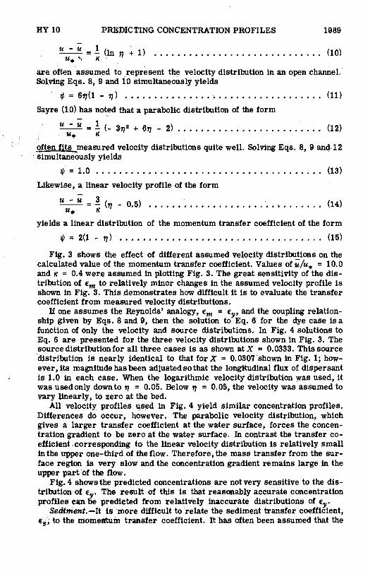
are often assumed to represent the velocity distribution in an open channel. Solving Eqs. 8, 9 and 10 simultaneously yields

Sayre (10) has noted that a parabolic distribution uf the form -

' often f i t smeasured velocity distributions quite well. Solving Eqs. 8, 9 and 12 , simultaneously yields

Likewise, a linear velocity profile of the form

yields a linear distribution of the momentum transfer coefficient of the form

Fig. 3 shows the effect of different assumed velocity distributions on the calculated value of the momentum transfer coefficient. Values of i / u , = 10.0 and K = 0.4 were assumed in plotting Fig. 3. The great sensitivity of the dis- tribution of em to relatively minor changes in the assumed velocity profile is shown in Fig. 3. This demonstrates how difficult i t is to evaluate the transfer coefficient from measured velocity distributions.

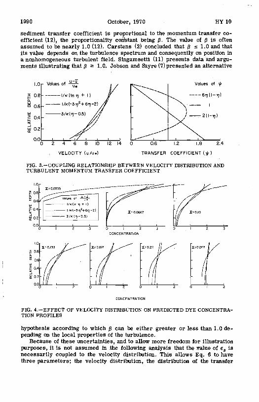
If one assumes the Reynolds' analogy, c, = cy, and the coupling relation- ship given by Eqs. 8 and 9, then the solution to Eq. 6 for the dye case is a function uf only the velocity and source distributions. In Fig. 4 solutions to Eq. 6 a re presented for the three velocity distributions shown in Fig. 3. The source distribution for all three cases is a s shown at X = 0.0333. This source distribution is nearly identical to that for X = 0.0307 shown in Fig. 1; how- ever, its magnitude has been adjusted so that the longwudinal flux of dispersant

, is 1.0 in each case. When the logarithmic velocity distribution was used, i t was usedonly downto g = 0.05. Below g = 0.05, the velocity was assumed to vary linearly, to zero a t the bed.

All velocity profiles used in Fig. 4 yield similar concentration profiles. Differences do occur, however. The parabolic velocity distribution, which gives a larger transfer coefficient a t the water surface, forces the concen- tration gradient to be zero a t the water surface. In contrast the transfer co- efficient corresponding t~ the linear velocity distribution is relatively small inthe upper one-third of the flow. Therefore,the mass transfer from the sur- face region is very slow and the concentration gradient remains large in the upper part of the flow.

Fig. 4 shows the predicted concentrations are not very sensitive to the dis- tribution of c . The result of this is that reasonably accurate concentration profiles can & predicted from relatively inaccurate distributions of cy:

Sediment.-It is more difficult to relate the sediment transfer coefficient, eS, to the momelvtum transfer coefficient. It has often been assumed that the

1990 October, 1970 HY 10

sediment transfer coefficient is proportional to the momentum transfer co- efficient (12), the proportionality cohtant being p . The value of p is often assumed to be nearly 1.0 (12). Carstens (2) concluded that p I 1.0 and that its value depends on the turbulence spectrum and consequently on position in a nonhomogeneous turbulent field. Singamsetti (11) presents data and argu- ments illustrating that 0 2 1.0. Jobson and Sayre (?)presented an alternative

Values of +

0 0.6 1.2 1.8 2.4

VELOCITY (u/u+) TRANSFER COEFFICIENT (.$ )

FIG. 3.-COUPLING RELATIONSHIP BETWEEN VELOCITY DISTRIBUTION AND TURBULENT MOMENTUM TRANSFER COEFFICIENT

CONCENTRATION

CONCENTRATION

FIG. 4.-EFFECT OF VELOCITY DISTRIBUTION ON PREDICTED DYE CONCENTRA- TION PROFILES

hypothesis according to which p can be either greater or less than 1.0 de- pending on the local properties of the turbulence.

Because of these uncertainties, and to allow more freedom for illustration purposes, i t is not assumed in the following analysis that the value of E, is necessarily coupled to the velocity distribution. This allows Eq. 6 to have three parameters; the velocity distribution, the distribution of the transfer

HY 10 PREDICTING CONCENTRATION PROFILES 1991

coefficient, and the fall velocity. In addition the boundary condition at the bed is more complex because it allows sediment to be either deposited on or de- flected upward from the bed.

The effects of varying the aforementioned parameters and the boundary condition on predicted sediment concentrations are shown in Figs. 5 through 8. The velocity distribution by itself was found to have a very minor effect on the predicted concentration. Thus only one velocity distribution, Eq. 10 with K = 0.4, is usedinthe solutions indicated in these figures. The magnitude and distribution of the sediment transfer coefficient ace varied independently of each other and of the velocity distribution. First, solutions are given using distributions of $ a s computed from Eqs. 11, 13 and 15 in which $ retains a constant mean value of 1.0. Next the effect of varying the average value of $ while keeping i ts distribution constant a s determined by Eq. 11 is shown. Then the effect of the fall velocity parameter, us, on diffusion is illustrated. Finally, the effect of the parameter, A , which controls the boundary condition at the bed on the predicted concentration profiles is shown.

For comparison, all figures (5 through 8) have one set of curves in common. This set of curves is shown a s solid lines and was determined using:

1. Velocity profile from Eq. 10 with K = 0.4. 2. $ = 6q( l - 7). 3. us = 3.0. 4. Probability of deposit, A = 0.3. 5. The source distribution at X = 0.05.

The source distribution is the same a s the measuredconcentration distribution occurring at X = 0.0493 shown in Fig. 2. This condition was used to avoid the problem of whether o r not Eq. 6 is valid close to the source. With the excep- tion of the parameter being shown, all parameters in Figs. 5 through 8 are held constant at the values given in the aforementioned listing.

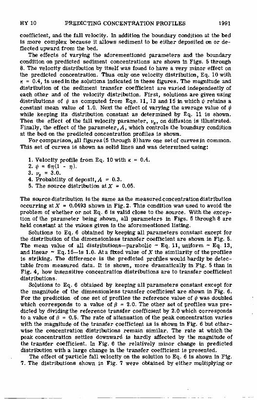
Solutions to Eq. 6 obtained by keeping all parameters constant except for the distribution of the dimensionless transfer coefficient are shown in Fig. 5. The mean value of all distributions-parabolic - Eq. 11, uniform - Eq. 13, and linear - Eq. 15-is 1.0. At a fixed value of X the similarity of the profiles is striking. The difference is the predicted profiles would hardly be detec- table from measured data. It is shown, more dramatically in Fig. 5 than in Fig. 4, how insensitive concentration distributions are to transfer coefficient distributions.

Solutions to Eq. 6 obtained by keeping all parameters constant except for the magnitude of the dimensionless transfer coefficient a re shown in Fig. 6. For the prediction of one set of profiles the reference value of $ was doubled which corresponds to a value of p = 2.0. The other set of profiles was pre- dicted by dividingthe reference transfer coefficient by 2.0 which corresponds to a value of p = 0.5. The rate of attenuation of the peak concentration varies with the magnitude of the transfer coefficient a s is shown in Fig. 6 but other- wise the concentration distributions remain similar. The rate at which the peak concentration settles downward is hardly affected by the magnitude of the transfer coefficient. In Fig. 6 the relatively minor change in predicted distribution with a large change in the transfer coefficient is presented.

The effect of particle fall velocity on the solution to Eq. 6 is shown in Fig. 7. The distributions shown in Fig. 7 were obtained by either multiplying o r

1992 October, 1970 HY 10

dividing the reference fall velocity parameter by 2. The rate of descent of the sediment mass is controlled mzinly by the particle fall velocity. As the flux of material to the bed is directly proportional to the fall velocity, see Eq. 4,

CONCENTRATION

FIG. 5.-'EFFECT OF TRANSFER COEFFICIENT DISTRIBUTION ON PREDICTED SEDIMENT CONCENTRATION PROFILES

CONCENTRATION

CONCENTRATION

FIG. 6.-EFFECT OF MAGNTTUDE OF TRANSFER COEFFICIENT ON PREDICTED SEDIMENT CONCENTRATION PROFILES

the amount of material left in suspension at large values of X is quite de- pendent upon the particle fall velocity. Comparing Figs. 6 and 7 one sees that the transfer coefficient and the fall velocity have quite different effects on the

HY 10 PREDICTING CONCENTRATION PROFILES 1993

predicted concentration profiles. Note that the fall velocity controls the rate of descent of the dispersant mass while hardly affecting the rate of spread of the dispersant. Conversely, the magnitude of the transfer coefficient controls

CONCENTRATION

CONCENTRATION

FIG. 7.-EFFECT OF PARTICLE FALL VELOCITY ON PREMCTED SEDIMENT CONCENTRATION PROFILES

CONCENTRATION

FIG. 8.-EFFECT OF BOUNDARY C ~ D I T I O N ON PREDICTED SEDIMENT CONCEN- TRATION PROFILES

the rate of spread of the dispersant mahls and the rate of attenuation of the maximum concentration but hardly affects the rate cJf descent of the dispers- ant mms. Because the position of the centroidof the dispersant mass is fairly

1994 October, 1970 HY 10

easily determined experimentally, the particle fall velocity can be determined fairly accurately from measured concentration profiles (6,7).

The effect of the probability of deposit, A, on the solution to Eq. 6 is shown in Fig. 8. The value of A significantly affects the profiles only near the bed. The fall velocity has a larger effect on the rate of deposit of material on the bed than does the value of A for the particular sets of conditions shown in Figs. 7 and 8. Note that for A = 0.0, no deposition on the bed, the concentra- tion gradient near the bed is very large. The results for A = 1.0 could be seen approximately by projecting the concentration profile forA = 0.6 to the bed such that 8c/87 = 0 at the bed.

SUMMARY AND CONCLUSIONS

An equation of two-dimensional mass transfer was solved numerically in order to illustrate the effects of the various parameters on vertical mass transfer. The numerical solution was checked for accuracy by comparison withthe analytic result obtained for a simplifiedcase. The solution was shown to adequately represent the physical process when compared with laboratory data obtained in a large flume. The effects of the various parameters and boundary conditions on mass transfer are shown in Figs. 4 through 8. The particle fall velocity controls the rate of descent of the dispersant mass but has little effect on the rate of spread of the dispersant. Conversely, the mag- nitude of the transfer coefficient controls the rate of spread of the dispersant but has little effect on its rate of descent. The most striking conclusion is that predicted concentration profiles are not very sensitive to the distribution of the vertical mass transfer coefficient.

ACKNOWLEDGMENT

This publication was authorized by the Director, U.S. Geological Survey.

APPENDIX I.-REFERENCES

I. Al-Saffar, Adnan Mustafa, "Eddy Diffusion and Mass Transfer in Open Channel Flow," thesis presented to the University of California, at Berkeley, Calif., in 1964, in partial fulfillment of the requirements for the degree of Doctor of Philosophy.

2. Carstens, M. R., "Accelerated Motion of a Spherical Particle," Transactions of the American Geophysical Union, Vol. 33, No. 5, Oct., 1952, pp. 713-720.

3. Dobbins, William E., "Effect of Turbulence on Sedimentation," Transactions, ASCE, Vol. 109, L

1944, pp. 629-667. 4. Fischer, H. B., "The Mechanics of Dispersion in Streams," Journal of the Hydraulics Division,

ASCE, Vol. 93, No. HY6, Proc. Paper 5592, Nov., 1967, pp. 187-216. 5. Hinze, J. 0.. Turbulence, McGraw-Hill Book Company, Inc., New York, N Y., 1959, pp.4-371. 6. Jobson, H. E., "Vertical Mass Transfer in Open Channel Flow," thesis presented to Colorado

State University at Fort Collins, Colo., in 1968, in partial fulfillment of the requirements for the degree of Doctor of Philosophy.

7. Jobson, H. E., and Sayre, W. W., "Vertical Transfer in an Open Channel Flow," Journal of the

HY 10 PREDICTING CONCENTRATION PROFILES 1995

Hydraulics Division. ASCE. Vol. 96, No. HY3, Proc. Paper 7148, Mar., 1970, pp. 703-724. 8. Pien, Chung Ling, "Investigation of Turbulence and Suspended Material Transportation in

Open Channels," thesis presented to The State University of Iowa at Iowa City, Iowa, in 1941, in partial fulfillment of the requirements for the degree of Doctor of Philosophy.

9. Richtmyer, R. D., "Difference Methods for Initial-Value Problems," Interscience Publishers, Inc., New York, N.Y., 1957, p. 237.

10. Sayre, W. W., "Dispersion of Mass in Open Channel Flow," Hydraulics Papers, NO: 3, Colorado State University, Fort Collins, Colo., Feb., 1968.

I I. Singamsetti, Surya Rao, "Diffusion of Sediment in a Submerged Jet," Journal o j the Hy- draulics Division. ASCE, Vol. 92, No. HY2, Proc. Paper 4726, Mar., 1966, pp. 153-168.

12.Task Committee, "Sediment Transportation Mechanics; Suspension of Sediment," Progress Report, Task Committee on Preparation of Sedimentation Manual Committee on Sedimenta- tion, Journal o j the Hydraulics Division. ASCE, Vol. 89, Pt. 1, No. HY5, Proc. Paper 3636, Sept., 1963, pp. 45-77.

APPENDIX 11. -NOTATION

The following symbols are used in this paper:

A = probability of deposit on flume floor; c = concentration of dispersant;

DX = longitudinal step = ~.O/M; DY = vertical step = ~.O/N;

E = dimensionless transfer coefficient 6 E/K YN u*; g = acceleration of gravity;

M = increments in horizontal per unit length used in numerical solution; N = increments in vertical used in numerical solution; S = slope of energy line; t = time;

Ul(i) = reciprocal of dimensionless velocity in ith row; u = local velocity in direction of mean flow;

ui = local velocity in ith coordinate direction;

u = depth averaged value of u; u, = shear velocity; VS = dimensionless fall velocity 6 V,/K u*; Vs = particle fall velocity in turbulent fluid; x = dimensionless distance from the source x = ( X K / [ ~ Y ~ ~ / U , ) ] ) ; x = coordinate distance along channel;

x i = ith coordinate direction; y = vertical coordinate distance;

YN = depth of flow; p = proportionality constant between E, and r,; y = specific weight of water; r1 = turbulent mass transfer coefficient in zYh direction;

r, = turbulent momentum transfer coefficient; eS = turbulent sediment transfer coefficient; - E = depth averaged value of c;

1996 Oatober, lev0

q = relative depth y / ~ N ; K a Von~Kacman~s turbulence _coeffiaient; p = difnensionleers velocity u/u;

us = dimensi6nless fall velocity 6 V*/K u,; p = density of water; T~ = boundary shear stress;

3 turbulent shear stress; and Ti$ = dlmensionlese transfer ooeifhi'ent' 6 t y / n Y N u .