BUDAPEST UNIVERSITY OF TECHNOLOGY AND ECONOMICS FACULTY OF MECHANICAL ENGINEERING DEPARTMENT OF POLYMER ENGINEERING DEVELOPMENT OF INJECTION MOLDABLE, THERMALLY CONDUCTIVE POLYMER COMPOSITES PHD THESIS ANDRÁS SUPLICZ MSC IN MECHANICAL ENGINEERING SUPERVISOR: JÓZSEF GÁBOR KOVÁCS, PHD ASSOCIATE PROFESSOR 2015
Transcript
BUDAPEST UNIVERSITY OF TECHNOLOGY AND ECONOMICS FACULTY OF MECHANICAL ENGINEERING DEPARTMENT OF POLYMER ENGINEERING
DEVELOPMENT OF INJECTION MOLDABLE , THERMALLY CONDUCTIVE POLYMER COMPOSITES
PHD THESIS
ANDRÁS SUPLICZ MSC IN MECHANICAL ENGINEERING
SUPERVISOR: JÓZSEF GÁBOR KOVÁCS, PHD
ASSOCIATE PROFESSOR
2015
András SUPLICZ
2
ACKNOWLEDGEMENTS
I would like to express my thanks to my supervisor, Dr. József Gábor KOVÁCS for
his help and support of my work and his guidance towards a deeper scientific way of thinking.
I also would like to say thank to Professor Tibor CZIGÁNY and Dr. Tamás BÁRÁNY, who
made me possible to work at the Department of Polymer Engineering. I would like to thank
the help and advices of Dr. Tamás TÁBI, Norbert Krisztián KOVÁCS and Ferenc SZABÓ. I
am also grateful to my colleagues and friends at the Department of Polymer Engineering for
their significant help and the creative atmosphere. I would also like to express my thanks to
my students who helped a lot with my work.
I express my thanks to the Hungarian Scientific Research Fund (OTKA PD105995)
for the financial support, to Arburg Hungary Ltd. for the Arburg Allrounder 370S 700-290
injection molding machine, to ANTON Kft. for the injection molds and to HSH Chemie Ltd.
for the free graphite sample.
This work is connected to the scientific program of the “Development of quality
oriented and harmonized R+D+I strategy and functional model at BME” project. This work is
supported by the New Széchenyi Plan (Project ID: TÁMOP-4.2.1/B-09/1/KMR-2010-0002).
The work reported in this thesis has been developed in the framework of the project
"Talent care and cultivation in the scientific workshops of BME" project. This project is
supported by the grant TÁMOP - 4.2.2.B-10/1-2010-0009.
Last, but not least I would like to express my thanks to my family and friends for their
unbroken support of my work.
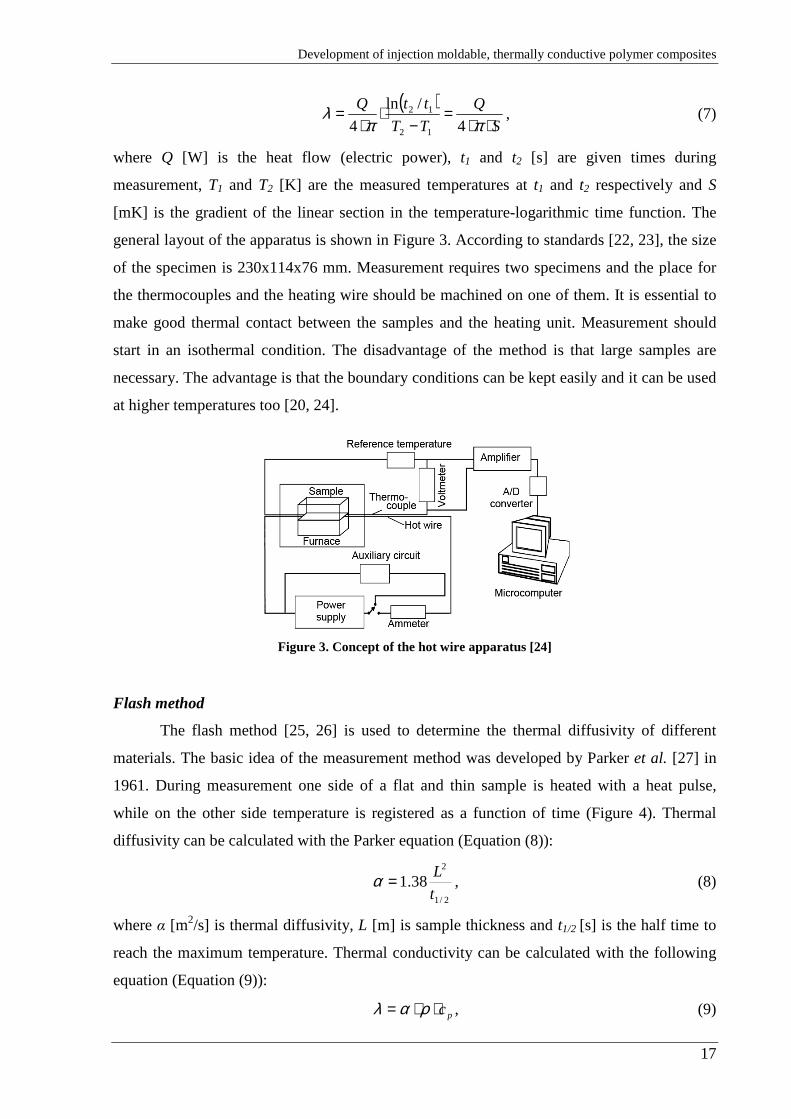
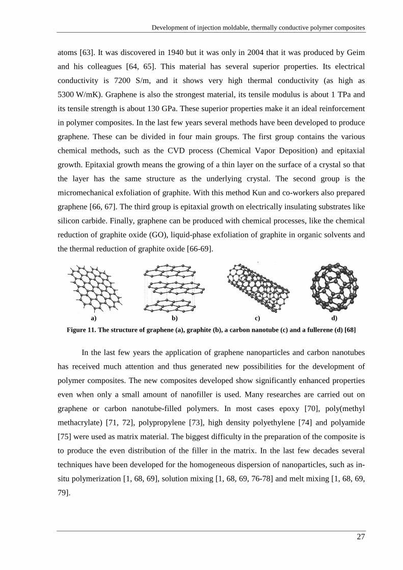
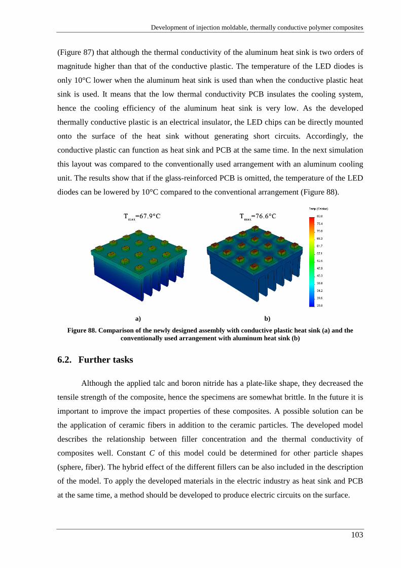
Development of injection moldable, thermally conductive polymer composites
(BN). The achievable thermal conductivity is influenced mainly by filler concentration,
particle size and shape, dispersion and surface treatment.
Lee et al. [93] investigated how the efficiency of solar cells can be enhanced by increasing the
thermal conductivity of the EVA (ethylene-vinylacetate) layer. A comprehensive study was
performed with many different types of filler, such as aluminum oxide, magnesium oxide,
zinc oxide, silicon carbide, boron nitride and aluminum nitride. The fillers were surface
treated with 1 m% silane. The samples were prepared by two-roll mill and compression
molding. The thermal conductivity (Figure 16) and also the electrical resistivity of the
composites were measured. The highest thermal conductivity, 2.85 W/mK was obtained with
60 vol% SiC. With 60 vol% ZnO and BN thermal conductivity was lower, 2.26 and 2.08
W/mK respectively, but the composites filled with these fillers showed better electrical
insulation.
Figure 16. Thermal conductivity of the EVA composites [93]
Ishida and Rimdusit [94] prepared a thermally conductive polymer composite by using
a polibenzoxazine matrix and boron nitride as filler (225 µm). The bisphenol-A-metilamin
Development of injection moldable, thermally conductive polymer composites
33
based polibenzoxazine has very low viscosity, which improves the wetting and dispersion of
the filler particles. The monomer and the BN was first dry mixed at room temperature then the
specimens were compression molded. In this way a very high, 78.5 vol% filler content was
achieved. Thermal conductivity was 32.5 W/mK.
Kemaloglu et al. [95] investigated the effect of micro and nano BN on the thermal,
mechanical and morphological properties of silicon rubber. 0, 10, 30 and 50 m% filled
composites were prepared with an extruder, then 1 and 3 mm thick samples were compression
molded. It was concluded that when BN was added to the matrix, tensile strength decreased in
all cases, which means that the interfacial interaction between silicone and BN is poor. It was
also stated that larger particle sizes resulted in worse mechanical properties. A similar effect
can be seen in the case of elongation at break. The tensile modulus increased with BN
content, and nano-sized BN has a more pronounced effect. On the other hand, particle size has
the opposite effect on thermal conductivity, and it was found that the aspect ratio of the filler
is critical in achieving high thermal conductivity. When 50 m% micro sized BN was added to
silicone rubber, the thermal conductivity was more than 2 W/mK.
Zhou [96] prepared thermally conductive linear low-density polyethylene (LLDPE)
composite with aluminum nitride (particle size: 8-10 µm; TC: 170 W/mK) as filler. The
composite was made on a two-roll mill up to 70 m% filler content and the samples were
prepared with compression molding. Zhou also prepared titanate-coated AlN powder.
According to Gu et al. [97] the titanate creates a monomolecular layer on the interface of AlN
and LLDPE. One end of the titanate coupling agent makes a strong chemical bond with the
free protons on the AlN surface, and the van der Waals force links the other end of the
coupling agent to the LLDP chains. The DSC measurements showed that as the AlN content
was increased, the crystallinity of the composite decreased. According to Luyt et al. [98], the
main reason is that LLDPE has relatively high crystallinity and has no bigger amorphous
phase where the crystals could be placed. Hence at low filler content the AlN particles are in
the interlaminar layers, which blocks further crystal evolution. At higher filler content there is
a change in crystal evolution. Thermogravimetry analysis (TGA) showed that there is a
significant increase in the thermal stability of LLDPE with increasing AlN concentration. The
explanation can be the higher heat capacity and the high thermal conductivity, which cause an
improved heat absorption ability. In this manner LLDPE chains start to degrade at higher
temperatures. According to thermal conductivity measurements, at 70 m% (~40 vol%) AlN
and titanate modified AlN concentration the thermal conductivity of the composites is 1.25
and 1.39 W/mK, respectively. The temperature dependence of thermal conductivity was also
András SUPLICZ
34
investigated between 25 and 120°C. It was found that by increasing the temperature, thermal
conductivity decreases, which is caused by thermal expansion. As a consequence of thermal
expansion the distance between the AlN particles in the LLDPE matrix starts to increase.
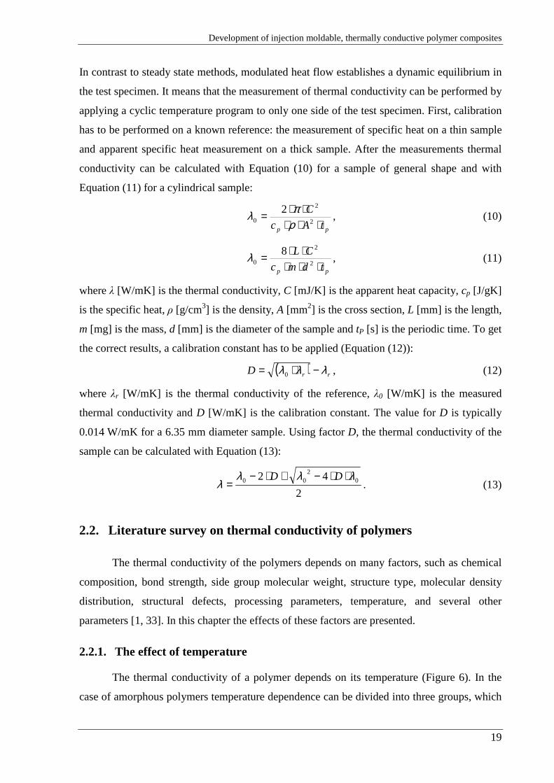
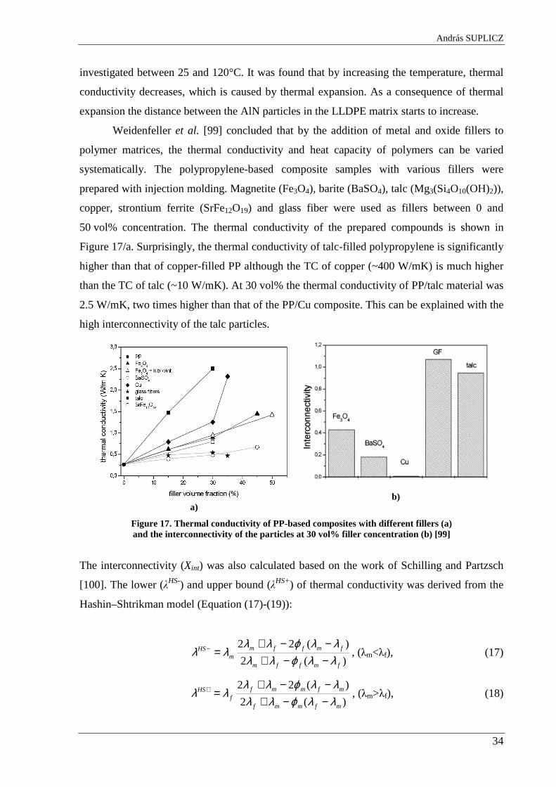
Weidenfeller et al. [99] concluded that by the addition of metal and oxide fillers to
polymer matrices, the thermal conductivity and heat capacity of polymers can be varied
systematically. The polypropylene-based composite samples with various fillers were
prepared with injection molding. Magnetite (Fe3O4), barite (BaSO4), talc (Mg3(Si4O10(OH)2)),
copper, strontium ferrite (SrFe12O19) and glass fiber were used as fillers between 0 and
50 vol% concentration. The thermal conductivity of the prepared compounds is shown in
Figure 17/a. Surprisingly, the thermal conductivity of talc-filled polypropylene is significantly
higher than that of copper-filled PP although the TC of copper (~400 W/mK) is much higher
than the TC of talc (~10 W/mK). At 30 vol% the thermal conductivity of PP/talc material was
2.5 W/mK, two times higher than that of the PP/Cu composite. This can be explained with the
high interconnectivity of the talc particles.
a)
b)
Figure 17. Thermal conductivity of PP-based composites with different fillers (a) and the interconnectivity of the particles at 30 vol% filler concentration (b) [99]
The interconnectivity (Xint) was also calculated based on the work of Schilling and Partzsch
[100]. The lower (λHS-) and upper bound (λHS+) of thermal conductivity was derived from the
Hashin–Shtrikman model (Equation (17)-(19)):
)(2
)(22
fmffm
fmffmm
HS
λλϕλλλλϕλλ
λλ−−+−−+
=− , (λm<λf), (17)
)(2
)(22
mfmmf
mfmmff
HS
λλϕλλλλϕλλ
λλ−−+−−+
=+ , (λm>λf), (18)
Development of injection moldable, thermally conductive polymer composites
35
−+
−
−−
=HSHS
HS
Xλλ
λλ0int . (19)
In the equations λm and λf are the thermal conductivity of the matrix and fillers, and φf and φm
are the filler and matrix concentration by volume. The results are shown in Figure 17/b. It can
be clearly seen that talc and glass fiber form the best interconnected network through the
matrix.
Droval et al. [101] investigated the properties of BN, talc, aluminum nitride and
aluminum oxide filled polystyrene conductive composites. The fillers were investigated with
scanning electron microscope (SEM) and it was found that the BN and talc particles have a
plate-like shape, while AlN and Al2O3 particles have a spherical shape. Boron nitride was
found to be the most effective filler offering a good compromise between high intrinsic
thermal conductivity, a high shape factor and high connectivity. The DSC measurements
showed that the glass transition temperature of PS decreases as filler fraction is increased. BN
had the most pronounced, at 10 vol% Tg decreased by 15°C. In the case of other fillers this
decrease was less than 8°C. The results of thermal conductivity measurements are presented
in Figure 18. It can be clearly seen that the thermal conductivity of the PS/BN composite is
about twice as high as that of the other composites.
Figure 18. The thermal conductivity of polystyrene-based composites as a function of filler concentration [101]
András SUPLICZ
36
2.3. Modeling methods on thermal conductivity
In this chapter the most important basic and advanced models used for the prediction
of thermal conductivity of composites are introduced. Besides the mathematical models, some
authors presented Finite Element Modeling methods to estimate the conductivity of the
composites as a function of filler concentration.
2.3.1. Numerical methods
To keep the price of polymer composites as low as possible, it is important that their
properties can be tailored to needs. Hence it is important that the composite can be designed
using the proper type and ratio of the matrix and fillers [87]. However, not only mechanical,
but also thermal properties, such as thermal conductivity should be predictable. The thermal
conductivity of composite materials is influenced by several factors, such as filler
concentration, particle size and shape, filler dispersion and distribution in the matrix, the
thermal conductivity of the components, the contact between the particles and the contact
surface resistance between the matrix and the filler [1, 87]. Although numerous empirical,
semi-empirical and theoretical models have been developed for the prediction of thermal
conductivity of two- or multiphase polymer composites, its reliable and precise prediction still
remains a challenge. The three basic models are the rule of mixtures (parallel model), the
inverse rule of mixtures (series model) and the geometric mean model. In the rule of mixtures
(Equation (20)) it is assumed that the components contribute to the thermal conductivity of
the composite proportionally. It generally overestimates the experimental values and provides
an upper bound for conductivity. This model assumes the existence of a percolation network
of the filler in the matrix and perfect contact between the filler particles. On the other hand,
the inverse rule of mixtures (Equation (21)) assumes that there is no contact between the
particles, thus it underestimates the experimental values and provides a lower bound for
conductivity:
mmffc ϕλϕλλ += , (20)
m
m
f
f
c λϕ
λϕ
λ+=1
, (21)
where λc is the thermal conductivity of the composite, λm and λf are the thermal conductivity
of the matrix and the filler, and φf is the filler fraction. The geometric mean model
(Equation (22)) is an empirical method for the prediction of the thermal conductivity of
Development of injection moldable, thermally conductive polymer composites
37
composites. It provides better results than the rule of mixtures and inverse rule of mixtures [1,
102, 103].
)1( ff
mfcϕϕ λλλ −⋅= . (22)
Besides these basic models, many advanced models have been developed. The most
important theoretical equations are the Maxwell [104], Bruggeman [102], Cheng-Vachon
[105], Hamilton-Crosser [106] and Meredith-Tobias [107] model. Maxwell (Equation (23))
supposed that spherical filler particles are randomly distributed in the matrix and there is no
interaction between them. This model describes the thermal conductivity of composites with a
low volume fraction of fillers well, but as filler content is increased, the particles start to
develop interactions between each other and form conductive chains [102, 104, 108, 109].
)](2[
)](22[
mfffm
mfffmmc λλϕλλ
λλϕλλλλ
−⋅−+⋅−⋅⋅++⋅
⋅= . (23)
Bruggeman developed another theoretical model. This implicit relation (Equation (24)) also
supposes that the spherical, non-interacting particles are homogeneously dispersed in the
continuous matrix [87, 102, 108, 109].
( )
)(
)(1
3/1
mf
cmcff λλ
λλλλϕ
−−⋅−
=− . (24)
Cheng and Vachon [105] developed another theoretical model (Equation (25) and
(26)) for two-phase composite materials. This equation assumes that the discontinuous phase
has a parabolic distribution in the continuous matrix. The parabolic distribution constants (Bcv
and Ccv) were introduced and related to the volume fraction of the filler [102, 105, 110, 111].
m
cv
fmcvcvmfcvm
fmcvcvmfcvm
mfcvmfmcvc
B
CBB
CBB
BC
λλλλλλλλλλλ
λλλλλλ
−+
−⋅−−+
−⋅+−+⋅
−+⋅−=
1
)(2/)(
)(2/)(ln
)(()(
11
, (25)
2
3 fcvB
ϕ⋅= ,
fcvC
ϕ⋅⋅−=
3
24 . (26)
On the other hand, there are numerous empirical and semi-empirical models that
contain experimental factors for thermal conductivity and for the volume fraction of the
components. Agari and Uno [112] and Lewis and Nielsen [113] developed such models, for
example. These models also show good correlation with the experiments up to 30 vol% filler
content. Only the Lewis-Nielsen model gives better fit above 30 vol%, thanks to the
introduction of the maximum volume fraction of fillers in the equation [1, 102].
András SUPLICZ
38
The Agari and Uno [112] model is based on the generalization of series and parallel
conduction models. It assumes that the particles form conductive chains through the matrix.
Accordingly, the thermal conductivity of two-phase composites can be written according to
Equation (27):
)log()1(loglog 12 mfffc CC λϕλϕλ ⋅⋅−+⋅⋅= , (27)
where λc, λf and λm are the thermal conductivity of the composite, the filler and the matrix, φf
is the filler volume fraction and C1, C2 are experimental constants. C1 is dedicated to the
effect of filler particles on the secondary structure of the polymer matrix (crystallinity, crystal
size) and C2 shows the conductive chain formation ability of the particles. Lewis and Nielsen
[114] reported a semi-empirical model, which was developed on the basis of the Halpin-Tsai
[115] equation. In this model the effect of particle shape, the orientation of the particles and
the packing of the fillers are included (Equation (28) and (29)):
−+
=ϕψ
ϕλλ
B
BA fLNLNmc 1
1, (28)
LNmf
mfLN A
B+
−=
)/(
1)/(
λλλλ
, f
m
m ϕϕ
ϕψ ⋅
−+=
2
11 , (29)
where λc, λf and λm are the thermal conductivity of the composite, the filler and the matrix, φf
is the filler volume fraction, ALN is a constant that depends on the shape and orientation of the
particles and φm is the maximum packing fraction of the filler. The values of ALN and φm were
determined for several filler types and orientation and can be found in tables. As an example,
for spherical particles, ALN =1.5 and φm=0.637 and for randomly packed irregularly shaped
particles ALN =3 and φm=0.637.
From the literature survey it is obvious that the exact prediction of thermal
conductivity for highly filled composites still poses difficulties. The theoretical models often
underestimate the results and can be used only up to 30 vol% filler content [108, 109, 111,
116, 117]. The semi-empirical models give better correlation with the experiments, but they
need more experimental parameters.
Kumlutas and Tavman [86] compared the thermal conductivity of HDPE/tin
composites to the results from some mathematical models. They found that all the models
used are in good agreement with the measured values at low filler content, except the Cheng-
Vachon model. At higher filler fractions (>10 vol%) the particles form conductive chains and
the gradient of the curves start to increase more rapidly. This range can be described with the
Cheng-Vachon and Agari-Uno models (Figure 19).
Development of injection moldable, thermally conductive polymer composites
39
Figure 19. Experimental and theoretical thermal conductivity of HDPE/tin composites [86]
Droval et al. [101] analyzed the thermal conductivity of more ceramic-filled (BN,
Al 2O3, AlN, talc) PS composites and compared it to the predicted values from theoretical,
empirical and semi-empirical models. They stated that the Cheng-Vachon, Lewis-Nielsen and
Agari-Uno model have a good correlation with the experiments and the Maxwell model can
be used only at low filler fractions (Figure 20).
Figure 20. Measured and modeled thermal conductivity of PS/BN composites [101]
The authors also calculated the interconnectivity coefficient of the fillers (Equation 19) in the
composites based on the work of Weidenfeller et al. [99]. They found that in a PS matrix talc
particles have the best interconnectivity, BN and Al2O3 have the same effect, and AlN has the
worse interconnectivity factor (Figure 21).
András SUPLICZ
40
Figure 21. The interconnectivity factor of the fillers in a PS matrix [101]
Dey and Tripathi [87] used several mathematical models to predict the filler
concentration dependent thermal conductivity of HDPE/Si composites between 0 and 20
vol% Si fractions. The Agari-Uno and Lewis-Nielsen models seem to correlate best with the
experiments. The experimental and modeled results can be seen in Figure 22/a and the
calculation error of the models in Figure 22/b.
a)
b)
Figure 22. Experimental and modeled thermal conductivity of HDPE/Si composites (a) and the calculation error of the Agari and Lewis models (b) [87]
It is well-known that nanoparticles easily form networks even in low concentration,
which can be proved by the electrical conductive chains above the percolation threshold.
Although there is no rapid increase in thermal conductivity at this threshold, the percolation
model is generally used to predict the thermal conductivity of carbon nanotube-filled
polymers. Foygel et al. [118] estimated the parameters of a percolation model with
simulations. This Percolation model is presented in Equation (30).
[ ] )()();(
rat
rpftrf aaλϕϕλϕλ −= , (30)
Development of injection moldable, thermally conductive polymer composites
41
where λ is thermal conductivity, λt is a factor that takes into consideration the thermal
conductivity of nanotubes and their contacts with each other, φf [vol%] is filler concentration,
φp [vol%] is the percolation threshold, ar is the aspect ratio of fillers and tλ is a factor that
characterizes the conductive chain. The value of λt is between 64 and 137 W/mK according to
the experiments. Haggenmueller et al. [119] investigated the percolation model on
HDPE/SWCNT nanocomposites. It was stated that the percolation model has a good
correlation with the experiments up to 20 vol% (Figure 22).
Figure 23. Comparison of the experimental values (dots) and percolation model (line) for HDPE/SWCNT nanocomposites [119]
2.3.2. Finite element modeling method
In addition to the mathematical models, numerous studies exist on the finite element
modeling (FEM) of composites and the calculation of their effective thermal and mechanical
properties. In cases when a problem cannot be solved analytically, FEM and simulation can
be effective methods. A considerable obstacle to the use of this method can be complicated
material arrangement, proper mesh generation and computational cost [120].
Kumlutas and Tavman [86] numerically modeled the thermal conductivity of polymer
composites. The models of particle-filled composites are cubes in a cube and spheres in a
cube lattice array (Figure 24). The ANSYS finite-element program was used for the
calculations. The results were compared to the experimental results of tin particle (0-16 vol%)
filled HDPE. It was found that up to 10 vol% tin the numerical model estimated thermal
conductivity well. Above 10 vol% the model underestimates the experiments.
András SUPLICZ
42
a)
b)
Figure 24. Sphere in cube (a) and cube in cube (b) three-dimensional finite element models for ANSYS simulations [86]
Mortazavi et al. [121] investigated and numerically simulated the thermal conductivity of an
expanded graphite-filled (EG) polylactic acid (PLA) composite. In the simulation model the
filler particles are randomly distributed in the matrix (Figure 25). The analyses were carried
out with the ABAQUS simulation software. It was found that the simulation results are in
good agreement with the experiment, although filler content was varied only between 0 and
6.75 wt%.
a)
b)
Figure 25. 3D model (a) and meshed model (b) of a PLA/EG composite [121]
Li et al. [122] developed a three-dimensional computational model using the finite
element method based on continuum mechanics. With the proposed model they evaluated the
thermal behavior of randomly distributed SWCNT/polyolefin and SWCNT/epoxy
composites. The 3D model was generated with a program developed in-house, and the 3D
tetrahedral elements were generated with the ANSYS software (Figure 26). To reduce the
computational costs, some simplifications were made regarding the shape, aspect ratio and
properties of SWCNTs. The authors analyzed the effects of interfacial thermal resistance,
volume fraction, thermal conductivity and the diameter of SWCNTs on the thermal
Development of injection moldable, thermally conductive polymer composites
43
conductivity of the composite. It was found that the model can be applied up to 10 vol%.
Above 10 vol% the error of prediction can be explained with the simplification of the model
and with the agglomeration of particles.
a)
b)
Figure 26. Model for three-dimensional randomly distributed SWCNT in a polymer matrix (a) and the discretized model with tetrahedral elements (b) [122]
Nayak et al. [123] constructed a three-dimensional spheres-in-cube lattice array model
to simulate the structure of epoxy/pinewood dust composite materials for filler concentrations
between 6 to 36 vol%. In the model the thermal conductivity of composites were numerically
analyzed with ANSYS and compared to experimental values and to other theoretical and
experimental models. It was concluded that the FEM analysis is more accurate than the rule of
mixture or the Maxwell model.
András SUPLICZ
44
2.4. Summary of the literature, objectives of the dissertation
The aim of the literature survey was to show the possibilities of application and
development of thermally conductive polymers. At the beginning the theory and physics of
thermal conductivity and its measurement methods were reviewed. Next, methods to improve
thermal conductivity were surveyed, such as the effect of molecular orientation, crystallinity,
processing methods and additives. According to the literature, the best method is the use of
fillers. Hence the three main groups of fillers (metallic, ceramic and carbon-based fillers)
were analyzed. It was also concluded that fillers can significantly influence the flow
properties of polymers. Moreover, a segregation effect can develop during the production of
the parts, which can influence the thermal and mechanical properties of the composites.
The thermal conductivity of polymers can be modified in many ways. If the
crystallinity of the polymers is increased, thermal conductivity also increases. This statement
can prove that fact that amorphous polymers have lower thermal conductivity than semi-
crystalline polymers. Research shows that the molecular weight also has a significant
influence; polymers with higher molecular mass also have higher thermal conductivity. The
orientation of the polymer chains can improve conductivity as well, but the material will be
anisotropic. Thermal conductivity increases in the direction of the orientation and decreases
perpendicular to that. These methods only have a slight effect on thermal conductivity. The
best results can be obtained with the use of solid fillers, which was proved by many
researchers. Metallic and carbon-based fillers are the best for this purpose, but the composite
will also be an electrical conductor. As the goal of this research is to produce dielectric
polymer composites of high thermal conductivity, these fillers can be applied up to the
percolation threshold. In contrast, ceramic fillers have better properties, such as good thermal
conductivity, low density and good electrical insulating properties.
In the literature, many different results can be found for the same type of fillers or
matrices. These differences can be attributed to the different measuring methods or different
processing methods. Many different measuring techniques exist, such as the hot plate, hot-
wire, laser flash methods and others, and these methods work on different principles.
Accordingly, the results may be different but the different measurement principles cannot
explain the huge deviations. To analyze the effect of different processing methods and
processing parameters is essential to understand their effect on filler distribution within the
matrix. Hence the segregation effect could not be neglected. Segregation can be through the
Development of injection moldable, thermally conductive polymer composites
45
thickness (shell-core effect) and along the flow length. Segregation can decrease the thermal
conductivity of the part and cause inhomogeneity regarding the thermal and mechanical
properties. Therefore this effect should be investigated.
In most articles the authors only used a single filler to produce conductive compounds.
Generally these fillers were copper, carbon black, graphite, carbon nanotubes, silicon dioxide,
talc, aluminum nitride and boron nitride. Only a few articles investigated polymer composites
with a hybrid filler system. In these papers at least one of the fillers is an electrical conductor,
such as carbon black or graphite. So far I have not found any articles applying only dielectric
fillers to utilize the advantages of the hybrid effect between different fillers.
It is important that the thermal conductivity of polymer composites should be tailored
to requirements. As was shown earlier, the thermal conductivity of composite materials is
influenced by several factors, which should be taken into account. Although numerous
empirical, semi-empirical and theoretical models have been developed for the prediction of
the thermal conductivity of two- or multiphase polymer composites, its reliable and precise
prediction still remains a challenge. From the literature survey it is obvious that the exact
prediction of thermal conductivity for highly filled composites still poses difficulties. The
theoretical models often underestimate the results and can be used only up to 30 vol% filler
content. The semi-empirical models give better correlation with the experiments, but they
need more experimental parameters.
Improving thermal conductivity with solid fillers can cause difficulties in material
processing. The viscosity of the polymer increases drastically as filler concentration is
increased. Generally, in the literature conductive polymer composites with a thermoplastic
matrix were prepared with internal mixing and compression molding, or simply a low
viscosity thermosetting matrix was used. These techniques are too slow for mass production
and can compromise design freedom. On top of that, only a few articles were published on the
injection molding of thermally conductive polymers, therefore this is a new area to
investigate.
Also, only a few articles can be found on the thermal properties of highly filled
polymers and so there is not much information on the influence of fillers on the glass
transition temperature and the crystallinity of thermally conductive polymers.
András SUPLICZ
46
Based on the literature survey, I have set out the following objectives of this PhD
dissertation:
1. The development and investigation of a novel thermally conductive polymer, which is
an electrical insulator.
2. The investigation of the effects of different parameters (matrix, filler, processing
technology, etc.) on the effective thermal conductivity of polymer composites.
3. The development of a polymer composite with a dielectric hybrid filler system to
enhance effective thermal conductivity with the same amount of filler.
4. The investigation of the thermal properties and crystallinity of conductive polymers,
influenced by the injection molding process.
5. The improvement of processability of highly filled polymers.
6. The development of a model to predict the thermal conductivity of composites as a
function of filler concentration.
Development of injection moldable, thermally conductive polymer composites
47
3. Materials and methods
In this chapter the selected materials, their processing methods and the testing methods
are introduced.
3.1. Materials
In my research composites were prepared with the use of different matrices and fillers.
The names, manufacturers and abbreviations (used in my research) of the applied materials
are presented in Table 1 and Table 2. Talc, boron nitride and graphite have plate like shape
which show anisotropic behaviors (Figure 27/a, b, d). The titanium dioxide has spherical
shape (Figure 27/c). The matrices can be processed directly, only polyamide 6 and polylactic
acid need to be dried at 80°C for 4 hours.
Name Trade name Manufacturer Abbreviation in the dissertation
Polypropylene homopolymer
Tipplen H 145 F Tisza Chemical Group
Public Limited Company PP
Polypropylene copolymer
Tipplen K 693 Tisza Chemical Group
Public Limited Company cPP
Polyamide 6 Schulamid 6 MV 13 A. Schulman, Inc. PA6
Residual cooling time [s] 10 Zone temperatures [°C] 200; 195; 190; 185; 180 Mold temperature [°C] 50
Table 4. Injection molding parameters
3.3. Testing methods
The samples for thermal, mechanical and morphological investigation were cut from
the 2 mm thick plates with a water jet cutter machine. On these specimens mechanical,
thermal and morphological analyses were performed. The details of the testing methods are
presented in this section.
Mechanical tests
Tensile testing
The tensile tests were carried out according to the recommendation of the
ISO 527-1:2012 standard [125] with a Zwick Z020 universal testing machine. The type of the
standard specimen was 5A (length: 75 mm, width: 4 mm, thickness: 2 mm, grips length:
50 mm). The testing speed was 2 mm/min. The tests were performed at room temperature
(25°C). From the force-displacement curves the tensile strength (σ [MPa]) and tensile
modulus (E [MPa]) of the samples were calculated. The tensile strength was determined from
the maximum developed force. The tensile modulus was calculated between 0.0005 and
0.0025 strain. The tensile properties were determined from five measurements in each case.
Development of injection moldable, thermally conductive polymer composites
51
Charpy impact testing
The Charpy tests were carried out according to the recommendation of the
ISO 179-2:1997 standard [126] with a Ceast Resil Impactor Junior machine. For the tests
unnotched specimens with a 2x6 mm cross-section were used with a 40 mm span distance.
The tests were performed at room temperature with a 2 J pendulum. From the absorbed
energy the Charpy impact strength (acU [kJ/m2]) could be calculated. The impact properties
were determined from ten measurements in each case.
Thermal analysis
Thermal conductivity
The thermal conductivity of the composite samples was measured with two different
methods: the hot plate (applied for the measurements in Chapter 5.1-5.3) and the linear heat
flow method (applied for the measurements in Chapter 5.4). Apparatuses were developed for
the measurements; they are presented in Chapter 4.
DSC analysis
A DSC Q2000 (TA Instruments) differential scanning calorimeter was used to analyze
the specific heat, crystallization temperature and crystallinity of the samples. 3-5 mg samples
were cut off from the center of the injection molded plates and placed into pans. The
measurements consisted of three phases: heating to 225°C from 25°C, cooling back to 25°C
and heating to 225°C again. The first heating is used to measure the effect of the injection
molding process, as in the next two phases crystals are created and melted during a controlled
process (at a heating and cooling rate of 10°C/min). The degree of crystallinity (X) was
determined from the exothermic and the endothermic peaks with Equation (33), which takes
into account the filler fraction of the compound [127]:
)1( ϕ−⋅∆
∆−∆=
f
ccm
H
HHX , (33)
where ∆Hm is the enthalpy of melting, ∆Hcc is the enthalpy of cold crystallization, ∆Hf is the
melting enthalpy of a theoretically fully crystalline polymer and φ is the mass fraction of the
filler. For the calculations the ∆Hf is 165 J/g [128] and 93 J/g [129] at the case of
polypropylene homopolymer and polylactic acid respectively.
András SUPLICZ
52
Microscopy
The fracture surface of the samples was analyzed with a Jeol JSM 6380LA Scanning
Electron Microscope. The samples were first coated with an Au/Pd alloy with a Jeol JFC-
1200 fine coater apparatus to avoid electric charging.
Segregation investigation
To determine filler distribution in the injection molded samples, they were cut into 16
identical parts, as can be seen in Figure 29. Next, the density of the samples was measured
based on Archimedes' principle.
Figure 29. Sample preparation for the investigation of segregation
Knowing the density of the matrix, the filler and the composite, the filler and matrix
concentration can be calculated according to the Equations (34) and (35):
100⋅−−
=mf
mcf ρρ
ρρϕ , (34)
fm ϕϕ −= 100 , (35)
Flow properties
Melt volume rate measurements
To characterize the flow properties of the materials, the melt volume rate (MVR) was
determined according to the ISO 1133-1:2013 [130] standard at 230°C, with a load of 2.16 kg
using CEAST Modular Melt Flow (7027.000) apparatus. In each case 6 measurements were
performed. The measurement procedure consists of the following steps: 60 seconds
preheating; compacting with 375 N to the position of 75 mm; compacting with the standard
(2.16 kg) weight; and performing a measurement at 40, 30 and 20 mm.
Development of injection moldable, thermally conductive polymer composites
53
Viscosity measurement
The viscosity of the CBT modified polypropylene was measured with an Instron
capillary rheometer, installed on a Zwick Z050 tensile-testing machine. Measurements were
made at four different temperatures: 190, 200, 220 and 240°C, with three capillaries of
different length (Table 5) and at seven different crosshead speeds: 5, 10, 20, 50, 100, 200 and
500 mm/min. The details of the calculations and corrections are presented in Chapter 5.3.
Nr. Sizes of the capillaries
Diameter [mm]
Length [mm]
1 1.23 24.45 2 1.20 49.17 3 1.20 73.55
Table 5. Sizes of the capillaries used for the viscosity measurements
András SUPLICZ
54
4. Development of heat conductometers
To measure the thermal conductivity of the composite samples, two different thermal
conductometers were developed, a hot plate and a linear heat flow apparatus. In this section
the basic theory and layout of these units are presented.
4.1. Hot plate apparatus
In this research a single-specimen hot plate apparatus was developed. In contrast to the
conventional two-specimen apparatus, heat flows in a single direction between the hot plate
and the cold plate through the specimen. Furthermore, in this arrangement a cold plate, a hot
plate and a specimen can be omitted, thus the apparatus is simpler. Figure 30 shows the main
components of the designed measurement system.
Figure 30. Main components of the hot plate apparatus
The main task is to maintain the temperature difference between the cold and the hot plates.
The thermal conductivity of the applied copper plates is ~380 W/mK, which is two orders of
magnitude higher than that of the samples, thus their heat resistance does not generate a
significant error. The cold plate of the apparatus was cooled by four 40x40 mm sized Peltier
cells, which facilitated keeping the temperature of the plate more precisely. The upper plate
was heated by a heating wire, where the generated heat is equal to the electrical energy
flowing through the wire (with losses ignored). To provide uniform heating of the hot plate,
the heating wire was meander-shaped. The heat resistance between the components was
decreased with thermally conductive tape (3M 8805). The temperature was measured with
two built-in NTC thermistors (Epcos B57045K) inside both the heated and the cooled plate.
Development of injection moldable, thermally conductive polymer composites
55
The resistance-temperature calibration for the NTC thermistors was performed with the
Steinhart-Hart equation (Equation (36)) [131]:
3))(ln()ln(1
RCRBAT SHSHSH ++= , (36)
where R [Ω] is the resistance of the thermistors at given temperatures T [K], and ASH, BSH and
CSH are the Steinhart-Hart constants. Table 6 contains the values of the Steinhart-Hart
constants obtained by calibration. The whole measurement system was controlled with a
programmed microcontroller (ATMEGA64). The scheme of the thermal conductometer
control system can be seen in Figure 31.
Thermistor no. A B C
1 2.569·10-3 7.035·10-5 1.838·10-6
2 2.378·10-3 6.785·10-6 1.180·10-6
3 1.847·10-3 8.564·10-5 9.509·10-7
4 1.693·10-3 1.239·10-4 6.663·10-7
Table 6. Steinhart-Hart constants of the thermistors
ATX, PSUcontrol
Temperaturemeasurement
Cold platetemperatureregulation
Hot platetemperatureregulation
USBconnection
to PC
Microcontroller
Figure 31. Scheme of the thermal conductometer control system
To reduce heat loss, the apparatus was thermally insulated with polystyrene foam, whose
thermal conductivity is ~ 0.04 W/mK. To decrease the thermal resistance between the samples
and the hot plate apparatus, thermal interface silicone grease was applied. To control the input
parameters for the measurement, such as heating power, the temperature of the cold plate and
the size of the specimen, a computer program was written. Using the input and output
parameters the program can also calculate thermal conductivity. Finally the apparatus was
calibrated with samples of known conductivity.
András SUPLICZ
56
4.2. Linear heat flow apparatus
A further thermal conductivity meter was designed and built, based on the
Comparative Longitudinal Heat Flow method [132, 133]. In this method the unknown sample
is compressed between the known reference samples and a heat flux passes through the
measurement unit as a temperature difference is created between the two sides of the unit. The
thermal conductivities of the sample and the reference sample are inversely proportional to
their thermal gradients. The apparatus developed (Figure 32) contains two C10 steel
(55 W/mK) cylinders with a diameter of 30 mm; and a length of 30 mm. A specimen of a
diameter of 30 mm and a thickness of 10 mm is placed between the steel cylinders. On the
contact surface thermal grease was applied to decrease heat resistance. 3 thermocouples were
inserted in each cylinder to detect temperature: one 3 mm below the top, one in the middle
and one 3 mm above the bottom (Tm1-Tm6/Figure 32). The temperatures were registered with
an Ahlborn Almemo 8990-6-V5 data acquisition module with a resolution of 0.1°C. The
apparatus was clamped and the temperature difference maintained with a hot press (Collin
Teach-Line Platen Press 200E), and the assembled unit was insulated with polyurethane foam
to minimize heat loss. When the steady state is reached, the temperature slope is linear along
the reference sample and the specimen thickness. Surface temperatures (T1-T4/Figure 32) can
be calculated by extrapolation from the measured temperatures.
Figure 32. Longitudinal heat flow measurement unit and its measurement principle
As the thermal conductivity of steel and the temperature difference between the
surfaces are known, the heat flux of the hot and cold sides can be calculated with Fourier’s
law. From the average of the heat fluxes the thermal conductivity coefficient of the sample
(λc) can be calculated with Equation (37):
Development of injection moldable, thermally conductive polymer composites
57
cc
c
n
i i
ir
rc
Tx
Ax
T
nA
∆⋅
∆⋅
=∑
=1
1
λλ , (37)
where λr is the thermal conductivity and Ar is the cross-section of the reference steel cylinder,
xi is the distance between the sensors, ∆Ti is the temperature differences measured by the
sensors, Ac and xc are the cross-section and the thickness of the sample, and ∆Tc is the
temperature drop on the sample. The temperature difference between the hot and cold sides
was 30°C. The cold side was 50°C and the hot side was 80°C, meaning that the average
temperature was 65°C. This big difference in temperature was necessary to achieve a more
precise result, because the thermal conductivity of the reference sample is significantly higher
than the thermal conductivity of the sample.
The linearity of the temperature slope in the steel references was also tested with three
temperature sensors in each one. The results (Figure 33) prove that the two slopes are almost
linear. As the figures show, the graph of the linear regression is close to the measured points
and the coefficients of determination (R2) are very high (~0.99). Furthermore, the slopes of
the fitted curves are close to each other (0.21 and 0.25) thus the temperature slopes are nearly
parallel, and there is a minimal heat loss on the system.
y = 0.25x + 64.31R² = 0.99
y = 0.21x + 55.87R² = 0.99
55
60
65
70
75
0 10 20 30
Te
mpe
ratu
re [°
C]
Distance [mm]
2nd ref.
1st ref.
a)
y = 0.25x + 63.94R² = 0.99
y = 0.21x + 57.04R² = 0.99
55
60
65
70
75
0 10 20 30
Tem
pera
ture
[°C
]
Distance [mm]
2nd ref.
1st ref.
b)
Figure 33. Linearity and the slope difference of the temperatures in the references (a, without conductive grease; b, with conductive grease)
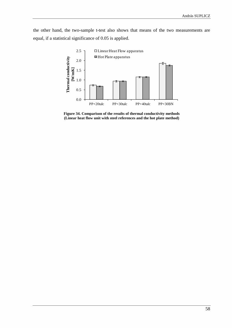
With the new instrument the thermal conductivity (TC) of four different samples were
measured and compared to the results of the hot plate method (Figure 34). The methods show
nearly the same results, the values are within the standard deviation of the measurements. On
András SUPLICZ
58
the other hand, the two-sample t-test also shows that means of the two measurements are
equal, if a statistical significance of 0.05 is applied.
0.0
0.5
1.0
1.5
2.0
2.5
PP+20talc PP+30talc PP+40talc PP+30BN
The
rma
l co
nduc
tivity
[W
/mK
]
Linear Heat Flow apparatus
Hot Plate apparatus
Figure 34. Comparison of the results of thermal conductivity methods (Linear heat flow unit with steel references and the hot plate method)
Development of injection moldable, thermally conductive polymer composites
59
5. Results and discussions
In this chapter the results of my researches are introduced and discussed.
5.1. Properties of thermally conductive polymer composites
A number of parameters have a significant influence on the thermal conductivity
coefficient of polymer compounds, including filler material, filler volume fraction, the
thermal conductivity of the filler and the polymer material etc. These parameters should be
investigated further to determine their exact effect on thermal conductivity.
5.1.1. The effect of the matrix
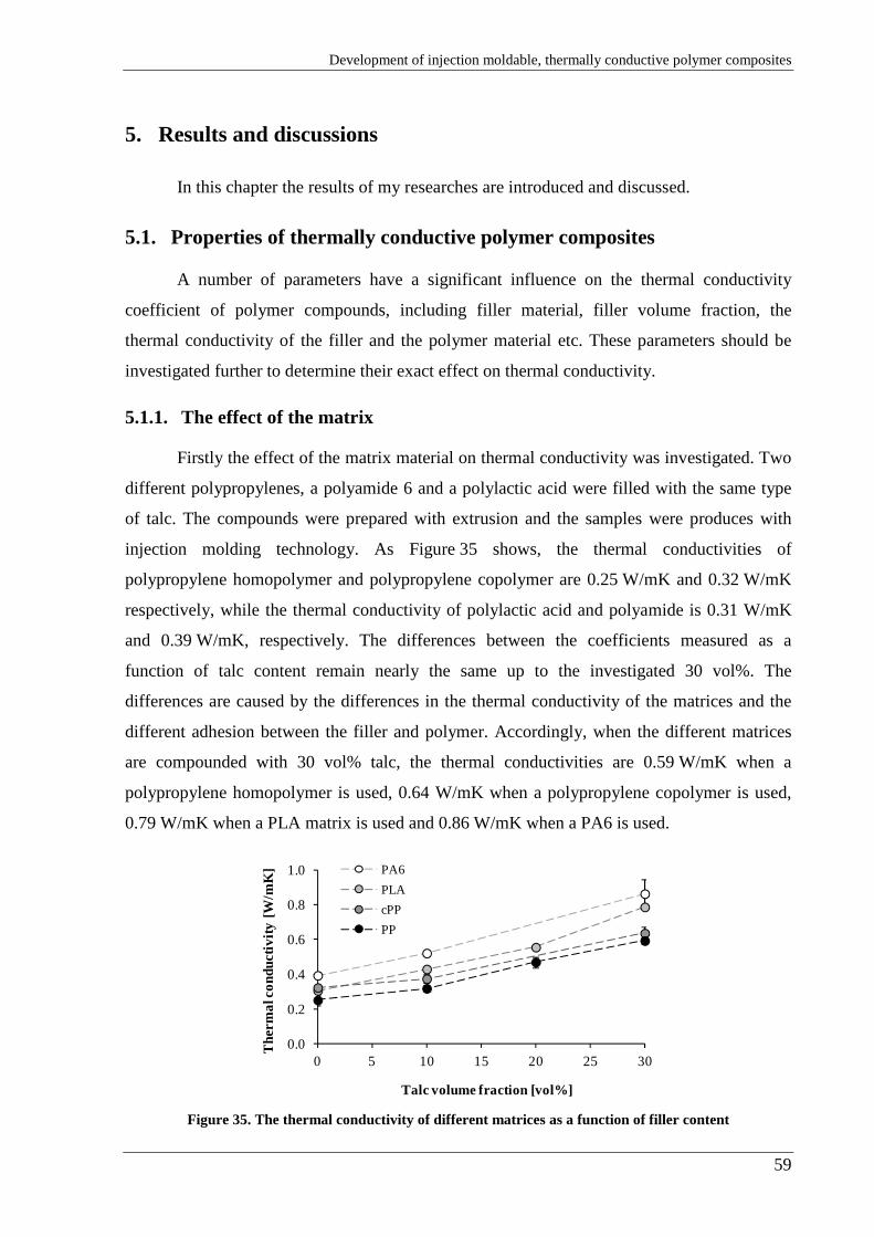
Firstly the effect of the matrix material on thermal conductivity was investigated. Two
different polypropylenes, a polyamide 6 and a polylactic acid were filled with the same type
of talc. The compounds were prepared with extrusion and the samples were produces with
injection molding technology. As Figure 35 shows, the thermal conductivities of
polypropylene homopolymer and polypropylene copolymer are 0.25 W/mK and 0.32 W/mK
respectively, while the thermal conductivity of polylactic acid and polyamide is 0.31 W/mK
and 0.39 W/mK, respectively. The differences between the coefficients measured as a
function of talc content remain nearly the same up to the investigated 30 vol%. The
differences are caused by the differences in the thermal conductivity of the matrices and the
different adhesion between the filler and polymer. Accordingly, when the different matrices
are compounded with 30 vol% talc, the thermal conductivities are 0.59 W/mK when a
polypropylene homopolymer is used, 0.64 W/mK when a polypropylene copolymer is used,
0.79 W/mK when a PLA matrix is used and 0.86 W/mK when a PA6 is used.
0.0
0.2
0.4
0.6
0.8
1.0
0 5 10 15 20 25 30
The
rma
l co
nduc
tivity
[W
/mK
]
Talc volume fraction [vol%]
PA6
PLA
cPP
PP
Figure 35. The thermal conductivity of different matrices as a function of filler content
András SUPLICZ
60
5.1.2. The effect of fillers
Secondly, the effect of filler material and filler content on the thermal conductivity of
the polymer matrix was investigated on injection molded samples. The matrix material was
polypropylene homopolymer and it was compounded with talc, boron nitride and titanium
dioxide. The filler content was varied between 0 and 30 vol%. Figure 36 shows the effect of
the different fillers on the thermal conductivity of the PP compounds. As it was expected,
thermal conductivity increases with filler content. Pure polypropylene has a thermal
conductivity of 0.25 W/mK. The thermal conductivity of the compounds rises slowly at low
filler volume fractions because the ceramic particles are dispersed evenly in the
polypropylene matrix and there is only little or no interaction between them. There are
significant differences between the thermal conductivities of the compounds at high filler
loading. The thermal conductivity coefficient of the composites filled with BN rises rapidly
but that of the samples filled with talc and titanium dioxide rises slowly. With 30 vol% filler,
the thermal conductivity coefficient of the compound is 0.6 W/mK with talc and almost
double that amount, 1.14 W/mK with boron nitride. The thermal conductivity of the
compound containing 30 vol% BN is more than four times higher than that of the pure PP.
0.0
0.2
0.4
0.6
0.8
1.0
1.2
1.4
0 10 20 30 40
The
rma
l co
nduc
tivity
[W
/mK
]
Filler content [vol%]
PP+BNPP+talcPP+TiO2
Figure 36. Thermal conductivity of PP homopolymer as a function of filler type and concentration
To characterize the changes in the mechanical properties of the compounds, quasistatic
and dynamic tests were performed. The results of the tensile test (as a quasistatic test) can be
seen in Figure 37 and Figure 38. In comparison to the unfilled polypropylene, particle filled
compounds have significantly smaller tensile strength. This might be due to the fact that there
is poor adhesion between the fillers and matrix. It can be improved with surface treatment of
the fillers.
Development of injection moldable, thermally conductive polymer composites
61
15
20
25
30
35
0 10 20 30 40
Ten
sile
str
eng
th [
MP
a]
Filler content [vol%]
PP+BN
PP+talc
PP+TiO2
Figure 37. Tensile strength of PP homopolymer-based composites as a function of filler type and concentration
The tensile modulus shows a reverse tendency (Figure 38). When fillers were added to
the polypropylene, the modulus increased. While the unfilled H145 F PP has a tensile
modulus of 2.1 GPa, the composites have a significantly higher (4-6 GPa) tensile modulus. It
means that the particles as a filler raise the stiffness of the compound.
0
2
4
6
8
0 10 20 30 40
Te
nsile
mo
dulu
s [G
Pa
]
Filler content [vol%]
PP+BNPP+talc
PP+TiO2
Figure 38. Tensile modulus of PP homopolymer-based composites as a function of filler type and concentration
As the typical loads of polymer parts have dynamic characteristics, Charpy tests were
performed. The results are shown in Figure 39. As can be seen, the unfilled polypropylene has
an impact strength of 72 kJ/m2. When 10 vol% talc is added to the matrix, a significant drop
can be observed, as the impact strength decreases to one-third of the impact strength of the
unfilled polypropylene. As filler content is increased, impact strength shows a decreasing
tendency. This drop is much more remarkable than the drop in tensile strength. At 30 vol%
filler content all the materials have the same impact strength, which is only 8 kJ/m2.
András SUPLICZ
62
0
10
20
30
40
50
60
70
80
90
0 10 20 30
Chr
py im
pact
str
eng
th,
a CU
[kJ/
m2 ]
Filler content [vol%]
PP+BN
PP+talc
PP+TiO2
Figure 39. Tensile modulus of PP homopolymer-based composites as a function of filler type and concentration
5.1.3. The effect of the processing method
Compression molding vs. injection molding
When the thermal conductivity of injection molded and compression molded samples
are compared, it can be seen that compression molded samples have higher thermal
conductivity (Figure 40). Using a polypropylene homopolymer matrix, and boron nitride and
talc as filler, the thermal conductivity of injection molded samples are 16-39% and 30-39%
lower than that of compression molded samples with 10-30 vol% filler concentration.
Furthermore, it can be seen that as filler concentration increases, the difference increases too.
There is also a difference in the thermal conduction of unfilled polypropylene. While the
injection molded sample has a conductivity coefficient of 0.25 W/mK, the compression
molded sample has a conductivity coefficient of 0.36 W/mK. This can be explained by the
difference in crystallinity and molecular chain orientation. When fillers are added to the
matrix, the differences in thermal conductivity increase as a function of filler content. Next to
the effect of the crystallinity and the molecular chain orientation of the matrix, the shell-core
effect of the fillers may have also a significant influence on thermal conductivity – there is an
insulating polymer layer on the surface of the injection molded samples. This effect is caused
by the segregation effect when the polymer fills the cavity. On the other hand, this difference
could also be caused by the orientation of the filler particles, as the thermal conductivity of
the particles has an anisotropic nature. Plate-like and fibrous particles show different thermal
properties in different directions. In compression molded samples the filler particles have
random orientations, while in the injection molded samples the orientation is determined by
the melt flow. This way injection molded parts have a lower thermal conductivity coefficient.
Development of injection moldable, thermally conductive polymer composites
63
0.0
0.2
0.4
0.6
0.8
1.0
1.2
0 10 20 30 40
The
rma
l co
nduc
tivity
[W
/mK
]
Talc volume fraction [vol%]
Compression moldedInjection molded
a)
0.0
0.5
1.0
1.5
2.0
0 10 20 30
The
rma
l co
nduc
tivity
[W
/mK
]
BN volume fraction [vol%]
Compression moldedInjection molded
b)
Figure 40. Thermal conductivity of talc (a) and boron nitride (b) filled composites prepared with compression molding and injection molding
This phenomenon was proved by SEM analysis. Figure 41 shows the SEM micrographs of the
fracture surface of shell and core layers of a 2 mm thick injection molded BN filled
polypropylene sample. In the shell layer highly oriented particles can be observed, which is
caused by the flow and high shear rate during the filling of the cavity. On the other hand,
unoriented particles can be observed in the core. The core layer is very thin, about
200-300 µm thick. One of the reasons may be the high thermal conductivity of the composite;
hence the frozen layer is thick and rapidly grows while the cavity is being filled.
a)
b)
Figure 41. SEM micrographs of an injection molded 10 vol% BN filled PP sample (a, shell layer; b, core layer)
Figure 42 shows the SEM images of the shell and core layers of a 2 mm thick compression
molded BN filled polypropylene sample. In contrast to the injection molded specimens, both
in the shell and in the core layer a random orientation of BN particles can be observed.
András SUPLICZ
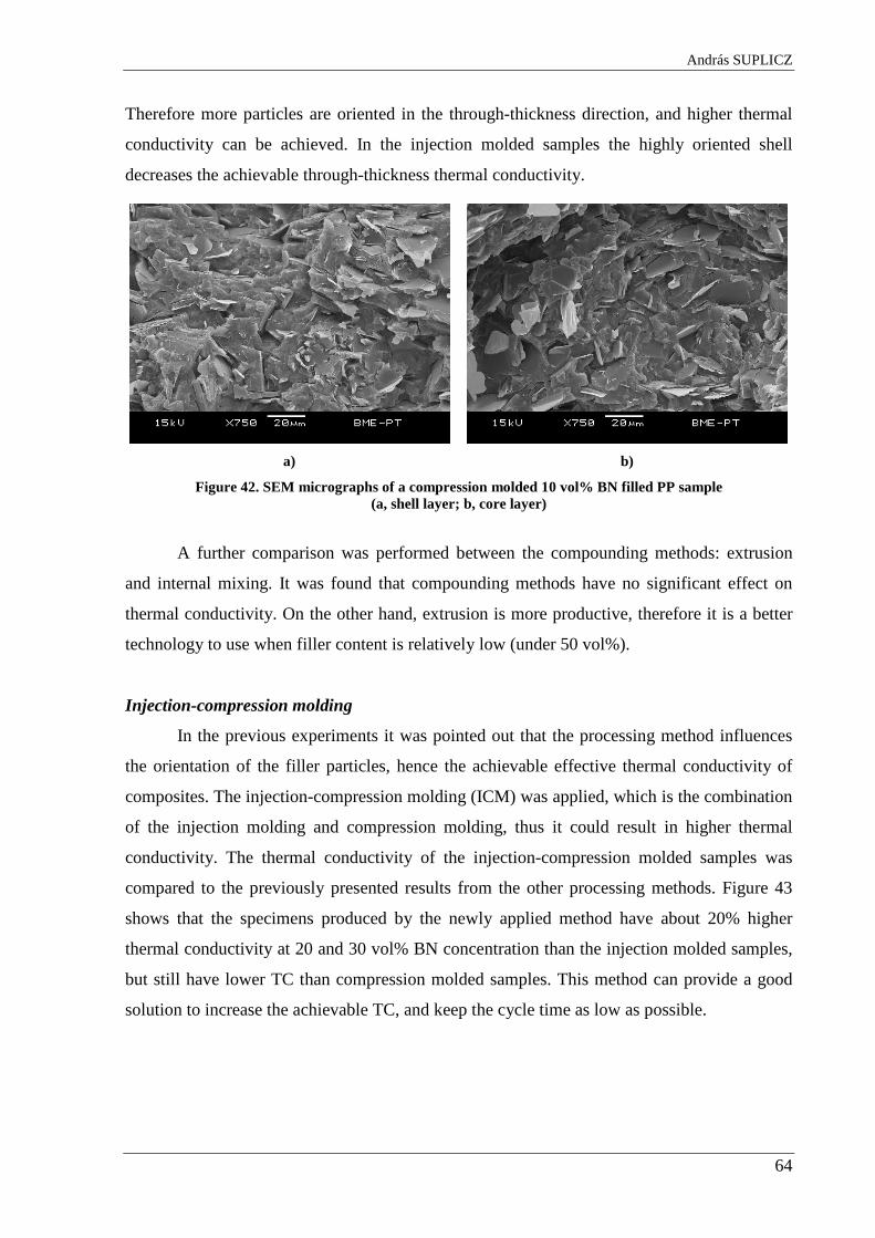
64
Therefore more particles are oriented in the through-thickness direction, and higher thermal
conductivity can be achieved. In the injection molded samples the highly oriented shell
decreases the achievable through-thickness thermal conductivity.
a)
b)
Figure 42. SEM micrographs of a compression molded 10 vol% BN filled PP sample (a, shell layer; b, core layer)
A further comparison was performed between the compounding methods: extrusion
and internal mixing. It was found that compounding methods have no significant effect on
thermal conductivity. On the other hand, extrusion is more productive, therefore it is a better
technology to use when filler content is relatively low (under 50 vol%).
Injection-compression molding
In the previous experiments it was pointed out that the processing method influences
the orientation of the filler particles, hence the achievable effective thermal conductivity of
composites. The injection-compression molding (ICM) was applied, which is the combination
of the injection molding and compression molding, thus it could result in higher thermal
conductivity. The thermal conductivity of the injection-compression molded samples was
compared to the previously presented results from the other processing methods. Figure 43
shows that the specimens produced by the newly applied method have about 20% higher
thermal conductivity at 20 and 30 vol% BN concentration than the injection molded samples,
but still have lower TC than compression molded samples. This method can provide a good
solution to increase the achievable TC, and keep the cycle time as low as possible.
Development of injection moldable, thermally conductive polymer composites
65
0.0
0.5
1.0
1.5
2.0
0 5 10 15 20 25 30
The
rma
l co
nduc
tivity
[W
/mK
]
BN volume fraction [vol%]
Compression molded
Injection-compression molded
Injection molded
Figure 43. Thermal conductivity of injection-compression molded PP/BN composites
The fracture surface of the ICM samples was analyzed with SEM. The rate of the shell
and core layers and the filler orientation was observed. In the shell the particles are
perpendicular to the direction of heat flow and in the core the particles are near parallel to the
heat flow. Because of the anisotropic nature of the BN particles, the higher the core/shell rate
in the sample, the higher its effective TC is. Figure 44 shows that the injection molded
samples have very thin core layer and the injection-compression molded ones have thicker
core, more than 600 µm.
a)
b)
Figure 44. SEM micrographs of injection molded (a) and injection-compression molded (b) 30 vol% BN filled PP samples
In the shell of ICM samples more unoriented sections can be observed which can
further increase the TC (Figure 45/a). Furthermore at the end of the flow path, which is filled
during the compression phase of ICM technology, the BN particles are oriented nearly
parallel to the through-thickness direction and only very thin shell layer can be observed
(Figure 45/b). Hence the particles have ideal orientation regarding to the heat dissipation, but
it results in different TC at the gate and at the end of the flow path.
András SUPLICZ
66
a)
b)
Figure 45. SEM micrographs of injection-compression molded 30 vol% BN filled PP samples: oriented and unoriented parts of shell layer (a) and filler orientation at the end of the flow path (b)
Segregation of fillers
To analyze the filler distribution along the flow path in injection molded samples, the
segregation of the talc and boron nitride was measured at different filler concentrations. As
the results show (Figure 46), actual filler concentration is in good agreement with nominal
concentration, and there is no significant segregation of talc and BN particles along the flow
path. It means that thermal conductivity and consequently the mechanical properties are
uniform along the flow length.
0
10
20
30
40
0 20 40 60 80
Ta
lc c
onc
entr
atio
n [v
ol%
]
Flow length [mm]
10 20 30Nominal concentration [vol%]:
a)
0
10
20
30
40
0 20 40 60 80
BN
co
nce
ntra
tion
[vo
l%]
Flow length [mm]
10 20 30Nominal concentration [vol%]:
b)
Figure 46. Talc (a) and boron nitride (b) concentration along the flow path in the polypropylene matrix
Static and dynamic mixers for injection molding
Different mixing elements (static and dynamic mixers) were also tested to show their
efficiency concerning homogenous mixing and thermal conductivity enhancement during
Development of injection moldable, thermally conductive polymer composites
67
injection molding. First of all a 30 vol% filler content masterbatch was prepared with a twin
screw extruder, then injection molded samples were made with 5, 10 and 20 vol% BN and
also with talc by dilution with polypropylene. Two 22 mm inner diameter Stamixco static
mixers were used with 5 (SM5) and 8 (SM8) mixing elements. The dynamic mixer was used
with two different parameter setups. The first run was performed at a low screw rotation
speed (15 1/min) and low back pressure (20 bar) (DM_1) and the second run at higher
rotation speed (35 1/min) and higher back pressure (60 bar) (DM_2). Reference samples were
also injection molded without mixing elements (SM0). Figure 47 shows the effect of different
mixers on the thermal conductivity of BN and talc filled polypropylene. It can be stated that
changing the number of static mixing elements causes no significant change in thermal
conductivity. On the other hand, the use of dynamic mixers results in only a minor
enhancement of thermal conductivity. The increase is less than 0.1 W/mK in the case of talc-
filled and less than 0.17 W/mK in the case of BN-filled composites. Hence it can be stated
that neither static nor dynamic mixers have a remarkable effect on thermal conductivity and
the homogeneous distribution of aggregates.
0.0
0.2
0.4
0.6
0 5 10 15 20
The
rma
l co
nduc
tivity
[W
/mK
]
Talc content [vol%]
0SM5SM8SMDM_1DM_2
a)
0.00
0.25
0.50
0.75
1.00
0 5 10 15 20
The
rma
l co
nduc
tivity
[W
/mK
]
BN content [vol%]
0SM5SM8SMDM_1DM_2
b)
Figure 47. Effect of different mixing elements on thermal conductivity of talc (a) and boron nitride (b) filled polypropylene composites (SM=static mixer; DM=dynamic mixer)
To further analyze the effect of mixing elements, mechanical tests were also
performed. As Figure 48 and Figure 49 show, there are also no significant differences in
mechanical properties between the composites prepared with a different number of static
mixing elements. On the other hand, dynamic mixing at a low screw rotation speed and low
back pressure caused a decrease in both tensile strength and tensile modulus. The difference is
minor compared to the other setups, but it can mean that the aggregates are not broken up and
András SUPLICZ
68
homogenized properly, which leads to impaired mechanical properties and an increase in
thermal conductivity.
20
25
30
35
0 5 10 15 20
Te
nsile
str
eng
th [
MP
a]
BN content [vol%]
0SM5SM8SMDM_1DM_2
a)
20
25
30
35
0 5 10 15 20
Ten
sile
str
eng
th [
MP
a]
Talc content [vol%]
0SM5SM8SMDM_1DM_2
b)
Figure 48. Tensile strength of BN (a) and talc (b) filled PP composites injection molded with different mixing elements (SM=static mixer; DM=dynamic mixer)
0
1
2
3
4
5
6
0 5 10 15 20
Ten
sile
mo
dulu
s [G
Pa
]
BN content [vol%]
0SM5SM8SMDM_1DM_2
a)
0
1
2
3
4
5
6
0 5 10 15 20
Ten
sile
mo
dulu
s [G
Pa
]
Talc content [vol%]
0SM5SM8SMDM_1DM_2
b)
Figure 49. Tensile modulus of BN (a) and talc (b) filled PP composites injection molded with different mixing elements (SM=static mixer; DM=dynamic mixer)
5.1.4. Surface modification
The most effective way to improve the thermal conductivity of composites is
increasing filler concentration. This method increases the apparent viscosity of the material
and it could cause problems during processing. Surface treatment could be an alternative
method to improve the thermal conductivity of the composites at given filler content. The
surface of BN is very inert and it leads to poor interfacial adhesion between the particles and
the polymer. It is well-known that a coupling agent can improve the phase interfacial bonding
strength between filler and matrix, which enhances thermal conductivity as well as
Development of injection moldable, thermally conductive polymer composites
69
mechanical properties. Thus a good contact between the phases is critical to the efficiency of
heat flow. Thermal conductivity is very sensitive to interface defects because the thermal
contact resistance between the filler and matrix leads to a phonon-scattering effect.
Three different surface treatment methods were applied on boron nitride powder based
on the works of Xu and Chung [134], Zhou et al. [135] and Kim et al. [136]. The three
methods were the followings:
1st method (M1): a silane/distilled water solution was prepared with 2.4 m% silane
concentration with reference to the amount of BN. First BN was added to the solution and
stirred at room temperature for 30 minutes, then stirred at 80°C for 1 hour. The mixture was
dried out at 90°C in a drying chamber for 4 hours.
2nd method (M2): 2.4 m% silane (with reference to the amount of BN) was added to
the 95/5 m% distilled water/ethanol solution adjusted to pH 4.5 with diluted hydrochloric
acid. Boron nitride powder was added to the solution and stirred at room temperature for
30 minutes, then stirred at 80°C for 1 hour. The mixture was dried out at 90°C in a drying
chamber for 4 hours.
3rd method (M3): boron nitride powder was treated with a 5M NaOH (20 g /100 ml)
solution for 5 hours at 80°C, and then the powder was rinsed and washed three times with
distilled water to reach the neutral pH. Next the silane treatment was performed according to
the 2nd method.
BN particles have a plate-like shape. Its basal plane is molecularly smooth and has no
surface functional groups available for chemical bonding. On the other hand, its edge planes
have hydroxyl and amino functional groups. These functional groups allow the BN to
chemically bond with other molecules. This is the reason why in the third method it was
treated with a NaOH solution, to attach more hydroxide ions onto the surfaces.
PP based composites were prepared from untreated and the surface treated BN powder
with an internal mixer at 30 vol% filler content. The samples were produced with
compression molding. For reference samples unfilled PP was used. The thermal conductivity
of the composites (Figure 50) was determined with the hot plate apparatus. PP has a thermal
conductivity of 0.36 W/mK and the thermal conductivity of PP filled with untreated BN is
1.92 W/mK, which is a 433% increase. The results show that the best method of the three is
the third surface treatment method; with it a thermal conductivity of more than 2.5 W/mK can
be achieved. It presents close to 700% increase compared to neat PP.
András SUPLICZ
70
0.0
0.5
1.0
1.5
2.0
2.5
3.0
neat PP UT M1 M2 M3
The
rma
l co
nduc
tivity
[W
/mK
]
Figure 50. Thermal conductivity of the 30 vol% BN filled compounds with different surface treatments (UT=untreated; M1–M3=1st method–3rd method)
The mechanical properties of the composites were also analyzed. According to the
results (Figure 51), it can be stated that the filled polypropylene has higher stiffness than the
unfilled PP. All surface treatment methods increased mechanical properties, both tensile
strength and modulus. The best mechanical properties can be obtained with the 1st and the 2nd
method. It also proves that the silane coupling agent increased the interfacial adhesion
between the PP and the BN.
0
5
10
15
20
25
30
35
neat PP UT M1 M2 M3
Ten
sile
str
eng
th [
MP
a]
a)
0
1
2
3
4
5
neat PP UT M1 M2 M3
Ten
sile
mo
dulu
s [G
Pa
]
b)
Figure 51. Tensile strength (a) and tensile modulus (b) of the 30 vol% BN filled compounds with different surface treatments
(UT=untreated; M1–M3=1st method–3rd method)
Table 7 lists the DSC results. The calculated crystallinity shows that silane surface
treatment does not modify the crystallinity of the composites. The untreated PP/BN composite
has a crystal fraction of 64.7% and after surface modification, the matrices have a 63-64%
crystal fraction. When these results are compared to the crystallinity of neat PP, a 5%
increment can be observed in all cases, which shows the nucleating efficiency of BN.
Development of injection moldable, thermally conductive polymer composites
71
Furthermore, a shift can be observed in melting and crystallization temperature. Melting
temperature decreased by 4°C due to the increased thermal conductivity. Crystallization
temperature increased about by 10°C, which also proves the nucleating efficiency of the filler.
These results are also presented in the Appendix (Chapter 9, Figure 89 and Figure 90).
Material Melting
temperature Crystallization temperature
Enthalpy of fusion
Crystallinity
[°C] [°C] [J/g] [%]
PP 162.95 123.56 96.49 58.48
PP+BN (UT) 159.12 133.36 53.38 64.70
PP+BN (M1) 158.37 134.01 52.03 63.07
PP+BN (M2) 159.44 138.30 52.16 63.22
PP+BN (M3) 156.30 130.72 52.72 63.90
Table 7. DSC measurement results of the PP/BN compounds (UT=untreated; M1–M3=1st method–3rd method)
5.1.5. The hybridization of fillers
To show the hybrid effect between boron nitride and talc, further measurements were
performed. In this case the thermal conductivity of three compression molded specimens was
measured. Table 8 contains the notation of the compounds and specimens. The specimens had
a thermal interface material between them, which reduced thermal resistance (Figure 52).
First the thermal conductivity of hybrid materials were determined (H1 and H2), using three
specimens joined together in each measurement. Secondly, the thermal conductivity of
materials with a single filler was determined (compounds A and B). Thirdly, the conductivity
of the specimens joined together (Figure 52) was determined. A system made up of specimens
filled with a single filler was also tested, first with specimen arrangement AAB then with
ABB. Total filler content was 30 vol% in each case and the boron nitride and talc content was
the same as in the case of the hybrid material, but only specimens with a single filler were
used for the measurement of thermal conductivity.
Sign Compound A H145 F PP + 30 vol% talc B H145 F PP + 30 vol% BN H1 H145 F PP + 20 vol% talc + 10 vol% BN (hybrid) H2 H145 F PP + 10 vol% talc + 20 vol% BN (hybrid)
Table 8. Notation of the single and hybrid composites
András SUPLICZ
72
Figure 52. Arrangements for thermal conductivity measurements (a and b are compounds with 30 vol% single filler; c is a compound with 30 vol% hybrid filler)
As Figure 53 shows, in the case of specimens containing a single filler, a linear
relationship can be observed between the thermal conductivity of boron nitride and talc filled
specimens. Thus thermal conductivity can be easily calculated as a function of filler content.
If talc and boron nitride are hybridized, a higher thermal conductivity can be achieved and the
relationship between the fillers becomes nonlinear. As was mentioned, this positive synergetic
effect can be explained with the different particle size of BN and talc and the fragmentation of
talc particles. In the compound the talc particles formed the main thermally conductive path in
the compound, while the smaller BN particles established more contact between the larger
particles to obtain higher thermal conductivity.
Figure 53. Comparison of the effect of single and hybrid BN/Talc fillers on thermal conductivity of compression molded samples
Next, the thermal conductivity of the injection molded and the compression molded
samples were compared to each other, which showed the effect of the sample preparation
methods on hybrid filled composite materials. The same compound was used for both sample
preparation methods, thus filler content was the same. Before compression molding the
samples, the granules were milled to avoid air traps during the process. The measurement
Development of injection moldable, thermally conductive polymer composites
73
results can be seen in Figure 54. At each measurement point the thermal conductivity of the
compression molded samples was about 60% higher than that of the injection molded ones. It
proves that the skin-core effect has great influence on thermal conductivity. The skin layer has
lower filler content, thus it behaves as an isolating layer, which decreases heat transfer.
Figure 54. Comparison of the effect of molding process on BN/Talc hybrid filled H145 F PP
To characterize the changes in mechanical properties of the compounds, quasistatic
and dynamic tests were performed. The results of the tensile test (as a quasistatic test) can be
seen in Figure 55 and Figure 56. Compared to unfilled polypropylene, particle-filled
compounds have significantly lower tensile strength. The tensile strength of unfilled PP
(31.9 MPa) decreased by 6-10 MPa when 30 vol% filler was added.
20
22
24
26
PP: 70BN: 0talc: 30
PP: 70BN: 10talc: 20
PP: 70BN: 20talc: 10
PP: 70BN: 30talc: 0
Ten
sile
str
eng
th [
MP
a]
Filler composition [vol%]
Figure 55. The tensile strength of the compounds
The tensile modulus shows a reverse tendency (Figure 56). When fillers are added to
the polypropylene, the modulus increased significantly. While the unfilled PP has a tensile
modulus of 2.1 GPa, the PP/10 vol% BN 20 vol% talc compound has a tensile modulus three
times higher (6 GPa). It means that the particles as reinforcement increase the stiffness of the
András SUPLICZ
74
compound. It was also found that BN has a better reinforcing effect than talc. Filling 30 vol%
talc into the matrix increased the modulus by 2.8 GPa. When the same amount of BN was
used, the modulus increased by 3.7 GPa. With hybrid fillers a higher modulus can be
achieved. It means that a synergetic effect exists between talc and BN.
2
4
6
8
PP: 70BN: 0talc: 30
PP: 70BN: 10talc: 20
PP: 70BN: 20talc: 10
PP: 70BN: 30talc: 0
Te
nsile
mo
dulu
s [G
Pa
]
Filler composition [vol%]
Figure 56. Tensile modulus of the compounds
As the typical loads of polymer parts have dynamic characteristics, Charpy impact
tests were also performed. The results of the measurements can be seen in Figure 57. The
unfilled polypropylene has an impact strength of 72 kJ/m2. When 30 vol% talc is added to the
matrix, a significant drop can be observed, as impact strength lowered to one-tenth of that of
unfilled polypropylene. This drop is far more remarkable than the drop in tensile strength. The
most brittle of the compounds is polypropylene containing 20 vol% BN and 10 vol% talc. Its
impact strength is only 3.6 kJ/m2. The results show that in contrast to tensile modulus, hybrid
materials have a negative synergetic behavior concerning impact strength.
0
2
4
6
8
10
PP: 70BN: 0
talc: 30
PP: 70BN: 10talc: 20
PP: 70BN: 20talc: 10
PP: 70BN: 30talc: 0
Cha
rpy
impa
ct s
tre
ngth
[k
J/m
2 ]
Filler composition [vol%]
Figure 57. Impact strength of single filled and hybrid materials
Development of injection moldable, thermally conductive polymer composites
75
With the Melt Volume Rate (MVR) measurement the compounds can be characterized
regarding the processability. The MVR values of the single and hybrid filled compounds is
shown on Figure 58. The melt volume rate of the unfilled polypropylene is 44 cm3/10 min.
Filling 30 vol% talc into the matrix, the MVR decrease to 11.8 cm3/10 min and at the case of
30 vol% boron-nitride this value is only 2.5 cm3/10 min. Boron-nitride and talc as hybrid
filler has a negative hybrid effect to the viscosity. The compound, containing 20 vol% BN and
10 vol% talc has lower MVR value (1.65 cm3/10 min) than that of the 30 vol% boron-nitride
filled PP.
0
5
10
15
PP: 70BN: 0talc: 30
PP: 70BN: 10talc: 20
PP: 70BN: 20talc: 10
PP: 70BN: 30talc: 0
MV
R [
cm3 /
10
min
]
Filler composition [vol%]
Figure 58. Melt volume rate of single filled and hybrid materials
5.2. Crystallinity of conductive polymer composites
Many papers have investigated the influence of filler fraction on thermal conductivity
and mechanical properties, but few of them have examined crystallinity, thermal parameters,
cooling behavior and their relationship. One of the most important physical parameters of
semi-crystalline polymers is their degree of crystallinity, as it determines their mechanical
properties. The modulus of elasticity, yield stress and impact resistance increase gradually
with crystallinity. Crystallinity and crystalline morphology are critical parameters during
injection molding because they are strongly influenced by processing conditions, including
molding temperature, cooling rate, holding time and temperature. There is a correlation
between cooling rate and crystallinity. The degree of crystallinity is proportional to the
cooling rate, and it can be determined by DSC measurements. Furthermore, the fillers added
to increase thermal conductivity can work as an effective nucleating agent. Thus they can
increase the number of crystal nuclei. In this chapter the effects of different ceramic fillers on
the cooling rate and thermal properties of polypropylene-based compounds are examined.
András SUPLICZ
76
5.2.1. Method of calculation
The temperature distribution in the specimen can be described with the heat diffusion
equation (Equation (38)) [10]. This differential equation was solved numerically with a finite
difference equation (explicit difference method) (Equation (39)). This numerical method
describes the cooling process in the substance using a one-dimension model without an inner
heat source [137].
λαq
Tt
T &+∇=
∂∂⋅ 21
. (38)
2
),(2),(),(),(),(
x
txTtxxTtxxT
t
txTttxT
∆−∆−+∆+⋅=
∆−∆+ α , (39)
where T is the temperature, x and t indicate the position and time, ∆x and ∆t are the distance
and time step in the calculation, and α is the thermal diffusivity. Thermal diffusivity was
calculated as the proportion of thermal conductivity and the product of density and specific
heat capacity (Equation (40)). Using temperature-dependent values in the equations, more
accurate results can be achieved.
)(
)()(
Tc
TT
p⋅=
ρλα , (40)
where ρ is density, cp is specific heat capacity and λ is thermal conductivity.
In an actual process the polymer shrinks and warps during cooling, therefore thermal
contact resistance (Rs) varies during the cycle. Several studies have examined thermal contact
resistance between the polymer and the metal surface, in which the mean value of resistance
is 5·10-4 m2K/W [138, 139]. Contact resistance induces a temperature difference between the
polymer (Tps) and the surface of the mold (Tms). Equation (41) gives the temperature field
which is the input data of the explicit difference method.
mssps TtqRtT +⋅= )()( . (41)
The heat flux (q) was calculated from the temperature drop (∆T) in the substance between two
discrete points (∆x) (Equation (42)), according to Fourier’s law. This heat also flows through
the air gap between the surface of the mold and the polymer.
x
Ttq
∆∆⋅= λ)( . (42)
The cooling rate of the sample was calculated from the temperature field, which was obtained
from the explicit difference method. The derivation of the time-temperature curves at discrete
distances from the surface gives the cooling rate (vcool) as a function of time and distance
(Equation (43)).
Development of injection moldable, thermally conductive polymer composites
77
t
txTtxvcool ∂
∂= ),(),( . (43)
The cooling time required to reach the ejection temperature was determined with three
different methods: simulation; the explicit difference method and an empirical formula
(Equation (44)) [140]. The simulations were performed with the Moldflow injection molding
simulation software.
−−⋅⋅
⋅=
moe
momecool TT
TTst
παπ4
ln2
, (44)
where s is the thickness of the sample, Tme is the melt temperature, Tmo is the temperature of
the mold and Te is the ejection temperature.
5.2.2. Cooling rate in the sample
The three stages of specific heat measurement (heat-cool-heat) are plotted in Table 9.
Only unfilled PP shows a significant difference between the first and the second heating,
which is about 500 J/kgK. In the case of the filled materials there is no considerable
difference between the two measurements. In the neat PP the first heating phase refers to the
injection molding process, and the second heating to the behavior caused by controlled
cooling. In the filled PP this effect is not significant as there are no changes in the fillers at
this low temperature range, therefore the high filler content leads the process. On the other
hand, there are significant differences between the values measured in the heating and the
cooling phase. The specific heat measured during the cooling phase has to be used for
calculations, as Equation (39) describes a cooling process.
Material Specific heat [J/kgK] (25-225°C)
1st heating cooling 2nd heating H145 F 1460-1930 2030-3140 1950-2630
H145 F + 30 vol% talc 1390-2030 1550-2000 1440-1920 H145 F + 30 vol% BN 1390-2030 1500-2150 1380-2060 H145 F + 30 vol% TiO2 1960-2045 1660-2350 1780-1960
Table 9. Specific heat of the compounds
The cooling gradients were determined as a function of the time and positions across
the thickness using the explicit difference method. In accordance with the injection molding
tests, a melt temperature of 200°C and a mold temperature of 40°C were used in the
calculations. Specific heat and, as a result, calculated heat diffusivity varied as a function of
temperature. The temperature was uniform throughout the whole specimen at the initial
András SUPLICZ
78
calculation step, then it started to cool down to 40°C. The cooling gradients (Figure 59) show
that unfilled PP has the lowest cooling rate. When 30 vol% of filler is used, cooling time can
be shortened significantly. The maximum ejection temperature of polypropylene is about 100-
110°C. It means that if the temperature is lowered below this value, the polymeric parts are
hard enough to be removed from the mold without any damage [141]. With 30 vol% of TiO2
the cooling time to reach ejection temperature decreased by 35%, with talc it decreased by
50% and in the case of BN by more than 70%.
The time to reach ejection temperature in the cross-section is shown in Figure 60.
From the cooling gradients the cooling rates can be calculated. Figure 61 shows the average
cooling rate of the material between the injection temperature (200°C) and the ejection
temperature (100°C) as a function of position across the thickness. On the surface a very high
cooling rate can be observed, but it decreases rapidly towards the center. In the middle of the
PP sample the average cooling rate is 22.6°C/s. With 30 vol% of talc the cooling rate is
45.8°C/s, with TiO2 it is 57.1°C/s and with BN it increases to 75°C/s. These significant
differences in the cooling rates can be explained with the differences in thermal conductivity
(Figure 62). Moreover, there is a strong linear correlation between the cooling rate and
Table 10. Melting and crystallization characteristics of the compounds
Development of injection moldable, thermally conductive polymer composites
81
In the DSC measurements, the thermal history of the materials was erased during the
first heating, then the crystals were created and melted under controlled circumstances with a
slow cooling and heating rate. This method is widely used when a small amount of filler is
added to the polymer matrix. This way the effect of the fillers on crystallinity can be
compared. On the other hand, in a real process such as injection molding, the cooling rate is
more than 15°C/s, thus the polymers have less time for crystallization. The higher the cooling
rate, the lower crystallinity will be. Process-induced crystallinity can be obtained from the
first heating scan of DSC measurements.
The results of the crystallinity measurements are shown in Figure 65. It can be seen
that the degree of crystallinity increased with the addition of fillers when the heating and
cooling rate was 10°C/min (the second heating and the first cooling). Titanium dioxide
increased the crystallinity of PP from 63% to 71%. BN or talc only increased it to 65-66%.
Among the three filler types, the best nucleating agent is the BN, because the PP/BN
composite shows the highest crystallization temperature. Injection molding-induced
crystallinity was determined from the first heating phase. It is noticeable that crystallinity is 5-
15% lower than after recrystallization. With 30 vol% boron nitride crystallinity is only 64.2%,
which is lower than in the case of unfilled polypropylene (68.1%). This drop can be explained
by the higher thermal conductivity of the composite. While the unfilled polypropylene cooled
slowly in the mold after injection, the 30 vol% boron nitride filler increased thermal
conductivity and also the cooling rate. Due to the higher cooling rate, lower crystallinity can
be obtained. It means that the nucleating effect of the boron nitride was not enough to
compensate for the effect of thermal conductivity.
40
45
50
55
60
65
70
75
PP PP+talc PP+BN PP+TiO2
Cry
sta
llini
ty [%
]
Crystallinity in the first heating
Crystallinity in the second heating
Figure 65. Crystallinity of the compounds in the first and second heating phase
The crystallinity of talc and BN filled compounds were investigated as a function of
filler content and the thermal conductivity of the composite. Up to 30 vol% talc
András SUPLICZ
82
(λ=0.58 W/mK) crystallinity increased monotonously, which shows a good nucleating agent
behavior. On the other hand, when boron nitride is added to the PP matrix, first crystallinity
increases, then above a threshold it decreases. This limit value is 10 vol%, where the thermal
conductivity of the compound is 0.55 W/mK. Above 10 vol% BN fraction, the high thermal
conductivity results in faster cooling during injection molding, thus crystallinity decreases
(Figure 66).
50
55
60
65
70
0.2 0.4 0.6 0.8 1.0 1.2
Cry
sta
llini
ty [%
]
Thermal conductivity [W/mK]
PP+talc 2nd heating
PP+BN 2nd heating
PP+talc 1st heating
PP+BN 1st heating
filler content
Figure 66. The crystallinity of PP compounds as a function of talc (0, 10, 20 and 30 vol%) and BN (0, 4.4, 12.1, 20 and 30 vol%) content
To prove this phenomenon, further investigation was performed with polylactic acid
(PLA) matrix composites. PLA has low crystallinity even at a very low cooling rate (without
using nucleating agents). During processing, when the cooling rate is much higher, the
material can remain amorphous. Nucleating agents, like talc or boron nitride can enhance the
crystalline ratio of PLA significantly, and the effect of the thermal conductivity of the
compounds can be analyzed and compared.
According to the measurements on the injection molded samples, the unfilled PLA has
a thermal conductivity of 0.31 W/mK (Figure 67).
0.0
0.5
1.0
1.5
0 5 10 15 20 25 30
The
rma
l co
nduc
tivity
[W
/mK
]
Filler content [vol%]
PLA+talc
PLA+BN
Figure 67. The thermal conductivity of talc and BN filled injection molded PLA samples
Development of injection moldable, thermally conductive polymer composites
83
When a filler was added to the matrix, TC changed significantly. With 30 vol% BN, thermal
conductivity increased by 365% (1.44 W/mK) and with 30 vol% talc it increased by 155%
(0.79 W/mK).
As Figure 68 shows talc-filled PLA has a well-determined crystallization peak. The
curves indicate that talc is a good nucleating agent because there is no cold crystallization
during the second heating phase. With BN as filler the crystallization peak is much lower and
in the second heating phase cold crystallization can be observed. This phenomenon can have
two main reasons. First, BN is not as good a nucleating agent as talc; second, its thermal
conductivity is much higher than that of talc, which increases the cooling rate inside the
sample during the measurement.
0 50 100 150 200
Hea
t flo
w (e
xo u
p)
Temperature [°C]
PLA+20 vol% talc
PLA+20 vol% BN
a)
0 50 100 150 200
Hea
t flo
w (e
xo u
p)
Temperature [°C]
PLA+20 vol% talc
PLA+20 vol% BN
b)
Figure 68. DSC measurements of 20 vol% talc and BN filled compounds at a heating/cooling rate of 10°C/min (a, 1st cooling; b, 1st heating)
The crystallinity of talc and BN filled PLA was investigated as a function of filler
content (Figure 69).
0
10
20
30
40
50
0.2 0.4 0.6 0.8 1.0 1.2 1.4 1.6
Cry
sta
llini
ty [%
]
Thermal conductivity [W/mK]
PLA+talc 2nd heating
PLA+BN 2nd heating
PLA+talc 1st heating
PLA+BN 1st heating
filler content
Figure 69. The crystallinity of PLA compounds as a function of talc (0, 10, 20 and 30 vol%) and BN (0, 10, 20, and 30 vol%) content
András SUPLICZ
84
Up to 30 vol% talc (λ=0.79 W/mK) crystallinity increased monotonously, which shows a
good nucleating agent behavior. On the other hand, when boron nitride is added to PLA, first
the crystalline ratio increases then after a threshold it decreases. This limit value is 20 vol%,
where the thermal conductivity of the compound is 0.82 W/mK. Above 20 vol% BN fraction,
the high thermal conductivity results in faster cooling during injection molding, thus
crystallinity decreases. This phenomenon was also detected previously in the case of the PP
matrix.
5.2.4. Isothermal crystallization
The isothermal crystallization of an unfilled polypropylene homopolymer and its
compounds with boron nitride was analyzed. The isothermal crystallization kinetics of a
material at a constant temperature can be described by evaluating its degree of crystalline
conversion as a function of time. Relative crystallinity at different crystallization times (X(t))
can be calculated with Equation 45 [142]:
∫
∫∞
∞
==
0
0
)/(
)/(
)(
dtdtdH
dtdtdH
Q
QtX
t
t , (45)
where Qt is the heat generated at time t, Q∞ is the heat generated at infinite time, and dH/dt is
the rate of heat production. In order to understand the evolution of crystallinity during
isothermal crystallization, the Avrami model was applied to analyze isothermal crystallization
kinetics (Equation 46):
ntKetX ⋅−−= 1)( , (46)
where n is the Avrami exponents. The value of n depends on the mechanism of nucleation and
the form of crystal growth, while K is a rate constant dedicated to nucleation and growth.
Exponent n consists of two terms, one from nucleation (0 or 1) and one from crystallization
(1, 2 or 3) (Table 11). If the number of nuclei is constant in time (athermal nucleation), n
gives the dimension of crystal growth directly. On the other hand, if the number of nuclei
increases in time during crystallization (thermal nucleation), n is equal to the dimension of
growth+1 [143].
Development of injection moldable, thermally conductive polymer composites
85
n Crystal geometry Nucleation type 3+1 sphere thermal 3+0 sphere athermal 2+1 disc thermal 2+0 disc athermal 1+1 rod thermal 1+0 rod athermal
Table 11. Definition of the Avrami exponent n [142, 144]
Using the logarithmic form of the Avrami equation (Equation 47.) and fitting the
experimental data, the values of n and K can be determined from the slope and intercept of the
plots of log[-ln(1-X(t))] versus log t:
tnKtX loglog))](1ln(log[ ⋅+=−− . (47)
The isothermal crystallization in the melt of the PP and its compounds was analyzed at
four different temperatures (Tc: 130, 135, 140 and 145°C) with a DSC apparatus. The samples
were heated up to 200°C at 25°C/min and kept at a constant temperature for 5 minutes to
eliminate its thermal history. Then it was rapidly cooled down (50°C/min) to the previously
determined temperatures and maintained there for 40 minutes. The exothermic curves of heat
flow were recorded as a function of time. Figure 70 shows the isotherm crystallization curves
of the H145F PP/5 vol% BN compound at four different temperatures. Further results are
presented in the Appendix (Chapter 9, Figure 91).
0
2
4
6
8
10
12
14
16
0 5 10 15
He
at f
low
[mW
] (E
xo U
p)
Time [min]
130°C
135°C
140°C
145°C
Figure 70. Isotherm crystallization of polypropylene homopolymer + 5 vol% BN at different crystallization temperature
It was observed that when the crystallization temperature is increased, the exothermal
peak becomes broader, which implies that the crystallization rate is reduced. Thus, the
induction time of the exotherm increases. Furthermore the position of the crystallization peaks
of boron nitride filled PP appeared earlier than that of unfilled PP. The relative amount of
crystallization of PP/5 vol% BN compound has been plotted in Figure 71 for different
András SUPLICZ
86
crystallization temperatures. It was calculated from the exotherms of the DSC measurements.
Further results are presented in the Appendix (Chapter 9, Figure 92).
0
20
40
60
80
100
0 5 10 15 20
Re
lativ
e c
ryst
alli
nity
[%]
Time [min]
130°C
135°C
140°C
145°C
Figure 71. Relative crystallinity of the polypropylene homopolymer + 5 vol% BN as a function of time at different temperatures
Half-time of crystallization (t0.5) is defined as the time at which the extent of
crystallization is 50%. It can be read conveniently from the relative crystallinity–time curves,
and is also regarded as a very important crystallization kinetic parameter. Usually t0.5 is
employed to characterize the rate of crystallization directly. The greater the value of t0.5 is, the
lower the rate of crystallization is. As Figure 72 shows, the crystallization rate can be
increased significantly by adding boron nitride to the PP matrix.
0
5
10
15
130 135 140 145
Ha
lf ti
me
of c
ryst
alli
zatio
n [m
in]
Crystallization temperature [°C]
PP
PP+5BN
PP+10BN
PP+20BN
PP+30BN
Figure 72. Half time of crystallization of the polypropylene homopolymer and its compounds as a function of crystallization temperature
For example at 140°C, crystallization is 5 times faster when 5 vol% BN is added to the PP,
and 30 times faster when 30 vol% BN is filled into the matrix. It shows that BN is an effective
nucleating agent.
Development of injection moldable, thermally conductive polymer composites
87
Finally, the Avrami constants were determined by plotting the experimental data in the
log[-ln(1-X(t))] versus log t diagram (Figure 73). (Further results are presented in the
Appendix, in Chapter 9 on Figure 93.) n and K can be determined from its equation by data
fitting. The constants and half time of crystallization values are plotted in Table 12.
y = 1.81x + 0.72
y = 1.94x + 0.01
y = 2.06x - 0.94
y = 2.18x - 1.99-2.0
-1.5
-1.0
-0.5
0.0
0.5
1.0
-1 0 1
log
[-ln(
1-X
)]
log(t)
130°C:
135°C:
140°C:
145°C:
Figure 73. Avrami plots of log[-ln(1-X(t))] versus log t for isothermal crystallization of the polypropylene homopolymer + 5 vol% BN at different crystallization temperatures
Table 12. Avrami constants (n and k) and the half time of the crystallization of the compounds
As Table 12 shows, exponent n of the unfilled PP is about 3, which indicates that the
growth of crystals in the melt is probably three-dimensional (spherulite), and the nucleation
process is athermal. According to the literature, in the presence of a heterogeneous nucleating
agent the crystallization is supposed to be athermal [145]. Accordingly, when the boron
nitride fraction is increased, the crystals will be disc-shaped. On the other hand, when the
crystallization temperature is increased, exponent n also increases, thus crystallization and
nucleation kinetic change with temperature.
András SUPLICZ
88
5.3. Improving processability of conductive polymer composites
The processability of highly filled polymeric materials is a key issue in research and in
the industry as well. The fillers drastically decrease the flowability of the melt, thus energy
consumption increases and throughput decreases. In order to improve the processability of the
filled polypropylene, cyclic butylene terephthalate oligomer (CBT) was added to the matrix.
The effect of CBT 100 concentration
First, the effect of CBT content on the properties of the PP matrix was analyzed. 0.5,
1, 3 and 5 vol% of CBT 100 was blended with PP in a twin screw extruder then flat
80x80x2 mm samples were injection molded. As Figure 74 shows, the tensile strength of neat
PP is about 30 MPa, and as CBT content is increased, there is only a minor effect, but the
results are within the standard deviation of measurements. The same effect can be observed in
the tensile modulus (Figure 75). When CBT content is increased, the results are also within
the standard deviation of measurements. It can be established that the CBT 100 additive has
only a minimal effect on tensile strength and tensile modulus.
25
27
29
31
33
35
0.0 0.5 1.0 3.0 5.0
Ten
sile
str
eng
th [
MP
a]
CBT 100 content [vol%]
Figure 74. Tensile strength of PP/CBT compounds as a function of CBT content
1500
1750
2000
2250
2500
0.0 0.5 1.0 3.0 5.0
Ten
sile
mo
dulu
s [M
Pa
]
CBT 100 content [vol%]
Figure 75.Tensile modulus of PP/CBT blend as a function of CBT content
Development of injection moldable, thermally conductive polymer composites
89
Thermal conductivity was also measured. The tests were performed with a hot plate
apparatus at 55°C. The result shows that the CBT additive does not modify the thermal
conductivity of the polypropylene matrix (Figure 76). Further measurements need to be
carried out to study the effect of CBT on fillers. As CBT 100 is a good dispersion agent and
also a good wetting agent, it can develop better contact between the filler and the polymer,
thus reducing contact resistance and enhancing conductivity.
0.0
0.1
0.2
0.3
0.4
0.5
The
rma
l co
nduc
tivity
[W
/mK
]
Figure 76. Thermal conductivity of PP/CBT 100 blend
The results of the melt volume rate measurement show that when the CBT fraction in
the blend is increased, MVR also increases (Figure 77). In the 0-5 vol% range the relationship
between the CBT fraction and the MVR value is non-linear. By adding 5 vol% CBT 100 to
the PP, MVR increased by more than 100%. Up to 3 vol% CBT only a minor change can be
observed in the melt flow rate but above 3 vol% it changes drastically.
0
20
40
60
80
100
0 1 2 3 4 5
MV
R (
23
0°C
, 2
.16
kg
) [c
m3 /
10
min
]
CBT100 concentration [vol%]
Figure 77. Melt Volume Rate of the PP/CBT blend as a function of CBT content
András SUPLICZ
90
Next, polypropylene/CBT/talc compounds were prepared with extrusion to explore the
effect of a solid filler on the PP/CBT blend. Figure 78 shows that the differences between the
MVR of PP/CBT blends decrease with increasing talc concentration, as the interaction
between the solid particles are more and more pronounced. At 30 vol% talc the difference is
minor, only 5-10 cm3/10 min. Above 30 vol% talc CBT has no significant effect.
0
20
40
60
80
100
0 10 20 30
MV
R (
23
0°C
, 2.1
6 kg
) [c
m3 /
10m
in]
Talc concentration [vol%]
5% CBT100
3% CBT100
0% CBT100
Figure 78. Melt Volume Rate of PP/CBT/talc composites
Based on the experiments it can be stated that the CBT 100 oligomer can improve the
flow properties of the matrix, while it has no significant effect on mechanical properties. With
CBT 100 the flowability of filled polymers can also be improved, up to a certain filler
content. Above this concentration the particle-particle interaction blocks the flow of polymers
and in this case CBT has no significant effect.
The effect of shear rate
The viscosity of the CBT modified polypropylene homopolymer was measured with a
capillary rheometer. During the tests the developing forces on the piston of the rheometer
were measured at given settings. The viscosity of the material was calculated with the
following formulas:
apparent shear rate [1/s]:
3
4
c
va
R
Q
⋅⋅
=π
γ& , (48)
apparent shear stress [Pa]:
c
ca L
RP
2
⋅∆=τ , (49)
Development of injection moldable, thermally conductive polymer composites
91
apparent viscosity [Pa⋅s]:
a
aa γ
τη&
= , (50)
where Qv is the volumetric flow rate, Rc and Lc are the radius and length of the capillary, ∆P
stands for the pressure difference. Qv and ∆P can be calculated from the measured forces (F),
the diameter of the piston (Dp=9.525 mm) and the speed of the cross head (vcrosshead):
crossheadpv vDQ ⋅= , (51)
4/)( 2 π⋅
=∆pD
FP . (52)
the Bagley correction formula was used to eliminate the inlet pressure loss and the exit
pressure loss:
)(2 Bc
cf nRL
RP
⋅+⋅⋅∆
=τ . (53)
At 3 selected capillaries the pressure differences represented as functions of the Lc/Rc ratio are
a linear graph. The nB correction coefficient can be calculated from the axis intercept of this
graph (Figure 79). The correction coefficient is also a function of the shear rate, thus
correction has to be calculated at each apparent shear rate value.
0
5
10
15
20
25
30
30 50 70 90 110 130
∆P
[MP
a]
L C/RC [-] Figure 79. The calculation of the nB constants of the Bagley correction (PP+5 vol% CBT at 200°C)
As the flow rate profile in the capillaries is not parabolic, the shear rate near the wall was
corrected with the Rabinowitsch correction:
András SUPLICZ
92
lf
b γγ &&4
3 1+= , (54)
)ln(
)ln(1
f
l
d
db
τγ&
= . (55)
If the fτ value calculated from the Bagley correction and the apparent shear rate are
displayed in a log-log plot, a linear graph will be produced. The gradient of this line gives the
value of the b1 correction coefficient used for the calculation of the real shear rate. The
quotient of fτ and fγ& represents real viscosity irrespective of capillary geometry:
f
f
γτ
η&
= . (56)
Figure 80 shows the results of the viscosity measurements at different temperatures.
When 1 vol% CBT was added to PP, there was no significant difference compared to neat PP.
At 5 vol% CBT content real viscosity decreased significantly, but the difference decreases as
shear rate is increased. It shows that CBT is a good sliding agent for PP when a low shear rate
processing method is used, such as extrusion.
10
100
1000
10 100 1000 10000
Vis
cosi
ty [P
a s
]
Shear rate [1/s]
Tmelt=190°CPPPP+1% CBTPP+5% CBT
a)
10
100
1000
10 100 1000 10000
Vis
cosi
ty [P
a s
]
Shear rate [1/s]
Tmelt=200°CPPPP+1% CBTPP+5% CBT
b)
10
100
1000
10 100 1000 10000
Vis
cosi
ty [P
a s
]
Shear rate [1/s]
Tmelt=220°CPPPP+1% CBTPP+5% CBT
c)
10
100
1000
10 100 1000 10000
Vis
cosi
ty [P
a s
]
Shear rate [1/s]
Tmelt=240°CPPPP+1% CBTPP+5% CBT
d)
Figure 80. Viscosity curves of PP/CBT blend at 190 (a), 200 (b), 220 (c) and 240°C (d)
Development of injection moldable, thermally conductive polymer composites
93
5.4. Modeling the thermal conductivity
The goal was to establish a mathematical model that can predict the thermal
conductivity of composites up to the maximum achievable filler content. In the literature
various thermal conductivity values can be found for different fillers. To characterize the
thermal conductivity and maximum packing of these fillers, a new methodology was
developed.
5.4.1. Development of a new method
A novel thermal conductivity model
A new model, based on the rule of mixtures, was developed to predict the thermal
conductivity of particle-filled composites. The relationship between the thermal conductivity
and the filler fraction of the composites is non-linear, thus the rule of mixtures gives the upper
limit. The following assumptions were made:
– the filler content varies between 0 and the maximum theoretically possible
filler fraction (φmax),
– the thermal conductivity of the composite varies between the TC of the
matrix and the bulk TC of the filler,
– the relationship between filler content and thermal conductivity is non-
linear.
The rule of mixtures was modified according to these assumptions, yielding
Equation (57).
C
f
C
mc
⋅′+
−⋅′=
maxmax
1ϕ
ϕλϕ
ϕλλ ; ( )max0 ϕϕ ≤≤ , (57)
where λc is the thermal conductivity of the composite, λ´m and λ´f are the effective thermal
conductivities of the matrix and the filler, φ and φmax are actual filler content and the
maximum achievable filler content, and C is a constant describing the conductive chain
formation capability and shape factor of the material. The model and its dependence on factor
C are depicted in Figure 81. The dependence of the matrix and filler thermal conductivity
factor on exponent C is plotted in Figure 82.
András SUPLICZ
94
The
rma
l co
nduc
tivity
[W
/mK
]
Filler content [vol%]
increasing C
λfiller
φmax0
λmatrix
C1=1C2
C3C4
Figure 81. Theory of the model for the calculation of the thermal conductivity of composites
λ´m and , λ´f can be determined by direct measurements, or can be calculated from values in
the literature with Equation (58) and (59).
mmm C λλ ⋅=′ , (58)
fff C λλ ⋅=′ , (59)
where λm and λf are the thermal conductivities of the matrix and the filler from literature. Cm
describes the morphology change in the matrix caused by the cooling rate, the processing
technology and the nucleating efficiency of the fillers. Cf depends on the orientation of the
filler, the number of contacts between the particles and the thermal contact resistance between
them.
0.00
0.25
0.50
0.75
1.00
The
rma
l co
nduc
tivity
fa
cto
r[-]
Filler content [vol%]
filler
matrix
φmax
C
−
max
1ϕ
ϕ
C
maxϕϕ
"C" increasing
"C" increasing
Figure 82. Interpretation of the factor for the thermal conductivity model
Maximum filler content
The maximum filler content was determined with the thermal conductivity meter
presented in Chapter 4.2. The powders were filled in a wooden frame and pressed with the
Development of injection moldable, thermally conductive polymer composites
95
steel reference cylinders. The displacement of the press plate was registered as a function of
compaction pressure. From the displacement (l), the inner diameter of the frame (d) and the
mass of the measured filler (m) apparent density (ρa) was calculated (Equation (60)). The
Relative Density (RD) of the filler can be determined as a ratio of the apparent density and the
real density of the filler (Equation (61)).
)(4
)(2
pld
mpa
⋅⋅=
πρ , (60)
( )ρ
ρ )( ppRD a= . (61)
In the next step RD was plotted as a function of compaction pressure. To determine its
limit, a saturation curve was fitted to the measured points. This saturation curve is based on a
logistic (sigmoid) curve (Equation (62)). In the equation c1 is the minimum and c2 is the range
of the sigmoid function. Relative density at zero and infinite pressure can be obtained with the
help of these constants, as shown in Equation (63) and (64). Combining Equation (62) with
Equation (63) and (64), we get Equation (65), the final form of the saturation curve, where a
and b [-] are data fitting parameters. By fitting the curve to the measured values, the
parameters and the maximum of relative density can be determined.
bpape
ccRD
⋅−++=
12
1 , ( )∞≤≤ p0 , (62)
particle
a pccRD
ρρ )0(
22
10
==+= , (63)
21 ccRD +=∞ , (64)
[ ]
+−⋅+−⋅=
⋅−∞
∞ bpape
RDRDRDRDRD
122 0
0 , ( )∞≤≤ p0 . (65)
The thermal conductivity of the filler
It is crucial to determine the exact bulk thermal conductivity (TC) values of the fillers
for the modeling of the conductivity of the composite material. In the literature only
approximate values are available; the TC of fillers depends to a great extent on their purity
and structure. Moreover, the bulk thermal conductivity of a filler and the thermal conductivity
of a single particle are very different, due to the thermal contact resistance between the
particles. To determine the effective TC of the filler, the press was heated up to 50 and 80°C
András SUPLICZ
96
and the temperatures were shown as a function of compacting pressure during the
measurement of maximum filler content. Thermal conductivity was calculated from Fourier’s
law as a function of pressure. A logistic curve (Equation (66)) was fitted to the measured
points to determine the theoretical maximum thermal conductivity of the compacted fillers.
h
h
pg
pg
e
ep
⋅−
⋅−
∞+−′=′
1
1)( λλ , ( )∞≤≤ p0 , (66)
where λ´∞ is the thermal conductivity at infinite pressure (p) and g and h [-] are data fitting
parameters.
5.4.2. The verification of the new model
The new model and the methodology were verified with three types of fillers: talc,
boron nitride and graphite. Therefore, the applicability of the model was proved for a wider
range of TC in the case of plate-like particles.
Maximum filler fraction
The maximum filler fractions (relative density limit) of talc, boron nitride and graphite
were determined with the method developed (Figure 83). To eliminate the uncertainties
originating from the compression and thermal expansion of the reference steel cylinders, a
baseline was determined as a function of pressure and the measurements were compensated
with it. The measured values show saturation characteristics as compaction pressure is
increased. At zero pressure the relative densities of talc, BN and graphite were 28.1%, 8.6%
and 6.8%, respectively. The relative density limits for each material (RD∞) were determined
by data fitting. The fitted curves have good correlation with the measurements, the R2 value is
over 0.94 in all cases. The relative density limits of talc, boron nitride and graphite powder are
89.9%, 82.2% and 96.2%, respectively.
0
20
40
60
80
100
0 250 500 750
Re
lativ
e D
ensi
ty [
%]
Pressure [bar]
R2= 0.99RD∞= 89.9%
Talc
0
20
40
60
80
100
0 250 500 750
Re
lativ
e D
ensi
ty [
%]
Pressure [bar]
R2= 0.99RD∞= 85.2%
Boron-nitride
0
20
40
60
80
100
0 250 500 750
Re
lativ
e D
ensi
ty [
%]
Pressure [bar]
R2= 0.94RD∞= 96.2%
Graphite
Figure 83. Relative Density of talc, boron nitride and graphite powders (the dots are the measured points and the dashed lines are the fitted functions)
Development of injection moldable, thermally conductive polymer composites
97
The effective thermal conductivity of fillers
During the compaction of powders the temperatures of the reference cylinders were
also registered. After reaching the steady state condition, the thermal conductivities were
determined as a function of compacting pressure (Figure 84).
Figure 84. Bulk thermal conductivity of the talc, boron nitride and graphite powders (m=measured values, f=fitted values)
The effective thermal conductivities of the talc, boron nitride and graphite powder
were determined as 2.24 W/mK, 8.83 W/mK and 20.67 W/mK respectively, based on the
fitted sigmoid curves. Although the thermal conductivity of the powders at atmospheric
pressure is not zero, a simplification can be used in which the initial points of the sigmoid
curves are forced into the origin. It was proved that the uncertainty in the thermal conductivity
of the fillers (λ´∞) at infinite pressure (Equation (66)) is below 8% when this simplification is
used.
The applicability of the model
For this analysis cylindrical samples were compression molded. The measured thermal
conductivity of the polypropylene matrix is 0.36 W/mK, which is higher than the 0.11 W/mK
[1] value found in the literature. The reason for the difference may be the difference in the
preparation of the samples and the measurement method. Hence the correction constant of the
matrix is Cm,PP=3.27. The measured thermal conductivities of the fillers also differ
considerably from the values in the literature. The correction constants for the talc, boron
nitride and graphite are the following: Cf,talc=0.224, Cf,BN=0.035, Cf,graphite=0.052.
In Figure 85 the measured thermal conductivities for the matrix, the composites and
the fillers are represented in a graph and a non-linear relationship can be observed between
thermal conductivity and filler volume fraction. With the newly developed conductivity
András SUPLICZ
98
model, the thermal conductivity of the composite materials can be described well as a
function of filler content; the correlation between the measurements and the model is higher
than 0.95. In the models for polypropylene filled with plate-shaped graphite, boron nitride or
talc the chain and shape factors were C=1.4 in all cases. It proves that the shape of the fillers
determines the chain formation capability and contact between the particles.
0
5
10
15
20
25
0 20 40 60 80 100
The
rma
l co
nduc
tivity
[W
/mK
]
Filler content [vol%]
Graphite (m)Graphite (c)
Boron-nitride (m)Boron-nitride (c)
Talc (m)Talc (c)
R2=0.95
R2=0.99
R2=0.99
Figure 85. Thermal conductivities of the compounds (m=measured values, c=calculated values with the proposed model)
Comparison to other models
Figure 86 shows the measured thermal conductivities of polypropylene composites
filled with talc, boron nitride and graphite. The measured values were compared to theoretical
models developed by Maxwell, Bruggeman, Cheng and Vachon, to the geometric mean model
and to our new model. In most cases, the theoretical models underestimate the measured
values and as filler content increases, the differences also increase. The models show a good
fit only in the case of talc up to 20 vol% and the Maxwell model describes the change of
thermal conductivity as a function of talc content well. The geometric mean model gives a
better estimation than the other models, but above 40 vol% it overestimates thermal
conductivity. Compared to the theoretical models, the newly proposed model gives by far the
best fit to the measured values even above 40 vol% of fillers.
Development of injection moldable, thermally conductive polymer composites
99
0.0
0.5
1.0
1.5
2.0
2.5
3.0
0 0.2 0.4 0.6
The
rma
l co
nduc
tivity
[W
/mK
]
Talc content [vol%]
ExperimentalMaxwellBruggemanCheng-VachonGeometric meanNew model
0
5
10
15
20
0 0.2 0.4 0.6
The
rma
l co
nduc
tivity
[W
/mK
]
Boron-nitride content [vol%]
ExperimentalMaxwellBruggemanCheng-VachonGeometric meanNew model
0
5
10
15
20
25
0 0.2 0.4 0.6
The
rma
l co
nduc
tivity
[W
/mK
]
Graphite content [vol%]
ExperimentalMaxwellBruggemanCheng-VachonGeometric meanNew model
Figure 86. Comparison of the new model to other theoretical models in the case of talc, boron nitride or graphite-filled polypropylene
András SUPLICZ
100
6. Summary
The aim of my dissertation was the development and characterization of new
thermally conductive and electrically insulating polymer composites. Polymers normally have
good insulating properties, but thermally conductive polymer composites receive more and
more attention in industrial applications. The drive to reduce the size of electronic
components has resulted in the generation of a larger amount of heat in the same volume. This
has led researchers to develop new polymer composite materials which can dissipate more
heat. These kinds of polymer composites are utilized mainly in electronics, where it is
important to both increase the power and decrease the size of the components at the same
time. In some instruments, such as LED lamps or integrated memory chips, fast and efficient
heat dissipation is a key issue, because the generated heat can raise the temperature of the
device over its thermal stability limit. Over the critical temperature lifespan decreases
significantly or the instrument may be damaged.
As a firs step of the dissertation, two different thermal conductivity measurement
apparatus were built, calibrated and tested, to be able to determine the exact thermal
conductivity of the materials (raw materials and composites). The compression molded and
injection molded flat specimens were tested with the hot plate apparatus and the compression
molded cylindrical samples and the fillers were tested with the linear heat flow system.
First of all I examined the main parameters which have a significant influence on the
thermal conductivity of the composites. These main parameters are filler content, filler type,
the type of matrix material and processing methods. As matrices polypropylene
homopolymer, polypropylene copolymer, polyamide 6 and polylactic acid were applied. As
fillers, boron nitride, talc and titanium dioxide were used. It was concluded that filler type and
filler content have the greatest influence on thermal conductivity. The different matrices only
modified the results by 0.1-0.3 W/mK.
It was also found that the processing method (compression molding and injection
molding) also has a great influence on the results. The main reason is that the fillers migrate
from the shell of the molded part toward the core during the injection molding process.
Furthermore, in the shell anisotropic fillers are oriented in the direction of flow. This effect
should be considered during the design of the part and the design of melt flow direction. This
phenomenon does not develop during the compression molding, where the fillers are
unoriented.
Development of injection moldable, thermally conductive polymer composites
101
One of the most important and most efficient processing methods in the plastic
industry are the injection molding and extrusion. But these processing methods limit filler
content in the polymers due to the increase in melt viscosity. Thus achievable thermal
conductivity is also limited. Several methods have been developed to increase thermal
conductivity limited by the processing method. The first solution is the use of hybrid fillers,
where the synergetic effect increases thermal conductivity. One of my goals was to develop a
hybrid filler system using talc and boron nitride. With the proper mixture of the components,
a significantly higher thermal conductivity was achieved than that predicted by the rule of
mixtures. The second solution is the surface treatment of the particles. Several silane-based
surface treatment methods were developed for boron nitride. The increment of thermal
conductivity was 5-30% depending on the methods, while viscosity decreased. The third
solution is to decrease the viscosity of the matrix. It was proved with viscosity measurements
that 0.5-5% cyclic butylene terephthalate oligomer can improve the flowability of the
composites significantly, while it has no effect on mechanical properties. It can extend the
filler content range of processing methods, thus achievable thermal conductivity, too.
In my work several theoretical models for the prediction of thermal conductivity were
investigated, and their weaknesses and limits were analyzed. These models were the
geometric mean, Maxwell, Bruggeman and Cheng-Vachon models. My research has shown
that there is a non-linear relationship between thermal conductivity and filler content. I
developed a semi-empirical mathematical model from the rule of mixtures. The correctness of
the model was proved with various plate-shaped fillers, which have significantly different
thermal conductivities (talc, boron nitride and graphite). It was found that the new model
predicts the thermal conductivity of composites more precisely than conventionally used
theoretical models. To determine the input parameters of the model, new methodologies were
developed and novel measurement systems (developed in our laboratory) were used.
6.1. Applicability of the results
In my work several mono and hybrid-filled thermoplastic based composites were
developed, which can be easily used in several industrial applications to conduct heat from
devices. These composites are electrical insulators; hence they can be applied in the electronic
industry as heat sinks. Thanks to the good sliding properties of the applied fillers, these
composites can be processed economically with conventional plastic processing machines
without damage to the equipment. The positive hybrid effect on thermal conductivity found
András SUPLICZ
102
between talc and boron nitride can provide further advantageous properties. Talc can lower
the price of the composite, while at the same time it improves thermal conductivity.
The applied maximum filler concentration is determined by the processing method.
With the introduced surface treatment method the thermal conductivity of BN/PP composites
can be increased at a given filler concentration, or the flow properties of the matrix can be
modified with CBT, therefore higher filler concentration can be used. The introduced
mathematical method and developed apparatuses to estimate the thermal conductivity of
composites can facilitate the designing and tailoring of heat conductive plastic heat sinks.
The advantage and applicability of these materials are presented via a case study with
a cooling system for LED lamp (Light Emitted Diode). The parameters were calculated with
finite element simulation. In a conventional arrangement (Figure 87) the LED chips are
soldered onto a printed circuit board (PCB).
a)
b)
Figure 87. Comparison of the conventionally used arrangement with conductive plastic heat sink (a) and aluminum heat sink (b)
The board and the LEDs are joined together with conductive grease, as are the board
and the heat sink. In this simulation (SolidWorks 2010) 16 3528 LED diodes are placed on a
40x40 mm glass-reinforced PCB (λPCB=0.25 W/mK). The power dissipation of each LED is
about 0.1 W. 3M TCG-2036 conductive grease is put between the elements. The thermal
conductivity of this grease is 2.7 W/mK, and its thermal contact resistance is 1.39·10-6
m2K/W. In one experiment the heat sink is made by injection molding from the BN/talc filled
PP hybrid composite developed by us (λ=1.22 W/mK), and in the other experiment it is made
from an aluminum alloy (λ=230 W/mK) with extrusion. In the calculation the LED side was
insulated as it would be under a glass bulb and the sink side was free. The ambient
temperature was set to 25°C, and the convection coefficient between the heat sink and the
environment was set to 25 W/m2K (free convection). The result of the simulation shows
Development of injection moldable, thermally conductive polymer composites
103
(Figure 87) that although the thermal conductivity of the aluminum heat sink is two orders of
magnitude higher than that of the conductive plastic. The temperature of the LED diodes is
only 10°C lower when the aluminum heat sink is used than when the conductive plastic heat
sink is used. It means that the low thermal conductivity PCB insulates the cooling system,
hence the cooling efficiency of the aluminum heat sink is very low. As the developed
thermally conductive plastic is an electrical insulator, the LED chips can be directly mounted
onto the surface of the heat sink without generating short circuits. Accordingly, the
conductive plastic can function as heat sink and PCB at the same time. In the next simulation
this layout was compared to the conventionally used arrangement with an aluminum cooling
unit. The results show that if the glass-reinforced PCB is omitted, the temperature of the LED
diodes can be lowered by 10°C compared to the conventional arrangement (Figure 88).
a)
b)
Figure 88. Comparison of the newly designed assembly with conductive plastic heat sink (a) and the conventionally used arrangement with aluminum heat sink (b)
6.2. Further tasks
Although the applied talc and boron nitride has a plate-like shape, they decreased the
tensile strength of the composite, hence the specimens are somewhat brittle. In the future it is
important to improve the impact properties of these composites. A possible solution can be
the application of ceramic fibers in addition to the ceramic particles. The developed model
describes the relationship between filler concentration and the thermal conductivity of
composites well. Constant C of this model could be determined for other particle shapes
(sphere, fiber). The hybrid effect of the different fillers can be also included in the description
of the model. To apply the developed materials in the electric industry as heat sink and PCB
at the same time, a method should be developed to produce electric circuits on the surface.
András SUPLICZ
104
7. Theses
Based on the results of this PhD dissertation the following theses have been deduced:
Thesis 1/a
I proved that there is significant difference between the effective thermal conductivity
of injection molded and compression molded polymer composites containing plate-like fillers.
The differences in the orientation of the particles lead to decreased thermal conductivity in
injection molded parts. This statement was confirmed by measurements of boron nitride and
talc filled polypropylene homopolymer. The thermal conductivity of injection molded
samples were 16-39% and 30-39% lower than that of compression molded samples in the 10-
30 vol% filler concentration range [147-151].
Thesis 1/b
I showed that the injection-compression molded 20-30 vol% boron nitride filled
polypropylene homopolymer samples have 20-23% higher through plane thermal
conductivity than that of the injection molded samples. The difference can be originated from
the proportion of layers with different particle orientation (core and shell layers). While the
core layer of the 2 mm thick injection molded samples is only 300-400 µm thick, the core of
the injection-compression molded samples is higher than 600 µm. As the particles in the core
layer are near parallel to the heat flow direction (through thickness direction), the thickness of
the core has a great effect on the achievable effective thermal conductivity. My statements
were proved with scanning electron microscopy and thermal conductivity measurements.
Thesis 2
I proved that the thermal conductivity of polypropylene/boron nitride composites can
be improved with the surface modification of the boron nitride filler and the efficiency can be
further improved with sodium hydroxide pretreatment of the filler and increasing the acidity
of the silane solution. With sodium hydroxide treatment more hydroxide ions can be attached
onto the surfaces of the boron nitride particles for chemical bonding. By increasing the acidity
of the silane solution the hydrolysis can be promoted. This statement was proved with
measurements on compression molded 30 vol% boron nitride filled polypropylene
homopolymer composites, where the improvement of thermal conductivity was 4-30%.
Development of injection moldable, thermally conductive polymer composites
105
Thesis 3/a
I proved that there is a positive hybrid effect on thermal conductivity between the
fillers when the matrix is a polypropylene homopolymer and the fillers are boron nitride and
talc. As a result, using a mixture of these two fillers leads to better thermal conductivity than
that predicted by the rule of mixtures. At 30 vol% total filler concentration 30-33% higher
through plane thermal conductivity can be achieved with the use of boron nitride and talc in
the ratio of 1:2 and 2:1 respectively. This effect can be attributed to the difference in particle
sizes of fillers [151-154].
Thesis 3/b
I confirmed that the hybrid effect of boron nitride powder and talc does not only affect
thermal conductivity but viscosity and quasistatic and dynamic mechanical properties as well.
While the hybrid effect decreases flowability and impact strength, it increases tensile strength
and modulus, which can be attributed to the different particle sizes [153-155].
Thesis 4
I proved that a filler concentration upper limit exists in the case of boron nitride filled
thermally conductive composites with semi-crystalline polymer matrices. Above this filler
content the effect of fillers on crystallinity is minimal, the crystal fraction of the semi-
crystalline matrix starts to decrease. Because of increased thermal conductivity and intensive
cooling crystallinity decreases. I proved this statement for polypropylene homopolymer and
polylactic acid matrices with boron nitride and talc fillers. With boron nitride the filler content
limit in the case of a PP and PLA matrix was about 10 and 20 vol%, respectively [156, 157].
Thesis 5/a
I worked out new measurement methods to determine the achievable maximum filler
concentration in composites and the effective thermal conductivity of fillers. To determine the
achievable filler concentration, powders were compressed between two steel reference
cylinders and the relative density was determined in the function of the compacting pressure.
The maximum filler concentration was calculated from the saturation curve fitted to the
measured values:
[ ]
+−
⋅+−⋅=⋅−
∞∞ bpap
e
RDRDRDRDRD
122 0
0 , ( )∞≤≤ p0 ,
where RD0 [-] is the relative density without compression, RD∞ [-] is the relative density at
infinite pressure, p [bar] is the pressure on the sample and a and b [-] are the data fitting
András SUPLICZ
106
constants. The effective thermal conductivity of the compacted filler was calculated from the
saturation curve fitted to the thermal conductivities measured at different pressure:
h
h
pg
pg
e
ep
⋅−
⋅−
∞+−′=′
1
1)( λλ , ( )∞≤≤ p0 ,
where λ´∞ [W/mK] is the thermal conductivity at infinite pressure, p [bar] is the pressure on
the sample, g and h [-] are data fitting parameters.
Thesis 5/b
I worked out a mathematical model to predict the thermal conductivity of polymer
composites in function of filler concentration. The relationship is as follows:
C
f
C
mc
⋅′+
−⋅′=
maxmax
1ϕ
ϕλϕ
ϕλλ ; ( )max0 ϕϕ ≤≤ ,
where λc [W/mK] is the thermal conductivity of the composite, λ´m and λ´f [W/mK] are the
effective thermal conductivities of the matrix and the filler, φ and φmax [vol%]are filler content
and maximum achievable filler content, and C [-] is a constant describing the conductive
chain formation capability and shape factor of the material. The applicability of the model
was proved for boron nitride, talc and graphite-filled composites with a polypropylene
homopolymer matrix, where factor C was 1.4 in all cases.
Development of injection moldable, thermally conductive polymer composites
107
8. References
1. Han Z., Fina A.: Thermal conductivity of carbonnanotubes and their polymer nanocomposites: A review. Progress in Polymer Science, 36, 914-944 (2011).
2. Zhang S., Cao X. Y., Ma Y. M., Ke Y. C., Zhang J. K., Wang F. S.: The effects of particle size and content on the thermal conductivity and mechanical properties of Al 2O3/high density polyethylene (HDPE) composites. Express Polymer Letters, 5, 581-590 (2011).
3. Baboo M., Sharma K., Saxena N.S.: Mechanical and thermal properties of composites of cis and trans-polyisoprene blends filled with Al-powder. Powder Technology, 231, 54-62 (2012).
4. Poostforush M., Azizi H.: Superior thermal conductivity of transparent polymer nanocomposites with a crystallized alumina membrane. Express Polymer Letters, 8, 293-299 (2014).
5. Zhou T., Wang X., Cheng P., Wang T., Xiong D., Wang X.: Improving the thermal conductivity of epoxy resin by the addition of a mixture of graphite nanoplatelets and silicon carbide microparticles. Express Polymer Letters, 7, 585-594 (2013).
6. Xie B.H., Huang X., Zhang G.J.: High thermal conductive polyvinyl alcohol composites with hexagonal boron nitride microplatelets as fillers. Composites Science and Technology, 85, 98-103 (2013).
7. Zhang X., Shen L., Wu H., Guo S.: Enhanced thermally conductivity and mechanical properties of polyethylene (PE)/boron nitride (BN) composites through multistage stretching extrusion. Composites Science and Technology, 89, 24-28 (2013).
8. Wypych G.: Handbook of fillers: Physical properties of fillers and filled materials. ChemTec Publishing, Toronto (2000).
9. King J. A., Barton R. L., Hauser R. A., Keith J. M.: Synergistic effects of carbon fillers in electrically and thermally conductive liquid crystal polymer based resins. Polymer Composites, 29, 421-428 (2008).
10. Cengel Y. A.: Heat transfer: A practical approach. McGraw-Hill, New York (2003).
11. Mohsenin N. N.: Thermal properties of food and agricultural materials. Gordon and Brench Science Publishers, New York (1980).
12. Jiji L. M.: Heat conduction. Springer, Berlin (2009).
András SUPLICZ
108
13. Slade P. E., Jenkins L. T.: Thermal characterization techniques. Marcel Dekker, New York (1970).
14. Hirata Y.: Thermal conduction model of metal and ceramics. Ceramics International, 35, 3259-3268 (2009).
15. Agari Y., Ueda A., Omura Y., Nagai S.: Thermal diffusivity and conductivity of PMMA-PC blends. Polymer, 38, 801-807 (1997).
16. Kittel C.: Introduction to Solid State Physics. Wiley, USA (2005).
17. Jones W; March N. H.: Theoretical solid state physics. Dover Publications, New York (1985).
18. EN ISO 8302: Determination of steady-state thermal resistance and related properties - Guarded hot plate apparatus (1991).
19. ASTM C177: Standard test method for steady-state heat flux measurements and thermal transmission properties by means of the guarded-hot-plate apparatus (2013).
20. Maglic K. D., Cezairliyan A., Peletsky V. E.: Compendium of thermophysical property measurement methods. Plenum Press, New York (1984).
21. van der Held E. F. M., van Drunen F. G.: A method of measuring the thermal conductivity of liquids. Physica, 15, 865-881 (1949)
22. EN ISO 8894-2: Refractory materials - determination of thermal conductivity - part 2: hot-wire method (parallel) (2007).
23. ASTM C1113: standard test method for thermal conductivity of refractories by hot wire (platinum resistance thermometer technique) (2013).
24. Santos W. N.: Thermal properties of melt polymers by the hot wire technique. Polymer Testing, 24, 932-941 (2005).
25. ISO 22007-4: Plastics - Determination of thermal conductivity and thermal diffusivity - Part 4: Laser flash method (2008).
26. ASTM E1461: Standard test method for thermal diffusivity by the flash method (2013).
27. Parker W. J., Jenkins R. J., Butler C. P., Abbott G. L.: Flash method of determining thermal diffusivity, heat capacity, and thermal conductivity. Journal of Applied Physics, 32, 1679-1684 (1961).
28. Gaal P. S., Thermitus M. A., Stroe D. E.: Thermal conductivity measurements using the flash method. Journal of Thermal Analysis and Calorimetry, 78, 185-189 (2004).
Development of injection moldable, thermally conductive polymer composites
109
29. Chiu C-P., Maveety J. G., Tran Q. A.: Characterization of solder interfaces using laser flash metrology. Microelectronics Reliability, 42, 93-100 (2002).
30. Marcus S. M., Blaine R. L.: Thermal conductivity of polymers, glasses and ceramics by modulated DSC. Thermochimica Acta, 243, 231-239 (1994).
31. ASTM E1952: Standard test method for thermal conductivity and thermal diffusivity by modulated temperature differential scanning calorimetry (2011).
32. Reading M.: Method and apparatus for gas flow modulated differential scanning calorimetry. US. patent 5624187 A, USA (1997).
33. Hu M., Yu D., Wei J.: Thermal conductivity determination of small polymer samples by differential scanning calorimetry. Polymer Testing, 26, 333-337 (2007).
34. Greig D., Hardy N. D.: The thermal conductivity of semicrystalline polymers at very low temperatures. Journal de Physique Colloques, 42, 69-71 (1981).
35. Dashora P., Gupta G.: On the temperature dependence of the thermal conductivity of linear amorphous polymers. Polymer, 37, 231-234 (1996).
36. Osswald T. A., Turng L. -S., Gramann P. J.: Injection molding handbook. Hanser Publishers, Munich, 2002.
37. Ueberreiter K., Otto-Laupenmühlen E.: Spezifische wärme, spezifisches volumen, temperatur- und wärmeleitfähigkeit von hochpolymeren. Teil II. Kettenlangenabhängigkeit bei fraktionieren Polystyrolen. Zeitschrift für Naturforschung A, 8, 664-673 (1953).
38. Hansen D., Ho C. C.: Thermal conductivity of high polymers. Journal of Polymer Science Part A: General Papers, 3, 659-670 (1965).
39. Ueberreiter K., Purucker S.: Spezifische Wärme, spezifisches Volumen, Temperatur- und Wärmeleitfähigkeit von Hochpolymeren Teil IV: Polystyrol-Hexachlordiphenyl-Lösungen. Kolloid Zeitschrift, 144, 120-125 (1955).
40. Sheldon R. P., Lane S. K.: Thermal conductivities of polymers I—Polyvinyl chloride. Polymer, 6, 77-83 (1965).
41. Eiermann K.: Wärmeleitung von Kunststoffen in Abhängigkeit von Struktur, Temperatur und Vorgeschichte. Kunststoffe, 51, 512-517 (1961).
42. Eiermann K., Hellwege K. H.: Thermal conductivity of high polymers from -180°C. to 90°C. Journal of Polymer Science, 57, 99-106 (1962).
43. Hellwege K. H., Hennig J., Knappe W.: Anisotropie der Wärmeausdehnung und Wärmeleitung in einachsig verstreckten amorphen Hochpolymeren. Colloid and Polymer Science, 188, 121-127 (1963).
András SUPLICZ
110
44. Eiermann K.: Modellmäßige Deutung der Wärmeleitfähigkeit von Hochpolymeren Teil 1: Amorphe Hochpolymere. Colloid and Polymer Science, 198, 5-16 (1964).
45. Eiermann K.: Modellmäßige Deutung der Wärmeleitfähigkeit von Hochpolymeren Teil 2: Verstreckte amorphe Hochpolymere. Colloid and Polymer Science, 199, 125-128 (1964).
46. Hennig J.: Anisotropie der Wärmeleitung in gedehnten Elastomeren. Colloid and Polymer Science, 196, 136-140 (1964).
47. Hennig J.: Anisotropie der linearen Kompressibilität in einachsig verstreckten amorphen Hochpolymeren. Colloid and Polymer Science, 202, 127-132 (1965).
48. Hennig J., Knappe W.: Anisotropy of thermal conductivity in stretched amorphous linear polymers and in strained elastomers. Journal of Polymer Science Part C: Polymer Symposia, 6, 167-174 (1964).
49. Sheng S., Asegun H., Tong J., Ruiting Z., Gang C.: Polyethylene nanofibres with very high thermal conductivities. Nature Nanotechnology, 5, 251-255 (2010).
50. Hegler R. P., Mennig G.: Phase separation effects in processing of glass-bead and glass-fiber-filled thermoplastics by injection molding. Polymer Engineering and Science, 25, 395-405 (1985).
51. Hegler R. P., Mennig G., Schmauch C.: Phase separation effects in processing of glass-bead- and glass-fiber-filled thermoplastics by injection molding. Advances in Polymer Technology, 7, 3-20 (1987).
52. Czvikovszky T., Nagy P., Gaál J.: A polimertechnika alapjai. Műegyetem Kiadó, Budapest (2006).
53. Papathanasiou T. D., Ogadhoh S. O.: Inhomogeneous phase distribution in injection moulded glass-filled polystyrene. Scripta Metallurgica et Materialia, 33, 1133-1138 (1995).
54. Ogadhoh S. O., Papathanasiou T. D.: Particle rearrangement during processing of glass-reinforced polystyrene by injection moulding. Composites Part A: Applied Science and Manufacturing, 27, 57-63 (1996).
55. Kovács J. G.: Shrinkage alteration induced by segregation of glass beads in injection molded PA6: experimental analysis and modeling. Polymer Engineering and Science, 51, 2517-2525 (2011).
56. Amesöder S., Heinle C., Ehrenstein G. W., Schmachtenberg E.: Injection moulding of thermally conducting polymers for mechatronic applications. The Polymer Processing Society 23rd Annual Meeting, Salvador, Brasil, 1-5 (2007).
Development of injection moldable, thermally conductive polymer composites
111
57. Michaeli W., Pfefferkorn T.: Electrically conductive thermoplastic/metal hybrid materials for direct manufacturing of electronic components. Polymer Engineering and Science, 49, 1511-1524 (2009).
58. Eaves D.: Handbook of polymer foams. Rapra, Shawbury (2004).
59. Klempner D., Sendijarevic V.: Handbook of polymeric foams and foam technology. Hanser, Munich (2004).
60. Mhike W., Focke W. W., Mofokeng J. P., Luyt A. S.: Thermally conductive phase-change materials for energy storage based on low-density polyethylene, soft Fischer–Tropsch wax and graphite. Thermochimica Acta, 527, 75-82 (2012).
61. Mochane M. J., Luyt A. S.: Preparation and properties of polystyrene encapsulated paraffin wax as possible phase change material in a polypropylene matrix. Thermochimica Acta, 544, 63-70 (2012).
62. Huang M. J., Eames P. C., Hewitt N. J.: The application of a validated numerical model to predict the energy conservation potential of using phase change materials in the fabric of a building. Solar Energy Materials and Solar Cells, 90, 1951-1960 (2006).
63. Wallace P. R.: The band theory of graphite. Physical Review, 71, 622-634 (1947).
64. Novoselov K. S., Geim A. K., Morozov S. V., Jiang D., Zhang Y., Dubonos S. V., Grigorieva I. V., Firsov A. A.: Electric field effect in atomically thin carbon films. Science, 306, 666-669 (2004).
65. Geim A. K., Novoselov K. S.: The rise of graphene. Nature Materials, 6, 183-191 (2007).
66. Kun P., Wéber F., Illés L., Horváth Zs. E., Arató P., Balázsi Cs.: Grafit nanorétegek előállítása és vizsgálata - Úton az új típusú szén erősítésű nanokompozitok felé. Anyagvizsgálók Lapja, 20, 70-76 (2010).
67. Kun P., Wéber F., Balázsi Cs.: Preparation and examination of multilayer graphene nanosheets by exfoliation of graphite in high efficient attritor mill. Central European Journal of Chemistry, 9, 47-51 (2011).
68. Kuill T., Bhadra S., Yao D., Kim N. H., Bose S., Lee J. H.: Recent advances in graphene based polymer composites. Progress in Polymer Science, 35, 1350-1375 (2010).
69. Potts J. R., Dreyer D. R., Bielawski C. W., Ruoff R. S.: Graphene-based polymer nanocomposites. Polymer, 52, 5-25 (2011).
András SUPLICZ
112
70. Park J. K., Dob I. H., Askeland P., Drzal L. T.: Electrodeposition of exfoliated graphite nanoplatelets onto carbon fibers and properties of their epoxy composites. Composites Science and Technology, 68, 1734-1741 (2008).
71. Wang W., Liu Y., Li X., You Y.: Synthesis and characteristics of poly(methyl methacrylate)/expanded graphite nanocomposites. Journal of Applied Polymer Science, 100, 1427-1431 (2006).
72. Ramanathan T., Stankovich S., Dikin D. A., Liu H., Shen H., Nguyen S. T., Brinson L. C.: Graphitic nanofillers in PMMA nanocomposites - An investigation of particle size and dispersion and their influence on nanocomposite properties. Journal of Polymer Science Part B: Polymer Physics, 45, 2097-2112 (2007).
73. Kalaitzidou K., Fukushima H., Drzal L. T.: Multifunctional polypropylene composites produced by incorporation of exfoliated graphite nanoplatelets. Carbon, 45, 1446-1452 (2007).
74. Zheng W., Lu X., Wong S. C.: Electrical and mechanical properties of expanded graphite-reinforced high-density polyethylene. Journal of Applied Polymer Science, 91, 2781-2788 (2004).
75. Scully K., Bissessur R.: Decomposition kinetics of nylon-6/graphite and nylon-6/graphite oxide composites. Thermochimica Acta, 490, 32-36 (2009).
76. Safadi B., Andrews R., Grulke E. A.: Multiwalled carbon nanotube polymer composites: Synthesis and characterization of thin films. Journal of Applied Polymer Science, 84, 2660-2669 (2002).
77. Kalaitzidou K., Fukushima H., Drzal L. T.: A new compounding method for exfoliated graphite-polypropylene nanocomposites with enhanced flexural properties and lower percolation threshold. Composites Science and Technology, 67, 2045-2051 (2007).
78. Wanga W. P., Pana C. Y.: Preparation and characterization of polystyrene/graphite composite prepared by cationic grafting polymerization. Polymer, 45, 3987-3995 (2004).
79. Jin Z., Pramoda K. P., Goh S. H., Xu G.: Poly(vinylidene fluoride)-assisted melt-blending of multi-walled carbon nanotube/poly (methyl methacrylate) composites. Materials Research Bulletin, 37, 271-278 (2002).
80. Xie X. L., Mai Y. W., Zhou X. P.: Dispersion and alignment of carbon nanotubes in polymer matrix: A review. Materials Science and Engineering: R: Reports, 49, 89-112 (2005).
81. Lin W., Zhang R., Wong C. P.: Modeling of thermal conductivity of graphite nanosheet composites. Journal of Electronic Materials, 39, 268-272 (2010).
Development of injection moldable, thermally conductive polymer composites
113
82. Huxtable S. T., Cahill D. G., Shenogin S., Xue L., Ozisik R., Barone P., Ursey M., Strano M. S., Siddons G., Shim M., Keblinski P.: Interfacial heat flow in carbon nanotube suspensions. Nature Materials, 2, 731-734 (2003).
83. Shenogin S., Xue L., Ozisik R., Keblinski P., Cahill D. G.: Role of thermal boundary resistance on the heat flow in carbon-nanotube composites. Journal of Applied Physics, 95, 8136-8144 (2004).
84. Boudenne A., Ibos L., Fois M., Majesté J. C., Géhin E.: Electrical and thermal behavior of polypropylene filled with copper particles. Composites: Part A, 36, 1545-1554 (2005).
85. Molefi J. A., Luyt A. S., Krupa I.: Comparison of the influence of Cu micro- and nanoparticles on the thermal properties of polyethylene/Cu composites. Express Polymer Letters, 3, 639-649 (2009).
86. Kumlutas D., Tavman I. H.: A numerical and experimental study on thermal conductivity of particle filled polymer composites. Journal of Thermoplastic Composite Materials, 19, 441-455 (2006).
88. Dobre B., Bolle L.: Practical design of ultrasonic spray devices: Experimental testing of several atomizer geometries. Thermal and Fluid Science, 26, 205-211 (2002).
89. Bormashenko E., Sutovski S., Pogreb R., Sheshnev A., Bormashenko Y., Musina A., Nir A., Luban L.: Novel method of low-melting metal micropowders fabrication. Journal of Materials Processing Technology, 168, 367-371 (2005).
90. Michaeli W., Pfefferkorn T.: Material and processing behaviour of thermoplastics filled with low melting metals. Plastics, Rubber and Composites: Macromolecular Engineering, 35, 380-386 (2006).
91. Zhang X., Pan Y., Cheng J.: The influence of low-melting-point alloy on the rheological properties of a polystyrene melt. Journal of Materials Science, 35, 4573-4581 (2000).
92. Mrozek R. A., Cole P. J., Mondy L. A., Rao R. R., Bieg L. F., Lenhart J. L.: Highly conductive, melt processable polymer composites based on nickel and low melting eutectic metal. Polymer, 51, 2954-2958 (2010).
93. Lee B., Liu J. Z., Sun B., Shen C. Y., Dai G. C.: Thermally conductive and electrically insulating EVA composite encapsulants for solar photovoltaic (PV) cell. Express Polymer Letters, 2, 357-363 (2008).
András SUPLICZ
114
94. Ishida H., Rimdusit S.: Very high thermal conductivity obtained by boron nitride-filled polybenzoxazine. Thermochimica Acta, 320, 177-186 (1998).
96. Zhou W.: Thermal and dielectric properties of the AlN particles reinforced linear low-density polyethylene composites. Thermochimica Acta, 512, 183-188 (2011).
97. Gu J. W., Zhang Q. Y., Dang J.: Thermal conductivity and mechanical properties of aluminum nitride filled linear low-density polyethylene composites. Polymer Engineering and Science, 49, 1030-1034 (2009).
98. Luyt A. S., Molefi J. A., Krump H.: Thermal, mechanical and electrical properties of copper powder filled low-density and linear low-density polyethylene composites. Polymer Degradation and Stability, 91, 1629-1636 (2006).
99. Weidenfeller B., Höfer M., Schilling F. R.: Thermal conductivity, thermal diffusivity, and specific heat capacity of particle filled polypropylene. Composites: Part A, 35, 423-429 (2004).
100. Schilling F. R., Partzsch G. M.: Quantifying partial melt portion in the crust beneath the Central Andes and the Tibetan Plateau. Physics and Chemistry of the Earth, Part A, 26, 239-246 (2001).
101. Droval G., Feller J-F., Salagnac P., Glouannec P.: Thermal conductivity enhancement of electrically insulating syndiotactic poly(styrene) matrix for diphasic conductive polymer composites. Polymers for Advanced Technologies, 17, 732-745 (2006).
102. Shen M. X., Cui Y. X., He J., Zhang Y. M.: Thermal conductivity model of filled polymer composites. International Journal of Minerals, Metallurgy and Materials, 18, 623-31 (2011).
103. Zhou S., Chiang S., Xu J., Du H., Li B., Xu C., Kang F.: Modeling the in-plane thermal conductivity of a graphite/polymer composite sheet with a very high content of natural flake graphite. Carbon, 50, 5052-5061 (2012).
104. Maxwell J. C.: A treatise on electricity and magnetism. Dover, New York (1954).
105. Cheng S. C., Vachon R. I.: Prediction of thermal conductivity of two and three phase solid heterogeneous mixtures. International Journal of Heat and Mass Transfer, 12, 249-264 (1969).
Development of injection moldable, thermally conductive polymer composites
115
106. Hamilton R. L., Crosser O. K.: Thermal conductivity of heterogeneous two component systems. Industrial and Engineering Chemistry Fundamentals, 1, 187-91 (1962).
107. Meredith R. E., Tobias C. W.: Resistance to potential flow through a cubical array of spheres. Journal of Applied Physics, 31, 1270-1273 (1960).
108. Agrawal A., Satapathy A.: Development of a heat conduction model and investigation on thermal conductivity enhancement of AlN/epoxy composites. Procedia Engineering, 51, 573-578 (2013).
109. Wong C. P., Bollampally R. S.: Thermal conductivity, elastic modulus, and coefficient of thermal expansion of polymer composites filled with ceramic particles for electronic packaging. Journal of Applied Polymer Science, 74, 3396-3403 (1999).
110. Cheng S. C., Vachon R. I.: The prediction of the thermal conductivity of two and three phase solid heterogeneous mixtures. International Journal of Heat and Mass Transfer, 12, 249-262 (1969).
111. Zimmer M., Fan X., Bao J., Liang R., Wang B., Zhang C., Brooks J.: Through-thickness thermal conductivity prediction: study on nanocomposites and multiscale composites. Materials Sciences and Applications, 3, 131-138 (2012).
112. Agari Y., Uno T.: Estimation of thermal conductivities of filled polymers. Journal of Applied Polymer Science, 32, 5705-5712 (1986).
113. Nielsen L. E.: Thermal conductivity of particulate-filled polymers. Journal of Applied Polymer Science, 17, 3819-3820 (1973).
114. Lewis T., Nielsen L.: Dynamic mechanical properties of particulate-filled composites. Journal of Applied Polymer Science, 14, 1449-1471 (1970).
115. Halpin C. J., Kardos J. L.: The Halpin-Tsai equations: A review. Polymer Engineering and Science, 16, 344-352 (1976).
116. Ha S. M., Lee H. L., Lee S. G., Kim B. G., Kim Y. S., Wona J. C., Choi W. J., Lee D. C., Kim J., Yoo Y.: Thermal conductivity of graphite filled liquid crystal polymer composites and theoretical predictions. Composites Science and Technology, 88, 113-119 (2013).
117. Zhou W., Qi S., Li H., Shao S.: Study on insulating thermal conductive BN/HDPE composites. Thermochimica Acta, 452, 36-42 (2007).
118. Foygel M., Morris R. D., Anez D., French S., Sobolev V. L.: Theoretical and computational studies of carbon nanotube composites and suspensions: Electrical and thermal conductivity. Physical Review B, 71, 1-8 (2005).
András SUPLICZ
116
119. Haggenmueller R., Guthy C., Lukes J. R., Fischer J. E., Winey K. I.: Single wall carbon nanotube/polyethylene nanocomposites: Thermal and electrical conductivity. Macromolecules, 40, 2417-2421 (2007).
120. Xu Y., Yagi K.: Automatic FEM model generation for evaluating thermal conductivity of composite with random materials arrangement. Computational Materials Science, 30, 242-250 (2004).
121. Mortazavi B., Hassouna F., Laachachi A., Rajabpour A., Ahzi S., Chapron D., Toniazzo V., Ruch D.: Experimental and multiscale modeling of thermal conductivity and elastic properties of PLA/expanded graphite polymer nanocomposites. Thermochimica Acta, 552, 106-113 (2013).
122. Li X., Fan X., Zhu Y., Li J., Adams J. M., Shen S., Li H.: Computational modeling and evaluation of the thermal behavior of randomly distributed single-walled carbon nanotube/polymer composites. Computational Materials Science, 63, 207-213 (2012).
123. Nayak R., Tarkes D. P., Satapathy A.: A computational and experimental investigation on thermal conductivity of particle reinforced epoxy composites. Computational Materials Science, 48, 576-581 (2010).
124. Guan W. S., Huang H.-X.: Back melt flow in injection–compression molding: Effect on part thickness distribution. International Communications in Heat and Mass Transfer, 39, 792-797 (2012).
125. ISO 527-1:2012. Plastics. Determination of tensile properties. Part 1: General principles (2012).
126. ISO 179-2:1997. Plastics. Determination of Charpy impact properties. (instrumented impact test) (1997).
127. Gao S. L., Kim J. -K.: Cooling rate influences in carbon fibre/PEEK composites. Part 1. Crystallinity and interface adhesion. Composites Part A, 31, 517-530 (2000).
128. Mark J. E.: Polymer Data Handbook. Oxford University Press, Oxford (2009).
129. Battegazzore D., Bocchini S., Frache A.: Crystallisation kinetics of poly(lactic acid)-talc composites. Express Polymer Letters, 5, 849-858 (2011).
130. ISO 1133-1:2012. Plastics. Determination of the melt mass-flow rate (MFR) and melt volume-flow rate (MVR) of thermoplastics. Part 1: Standard method (2012).
131. Chen C.: Evaluation of resistance-temperature calibration equations for NTC thermistors. Measurement, 42, 1103-1111 (2009).
Development of injection moldable, thermally conductive polymer composites
117
132. Azeem S., Zain-ul-Abdein M.: Investigation of thermal conductivity enhancement in bakelite-graphite particulate filled polymeric composite. International Journal of Engineering Science, 52, 30-40 (2012).
133. Zain-ul-Abdein M., Azeem S., Shah S. M.: Computational investigation of factors affecting thermal conductivity in a particulate filled composite using finite element method. International Journal of Engineering Science, 56, 86-98 (2012).
134. Xu Y., Chung D. D. L.: Increasing the thermal conductivity of boron nitride and aluminum nitride particle epoxy-matrix composites by particle surface treatments. Composite Interfaces, 7, 243-256 (2000).
135. Zhou W., Zuo J., Zhang X., Zhou A.: Thermal, electrical, and mechanical properties of hexagonal boron nitride-reinforced epoxy composites. Journal of Composite Materials, 48, 2517-2526 (2014).
136. Kim K., Kim M., Hwang Y., Kim J.: Chemically modified boron nitride-epoxy terminated dimethylsiloxane composite for improving the thermal conductivity. Ceramics International, 40, 2047-2056 (2014).
137. Dehghan M.: Fully explicit finite-difference methods for two-dimensional diffusion with an integral condition. Nonlinear Analysis, 48, 637-650 (2002).
138. Masse H., Arquis É., Delaunay D., Quilliet S., Le Bot P. H.: Heat transfer with mechanically driven thermal contact resistance at the polymer-mold interface in injection molding of polymers. International Journal of Heat and Mass Transfer, 47, 2015-2027 (2004).
139. Yu C. J., Sunderland J. E., Poli C.: Thermal contact resistance in injection molding. Polymer Engineering and Science, 30, 1599-1605 (1990).
140. Liang J. Z., Ness J. N.: The calculation of cooling time in injection moulding. Journal of Materials Processing Technology, 57, 62-64 (1996).
141. Malloy R. A.: Plastic part design for injection molding: An introduction. Hanser, Munich (1994).
142. Bodor G.: A polimerek szerkezete. Műszaki Könyvkiadó, Budapest (1982).
143. Wunderlich B.: Macromolecular physics. Academic Press, London (1979).
144. Hiemenz P.C.: Polymer Chemistry: The Basic Concepts. Marcel Dekker, New York (1984).
145. Menyhárd A., Dora G., Horváth Zs., Faludi G., Varga J.: Kinetics of competitive crystallization of β- and α-modifications in β-nucleated iPP studied by isothermal stepwise crystallization technique. Journal of Thermal Analysis and Calorimetry, 108, 613-620 (2012).
András SUPLICZ
118
146. Maekawa T., Kurosaki K., Tanaka T., Yamanaka S.: Thermal conductivity of titanium dioxide films grown by metal-organic chemical vapor deposition. Surface and Coatings Technology, 202, 3067-3071 (2008).
147. Kovács J. G., Körtélyesi G., Kovács N. K., Suplicz A.: Evaluation of measured and calculated thermal parameters of a photopolymer. International Communications in Heat and Mass Transfer, 38, 863-867 (2011).
148. Suplicz A., Kovács J. G.: Development of thermally conductive polymer materials and their investigation. Material Science Forum, 729, 80-84 (2013).
149. Suplicz A., Szabó F., Kovács J. G.: Anyagvizsgálati módszerek fejlesztése fröccsöntési alkalmazáshoz. Műanyagipari Évkönyv, 11, 34-41 (2013).
150. Suplicz A., Kovács J. G.: Analysing the thermal properties of the PolyJet photopolymer. in ‘Proceedings of the Seventh Conference on Mechanical Engineering, Budapest, Hungary’ 153-159 (2010).
151. Kovács J. G., Suplicz A.: Thermally conductive polymer compounds for injection moulding: The synergetic effect of hexagonal boron nitride and talc. Journal of Reinforced Plastics and Composites, 32, 1234-1240 (2013).
152. Suplicz A., Kovács J. G.: Development of thermal conductive hybrid composites. in ‘Proceedings of the 15th European Conference on Composite Materials, Italy’ 1-6 (2012).
153. Suplicz A., Kovács J. G.: Hővezető polimerek az elektrotechnikában – Hibrid rendszerű töltőanyagok alkalmazásának előnyei. Műanyag és Gumi, 4, 156-160 (2014).
154. Kovács J. G., Suplicz A.: Improved thermal properties with hybridization of the fillers for thermoplastic materials. in ‘Proceedings of the 19th International Conference on Composite Materials, Canada’ 4011-4018 (2013).
155. Suplicz A., Szabó F., Kovács J. G.: Development possibilities and analyzing methods of thermally conductive polymers. Nemzetközi Gépészeti Találkozó, Romania, 346-349 (2013).
156. Suplicz A., Szabó F., Kovács J. G.: Injection molding of ceramic filled polypropylene: The effect of thermal conductivity and cooling rate on crystallinity. Thermochimica Acta, 574, 145-150 (2013).
157. Tábi T., Suplicz A., Czigány T., Kovács J. G.: Thermal and mechanical analysis of injection moulded poly(lactic acid) filled with poly(ethylene glycol) and talc. Journal of Thermal Analysis and Calorimetry, 118, 1419-1430 (2014).
Development of injection moldable, thermally conductive polymer composites
119
9. Appendices
Polymeric material Abbreviation Thermal
conductivity [W/mK]
Acrylonitrile butadiene styrene ABS 0.33
High density polyethylene HDPE 0.44
Low density polyethylene LDPE 0.3
Poly(butylene terephthalate) PBT 0.29
Poly(ethylene terephthalate) PET 0.15
Polyamide 6 PA6 0.25
Polycarbonate PC 0.2
Polyetheretherketone PEEK 0.25
Polymethylmethacrylate PMMA 0.21
Polyphenylene sulfide PPS 0.3
Polypropylene PP 0.11
Polystyrene PS 0.14
Polysulfone PSU 0.22
Polytetrafluoroethylene PTFE 0.27
Polyvinyl chloride PVC 0.19
Epoxy - 0.19
Table 13. Thermal conductivity of polymers [1]
Filler Thermal conductivity
[W/mK]
Aluminum 204
Aluminum nitride 200
Aluminum oxide 20-29
Beryllium oxide 260
Boron nitride 250-300 (in plane)
Carbon black 174
Carbon fiber (PAN based) 70
(along the main axis)
Carbon nanotubes 2000-6000
(along the main axis)
Copper 483
Glass fiber 1.5
Graphite 100-400 (in plane)
Nickel 158
Talc 10.7 (in plane)
Titanium dioxide 8.5
Table 14. Thermal conductivity of typical fillers [1, 99, 146]
András SUPLICZ
120
Figure 89. Crystallization peaks of the PP/BN compounds
Figure 90. Crystal melting peaks of the PP/BN compounds
Development of injection moldable, thermally conductive polymer composites
121
0123456789
10
0 10 20 30
Hea
t flo
w [m
W]
(E
xo U
p)
Time [min]
130°C
135°C
140°C
145°C
a)
0
2
4
6
8
10
12
14
0 5 10
Hea
t flo
w [m
W]
(E
xo U
p)
Time [min]
130°C
135°C
140°C
145°C
b)
0
5
10
15
20
0 1 2 3 4 5
Hea
t flo
w [m
W]
(Exo
Up)
Time [min]
145°C
140°C
135°C
130°C
c)
0
5
10
15
20
0 1 2 3
Hea
t flo
w [m
W]
(E
xo U
p)
Time [min]
145°C
140°C
135°C
130°C
d)
Figure 91. Isotherm crystallization of polypropylene/boron nitride composites at different crystallization temperature
Development of injection moldable, thermally conductive polymer composites
123
y = 2.74x + 0.15
y = 2.83x - 1.68
y = 2.67x - 3.24
-2.0
-1.5
-1.0
-0.5
0.0
0.5
1.0
-1 0 1 2
log
[-ln(
1-X
)]
log(t)
130°C:
135°C:
140°C:
a,
y = 1.62x + 0.90
y = 1.76x + 0.33
y = 1.93x - 0.55
y = 2.10x - 1.57-2.0
-1.5
-1.0
-0.5
0.0
0.5
1.0
-1 0 1
log
[-ln(
1-X
)]
log(t)
130°C:
135°C:
140°C:
145°C:
b,
y = 1.63x + 1.04
y = 1.67x + 0.77
y = 1.76x + 0.15
y = 1.97x - 0.74-2.0
-1.5
-1.0
-0.5
0.0
0.5
1.0
-2 -1 0 1
log
[-ln(
1-X
)]
log(t)
130°C:
135°C:
140°C:
145°C:
c,
y = 1.58x + 1.18
y = 1.57x + 0.89
y = 1.63x + 0.41
y = 1.84x - 0.39-2.0
-1.5
-1.0
-0.5
0.0
0.5
1.0
-2 -1 0 1
log
[-ln(
1-X
)]
log(t)
130°C:
135°C:
140°C:
145°C:
d,
Figure 93. Avrami plots of log[-ln(1-X(t))] versus log t for isothermal crystallization of the polypropylene/boron nitride composites at different crystallization temperatures