jq67 9 Analytical 25 RAY AVENUE Systerns Engineering CORPORATION BURLINGTON, MASSACHUSETTS 01803 (617) 272-7910 ASECR 74-71 ANALYSIS OF SATELLITE MEASUREMENTS OF TERRESTRIAL RADIO NOISE (NASA-CR-143679) ANALYSIS OF SATELLITE N75-18012 MEASUREMENTS OF TERRESTRIAL RADIO NOISE Final Report, 7 Nov. 1973 - 7 May 1974 (Analytical Systems Engineering Corp.) Unclas 136 p HC $5.75 CSCL 20N G3/70 10230 By George Bakalyar Joseph Caruso Richard Vargas-Vila Edward Ziemba SEPTEMBER 1974 Prepared For n NATIONAL AERONAUTICS & SPACE ADMINISTRATION Goddard Space Flight Center Greenbelt, Maryland 20771 Final Report On: Contract NAS5-23224, Articl 1, Paragraph B Period Covered: November 7, 1973 - May 7, - - 974 https://ntrs.nasa.gov/search.jsp?R=19750009940 2020-03-27T22:28:16+00:00Z
(NASA-CR-143679) ANALYSIS OF SATELLITE N75-18012MEASUREMENTS OF TERRESTRIAL RADIO NOISEFinal Report, 7 Nov. 1973 - 7 May 1974(Analytical Systems Engineering Corp.) Unclas136 p HC $5.75 CSCL 20N G3/70 10230
By
George BakalyarJoseph Caruso
Richard Vargas-VilaEdward Ziemba
SEPTEMBER 1974
Prepared For n
NATIONAL AERONAUTICS & SPACE ADMINISTRATIONGoddard Space Flight CenterGreenbelt, Maryland 20771
Final Report On: Contract NAS5-23224, Articl 1, Paragraph B
From the time it became evident that the Radio Astronomy
Explorer (RAE) I Satellite could provide a means of determin-
ing the global characteristics of HF terrestrial radio noise,
Analytical Systems Engineering Corporation ha.s been privileged
to fulfill a leading role both in the initiation and
implementation of this basic research. The results of.these
investigations have been communicated to the scientific
community through publications and symposium papers.
One of the more important and exciting results to date
has been the generation of contour maps of worldwide
terrestrial noise distributions for the discrete frequencies
of 3.93, 4.7, 6.55 and 9.18 MHz during specific periods for
the months of July, August, October and December. Since
contour map generation was carried out manually, severe
limitations were imposed on the number of maps one could
reasonably expect to generate. Further, since the data
base used to provide the maps was not complete, the number
of measurements utilized to arrive at the average noise
factor as a function of geographic location and local time
was less than optimum in many instances.
For the present effort, the complete data base in the
form of magnetic tapes was utilized. Additionally, NASA/
GSFC computer programs developed for mapping galactic
noise were adapted for terrestrial noise mapping. The. re-sult has been the generation of fourteen seasonal noisecontour maps for Fall, Winter, Spring and Summer at thefrequencies 6.55 and 9 .1bIHz during the local time blocks00-08 LT and 16-24 LT. Charact-stic features of the con-tours are discussed in Section 2.0 of this report as wellas their comparison with CCIR contours of global terrestrial
Analytical Systems Engineeringr, AT- I
noise. A further topic considered in Section 2.0 is the
manner in which the noise contours were generated.
A major portion of the present report concerns itself
with RAE I observations over high latitude regions. Since
RAE spends nearly 25% of its time over auroral latitudes
large amounts of data are available for the investigation
of the many absorption and emission processes occurring in
the regions of the auroral oval and the mid-latitude trough.
Since both absorotion and emission play predominant roles
under many circumstances, a careful analysis of the RAE
data is required to determine the relative importance of
these competing factors. The analytical results, although
interesting in themselves, have a further significance insofar
as they help to explain some of the characteristic features
of the seasonal noise contour maps.
In accordance with our judgement that precipitating
particles may enhance the noise levels observed by RAE, it
is reasonable to assume that in the neighborhood of the South
Atlantic geomagnetic anomaly, noise levels may also be either
enhanced or lessened. In this region, the electron mirror
points are much lower than elsewhere due to the anomalously small
values of the magnetic field at the earth's surface. Hence,
large amounts of electrons are deposited from the trapping
regions in the locale of the South Atlantic anomaly.
A further objective of our effort involved an attempt
to determine whether RAE had measured enhanced noise levels
during the January, 1969 artificial aurora experiment because
of the synchrotron radiation associated with the injection
of high energy electrons into the magnetosphere. A
description of the analysis of the high latitude events,
2ORIGINAL PAGE IS Analytical Systems EngineeringOF POOR QUALT CORPORATION
observations over the South Atlantic anomaly, and the
artificial aurora experiment, together with the conclu-
sions of these investigations, are the subjects of Section
attack this problem therefore, is to utilize computer mapping
techniques.
SOFTWARE
An investigation into existing NASA software was per-
formed. While there was softwarewhich produced data similar to
our objectives, it appeared to be a simple matter to code new
algorithms which produced the exact data required. The first
data which was checked was the October 15-23, 1968 period at
9.18 MHz.
The computer generated noise contour map for the October 15-23,
1968 period at 9.18 MHz compares quite favorably with the manually gener-ated map (under an earlier:.contract) for the same period. The digitaloutput of the noise factors (Fa) for geographic block sizes of 100 oflatitude 150 of longitude, and 50 by 50 were plotted on base maps and con-tours were manually drawn at 5 dB intervals. The 100 by 150 plots aremost suitable and the remaining maps are presented in this format.
A comparison with the earlier map indicates that all of
the significant features are retained. However, several new
characteristics have been manifested which are a direct re-
sult of using the digital information rather than reading the
data points from the microfilm which involves some additional
averaging.
The specific shapes of the contour lines vary somewhat
from map to map. This is to be expected since some judgement
is involved and different individuals do tend to produce
slightly different overall contours, while retaining all of
the significant features of the map.
A further conclusion of this preliminary analysis is
that a block size of.100 by 150 is optimum and that an averag-
ing process of the data eliminating only those points which
Analytical Systems Engineering9 CORPORATION
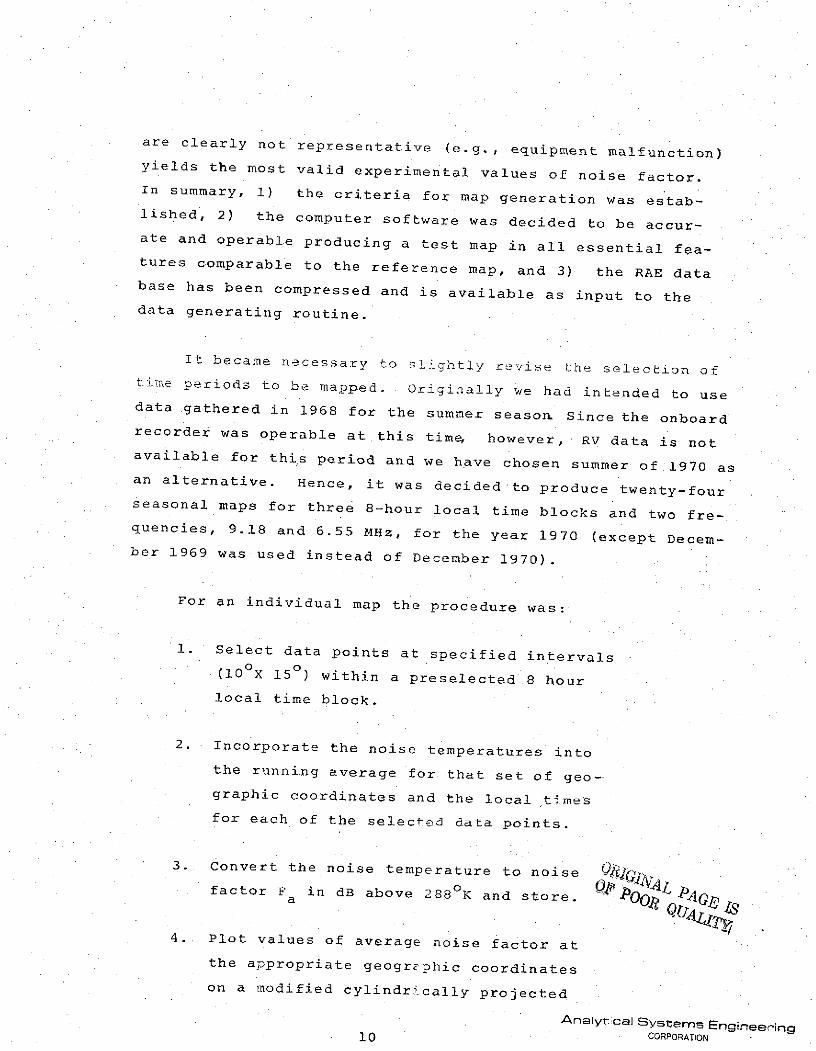
are clearly not representative (e.g., equipment malfunction)yields the most valid experimental values of noise factor.In summary, 1) the criteria for map generation was estab-lished, 2) the computer software was decided to be accur-ate and operable producing a test map in all essential fea-tures comparable to the reference map, and 3) the RAE database has been compressed and is available as input to thedata generating routine.
It became necessary to slightly revise the selection oftime periods to be mapped. Originally we had intended to usedata gathered in 1968 for the summer season Since the onboardrecorder was operable at this time, however, RV data is notavailable for this period and we have chosen summer of 1970 asan alternative. Hence, it was decided to produce twenty-fourseasonal maps for three 8-hour local time blocks and two fre-quencies, 9.18 and 6.55 MHz, for the year 1970 (except Decem-ber 1969 was used instead of December 1970).
For an individual map the procedure was:
1. Select data points at specified intervals(10 0 X 15 ) within a preselected 8 hourlocal time block.
2. Incorporate the noise temperatures intothe running average for that set of geo-graphic coordinates and the local times
for each of the selected data points.
3. Convert the noise temperature to noise s4 ~factor F in dB above 288 K and store. P00~ 4 G&
4.. Plot values of average noise factor atthe appropriate geographic coordinates
on a modified cylindrically projected.
Analyt:cal Systems Engineering10 CORPORATION
world map or other suitable projection.
5. Generate contour curves of constant noise
factor in 5dB increments.
This procedure was followed and data (i.e., actual noise
factor value) were calculated. These datawere then used as in-
put to the existing NASA contour mapping routines. Many of
the contours are not totally useful since observational pe-
riods during daylight time blocks yield scant information.
The 00-08 and 16-24 local time blocks resulted in useable con-
tours. Hence, 16 noise contour maps were obtained. The con-
tours obtained from the NASA program were not all closed due
to lack of data in certain areas. These were manually closed
and continental outlines added to the plots.
2,2 GLOBAL HF NOISE CONTOUR MAPS
Before beginning the discussion of the RAE noise level
contours and their subsequent comparison with CCIR predic-
tions, a brief description of the general features of the
CCIR noise predictions will be presented.
In general, there is pronounced noise activity over
the continental land masses where it is well known that
abundant thunderstorm activity occurs. Over the northern
and southern ocean regions, the noise levels are consis-
OP POOR QUAuLIT
11 Analytical Systems EngineeringCORPORATION
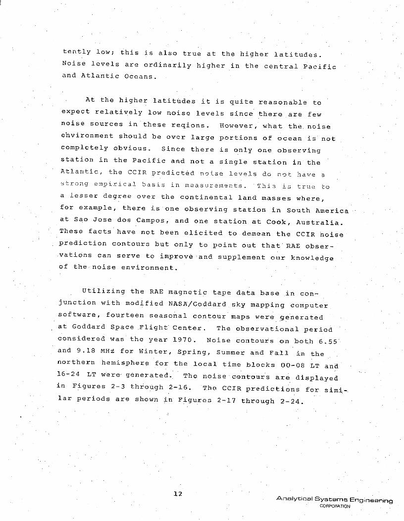
tently low; this is also true at the higher latitudes.
Noise levels are ordinarily higher in the central Pacificand Atlantic Oceans.
At the higher latitudes it is quite reasonable to
expect relatively low noise levels since there are few
noise sources in these reqions. However, what the noiseehvironment should be over large portions of ocean is notcompletely obvious. Since there is only one observing
station in the Pacific and not a single station in theAtlantic, the CCIR predicted noise levels do not have astrong empirical basis in measurements. This is true toa lesser degree over the continental land masses where,for example, there is one observing station in South Americaat Sao Jose dos Campos, and one station at Cook, Australia.These facts have not been elicited to demean the CCIR noiseprediction contours but only to point out that RAE obser-vations can serve to improve and supplement our knowledge
of the noise environment.
Utilizing the RAE magnetic tape data base in con-junction with modified NASA/Goddard sky mapping computer
software, fourteen seasonal contour maps were generated
at Goddard Space Flight Center. The observational periodconsidered was the year 1970. Noise contours on both 6.55and 9.18 MHZ for Winter, Spring, Summer and Fall in thenorthern hemisphere for the local time blocks 00-08 LT and16-24 LT were- generated. The noise contours are displayedin Figures 2-3 through 2-16. The CCIR predictions for simi-lar periods are shown in Figures 2-17 through 2-24.
12 Analytical Systems EngineeringCORPORATION
Insofar as'was possible, the contours as graphed by
the computer plotting software were not modified since it
was judged that this would insure against any preconceived
notions insinuating their way into the contours. This is
an important consideration and the results of adopting this
policy become evident when the RAE and CCIR maps are com-
pared. The CCIR contours are smooth; there are very few
anomalies; the high noise source concentrations are where
one would expect and they remain localized over the con-
tinental land masses from season to season; the contours
are always of similar shape over Northern and Southern
Ocean regions. In short, the CCIR predictions are "pre-
dictable." On the other hand, the RAE contours, while re-
flecting many of the gross characteristics exhibited in
the CCIR noise predictions, are more disjointed and dis-
play on occassion high noise levels over oceans and at the
higher latitudes. Furthermore, the contours are not as
uniform from season to season, nor are they as smooth and
"continuous" as the CCIR maps.
In some instances it was necessary to close or com-
plete contours which were unfinished by the plotting rou-
tine primarily as a result of gaps in the data. In all
cases but one it was possible to legitimately close the
contours on the basis of the trends-idicated by neigh-
boring data points supplementd by insight into thiunh--
ology of terrestrial radio noise. This was not possible
for the Spring contours for the 0-8 local time block due
to the paucity of Northern Hemisphere data.
Figures 2-5 and 2-6 depict the Spring contours for
13 Analytical Systems EngineeringCORPORATION
the local time block from 00-08 LT at the frequencies 6.55
and 9.18 MHz respectively. Considerable data is lacking
in the northern hemisphere but the contours are complete
enough to illustrate a number of interesting features.
The high noise levels over South America and portions of
Africa and Madagascar are expected, although the South
American peak level is much further south than anticipated.
The low noise levels in South Pacific and Atlantic Oceans
are also predictable using CCIR as a standard of compari-
son although the contour structure is quite different. It
is worthwhile reiterating that the impulse to modify the
contours was firmly resisted. Since there is nothing really
sacrosanct about the contouring routines and, in some cases,
there appeared to be sound reasons for rejecting the manner
in which a particular contour was drawn, this precept was,
at times, difficult to accept. However, as indicated earl-
ier, the contouring routines are consistent and objective,
and the appearance of sound reasons may simply be a guise
for preconceived notions of how the contours should appear.
A unique feature of Figure 2-6 is the high noise level
over China extending a considerable distance into the Pacific
Ocean. This structure is not predicted by CCIR and is
thought to result in large measure from HF transmitters
located on the Chinese and Russian mainland. An iono-
spheric "iris" of sufficient diameter would allow noise
from ground based transmitters to reach RAE over these re-
gions of the Pacific.
Figures 2-7 and 2-8 represent the contours for the same
season and frequencies for the time block 16-24LT. The
characteristics are quite similar to 0-8LT contours. How-
ever, there is much more Northern Hemisphere data and Figure
2-7 manifests high noise levels over much of the U.S. Note
the high noise factor off the coast of Bri:zil over the re-
Analytical System; Engineering14 CORPORATION
gion of the geomagnetic anomaly.
Figures 2-9 and 2-10 illustrate the summer contours
for the 0-8LT block at 6.55 and 9.18 MHz. Figure 2-10
is strikingly similar to the CCIR noise predictions for
the same period as witnessed by the preponderance of in-
tense noise sources over the continental landmasses and
low noise factors over ocean areas. Note the high noise
factor in the Mexico-Florida region. On the other hand,
there are significant differences, among which are high
noise levels over China, Russia, and the Northern Pacific.
Additionally, the noise power is of greater magnitude in
the Northern Central Atlantic. The high values of noise
power between 400 and 600 south latitude are possibly the
result of RF noise generated in the magnetosphere. Again,
notice the high noise factor in the neighborhood of the
South Atlantic anomaly in both figures.
The contours shown in Figures 2-11 and 2-12.for the
summer season and the 16-24 local time block exhibit fea-
tures like those of the 0-8LT time block. An important
feature depicted in Figure 2-11 is the high noise level at
70 south latitude and 3270 east longitude over the region
of the South Atlantic geomagnetic anomaly. The noise fac-
tor is some 10 dB higher at this geographic location than
in any of the surrounding regions. As is well known, in
the region of the magnetic anomaly the field strength is low, al-
lowing electrons to penetrate deeper into the atmosphere.
As an electron penetrates more deeply, the probability that
scattering may change its pitch angle is increased and,
hence, the likelihood that it may impart its energy to
other particles also is incr-eased. This type of scattering
is responsible for the continous removal of trapped elec-
trons with small pitch angles. A priori, it is not clear
whether increased absorption or enhanced noise due to RF
15 Analytical Systems EngineeringCORPORATION
emission will predominant. Figure 2-11 is another instance
of an enhancement over the anomaly at 6.55 MHz.
One further feature of Figure 2-11 should be emphasized.
Our basic concern has been directed toward a comparison of
the relative locations of high and low noise power regions
with little regard to the absolute magnitude of the noise.
In fact, if one begins to compare the magnitude of the noise
indicated on the RAE and CCIR contours, the comparison is
generally favorable. By way of illustration consider the
high noise factor over Africa at 50 north latitude and 120
east longitude. The noise factor as measured by RAE at
6.55 MHz over this region is approximately 55 dB. Over the
same geographic location, for the equivalent season and time
block, the CCIR predictions (Figure 2-22) indicate a noise
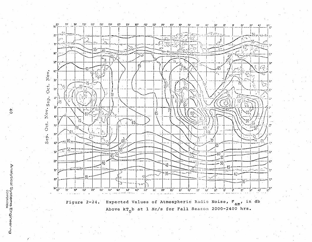
factor of approximately 90 dB at 1 MHz. Using Figure 2-25,
the noise factor at 1 MHz can be scaled to its appropriate
value at 6.55 MHz. At 1 MHz one chooses the value 90 dB to
select the correct parametric curve. Moving down the curve
to the value 6.55 MHz on the abscissa, a value of Fa equal
to approximately 56 dB is read on the ordinate. This is a
rather favorable comparison. The example also helps to make
manifest the close kinship between the RAE contours and CCIR
predictions in regions where there is agreement. Because of
the different naturesof the contours, and the invariably
consistent contrast between high noise levels over the eq-
uatorial landmasses and low noise levels over the oceans in
the case of the CCIR predictions, the similarities between
RAE and CCIR are somewhat obscured. This is somewhat.the
situation of Figure 2-11 where the high over Africa, which
is equal in magnitude to the CCIR predicted value, is less
obviously visible since the noise factors in the neighboring
ocean regions are of comparable value and the shape of the
local contours do not instinctively' cause the eye to focus
on the African high. The facts illuminated by this discourse
16 Analytical Systems EngineeringCORPORATION
can be easily duplicated in many other instances, and the
reader may reaffirm these facts with very little difficulty
by repeating this process using almost any of the RAE con-
tours over locations where there is a general correspondence
of gross characteristics for both the RAE and CCIR contours.
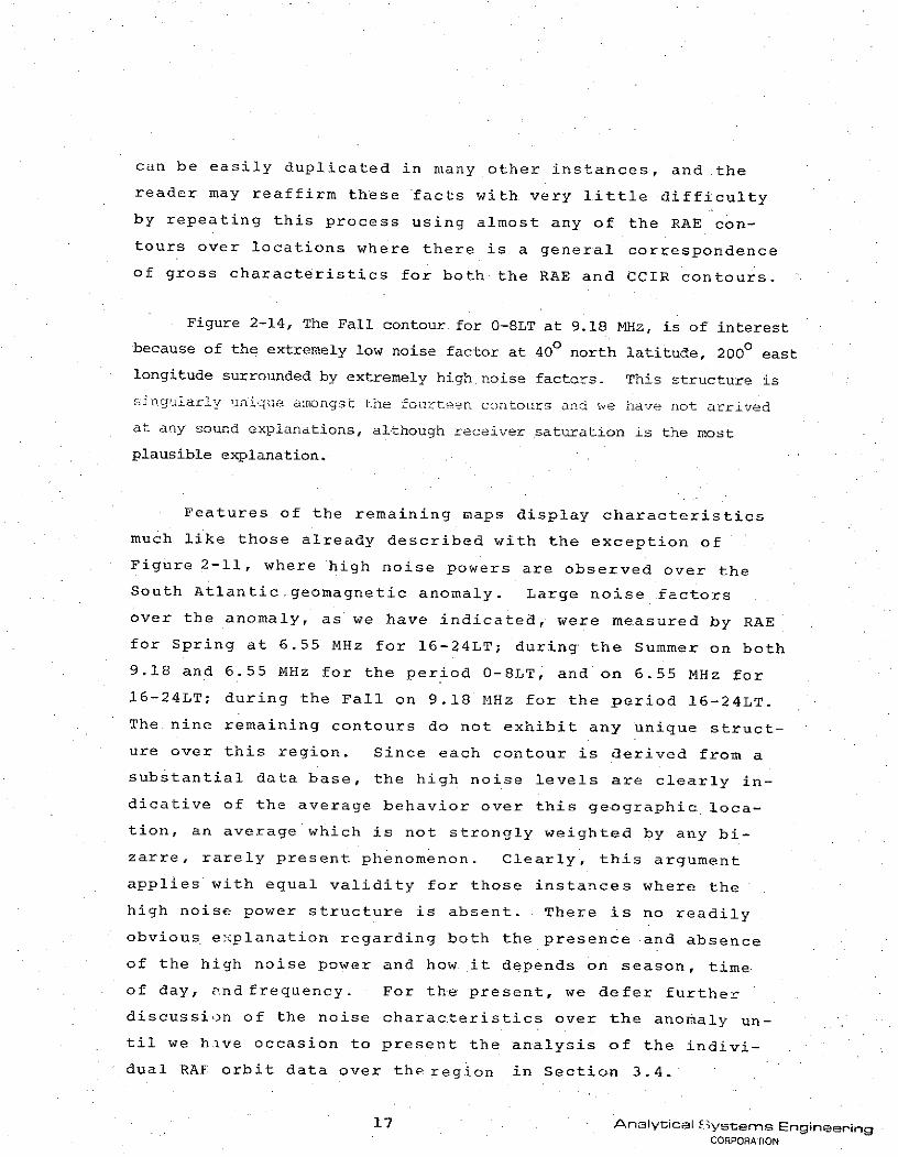
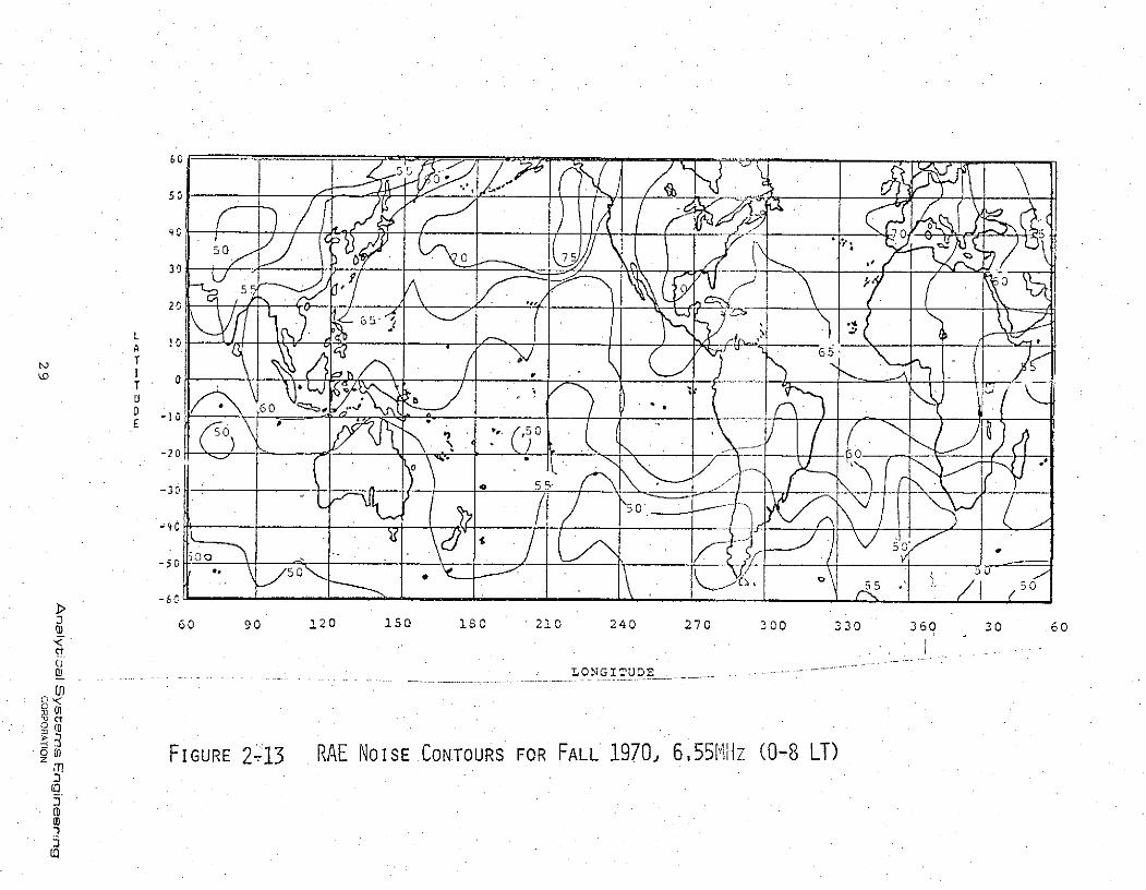
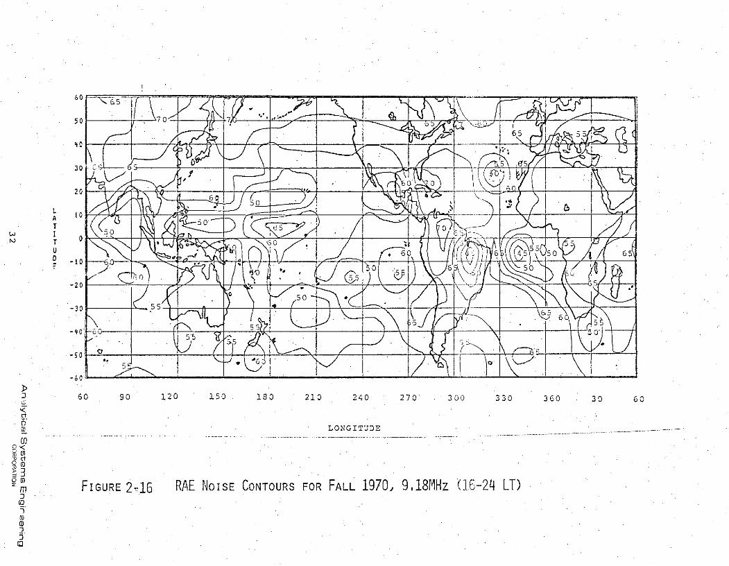
Figure 2-14, The Fall contour for 0-8LT at 9.18 MHz, is of interest
because of the extremely low.noise factor at 400 north latitude, 2000 east
longitude surrounded by extremely high noise factors. This structure is
singularly unique amongst the fourteen contours and we have not arrived
at any sound explanations, although receiver saturation is the most
plausible explanation.
Features of the remaining maps display characteristics
much like those already described with the exception of
Figure 2-11, where high noise powers are observed over the
South Atlanticgeomagnetic anomaly. Large noise factors
over the anomaly, as we have indicated, were measured by RAE
for Spring at 6.55 MHz for 16-24LT; during the Summer on both
9.18 and 6.55 MHz for the period 0-8LT, and on 6.55 MHz for
16-24LT; during the Fall on 9.18 MHz for the period 16-24LT.
The nine remaining contours do not exhibit any unique struct-
ure over this region. Since each contour is derived from a
substantial data base, the high noise levels are clearly in-
dicative of the average behavior over this geographic loca-
tion, an average which is not strongly weighted by any bi-
zarre, rarely present phenomenon. Clearly, this argument
applies with equal validity for those instances where the
high noise power structure is absent. There is no readily
obvious explanation regarding both the presence and absence
of the high noise power and how it depends on season, time
of day, and frequency. For the present, we defer further
discussion of the noise characteristics over the anomaly un-
til we hive occasion to present the analysis of the indivi-
dual RAE orbit data over the region in Section 3.4.
17 Analytical Systems EngineeringCORPORATION
The RAE noise contours, we feel, represent a valuablecontribution to our knowledge of the terrestrial noise en-vironment and we wish to re-emphasize and summarize theirsalient features. In many respects the contours comparefavorably with the CCIR predictions, exhibiting, in general,high noise factors over the continental land masses and lownoise levels over ocean regions. Where they differ, thereare reasonable explanations in most instances. For example,the high noise levels over some portions of the ocean and theEast Asian mainland are very likely accura- -representationssince they are firmly grounded in empirical data. The CCIRpredictions are based on little or no data, and thereforesuspect. The enhanced noise levels at high latitudes areattributed to magnetospheric emission processes, and there-fore are not representative of the noise power on Earth's
surface.
In those cases where no acceptable explanation of thenoise structure is forthcoming, it is not necessary thatthe RAE results be repudiated. We emphasize once again thatthe contours are based on observational data, and theoreti-
cal predictions not verified by empirical data can becomethe bane of knowledge if the theory is ultimately shown tobe inaccurate; consequently our reliance on empirical data.
The RAE HF noise contours, we contend, have expandedour knowledge of the terrestrial noise environment and arean important source of empirical observations over thoseglobal regions which heretofore have proved to be inaccessible.
The RAE contours supplement and enhance the CCIR worldwidenoise predictions and therefore will be of importance toboth the scientific researcher and the communications sys-tem designer.
18Analytical Systems Engtneering
CORPORATION
60 0 0_
50
30
50
60 90 120 50 0 210 240 270 200 330 360 30 6070
W LONGITUDE
ut
FIGURE 2-3 RAE NOISE CONTOURS FOR WINTER 1970, 6.55M-z (0-8 LI)m
(D37.
-20
-30
-40
mi IUR -
60
50
E~ -70
.F M30
20 - 5-
L _ _AT
r-7 n
T
3
C1
E
-2
03
16 56 G
ow
rr
.50
-60
<60 90 120 ~10 180 210 240 270 300 330 3§00 30 60
LONGITUDEcn ...
SFIGURE 2-4 RAE NOISE CONTOURS FOR WINTER 1970, 9,18M1H z (0-8 LT)
S... .LONGITUDE
O W
005
:3
FIGURE 2-5 RAE NOISE CONTOURS FOR SPRING 1970, 6.55MHz (0-8 LT)2
-3 J ,
IDFGR - A OSECNOR O PIG190 ,jF5 08J
No DAA
3 -0
20
60 90 120 150 180 210 240 270 300 330 3 560 60
0
-2 5 -7C,
-)
m_ FIGURE 2-6 RAE NOISE CONTOURS FOR SPRING 1970, 9,18lHz (0-8 LT)
(0
50
5
60 90 120 150 180 210 240 270 2 00 330 360 30 60
01 LONGITUDE
A 5
*m
0T
(D
-0
0
(D
2.5
50 A0
50
30
20
L
A 10
M
T 55 A-
S4-605 60
u
,
0 65
-50(
,FIGURE 2-8 RAE NOISE CONTOURS FOR SPRING 1970, 9. 18MI-1z (16-24 LT)
5550 0
30
20
150
A 10
T5
T 5 -- RM0 ________
-20
-30
c ) ------
CD~
12 5 8 1 4 7 0 3 6 0 6
60
30 .5 T
b V-O
30
20 Y : 5 J - °
Ct
1 O 020 150 iS 101
00
(50
D -60
5o
((3
.50
'C
30
u 5
M -0E
odo
0'
2O(
I 0 _ _ -7 0 5
30
t-
LONGITUDE01
SCt
43
o3 (
-0
m
-3
tfl5
50
50
~9 L -O NG ,
I ,
O
hu
:3
CD
'55
:3
60
50 _
* 60 90 120 150 180 210 240 270 302 330 360 30 60
03 LONGITUDE0
zm1SFIGURE 2-14 RAE NOISE CONTOURS FOR FALL 1970, 9,18MHz (0-8 LT)-D
o6
-:3
(0
x 5I'I / IVU
4- 3"0 inS
Z6m0 _ ~I X1 5
FIUE21 A NIECNOR ORFL 90 .1Mz('- T(Dn Il,
60
504
00 5
45
30 - 4
3020
T 0
-20too
-20
t 6 90 120 150 190 210 240 270 30 330 360* 30 60
0 (<
FIGURE 2-15 RAE NOISE CONTOURS FOR FALL 1970, 6.55 lz (16-24 LT)no
3 0 ---- -- -
60
50. -
20
-3
5-50
2 60-90010 1N0 210 2AL 290 300 330 336
z6
T0D
C5
-32
0(0
(D
T ' 3s . 2' 5 M 1,? 1 65' 0 13 ' U 23' 1 ? ( ' 05' " 'S' 7' 4P 1:V
-0 46
2 - - .r
n - ... ...
V _2V --- -- '-
It
()
Figure 2-17. Expected Values of Atmospheric Radio Noise, F in db2 I jam' "
3 Above kT b at 1 Mc/s for Winter Season, 0400-0800 hrs.
3
aC) irii ~2{ 7 h35 3 3 3' 13 3' Cs S S S 3' 2' )S 2 s ' ~ ~ 3' ~ 5' 33' 4? CS'
-JiJ -rt~
:3w
CIA S I' ' 1C' I3 7' S E' IV 1W 1 ( I Ir V 45 E? y? V t ,
I -rV15 . I i i.. ,
4 7 > _ { . ; ,- A. J2 .''2 _. ':-.-;- -:'' '-' '
- . -i C.i?-
q55.
UW 70- . I ; -
-T--- I--- - -
-i I-- !~ L I 0
I" - UUU a560I 80 C _
____ -----: ...
i4 5
o ,<l ... .. .... .. . .LuU -?: H::
-oc-t
oR Figure 2-18, Expected Values of Atmospheric Radio Noise, F.m,inb
_ 3Above kT b at 1 Mc/s for Winter Season, 2000-2400 hrs.
Figure 2-22. Expected Values of Atmospheric Radio Noise, F in dbam
a-~
M Above kT 0b at 1 Mc/s for Summer Season, 2000-2400 hrs.10
(D2(
' I 0 t ' 1 150' 0 13 5' V 5 0* 7 t 4' 3' 15' C IS' 30 ' 45 '300- - ... .. -..... .-
I ..-_I ..... i -- I :,
i _' ___
TV-t 7 C (-
..... .. B55 ~"~- I
o ....... 20
n0'0
r r)
03 I -
(0+o7
Above Tb at 1 Mc/s for Fall Seaon, 0400-0800 hrs.
(04
0 (D5Fge -3 EeeVlsftsh iRiNi ,i+
0 U) azYM Above kT b at 1 Mc/s forFall Season, 0400-0800 hrs
D 0:
(D 2
CoS' 5' "P 15' IZ03' " 5 CS' M IS' I ' O 105' 10' 70 5' c% I' Co 4' 11 q'
o'. " -I '
7 '
4 j
Sri'
lfr 1 -
i e - x t au
n' . -- - '--* - - ----- -
o 0
_. . .., _ _ . .
I~~~~~~- -i l ~ i_ -
..D
t' -- +--"--- J .
0 T-TJI--A Q - ' I - - - ,! I, i
", ",'c ,i I
I ' --I-
Epcted Value of A t pic Noise
20 i vI IIFigure 2-25. .Variation of Radio Noise with Frequency
-- I - l i d I.'il- - ------ ....
41 Analytical Systems Engineering
- E .I c'd V a 1 .a'.t.'<d .c i i -.
Sumime Sao 2 hrs.-- i ii- -l
41 Analyticel Systems EngineeringCORPORATION
3.0 SPECIFIC GEOPHYSICAL PHENOMENA
Analyses of the RAE I noise data (Herman, Caruso and
Stone, 1973) have shown the importance of the location
and strength of terrestrial noise sources upon the noise.
level in near space, Just as important has been the
ionosphere intervening between the terrestrial noise
source and the satellite receiver. This was emphasized
on data taken as the satellite approached a region of low
peak ionospheric electron density or low critical frecuency.
The terrestrial noise was seen to increase on successively
lower frequencies as received by RAE, producing the typical
"ground breakthrough" pattern.
Other ionospheric phenomena besides the sunrise/sunset
terminator, were chosen to consider their effects on
terrestrial noise as seen by RAE. The ionospheric features
analyzed were chosen because their spatial location is well
established. These phenomena are: the midlatitude trough
(Muldrew, 1965); Polar Cap Absorption (PCA) events (Bailey, 1964),and the South Atlantic Magnetic Anomaly (Dessler, 1959).
Each of these is a well defined area where there is an
obvious variation in either the F-region or D-region electron.
density compared to the surrounding area. Decreased F-region
densities, as in the trough, or increased densities of the.
magnetic anomaly will be detected through the spatial
variation of the ground breakthrough. D-region enhancements
caused by a PCA event or perhaps originating in the magnetic
anomaly will produce a decrease in signal strength due to
the resultant non-deviative absorption in the enhanced
D-region. The F-region and D-region effects can result in
similar effects upon the RAE data. Thus, it will be the
spatial variation of the data that will reveal the location
of the geophysical phenomena. However, determining whether
42Analytical Systems Engineering
CORPORATION
one is seeing an F-region or D-region effect will be difficult
if not impossible.
The effects described are tied closely to the Earth's
magnetic field and energetic particles, electrons and
protons that are guided to ionospheric heights from space
by the field. These particles can be emanating sufficient
RF energy in the frequency range of the RAE data to be
detected. The most obvious location of such an effect will
be the auroral oval. Data taken on trajectories through the
oval will be examined-. Use of both upper and lower Vee
antennas will help establish whether any noise detected is
coming from the Earth's surface or ionospheric heights or
greater. Since the enhancements in the South Atlantic
Anomaly are thought to be due to particle precipitation, this
will be examined also.
It is convenient to separate the analysis into two
parts.. The first concerns high latitude effects (the PCA,
auroral oval and the mid-latitude trough). These three
compose adjacent regions that extend from the pole to the
magnetic L shell of L = 3.5. We will examine the RAE
data for ionospheric effects and magnetospheric noise
sources. The South Atlantic Anomaly will then be examined
both for ionospheric enhancement and noise sources. An
experiment was also performed to generate an artificial
aurora during a time when RAE data was available (Hess, et al.
1971). This will be examined for increased RF emissions
due to the artificial aurora that might be detected by RAE.
3,1 HIGH LATITUDE PHENOMENOLOGY
The polar cap, auroral oval and finally the mid-latitude
trough make up an integral ionospheric-magnetosph ric region.
Analytical Systems Engineeri igCORPORATION
These three effects appear to be related r or have a common
cause, through the Earth's magnetic field. Whereas their
locations above the Earth's surface are related, their time of
occurrence is somewhat separated, The PCA occurs often
during magnetically calm periods when there is little
significant auroral activity in the auroral zone. The mid-
latitude trough is consistently present. Each of these will
be discussed briefly in the following paragraphs as individual entities.
One should remember their spatial relation to each other and
their relation through precipitating particles. These
effects will first be examined as an ionization anomaly
with emphasis on the PCA and trough. Then the aurora will
be examined as a source of RF emissions,
3.1.1 THE POLAR CAP ABSORPTION EVENT
While there are many ionization sources affecting the
polar cap, that which is to be examined here is the
enhanced ionization, particularly in the D-region, which is
produced by the invasion of solar cosmic rays a few hours
after a solar flare.
Occasionally a solar flare will give rise to intense
fluxes of energetic protons that precipitate into the
upper atmosphere over the polar caps and auroral oval. The
protons will also be accompanied by some electrons and
heavier nuclei such as a-particles. The geomagnetic field
determines the minimum energy that a given species must
possess in order to reach the Earth at a particular point.
This filtering effect results in the lowest-energy particles
having access only to the polar caps.
The actual process of ejection of solar cosmic rays is
not well understood. Those producin a PCA are ejected
44 Analytical Systems EngineeringCORPORATION
during or shortly after a type IV radio noise burst and
associated optical flares. Flares associated with high
energy events tend to lie to the west of the central
meridian of the sun. Flare locations near the west limb or
even beyond appear most favorable.
The ejected particles appear to travel to the Earth
by paths which are usually several times larger than the
Earth-sun distance. These two facts conform to the Archimedian
spiral structure of the interplanetary magnetic field, which
magnetically guides the solar particles from the source to
the Earth. This field also appears to store the particles.
The ejection process is thought to be short but the PCA
duration may be measured in days. The Earth's magnetic field
is greatly distorted by the solar wind. As a result the modes
of particle entry into the polar cap should be different from
those anticipated from the Stormer theory for the dipole geo-
magnetic field.
The development of the PCA is a three-step pattern. The
first stage is a slight increase of absorption near the geo-
magnetic pole. Next, it develops within the latitude of 650.
Finally it extends down to about 600. The fully developed
PCA has circular symmetry in corrected geomagnetic coordinates,
giving a definite cut-off latitude. This has been explained
by the existence of a ring current whose magnetic moment must
be .4 that of the Earth. It also appears that the solar protons
have immediate access to the polar caps because the polar cap
field lines merge with the interplanetary field. It would be
natural to expect the shape of the PCA area to be oval, reflect-
ing the day-night asymmetry of the auroral oval. Synoptic analysis
of PCA has shown a symmetric pattern of particle precipitation.
There is, of course, a diurnal variation of a PCA due to sun-
light which is reflected in some records, such as riometer
absorption.
45 Aralytical Systems EngineeringCORPORATION
There are anamalous F-region electron densities in the
polar cap, specifically troughs and peaks. The troughs ex-
ist mainly on the night side and lie along magnetic isolines.
A peak of electron density is observed around geomagnetic
noon at 780 invariant latitude. The ionospheric effect of
interest here however is the increased D-region electron den-
sity that results from the impinging solar protons. The re-
sulting polar-cap absorption, caused by the increased non-
deviative absorption in the D-region, can possibly reduce
the noise intensity from terrestrial sources when the RAE is
over the polar cap.
The methods of calculating the electron density follow
the physical process closely and reveal the process of con-
verting high energy protons to an increased electron density.
The first step in the process is to determine the energy loss
of the protons at each height within the ionosphere and ex--
press this as the volume electron-ion pair production rate as
a function of height. Early attempts at this required that
the energy spectrum of the particle flux be assumed. Normally
exponential or power-law spectra were assumed as was the cut-
off energy. It was demonstrated that the exponent was re-
latively unimportant. Most electron production depends upon
the protons just above cutoff.
Once the production rate profile is determined, the el-
ectron density profile can in most PCA cases be calculated
assuming no other source of ionization. The contribution of
that part of the profile above 85 km to the absorption is in-
sicnificant. It is recognized that the enormous difference
in absorption between day and night during the PCA can be
exolained if negative ions are found by electron attachment
at: night and photodetachment of electrons by day. Typical.
n-,ght and day profiles during a PCA are shown in Figure 3-1.
46 .Analytical Systems EngineeringCORPORATION
110
90 -
(a) o /-o
0 10 0 l0
ELECTRON DENSITY (c r-)
110ELETRN ENSIY (cm-)90-Figure 3-1 Height profiles of electron density
20 MEV and 40 MEV. (Reid, 1961)
47 Analytic.I Systems EngineeringCORPORATION
The ability to measure the radiowave absorption that
results from the electron density using riometers, and the
ability to measure the proton spectra above the ionosphere
has led to much work in evaluation of the energy deposition
and the various rate coefficients believed to be involved.
The riometer, which measures the absorption of galactic noise.
as seen from the Earth, reveals the effect one expects to see
of the absorption of terrestrial noise as viewed from space..
Most riometers are operated at the same frequency, 30 MHz,
to allow comparison between observations. Data taken at Thule,
Greenland for two PCAs is shown in Figure 3-2. In the first
illustration a diurnal variation can be seen, of up to an or-
der of magnitude variation of the dB absorption from day to
night.
RAE DETECTION OF PCAs
The absorption as a function of frequency has been found
to vary as
nA(dB)=C(f-f L) (3-1)
L
where f is the receiving frequency, fL is the longitudinal
component of the electron gyrofrequency. The constant, C,
varies with the intensity of the event and the exponent n
varies from 1.1 to 1.9 depending upon the proton spectra.
Using this relation we can convert the reported riometer ab-
sorption at 30 MHz to the RAE frequencies. This will indicate
the amount of absorption to be expected when the satellite
passes above the polar cap. At the highest frequency, 9.18 MHz,
the absorptior in dB will be from 3. to 10 times that at 30 MHz.
At 2.2 MHz it would increase to at least 14 to 43 times that
at 30 MHz. This increase in absorption at low frequencies
combined with measured 30MHz absorption of 10 to 16 dB during
some events makes one optimistic that seeing the effects of a
48 Analytical Systems EngineeringCORPO "ATON
10
I-
Univ. time
; 12 24 i2 2'4 .2 2 -
Sept. 2,!966
Figure 3-2(a) Plot of dB absorption vs. time for the PCAevent of 2 September, 1966, as observed at Thule Greenland,on the 30MHz riometer. The nighttime recovery in absorptionis immediately noticeable (from R. Cormier, private communi-cation).
Figure 3-2(b) Plct of dB absorption vs. time for the PCA eventsof 24 May and 2S May 1967 as observed at Thule, Greenland, onthe 30MHz riometer. There is no nighttime recovery since atthis season the sun does not set in this region (from R. Cormier,private communication). (Silverman, 1970)
49 Analytical Systems En ineeringCORPORATION
PCA on the RAE data is a sure thing. Such is not the case and
analysis of the data will have problems. First, since the or-
bital inclination is 1210 the satellite only reaches geographic
latitudes of 590. Therefore interception of the polar cap will
be most likely on those orbits over the eastern United States
and Canada, in particular when the orbital plane is such that
the northern most point of the trajectory crosses the longitude
of the Earth's corrected geomagnetic pole at about 81°W geo-
graphic. On this optimum trajectory through the. polar cap the
northern :most geomagnetic latitude wi l be 730, well within the
PCA lower latitude limit of 60. On the oooosite side the satel-
lite. would only reach 450 geomagnetic latitude and be outside
even the auroral zone.
It has already been noted with respect to the maps of
terrestrial radio noise created from the RAE data that noise
sources are not expected at high latitude. In the winter, few,
if any, thunderstorms are expected to occur at latitudes (geo-
graphic) higher than 300. Further, the large maximum over the
whole of Europe and Asia are far removed from the Polar Cap
due to the eccentricity of the magnetic dipole. Thus it seems
that any noise leaving the Earth at polar cap latitudes will
have first propagated from other sources before escaping, per-
haps through one of the polar troughs. These sources could
havebeen many thousands of kilometers from the satellite
nadir and any D-region penetration occurred far removed from
the PCA effected D-region. We must guard our optimism before
searching for PCA effects on the RAE noise data.
50Analytical Systems Engineering
rr r -,
3.1,2 MIDLATITUDE TROUGH
The introduction of ion trap experiments aboard Sputnik 3
allowed the direct measurement of electron density at iono-
spheric heights rather than indirect measurement by ground
based radio techniques. A variety of experiments since have
shown the ionosphere not to be describable by sweeping gene-
ralities. It is not a smoothly varying medium. Most of the
irregularities however have been shown to be aligned with
the geomagnetic field. One of these irregularities has be-
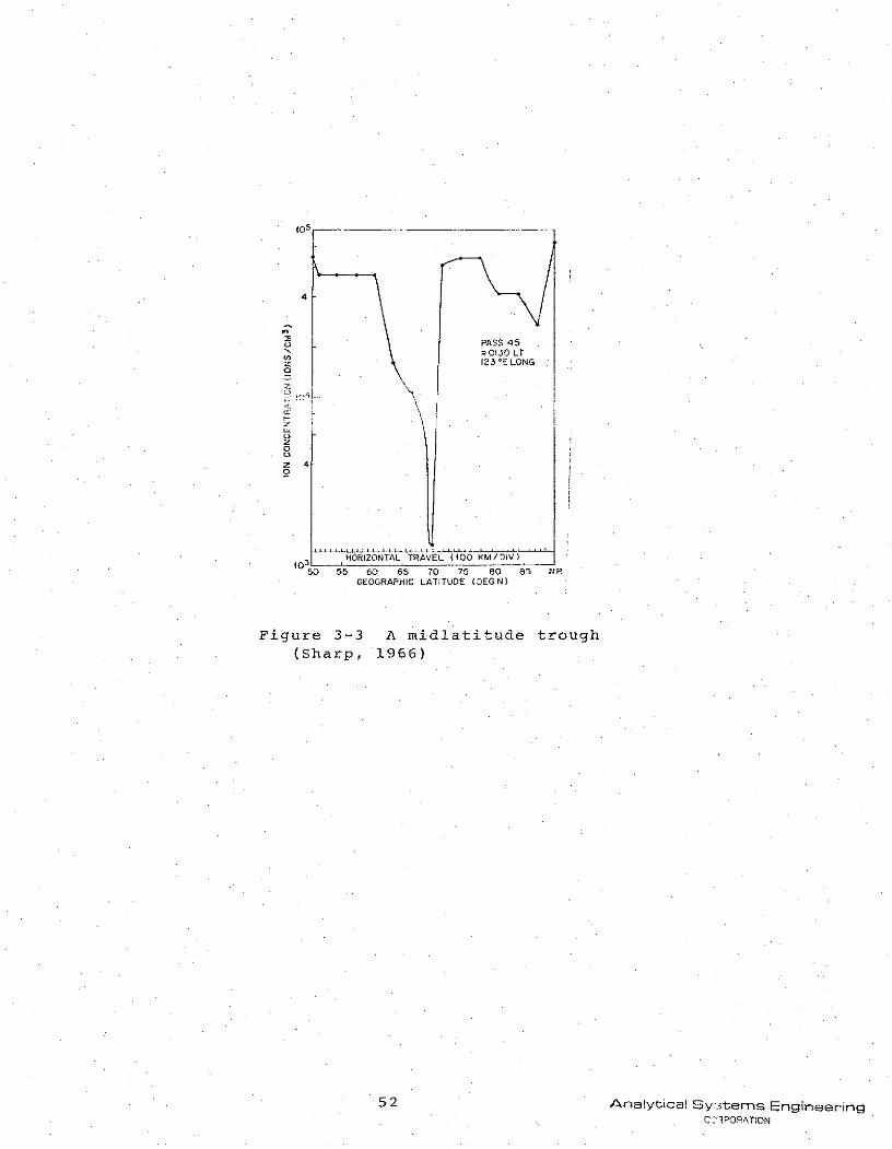
come known as the Midlatitude Trough (Muldrew, 1965; Sharp, 1966).
The midlatitude trough as shown in Figure 3-3 reveals
itself on satellite measurements of ion concentration as
sharp decreases in ion density of an order of magnitude.
This decrease occurs both above and below the F-region peak
(Figure 3-4) and can be assumed as a reduction in the electron
density of the whole F-region as well as a reduction of the
critical frequency. The trough is found surrounding.both
the north and south magnetic poles. It is most. evident at
night since solar radiation can tend to "fill" the trough.
The poleward side of the trough normally has a much greater
gradient, often being an abrupt step-like increase in elec-
tron density as in Figure 3-3. The trough is not located in
the auroral zone but borders the equatorial.side of the
auroral zone and will be affected by auroral activity. The
trough becomes very narrow during periods of high magnetic
index and auroral zone particle flux increases. This is
mostly due to the poleward wall. which is the auroral zone,
moving equatorward. The equatoral wall of the trough re-
mains in a somewhat stationary location as seen in Figure 3-5.
The cause of this trough is not clear. One theory is
that the trour:h is the ionosphere that would exist if solar
MID LATITUDE TROUGH HALF WIDTH POSITION. MID LATITUDE TROUGH. HALF WIDTH POSITION,NIGHT 16 31. LOW PRECIPITATED FLUX. NIGHT 58 73. HIGH PRECIPITATED FLUX.AVERAGE ,(>8O eV) 085 ERGS/CM
2 /STER AVRG >0V 3 RSC2 /STER
Figure 3 5 Polar plot comparison of trough half width
and flux precipitated in the auroral zone. (Sharp,966)
54 Analytical Systems Engineering
COrHPoATION
radiation were the only energy source. The increased den-
sity on either side of the trough then would be caused by
corpuscular radiation. Since the location of the trough at
L=3.5 is the same as Carpenter's "Whistler Knee", it has been
suggested that the knee mechanism is responsible for the equa-
torial side of the trough and the particle precipitation
in the polar auroral zone for the poleward side.
It has also been suggested that the trough is due to an
ionization sink at the magnetic latitude of the trough.
Elec ric fields in the auroral and airglow phenomena would
cause heating of the ionosphere. Therefore an expansion and
a reduction of electron concentration would take place. Much
work is yet to be done to substantiate either of these ex-
planations or others.
TROUGH DETECTION WITH RAE
The trough is seen to vary from 100 to 200 in width,
described as the difference in latitude between the half-
depth points. This is approximately the maximum resolution
possible with the RAE antennas as depicted in Figure 3-6.
At the highest frequency, 9.18 MHz, the travelingwave an-
tenna has a beamwidth of 13 0 x27 0 . Thus, if the satellite
trajectory crosses normal to the trough and the sharpest
antenna pattern is aligned with the trough it may be possi-
ble to see an increase in noise, reflecting the decreased
electron density. In other words, one might expect a sharp
increase in ground breakthrough as the satellite crosses
the trough.
Howeve :, bear in mind that the one explanation of the
trough involved particle precipitation on either side of the
trough. This could cause increased noise due to synchrotron
radiation ,rior to and after the trough, masking its presence.
55 Analytical Sys ;ems EngineeringCO0 7ORATION
RAE
D. W. > 30
Re8 B. W.
Figure 3-6. RAE Spatial Resolution
5 6 Analyt;ca! Systems EngineeringCOPPORATION
3.2 RAE 1 NOISE MEASUREMENTS
It has become apparent in recent years that several ionos-pheric phenomena affecting HF radiowave propagation are in-timately related to energetic charged particle precipitationfrom the magnetosphere as discussed in Section 3.1. In additionto producing ionospheric absorption which can affect radionoise Propagating from the ground to RAE altitudes, these particlesmay produce RF emissions in the RAE band of freuen 0 ies as dis-cussed in Section 3 .3
Energetic particle precipitation takes place principallyat geomagnetic latitudes greater than about ± 600 althoughintense events associated with and following solar eruptions
may spread equatorward as low as 500 geomagnetic latitude.Phenomenological patterns of particle precipitation exhibitdiurnal and geographical variations which are similar to thoseof auroral ionospheric phenomena. Hence, we would expect theregion affecting transionospheric propagation of terrestrialnoise to RAE altitudes to be in approximately the same locationas the region of auroral RF emissions.
In the north-west quadrant of the globe centered at about81 0 w longitude, a given geomagnetic latitude is up to 110 higherthan the corresponding geographic latitude. This means thatover the U.S. and Canada auroral events can extend as low as39 N geographic latitude. On the opposite side of the world
(south-east quandrant) over Australia the same situation pre-vails, i.e., -50 geomagnetic latitude corresponds to -geographic latitude.
Considering the orbital characteristics.of RAE 1, it isevident that the satellite spends about 100 minutes of eachorbital period, or 45% of its time, over geographic latitudes
57 '-nalytical SVst=m, r-
between 40 and 600 in the northern and southern hemisphere.
Due to the displacement between geomagnetic and geographic
coordinates, RAE spends nearly 25% of its time over auroral
latitudes; so a significant portion of the RAE data can be
utilized to investigate the effects of polar cap absorption
(PCA) events, auroral substorms and the main ionospheric
trough on the RF environment at satellite heights.
On the one hand we can expect that ionospheric absorption
associated with PCA events and auroral substorms will depress
the noise contribution to RAE from sources below the ionos-
phere, while the low critical frequency found in the main trough
would allow noise on lower frequencies than usual to penetrate
through the ionospheric shield and reach RAE. On the other hand,
we can expect that noise emissions generated by the precipi-
tating particles associated with auroral substorms might enhance
the noise level at RAE heights. The relative importance of
these several competing factors has been examined.
Before presenting the analysis of noise measurement data
taken by RAE i1, we will give a brief description of the charac-
teristics of the satellite,-the Vee antennas and the Ryle-Vonberg
receivers. A more detailed discussion is given by Weber, Alexander
and Stone (1971) and Novaco (1973).
58 Analytical Systems EngineeringCORPORATION
3.2.1 SYSTEM CHARACTERISTICS
THE RAE 1 SATELLITE
The system configuration, shown in Figure 3-7, consists
of two 229 meter travelling wave Vee antennas (one directed
towards the earth, the other towards the local zenith), a 37
meter dipole bisecting the axis of the Vee antennas, and a
192 meter libration damper. The latter was installed to damp
out oscillations about the satellite's axes. The Vee antennas
operate at 9 frequencies (0.45, 0.70, 0.90, 1.31, 2.20, 3.93,
4.70, 6.55, and 9.18 MHz). Each frequency is sampled every 72
seconds, The orbit, inclination and precession rate of the
satellite were chosen to provide the largest amount of sky
coverage in the shortest amount of time. The satellite was
placed in a retrograde circular orbit at an altitude of 6,000
km with an inclination of 590 . The precession rate for this
orbit is 0.52 degrees per day. It took nearly two years to
completely map the sky between the declination limits of -60 ° .
THE VEE AND DIPOLE ANTENNAS
A travelling wave antenna was made by inserting a 600-
ohm resistor and odd fraction of a wavelength from the tips of
each of the legs of the Vee antennas. This allowed most of
the energy to be placed in the front lobes since a travelling
wave antenna suppresses the back lobes.
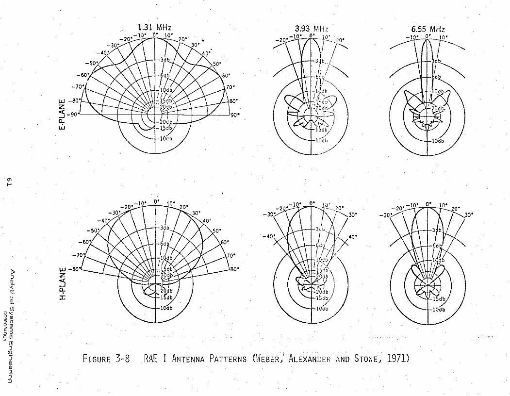
The beam patterns for a travelling wave Vee antenna are
shown in Figure 3-8 for 1.31, 3.93 and 6.55 MHz. At 3.93 MHz
the beam pattern is an ellipse 230 X 520; at 6.55 MHz, the
ellipse has narrowed to 140 X 340
Because the electrical characteristics of a simple dipole
are understood much better than the travelling wave Vee antenna,
dati from the RAE dipole have provided the basis for absolute
59 Arialytical Systems EngineeringCORPORATION
UPPER V
60"
37m DIPOLE
LOWER V
TO EARTH
FIG' RE 3-7 RAE I CONFI--URATION (dEBER, ALEXANDER 8 STONE, 1971)
60 Anliytical Systems EngineeringCORPORATION
1.31 MHz 3.93 MHz 6.55 MHz
-40 0'
-50 -3d 50 3 b
• b 60* -od
-70* 1 70- 10
-2 -80 0' " b 8at0- Odb I/ b
_,o0 , d
-1db 10b 10db
-10* 10, -10* o. -10, 10-20* 20* -2 -20A'- D D 0-30- 30* 40. -30' 30* -30* 30*
-40 404
-60* d 60* d d
-70 -1 b 70'
- db 80'
d db0) -15db -1:db 1 db
-d10.b 10b 10db
z
FIGURE .-8 RAE I ANTENNA PATTERNS (WEBER' ALEXANDER AND STONE, 1971)
sky brightness measurements of other investigations.
*Both the dipole and lower Vee are coupled to a burst
receiver which steps continuously through its frequency range.
The sweeping burst radimeter on the dipole is stepped rapidly
through six discrete frequencies from .540 to 2.8 MHz to gen-
erate a dynamic spectra. The burst receiver connected to the
lower Vee steps through eight frequencies between .245 and
3.93 MHz.
THE RYLE-VONBERG RECEIVERS
The Ryle-Vonberg receiver was chosen for RAE 1 because
it provides the required stability to make precise measurements,
over many months of unattended operation. This system
measures by a null technique and is therefore insensitive.
to internal changes in system gain or bandwidth. The re-
ceiver measures the antenna signal strength by a continuous
comparison with an internal voltage-controlled noise source
which is adjusted by a servo loop to equal the antenna signal.
This system provides a "coarse" measurement by measuring
the voltage controlling the noise source. To provide a "fine"
measurement (and also redundancy and calibration check) a
stable thermistor-bridge power meter was added to the system
which measures the output power directly from the noise source.
However, the relays. in the bridges failed after nine months.
The receiver is sampled at a slow rate, once a second
for the "coarse" measurement. Therefore, this receiver's
sensitivity is better measured by the peak of the statistical
noise instead of the rms statistical noise. This peak noise
sensitivity is =4%.
6 : AnalyticaJ Systems EngineeringCORPORATION
3,2,2 ANALYSIS OF OBSERVATIONS
To facilitate the investigation of radio noise observa-
tions in conjunction with high latitude geophysical processes,
a means was needed to plot RAE 1 satellite passes in the same
coordinate system as the auroral phenomena. This was most con-
veniently done by use of a nomographic computer which graphi-
cally converts geographical coordinates and universal time
into corrected geomagnetic coordinates and geomagnetic local
time. This nomographic computer was developed by Whalen (1970)
using the corrected geomagnetic coordinate system of Hultqvist.
The computer consists of a series of high latitude maps upon
which the mean position, size and shape of the auroral oval
can be projected for any time of day and magnetic activity..
Using the same technique, a high latitude map upon which
the mean position of the main ionospheric trough (after Herman,
1972) can be projected for any time of day and magnetic acti-
vity was also developed. The correct auroral oval map and/or
main ionospheric trough position to be used is then determined
by the magnetic activity.
The projected geographic coordinates as a function of
universal time of the position of RAE i for the various cases
examined were extracted from the ephemeral printouts described
in Section 2.1. Magnetic indices for the periods of interest
were provided by E.J. Chernosky (Private Communication) of AFCRL.
Two specific examples were chosen for discussion. The
.first is data from the PCA event which began on 2 November, 1969
at 1200 UT and ended three days later. This event resulted in
nearly the highest maximum absorption (11.7 dB on the 30 MHz
riometer as meEsured at Thule) of all the PCA events in 1968
through 1971. The data shown is representative of the winter
nighttime data that were examined and unfortunately is not
Analytical Systems EngineeringCORPC RATION
unique to PCA conditions. The second example, summer nighttime,
is from the- 1 May,.1969 PCA event (start and end times are un-
known). This was a weak event with a maximum absorption of
only .5 dB on 30 MHz at Thule.
WINTER DATA
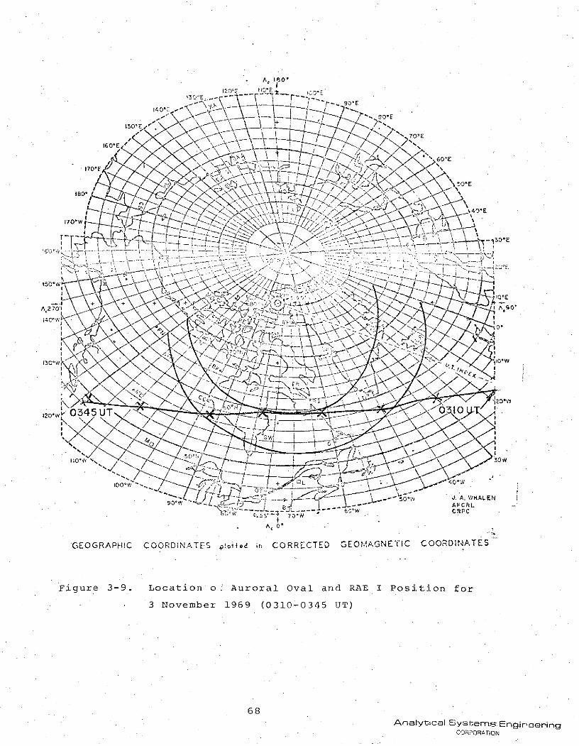
The data chosen for winter nighttime is from 3.November,
0310-0345 UT. The magnetic index for.that particular period
is given by Q=3. Knowing this and the time, defines the posi-
tion of the auroral oval. The position of RAE I is superim-
posed on the same map as shown in Figure 3-9. Plots of the
noise intensity as observed by the burst receiver are shown
in Figure 3-10. Noise intensities observed at several fre-
quencies by the Ryle-Vonberg receivers are shown in Figures
3-11 through 3-26.
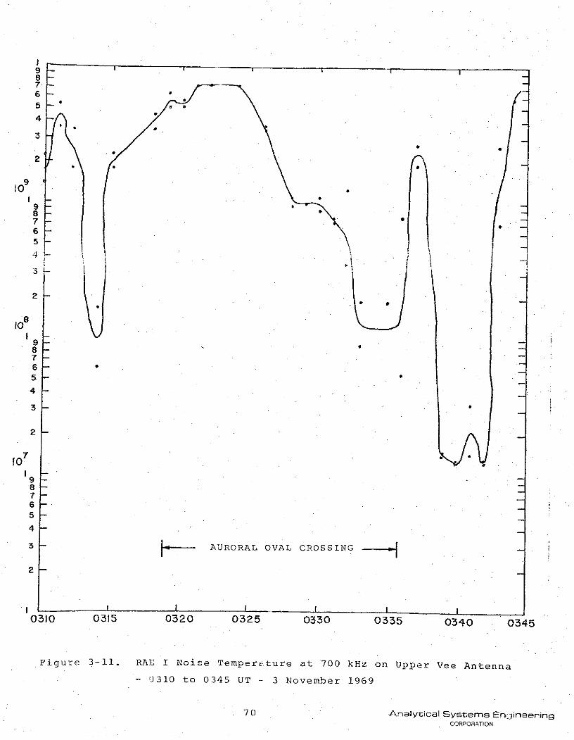
Examination of the burst receiver data shows an increase
in noise level on all frequencies at approximately the time
RAE 1 approaches the auroral oval (0315 UT). As RAE 1 passes
over the oval, the burst receiver noise levels exceed 1010
degrees Kelvin. This increase in noise intensity corresponding
to passage over the oval is often observed on other data, th6ujh
not always as clearly as in this example. Further examination
of the burst receiver data reveals that the lower frequencies
exhibit a more intense response to passage over the oval than
the higher frequencies displaying greater enhancements for a
longer time.
The noise levels a, the higher frequencies drop off sooner than
at the lower frequencies. This is the opposite of the ground
break through phenomenon observed and reported on by Herman et
al (1973).. Therefore, it would seem that this noise has its
origin above the peak of the F-layer and is not a result of the
64 Analytic;al Systems EngineeringCORPORATION
mid-latitude trough but of particle precipitation. There
certainly is not an obvious reduction in noise level due to
polar cap absorption or auroral absorption of terrestrial noise
sources within the oval.
All frequencies exhibit enhanced noise levels at least
until 0350 UT, at which time the higher frequencies returned
to their normal noise level. The lower frequencies maintained
noise levels near 1010 degrees Kelvin until nearly 0400 UT.
However, a sharp short-lived decrease in noise level is seen
on all frequencies at 0340 UT, the time the satellite leaves
the auroral region. It is possible this decrease is due to
the satellite's passing over the mid-latitude trough (which,
as stated in Section 3.1.2, borders the auroral zone on the
equatorial side) and reflects the dirth of particles in the
trough region.
A similar frequency response is observed on the R-V receiver
data. Generally speaking, the noise intensities are greater
at the lower frequencies. In this particular example, the
noise level was greatest at .7 MHz.
The R-V receiver which is connected to the upper and lower
Vee antennas could shed some light on the spatial distribution
of this noise. Examination of R-V receiver data reveals an
enhanced noise level which peaks between 0320 UT and 0325 UT.
It is stronger on the lower Vee at 700 kHz. At 900 kHz two
peaks can be seen, one about 0320 UT and a second at about
0335 UT. Again, the lower Vee noise level is slightly greater
at 0320 UT indicating t1iat the source is below the satellite.
At 1.31 MHz, the same two enhancements are observed only this
time the second peak at 0335 UT is clearly greater on the upper
65 Analytical Systens EngineeringCOPPORATION
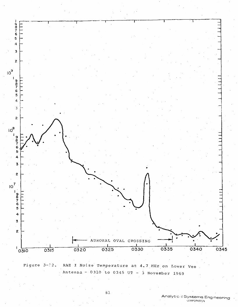
Vee antenna. At 2.20 MHz the noise intensities are greatly
reduced and at 3.93 LHz the noise peaks are no longer visible.
However, both peaks are visible at 4.7 MHz with the lower Vee
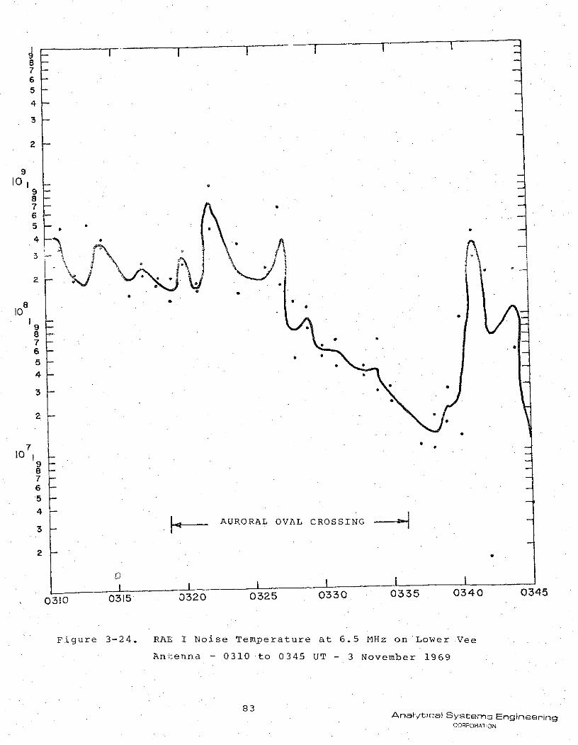
noise intensity being greater in both cases. At 6.5 MHz the
structure has again changed until at 9.18 MHz a single peak
in intensity is visible with the lower Vee noise still being
greater at about 0328UT.
SUMMER DATA
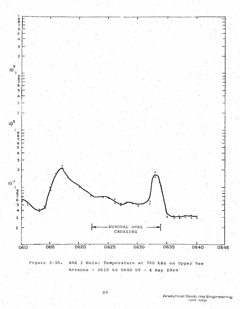
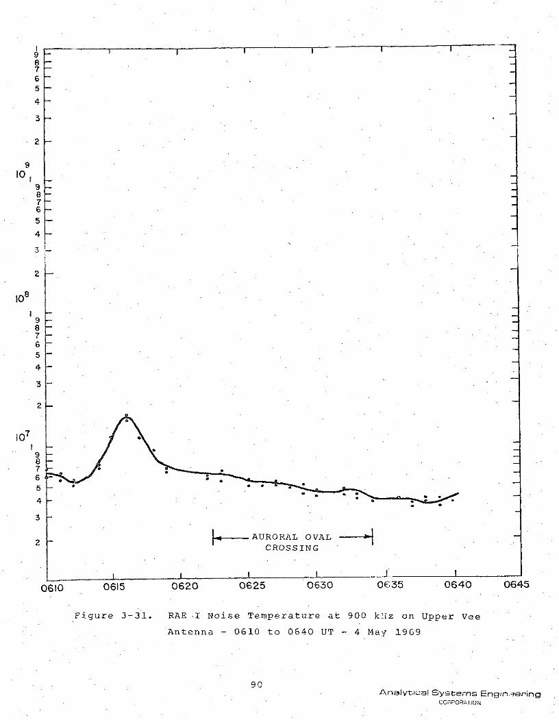
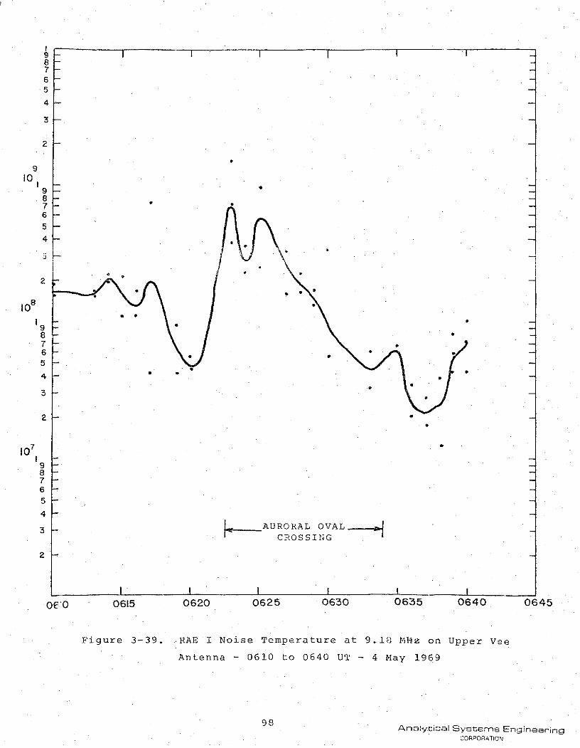
The second example is data taken on 4 May frotm 0610-
0640UT. The magnetic index is given by Q=3. The RAE 1
track superimposed on the map with the auroral oval for this
time is shown in Figure 3-27. Noise levels recorded by the
burst receiver are shown in Figure 3-28. The Ryle-Vonberg
receiver data are shown in Figures 3-29-through 3-39.
Examination of the burst receiver data between 0620-
0635UT (time RAE 1 passes over the auroral oval) shows the
greatest response occurs at .245 MHz. Noise level peaks in10
excess of 10 degrees Kelvin can be seen. Enhancements in
noise level are also seen at .328 MHz but to a lesser degree.
At .490 MHz only two spikes occur at the times RAE 1 approaches
and leaves the oval. Two spikes are seen.at 0630UT on .540
and .7 MHz. None of the other frequencies respond to passage
over the oval until we get to the highest frequency, 3.9 MHz.
While the enhanced noise level at 3.9 MHz starts to drop off
approximately 10 minutes earlier than at .245 MHz, both fre-
quencies show recovery by 0650 UT. These data are markedly
different from the burst receiver data for the winter night-
time example. The enhanced noise levels are greater in the
winter case and last for a longer time, particularly on the
lower frequencies. In the .;ummer example the enhancements
appeared only on frequencies lower than the winter low fre-
quencies, with no other response to passage over the oval
until 3.9 MHz.
66 Analytical Systems EngineeringCORPORATION
The R-V receiver data for this example is consistent
with the burst receiver data and in contrast to the data
shown in the first example. At .45 MHz, noise intensity in-
creases during the period of time the satellite passes over
the oval, with a sharp increase at 0634UT. At .7MHz (the
frequency which recorded the greatest enhancement in the
previous example), only two peaks remain at 0612 and 0633UT.
At .9 MHz only the first peak is seen. From 1.3 to 3.9 MHz,
there is no response. However, the lower Vee antenna does
show enhancements at 3.9 MHz. At 4.7 MHz, the upper Vee
measurements show some fluctuations while the lower Vee an-
tenna shows enhancements at 0635 and 0637UT. At 6.5 MHz,
many fluctuations are seen during the time the satellite
passes over the oval. Although the amount of the enhancements
differ, the general structure of the noise level at 6.5 MHz
is not unlike that seen at .45 MHz. At 9.18 MHz, the highest
frequency, the entire noise level curve is shifted upwards
and exhibits a structure entirely different from that seen
on other frequencies.
Looking at the data from either example, we have seen
fairly complicated responses over a range of frequencies.
Looking at both examples together, the data becomes even more
complex. No obvious patterns are evident except.that there
are a lot of inconsistencies. There appears to be a frequency
dependence trying to emerge that is more evident in the se-
cond example. An in-depth statistical analysis on the wealth
of data collected by RAE 1 would most certainly aid analysts
in gaining insight into what we are seeing in the data and
thus aid scientists in explaining why. Unfortunately that
level of effort was beyond the scope of this study.
67 Anal, tical Systems Engin3e ngCORPORATION
A6 100
o 2 901E
.AFCRL
3 November 1969 (0310-0345 UT)
Analytical Syste Engineering
10w 44. / i2 i 7
A--A
15 D'68
GEORAHI CORDNAESptoie i; CRRCTD EOMGNTI CORDNITE
Figre -9.Loctio o uroalOva an RA I osiionfo
3 oeme 16 (30-35 T
133"w ~T68Anaytial semsEngneeinCOPOAIO
FREn. FREQ.
S.E08 -
. '08 - - -I -
I 2EI 6.
~60
I 9 I ± "
I.E -07 . 0I.E --o- ,- L :
S1.0
I.E08 3
0 -t1.E09 -- --- --- -
I.1: I I ' II . E+ 10
.9.0
S1.E06
.E*05
1E+05
3 .
Figure 3-10. RAE I Burst Receiver Data 3 November 1969.
69 Analytical Systemrns EngineeringCORPO,\rATION
876
54
I*-
3
2
10
9 -87-
6
5
2
810
9 -8 -765
4
3I I I I
2
98765
4
3 AURORAL OVAL CROSSING
2
0310 0315 0320 0325 0330 0335 0340 0345
Figure 3-11. RAE I Noise Temperature at 700 kHz on Upper Vee Antenna
- 0310 to 0345 UT -- 3 November 1969
70 ,Analytical Systems EngineeringCORPORATION
98765
4- *
2
910
98765
4 -
98765 -
4
3
10
987654
3 AURORAL OVAL CROSSING
2 -
I I I I I I'
0310 0315 0320 0325 0330 0335 0340
Figure 3-12. RAE I Noise Temperatu -e at 700 kHz on Lower Vee Antenna
- 0310 to 0345 UT - 3 November 1969
71Analytical Systems Engineering
CORPORATION
765
4
3
910
987
6-
5
3
10
987
5 04
3
2
7 .10Antenna 0310 to 0345 UT
9 -877265 *
4
3 AURORAL OVAL CROSSNG
2
0310 0315 0320 0325 0330 0335 0340 0345
Figure 3-13. RAE I Noise Temperature at 900 kHz on Upper Vee
Antenna - 0310 to 0345 UT - 3 November 1969
72Analytical Syste-ns Engineering
CORPOH;ION
8765
4
3
2* *
10
98-76- ;5-
4
10 * *
9 *876 -5 -
7 -10
98765
4
3 URORL OVAL CRSSICOPOATO
0310 0315 0320 0325 0330 0335 0340 0345
Figure 3-14. RAE I Noise Temperature at 900 kHz on Lower Vee Antenna
0310 to 0345 UT - 3 November 1969
73
Ariaiytical Systems Enginer-i-ingCQOIPORATioNi
8 -765
4
3
2
910
98765
4
2
108
98 -7
5
4* 9
3 --
2 -
9 5 08 -
6-5 -
Antenna - 0310 to 0345 UT - 3 November 1969
74 Analytical Systems EngineeringCORPORATiON
9 - I I I I I I87
5-
4
3
2
9I0
9
8
7
65 -
4-
3 .
2
,8
10
98
7
65
4
3
7•
Antenna - 0310 to 0345 UT - 3 Noveber 1969
7 5 Analytical Systems EngineeringCORPORATION
030 01 30 02 3003 30 04
* iue31.REINieTmertr t13Mzo oe e
Anen 30t 35 T-3Nvme 99
8765
4
3
2
98765
3
2
9
765
4
3
2
710
98765
4
3
2 AURORAL OVAL CROSSING
0310 0315 0320 0325 0330 0335 0340 0345
Figure 3-17. RAE I Noise Temperature at 2.2 MHz on Upper Vee
Antenna - 0310 to 0345 UT - 3 November 1969
76 Analytical Systems Engineering3R PORATION
---------------- 1 - - I
876 -5-
4
3
2
10
987 --654
3
2
810
9-8765-4
3
2
9
876
4 . 0
3 -
2 F- AURORAL OVAL CROSSING
0310 0315 0320 0325 0330 0335 0340 0345
Figure 3-18. RAE I l oise Temperature at 2.2 MHz on Lower Vee
Antenn - 0310 to 0345 UT - 3 November 1969
77 Analytical Systems EngineeringCORPORATnON4
98 -765
4
3
2 -
910
9 -8765
4 -
8I *
98 -7
4 -
3
7
6 -
5 -4 -
SII
0310 0315 0320 0325 0330 0335 0340 0345
Figure 3-19. RAE I Noise Temperature at 3.9 MHz on Upper Vee
Antenna - 0310 to 0345 UT- 3 November 1969
78.nalytical Systems Engineering
CORPORATION
98 -76
5
4 -
3
910
9876
4 -
33 - 0
2
8
98 -765 -
4 -
3
IO
9 -
7 -6
5 -
4 -
3
2 AURORAL OVAL CROSSING 0 -
0310 0315 0320 0325 0330 0335 0340 0345
Figure 3-20. RAE I Noise Temperature at 3.9 MHz on Lower Vee
Antenna - 0310 to 0345 UT - 3 November 1969
79 Analytical Systems EngineeringCORPORATION
87 -65 -
4
910
8
7 -
6 -5 -4 r-
2 -
98-7654
3
98
2 AURORAL OVAL CROSSING
0310 0315 0320 0325 0330 0335 0340 0345
Figure 3-21. RAE I Noise Temperature at 4.7 MHz in Upper Vee
Antenna - 0310 to 0345 UT - 3 November 1969
80 Analytical Systems Engini:feringCOrPORATION
98765
4
3
2
98765-
4-
2
I 8
98765
4
3
2
107
98 -765
4
3
2
AURORAL OVAL CROSSING -
0310 0315 0320 0325 0330 0335 0340 0345
Figure 3-22. RAE I Noise Temperature at 4.7 MHz on Lower Vee
Antenna- 0310 to 0345 UT - 3 November 1969
81Analytic i Systems Engineering
CORPORATION
9
765
4
3
2
910
98765 -
4
2 -
10 o
98
765 -
4
3
2
710
98765 -
4
3 AURORAL OVAL CROSSING
2
0310 0315 0320 0325 0330 0335 0340 0345
Figure 3-23. RAE I Noise Temperature at 6.5 MHz on Upper Vee
Antenna - 0310 to 0345 UT - 3 November 1969
82 Analytical Systems EngineeringCRPORATION
6
5
4
3
2
9
10 ,9876
6-54
2
10
97
6544 -_ AURORAL OVAL CROSSING3
0310 0315 0320 0325 0330 0335 0340 0345
Figure 3-24. RAE I Noise Temperature at 6.5 MHz on Lower Vee
Ant'enna - 0310 to 0345 UT - 3 November 1969
83Analytical Systems Engineering
CORPORAT ON
8765
4
3
9
10 j98
7 _0
7
6
5 -
4-
:381
9 -
8 -7 -6-5
4
2
710
9
7654-
3 | . . AURORAL OVAL CROSSING
0310 0315 0320 0325 0330 0335 0340 0345
Figure 3-25. RAE I Noise Temperature at 9.18 MHz on Upper Vee
Antenna - 0310 to 0345 UT - 3 November 1969
84
Analytical Sy stems EngineeringC iFORATiON
98765
4
3
92 -
10 ,9 0
7 -
6 -5
2 -
8** -
5
4
3
2
1098765
4
32 fAURORAL OVAL CROSSING
2
0310 0315 0320 0345 0330 0335 0340 0345
Figure 3-26. RAE I Noise Tein,?erature at 9.18 MHz on Lower Vee
Antenna - 0310 to 0345 UT - 3 November 1969
CORPORATION
AC 180
130'E-
.270 90E
1070 .
. IOO*F
270"1 7,* E
so-wt 06lOUT
Ir
3w
0'w
170'E50'E
1 0.
rO*E
170w w
0 -w
! ,,
10"W
12OWO1'W ..4 . HA E
4 May W (1064"T
86
~C- -< f~ r- '-i -- 4s( ~ \t;
1101w 2 L-L _ o .
o o., _ -i-L_ ,. ,o .. ,
0 640 - -------- Tw CRC
IA € O*iso~v *- ,, C.55*-._ 70'W
Ac 0.
GEOGRAPHIC COORDINATES piotte,: in, CORRECTED GEOM,,AGNETIC COORDINATES
Figure 3-27. Location of Auroral Oval and RAE I Position for
4 May 1969 (0610-0640 UT)
86Analy,-ical Systems Engineer-ing
COR O"ATiON
UT FED UT FREO6 7 6 7
10- i C" 9 - I I I I . I I
10 3 0
00
10 s .
10 1 19 6
10 7 6 5
10 O
10' - -l - -,_- - -.
3 3
10 9 98 9
7 . 5
10 510
6 7
-5 o10 5 0
10 5
- - -4 5
107 9
10
6 7
10(0610 - 040 UT)4 Dipole Antenna
10 5
1056 7
UT
Lower -oe Antenna
Figure 3-28. RAE Burst Receiver Data f.r 4 May 1969(0610 - 0640 UT)
87
Analytical Systmrns EngineeringCORPOATION
98-765-
4
3
2
910
98 -7 -65-
4
3
2
10.
8 -
9 -8 "
7 -
6
5 0
A0 7
4
3.
10Antenna 0610 to 0640 UT 4 May 1969
888
Analytical Systems EngireeringCORPO2 AUROATONCORPORTION
9 I -I I -876
5
4 -
3
2 -
910
9
76
5
4
3
2
8765
4
3
98897
4
2 ORAURORAL OVAL
CROSSING
0610 0615 0620 0625 0630 0635 0640 0645
Figure 3-30. RAE I Noise Temperature at 700 kHz on Upper Vee
Antenna - 0610 to 0640 UT - 4 May 1969
89Analytical Systerns Engineering
CORP iATION
98765
4
3
2 -
910I0
9-87-65
4
3
2
108
98765
4
2
107
98765
4
3
SAURORAL OVALCROSSING
0610 0615 0620 0625 0630 0635 0640 0645
Figure 3-31. RAE ,I Noise Temperature at 900 kHiz on Upper Vee
Antenna - 0610 to 0640 UT - 4 May 1969
90Analytical Systems Engin;-ering
CORPORATION
9 -876
5-
4
3
2
910
9 -8765
4
2
107
98 -7
54-
3
2
765_
2 AURORAL OVALCROSSING
I 1 I I I
0610 0615 0620 0625 0630 0635 0640 0645
Figure 3-32. RAE I Noise Temperature at 1.31 MHz on Upper Vee
Antenna - 0610 to 0640 UT - 4 May 1969
91
Analytical Systems EngineeringCORPORATION
76
5
4
3
2
910
41-
876
5
3
2
10
98 -
765 -4 -
3 -
2 C AURORAL OVAL
CROSSING
0610 0615 0620 0625 0630 0635 0640 0645
Figure 3-33. RAE I Noise Temperature at 2.2 MHz cn Upper Vee
Antenna - 0610 to 0640 UT - 4 May 1969
92Analytical Systems Engineering
CORPORATION
765
4
3
2
910
98765
4
2
810
98765
4
3
2
987
5
4 1- AURORAL OVALCROSSING
3
2
0610 0615 0620 0625 0630 0635 0640 0645
Figure 3-34. RAE I Noise Temperature at 3.93 MHz on Upper Vee
Antenna - 0610 to 0640 UT - 4 May 1969
93Analytical Systems Engineering
CORPORATION
98765
.2 -
910
7-98765
4
2
98765
4
3
2
987 - _
765
4
3
2
AURORAL OVALCROSSING
0610 0615 0620 0625 0630 0635 0640 0645
Figure 3-35. RAE E Noise Temperature at 3.93 MHz on Lower. Vee
-nt nn---0o10--_to 0640 UT - 4 May 1969
94Analytica! Systems Enf ineering
CORPORATION
87 -65-
4
3
2
910
98765
4
I0
98765
4
3
2 - AURORAL OVALCROSSING
107
98765
4
3 -
0610 0615 0620 0625 0630 0635 0640 0645
Figure 3-36. RAE I Noise Temperature at 4.7 MHz on Upper Vee
Antenna - 0610 to 0640 UT - 4 May 1969
95Analytical Systems Encineering
CORPORATION
8765-
4
3-
2
810
1-
98765
4
2
10
98765
E
3 - 0 -3.-
2
106
98765
43 AURORAL OVAL
CROSSING
2
0610 0615 0620 0625 0630 0635 0640 0645
Figure 3-37. RAE I Noise Temperature at 4.7 on Lower Vee
Antenna - 0610 to 0640 UT - 4 May 1969
96 Analytical Systerms EngineeringCOR )RATION
9 - I 1 i8 -7
56 -
4
3
2
810
98765
4
2
10 7
9
6
54
3
2
106
9 -
76
4
3 AURORAL OVALCROSSING
2-
0610 0615 0620 0625 0630 0635 0640 0645
Figure 3-38. RAE I Noise Temperature at 6.55 MHz cn Upper Vee
Antenna - 0610 to 06'0 UT - 4 May 1969
97 Analytical Systems Engineer .:gCORPORATION
8765
4
3
2
910
987 -65-
2
10
8 - -765
4 -
3
2
10
8765
4
3 -AURORAL OVALCROSSING
2
O '0 0615 0620 0625 0630 0635 0640 0645
Figure 3-39. RAE I Noise Temperature at 9.18 MHz on Upper Vee
Antenna - 0610 to 0640 UT - 4 May 1969
98Analytical Systems Engineering
CORPORATION
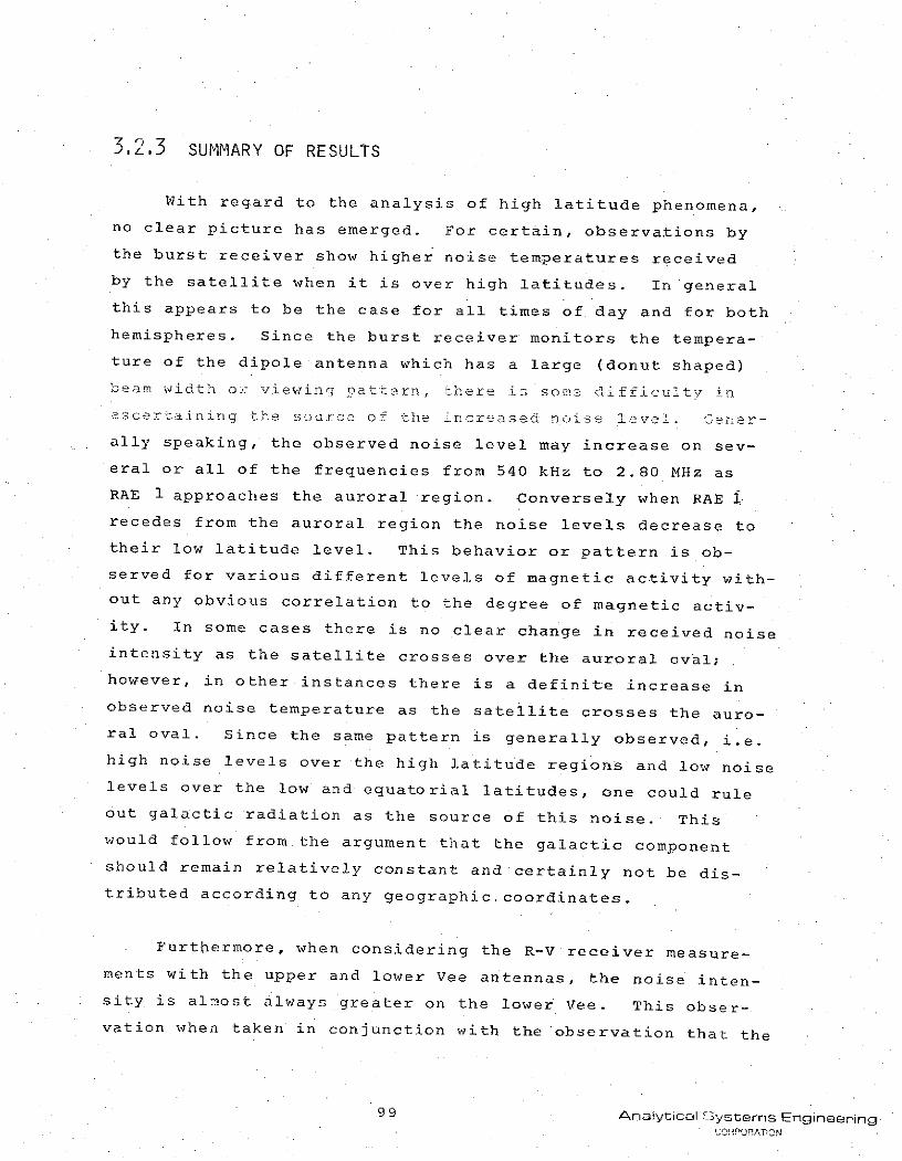
3.2.3 SUMMARY OF RESULTS
With regard to the analysis of high latitude phenomena,
no clear picture has emerged. For certain, observa.tions by
the burst receiver show higher noise temperatures received
by the satellite when it is over high latitudes. In general
this appears to be the case for all times of day and for both
hemispheres. Since the burst receiver monitors the tempera-
ture of the dipole antenna which has a large (donut shaped)
beam width or viewing pattern, there issome di fficulty in
ascertaining the source of the increased noise level. Gen r-
ally speaking, the observed noise level may increase on sev-
eral or all of the frequencies from 540 kHz to 2.80 MHz as
RAE 1 approaches the auroral region. Conversely when RAE 1
recedes from the auroral region the noise levels decrease to
their low latitude level. This behavior or pattern is ob-
served for various different levels of magnetic activity with-
out any obvious correlation to the degree of magnetic activ-
ity. In some cases there is no clear change in received noise
intensity as the satellite crosses over the auroral oval;
however, in other instances there is a definite increase in
observed noise temperature as the satellite crosses the auro-
ral oval. Since the same pattern is generally observed, i.e.
high noise levels over the high latitude regions and low noiselevels over the low and equatorial latitudes, one could rule
out galactic radiation as the source of this noise. This
would follow from the argument that the galactic component
should remain relatively constant and certainly not be dis-tributed according to any geographic.coordinates.
Furthermore, when considering the R-V receiver measure-
ments with the upper and lower Vee antennas, the noise inten-
sity is almost always greater on the lower Vee. This obser-
vation when taken in conjunction with the observation that the
99 Analytical Systems EngineeringCORPORATION
noise intensity at the high frequencies drops off sooner thanit does at lower frequencies leads to the conclusion that the rad-iation emanates from a region below the satellite, but above
the peak of the F 2 -layer. Two further arguments that RAE is
not monitoring ground radiation' are: 1) Radio noise measure-
ments made at ground level indicate that radio noise levels
decrease with increasing latitude and this is not observed
by RAE; 2) Examination of RAE noise measurements during polar
cap absorption and auroral absorption events (the times of
which were supplied by R. Cormiero AFCRL) show no decreasein noise level, which would not be the case if one were ob-
se:ving ground radiation.
Most of the cases examined were for observations made
mainly during the nighttime hours, since the high latitude
geophysical processes of interest are primarily. nighttimephenomena as discussed in Section 3.1. During this time the
F-layer ionization decreases and so also does the lowest pene-
tration frequency thus permitting ground radiation to reach
the satellite. This effect would be further enhanced with
the presence of the high latitude troughs. However, the
measured increase in observed noise temperature most likely
has its origin in the magnetosphere and represents emission
from either precipitating charged particles or electrons trap-
ped in the Earth's magnetic field for the reasons discussed
above. Furthermore, daytime observations that were examined
also reveal a similar pattern of increased noise level at
high latitudes. Particle precipitation does take place on
the day side of the Earth's magnetosphere, even though it is
most intense in the pre-midnight sector. However, because.
of the very sporadic na"ture of the emissions it is not clear
whether the noise intensities are strongest around midnight
magnetic time, as one Tright expect if particle precipitation
were the responsible generation mechanism.
100 Analytical Systems Enginee:ingCO;" ORATION
3,3 RF GENERATION MECHANISMS
3.3,1 SYNCHROTRON RADIATION FROM TRAPPED PARTICLES.
Synchrontron radiation, or the radiation produced by
trapped relativistic electrons spiraling down magnetic field
lines, is important as a possible source of noise. This may
include frequencies from VLF to HF. The objective of this
section is to discuss, in brief outline, the synchrotron
radiiation mecha i sm r as ppiedto a sinle rape eectron,
to ensembles of trapped electrons, and to energetic electrons
trapped in the outer Van Allen belt and precipitating
particles near the auroral zone. The predictions of J.F. Vesecky
are discussed (see Vesecky, 1969) regarding the possibility that
a high latitude satellite may observe 5-20 MHIz synchrotron radiation origin-
ating from magnetospheric regions above the auroral zones.
Finally, the RAE event observed November 3, 1969
from 0310 to 0345 UT is discussed as an example
of possible experimental verification of the prediction. The
sources of information are extracted from articles in the
open published literature and by data provided by RAE. In
addition, the possible role of precipitating auroral electrons
contributing to the RAE measurement is briefly discussed.
SINGLE TRAPPED ELECTRONS
In practice, the synchrotron radiation detected from any
given region of the magnetosphere originates from an ensemble
of particles (electrons being the most important) spiralling
down the field lines. The particles will be distributed in
101Analyt cal Systems Engineering
CORPORATION
energy and also in the initial conditions that determine the
pitch angle which is an important parameter governing the
orbiting particles motion and spatial range. .In any given
magnetospheric region (the outer Van Allen belts for example)
significant temporal variations in particle (electron) density
are observed (Vesecky, 1969). The number of trapped
particles may exhibit, for.example, very large changes during
times of magnetic storms (Williams and Palmer, 1965). The
significance of the large temporal variation in particle
density is that a large temporal variation in radiation may
be expected a> a connseuence. t has been observed that dis-
turbed conditions may increase the trappe particles in rad-
iation belts and also the intensity of auroral particles
precipitating at high latitudes.
The radiation from an ensemble of electrons depends, of
course, on the characteristic radiation from a single par-
ticle, as determined basically by: the particle's energy
(hence, its velocity), the pitch angle of the spiralling
motion, the strength of the magnetic field B , the charge and
mass of the particle and finally, the angle of the observer's
position relative to the plane of the particle's motion.
The dynamics of a charged particle trapped by a magnetic
field is analyzed in many texts. Of importance as regards
radiation emission is the power intensity pattern produced
by the orbiting charge for the cases of non-relativistic
and relativistic electrons.
In the non-relativistic case, the pattern resembles that
of a loop antenna as may be expected. The frequency of rad-
iation is that of the orbiting electron, that is, its gyro
frequency:
Anafytical Sytems EngineeringO: RO5ATION
eBwo o (3-1)
where: = (1_8 2 )
VC (3-2)
The relativistic electrons, however, tend to throw their
energy forward in a narrow beam. An estimate of the beam
width is on the order of:
2m0 c
B.W.T. (3-3)
ee E is the total particle energy. In Figure 3-4.) examples
of patterns as a function of particle energy are shown, where
8, and # are the usual polar and azimuthal angles used to des-
cribe radiation patterns.
=90" 8 0o113=10 01 0 I.v
I. - Z
=90. °
(Wl E: 100 Iv
. .- Z
(d) E 1I0 Mev
Z-
Figure 3-40.Examples of radiation patterns (total power).
103Analytical Systern3 Engineering
CORPORAl O)N
The radiation in the non-relativi-tic case is often
called cyclotron radiation. The relativistic electron's
radiation is called synchrotron radiation. In the non-
relativistic case, the radiation frequency is the orbiting
gyro frequency. In the relativistic case, the observer
views a pulse of radiation occurring at the particle's gyro
frequency.
The Fourier analysis of this wave form then exhibits
the harmonics (or line spectra) of the fundamental gyro
fTeruency. The power spectrum for a r ia tivstic trap)ed
eLecrron has been worked out by many investigators. A
typical and much used example of the synchrotron power
spectrum is given by Panofsky and Phillips as:
e o3n2 tan2 2P (w) e= wrJ F (nS cos) + J (n cosT)1 (3-4)n 82 oR n B 2 n
where: P (T) is the power radiated per unit solid anglenat the angle Y for the nth harmonic.
Wo, g , B are defined in equations (3-1) and (3-2)
y = the angle out of particle's plane of motion
to the observer.
R = radius of curvature which depends on
particle energy E, pitch angle a and Bo
the magnetic field
B = magnetic flux density
n = number of harmonics
The harmonic frequencies are nwo; n = 1, 2, etc.
An expression for the total power radiated by a trapped
relativistic electron in the direction N out of the orbital
plane is given by Peterson and Hower:
104Analytical Systems Engneering
CORPORATiON
2 i Y2 K2 ()P ( =,f) = 3.4X10 a5Rf (1 - +
2) 2[(K ( + +
2 3 (3-5)
.here Y m B+ 2-where . - (1 -B + ? ) (3-6)3
A plot of the above expression for the in plane direction
T=0 at energies in the .128 MeV to 40 MeV is shown in the
Figure 3-41 (Peterson and Hower, 1966).
\ -L
A. A
m b i 7-w 7 th
Figure 3 41. Spectra of single electrons (freqiency).
The magnitude of the B field chosen to estimate th...e power
per electron is 31.8 amp/r : (typical of about 750 km over the
effect on radiation at any other part of the magnetosphere.
!?66) gives an example of adjus.. g the power vs. f curve for
105 Areiytical Systemns Engineerin.-
/:q- [:: _ i! -
'! "-:i''U:: c t 2.: - :~ -F!-:{- : .: -- ;:-- " ,: -:: --::- -.
CORPORTION
28
-t- r r P-
': " r i n:o:dI ' .p... va l....o i... . 4
L ijq t ie I n rg f ,h . r t c . t i
Figure 342 Effect of change in B on the spectrumof A 10 MeV electron.
.t is readily noted from the plotted valus of Figure 3-41
that, at any particular frequency, the more energetic electrons
produce the most intense radiation. At the sae time, at the
lowest frequencies (1-10 MHz) the most energetic electrons
(20-40Figure 32, Effect of change) will produce less radiation than somn e spof the lowertrum
is Itn optimum electron energy and the higher the eplotted fvalues of Figure-
that, at any particular frequency, the morhigher the energy of theeparticle ust be to prons
produce the mossignificant intense radiation. At the sae time, at the
To(20-40 MeV) will produce less radiatio an than semble of elthe lowerns
106 Analytional ystems Engineering
CONSEMBLESOF ELECTRPORATIONCOPORATION
the electron density region whose radiation will be received.
If Pr is the total received power of frequency f from a mag-
netospheric region of volume V, distance r from a receiver,
then:
P P ( ,f EBa2r = II (fE p(E,t,r)dvdEda Watts/m 2 cps2 (3-7)
where: p(Y,f,E,B,a), is the total power of a single electron
and p is the number density of particles of energy E, etc.
The above expression may also include a multiplicative
attenuation term if the propagation :mediun is absorbing.
The two possible mechanisms for absorption are: a medium of
non-zero conductivity lying between receiving antenna and
radiating region when collision frequency and charged particle
density are high enough at the frequency considered; and the-
loss of radiated energy to increase the synchrotron "self-
absorption" motion of electrons. For an auroral case similar
to that of interest, the two have been shown to be insignif-
icant(Vesecky, 1969 ).Obviously, the evaluation of equation (3.-7)
requires considerable knowledge of the radiating region.
Conversely, a measurement of Pr may allow an estimate of a
property of the region such as the number density of particles.
To estimate the possibility of viewing synchrotron radia-
tion from a region (e.g. outer Van Allen belt) along a ray
path traversing the region,requires that the geometry and
particle morphology be modelled sufficiently accurately based
on measured data and suitable semi-empirical or theoretical
models.
Once the morphology of a given region is determined, that
is, the spatial, temporal and energy distribution of particles
(electrons and protons) in a particular region of space so
107Anaiytical Systems Engineering
CORPORATIN
that t]e P(Y,f ,E,Ba) and p(E,U, r) of equation (3-7) can be
evaluated then the received power can beestimated.
Equation (3-7) is then put into a more readily useful form
which allows integration along a ray path from radiating
region to receiver. These may be curved paths if the inter-
vening medium varies systematically in refractive index.
The intervening medium may also scatter or absorb energy.
These effects must be accounted for if of significant mag-
nitude.
Pet-rson ar:d Jower (1i966) have shown ta i is
convenient to express the received power in terms of the
brightness b:
b 2kT= I P(~,f,E,B,a)p(E,U,r)drdEd (3-8)A2
and Vesecky has chosen to re-express equation (3-8)as follows
(see Veseky, 1969):
b = f J(f,s)ds (3-9)
so
where: 00
J(f,s) = f P(f,E,s)N(E)dE (3 10)
0
N(E) is the number density of particles
having an energy lying within E and
E+dE and s represents an arc length
along the propagation path with the
receiver at so.
Given the morphology of a particular radiating medium
traversed by a ray path to a receiver, considerable simpli-
fications can be introduced into the evaluation of b using
equation(3-9), particularly for energetic particles E > .5 MeV.
108 Analytical Systems EngineeringCORPO ATION
Then it is convenient to take a = and T=O as reason-able estimates.
MORPHOLOGY OF PARTICLES AFFECTING RAE
The objective is to examine the possibility of synchro-
tron radiation contributing to or determining the noise re-
ceived when RAE crosses the polar auroral regions. Since the
position of RAE is known as it crosses the polar regions forany particular orbital pass (e.g. Figure 3-9), and alsothe antenna orientation and patern for each frequency i
known, it is possible to determine the possible directions
where received noise must originate. The second directional
bit of information is determined essentially by the direction
of the magnetic field in regions where trapped or precipitatin.g
particles occur together with the expected distribution of
pitch angles. These determine a range of.planes which contain
the direction of particle motion. For synchrotron radiation
most radiation is confined to the planar direction. The amount
of out-of-plane radiation (as determined by the angle Y) dependson the frequency. Finally, by matching up receiver antenna
pattern direction and the directions of planes normal to fieldlines in regions of significant particle density and energy,the receiving rays can be estimated which provide maximum
received radiation. The integration of equation (3-9) then
allows determination of b.
Figure 3-43 shows examples (taken from Peterson and Hower)
of the effect of frequency and electron energy on the single
relativistic electron's beam width as measured approximately
(b) Emn ssion Portern ol Seral Different Ener-)ies
Figure 3-43. Examples of emission patterns.
Some qualitative information regarding two regions that
are candidate sources of synchrotron radiation in the .7 MHz-
9.18 MHz range received by RAE in polar regions is presented in
the following paragraphs,
OUTER BELT AT HIGH LATITUDES
As noted by Hess (1968) measurements by satellites
show that trapped fluxes normally stop fairly abruptly
at some particular latitude .and show a diurnal variation at
high latitudes. Figure 3-44 depicts the latitudinal
extent of stable crapped particles.
110 Analyt2cal Systems Engineering
60 deg 90 deg 60 deg
(no trapping)
trapping5 10
Stabletrapping
30 deg 30 deg
Noon Midnight
60 deg 90 deg 60 deg
Figure 3-44. Calculated locations of the regions of quasitrapping (orpseudo trapping) in the magnetosphere. Particles mirroring inside thoseregions are unable to complete a 180-deg drift around the Earth. Thoseinjected into the left side will be lost into the tail; those injected into theright portion will abandon the magnetosphere through the boundary on the
111
day side [60].
Analytical Systems Engineering
CORPORATION
Figure 3-45 indicates the limit of trapping (in the in-
variant coordinate system) with respect to a normalized flux
J (see Hess, 1968):
100
/10-
I
/I,
0.1 I I r52 54 56 58 60 62 64 66 68
AN, deg
Figure 3-45,Behavior of the upper limit of trapping A, (shown byarrow) before the magnetic storm of April 1 to 2. 1964 (curve a) andduring the main phase of this storm (curve b). The decrease in -Ai is con-sistent with the measured increase in tail field during this storm [531.
112 Analytical Systems EngineeringCO: 'OeFTION
Typical energy spectra for protons and electrons in the
outer belt are presented below (see Hess, 1968). A character-
istic of proton flux is that it is quite stable in time,
whereas electron fluxes are highly variable in time. For both
particles, an exponential model of particle flux as a function
of particle energy is widely used for curve fitting measured
data.
Figure 3-46 gives the value of E relating flux Jo
and energy E by:
- exp -
based on measured data for a range of pitch. angles over L shell
regions L=2 to L-7. Curyes, may be e.xtrapolated to L=10
900 Ratio of proton energy
300 at L to energy at L= 7300,for i and J constant
500-
N N
2000100-
50- ,
2 3 4 5 6 7L
Figure 3-46. Comparison of measured e folding energies Eo from data ofDavis and Williamson [1] with calculated energy variation of protonsduring radial-drift conserving t. and J for various initial pitch angles atL= 7 [6].
113 Analytical Systems EngineerngCOR"O LION
Similarly, Figure 3-47 and Figure3-48 show typic, 1 flux
of energy E electrons over L shells ranging from L=1. 74 to
L=8.20.
107 -1.93 L=2.19=.l112 gauss I=0.120 gauss
0.,=0.07 Mevev106E=.7Mev
S _"-- ~oE=0.10 Mev
5 0. 14 Mev E" 0.091 Mev
L(- = 1.74B B .223 gauss I
0.10 S1 10.0.,.j i-= .," iausV .-t, -- \
0.10 1.0 10.0
E, Mev
107
S10i L =2.65 L= 2.89 L =3.16B=0.131 gauss B=0.135 gauss =0.139 gauss
n=-2.84105 \+
105 -n=-2.77
F--I-
I kf 8 Mev
v 10 -(b)
103
102 B= 0.237 gauss
0.10 1.0 10.0
0.10 1.0 10.0
0.10 1.0 10.0
E, Mev
Figure 3-47. Typical differential electron-energy spectrum measured onSatellite 1964-45a on August 15, 1964. (a) 1.7<L<.2.2. Exponentialdistributions are fitted to the soft component, and an equilibrium fission-data spectrum is fitted to the hard component. The neutron f-decayspectrum is given as a dashed line with the data of L= 1.74. (b) For2.4 < L < 3.2. Power laws are fitted to two sets of data. The data at L =3.16 are fit better by an exponential system. Fission B spectram fitting thehigh-energy points are given as dashed lines.
Analytical Systerms Engineering114 co roi .,roN
107
-_, L 3.49 L=3.91 L=5.04
10 6 =0.13 gauss 1=0.148 gauss I 0.157 gauss
3 ... E, 0.33 MevS105- --
E-,=0.65 Mev
L= 4.9910 n=o.241 gauss
o.52 , ,, -(c)SE=0.52 Mev L=3.93
B=0.241 gauss C
10 B=0.240 gauss
0. ) 1.0 (00.10 1.0 10.0
0.10 1.0 10.0
E, Mev
I I I lI I I i i
107
L=5.91 L 7.06 L=8.20o B=0.162 gauss B=0.166 gauss RB=0.171 gauss
106 ..
0 - -4-.
10 5
0 F L= 5.93P= 0.240 gauss ,= 0 .16 Mev
E= 0.31 Mev
S10 1 - E 0.32 Mev(d)
0
0 103
102
0.10 1.0 10.0
0.10 1.0 10.00.10 1.0 10.0
Figure 3-48. E, Mcv
Tyuical differential electron-energy spectrummeasured on Satellite 1964-45a on August 15, 1974
(c) For 3.4< L 5.0. Exponential spectra fit the data above 0.5 Mev. (d) For 5.9< L < 8.2.
Exponential spectra fit the data given-,.
1 5
Analytical Systems EngineeringC ]RPORATION
An exponential modeling of electron flux J by energy E is
given by equation (3-11)
Diffusion of both protons and electrons is an important
process partially determining spatial and temporal distri-
bution of the particles (see Hess, 1968).
Figure 3-49 provides data and estimates of electron fluxes
in the inner zone (see Hess, 1968).
4
3 -0B
2-D
/ \
0 I -
0 200 400 600 800 1000 1200
Electron energy, Key
Figure 3-49, Various energy spectra of inner-zone electrons. A indicates
the spectrum measured hy Hlolly et al. [41], IB ihe spectrum Imeasred by
Mann et al. [48], (' tlh c alculalted electron spcctrum [52], and I) the spec-
trum measured b Imlmhof it al. [47].
The information in Figures 3-45 through 3-48 yield E, ,
and p which, together with frequency versus energy estimates
of Figure 3-42, allow estimates of brightness b according to
equation (3-8) when the spatial morphology of B and fluxes
are more precisely given.
116
Analytical System:- Engineering
AURORAL PRECIPITATING PARTICLES
It is assumed that the region of precipitating particles
lies within the pseudotrapping region shown in Figure 3-44
It is apparently accepted that most of the particle energy
brought into auroral zones is of energies E < 30 keV, with
the possibility of significant numbers of higher energy also
present. The data of many experiments of energy flux.measure-
ment is summarized in Figure 3-50 (see Hess, 1968) for electrons.
The spectra of protons is probably roughly similar.
108
107 - E'6
106J(> E) electrons
cm-sec
105
10 Eo,-20
10 -
electrons
cm2-sec-Kev ,
10 I I0 50 100 150
Key
Figure 3-50. Typical electron-energy spectra of precipitating auroralelectrons based on various experimental data. Both a differential andenergy spectra are shown. The high-energy region shown as a dotted lineis not vet well known.
117 Analytical Systems EngineeringCORPORATION
Figure 3-51 (see Hess, 1968) in effect provides evidence
that the origin of precipitating auroral electrons is not
primarily from the region of stably trapped electrons and
protons. The rationale is that usually the fluxes of pre-
cipitating and stably trapped particles increase at the same
time, hence, the stably trapped particles are not the immediate and
significant source of precipitating particles.
L, Earth radii
2.0 3.0 4.0 5.0 6.0 7.0 3.0
Injun III Auroral event0705 UT Jan. 31, 1963 and splash
C 106
Electrons E>40 Key '
10 - Electrns E>40 Key
trapped a= 50 deg
N~ light emitted
102
Cleveland, Ohio
0 100 200 300 400 500Time, sec
cI t I 45deg 60deg 65deg 70 deg
Invariant latitude. A
Figure 3 -51Measurements of trapped and precipitated particles and3914 A auroral emission from a pass of the injun ll satellite showing thesimultaneous increases of trapped and precipitating particle fluxes [14.
118Analytical Systems Engineering
CORPORATIONCORPORATION
The direction of synchrotron radiation originating from
precipitating auroral particles will. be in a plane approximately
normal to the magnetic field lines originating in a region about
the auroral oval and projected upward in altitude.
VESECKY'S PREDICTION OF HIGH ALTITUDE RECEPTION OF 5-20 MHz
Vesecky undertook calculation of synchrotron radiation
brightness b according to equations 3-7 , 3-8 ,and 3-9 and a
model of outer belt radiation fluxes of relatively high energy
by Vette. The latter is a codification based on numerous
satellite measurements (see Vesecky, 1969). Figure 3-52 shows
a plan view of an (optimum) region of synchrotron radiation
at an altitude of 4,000 km. Since the most intense radiation
from this region lies in a plane normal to the earth's magnetic
field lines, it may be detected by satellites at higher altitudes.
Vesecky's analysis shows that frequencies in the range 5-20 MHz should
be energetic enough during some disturbed events to be detect-
able above cosmic noise. These frequencies are in the range
observed to be most energetic from the outer belt.
DIPOLE MAGNETIC FIELD LINES
L=5-0
L=40
-8= O12 GAUSS-B=OG16 GAUSS
704
6050,
40'
DIPOLE AXIS 20"
IO 12 14 16 18
MAGNETIC DIPOLE COORDINATE,R-EARTH RADII
Figure 3-52. A VIEW TAKEN .PPEENICUI.AR TO THE DIPOLE AXIS OF A DIPOLE MODEL FOR TIlE GEO-MAGNa Ilc FIEI.D SIIOWING IIIe (R, ;.) COORItINATES OF THE DOMILNANT [MITING REGION.
Ray paths being considered will pass through the enitting region toward the observer whileperpendicular to the plane of the figure.
Analytical Systems EngineeringCORPORAT-ON
119
Figure 3-53 shows levels of cosmic noise brightness and
examples of possible synchrotron noise during disturbed events.
10t-19
ELLIS(1964)GROUND BASED
HARTZ(1964) /ALOUETTE >_
l 20 . /
AURORALCASE- . (100 X AVERAGE FLUX)
PARTHASARATHY* (1966) GROUND 9ASED
S-21 AURORAL CASESD tO X AVERAGE FLUX
u -22 . AURORAL'CASE -m 10 (AVERAGE FLUX)
O ELLIS( 196)b-,GROUND BASED o
\ -----Insy
n
-23 i I -10 10 G 10
7 10
FREQUENCY (Hz)
Figure 3-53 COMPARISON OF SYNCHROTRON EMISSION FROM ABOVE THIE AURORAL REGIONS ( Wy) VITH
SEVERAL ESTIMATES OF THE COSMIC NOISE BACKGROUND (bm).
Figure 3-54 depicts the results of brightness calculations
originating from the region shown in Figure 3-52 for the fre-
quencies 5-20 MHz. For det-ails of these calculations see Vesecky,
1969.
120Analytical Systems Engineering
CORPORATION
Idr
|0.25 _C- I I-MHz
Li ------ l
40 4.2 4-4 46 48 50
L-SHELL
Figure 3-54 ' D)ISTrIitfilON OF OuSERVEFD IRIGHTNESS WITHi TilE REGION IN ([3, L) SPACE FROM WIICH
THE DOMINANT CONTRIIIUTION COMES AT FREQFENCI(S IN THE 50-20 N l[z RANGE: TIHE SOLID)
LINE IMPLIES B , 0.16 G AND THE DASHED LINE 3B 012G.
Finally, it is noted that most of the auroral region
orbital passes during PCA events presented in this report do
support the predictions ofVesecky for the higher end of the
frequency range. Note that the RAE orbit at 6,000 km,which
is above the 4,000 km emitting region shown in Figure 3-52,,
and conditions are approximately those postulated by Vesecky
for detection of 5-20 MHz. Examination of data indicates
enhanced radiation arrives through the lower Vee antenna side
lobes or from below.
Remaining for speculation is the detection of frequencies
well below the 5 MHz lower level predicted using Vette's outer
belt model. It is noted however, that the spectrum of pre-
cipitating particle energy is in the lower energy ranges. Thus,
even though individual electrons at the lower energies provide
little power (see Figure 3-41) the pattern becomes more omni-
directional which fact increases the region and number of par-
ticles whose radiation can contribute. Figure 3-41 also in-
dicates that higher energies up to about 1 MeV contribute to
the radiated frequencies below 1 MHz, but the contributing
regions will be more restricted because of narrow radiation
pattern.
Analytic3l Systems Engineering121 CORPORATION
CONSIDERATIONS CONCERNING SYNCHROTRON RADIATION IN RAE DATA
Analysis of RAE data from PCA events indicate generally that radia-
tion is received on antenna side lobes or from below the satellite. The esti-
mated background shows the upper Vee to be most energetic which
fits the view that cosmic radiation is most efficiently received
from the top Vee. Figure 3-55 shows a plot of upper and lower
Vee background and noise enhancement as the auroral region is
approached. This is the event of November 3, 1969 during which
the subsatellite track entered the oval boundaries. Very
similar looking data occur for passes where the oval is notintersected or even passed very closely. This is still consis-
tent with the picture of synchrotron radiation generated by
precipitating and trapped particles.
It is noted that the RAE.data may provide experimental
information on both large scale and small scale irregularities.
The scattering from small scale irregularities would provide
diffraction patterns that can be relatively narrow or broad as
the spatial separation is many. wavelengths or few. The two
measurements at each frequency (separated by four seconds) in
effect samples the diffraction fine structure.
The RAE data shows a variety of four second interval energy
separations. These can be viewed as the effect of the satellite
passing through the small scale diffraction fringes. It is
possible that a suitable analysis of this data can provide esti-
mates of the statistics of small scale irregularities.
The fine structure is superimposed on large variations of
energy which may be viewed as the effect of the satellite
swinging into the highly directional synchrotron radiation
propagating- through a predominately forward scattering medium
which implies large scale scattering irregularities.
122 Analytical Systems EngineeringCORPORATlON
1010 I I I
5.6 LV MaxEnhanced
Radiation3.2 UV Max
/1.8 t /
o//
5.6 //-
IN PUV Cosmic
\/ Background
8 /10 / LV
5.6- I
..8 -//. /
5.6 -
5.2- \
\/
Nov. 3 1969 0310 - 0345
0 2 4 6 8 0 12
Frequency (MHz)
FIGURE 3-55. NOISE ENHANCEMENTS FOR UPPER AND LOWER VEE FOR 3 NOVEMBER 1969.
123
The rather broad range of frequencies generated and
detected by synchrotron radiation provides a ready made
frequency source over about a decade of frequencies.
124
Analytical Systems ErineeringCORPORATION
3,4 OTHER GEOPHYSICAL AND MAN MADE PHENOMENA
3.4,1 SOUTH ATLANTIC GEOMAGNETIC ANOMALY
Since it is expected that RF emissions from precipitating
particles in the auroral regions will increase RAE noise temp-
eratures, it is reasonable to expect that particle precipi-
tation in other regions of the world will have the same effect.
3,4.2 RF EMISSION DURING ARTIFICIAL AURORA PRODUCTION
In January 1969 a rocket-borne electron accelerator was
launched from Wallops Island for the purpose of creating
detectable artificial auroras (W. Hess, et al., 1971,
T. Davis, et al., 1971). As pointed out in Section 3.3,
precipitating particles may produce RF emissions over a
broad spectrum depending on the particle energies and a
number of other complex factors. The precipitating
particles result.from the natural interplay of the solar
plasma and Earth's magnetic field, or they may be artificially
introduced in a manner similar to therocket -borne particle
generator, or by nuclear detonation.
126Analytical Systems Engineering
CORPORATION
Generally, one can expect that HF emissions may be
produced by accelerating electrons with energies within
the range of those generated during the Wallops Island
rocket launch, i.e. 1 to 10 keV. Consequently, we were
presented with an opportunity to examine RAE data during
the January 1969 experiment, to determine whether there
were any perturbations in the data attributable to enhanced
HF emission generated by the artifically injected electrons.
Detection of the potentially enhanced level of RF
emission required a detailed examination of the RAE data,
the state of the local ionosphere, magnetic and solar
activity information, and prevailing meteorological
conditions. The meteorological conditions are of particular
importance since the rocket was launched shortly after the
passage of a cold front and the atmospheric noise, consisting
primarily of sferics associated with the front,may have been
quite severe. It was our judgement that the results of this.
study would give a further indication of the ability to
differentiate between the many noise generation mechanisms
generally operative near Earth's surface.
As has been the case in the past while investigating
thunderstorm activity, our attempt to observe HF emissions
of artificial aurora has been completely thwarted since RAE
orbits did not traverse the appropriate geographic locale
at those observational times judged critical to the
investigation. Since electrons can remain trapped by the
magnetic field for some time before their energy is
dissipated, additional periods following the time of rocket
launch were investigated. These investigations have failed
to reveal any significant perturbations attributable to
127Analytical Systems Engineering
CORPORATiON
radiation from trapped, artifically injected electrons.
Consequently, due to the unfavorable relation between RAE's
orbital position and the time of electron injection, it is
our judgement that 'it is not possible to arrive at any firm
conclusion regarding enhancements of noise power due to
synchrotron radiation from the injected electrons.
128
Analytical Systems EngineeringCORp'RATON
4,0 CONCLUSIONS
Results of the continuing investigation of RAE I
observations of worldwide terrestrial radio noise and
geophysically significant regions of the Earth have
proved to be very fruitful when viewed in toto. The
fourteen seasonal noise contours based on RAE observations
of HF noise indicate that while there is general agreement,
with.the CCIR predictions regarding the gross character-
istics of terrestrial HF noise, there are many significant
differences. The RAE and CCIR contours begin to diverge
at the higher latitudes, over the Northern Chinese and
Russian mainlands, and frequehtly over ocean regions,
particularly over the North Central Pacific. Large noise
levels at the higher latitudes are attributed to RF
emission processes in the magnetosphere. Differences over
China and Russia are partially attributable to high power
transmitters on the mainland in addition to the lack of
empirical data over this region as evidenced by CCIR. The
lack of ground-based measurements over ocean regions leads one to
believe that the CCIR predictions are suspect over the
oceans. On the other hand, the RAE contours are exclusively
the result of measured data. Overall, the RAE contours
are a valuable contribution to our knowledge of the
noise environment.
Regarding the analysis of high latitude phenomena
no clear picture has emerged. In almost all cases, noise
temperatures are greater at high latitudes than mid-
latitudes for all times of day in both hemispheres. The
fact that the noise temperature is nearly always greater
on the lower Vee coupled with the fact that the noise .temperature at
129 Analytical Systems EngineeringCORPOF ATION
higher frequencies drops off sooner than at lower frequencies
leads one to conclude that the radiation emanates from a region
below the satellite but above the peak of the F 2-layer. This
conclusion is in agreement with the predictions of Vesecky (1969)
A further observation is that noise levels do not decrease
appreciably during polar cap absorption and auroral absorption
events. This behavior is not what would be expected if the rad-
iation emanated from the ground. This observation tends to
reinforce the conclusion-that at high latitudes magnetospheric
Rf en:iL sions enhance noise levels as indicated above.
With regard to known geophysical effects, such. as
the PCA and midlatitude trough, the RAE data do not
reveal their existence clearly as do ground-based riometers
and satellite-borne ion traps. There does not appear to be
a benefit in the RAE data worth the detailed statistical
analysis that would be required to reveal the presence of
the PCA or trough.
There does appear to be a large amount of data available
on the noise generated by precipitating particles in near
space. There is a great deal of variability and structure
in this data when viewed as a function of time, location or
frequency. The meanings and inferences of these RAE data to
the kinds of particles existing in space, their source
and the mechanism of entry into the Earth's magnetic field
have yet to be appreciated.
130 Analytical Systems TngineeringCOPORPOATIC!
RAE measurements of noise levels over the South Atlantic
geomagnetic anomaly have resulted in a number of apparently con-
flicting observations. On the one hand, pronounced high noise
levels are observed on five seasonal contours for Spring, Summer
and Fall for the 0-8 and 16-24 local time blocks on both 6.55 and
9.18 MHz. On the other hand, the remaining 9 seasonal contours
display nothing unusual over this region. Further, the indivi-
dual RAE orbits over the anomaly when compared to control orbits
both east and west of the anomaly show very little differences.
On the basis of the analysis performed to date,, there are no
satisfactory conclusions to be presented. A dceeper understanding
of phenomena observed over the South Atlantic geomagnetic anomaly
requires more extensive analysis and additional independent mea-
surements over the region.
The artifical aurora experiment of January 1969 was not
amenable to analysis since RAE did not traverse the appropriate
geographic region at those observational times judged critical
to the investigation. There was no indication of enhanced noise
due to radiation from trapped artifically injected electrons at
times sometime after the launch. Our judgementis that it was
not possible to arrive at any firm conclusion regarding enhance-
ments of noise power due to synchrotron radiation from the in-
serted electrons.
131 Analytical Systems EngineeringCORPORATION
REFEREN CES
Bailey, D. K., 1964,"Polar-Cap Absorption," Planet, SpaceSci., 1964, Vol. 12.
Bowman, G. G., 1969, ":Ionization Troughs Below the F2-layerMaximum," Planet, Space Sci., Vol, 17.
Carpenter, D. L., 1963, "Whistler Evidence of a '-Knee" in theMagnetospheric Ionization Density Profile," J, Geophys,Res. Vol. 68, No. 6.
Cormier, R., 1974, Private Communication
Chernosky, E. J., 1974, Private Communication
Davis, T.N., T. J. Hallinan, G. D. Mead, J. M. Mead, M. C,Trichel, W. N. Hess, 1971, JGR, Vol 76, No. 25.
Dessler, A. J., Effect of Magnetic Anomaly on ParticleRadiation Trapped in Geomagnetic Field, J, Geophys. Res.Vol. 64, No. 7, 1959.
Herman, J. R., 1972, "High Latitude Spread-F and IonosphericTroughs," Proc. OHD Tech. Review Meeting of 3-4 May 1972,Vol 2, Pg. 149.
Herman, J. R. , J. A. Caruso and R. G. Stone, 1973, "RadioAstronomy Explorer (RAE) I Observations of TerrestrialRadio Noise," Planet, Space. Sci., Vol 21, No. 3.
Hess, W. N., 1968, "The Radiation Belt and Magnetosphere,"Blaisdell.
Jelly, D. H., and L. E. Petrie, 1969, "The High LatitudeIonosphere," Proc. IEEE, Vol. 57, Pg. 1005.
Muldrew, D. G., 1965, "F-Layer Ionization Troughs DeducedFrom Alouette Data," J. Geophys. Res., Vol. 70.
Novaco, James. C., 1973, "Galactic Background Maps at3.93 and 6.55 MHz, Goddard Space Flight Center, ReportNo. X-693-73-182.
Panofsky, and Phillips, 1956, "Classical Electricity andMagnetism," Addison and Wesley.
Peterson, A. M. and G. F. Hower, 1966, "Theoretical Model ofSynochrotron Radiation and Comparison with Observationsof Radiation Trapped in the Earth's Macnetic Field,"(Ed. B. M. McCormack).
13" Analytical Systems EngineeringCORPORATION
Pike, C. P., J. R. Herman and G. J. Gassmann, "ConjugateF-Region Enhancement Related to the South AtlanticMagnetic Anomaly," Radio Sci., Vol. 13, No. 7, 1968,
Reid, G. C., 1963, "A Study of the Enhanced IonizationProduced by Solar Protons During a Polar Cap AbsorptionEvent," J. Geophys, Res,, Vol. 66, No.,12.
Sharp, G. W., 1966, "Midlatitude Trough in the NightIonosphere," J. Geophys. Res., Vol. 71, No. 5.
Vesecky, J. F., 1969, "Radio Frequency SynchrotronRadiation from Trapped Electrons Above the Auroral Zones,"Planet. Space Sci., Vol, 17, pp. 389 to 402.
Weber, R. R.. J. K. Alexander, R. G. Stone, 1971, RadioScience, 6, 1085.
Williams, D. J. and W. F. Palmer, 1965, "Distortion in theRadiation Cavity as Measured by an 1100 km Polar OrbitingSatellite," J, Geophys. Res. 70.
Whalen, J. A., 1970, "Auroral Oval Plotter and NomographFor Determining Corrected Geomagnetic Local Time, Latitude
and Longitude for High. Latitudes in the Northern Hemisphere,"AFCRL-70-0422.