Randomization Metrics: Jointly Assessing Predictability and Efficiency Loss in Covariate Adaptive Randomization Designs Dennis Sweitzer 1 1 Medidata Solutions, 20 Ash Street, Suite 330, Conshohocken, PA 19428 Abstract Randomization methods generally are designed to be both unpredictable and balanced overall and within strata. However, when planning studies, little consideration is given to jointly assessing these characteristics or their impact on analyses. In order to compare randomization performance, we simulated various covariate-adjusted randomization methods (i.e., stratified permuted block, and dynamic allocation), and compared balance and randomness measures both graphically and statistically. We primarily measured predictability by modifying the Blackwell-Hodges potential selection bias in which an observer guesses the next treatment to be one that previously occurred least in a subgroup, reflecting a game theory model of observers versus statistician that is easy to calculate and interpret. We also considered entropy and predictability measures. We primarily measured balance by loss of efficiency using Atkinson’s method, since much of the impact of imbalances within subgroups is lost statistical power and interpretable as lost sample size. We also considered a measure of confounding, and methods of summarizing subgroup imbalances into an overall measure. Key Words: Randomization, covariate, adaptive, dynamic allocation, minimization, selection bias, efficiency loss 1. Introduction Randomization is at the heart of many statistical methods, yet not much research exists comparing the performance of randomization methods and their parameters. We seek distinct & ideally independent attributes of randomization that can be measured by their impact on the statistical analyses. Furthermore, the measurements of attributes must be programmable and should be useful for planning purposes, e.g., if a randomization scheme loses statistical power because of sub-optimal allocation of subjects, it is more useful to express the power loss as the effective number of patients “lost” rather than a change in power (1-ß). The most cited qualities of a good randomization scheme are randomness and balance. Randomness of a schedule is important to minimize allocation bias, selection bias, and to enables blinding of treatment to observers. Allocation bias is essentially a distribution of JSM 2013 - Biopharmaceutical Section 516
Transcript
Randomization Metrics: Jointly Assessing Predictability and Efficiency Loss in Covariate Adaptive Randomization
Designs
Dennis Sweitzer1 1Medidata Solutions, 20 Ash Street, Suite 330, Conshohocken, PA 19428
Abstract Randomization methods generally are designed to be both unpredictable and balanced overall and within strata. However, when planning studies, little consideration is given to jointly assessing these characteristics or their impact on analyses. In order to compare randomization performance, we simulated various covariate-adjusted randomization methods (i.e., stratified permuted block, and dynamic allocation), and compared balance and randomness measures both graphically and statistically. We primarily measured predictability by modifying the Blackwell-Hodges potential selection bias in which an observer guesses the next treatment to be one that previously occurred least in a subgroup, reflecting a game theory model of observers versus statistician that is easy to calculate and interpret. We also considered entropy and predictability measures. We primarily measured balance by loss of efficiency using Atkinson’s method, since much of the impact of imbalances within subgroups is lost statistical power and interpretable as lost sample size. We also considered a measure of confounding, and methods of summarizing subgroup imbalances into an overall measure. Key Words: Randomization, covariate, adaptive, dynamic allocation, minimization, selection bias, efficiency loss
1. Introduction Randomization is at the heart of many statistical methods, yet not much research exists comparing the performance of randomization methods and their parameters. We seek distinct & ideally independent attributes of randomization that can be measured by their impact on the statistical analyses. Furthermore, the measurements of attributes must be programmable and should be useful for planning purposes, e.g., if a randomization scheme loses statistical power because of sub-optimal allocation of subjects, it is more useful to express the power loss as the effective number of patients “lost” rather than a change in power (1-ß). The most cited qualities of a good randomization scheme are randomness and balance. Randomness of a schedule is important to minimize allocation bias, selection bias, and to enables blinding of treatment to observers. Allocation bias is essentially a distribution of
JSM 2013 - Biopharmaceutical Section
516
subjects among treatments such that another factor affects outcomes; since the existence of hidden variables can never be absolutely excluded, random assignment of treatments provides some assurance that a hidden (or known) factors will equally affect all treatment groups. Selection bias implies an observer, who might anticipate the next treatment allocation and adjust his choice of subject accordingly. Blinding of treatment to observers helps ensure that patients in all treatment groups are treated identically regardless of treatment, as well as prevent observers from anticipating the next treatment based on past assignments; Often treatment is not blinded to observers because of study requirements, or accidently (e.g., because of distinct drug side effects); For the purposes of randomization metrics, we assume observers have knowledge of the treatment allocations restricted to subgroups of subjects (e.g., an observer may only know—or guess—treatment assignments at his site). One aspect of randomness to consider is the role of an observer. We define a measure of randomness that is independent of an observer (entropy/syntropy), but whether or not a sequence appears random can depend on the information available to an observer, e.g., a clinician may know the treatment assignments at his own site, but not others: Hence, if the randomization assigns treatments based on allocations at all sites (e.g., non-center specific randomization), a local clinician could not predict the next treatment. Balance between treatments within subgroups is important to avoid confounding of treatment effect with the effects of prognostic covariates, maximize statistical efficiency, and provide face validity. For example, if drug & placebo were dispensed in a clinical trial so that most women received the drug, and most men received placebo, the effects of drug and sex could not be distinguished, the variance of the treatment estimate would be larger (reducing statistical power), and could result in misleading implications (e.g., that the drug causes elevated prolactin levels). We focus on the attributes of confounding and efficiency to assess treatment imbalances as it could affect the results of later analysis in causing bias (due to confounding) and increasing variability of the treatment estimate (due to loss of efficiency). However, it is often the case that the target treatment balance for a study is not optimal for efficiency or confounding by design. In that case, we propose a metric that behaves like loss of efficiency in the case of equal treatment allocations, in that it is highly correlated with that measure. Use of randomization metrics such as those proposed here would allow comparisons of randomization methods and their parameters when planning a study by simulating the expected patient population and covariate factors, and applying these methods to the simulations. Conditions which would affect the choice of a randomization methods would include study size, whether it is blinded, the number of covariates, the expected sizes of subject subgroups, subject discontinuations, etc.
JSM 2013 - Biopharmaceutical Section
517
2 Simulation 2.1 Outline of Simulation Using R, we simulated 500 studies of 200 subjects each. All randomization methods were applied to the same set of subjects in each simulated trial, allowing direct comparisons between methods (such as correlations). Randomization metrics were applied after 25, 50, 100 and 200 simulated subject in each study, allowing us to make comparisons of performance between interim analyses. 2.3 Stratification Factors used in Simulation Typically, clinical trials use a small number of covariates to stratify the randomization, plus sites, so we used covariates with 2, 3, and 10 levels, and for convenience denoted them as: Sex, Age Group, and Site/Variant. When the 10 level factor is referred to as a site, it denote information that is known to an observer (along with Sex and Age), while if it is referred to as a variant (like a genetic variation), it denotes information that is not known by observers. Most simulations in the literature make the convenient assumption that stratification factors define equal sized groups, however, clinical trial experience is that equal sized stratification factors are uncommon. Sites in particular show are large variation in sizes. For convenience, we assume that the proportion of subjects in each factor group follows a Zipf-Mandelbrot distribution, in which the probability of a subject belonging to the kth largest level of a stratification factor is proportional to the inverse of a power of k. (Equation 1)
The Zipf-Mandelbrot distribution is observed in many contexts, such as the frequency of words in a language, sizes of cities, abundance of species in an ecosystem, and numbers of visits to websites, and seems to arise when entities compete for limited resources, new entities can be created, and old entities can merge. While sizes of sites might be more accurately modeled assuming a gamma distribution (Anisimov, 2009), this distribution is primarily chosen for convenience & generality: Small subgroups have the largest impact on analyses in clinical trials, and both distributions yield a disproportionate number of small subgroups; The default parameters of k=0 and a=1 yield a reasonable distribution of subgroup sizes for any number of subgroups, while a gamma distribution requires the specification of two parameters (shape and scale/rate/mean). The following table shows the sizes of covariate subgroups used in our simulations, using default Zipf-Mandelbrot parameters of k=0 and a=1
pk ∝1
k + c( )a
JSM 2013 - Biopharmaceutical Section
518
Table 1. Distribution of Stratification Factors
Sex (2:1)
Age Group (1:½:⅓ )
Female Male 67% 33%
Mid. Aged 55% 36% ♀, M 18% ♂, M Young 27% 18% ♀, Y 9% ♂, Y Older 18% 12% ♀, O 6% ♂, O
Site / Variant a B c d e f g h i j Share 34% 17% 11% 8.5% 6.8% 5.7% 4.9% 4.3% 3.8% 3.4% Expected size in simulating:
2.2 Analysis Model The simulation model assumes that the data from the simulated trials will be analyzed using an ordinary ANCOVA model of: (Equation 2)
Outcome = Treatment + Sex + Age + Sex*Age + Variant/site+ error The model can be rewritten in matrix form for use in calculations as: (Equation 3)
E(Y) = zα + Xβ In which: z is a vector of treatment assignments. For convenience in calculations with 2 treatment choices, zj = +1 if subject is one the 1st treatment; otherwise zj = -1 X is the design matrix, in which rows correspond to subjects and columns to covariates α is the treatment effect β is the vector of covariate effects. Since the covariates in this model are discrete and finite, the subjects are members of a collection of overlapping covariate subgroups (e.g., all males, all females, all young people, all young males, etc), and it will be convenient to refer to them as such in some definitions of randomization metrics. Since they are defined strictly in terms of covariates using in the statistical model, they are distinct from the subgroups defined as randomization stratification factors (which typically will be a subset of the covariate subgroups – see Table 3).
JSM 2013 - Biopharmaceutical Section
519
3. Attributes and Proposed Measures When presenting results, generally measures of randomness will be presented on the vertical axis, and measures of balance will be on the horizontal axis. Metrics will be transformed so that the origin corresponds to the theoretically ideal randomization (i.e, if y=0, it cannot be more random, and if x=0, it is in perfect balance and cannot be more efficient or less confounded) Metrics are summarized over simulations as the mean values with an 80% confidence interval defined by the 10th and 90th percentiles.
Figure 1. Venn Diagrams of Randomization Metrics 3.1 Randomness 3.1.1 Predictability/Potential Selection Bias Predictability is defined as potential selection bias in relation to an observer: How well can an observer guess the next treatment, given their knowledge of the state of the randomization system? In a study, typically an observer will only know the stratification factors for the patients enrolled at their site; Consequentially, if past treatment assignments are known, it maybe possible to judiciously guess at the next treatment and increase the odds of being correct. An analogue would be multiple choice tests: if a test taker can eliminate one or more choices, they can increase their scores substantially; In college admission tests (like the SAT), even a relatively small change can make the difference between acceptance or rejection by a school. We use a Blackwell-Hodges (1957) type guessing rule to measure the potential section bias. This frames the problem as a guessing game between statistician and observer in which the observer scores a point for every correct guess, and the statistician’s goal is to limit the score to no better than chance. Since incorrect guesses can be as informative in a
Randomness
Predictability (by observer)
Entropy (no observer)
Periodicity (patterns)
⟶
Y (as a function of probabilities)
Balance
Efficiency (Variability)
Confounding (Bias)
Deviation from Target (Convenience)
X (as # or % of subjects) ⟶
JSM 2013 - Biopharmaceutical Section
520
clinical trial as correct guesses (e.g., if observers expect patients to improve on a drug, but they actually get worse, they may identify treatment groups, though not specific treatments). (Equation 4)
Score = | %Correct - Expected (%Correct) | The Blackwell-Hodges approach is for the observer to always guess that the next treatment will be the one that best restores the target treatment allocation. In order to calculate this score, treatment allocations are tracked for every subgroup of subjects defined by stratification factors (and combinations thereof: e.g., a young male subject would contribute to the cumulative treatment allocations within the group of young subjects, within males, and within young males). If the observer’s knowledge is restricted to the treatment allocations in mutually exclusive subgroups of subjects (defined by factor levels), the score from a treatment assignment is based only on the treatment balance within the subgroup to which the subject belongs, and the potential selection bias for the simulated study is a simple sum over the subgroups. If the observer’s knowledge includes treatment balances from overlapping subgroups, a potential selection bias score is kept for each subgroup (defined by factor levels), and the potential selection bias is the maximum potential selection bias among the subgroups to which the subject belongs. 3.1.2 Periodicity The above definition of predictability only measures the average rate of success, and does not consider any predictable patterns within the randomization sequence. An example of a periodic pattern occurs within permuted block randomizations, whereas the last treatment assignment within a block is completely determined by the previous treatment assignments within the block. We measure periodicity in an ad hoc way analogous to a discrete fast Fourier transform, however applied to the maximum probability among the set of treatment at the time a subject is randomized. In a randomization scheme for subjects j, let (pA,j, pB,j, …) be the probabilities of assigning patient j to the respective treatment A, B, , etc., at the time that subject j was randomized. Then the set of treatment assignments within a subgroup G of patients is denoted by the a of probability vectors (Equation 5), and the list pMax (Equation 6) is the list of maximum assignment probabilities. (Equation 5)
𝒑𝑨,𝒋,𝒑𝑩,𝒋,… ,𝒑𝑪,𝒋, 𝒋∈𝑮
(Equation 6)
JSM 2013 - Biopharmaceutical Section
521
𝒑𝑴𝒂𝒙,𝒋 𝒋∈𝑮= 𝑴𝒂𝒙 𝒑𝑨,𝒋,𝒑𝑩,𝒋,… ,𝒑𝑪,𝒋
𝒋∈𝑮
For the periodic pattern found in permuted block of size k, the last probability in a block, will be 1 for one treatment (and 0 for the others), hence pMax,k*i =1. The algorithm scans for repeating peaks in pMax by averaging every (k*i +j)th value of pMax for j=0…(k-1), resulting in a triangular array of average pMax’s. (in which the row k is the block size, and the column j is the element within a block). The overall average of pMax is subtracted from each element, resulting in an average “excess probability” qk,j for position j within blocks of length k (j=1 to n) (Table 2).
Table 2. Pattern Matrix for Periodicity
Blocks of length: 1st in k 2nd in k 3rd in k ….etc kth of k
k=8 qk,1 qk,2 qk,3 … qk,k For each simulation iteration, periodicity pattern matrices are computed for every subject subgroup of interest, and then averaged between simulations (within each subgroup) to provide a measure of periodicity observed within each subgroup. The overall measure of periodicity is the maximum average periodicity among the subgroups. Consequently, the measure of periodicity is essentially the maximum amplitude of the probabilities in a repeating pattern. The length of the pattern and offset of the peak is available from the algorithm, but is not pertinent to this paper. Because of the limited size of simulated studies, few subgroups are large enough to reliably calculate periodicity for longer patterns (we take twice the length of the longest repeating pattern as the minimum size of a patient subgroup to be analyzed), hence the point estimate of periodicity is the average over all simulations. Using pMax this way reveals periodic causal patterns (in which a sequence of assignments forces a treatment assignment, such as in permuted block randomization). Modifying the same algorithm using the assignment probabilities for each treatment {pA,1, pA,2, pA,3,…}, {pB,1, pB,2,…}, etc. instead of {pMax,1, pMax,2, pMax,3,…}, should also reveal regular patterns for each treatment. However, it should be noted that this approach best identifies treatment probabilities that are periodically large; treatment probabilities that are usually large contribute more to the predictability measure. 3.1.3 Entropy/Syntropy The above predictability and periodicity measures are complicated by the necessary assumptions on the knowledge of an observer. Hence we also want a randomness measure that eliminates the implied observer and provides a measure of intrinsic
JSM 2013 - Biopharmaceutical Section
522
randomness of the system, i.e., if an observer knows the algorithm and the status of the system, how much randomness is left in the system? We define a measure of determinism and call it syntropy (a term first used by Buckminster Fuller as the opposite of entropy), and calculate it as: (Equation 7)
𝑆𝑦𝑛𝑡𝑟𝑜𝑝𝑦 = 1 − log (𝑝!)
!!!!
𝐽 ∗ log (#𝑇)
where J is the number of subjects, #T is the number of treatments, and pj is the probability of selecting the treatment that was assigned to subject j, at the time of randomization. In the notation of (Equation 5, if subject j=8 is assigned to treatment B, p8 = pB,8. This is exactly the Self Information Content -Σlog(pj) (Roman, 1992) averaged over the number of subjects and rescaled to the interval [0,1] so that syntropy=0 represents maximum randomness, and 1 indicates maximum determinism. While syntropy can be calculated for each covariate subgroup, we use the total syntropy for all subjects. If target treatment allocations are not equally distributed, under this definition, syntropy>0, and if less frequent treatments are over-represented in a randomization schedule, it is possible that syntropy<0. 3.2 Balance 3.2.1 Loss of Efficiency We use Atikinson’s (2003) definition of Loss of Efficiency. Using the notation of (Equation 3), the variability of the estimated treatment effect (α) is given by:
The Loss of Efficiency (LOE) below expresses a penalty in number of subjects against statistical efficiency (NB: ztz is the number of subjects). Note also that the above equation clearly shows LOE to only affect the variability of treatment effect. Equation 8.
3.2.2 Confounding For this paper, we defined an ad hoc, simplistic and intuitive definition of a confounding score as the total number of subjects in stratification subgroups in which all subjects are assigned to a single treatment. E.g., if 5 young male subjects are all on the same treatment, they add 5 points to the score; If also 2 young female subjects are all on the same treatment, they add 2 points to the score; Furthermore, if all young people are on
Var(α̂) = σ 2
ztz− ztX(XtX)−1Xtz
LOE = ztX(XtX)−1Xtz
JSM 2013 - Biopharmaceutical Section
523
the same treatment, they contribute another 7=5+2 points to the score (but if young males and young females are on different treatments, the confounding score for young people is 0). 3.2.3 Weighted Deviance Balance in a randomization scheme is often defined in an ad hoc & intuitive way without consideration of the effects on the analysis of the imbalances within the randomization stratification factors, e.g., perhaps the maximum or average percent imbalance observed between randomization strata. Since a target treatment allocation might not be chosen for best efficiency and least confounding, one cannot measure the effect of imbalances using efficiency & confounding. We considered several formulas for summarizing the imbalances across covariate subgroups as weighted combinations of subgroup imbalances, and compared them empirically using correlation with LOE. Consequently, the weighed deviance can be treated as a proxy for LOE when the target treatment allocation is not equiprobable. We considered 3 measures of imbalance of a treatment within a subgroup: (1) The difference between the count of subjects assigned to that treatment and the expected number (in the subgroup); (2) the difference between the percent of subjects assigned to that treatment and the target treatment allocation; (3) the weighted deviance, as the percent difference times the square root of the subgroups size. Within each covariate subgroup, the absolute values of these were summed over the treatments. We considered 3 formulas for summarizing imbalance between subgroups: (1) The mean; (2) The maximum; (3) The Root Mean Square (RMS), defined as the square root of the sum of squares. The RMS is typically used to take the “sum” of standard deviations (since the variance of the sum of a set of random variables is the sum of the variances of each of the random variables). 3.3 Randomization Methods Tested All metrics were tested by using simulations assuming a 1:1 treatment allocation. Complete (or Simple) Randomization (denoted CR) always assigns treatments using the same treatment allocation (no modifications for previous treatment imbalances) In the following figures and table, Stratified Permuted Block (PB, or SPB) randomization is denoted by the prefix “pb”, followed by the treatment allocation. In these, each strata (i.e., sex and age group) is essentially allocated a sequence of permuted treatment blocks from which assignments are made. Stratified permuted block only aims to maintain balance within each strata and if imbalances usually occur if a strata does not contain complete blocks (if block size = 4, and 7 subjects have been allocated to a group, it will be imbalanced). Hence marginal imbalances (which are unions of strata, e.g., all males, all young, etc) tend to become imbalanced. Lebowitz’s (2012) version of Dynamic Allocation (DA) is denoted by the prefix “da”, followed by a letter indicating the stratification subgroups, and the 2nd best probability parameter (this adds an element of randomness to the algorithm). In Dynamic Allocation, imbalances within subgroups are calculated for each treatment arm, as if the subject were
JSM 2013 - Biopharmaceutical Section
524
assigned to that treatment arm. (Imbalances are measured as a percent of the subgroup.) The subgroup imbalances are combined as a weighted sum within each treatment arms, and the treatment assignment that will result in the best balance (indicated by the weighted sum) is preferentially chosen (if there is a tie, each of the tied treatment arms are equally likely to be chosen). If the 2nd best probability= φ > 0, then if there are no ties, the treatment arm resulting in the 2nd best balance is chosen with probability φ. If φ=0, only the treatments arm(s) which best restore balance are chosen. One advantage DA has over SPB in that it attempts to correct marginal imbalances, and factor weights can be chosen to prioritize balance within some factors. Another is that it can attempt to balance on large numbers of covariates. However, DA is often perceived as more deterministic than SPB, hence is often only used when it has compelling advantages. However, the metrics in this paper can be used to compare methods for specific situations and parameters. The randomization methods were tested with different sets of randomization stratification factors and notations in Table 1. PB was simulated using 1:1, 2:2, 3:3, 4:4, 6:6 and 8:8 blocks, and DA using 2nd best probabilities of 0%, 10%, 20%, 30%, and 40%. All factor weights were taken to be 1. The DAD factors (with a weight of 1) are probably the most commonly used as a default when DA is implemented. Table 3. Covariates and Stratification Factors in Randomization Methods Analysis Model Prognostic Covariates
Outcome= Sex + Age + Sex*Age + Site/Variant
Randomization Method Stratification Factors
pb
Sex*Age daE Sex + Age + Sex*Age daM Sex + Age
daS
Sex*Age daC Sex + Age +
Site/Variant
daD Sex + Age + Sex*Age + Site/Variant
4. Results
4.1 Deviation from Target Allocation The weighted deviance imbalance measure (within subgroups), summarized between subgroups with the RMS formula showed the greatest correlation with the LOE (Table 4) with ρ =0.95, at 200 subjects, and ρ=0.89 at 50 subjects. Average and RMS of the percent imbalance performed almost as well, at ρ=0.92. DA usually uses a weighted average of percent imbalances within subgroups to help determine the next treatment assignment, which showed a high correlation with LOE
JSM 2013 - Biopharmaceutical Section
525
Table 4. Correlation between LOE and Deviance Measures
Summation Formula
200 Subjects
Imbalance Measure Maximum Average RMS
Count c 0.72 0.73 0.77
Percent p=c/n 0.78 0.92 0.92
Weighted c/√n = p*√n 0.89 0.87 0.95
50 Subjects
Count c 0.59 0.66 0.66
Percent p=c/n 0.39 0.83 0.79
Weighted c/√n = p*√n 0.79 0.81 0.89
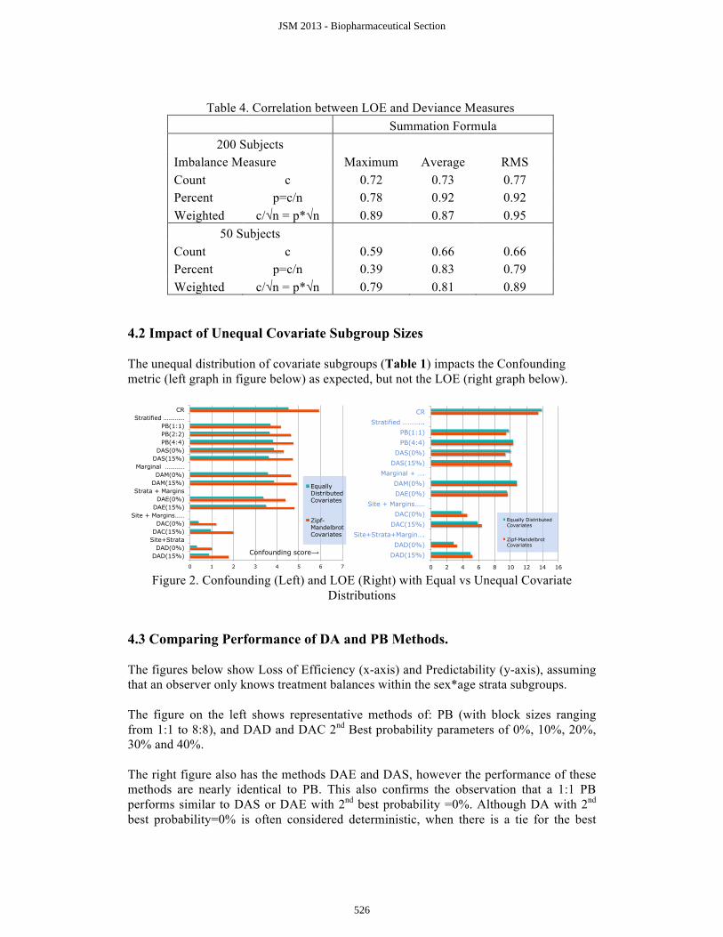
4.2 Impact of Unequal Covariate Subgroup Sizes The unequal distribution of covariate subgroups (Table 1) impacts the Confounding metric (left graph in figure below) as expected, but not the LOE (right graph below).
Figure 2. Confounding (Left) and LOE (Right) with Equal vs Unequal Covariate
Distributions
4.3 Comparing Performance of DA and PB Methods. The figures below show Loss of Efficiency (x-axis) and Predictability (y-axis), assuming that an observer only knows treatment balances within the sex*age strata subgroups. The figure on the left shows representative methods of: PB (with block sizes ranging from 1:1 to 8:8), and DAD and DAC 2nd Best probability parameters of 0%, 10%, 20%, 30% and 40%. The right figure also has the methods DAE and DAS, however the performance of these methods are nearly identical to PB. This also confirms the observation that a 1:1 PB performs similar to DAS or DAE with 2nd best probability =0%. Although DA with 2nd best probability=0% is often considered deterministic, when there is a tie for the best
0 1 2 3 4 5 6 7
CR Stratified ………...
PB(1:1) PB(2:2) PB(4:4)
DAS(0%) DAS(15%)
Marginal ………… DAM(0%)
DAM(15%) Strata + Margins
DAE(0%) DAE(15%)
Site + Margins…… DAC(0%)
DAC(15%) Site+Strata
DAD(0%) DAD(15%)
Equally Distributed Covariates
Zipf-Mandelbrot Covariates
Confounding score⟶
0 2 4 6 8 10 12 14 16
CR Stratified ………...
PB(1:1) PB(4:4)
DAS(0%) DAS(15%)
Marginal + …. DAM(0%) DAE(0%)
Site + Margins…… DAC(0%)
DAC(15%) Site+Strata+Margin….
DAD(0%) DAD(15%)
Loss of Efficiency (LOE) ⟶
Equally Distributed Covariates
Zipf-Mandelbrot Covariates
JSM 2013 - Biopharmaceutical Section
526
treatment to allocate, it choses equi-probably, much the same as treatment assignments using a 1:1 PB. The common element between these 3 methods is that they have the sex*age stratification factor in common, without using site, as a stratification factor. Since the sex*age strata are the smallest stratification subgroups, a 1 subject difference in treatments yields the largest change in %imbalance within strata (because the denominators are smaller). Consequently, these randomizations are dominated by imbalances within strata.
Figure 3. Predictability vs LOE assuming observer only knows treatments in strata subgroups, with n=50. Left is PB, daD, and daC methods, Right adds daE and daS.
4.4 Flexibility of DA for Changing Circumstances. The figures below redefine predictability to limit the knowledge of the observer to the treatment allocation within sites. On the left are the same representative methods as previously; methods that do not use site as a stratification factor become unpredictable (PB, DAE, DAS), while methods that do use site become more predictable the fewer other factors they use. In the DA algorithm, weights of stratification factors can be adjusted to chance performance. The figure on the right shows the changes in performance as the weight of the site factor is set to: 1 (daD), 0.75 (daD8E), 0.5 (daD5E), 0.25 (daD3E), and 0 (daE).
JSM 2013 - Biopharmaceutical Section
527
Figure 4. Predictability vs LOE assuming observer only knows treatments in marginal subgroups (n=50). Left is PB, daC, daD; Right adjusts weight of site factor (note the enlarged vertical scale).
4.5 Syntropy and Periodicity. The figure below on the left plots syntropy versus LOE. DA methods that include many stratification factors seem to become more deterministic because the more factors that are used to calculate weights, the fewer imbalance ties occur. The figure below on the right plots Periodicity versus LOE. PB actually shows a stronger periodicity as block size increases, while it weakens in DA as the 2nd Best Probability increases.
Figure 5. Syntropy and Periodicity vs. LOE
JSM 2013 - Biopharmaceutical Section
528
4.6 Increasing Sample Size. The following figure shows the effect on performance as sample size increases (in the figure, the larges symbols are for simulations of 200 subjects, the smallest, 25). PB increases predictability and slight increases efficiency in going from 25 to 200 subjects; DAD substantially improves LOE with little change in predictability; DAC improves in both LOE and Predictability. The last figure shows the performance of the DA algorithm described by Kuznetsova & Tymofyeyev (2012) with 2nd Best Probability =0, and for 4 sets of stratification factors.
Figure 6. Changes in Predictability and LOE with Increasing Size. Top Left: PB; Top Right: DAD; Bottom Left, DAC; Bottom Right, Kuznetsova 2012 DA with various factors.
JSM 2013 - Biopharmaceutical Section
529
5. Discussion We have proposed and demonstrated a set of attributes and corresponding metrics for evaluating and comparing randomization methods and choices of parameters within expected subject populations. The simulation results here provide some insights into optimizing the performance of randomization methods, such as choice of factor weightings (e.g., reduce the weights for factors within which observers might know treatment assignments), choices of parameters (e.g., DA with 2nd best probability = 0.20 performs similarly to a 3:3 PB), or possible changes to algorithms that might improve performance (e.g., use of the root-mean-squares instead of averages to summarize overall treatment imbalance). These results also demonstrate the possible value of using these methods in planning some studies to evaluate choices of algorithms and parameters in regards to the expected subject populations (e.g., numbers of factors and sizes of stratification subgroups), and study design (e.g., blinding, expected knowledge of investigators, etc).
References Anisimov, V. 2009. Predictive Modelling of Recruitment and Drug Supply in Multicenter
Clinical Trials. In JSM Proceedings, Biopharmaceutical Section. Alexandria, VA: American Statistical Association. 1248-1259
Atkinson, AC. (2003) The distribution of loss in two-treatment biased-coin designs. Biostatistics, 2003, 4, 2, pp. 179–193
Blackwell, D. and J.Hodges Jr (1957). Design for the control of selection bias. Ann Math Stat 28, 449-460
Kuznetsova, O, and Tymofyeyev, Y. (2012) Preserving the allocation ratio at every allocation with biased coin randomization and minimization in studies with unequal allocation. Statistics in Medicine, 2012, 31 701-723
Lebowitsch, J, et al, (2012). Generalized multidimensional dynamic allocation method. Statistics in Medicine, 2012;
Roman, S. (1992). Coding and Information Theory. New York: Springer-Verlag. Print. Wikipedia contributors. "Entropy (information theory)." Wikipedia, The Free
Encyclopedia. Wikipedia, The Free Encyclopedia, 23 Apr. 2013. Web. 14 May 2013. Wikipedia contributors. "Zipf’s Law." Wikipedia, The Free Encyclopedia. Wikipedia,
The Free Encyclopedia, 25 July 2013. Web. 3 August 2013.