Proactive vehicle re-routing strategies for congestion

avoidanceJuan (Susan) Pan*, Mohammad A. Khan*, Iulian Sandu

Popa+, Karine Zeitouni+ and Cristian Borcea* *New Jersey Institute of Technology, USA

+University of Versailles Saint-Quentin-en-Yvelines, France

DCOSS 2012

2

Traffic congestion: an ever-increasing problem

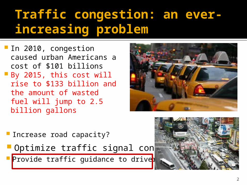
In 2010, congestion caused urban Americans a cost of $101 billions

By 2015, this cost will rise to $133 billion and the amount of wasted fuel will jump to 2.5 billion gallons

Increase road capacity?

Optimize traffic signal control? Provide traffic guidance to drivers?

3

Congestion avoidance using mobile sensing and actuation (1)

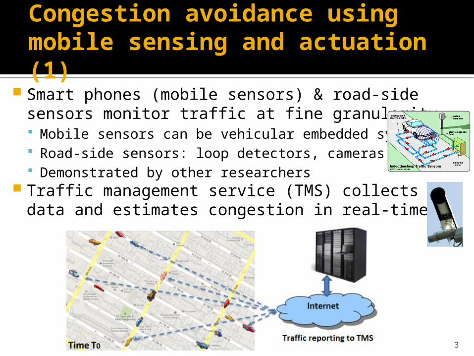
Smart phones (mobile sensors) & road-side sensors monitor traffic at fine granularity Mobile sensors can be vehicular embedded systems Road-side sensors: loop detectors, cameras, etc Demonstrated by other researchers

Traffic management service (TMS) collects data and estimates congestion in real-time

4

Congestion avoidance using mobile sensing and actuation (2)

TMS provides real-time, proactive, individually-tailored re-routing guidance to drivers to prevent congestion Drivers provide their origin-destination

information Guidance is pushed to drivers’ smart phones

when signs of congestion are observed on their current route

Drivers may or may not follow the guidance The main focus of our research

5

Comparison with existing work (1)

Google, Microsoft & Inrix: real

time traffic info to compute

traffic-aware shortest routes Reactively provide same

guidance for all drivers

Problem: move congestion from

one spot to another▪ Similar to route oscillation in

computer networks

6

Comparison with existing work (2)

Transportation researchers proposed dynamic traffic assignment models Iteratively calculate shortest paths and assign

routes to each driver to achieve the user/system equilibrium

Example of systems: DynaMIT, Contram Problems ▪ Tractability at scale (providing real-time guidance)▪ Ability to work when not all drivers are part of the

system▪ Robustness to drivers who ignore the guidance

7

Outline

Motivation & related work

Our 3 proactive re-routing strategies

Simulation results

Conclusion and future work

8

The 4 phases of re-routing

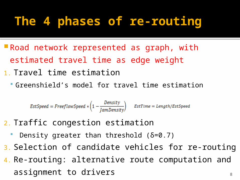
Road network represented as graph, with estimated

travel time as edge weight

1. Travel time estimation Greenshield’s model for travel time estimation

2. Traffic congestion estimation Density greater than threshold (δ=0.7)

3. Selection of candidate vehicles for re-routing

4. Re-routing: alternative route computation and

assignment to drivers

9

Selection of candidate vehicles for re-routing

Step 1: Detect road segments with signs of congestion

Blue: 1st level incoming segments

Green: 2nd level incoming segments

Step 2: Recursively select incoming segments to “congested” segment until depth L

Step3: Select vehicles on these road segments

10

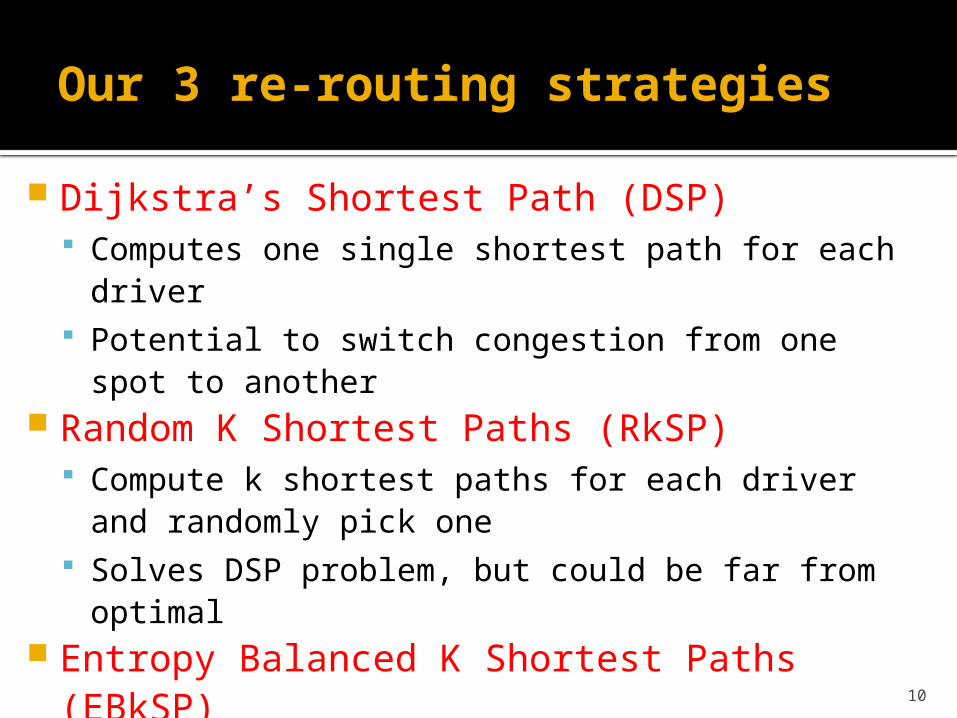
Our 3 re-routing strategies

Dijkstra’s Shortest Path (DSP) Computes one single shortest path for each driver Potential to switch congestion from one spot to

another Random K Shortest Paths (RkSP)

Compute k shortest paths for each driver and randomly pick one

Solves DSP problem, but could be far from optimal Entropy Balanced K Shortest Paths (EBkSP)

Prioritize candidate vehicles Compute k shortest paths for each driver and pick

the one with least popularity Improves on RkSP by choosing better paths

11

EBkSP popularity entropy

Let (p1,…, pk) be the set of k paths that will be assign next

Let (r1,…, rn) be the union of all segments of (p1,…, pk), and (fc1,…,fcn) be the set of weighted footprint counters

Def: Entropy(pj) is the entropy of pj and is computed as

Def:

Def: the weighted footprint counter fci of a road segment i is: fci =ni х wi ni is the number of vehicles that are assigned to paths that include this segment, and wi is the weight of the road segment

12

EBkSP example

a b c d e

f g h i j

k

V2, assigned path (fg, gh, hi, ij )V1, assigned path (ab, bg,gh, hi, ij )V3, assigned path (ch, hk )P1 (ab, bg, gh, hi, ij) fc(P1)(1,1,2,2,2) entropy=1.49P2 (ab, bc, ch, hi, ij) fc(P2)(1,0,1,2,2) entropy=1.16P3 (ab, bc, cd, di, ij) fc(P3)(1,0,0,0,2) entropy=0.58

?

13

Evaluation

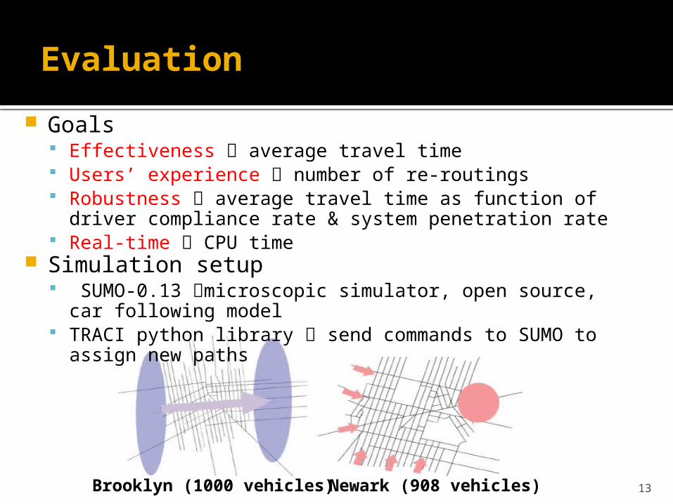
Goals Effectiveness average travel time Users’ experience number of re-routings Robustness average travel time as function of driver

compliance rate & system penetration rate Real-time CPU time

Simulation setup SUMO-0.13 microscopic simulator, open source, car

following model TRACI python library send commands to SUMO to assign

new paths

Brooklyn (1000 vehicles)Newark (908 vehicles)

14

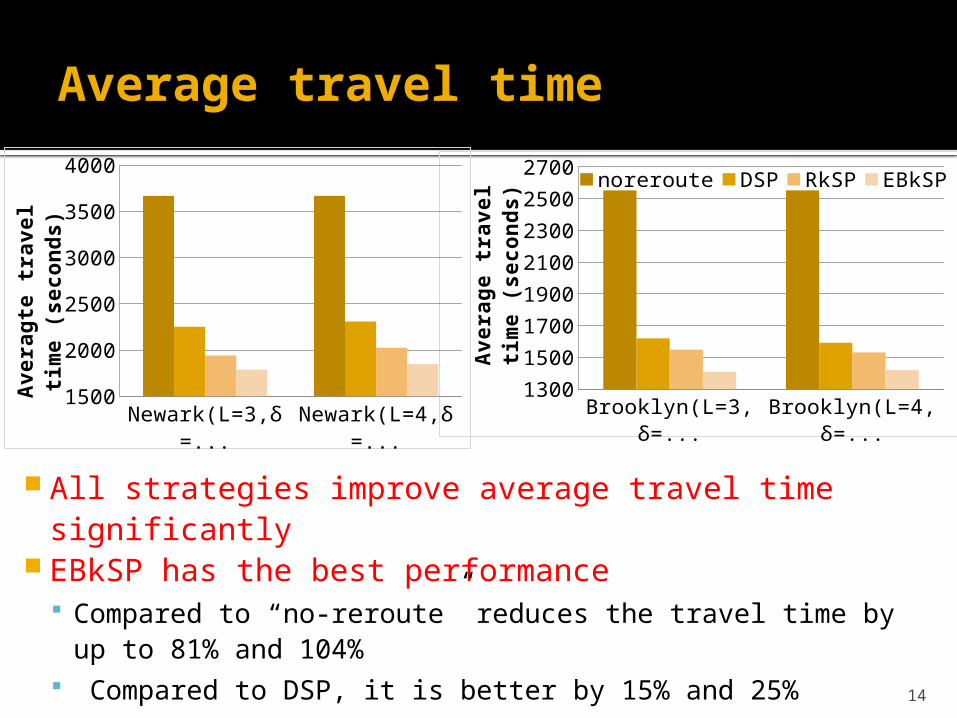
Average travel time

All strategies improve average travel time significantly EBkSP has the best performance

Compared to “no-reroute” reduces the travel time by up to 81% and 104%

Compared to DSP, it is better by 15% and 25%

Brooklyn(L=3,δ=0.7)

Brooklyn(L=4,δ=0.7)

1300

1500

1700

1900

2100

2300

2500

2700 noreroute DSP RkSP EBkSP

Avera

ge t

ravel

tim

e (

seco

nd

s)

Newark(L=3,δ=0.9)

Newark(L=4,δ=0.9)

1500

2000

2500

3000

3500

4000

Avera

gte

tra

vel

tim

e (

seco

nd

s)

15

Average number of re-routings

EBkSP has least number of re-routings Less distraction to drivers

Newark(L=3,δ=0.9)

Newark(L=4,δ=0.9)

1.71.92.12.32.52.72.93.13.33.5

DSP RkSP EBkSP

Avera

ge n

um

ber

of

rero

uti

ng

s

Brooklyn(L=3,δ=0.7)

Brooklyn(L=4,δ=0.7)

1.3

1.5

1.7

1.9

2.1

2.3

2.5DSP RkSP EBkSP

Avera

ge n

um

ber

of

rero

uti

ng

s

16

Average travel time vs. compliance and penetration rate

1300

1400

1500

1600

1700

1800DSP RkSP EBkSP

Compliance rate

Avera

ge t

ravel

tim

e (

secon

ds)

0.2 0.313001500170019002100230025002700

noreroute DSP RkSP EBkSP

Compliance rate

Avera

ge t

ravel

tim

e(s

eco

nd

s)

Performance increases with compliance rate up to a point Low compliance still much better than “no-reroute”

1400160018002000220024002600

DSPRkSPEBkSPnoreroute

Penetration rate (no road-side sensors)

Avera

ge t

ravel

tim

e(s

eco

nd

s)

1400160018002000220024002600

DSPRkSPEBkSPnoreroute

Penetration rate(with road-side senors)

Avera

ge t

ravel

tim

e(s

eco

nd

s) Performance increases with penetration rate With road-side sensors help to detect vehicular

density, low penetration rate still much better than “no-reroute”

17

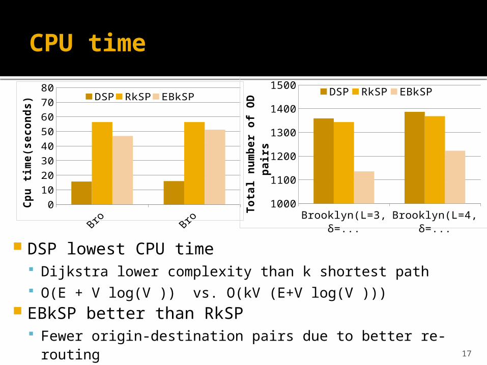
CPU time

DSP lowest CPU time Dijkstra lower complexity than k shortest path O(E + V log(V )) vs. O(kV (E+V log(V )))

EBkSP better than RkSP Fewer origin-destination pairs due to better re-routing

Brooklyn(L=3,δ=0.7)

Brooklyn(L=4,δ=0.7)

0

10

20

30

40

50

60

70

80DSP RkSP EBkSP

Cp

u t

ime(s

econ

ds)

Brooklyn(L=3,δ=0.7)

Brooklyn(L=4,δ=0.7)

1000

1100

1200

1300

1400

1500DSP RkSP EBkSP

Tota

l n

um

ber

of

OD

p

air

s

18

Conclusion & future work

All re-routing strategies decrease significantly the average travel time EBkSP is the best—careful path selection ▪ 104% improvement compared to the “no rerouting” baseline

▪ Lowers with 34% the number of re-routings

Good improvements are observed even for relatively low penetration/compliance rates

To improve scalability and real-time response, we plan to work on hybrid system architectures Offload part of computation to mobile nodes Use ad hoc communication in addition to Internet

communication

19

Thank you !Acknowledgment: NSF Grant CNS-0831753

http://www.njit.edu/~borcea/invent/