Juha Tuomi - TUNIJuha Tuomi Audio-Based Context Tracking Master of Science Thesis ... must provide...

Juha Tuomi

Audio-Based Context Tracking

Master of Science Thesis

The subject was approved by the De-partment of Information Technologyon the of 4th June 2003.Thesis supervisors: Prof Jaakko Astola

DrTech Anssi KlapuriMSc Antti Eronen

Preface

This work was carried out at the Institute of Signal Processing, Department ofInformation Technology, Tampere University of Technology, Finland.

I wish to express my gratitude to my thesis advisor and examiner DrTech AnssiKlapuri for his encouragement, guidance, and patience which enabled me to finishthis long journey and my examiner Prof Jaakko Astola for his advice and comments.

I would also like to thank my advisor MSc Antti Eronen for his invaluable insights,remarks, and suggestions without which this thesis would probably have turned outvery different and MSc Vesa Peltonen for providing me with the initial boost.

I also wish to thank the staff at the Audio Research Group for the wonderful time Ihave had here for the past four years. I have had the privilege of working with someof the smartest and nicest individuals I have ever met.

Finally, I thank Suvi and my parents Terhi and Mikko for all the love and supportthey have given me.

Tampere, December 2004

Juha TuomiTekniikankatu 14 D 17533720 Tamperetel: +358 50 356 2136e-mail: [email protected]

Contents

Tiivistelma iii

Abstract iv

1 Introduction 1

2 Literature Review 3

2.1 Context Awareness . . . . . . . . . . . . . . . . . . . . . . . . . . . . 3

2.2 Implementation on a Portable Device . . . . . . . . . . . . . . . . . . 7

2.3 Audio-Based Context Awareness . . . . . . . . . . . . . . . . . . . . . 10

2.4 General Audio Classification . . . . . . . . . . . . . . . . . . . . . . . 14

3 Acoustic Measurements and Audio Database 18

3.1 Training Set . . . . . . . . . . . . . . . . . . . . . . . . . . . . . . . . 18

3.2 Test Set . . . . . . . . . . . . . . . . . . . . . . . . . . . . . . . . . . 20

4 Feature Extraction Front-End 22

4.1 Preprocessing . . . . . . . . . . . . . . . . . . . . . . . . . . . . . . . 22

4.2 Feature Calculation . . . . . . . . . . . . . . . . . . . . . . . . . . . . 22

4.2.1 Short-Time Energy (STE) . . . . . . . . . . . . . . . . . . . . 23

4.2.2 Zero-Crossing Rate (ZCR) . . . . . . . . . . . . . . . . . . . . 24

4.2.3 Mel-Frequency Cepstral Coefficients (MFCC) . . . . . . . . . 24

4.3 Feature Transforms . . . . . . . . . . . . . . . . . . . . . . . . . . . . 27

4.3.1 Linear Discriminant Analysis (LDA) . . . . . . . . . . . . . . 27

5 Acoustic Modelling and Transition Detection 29

5.1 Gaussian Mixture Models (GMM) . . . . . . . . . . . . . . . . . . . . 29

5.1.1 Description . . . . . . . . . . . . . . . . . . . . . . . . . . . . 29

5.1.2 Training a GMM . . . . . . . . . . . . . . . . . . . . . . . . . 30

CONTENTS ii

5.1.3 Model Order Selection . . . . . . . . . . . . . . . . . . . . . . 32

5.1.4 Using GMMs in Classification . . . . . . . . . . . . . . . . . . 33

5.2 Hidden Markov Models (HMM) . . . . . . . . . . . . . . . . . . . . . 33

5.2.1 Markov Chains . . . . . . . . . . . . . . . . . . . . . . . . . . 34

5.2.2 On Hidden Markov Models . . . . . . . . . . . . . . . . . . . . 35

5.2.3 Using HMMs in Classification (the Evaluation Problem) . . . 36

5.2.4 Forward-Backward Algorithm . . . . . . . . . . . . . . . . . . 37

5.2.5 Finding the Optimal State Sequence (the Decoding Problem) . 38

5.2.6 Viterbi Algorithm . . . . . . . . . . . . . . . . . . . . . . . . . 38

5.2.7 Training a HMM (the Learning Problem) . . . . . . . . . . . . 39

5.3 Algorithms for Context Transition Detection . . . . . . . . . . . . . . 42

5.3.1 Likelihood Criterion for Context Transition Detection . . . . . 42

5.3.2 Indicator Function for Context Transition Detection . . . . . . 44

5.4 On Context Transition Probabilities . . . . . . . . . . . . . . . . . . . 46

6 Real-Time Context Tracking System 48

6.1 Equipment . . . . . . . . . . . . . . . . . . . . . . . . . . . . . . . . . 48

6.2 Baseline Classifier . . . . . . . . . . . . . . . . . . . . . . . . . . . . . 49

6.3 Requirements for Real-Time Context Tracking . . . . . . . . . . . . . 49

6.4 Structure of the Software Suite . . . . . . . . . . . . . . . . . . . . . 51

7 Simulation Results 56

7.1 Context Transition Detection . . . . . . . . . . . . . . . . . . . . . . 56

7.2 Effect of Context Tracking . . . . . . . . . . . . . . . . . . . . . . . . 62

7.3 Computational Load . . . . . . . . . . . . . . . . . . . . . . . . . . . 69

7.4 Analysing the Results and Potential Sources of Error . . . . . . . . . 70

8 Conclusions 72

Bibliography 74

Appendices 77

A Context Transition Matrix 77

B Confusion Matrix for REC 78

Tiivistelma

TAMPEREEN TEKNILLINEN YLIOPISTO

Tietotekniikan osasto

Signaalinkasittelyn laitos

TUOMI, JUHA: Aaneen perustuva kontekstin seuraaminen

Diplomityo, 76 s., 2 liites.

Tarkastajat: prof. Jaakko Astola, TkT Anssi Klapuri

Joulukuu 2004

Avainsanat: aaneen perustuva kontekstin seuraaminen, laskennallinen kuulomaise-man tunnistus, indikaattorifunktio, Gaussin sekoitemalli, katketty Markovin malli

Tama diplomityo kasittelee aaneen perustuvaa kontekstin seuraamista. Tarkoituk-sena on luotettavasti tunnistaa henkilon sosiaalinen ymparisto (konteksti) ja senmuutokset kayttaen ainoastaan yhta mikrofonia. Tietoa kontekstisiirtymista voidaankayttaa vahentamaan tunnistusviivetta ja laskennasta aiheutuvaa kuormaa. Tassatyossa esiteltava jarjestelma, REC, koostuu piirteenirrotusosiosta, kontekstisiirtymanhavaitsemisosiosta ja luokitteluosiosta. Tarkeimmat tyossa kaytetyt piirteet ovatmel-taajuus kepstrikertoimet, nollanylitystaajuus ja signaalin energia. Lineaariselladiskriminanttianalyysilla voidaan pienentaa piirrevektoreiden dimensiota ja kontek-stisiirtymamalli mahdollistaa kontekstien maaran vahentamisen luokitteluvaiheessa.

Diplomityon kirjallisuuskatsauksessa kasitellaan aikaisempia tutkimustuloksia lasken-nalliseen kuulomaiseman tunnistuksen alalla ja siihen laheisesti liittyvilla aloilla.Jarjestelman suorituskykya arvioitiin keraamalla akustinen tietokanta, joka ope-tusvaiheessa koostui 255 keskipituudeltaan noin 3 minuutin mittaisesta naytteestajaettuna 20 kontekstiluokkaan ja 6 korkeamman tason kontekstiluokkaan (metaluok-kaan) seka luokitteluvaiheessa 16 keskipituudeltaan noin 30 minuutin mittaisestanaytteesta, jotka sisaltavat kontekstisiirtymia.

Diplomityon ydin on kontekstisiirtymien havaitsemiseen kehitetty indikaattorifunk-tio, joka simulaatioissa havaitsi kontekstisiirtyman 35% tapauksista (49 havaittuasiirtymaa 139:sta) vaarin luokiteltujen siirtymien osuuden ollessa 3.9% koko testi-joukon pituudesta. Luokittelu kaynnistetaan RECissa indikaattorifunktion havait-tua kontekstisiirtyman. Suorityskykya verrattiin optimoimattomaan luokittimeen jakayttaen samaa HMM:aa 30 sekunnin tunnistuspituudella REC saavutti 50% tun-nistustuloksen (63% metaluokille) kun optimoimattoman luokittimen tunnistustulosoli 49% (66%). REC myos kaytti luokitteluun aikaa noin 50% vahemman.

Abstract

TAMPERE UNIVERSITY OF TECHNOLOGY

Department of Information Technology

Institute of Signal Processing

TUOMI, JUHA: Audio-based context tracking

Master of Science Thesis, 76 pages, 2 enclosure pages

Examiners: Prof Jaakko Astola, DrTech Anssi Klapuri

December 2004

Keywords: audio-based context tracking, audio-based context awareness, indicatorfunction, Gaussian mixture model, hidden Markov model

This thesis addresses the problem of audio-based context tracking, i.e. recognis-ing the social situation (context) around a person using audio only and reacting tochanges in the context. We propose a system, REC, for detecting context transi-tions while minimising the recognition latency and computational overhead. RECconsists of a feature extraction front-end, a context transition detection part, and aclassification part. The main features used are mel-frequency cepstral coefficients,zero-crossing rate, and short-time energy. The system supports the use of linear dis-criminant analysis for reducing the feature dimensionality and a context transitionmodel for reducing the amount of possible contexts during the classification.

We present a literature review discussing previous work on audio-based contextawareness and related fields of interest. An acoustic database consisting of 255recordings with an average length of about 3 minutes was gathered and divided into20 contexts and 6 higher-level contexts (metaclasses) for training and 16 recordingswith an average length of about 30 minutes containing context transitions were usedfor classification.

The focus of this thesis is in detecting context transitions and the proposed indi-cator function could detect these transitions with an accuracy of 35% (49 detectedtransitions out of 139) while the amount of incorrectly detected transitions was 3.9%of the test set length. The classification in REC is initialised when the indicatorfunction detects a context transition. A comparison between an unoptimised classi-fier and REC is presented and the results using the same HMM for a classificationlength of 30 seconds were 50% (63% for metaclasses) for REC versus 49% (66%) forthe unoptimised classifier. REC also reduced the total classification time requiredby about 50% compared to the unoptimised classifier.

Chapter 1

Introduction

During the last 50 years, we have seen a shift from huge, mainframe-based computersto pocket-sized mobile devices while the available processing power has increasedexponentially. Since mobile devices such as cellular phones and personal digitalassistants (PDAs) are cheaply available people carry and use these devices practicallyeverywhere they go. The social impact of these mobile devices is not yet fullyknown and in the future it may prove advantageous for the devices to be able todiscern between various social environments (contexts) and alter their behaviouraccordingly. For example, a cellular phone could observe its current environmentand adjust the ring tone to be louder when on a crowded street or quieter when ina church or a library. This is called context awareness.

To study context awareness we must first define what the term means. In [Cla02],Clarkson describes a context-aware agent1 as an agent which has sensors into theuser’s physical world and the ability to learn the basic rules of that world. Thus acontext-aware agent can react to events in its surroundings without explicit directionfrom the user.

In [Tuu00], Tuulari defines context awareness as “knowledge of the environment,location, situation, user, time, and current task”. It can be exploited in selecting anapplication or information, adjusting communication and adapting the user interfaceaccording to the current context. A self-contained context-aware agent can achievecontext awareness without any outside support. In contrast, an infrastructure-basedcontext-aware agent requires support from a larger external system or infrastructureto recognise its context.

For the scope of this thesis, we define the term context awareness as a process inwhich a device utilises sensors to extract information about its user’s social context2

and reacts to this extracted information. The sensors used can measure any attributeof the surrounding environment and the user, such as the temperature, lighting, noiselevel, speed or acceleration of the sensor in relation to the environment, and datafrom different types of sensors can be combined. In this thesis, only audio sensors(microphones) are used to extract contextual information.

1An agent can be a software or a hardware component.2Different social contexts include for example sitting in a restaurant, giving a lecture, or driving

a car.

2

We also define the term context tracking as a context-aware process, in which weutilise causality and information about context transitions to improve the speed andreliability of the classification. The first challenge of this task is in increasing thespeed (reducing the algorithmic delay) of the classification process at context transi-tions, possibly utilising information about prior contexts and transitions. The secondchallenge is in maximising the recognition accuracy of the system while maintaininga low computational load. We believe a reasonable compromise can be achievedbetween recognition accuracy and computational load by stripping the classificationprocess into a bare minimum: the system described in this thesis only classifies anauditory scene when it detects a change in the auditory characteristics of its currentenvironment.

Since context tracking is a generalisation of context awareness there has been plentyof research related to the awareness part of the problem. Most of the studies havebeen conducted using off-line classification with ample computing resources. Sincetime is usually not a limiting factor, the systems can be as elaborate and largeas desired and most of the systems are based on continuous classification of theincoming audio samples. However, implementing them in mobile environments,where processor time is precious and memory is limited, is not always very practical.The classification can be lightened by using simpler features, lower sampling rates,and light-weight classifiers, but the basic idea of continuous classification still holds.

The research reported in this thesis extends the research of MSc Vesa Peltonenand MSc Antti Eronen, who have presented useful features, methods, and trainingand classifying schemes to recognise everyday auditory contexts. We extend thisresearch from off-line recognition of discrete sound samples to being closer to the”real world” situation where the classification is performed in a continuous mannerusing the audio data from the user’s environment. The main purpose of this thesisis to study how well the computer can handle transitions, both rapid and slow, fromone auditory context to another and how information about transitions can be usedto speed up the classification process.

In Chapter 2, we present a literature review on the current state of the research incontext awareness and related fields of interest. In Chapter 3, the audio databasecollected for this thesis is presented and the recordings containing context transitionsare discussed. Chapter 4 describes the feature extraction front-end, the auditoryfeatures used in this thesis, and the applied parameter values. Chapter 5 is themain part of this thesis. It discusses the mathematical models and algorithms usedin depicting the data, the training procedure, context transition detection and otherspeed-up methods, and the algorithmic complexity and memory consumption ofthe selected algorithms. Chapter 6 presents an overview of the context trackingsystem, the equipment required, the structure of the classification system, and itsrequirements. Chapter 7 describes the results obtained in the conducted simulations.Finally, Chapter 8 summaries the thesis and discusses possible directions for futurework.

Chapter 2

Literature Review

This chapter discusses context awareness in general, implementations of contextawareness in mobile devices, audio-based context awareness, and general audio clas-sification. Research papers on the topics are discussed and results are given whenapplicable. A survey of context-aware mobile computing has been earlier describedin [CK00].

2.1 Context Awareness

General Model of Context Awareness

In [RJP04], Roman et al. presented an abstract conceptual model and formalisationof context awareness. An application can be called context-aware (qualifies as aninstance of the context-aware paradigm) if it meets the proposed model requirements:expansiveness, specificity, explicit notion of context, separability, and transparency.The system presented in this thesis conforms with these model requirements in thesense that it is expansive (no a priori assumptions about the scope of the contextswere made), specific (the list of available contexts can be tailored for each instanceof the system), has an explicit notion of context (the context is the most probablecontext given a set of parameters, an inner model), separable (the functionality of thesystem is separated from the definition of context) and transparent (the definitionof context is made available to the underlying infrastructure at run time). Thereforethe system presented in this thesis can be called context-aware.

The model proposed by Roman et al., Context UNITY, assumes that the system ispopulated by a given set of agents who have a finite set of behaviour types (function-alities). At the abstract level, each agent is a state transition system, and contextchanges are perceived as spontaneous state transitions outside of the agent’s con-trol. The model’s context rules enable the separation, decoupling, of the applicationcode from the definition of context, which is important in systems requiring adapt-ability since the program cannot anticipate the possible details of the operationalenvironments it will encounter.

2.1 Context Awareness 4

Designing Context-Aware Applications

There are a number of taxonomies for the features1 of context-aware applications[SAW94, Pas98]. In his doctoral thesis [Dey00], Dey divided the context-awarefeatures which devices may support into three categories:

1. presentation of information and services to the user, such as a laptop computerwhich dynamically updates the list of closest printers while on the move,

2. automatic execution of a service, for example when printing a document it isprinted on the closest printer to the user, and

3. tagging of context to information for later retrieval, such as logging the namesof the printed documents, the times when they were printed and the printerused.

This categorisation has two benefits: first, it specifies the types of applications onemust provide support for, and second, it shows the types of features one shouldbe thinking about when building context-aware applications. Dey also proposeda design process for building context-aware applications which is divided into fivesteps:

Specification Specify the problem being addressed and a high-level solution

Acquisition Determine what new hardware or sensors are needed to provide con-texts

Delivery Provide methods to deliver the context to (remote) applications

Reception Acquire and work with the context

Action If context is useful, perform context-aware behaviour

The process can further be simplified to contain only some of the tasks in the essen-tial specification, acquisition and action steps.The conversion of the received contextinformation into a useful form (classification) is conducted in the acquisition stepeither by the sensors or the application. Both the conversion and storage of contextinformation are considered accidental (only necessary when there is no existing sup-port for these tasks available). The analysis of the context is performed in the actionstep but it is also considered accidental and should be provided by the underlyingsupport infrastructure.

Quality of service metrics such as accuracy, reliability, coverage, resolution, fre-quency, and timeliness are also discussed. Of these, frequency and timeliness are themost important when considering the “real-time” characteristics of a context-awaresystem. Frequency defines how often the context information is updated. Timelinessdefines the allowed time between the actual context change and its notification. In

1These are not to be confused with the transforms of the measurements taken by the sensors inthe context-aware system, which are also called features.


context-aware applications, both are usually limited by the capabilities of the sys-tem, high frequency and low latency (timeliness) lead to a high computational loadwhich is unwanted in real-time applications such as the Real-Time Context TrackingSystem described in this thesis.

Dey et al. noted that most current context-aware services make the assumption thattheir context data is always accurate [DMAC02]. This, however, is seldom the caseand there have been many attempts to improve accuracy in sensing the contextincluding the design of more accurate sensors and the use of sensor fusion [BI97]. Ifthe system would alert the user that the context is inaccurate, the user could takesteps to mediate or correct the context data before any irreversible action occurs.This mediation can be in the form of prompting the user for more information whenthe current context is ambiguous or presenting the user with various options andtheir relevances to the current task.

Opposed to the more general definition of context awareness in [RJP04], Dey de-scribed the required supporting framework and design process for building context-aware applications. The design process can be used by others to speed up thedevelopment of context-aware applications since the required design tasks are al-ready known. Dey’s definition of context awareness can also be used to evaluatewhether or not a particular application can be called context-aware: it does not re-quire the application to adapt to the current context, but merely to provide relevantinformation and/or services to the user depending on his current task. Roman etal. described the formal requirements for creating a model for an arbitrary context-aware application while Dey discussed the design and implementation of the actualapplication.

Study on Human Interruptibility

Since computer systems are generally unaware of the characteristics of the contextin which they operate they typically have no way to take the interruptibility ofthe user into account. In [HFA+03], Hudson et al. conduct a study on how robustpredictions of interruptibility can be made, what kind of sensors might be mostuseful to these predictions, and how simple such sensors might be. For the study,they collected 602 hours of video with audio from four different test subjects attheir place of work. Each test subject was frequently interrupted at their office by“walk-in” requests from a number of different people. The subjects were given anaudio prompt at random but controlled intervals, up to two times per hour, in whichthey were asked to describe their current interruptibility using a scale from one tofive, with one being the most interruptible. This rating could be given verbally orby holding up some fingers on one hand to the camera. The data was processed andcoded manually in 15 second sequences by multiple coders utilising the interface in[HFA+03, Figure 1].

The data was collected from a total of 672 prompts. In 8.0% of the cases the subjectdid not report to the prompt and these situations were classified as being in the“leastinterruptible” category, also removing these cases had very little effect on the finalpredictions. The simulated sensors, features, were binary and were chosen becausethey were a priori believed to be correlated with interruptibility. There were 23


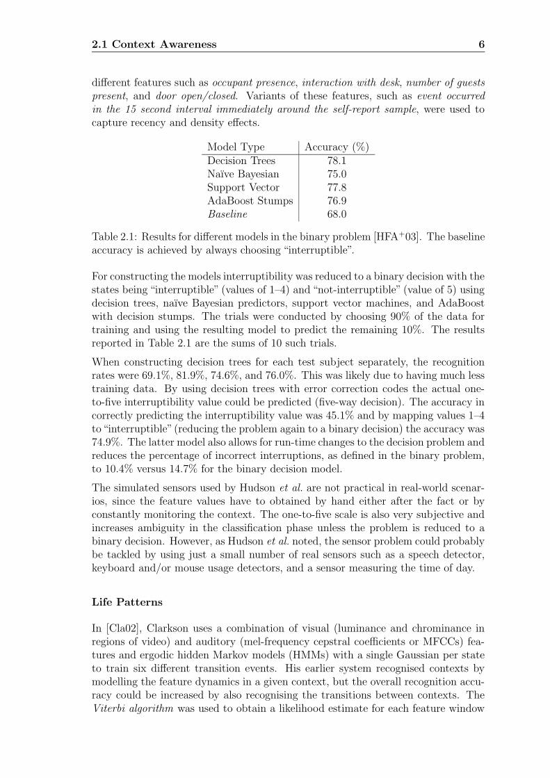
different features such as occupant presence, interaction with desk, number of guestspresent, and door open/closed. Variants of these features, such as event occurredin the 15 second interval immediately around the self-report sample, were used tocapture recency and density effects.

Model Type Accuracy (%)Decision Trees 78.1Naıve Bayesian 75.0Support Vector 77.8AdaBoost Stumps 76.9Baseline 68.0

Table 2.1: Results for different models in the binary problem [HFA+03]. The baselineaccuracy is achieved by always choosing “interruptible”.

For constructing the models interruptibility was reduced to a binary decision with thestates being “interruptible” (values of 1–4) and “not-interruptible” (value of 5) usingdecision trees, naıve Bayesian predictors, support vector machines, and AdaBoostwith decision stumps. The trials were conducted by choosing 90% of the data fortraining and using the resulting model to predict the remaining 10%. The resultsreported in Table 2.1 are the sums of 10 such trials.

When constructing decision trees for each test subject separately, the recognitionrates were 69.1%, 81.9%, 74.6%, and 76.0%. This was likely due to having much lesstraining data. By using decision trees with error correction codes the actual one-to-five interruptibility value could be predicted (five-way decision). The accuracy incorrectly predicting the interruptibility value was 45.1% and by mapping values 1–4to“interruptible”(reducing the problem again to a binary decision) the accuracy was74.9%. The latter model also allows for run-time changes to the decision problem andreduces the percentage of incorrect interruptions, as defined in the binary problem,to 10.4% versus 14.7% for the binary decision model.

The simulated sensors used by Hudson et al. are not practical in real-world scenar-ios, since the feature values have to obtained by hand either after the fact or byconstantly monitoring the context. The one-to-five scale is also very subjective andincreases ambiguity in the classification phase unless the problem is reduced to abinary decision. However, as Hudson et al. noted, the sensor problem could probablybe tackled by using just a small number of real sensors such as a speech detector,keyboard and/or mouse usage detectors, and a sensor measuring the time of day.

Life Patterns

In [Cla02], Clarkson uses a combination of visual (luminance and chrominance inregions of video) and auditory (mel-frequency cepstral coefficients or MFCCs) fea-tures and ergodic hidden Markov models (HMMs) with a single Gaussian per stateto train six different transition events. His earlier system recognised contexts bymodelling the feature dynamics in a given context, but the overall recognition accu-racy could be increased by also recognising the transitions between contexts. TheViterbi algorithm was used to obtain a likelihood estimate for each feature window

2.2 Implementation on a Portable Device 7

and the event exceeding a given threshold was triggered. The thresholds were ob-tained by calculating the receiver-operator characteristic (ROC) for each model andusing the equal error rate (EER) criterion to determine the optimal points on theROC curves2.

Clarkson examined transitions in three different locations: an office, a kitchen anda “black couch area” (BCA). For each model, the optimal number of states and thewindow size was found using a brute-force approach over a selected range and theresults can be found in Table 2.2.

Event Number of Number of Window size Accuracyexamples states (s) (%)

Leave Office 31 8 20 85.8Enter Office 27 2 11 92.5Leave BCA 21 3 20 92.6Enter BCA 22 7 20 95.7Leave Kitchen 21 1 4 99.7Enter Kitchen 22 7 11 94.0

Table 2.2: Model parameters and accuracies for each transition event [Cla02]

Clarkson’s use of temporal constraints for limiting complexity and boosting perfor-mance is very similar to the higher-level context transition model proposed in thisthesis. A table of conditional probabilities, such as the one described in [Cla02, p.45], was realized in this thesis and is described in Appendix A. As in this thesis,Clarkson selected an ergodic HMM for modelling the temporal signatures of a situa-tion since no a priori assumptions can be made about the situation dynamics. Theused time scale of 2 seconds would seem to be adequate for capturing the intricaciesof a given context.

2.2 Implementation on a Portable Device

TEA Project

The TEA project (Technology for Enabling Awareness, [VL99], [VL00]) was a jointproject funded by the European Commission Esprit Program. Its objective wasto study context awareness in wearable and hand-held devices using low-cost andwidely available sensors. Van Laerhoven’s system [VL99] consisted of four layers: thefirst layer represents the acquisition of raw data from low-level sensors, the secondlayer extracts cues from the output of the first layer, the third layer maps these cues

2A ROC curve shows the probability of a false positive classification on the x-axis and theprobability of a true positive classification on the y-axis. ROC curves are used in recovering theclass probabilities from the HMM log-likelihoods by determining

Ithreshold = φ−1(pthreshold) = φ−1(0.5), (2.1)

where φ is a continuous mapping function which assigns all log-likelihoods to [0,1] withφ(Ithreshold) = 0.5. This is valid for 2-class problems.


into a context profile given by the user and the fourth layer uses this information tochange the behaviour of the application according to current context.

Since a sensor such as a microphone can output large amounts of data in a shortperiod of time, it is not reasonable to use this raw data as the input to the contextrecognition system. In practical applications the input of the recognition systemdoes not have to be updated every time the sensors output new data. By usingfeatures such as the mean and/or variance of the sensor outputs over a certainperiod of time (when using a light sensor, for example) the amount of processingcan be significantly reduced and the robustness of the system increased, since novalues have to be discarded. These features and others such as filtered outputs andtransformations of the sensor data are called cues.

[VL99] focused primarily on the third layer. It is a learning system and is requiredto be adaptive, transparent to the user, and as autonomous as possible. Trainingwas realized by clustering the cues using Kohonen self-organising maps (KSOM) andby associating each cluster with a user-defined context. When using a large numberof sensors, the size and complexity of the SOM increases dramatically reducing itsusefulness in on-line applications. Laerhoven handled this problem of dimensionalityby dividing the input space into subsets using an intermediate layer. This had theeffect of excluding potentially relevant sensor combinations. The results then hadto be combined to form the output of the intermediate layer. HMMs were used inthe classification phase since they model probable sequences of contexts and allowfor a crude model of user behaviour.

Laerhoven reported improvement on the recognition rate when reducing the inputspace dimensionality but due to the simplicity of the experiment (only a minimalamount of training for each context, practically random selection of the used sensorsubsets, and no information given about overlapping in the sensor subsets) it cannotbe conclusively said that this “divide-and-conquer” approach was the reason for theimproved recognition rates. This reduction in the input space dimensionality couldalso be achieved using some type of data-driven linear transform as discussed inSection 4.3.

Nomadic Radio

In his Master’s thesis [Saw98], Sawhney described a wearable audio platform knownas Nomadic Radio, which provided the user with an audio-only interface to unifyremote information services such as e-mail, voice mail, news broadcasts and calendarfunctions. Nomadic Radio used ambient auditory cues to inform the user of newmessages and events in the background while constantly monitoring the user’s envi-ronment. To recognise conversation and avoid unnecessary distraction to the user, acollection of fully connected HMMs using 1-15 states, depending on the complexityand duration of the sound being modelled, were trained to detect the presence of for-mants in voiced speech. The system had separate models for a number of male andfemale speakers to reliably detect any speech regardless of the speaker and Sawhneyclaimed the implementation ran in real-time on a Pentium-class PC.

Sawhney’s implementation was designed to be as unobtrusive and easily usable aspossible, since the idea was for the users to carry the application around wherever


they go. The Nomadic Radio application was also multi-modal, i.e. it could accepteither speech or tactile input. The use of ambient auditory cues to inform the userof the priority of the incoming message (based on the message type) is a fairly goodsolution to the interruptibility problem, since a distinct auditory cue such as a loudbeep is usually much more distracting than only a slight change in the ambientauditory background.

Sound Classification for Hearing Aids

In [NL04], Nordqvist and Leijon presented a sound classification algorithm based onHMMs for hearing aids. The purpose of the algorithm was to enable a hearing aid toadapt to its current listening environment depending on its user’s preferences. Cur-rent hearing aids have limited computing resources and thus their sound classificationsystems have traditionally had low complexity and were typically threshold-based orBayesian classifiers tasked mainly with controlling noise reduction and directionality.The behaviour of the hearing aid is most commonly controlled by the user switch-ing between different programs using a button on the hearing aid. This presentsproblems to passive users and people who are unable to operate the button on thehearing aid.

Nordqvist and Leijon trained a four-state ergodic sound-source HMM using fourvector-quantised delta-cepstrum coefficients as features. The purpose of the sim-ulation was to distinguish between three distinct listening environment categories:“speech in traffic noise”, “speech in babble”, and “clean speech”, regardless of thesignal-to-noise ratio (SNR). Each sound source – “traffic noise”, “babble”, and “cleanspeech” – was modelled with one HMM and the resulting listening environment wasdefined as a single sound source or a combination of two sound sources and pro-cessed by a five-state environment HMM in hierarchical fashion. The environmentHMM consisted of a “speech in traffic noise” environment (state E(t) = 1) contain-ing the traffic noise model (state S(t) = 1) and speech model (state S(t) = 2), the“speech in babble” environment(state E(t) = 2) containing the babble model (stateS(t) = 3) and speech model (state S(t) = 4), and the “clean speech” environment(state E(t) = 3) containing only the speech model (state S(t) = 5). Transitionsbetween listening environments had low probabilities and transitions between statesin one listening environment had relatively high probabilities.

Nordqvist and Leijon used non-overlapping sets of training and evaluation materialto assess the performance of the system. The training material consisted of 26recordings containing “clean speech”, “babble noise”, and “traffic noise” totalling838 seconds. The evaluation material consisted of 99 recordings containing “cleanspeech”, “babble noise”, “traffic noise”, and “other noise” totalling 3299 seconds.Table 2.3 presents the obtained classification results for the simulation.

A false alarm occurred for the given environment category if a test segment wasincorrectly classified as belonging to that category. Nordqvist and Leijon reportedclassifier output latencies, measured as the time it took for the classifier outputto shift from one environment category to another after the stimulus changed, ofaround 2–3 seconds for the “clean speech” environment and 5–10 seconds for theothers. The estimated computational load was around 0.1 million instructions per

2.3 Audio-Based Context Awareness 10

Environment Hit rate (%) False alarm rate (%)Speech in traffic noise 99.5 0.2Speech in babble noise 96.7 1.7Clean speech 99.7 0.3

Table 2.3: Classification results reported in [NL04]

seconds (MIPS) and the estimated memory consumption was around 700 words ona Motorola 56k or equivalent architecture, assuming a computational overhead of50%.

The use of hierarchical HMMs is a good way to increase the generalisation capabil-ities of the model and to reduce the computational complexity. It is however notsuited for all applications since it can sometimes be difficult to break an elaboratemodel into smaller, “atomic” models. In the case of auditory context awareness,one possible implementation of a hierarchical HMM could be for example to grouprelated sound sources (contexts) such as “car”, “bus”, and “train” into a higher-levelcontext, “vehicle”. Thus even if the actual context is incorrectly detected, the higher-level context could be correctly detected. If the contexts were grouped wisely, thebehaviour of the application should not be much different for contexts within agroup.

2.3 Audio-Based Context Awareness

Audio-based context awareness refers to the process of recognising environments us-ing audio information only [PTK+02]. It is a subproblem of computational auditoryscene analysis (CASA), which refers to the computational analysis of an acoustic en-vironment and the recognition of distinct sound events in it. The process of auditoryscene analysis in humans has been described in [Bre90].

Off-line Classification of Everyday Auditory Scenes

In [Pel01], Peltonen analysed the efficiency of various features and classifying algo-rithms in recognising everyday auditory contexts. The audio database consisted of124 samples in 25 different contexts, of which 13 contexts were used in the classifi-cation. It is a subset of the database used in this thesis (Table 3.1) and is describedin [Pel01, p. 15].

Peltonen evaluated the performance of a Gaussian mixture model (GMM) classifierwith varying amounts of Gaussian components and a test sequence length of 30seconds. Using 12 MFCCs Peltonen obtained a recognition rate of 56.79% with fourGaussians.

Peltonen observed that the performance of the recognition system depends more onthe feature set than the classifier. A recognition system comprising a one-nearest


neighbour (1-NN) classifier with band-energy ratio (BER3) averaged over one secondwindows yielded a 56% recognition rate for a test sequence length of 15 seconds, whilethe GMM classifier with MFCCs gave a 57% recognition rate for a test sequencelength of 30 seconds.

In [PTK+02], the first order time derivatives or deltas of the auditory features wereincluded but the overall recognition rate deteriorated. Using leave-one-out crossvalidation, a training sequence length of 160 seconds and a test sequence length of30 seconds, the performances of different classifier/feature combinations are shownin Figure 2.14.

1 2 3 4 50

10

20

30

40

50

60

70

80

Rec

ogni

tion

accu

racy

(%)

Feature set and classifier

Figure 2.1: Results for different classifiers and feature sets [Pel01]. Their descriptionscan be found in Table 2.4.

Set Classifier Features1 1-NN (mean+std) Band energy (10), spectral flux,

spectral roll-off point, spectral centroid (SC),zero-crossing rate (ZCR)

2 GMM (5) MFCC (12)3 1-NN (mean+std) Band energy (10)4 1-NN (mean+std) Band energy (10), delta band energy (10)5 1-NN (mean+std) Delta band energy (10)

Table 2.4: Classifiers and feature sets in Figure 2.1

The drop in recognition accuracy when using the delta features was due to thefact that the delta features were not mean and variance normalised, so their dy-

3BER is defined as the ratio of the energy in a given frequency band to the total energy overall frequency bands. BER for the ith sub-band is calculated as

BERi =∑

n∈Si

|X(n)|2/

M∑

n=0

|X(n)|2 (2.2)

4(mean+std) The mean and the standard deviation (std) of the features over one second windowswere used with the intention of modelling the slow-changing attributes of the auditory scene.


namic range became too small causing computational problems when performingcalculations in a linear space. Even though the best result was obtained using acombination of five features, it was not necessarily optimal since all the possible fea-ture combinations could not be studied due to the enormous amount of computingrequired.

Acoustic Modelling and Perceptual Evaluation

In [ETK+03], a listening test to study the human ability to recognise contexts basedonly on auditory signals was conducted in order to obtain a baseline for the assess-ment of computational model performance. For the sake of comparison, a computersystem was then trained using appended vectors of 11 MFCCs and their 11 first timederivatives as features and two-state fully connected HMMs with two Gaussians com-ponents per state. The feature vectors were both mean and variance normalised andthe 0th coefficients were discarded.

The test setup consisted of two non-overlapping sets of 45 samples from 18 differentcontexts in the test set and all the remaining 180 samples were used in the trainingset. The length of the samples in the training set was 160 seconds and the lengthof the classified samples was 60 seconds. The contexts were a subset of the audiodatabase described in Table 3.1. Each context was also assigned to one of the higher-level classes which were “outdoors”, “vehicles”, “public places”, “offices/quiet places”,“home” and “reverberant places”. Figure 2.2 shows the results of the comparisonbetween the human and the computer performance.

0 10 20 30 40 50 60 70 80 90 100

Context

Higher−level class

Recognition accuracy(%)

ComputerHuman

Figure 2.2: Results of the listening test [ETK+03]

Even though the training and test sets were not entirely the same between [PTK+02]and [ETK+03], some comparisons can be made. First, the mean and variance nor-malisation of the features had a positive effect on the recognition rate. Second,


Eronen achieved a notable increase in the the recognition rate by using only a low-complexity HMM (2 states with one Gaussian component per state compared toa GMM with 5 Gaussian components in [PTK+02]). This is in some part due tothe fact that the situation dynamics of an auditory context can be modelled betterwith a HMM than with a GMM. Third, even though Eronen used a test sequencelength of 60 seconds (twice the amount of data per test sample than Peltonen5), itwas observed in [PTK+02] that an increase in the test sequence length has only anegligible effect on the recognition rate when comparing a test sequence length of30 seconds to 60 seconds. Peltonen also used leave-one-out cross validation whichyielded a larger amount of training data for each context.

Context-Aware Notification for Wearable Computing

In [KS03] the problem of classifying the social situation of the user was discussed.Kern and Schiele proposed a system consisting of two-state ergodic HMMs with sixdifferent acoustic features based on the spectral centroid, the tonality of the signal,the amplitude onsets, and the amplitude histogram width. The input spectrumwas divided into 20 Bark bands and an amplitude onset was defined by observingthe changes between successive frames within the bands. The amplitude histogramwidth was defined as the width between the 10th and 90th percentiles of the amplitudehistogram, obtained by taking the maximum from 3 ms sub-frames (scaled to dBunits).

To examine the performance of the system, a database consisting of 54 one-minutesamples was used. The samples were divided into four classes: Street (17 samples),Restaurant (15), Lecture (12) and Conversation (10). Kern and Schiele reportedan overall recognition rate of 83.17% using 5-fold cross validation. The confusionmatrix for the test is described in Table 2.5.

Discrimination resultContext Street Restaurant Lecture ConversationStreet 82.35 17.65

Restaurant 6.67 86.67 6.67Lecture 91.67 8.33

Conversation 28.00 72.00

Table 2.5: Confusion matrix for the system proposed by Kern and Schiele [KS03]

Kern and Schiele also tested their context-aware system by recording 38 minutes ofcontinuous audio and acceleration data from a variety of different situations. Theset also contained locational data from Wireless LAN access points. The recordingincluded contexts such as a laboratory, walking on a street, discussions, a lectureand a restaurant divided into five classes: “conversation”, “lecture”, “restaurant”,“street” and “other”.

The audio classification was done every ten seconds since the auditory scenes werechanging slowly. The context recognition based on the acceleration signal was done

5Peltonen also used 26 possible contexts while Eronen used only 24.

2.4 General Audio Classification 14

at a frequency of 55 Hz and the possible classes were “sitting”, “standing”, “walking”and “stairs”. Classification was done using the Bayes’ rule.6 Kern and Schielealso gathered data from Wireless Access Points for locational context to be usedas the ground truth in the experiment. The access points were grouped into fivegroups: “office”, “outdoor” (no access point), “lecture hall”, “lab” and “cafeteria”.The reported recognition rate using the acceleration sensor was 91.9% but for theauditory context the rate was only 65.5%.

Kern and Schiele distinguished between the user’s personal interruptibility (depend-ing on the current activity of the user) and social interruptibility (depending onthe current social situation of the user) in order to adapt the notification schemefor different scenarios. This is beneficial if the application has a number of ways ofnotifying the user such as auditory cues, visual cues, or physical activity (vibrationetc). The system proposed in this thesis, however, has only one mean of notifyingthe user and that is a visual cue (displaying the current context). Therefore theuser’s personal interruptibility can be ignored, since the user will not see the visualcue if he is involved in some other activity. An actual mobile application based onthis system should nonetheless take the user’s personal interruptibility into accountif the notification scheme demands it.

2.4 General Audio Classification

In recent years, researchers of automated speech recognition (ASR) have shifted theirfocus towards classifying general audio data (GAD). To improve the recognitionrates of ASR systems, general audio classification can be used as a preprocessingstep to allow the system to employ the correct acoustic model for each homogeneoussegment of the audio signal, representing a single class [LSDM01].

A general audio signal can consist of almost any type of signal imaginable, for exam-ple speech, music, environmental sounds and noise. Different sources of audio signalscan be characterised by various acoustic and linguistic conditions and the qualityof the data depends highly on the transmission channel. In information retrievalsystems, methods for indexing the content of general audio data are becoming moreimportant and automated indexing methods would allow the users browsing audiodata to skip over uninteresting parts to indices containing important acoustic cues[Spi00].

6The Bayes’ rule is defined as

P (A|B) =P (B|A)P (A)

P (B), (2.3)

where P (A|B) is the posterior probability or the probability of model A given evidence B, P (B|A)is the likelihood of evidence B given model A, P (A) is the prior probability of model A, and P (B)is the probability of evidence B.


A Hierarchical Method of Audio Classification

An algorithm for robust audio classification was presented by Lu et al. in [LJZ01].By using a 2-nearest neighbour classifier and linear spectral pairs7–vector quantisa-tion (LSP-VQ) analysis, the input signal was classified into speech and non-speechsegments. In the second phase, non-speech signals were further classified by a rule-based scheme into music, environmental sound and silence.

The features used in the first phase were high zero-crossing rate ratio (HZCRR),which is defined as the ratio of the number of frames whose ZCR are above 1.5times the average zero-crossing rate in a one-second window, low short-time en-ergy ratio (LSTER), which is defined as the ratio of the number of frames whoseshort-time energy are less than 0.5 times the average short-time energy in a one-second window, and spectrum flux. In classifying non-speech signals, silence wasfirst detected by comparing the short-time energy and ZCR in one-second windowsto a given threshold. If the signal was not classified as silence, it was classifiedinto music or environmental sound by comparing band periodicity (BP), which isdefined as the periodicity of each sub-band (represented by the maximum local peakof the normalised correlation function), spectrum flux and noise frame ratio (NFR)against further thresholds in a hierarchical process. All the thresholds were obtainedexperimentally.

Lu et al. reported that the system was capable of correctly classifying general au-dio into three classes with an overall accuracy of 96.51%. For speech/music dis-crimination, the accuracy was 98.03%. Table 2.6 shows the confusion matrix forspeech/music/environmental sound classification.

Discrimination resultSound type Speech Music Env soundSpeech 97.45 1.55 1.00Music 3.16 93.04 3.80

Env. sound 10.49 5.08 84.43

Table 2.6: Confusion matrix for the system proposed by Lu et al. [LJZ01]

Lu et al. claimed that HZCRR and LSTER are good features for characterisingdifferent types of audio signals such as speech, music, or environmental sounds.Since they are only modifications to zero-crossing rate and short-time energy, theyare still computationally fairly light features and could thus prove useful for mobileapplications such as the one proposed in this thesis. Even though Lu et al. reportedexcellent recognition rates it should be noted that using only four classes (five ifsilence is included) yields a random guess rate of 25%. Also the thresholds have tobe obtained experimentally for each individual application.

7Linear spectral pairs (LSP) is another representation of the coefficients of the inverse filterA(z) obtained from the linear prediction coefficients (LPC).


The MPEG-7 Standard

In [Cas02], Casey described some of the tools available for managing complex soundcontent in the MPEG-7 standard8. By using data-derived basis functions obtainedby methods such as principal component analysis (PCA9) [Jol86], singular value de-composition (SVD) [SWS02] and independent component analysis (ICA) [HKO01],the dimensionality of the feature data can be reduced while retaining the maximumamount of information.

The MPEG-7 standard also allows the use of taxonomies or hierarchical trees con-sisting of a number of sound categories. Their purpose is to provide semantic rela-tionships between categories, for example a sound classified as a “dog bark” inheritsthe label “animal”, since each sound segment categorised in a leaf node inherits thecategory label of its parent node in the taxonomy.

Casey used de-correlated spectral features and trained 19 continuous HMMs usingmaximum a posteriori (MAP) estimation on a database of over 2000 sounds dividedinto 19 different classes. He split the database in two, using 70% of the sounds totrain the HMM models and 30% to test the recognition rate on novel data. Thereported mean recognition rate was 92.646%. The results of the test for individualclasses are shown in Figure 2.3.

50 55 60 65 70 75 80 85 90 95 100

AltoFluteBirds

PianosCellos

ApplauseDog Barks

English HornExplosionsFootsteps

Glass SmashesGuitars

Gun ShotsShoes

LaughterTelephones

TrumpetsViolins

Male SpeechFemale Speech

Recognition accuracy(%)

Figure 2.3: Recognition rates for the 19 classes [Cas02]

The MPEG-7 description definition language (DDL) is a formal and generaliseddescription of data and a variety of statistical methods for feature extraction andgeneral sound classification, which in theory should improve interoperability between

8MPEG-7, formally named “Multimedia Content Description Interface”, is a standard for de-scribing the multimedia content data that will support some degree of interpretation of the infor-mation’s meaning, which can be passed onto, or accessed by, a device or a computer code (from[Mov01]).

9PCA is used to determine a linear transformation for vector x such that on the new principal

axes the samples are de-correlated. Thus it provides an orthogonal basis for a given data set.


different applications. Up to this point, applications have generally used proprietaryand/or incompatible implementations of classifying and indexing sound content eventhough many of them were based on the exact same features and methods. The de-scriptors and description schemes contained in the MPEG-7 toolkit represent a goodcross-section of the current state-of-the-art in sound similarity rating and classifi-cation and since DDL allows extensions to the current descriptions and descriptionschemes, anyone can introduce novel tools into the public domain.

Chapter 3

Acoustic Measurements and AudioDatabase

The acoustic database used in this thesis was collected in three parts between theyears 2000 and 2004. The recordings were made in everyday environments such asstreets, shops, restaurants, cars, and kitchens using three different recording setups.The first recording set was collected to obtain discrete samples from a wide variety ofcommon auditory environments to be used in the training phase. These recordingsrange in length from approximately 160 seconds to over 10 minutes, with most ofthe recordings being 3–5 minutes in length.

The second set of recordings was collected in order to evaluate the performance ofthe context tracking system and it consists mostly of long, continuous recordingswith context transitions. Some of these continuous recordings were also dividedinto discrete contexts to be used in the training phase and were excluded from theevaluation set.

A total of 20 context labels were grouped into six higher-level classes and are listed inTable 3.1. However, it should be noted that it is not always easy to categorise a givensample since it can fall under different context labels. The number of recordings usedin the training is also listed for each context. The samples were all recorded using16-bit precision and 48 kHz sampling rate.

3.1 Training Set

The acoustic data for the training phase was collected in many parts. In each case,we used AKG C460B microphones for the recordings. Recording setup 1 was an8-channel setup consisting of a binaural part (2 channels), stereo part (2 channels),and a B-format part (4 channels). This setup was developed by Zacharov andKoivuniemi [ZK01] and is described in detail in [Pel01, pp. 12-13]. Only the datafrom the stereo channels for each recording were used. A total of 55 recordings usingthis setup were included in the database.

Recording setup 2 was designed to be more portable than setup 1 for the purposeof obtaining a larger amount of samples from different contexts. It consisted of a

3.1 Training Set 19

two-channel stereo setup and a DAT recorder and the configuration is described in[Pel01, pp. 13-14]. The highpass filter in the stereo preamplifier was set to 80 Hzfor all the recordings. A total of 170 recordings using this setup were included inthe database.

At a later stage when recording the continuous test samples, it was discovered thatthere was not enough training data for some “intermediate” contexts, such as halls,corridors, etc. Because of this, four continuous recordings containing these contextswere made and split into 30 discrete context samples and included in the database assetup 3. This setup consisted of one microphone, an AKGB18 microphone pream-plifier, and a DAT recorder. The highpass filter in the DAT recorder was set to’on’.

The number of recordings for each context and recording setup is described in Table3.1.

Number of recordings

Higher-level class Context 1st setup 2nd setup 3rd setup Total

Outdoors Street 7 10 8 25Road 2 10 12Nature 2 10 12Construction 1 10 1 12Fun park 1 1

Vehicle Car 17 10 27Bus 11 2 13Train 2 8 10Subway 1 12 13

Public/social Restaurant 4 20 2 26Shop 3 10 5 18Crowd 2 2

Office/meeting/quiet Office 2 10 2 14Lecture 2 15 17Library 1 10 11

Home Home 4 4 8Bathroom 1 5 6

Reverberant Church 3 1 4Railway station 1 10 2 13Hall 1 2 8 11

55 170 30 255

Table 3.1: List of recordings in the training set

3.2 Test Set 20

3.2 Test Set

For the purpose of evaluating the performance of the context tracking system ina simulated “real-world” environment it was necessary to obtain longer recordingswith context transitions. Since auditory contexts in everyday life are rarely discreteand transitions can be long and difficult to notice even by humans, we wanted totest how a computer would perform in these situations.

16 continuous recordings were made, ranging in length from 10 minutes to 48 min-utes. Since each recording contained multiple contexts they had to be annotatedmanually. Table 3.2 shows an example annotation file, containing some neces-sary information about the recording and the context transitions with a resolu-tion of five seconds. The transition boundaries are not always exact, since in somecases it can be very difficult to accurately discern when a context transition oc-curs. The comments are denoted by # and the actual annotations are in the form@mm:ss;<context>;<description>, where mm:ss is the time of the context transi-tion in minutes and seconds, relative to the beginning of the recording, <context>is the name of the current context, and <description> is a free-form description ofthe current context. Only the time and context information was used for testing.

These continuous recordings were meant to simulate common, everyday routinessuch as commuting to work, going shopping, taking a lunch break, and just relaxingat home. Since there is a wide gamut of different possible scenarios, this set is notmeant to completely represent the typical daily activities of different people. There issome overlap in the contexts in different recordings so that performance comparisonscan be made, i.e. the same contexts and physical locations appear in multiple testsamples. One of the aims was also to record different context transitions betweentwo given contexts, such as transitions from home to street or hall to office.

The recording setup consisted of a pair of Soundman OKM II ear microphones, anAKGB18 microphone preamplifier, and a DAT recorder. This setup allowed theperson to be more inconspicuous while recording1, since in previous stages it wasdiscovered that people tend to alter their behaviour when they notice they are beingrecorded. Only the left channel of the stereo microphones was used and the highpassfilter in the DAT recorder was set to ’on’.

1The ear microphones look a lot like regular ear stereophones.

3.2 Test Set 21

# CASR-4 annotation file

# Clip information

CLIPID=V/1

# Recording date

DATE=02.09.2003

# The starting time of the recording

TIME=11:10

# The starting location of the recording

LOCATION=TTY

# Highpass filter <on|off>

LOWCUT=on

# Length of the clip in mm:ss

CLIPLENGTH=47:46

# Annotation

@00:00;yard;TTY

@01:15;reverberant;Tunnel

@01:50;yard;Spar Hervanta

@03:00;street;Insinoorinkatu

@08:55;bus;Bus 30

@28:10;street;Hatanpaan valtatie

@31:25;shop;Koskikeskus mall

@31:45;shop;Free Record Shop


@35:25;shop;Vapaavalinta


@38:25;shop;Seppala


@42:20;restaurant;McDonald’s

# End at 47:46

Table 3.2: An example annotation file, V1.ann

Chapter 4

Feature Extraction Front-End

The feature extraction and pre-processing blocks of the system are called the front-end. This chapter describes the time-domain and frequency-domain features usedin the Real-Time Context Tracking System, REC.

4.1 Preprocessing

The preprocessing stage occurs before feature extraction. Since the system uses onlyone input audio channel, only the first (usually the left) channel of multi-channelrecordings is preserved. Then, the mean of the input signal is removed to avoidany offset in the signal level. When using frequency-domain features (MFCCs, dM-FCCs), the input signal is highpass filtered with the filter 1−0.97z−1 before switchingto the frequency-domain. This filtering flattens the spectrum and is useful since innatural sounds the distribution of energy is biased towards the low frequencies.

4.2 Feature Calculation

The features used in REC are divided into two categories:

Time-domain features Zero-crossing rate and short-time energy

Frequency-domain features Mel-frequency cepstral coefficients and delta mel-frequency cepstral coefficients

Both categories have their strengths and weaknesses and both have their uses inthe classification system. All of the features presented in this thesis are frame-basedin the sense that the input signal is divided into frames of a fixed length usingwindowing and only one feature vector is extracted per frame. In this thesis, weused a frame length of 30 ms with a 15 ms overlap between successive frames.

The windowing function used in the feature extraction was the Hamming window

4.2 Feature Calculation 23

wH(n) =

{

0.54− 0.46cos(

2πnN−1

)

, k + 1 < n ≤ k +N

0, otherwise,(4.1)

where k is the last sample index of the previous frame and N is the frame length.The windowed input signal is thus y(n) = x(n)wH(n).

Time-domain features are usually computationally light but may contain unwantedaudio information (noise) along with the desired information. Frequency-domainfeatures require more computation, since each signal frame must be transformed tothe frequency domain using the discrete Fourier transform (DFT). Even though thereare algorithms to speed up the process, such as the fast Fourier transform (FFT), theincreased extraction time and the usually high order of the resulting feature vectordiscourage the use of frequency-domain features in applications where computingresources are limited. When using frequency-domain features the desired spectralbands can be emphasised and undesired spectral bands can be suppressed as noise.

In this thesis, the time-domain features are used in the context transition detectionphase and the actual classification is done using frequency-domain features. Sincethe detection is performed for every incoming signal frame, the use of frequency-domain features for this task would slow down the system noticeably.

4.2.1 Short-Time Energy (STE)

Short-time energy (sometimes also called short-time average energy) is calculated as

STE =1

N

N∑

n=1

y(n)2, (4.2)

where y(n) is the windowed input signal and N is the length of the time frame. STEis very sensitive to the input channel gain and the distance to the sound source andis therefore usually not a very robust feature for classification. It is, however, a verylight feature to compute and is often used in detecting interesting acoustic events.

A modification of this feature presented in [LJZ01], low short-time energy ratio(LSTER), is defined as the proportion of frames in a one-second window whose STEis less than 0.5 times the average STE.

LSTER =1

2Nf

Nf−1∑

n=0

[sign(0.5 ˆSTE− STE(n)) + 1],

ˆSTE =1

Nf

Nf−1∑

n=0

STE(n), (4.3)

where Nf is the number of frames per second, n is the frame index, ˆSTE is theaverage STE in a one-second window, and sign is the signum function. The signumfunction is defined as


sign(n) =

1, n > 0

0, n = 0

−1, n < 0.

(4.4)

4.2.2 Zero-Crossing Rate (ZCR)

The ZCR of a frame is defined as the number of time-domain zero-crossings withinthe processing window. It is calculated as

ZCR =1

N

N∑

n=2

| sign(y(n))− sign(y(n− 1))|, (4.5)

where y(n) is the windowed input signal, N is the length of the processing window.

In equations 4.5 it is clear that the mean of the input signal must be 0 for thefeature to work properly. Any offset in the signal mean results in the output featurevector being biased. ZCR correlates highly with the Spectral Centroid (SC) feature[LSDM01] but it does not require a frequency transform, making it more useful forthe detection phase.

The modified ZCR presented in [LJZ01], high zero-crossing rate ratio (HZCRR), isdefined as the ratio of the number of frames in a one-second window whose ZCR areabove 1.5 times the average zero-crossing rate.

HZCRR =1

2Nf

Nf−1∑

n=0

[sign(ZCR(n)− 1.5 ˆZCR) + 1],

ˆZCR =1

Nf

Nf−1∑

n=0

ZCR(n), (4.6)

where ˆZCR is the average ZCR in a one-second window.

4.2.3 Mel-Frequency Cepstral Coefficients (MFCC)

The use of MFCCs is motivated by the human perception of sound. Studies onthe psychoacoustic characteristics of the human hearing ability have shown thathumans perceive frequencies nonlinearly [RJ93]. Since humans are generally goodat recognising sounds, it may be advantageous to mimic the human hearing in acomputer-based recognition system [ETK+03].

The mel-scale was applied to approximate the logarithmic nature of the humanhearing system. The mel-frequency fmel can be obtained from the linear frequencyusing the formula


fmel = 2595 log10

(

1 +f

700

)

, (4.7)

where f is the linear frequency in Hertz.

At the lower frequencies the mel-scale is nearly linear and the frequency resolutionis the finest. This is beneficial since most of the energy of natural sound signalsis located at the lower frequencies. MFCCs have been widely used in speech andspeaker recognition but they have also proved useful in auditory context recognition[Cla02], [PTK+02]. Figure 4.1 shows the block diagram of the MFCC extractionprocess.

Log( . )dMFCCs

MFCCs

DFTWindowingFramingPre−emphasisInput signal

Preprocessing

| . |

Mel−scalefilter−bankDifferentiator DCT

Figure 4.1: Block diagram of the MFCC/dMFCC extractor

In order to extract MFCCs from a sound signal, a mel-scale filter-bank is first de-vised. The filter-bank consists of F triangular filters spaced uniformly on the mel-scale with their heights scaled to unity. The input signal is windowed and themagnitude spectrum of each frame is obtained by taking the absolute value afterthe DFT. This magnitude spectrum is then multiplied by the frequency response ofeach filter and the values are summed for each channel. The logarithm of each chan-nel output magnitude is then taken to compress the output dynamics. The actualcepstral coefficients are obtained by applying a discrete cosine transform (DCT) tothe logarithmic filter-bank output magnitudes Mn as

cmel(k) =F−1∑

n=0

Mncos

(

πk

F

(

n−1

2

))

, k = 0, 1, . . . , D, (4.8)

where F is the number of filter-bank channels and D is the desired dimension of theresulting feature vector c. The 0th MFCC is a function of the input channel gainand is usually discarded.

One of the advantages of the DCT is that it decorrelates the resulting feature vector.DCT is a lossy transformation if the amount of cepstral coefficients D obtained issmaller than the number of filter-bank channels F . If D = F , the coefficientscontain all the information about the magnitude spectrum. The higher-dimensioncoefficients can be thought of as containing information about the fine structure of


the signal spectrum and can therefore usually be discarded. The best dimension forthe resulting feature vector depends on the application and must be decided by theuser.

In order to model the transitional, or dynamic, properties of the spectral envelope, afirst-order differential is extracted from the MFCCs. The first-order time derivativesor delta mel-frequency cepstral coefficients (dMFCCs) are obtained by fitting a first-order polynomial using the least square error method to cmel(t) as

cd(t) =

υ∑

n=−υ

υcmel(t+ n)

υ∑

n=−υ

n2≈

δ

δtcmel(t), (4.9)

where υ is the delta-window size with typical values such as 2 or 3 and t is thetime index. The delta-window size used in this thesis was 3. The dMFCCs are thenappended to the feature vector, whose dimension becomes (Dmel − 1) + (Dd − 1) =2(Dmel−1), whereDmel is the dimension of the MFCC vector andDd is the dimensionof the dMFCC vector.

The benefits of using MFCCs in auditory context recognition are:

Low dimensionality Only a small number of coefficients contain relevant infor-mation about the signal.

Decorrelation The DCT decorrelates the feature vector, which is desirable whenusing statistical classification techniques.

Channel normalisation Only the 0th coefficient is dependent on the input channelgain.

The use of acceleration coefficients (second-order time derivatives) and cepstral meansubtraction (CMS) [RR95] have been found to improve performance in speech andspeaker recognition in some cases. CMS was conducted by normalising the meansand variances of all the frequency-domain feature vectors. This can be thought of asremoving the effect of the linear transmission channel filter from the feature data.The normalisation was conducted by subtracting the global mean (computed overall of the training data to be used) of each feature vector component from the featurevector and dividing the result with the global std1 for each component. The formulafor obtaining the normalised feature vector x was then

xn =xn − µnσn

, 1 ≤ n ≤ D, (4.10)

where x is the unnormalised feature vector, µ is the global mean for the feature, σis the global std for the feature, and D is the feature vector dimension.

1Std (standard deviation) is the square root of variance.

4.3 Feature Transforms 27

After normalisation, the global mean of the feature vectors is 0 and each vectorcomponent has a global variance of unity. Normalisation is especially importantwhen using dMFCCs, since their range is usually so small that it may cause numericalproblems when using statistical classification and training techniques.

In this thesis, 12 MFCCs were extracted for each frame and the 0th coefficient wasdiscarded. The dMFCCs were then calculated and appended to the feature vectorto yield a vector with order of 22. The number of triangular filters used was 40,occupying the frequencies from 80 Hz to half of the sampling rate. The problem offinding the appropriate MFCC dimensionality for auditory context recognition hasbeen discussed in [Pel01] and using dMFCCs to improve the recognition rate hasbeen discussed in [ETK+03].

4.3 Feature Transforms

Linear data-driven feature transforms have been successfully used in speech recog-nition to improve the classification accuracy and to increase classification speed. Alinear transform can be defined as multiplying each feature vector x with a M ×Ntransform matrix T as

y = Tx, (4.11)

where y is the transformed feature vector with the dimension M × 1 and x is theoriginal feature vector with the dimension N×1 (M ≤ N). A good linear transformreduces the correlatedness between feature vectors thus allowing for a smaller dimen-sionality2. The calculation of the transform matrix T should also be straightforwardand is usually obtained from the training data. Linear transforms are useful sincethe transform matrix needs to be calculated only once in the off-line training phase.In the classification phase the observed feature vectors need only be multiplied withthe transform matrix once per each classification step.

Examples of linear unsupervised feature transforms are principal component anal-ysis (PCA) [Jol86] which finds a decorrelating transform, independent componentanalysis (ICA) [HKO01] which finds a base with statistical independence, and thediscrete cosine transform (DCT) discussed in Section 4.2.3.

Nonlinear transforms such as nonlinear discriminant analysis (NLDA) are not dis-cussed in this thesis but they often employ artificial neural networks to solve thecomplex equations necessary for obtaining the transform matrix. An example oflinear discriminative feature transforms is the linear discriminant analysis (LDA)which is discussed next.

4.3.1 Linear Discriminant Analysis (LDA)

Linear discriminant analysis differs from unsupervised feature transforms in the waythat it utilises class information to maximise the class separability [DHS01]. The

2Decorrelation can be thought of as reducing the amount of redundant information in the featurevectors.

4.3 Feature Transforms 28

goal is to maximise the ratio of between-class variance to within-class variance byfinding the basis vectors which achieve the greatest class separability.

First, the within-class and between-class scatter matrices Sw and Sb are calculatedas

Sw =L∑

i=1

kiK

Σi (4.12)

Sb =L∑

i=1

kiK

(µi − µ)(µi − µ)′, (4.13)

where L is the number of classes, ki is the number of samples from class i, K is thetotal number of samples over all classes, Σi is the covariance matrix of class i, µi isthe mean vector for class i, and µ is the global mean vector.

Then the rows of the transform matrix T are obtained by choosing the N largesteigenvectors of the matrix S−1w Sb. For L classes there are a maximum of N = L− 1uncorrelated eigenvectors and thus M × (L − 1) is the maximum dimension of theresulting transform matrix. By reducing the number of eigenvectors, the computa-tional load can be lessened. The transform matrix dimension N is a compromisebetween computational load and recognition accuracy and should therefore be ob-tained using experimentation. It should be noted, however, that the model’s gen-eralisation capabilities can sometimes be improved by choosing a lower-dimensionaltransform.

Chapter 5

Acoustic Modelling and TransitionDetection

This chapter describes the algorithms used in the training, detection, and classifica-tion phase of the Real-Time Context Tracking System. An overview of the system isto be described in Chapter 6. A number of other classification methods exist, suchas k-nearest neighbours (k-NN) [Jia02], but they will not be discussed in this thesis.

5.1 Gaussian Mixture Models (GMM)

GMMs are a widely used statistical method of modelling feature value distribu-tions. A GMM presents the actual distributions as a linear combination of Gaussiandensities. By increasing the number of densities, the GMM can approximate anydistribution and is therefore useful in a number of discrimination tasks. The expec-tation maximisation (EM) algorithm is used to iteratively estimate the parametersof the component densities.

5.1.1 Description

For a D-dimensional feature vector x, the Gaussian mixture density for the modelλ is given by the formula

P (x|λ) =M∑

i=1

ωibi(x), (5.1)

where bi(x), is the component density, ωi is the mixture weight for component i, andM is the number of component densities. Each component density is of the form

bi(x) =1

(2π)D/2|Σi|1/2e−

12(x−µi)

′Σ−1i (x−µi), (5.2)

where Σi is the D×D covariance matrix for component i, |Σi| is the determinant ofthe covariance matrix for the component, and µi is the D × 1 mean vector for the

5.1 Gaussian Mixture Models (GMM) 30

component. The Gaussian mixture model is parameterised by the mean vectors µi,the covariance matrices Σi, and the mixture weights ωi. These model parametersare represented by a single “model parameter” λ as

λ = {ωi,µi,Σi}, i = 1, 2, . . . ,M. (5.3)

The mixture weights satisfy

∀i : ωi ≥ 0 andM∑

i=1

ωi = 1. (5.4)

5.1.2 Training a GMM

In the training phase, the objective is to find the parameter set λ which maximisesthe likelihood of the GMM given the training data of T vectorsX = {x1,x2, . . . ,xT}.This is done using maximum likelihood (ML) estimation which begins with an initialmodel λ and at each iteration estimates a new model λ for which P (X|λ) > P (X|λ).The optimal parameter set cannot be solved analytically, but the EM algorithm canbe used to iteratively obtain the parameters using the following update formulas:

Mixture weight update:

ωi =1

T

T∑

t=1

P (i|xt, λ) (5.5)

Mean vector update:

µi =

T∑

t=1

P (i|xt, λ)xt

T∑

t=1

P (i|xt, λ)

(5.6)

Covariance matrix update:

Σi =

T∑

t=1

P (i|xt, λ)xtx′t

T∑

t=1

P (i|xt, λ)

− µiµ′i (5.7)

The a posteriori probability for the ith mixture component is given by

P (i|xt, λ) =ωibi(x)

M∑

k=1

ωkbk(x)

. (5.8)


Assuming diagonal covariance matrices, Equation 5.7 simplifies to

σ2i =

T∑

t=1

P (i|xt, λ)x2t

T∑

t=1

P (i|xt, λ)

− µ2i , (5.9)

where xt, µi, and σ2i denote arbitrary elements of xt, µi, and Σi, respectively.

These formulas guarantee that the model’s likelihood value is monotonically increas-ing at each iteration [RR95].

Traditionally parameters such as the number of EM iterations NEM , the variancethreshold σ2min, and the model order M were selected by hand. This was usuallydone case-by-case using experimentation. M must be large enough to accuratelymodel the training data but if M is very large the model may overfit the trainingdata resulting in numerical problems and increasing the computational load. If Mis too large, the model has poor generalisation capabilities 1 and if M is too small,the model will be incapable of representing the feature distributions with sufficientaccuracy.

A variance limiting constraint σ2min is applied to the estimated component variancesafter each EM iteration. If there is not enough training data for training the variancesor the data is noisy, the variances can become very small and cause singularities inthe resulting model. When using the constraint, the variance estimate σ2i for anarbitrary element of the ith mixture variance vector becomes

σ2i =

{

σ2i , σ2i ≥ σ2min

σ2min, σ2i < σ2min.(5.10)

In our experiments, we found σ2min = 0.1 to be a good value.

Reynolds et al. found no significant differences between different model initialisationschemes when used in speaker identification [RR95]. In this thesis, the initial samplemeans were randomly chosen from among the training data and a single iterationof the k-means clustering algorithm was used to initialise the component means,variances, and mixture weights.

The type of the covariance matrix must also be determined during the trainingphase. In [RR95], three types of covariance matrices were presented:

Nodal One covariance matrix for each component.

Grand One covariance matrix for each model.

Global One covariance matrix for all models.

1Generalisation capabilities refer to the ability to model new data which is not from the trainingset.


In addition to selecting the type of the covariance matrix, the decision has to be madebetween full or diagonal covariance matrices. Using diagonal covariance matricesreduces the number of model parameters and computational load without affectingthe recognition rate drastically. Reynolds et al. claim that the performance of fullcovariance matrices can be achieved by using a larger set of diagonal covariancematrices. In this thesis, only diagonal covariance matrices were used.

The EM algorithm is guaranteed to converge to a local maximum of the likelihoodfunction in a finite number of iterations regardless of the initialisation [TK99, p. 37].Still, the maximum number of iterations NEM can be given. This can be used toreduce computational load or to avoid overfitting the training data. In this thesis,the maximum number of iterations used was 15.

5.1.3 Model Order Selection

There are some methods of determining the required model order in the train-ing phase. They use information theoretic criteria, such as minimum messagelength (MML), Akaike’s information criterion (AIC), orminimum description length(MDL) for selecting the model order. Examples of these methods are mixture split-ting [YKO+99], agglomerative EM (AEM) [FLJ99], and the Figueiredo-Jain algo-rithm with embedded MML criterion [FJ02]. They all require only one initialisationper model for choosing its order and generally start by training a set of candidatemodels with varying number of components for each class. Then, the best candidatemodel for each class is selected using some criterion2.

In the AEM approach, the model is initialised with a large number of componentsand during each training iteration, the number of components is decreased until theminimum order Mmin is reached. The deletion is achieved by merging two closecomponents with low probabilities into one component after the EM convergence.After each merging, the EM algorithm is once again run until it converges. The finalmodel is again the model which minimised the given criterion. The mixture MDL(MMDL) criterion for AEM is given as

CMMDL(λ|Y ) =G

2lnT +

G12

M∑

i=1

lnωi − lnP (Y |λ), (5.11)

where G is the number of parameters specifying the model λ, G1 is the number ofcomponent parameters, M is the model order, and ωi are the mixture weights. Thenegative log-likelihood − lnP (Y |λ) can be thought of as the code-length of the data.

The pair of components (m1,m2) chosen for merging are selected by using the for-mula

(m1,m2) = argmin(i,j)

[(ωi + ωj)Ds{bi(y)||bj(y)}], i, j = 1, . . . ,M, (5.12)

where Ds{bi(y)||bj(y)} is the symmetric Kullback-Leibler (KL) divergence betweenbi(y) and bj(y) [Kul68].

2We assume that the candidate model set contains the optimal model order.

5.2 Hidden Markov Models (HMM) 33

The modified AEM algorithm [KH02] was implemented and tested with a subset ofthe acoustic data used for this thesis in [ETK+03]. The features used were 11 MFCCsand their deltas with the 0th coefficient discarded. Eronen claims that the featurevector dimension of 22 was too small for the AEM algorithm to function properly,giving considerably higher model orders than the optimal baseline with M = 2. Bydownsampling the data from 48 kHz to 8 kHz and using only 7-dimensional MFCCsas features, the AEM algorithm gave an average model order of 38.6 with std 3.98.The reported recognition rate for the baseline with M = 20 was 64.1% compared to62.6% for the AEM algorithm. The optimal baseline with M = 2 gave a recognitionrate of 70.6% with a sampling rate of 48 kHz and a feature vector dimension of 22.

It would appear that the algorithms presented here are not suitable for auditorycontext classification, since they tend to overestimate the model order by at leastan order of magnitude. In this thesis, the GMM model order was always fixed priorto training.

5.1.4 Using GMMs in Classification

The GMM classifier for N classes Θ = {θ1, θ2, . . . , θN}, represented by the modelsλ1, λ2, . . . , λN , is a basic maximum-likelihood classifier. The aim is to find the modelλ which maximises the a posteriori likelihood P (λn|X) for the input sequence X =x1,x2, . . . ,xT ). By applying the Bayes’ rule

P (X|λn) =P (λn|X)P (X)

P (λn), (5.13)

and assuming equal a priori likelihoods for each class, i.e. P (λn) =1N, and noting

that P (X) is equal for each class, the recognition result is the class which maximisesthe formula

λ = arg max1≤n≤N

P (X|λn). (5.14)

Assuming an uncorrelated input vector and by taking the logarithm, we obtain theclassification equation

λ = arg max1≤n≤N

T∑

t=1

logP (xt|λn), (5.15)

where P (xt|λn) is as defined in Equation 5.1.

5.2 Hidden Markov Models (HMM)

Hidden Markov models are a widely used tool in acoustic modelling. HMMs havebeen successfully applied in speech recognition [Rab89], general audio classification[Cas02], and auditory context classification [ETK+03]. They are a mathematicalmethod for statistically modelling sequences of feature vectors using stationary statesand their transition probabilities.


5.2.1 Markov Chains

Let q = {q1, q2, . . . , qN} be a sequence of random variables with length N represent-ing the classes {1, 2, . . . , N}. For this sequence

P (q1, q2, . . . , qN) =N∏

i=1

P (qi|q1, q2, . . . , qi−1). (5.16)

These random variables form a Markov chain, if

∀i : P (qi|q1, q2, . . . , qi−1) = P (qi|qi−1). (5.17)

The order, or the memory length, of the Markov chain describes the complexity ofthe process, i.e. how many preceding states affect the value at the current state qi[Jel97]. This is referred to as the N-gram approximation, where the current statedepends only on the N−1 preceding states. In a first-order model (bigram) only thepreceding state affects the current value whereas in a second-order model (trigram)the two preceding states qi−1 and qi−2 affect the value at time i. Thus, the Markovprocess is a weighted finite-state automaton where, at any instant, the system is ina distinct state as shown in Figure 5.1.

a2321

a31

a13

a32

q

q

q13

2

a12

a22

a11

a33

a

Figure 5.1: A three-state discrete Markov process

From equations 5.16 and 5.17 and by taking the logarithm, we obtain the equation

L(q1, q2, . . . , qN) = log[

P (q1, q2, . . . , qN)]

= logP (q1) +N∑

i=2

logP (qi|qi−1). (5.18)

Assuming a first-order Markov model, N states {1, 2, . . . , N}, and noting Equation5.17, we define the transition matrix A as

A : aij = P (qt+1 = j|qt = i), 1 ≤ i, j ≤ N, (5.19)


where qt is the state at time t and aij is the transition probability from state i tostate j. The transition probabilities are typically assumed to be time-invariant.

The use of Markov chains in classification has one notable drawback: Markov chainsrequire the state sequence q = {q1, q2, . . . , qt} to be known. Since this is rarely thecase in actual applications such as speech or auditory context recognition, HiddenMarkov models are used instead.

5.2.2 On Hidden Markov Models

Hidden Markov models are much better than Markov chains in modelling data ac-quired from the real world, since such data is often noisy and ambiguous. They areused to estimate the most likely state sequence given the observations, so there isno way of obtaining the actual state sequence q but merely the sequence q with thegreatest likelihood given the observed data. The process is called a hidden Markovmodel since the states themselves generate the observable data while the state se-quence is hidden from the observer [Jel97].

N is the number of discrete states in the model. The model thus has states{1, 2, . . . , N} and the state at time t is denoted with qt. The model parametersare usually denoted as λ = (A,B,π). The parameters are:

A The N ×N transition probability matrix. Each element aij is interpreted as theprobability aij = P (qt+1 = j|qt = i), 1 ≤ i, j ≤ N .

B A group of parameters describing the weight vectors ω, mean vectors µ, andcovariance matrices for each state as B = {ωi,µi,Σi}, i = 1, . . . , N (in thecase of GMMs). The probability distribution function (pdf) does not have tobe a GMM and can be for example an autoregressive density [RJ93].

π An N × 1 vector containing the initial state distributions. They represent theinitial probability mass among the states. Usually they are assumed to beequal, i.e. ∀i : πi =

1N.

The number of states N and the model topology are usually obtained experimentallyand must be fixed before the model is initialised. The model topology refers to theproperties of the transition probability matrix A. By setting some of the elementsin A to zero, the possibility of that state transition is effectively removed. Someexample topologies include

A1 =

a11 a12 a13a21 a22 a23a31 a32 a33

,A2 =

a11 a12 00 a22 a230 0 a33

, and A3 =

a11 a12 a130 a22 a23a31 0 a33

,

where the transition probability matrices are

A1 Fully connected (ergodic). The state j is accessible from every state,i.e. aij 6= 0 ∀ i, j : 1 ≤ i, j ≤ N .


A2 Left-to-right. The state j is only accessible from the prior state or from itself,i.e. aij 6= 0 ∀ i, j : i = j − 1 ∨ i = j. The final state qN is an absorbing statesince, if entered, it is never left (aNN = 1).

A3 Left-to-right with skips. The state j is accessible from every preceding state orthe state itself. Also the first state is accessible from the last state,i.e. aij 6= 0 ∀ i, j : i ≤ j ≤ N ∨ (j = 1 ∧ i = N).

The actual model topology depends on the application and is not limited to theseexamples. In this thesis, only fully connected transition matrices were used. Thereare also two basic premises to using HMMs: first, the event being modelled is as-sumed to be piecewise stationary and second, the observation vectors are assumedto be uncorrelated. However, when using HMMs to model some real-world phe-nomenon such as speech or a musical instrument, the second premise rarely appliessince there is usually always some correlation between successive feature vectors.Also the duration modelling capabilities of the HMM are rather weak.

The three central issues when using HMMs are [DHS01], [RJ93]:

The Evaluation Problem Determining the probability P (X|λ) that the particu-lar observation sequence X was generated by the model λ.

The Decoding Problem Determining the most likely state sequence q which yieldsthe observation sequence X given model λ.

The Learning Problem Determining the model parameters λ = (A,B,π) giventhe training observation sequence X and the number of states N to maximiseP (X|λ).

The following sections discuss these problems one at a time.

5.2.3 Using HMMs in Classification (the Evaluation Prob-lem)

HMM classification is similar to the GMM classification discussed in Chapter 5.1.4.First, a set N of models λ = {λ1, λ2, . . . , λlength} are trained to represent the classesΘ = {θ1, θ2, . . . , θN}. The goal is yet again to find the model λ which maximises thea posteriori likelihood of the observation sequence X = {x1,x2, . . . ,xT}. Assumingequal a priori likelihoods for the classes, the class which maximises the likelihoodP (X|λn) is considered as the recognition result (Equation 5.14).

This can be done by going through all the possible state sequences of length T asdescribed in [Rab89]. There are NT such state sequences and the likelihood for onefixed-state sequence q = {q1, q2, . . . , qT}, 1 ≤ qt ≤ T given the model λn is thus

P (q|λn) =T∏

t=1

aqtqt+1. (5.20)


Since we assume the observation vectors are uncorrelated, the likelihood of the statesequence q producing the observation sequence X given the model λn is obtained as

P (X|q, λn) =T∏

t=1

bqt(xt). (5.21)

Combined, equations 5.20 and 5.21 give the probability of X and q occurring simul-taneously P (X,q|λn) = P (X|q)P (q|λn). The likelihood of observation sequence Xoccurring is then obtained by summing over all the possible state sequences Q as

P (X|λn) =∑

Q

P (X|q)P (q|λn). (5.22)

This method requires going through all the possible path candidates and it is com-putationally extremely heavy even with a small number of states. The algorithmiccomplexity is O(TNT ) so for a 5-state model with an observation sequence of lengthT = 100 the method would require about 1.5 · 1072 calculations. Fortunately, thereis a significantly faster method for achieving the same result, namely the forward-backward algorithm.

5.2.4 Forward-Backward Algorithm

The forward algorithm is as follows: first, let the forward variable αt(i) = P (X, qt =i|λ), where X = {x1,x2, . . . ,xt}. The forward variable is thus the probability of thepartial observation sequence X and the state i at time t given the model λ. Thesolution for P (X|λ) is obtained using the following recursion [RJ93]:

1. Initialisation:

α1(i) = πibi(x1), 1 ≤ i ≤ N. (5.23)

2. Induction:

αt+1(j) =

[

N∑

i=1

αt(i)aij

]

bj(xt+1),1 ≤ j ≤ N

1 ≤ t ≤ T − 1.(5.24)

3. Termination:

P (X|λ) =N∑

i=1

αT (i). (5.25)

The algorithmic complexity of the forward algorithm is thus only of the order ofO(N 2T ) which for N = 5 and T = 100 yields about 2.5 · 103 calculations.

The backward algorithm is useful in solving the remaining two HMM issues. Thebackward variable is defined as βt(i) = P (X|qt = i, λ) whereX = {xt+1,xt+2, . . . ,xT}


or the remaining part of the observation sequence from time t to the end. The back-ward variable can be solved3 inductively as [RJ93]:

1. Initialisation:

βT (i) = 1, 1 ≤ i ≤ N. (5.26)

2. Induction:

βt(i) =N∑

i=1

aijbj(xt+1)βt+1(j),1 ≤ i ≤ N

t = T − 1, T − 2, . . . , 1.(5.27)

The backward algorithm is basically just a time-reversed version of the forwardalgorithm and thus also requires only of the order of O(N 2T ) calculations, which isorders of magnitude less than when going through all the possible paths.

5.2.5 Finding the Optimal State Sequence (the DecodingProblem)

Unlike the evaluation problem, for which an exact solution can be given, there aremultiple ways of solving the decoding Problem [RJ93]. The task is to find theoptimal state sequence q given the observation sequence X and the model λ. Themost widely used criterion is finding the single best state sequence (best path method)which maximises P (q|X, λ). This is equivalent to maximising P (q,X|λ) and can besolved using a dynamic programming method known as the Viterbi algorithm.

5.2.6 Viterbi Algorithm

For finding the single best state sequence q = {q1, q2, . . . , qT} for the given obser-vation sequence X = {x1,x2, . . . ,xT} we again use recursion. δt, or the best scorealong a single path at time t ending in state i, is defined as

δt(i) = maxq1,q2,...,qt−1

P [ q1q2 . . . qt−1, qt = i, {x1,x2, . . . ,xt}|λ ] . (5.28)

Using induction we then obtain

δt+1(j) =[

maxiδt(i)aij

]

bj(xt+1). (5.29)

In order to retrieve the optimal state sequence q, the array ψt(j) is required. Thiskeeps track of the argument that maximised Equation 5.29. By also taking thelogarithm of the model variables, the Viterbi algorithm can be expressed as [RJ93]:

3The termination step is usually not required, but for reference it is obtained as

P (X|λ) =

N∑

i=1

πibi(x1)β1(i).


0. Preprocessing:

πi = log πi, 1 ≤ i ≤ N

bi(xt) = log bi(xt),1 ≤ i ≤ N1 ≤ t ≤ T

aij = log aij, 1 ≤ i, j ≤ N. (5.30)

1. Initialisation:

δ1(i) = πi + bi(x1), 1 ≤ i ≤ N

ψ1(i) = 0. (5.31)

2. Recursion:

δt(j) = max1≤i≤N

[

δt−1(i) + aij

]

+ bj(xt),2 ≤ t ≤ T1 ≤ j ≤ N

ψt(j) = arg max1≤i≤N

[

δt−1(i) + aij

]

,2 ≤ t ≤ T1 ≤ j ≤ N.

(5.32)

3. Termination:

P ∗ = max1≤i≤N

[

δt(i)]

q∗T = arg max1≤i≤N

[

δT (i)]

. (5.33)

4. Backtracking:

q∗t = ψt+1(q∗t+1), T = T − 1, T − 2, . . . , 1. (5.34)

The Viterbi algorithm requires onlyO(N 2T+P ) calculations, where P is the numberof calculations required for the preprocessing step. This is logical, since the Viterbialgorithm is very similar to the forward algorithm (apart from the backtracking step):the summing procedure in Equation 5.24 is merely replaced with a maximisation overthe previous states.

5.2.7 Training a HMM (the Learning Problem)

The learning problem, how to find the model parameters λ = (A,B, π) so that thelikelihood of observation sequence X given the model λ is maximised, is the mostdifficult of the three issues presented. No analytical way of solving the parameter set


maximising P (X|λ) exists, but the parameters can be chosen such that the likelihoodis locally maximised by using the Baum-Welch algorithm4 [RJ93].

For the algorithm, the a posteriori probability variable

γt(i) = P (qt = i|X, λ) =αt(i)βt(i)

N∑

j=1

αt(j)βt(j)

=N∑

j=1

ξt(i, j) (5.35)

is required. γt(i) gives the probability of being in state i at time t given the obser-vation sequence X and model λ. ξt(i, j) gives the probability for a state transitionfrom state i to state j at the time t and using the definitions of the forward andbackward variables can be defined as

ξt(i, j) = P (qt = i, qt+1 = j|X, λ) =αt(i)aijbj(xt+1)βt+1(j)

N∑

i=1

N∑

j=1

αt(i)aijbj(xt+1)βt+1(j)

. (5.36)

Now the re-estimation formulas for the model parameters λ = (A,B, π) can beexpressed as [RJ93]:

Initial state distributions:πi = γ1(i). (5.37)

Transition probabilities:

aij =

T−1∑

t=1

ξt(i, j)

T−1∑

t=1

γt(i)

. (5.38)

4The Baum-Welch algorithm is actually a special case of the EM algorithm concerning HMMs.


State probability distributions (GMM):

Mixture weights: B : ωim =

T∑

t=1

γt(i,m)

T∑

t=1

M∑

m=1

γt(i,m)

(5.39)

Mean vector: B : µim =

T∑

t=1

γt(i,m)xt

T∑

t=1

γt(i,m)

(5.40)

Covariance matrix: B : Σim =

T∑

t=1

γt(i,m)(xt − µim)(xt − µim)′

T∑

t=1

γt(i,m)

, (5.41)

where γt(i,m) denotes the probability of being in state i at time t with the mth

mixture component accounting for xt.

It can be clearly seen from these update equations that the Baum-Welch algorithmis substantially more complex than the EM algorithm regarding computation. Theparameter set to be optimised is inherently larger than in the case of an equivalentGMM and assuming diagonal covariance matrices5, the algorithmic complexity forthe Baum-Welch algorithm is on the order of O(N 2+TMN). For example, for a 5-state model with feature vector length T = 100, the number of mixture componentsper stateM = 3, and diagonal covariance matrices the Baum-Welch algorithm wouldrequire about 3 · 103 calculations. Assuming full covariance matrices, the algorithmwould require about 1.5 · 105 calculations.

As in the case of GMM training, the number of states N , the number of mixturecomponents per state M , and the feature vector length T must be determined be-forehand. Also the type of the covariance matrix and the model topology must bedecided based on the application and the nature of the observation data. Since,like the EM algorithm, the Baum-Welch algorithm guarantees convergence only toa local maximum, the algorithm is highly sensitive to the initial parameters.

In this thesis, only nodal, diagonal covariance matrices were used and the modelwas initialised using the global mean and variance estimates of the parameters overthe whole training data for each class. The maximum number of Baum-Welch re-estimation iterations was 15. Also, the k-means clustering algorithm can be used tocluster the data of each class into N clusters, and the means and variances can beestimated from these populations.

5For full covariance matrices, the algorithmic complexity grows to the order ofO(T 2MN +N2).

5.3 Algorithms for Context Transition Detection 42

5.3 Algorithms for Context Transition Detection

The crux of this thesis is in detecting context transitions and using information aboutthese transitions to speed up the classification process and to improve the recognitionrate. We assume that an observation sequence describing some typical user activitycan be expressed as a sequence of stable states with unspecified durations and contexttransitions between these states. The concept of a stable state is important in acontext tracking system and it means a situation where the long-term characteristicsof the device’s environment and thus the system inputs are fairly constant. Typically,a context transition appears as a brief period of fluctuation in the environmentalcharacteristics before the system enters a stable state.

Therefore we assume that the stable states can be distinguished from the contexttransitions by their acoustic characteristics. There is, however, a problem with thisapproach: nothing guarantees that the context transitions differ in any meaningfulway from the preceding and following stable states since nothing can be said be-forehand about the durations of the sequences or the information contained within.The goal is then to find a suitable criterion for detecting the context transitions.

We propose two methods for transition detection: the likelihood criterion and theindicator function. The former of these detects context transitions but does not alle-viate the computational burden, whereas the latter addresses both context transitiondetection and the reduction of the computational load.

5.3.1 Likelihood Criterion for Context Transition Detection

The likelihood criterion was inspired by the need to detect context transitions whilerecognising auditory contexts in real-time using GMM classification. The purposewas to gain information about context transitions with as little overhead as pos-sible and preferably without needing to resort to using additional features for thetask. The initial motivation was to use information about the changes in the classlikelihoods over time to detect possible context transitions.

Assume a set of N classes {1, 2, . . . , N} with the corresponding models λ1, λ2, . . . , λNand the observation sequence Xt = {x1,x2, . . . ,xt}. During each classification step,the probability that class i yielded the observed sequence Xt is thus P (Xt|λi)and the recognition result λ(t) is the model which maximises Equation 5.15 attime t. For every classification at time t the previous likelihoods for each classP (Xt−1|λi), Xt−1 = {x1,x2, . . . ,xt−1} are stored and compared to the likelihood ofthe current stable state n : λ(t) = λn using one of the following criteria:

Population mean: The population mean R1 is calculated as the mean of all theclass likelihoods excluding the class n until time t− 1 as

R1 =1

N − 1

N∑

i

logP (Xt−1|λi), i 6= n. (5.42)


Selective population mean: The selective population mean R2 is calculated asthe mean of the l class likelihoods until time t− 1 as

R2 =1

l

∑

i∈Ls

logP (Xt−1|λi), (5.43)

where Ls is the set containing the l greatest class likelihoods at time t − 1,excluding the class n.

Population median: The population median R3 is calculated as the arithmeticmedian of the class likelihoods until time t− 1, excluding class n.

If, for the selected criterion R at time t, the most recent classification result for classn : logP (xt|λn) < ηR(t), where η is a scaling factor (the sensitivity parameter), weassume that a context transition has occurred.

The performances of the different likelihood criteria were evaluated by classifyinga segment of audio which was constructed by catenating sound samples from thedatabase described in Chapter 3 into one continuous recording. Since none of theindividual samples contained actual context transitions, the context transitions oc-cur between successive samples and are thus not as smooth as in the case of a single,continuous recording with context transitions. In our experiments, we found thatthe population average R1 was the best suited likelihood criterion if the goal was tomaximise the ratio of correctly detected transitions to incorrectly detected transi-tions6. If, on the other hand, the goal is to maximise the number of correctly detectedtransitions and to ignore the incorrectly detected transitions, the population medianR3 performed best. The selective population mean R2 performed worst: it did notdetect any new transitions compared to the population median but it increased thenumber of incorrectly detected transitions.

It is not always practical to calculate the likelihood criterion from all of the availableobservation data Xt−1 = {x1,x2, . . . ,xt−1} but to use windowing to include for ex-ample only the data from the last 10 observations wTXt−1 = {xt−10,xt−9, . . . ,xt−1}.This approach both lessens the computational load and increases the responsivenessof the system to sudden changes in the acoustic environment. The buffer length isgenerally a compromise between recognition accuracy and recognition latency andshould be decided empirically for each application.

The major drawback with this approach is that it requires classifying every incomingobservation vector. The algorithmic complexity for the likelihood criterion approachis of the order of O(P + C), where P is the size of the population and C is thecomplexity of the selected classification algorithm. Even though the actual contexttransition detection phase is lightweight, the classification requirements may be toomuch for applications with little computational resources, unless only simple featuresare used.

6There are two kinds of incorrectly detected transitions: not detecting a transition or detectinga transition where none actually occurs.


5.3.2 Indicator Function for Context Transition Detection

Even though the proposed likelihood criterion is lightweight and fairly intuitive, oneof the goals of this thesis was to devise a computationally lighter version of transitiondetection. The indicator function was devised in order to separate context detectionfrom the classification so that context transition detection can occur without theneed to classify every incoming observation vector.

Assuming a typical sequence of observed feature vectors Xt = {x1,x2, . . . ,xt}, theindicator function value for the sequence at time t is calculated as

I(t) =|µX − µx|

σX

, (5.44)

where µX and σX are the weighted mean and std calculated from the windowedobservations wTXt at time t and µx is the mean of the most recent segment ofobservations. The dimensions of µX, σX, and µx are the same as the dimension ofxt.

The weighted mean for the jth component of the windowed observation data wTXt

is calculated as

µj =

t∑

i=1

wixij

t∑

i=1

wi

, 1 ≤ j ≤ D, (5.45)

where xij denotes the jth component of xi, wi is the ith component of the windowweight vector w, t is the length of the feature and weight vectors, and D is thefeature vector dimension.

The weighted std for the jth component of the windowed observation data wTXt iscalculated as

σj =

√

√

√

√

√

√

√

√

√

t′

t∑

i=1

wi(xij − µj)2

(t′ − 1)t∑

i=1

wi

, 1 ≤ j ≤ D, (5.46)

where t′ is the number of non-zero weights in the weight vector.

The motivation for the indicator function is that the acoustic characteristics of agiven stable state change only slowly and they are stored in a buffer which is of thesame length as the window w. For each new observation xt at time t the componentmeans µx are compared to the weighted component means and stds in the buffer.

By assuming that µX and σX represent the acoustic characteristics of the last stablestate, the indicator function gives a vector of deviations from these characteristics


for the current segment of observations. The parameters for the stable state at time tcan thus be expressed as S(t) = {µt, σt} and using the indicator threshold τ : τ > 0a context transition takes place at time t if for any component j : Ij(t) > τ . µtand σt are dependent on the observations stored in the buffer until time t but thethreshold value τ is fixed and should be obtained using experimentation. Intuitively,a high value of τ results in fewer detected context transitions while a low value canresult in “false alarms”.

The purpose of weighting and windowing when calculating the acoustic character-istics for the last stable state is to give more emphasis to the recent observationssince similar acoustic behaviour is more likely to occur in the near future (temporalcorrelation). The windowing lessens the computational load and “forgets” observa-tions that are too old and thus not likely to occur again anytime soon. When acontext transition occurs, the parameters µt and σt for the previous stable state arediscarded and new parameters are calculated from the current observations and up-dated until the next context transition. Figure 5.2 shows an example weight vectorwhich can be used in the windowing process. The weight vector components wereobtained using the formula

w : wi =

{

i−γ , 1 ≤ i ≤ L

0, otherwise,(5.47)

where γ : γ > 0 is the window exponent and L is the window length. The windowexponent controls the “slope” of the window function. In the example in Figure 5.2,the window length used was 30, the window exponent was 0.5, and the weight vectorwas normalised by dividing each weight component with the sum of the vector.

0 5 10 15 20 25 30 350

0.02

0.04

0.06

0.08

0.1

0.12

i

w(i)

Figure 5.2: An example weight vector for the windowing function

Compared to the likelihood criterion approach, by using light-weight features suchas ZCR the additional time required for feature extraction can easily be offset bythe reduction in the need for classification. The feature extraction is done for eachincoming observation vector, but no actual GMM or HMM classification is requiredfor detecting the context transitions. Since the computational load of the Viterbi

5.4 On Context Transition Probabilities 46

algorithm with a moderate number of classes is usually higher than of the featureextraction phase when using light-weight features, the indicator function can beuseful also in applications with strict performance constraints. The algorithmiccomplexity for the indicator function is of the order of O(E + LT ), where E is thecomplexity of the feature extraction, T is the feature vector length, and L is thewindow length. In practise, this is much less than when using the likelihood criterionmethod with any but the most light-weight classifier. It is, however, beneficial to usetime-domain features in context transition detection to reduceO(E) since frequency-domain features tend to be computationally more intensive.

5.4 On Context Transition Probabilities

One of the objectives of this thesis was to devise a meaningful higher-level modelfor context transitions. Since all context transitions are not equally probable inreal-world situations, we decided to create a model based on the a priori likelihoodsfor each context transition.

The N × N context transition matrix C contains the a priori context transitionlikelihoods from context i to context j, where N is the number of discrete contexts.These likelihoods were obtained based on the subjective judgments of a three-personpanel on the typical daily activities of a person in an urban environment. Forexample, the likelihoods Cij, i = “Road”, give the a priori likelihoods for a personleaving the “Road” context and entering some other context. The self-transitionlikelihood Cii is the likelihood of the person remaining in the same context. Thecontext transition matrix C is normalised so that the sum of each row in the matrixis 100 (percent) and Cii is the same for each context i, 1 ≤ i ≤ N . The self-transitionprobability Cii : 0 ≤ Cii < 100 is determined experimentally.

When the system detects a context transition, the context i is set to be the previousclassified context. Assuming the observation sequence Xt = {x1,x2, . . . ,xt} and themodels λ = {λ1, λ2, . . . , λN}, the new context is then obtained as

j(t) = arg max1≤j≤N

[α log Cij + logP (Xt|λj)], (5.48)

where α is a scaling factor and P (Xt|λj) is the likelihood of the observed sequenceXt

given model λj. From Equation 5.48 it is clearly visible that the higher-level modelcannot affect the classification unless the variations in the transition probabilities areapproximately of the same order as those in the observation likelihoods.Thereforethe scaling factor α must be obtained experimentally based on the available trainingdata.

Since the context transition probabilities were obtained using only subjective obser-vations about the typical daily activities of a person and not by using any statisticaldata, there is no guarantee that C models some arbitrary real-world situation cor-rectly. The higher-level model has one important advantage, however: it can be usedto filter out highly improbable (or even impossible) context transitions. For exam-ple, we can assume that a context transition from “church” to “bus” is so rare thatit can be quite safely considered as impossible and it’s corresponding likelihood can

5.4 On Context Transition Probabilities 47

be set to 0. A transition from “church” to “street” to “bus”, however, is a perfectlyvalid transition according to C.

The obtained context transition probabilities with Cii = 70% are listed in AppendixA.

Chapter 6

Real-Time Context TrackingSystem

This chapter describes the general structure of the Real-Time Context TrackingSystem, REC. To have a point of comparison, a baseline classifier was also used.The baseline system differs from REC in the sense that it does not support con-text transition detection or higher-level context transition modelling. This setupallows comparisons in execution time, recognition latency, memory consumption,and recognition accuracy between the REC and the baseline system described inSection 6.2. Since the goal of a context tracking system is to have a lower compu-tational load and to utilise information about contexts and context transitions toobtain better recognition rates, the baseline classifier can be used to evaluate howwell REC achieves these goals.

6.1 Equipment

REC requires some equipment and software for operation. While the actual goal ofthis thesis is to develop a system for real-time classification in a mobile environmentwith little computing resources, performance comparisons can be made on morepowerful computers. The simulations conducted in this thesis were made using adesktop computer with an Intel Pentium 4 processor at 1.7 GHz, 512 Megabytes ofRAM, Debian GNU/Linux 3.0 operating system, and most of the code was writtenin Matlab 6.5. The system was also tested on a Dell Latitude laptop with an IntelPentium III processor at 1 GHz, 256 Megabytes of RAM and Debian GNU/Linux3.0 operating system. The minimum recommended specifications are thus an Intel-compatible processor at 1 GHz, 256 Megabytes of RAM, a GNU/Linux operatingsystem, and Matlab version 6.0 or higher.

Some time-critical components, such as the MFCC/dMFCC extraction, were imple-mented in C using the Matlab Mex-interface. For real-time classification, a soundcard and a microphone are also required.

6.2 Baseline Classifier 49

6.2 Baseline Classifier

A baseline classifier was implemented in order to measure the effect of the reducedrecognition latency, speed, and memory consumption of the context tracking sys-tem on the overall recognition rate. The baseline classifier uses exactly the samefrequency-domain features as REC, namely mel-frequency cepstral coefficients andtheir deltas. The off-line training phase is identical to REC and it is depicted inFigure 6.1. However, the baseline classifier is more of a brute force approach to au-ditory context classification. The classification is performed for every second of theincoming audio data so that no acoustic information is lost. The classifier collects abuffer from the last DATABUFMAX seconds of classification results, where DATABUFMAXis given by the user. Usually it is in the range of 10–30 seconds.

The classifier reads the annotation file for the current recording (see the examplein Table 3.2), which gives the ground truth for the current context. The incomingacoustic data is classified every second by summing the classification results in thebuffer and selecting the context with the greatest log-likelihood, so for the firstDATABUFMAX − 1 seconds the buffer is not full when classifying. The buffer workson a FIFO (First In, First Out) principle since when the buffer is full and a newsequence is added to the end, the first sequence is dropped from the buffer andforgotten. The classification of the buffer is done in the same way as in REC. Theselected context is compared to the current context given by the annotation file andif they match, the classification result is marked ’correct’ for the current one-secondsegment of audio.

The recognition rate for a given recording is the number of seconds marked ’correct’divided by the length of the recording (in seconds) and the total recognition rate isthe number of seconds marked ’correct’ over all the recordings divided by the sumof the lengths of the recordings.

When a context transition occurs the baseline classifier has no direct way of detectingit, so its behaviour is not affected. This increases the recognition latency and intheory it can be up to DATABUFMAX seconds for pathological cases. In practice, therecognition latency is of the order of DATABUFMAX/2 seconds, since after that timeover half of the data in the buffer is from the new context.

6.3 Requirements for Real-Time Context Track-

ing

The baseline classifier described in Section 6.2 clearly shows that a real-time au-ditory context tracking system for mobile applications cannot be achieved usingconventional classification methods and features. Therefore we propose the follow-ing requirements for a system capable of context tracking in (or close to) real-time:

Save power Classify only when certain criteria are met.

Avoid the frequency domain When the system is in a stable state, use onlytime-domain features to detect transitions.

6.3 Requirements for Real-Time Context Tracking 50

React to transitions Only when a context transition is detected, start the classi-fication process. It may be necessary to switch to frequency-domain featuresfor classification.

Minimise latency The system should produce an estimate of the current contextas soon as possible. A more reliable estimate should be given before switchingto a stable state.

Update classification criteria The criteria for the stable state are derived fromthe current auditory environment and should be updated constantly.

The first requirement, save power, is important in mobile applications. If a systemis performing heavy calculations on a constant basis, its battery will run out veryquickly. Therefore it is advantageous to classify only when we have a reason tobelieve that something has changed since the last classification, i.e. the system is notin a stable state1. The current state in a given context has certain (time-dependent)criteria which have to be met in order to consider the state stable.

The second requirement, avoid the frequency domain, is related to the first require-ment. Since shifting from the time domain to the frequency domain usually requiresa (fast) Fourier transform, it should not be used when in a stable state. An FFToperation for every second of input data results in unnecessary computational loadif classification is not required. Time-domain features such as zero-crossing rate areassumed to be adequate for detecting context transitions.

The third requirement, react to transitions, is the key point in context tracking. Thesystem constantly monitors the characteristics of the current context and comparesthem to the stable state in that context. If these characteristics differ by a giventhreshold value, the system initiates an appropriate behaviour – in this case classi-fication. Note that a transition overrides even classification, if a transition occursthe preceding context can no longer be classified.

Minimise latency, the fourth requirement, deals with the problem of providing ac-curate estimates in the shortest possible time. Since usually a high classificationaccuracy and high classification speed are mutually exclusive, we have to try to finda compromise which yields satisfactory results. After a context transition it may beuseful for the system to provide a quick and crude estimate of the new context. Afterthis the system can provide a delayed but more accurate estimate before switchingto the stable state.

The final requirement, update classification criteria, deals with the fact that thecharacteristics of the stable state are not constant but are dependent on the cur-rent (and possibly even the previous) context and the recent events in the system’senvironment. The criteria should be constantly updated to reflect the current en-vironment and they also act as a “memory” since, intuitively, it is more likely thatprevious behaviour will take place again in the near future than for new, differ-ent behaviour to surface. Classification does not prevent these criteria from beingupdated.

1In practise, a “calibration” classification can also be used to periodically check whether thesystem is still in a stable state or if it has missed a context transition.

6.4 Structure of the Software Suite 51

The context tracking system, REC, proposed in this thesis addresses these require-ments.

Methods for reducing computational complexity

There are a number of useful methods which can be employed to reduce the com-putational complexity of the classification. These methods include:

Lower-complexity features By reducing the feature vector dimension, the com-putational load is lessened. This includes the use of (linear) feature transformssuch as LDA.

Lower sampling rate The sampling rate is directly proportional to the amountof feature data which has to be processed by the system.

Reducing the number of contexts The number of possible contexts can be re-duced either in the training phase (off-line) or during the classification (on-line). On-line reduction requires some a priori knowledge about the possiblecontexts and context transitions. Off-line reduction can be performed for ex-ample by combining smaller classes.

Multi-tier classification If the classification system is hierarchical, an n-way de-cision can be reduced to just a few m-way decisions, where m¿ n.

REC has the capability of using LDA and on-line reduction of the possible contextsto reduce the computational load.

6.4 Structure of the Software Suite

This section describes the overall structure of the Real-Time Context Tracking Sys-tem, REC. It has a lot of similarities to the baseline classifier. Both systems aredivided into three parts, with only the last part being different in the two systems:

1. feature extraction (off-line),

2. training phase (off-line), and

3. classification phase (on-line for REC or off-line for the baseline).

REC also performs feature extraction for the incoming audio data on-line when theinput is selected to be a microphone. The feature extraction front-end is describedin Chapter 4 and the algorithms and models used in the training and classificationphases are described in Chapter 5.


Off-Line Training Phase

The off-line training phase consists of selecting the model parameters (such as theHMM topology, the features used, the amount of data used in training per sample,reading the training samples, collating the training data, performing LDA to thedata, and finally training the HMMs for each class. The model topology can be eitherergodic or left-to-right with skips. It describes the zero and nonzero components inthe initial transition matrix A for the HMM.

The feature data and the LDA transform matrix come from the feature extractionfront-end, the parameter file is given by the user, and the training/test sets caneither be given by the user or randomly created during the training phase. Thefeature data for the training phase was extracted off-line since calculating the LDAtransform matrix requires all of the training data to be processed. The system allowsfor generating random training/test sets from the given samples. However, in thisthesis all of the samples were assigned to the training set, since the test set with thecontinuous recordings was separate.

A diagram of the training phase is presented in Figure 6.1.

TrainingBegin

Read Parameters

Select Model Topology

End

Process Training Set

End

Begin

Read Feature Data

Perform LDA

Train HMM

Save Models

Parameter File

Training Set

LDA TransformMatrix

ExtractedFeature Data

FOREACH Context DO

HMMs

Figure 6.1: Diagram of the off-line training phase

Classifying in Real-Time with REC

The Real-Time Context Tracking System, REC, was devised to meet the require-ments for the classification process presented in Section 6.3. REC consists of threeparts: the feature extraction front-end, the context transition detector (contexttracker), and the classifier. This chapter gives an overview of the context trackerand the classifier. The algorithms used were presented in detail in Chapter 5. Adiagram of REC is presented in Figure 6.2.


Extract Time−Domain Features

Read Audio

Compare

Counter

Increase Counter

Windowing function

Begin

Begin

Classification

LDA Transform

Extract Frequency−Domain Features

Mean+StdNormalize Features

Buffer

Quit?

Trim Buffer

End

Transition modelling

Display Result

End

No

Counter=MAX

Clear Buffer and Reset Counter

Yes

Classification

ModelsYes No

Transform Matrix

Context Transition Matrix

Transition not detected

Transition detected

Conditional statement

Start or end state

Operation

Data

Step

Target

LEGEND

Figure 6.2: Diagram of the classification phase in REC

The context tracker detects context transitions, updates the criteria for the stablestate and invokes classification when necessary. In order to reduce the computationalload of the system, the tracker uses only the time-domain features, zero-crossing rate(ZCR) and short-time energy (STE). The classification is done using mel-frequencycepstral coefficients (MFCCs) and their first-order time derivatives (deltas) as fea-tures. These features were discussed in Section 4.2.

For each one-second segment s(n) of the acoustic data, the system extracts the ZCRand STE, stores the means and stds of the extracted features into the buffer B of sizeMAXBUF, updates the criteria for the stable state S(n) = {µ(n), σ(n)}, and calculatesthe indicator function value I(n). τ is obtained from the THRESHOLD parameter.

If for any component x of the indicator function value at time n : I(n) > τ , thesystem is no longer in a stable state (the current feature values differ too much fromthe buffered values). The tracker assumes that a context transition has taken placeand clears the buffer B apart from the latest segment, since its contents are fromthe previous context and thus become obsolete. The tracker also sets the counterc(n) = 1. If no context transition is detected, the system increments the counter byone for the next segment, c(n) = c(n− 1) + 1.


Classification can only occur if the system thinks it has been in a stable state forexactly DATABUFMIN or DATABUFMAX seconds. For classification to occur for a givensegment s(n) two requirements must be met: first, the indicator function valuesfor the segment ∀x : Ix(n) ≤ τ and second, the counter value c(n) must be equalto DATABUFMIN or DATABUFMAX. The first requirement states that no classificationoccurs if a context transition is detected. This is reasonable since the transitionwould probably affect the classification result (most of the acoustic data would befrom the previous context). The second requirement states that classification canonly occur after a given amount of acoustic data has been gathered, since the amountof data affects the reliability of the classification.

The two parameters, DATABUFMIN and DATABUFMAX, give the time indices of theclassification relative to either the beginning of the recording or the latest contexttransition. If DATABUFMIN = 5 and DATABUFMAX = 30, the system classifies thefirst 5 acoustic segments since the latest context transition for a quick estimateof the current context (coarse classification) and after that it classifies the first30 acoustic segments after the latest context transition for a more reliable result(accurate classification). The counter c(n) keeps track of the time index of the lastcontext transition.

For the classification, the system switches to frequency-domain features (MFCCsand their deltas). First, the features are normalised using precalculated means andstds. The normalised features can then be transformed using the LDA transformmatrix obtained in the training phase. The actual classification is done by first usingViterbi decoding2. Its output is a vector containing the log-likelihoods for each classi. After the classification, the class log-likelihoods can be summed with the scaledoutput of the higher-level context transition model and the actual classification resultis the class j which maximises the Equation 5.48.

The first time index n1 of the classified context j is the latest index for whichc(n) = 1. This is the first segment of the new context. The counter is reset,c(n) = 1, when an accurate classification occurs (the system classifies DATABUFMAXsegments). If classification occurs, the buffer B can be trimmed3 to size TRIM inorder to give more emphasis to the most recent segments.

REC can be used to classify prerecorded audio files or from a microphone. It canclassify contexts or higher-level metaclasses by assigning each classified context into apredetermined metaclass. The parameters DATABUFMIN ∈ [0, 20] and DATABUFMAX ∈[20, 60] can be given via the graphical user interface (GUI) and they denote the timeindices for the coarse and accurate classification (number of segments to store aftercontext transition before initiating classification).

The user also has the possibility to listen to the current segments being classified andREC updates a plot of the classification results as a function of elapsed time aftereach classification. The classification results (both correct and false) are shown in theplot along with the actual context, context transition boundaries detected by RECand sample file boundaries, if classifying from prerecorded audio samples. Figure6.3 shows the GUI during the classification of a prerecorded audio sample.

2There is also the possibility of using the forward-backward algorithm.3Buffer trimming refers to the process of reducing the amount of data in the buffer. The first

MAXBUF− TRIM segments are dropped from the buffer and forgotten.


Figure 6.3: The graphical user interface for REC

Chapter 7

Simulation Results

This chapter presents the results of the simulations conducted in order to assess theperformance of the Real-Time Context Tracking System, REC. For each simulation,the relevant parameters are given and the results are discussed.

7.1 Context Transition Detection

The performance of the context transition detection part of the system was evaluatedusing the entire test set of 16 recordings totalling 478 minutes of audio. The initialweighting function parameters were γ = 0.8 and MAXBUF=120 (seconds). The resultsare first presented without buffer trimming, i.e. after the buffer was first filled, italways remained at size MAXBUF. The actual context transition time indices wereannotated by hand with a time resolution of 5 seconds as described in Section 3.2.

The test set contained 139 annotated transitions. The test recordings were playedto the system consecutively and the recognised context transition time indices werecompared to the actual annotated indices within the time interval [t− n−1

2, t+ n−1

2]

of length n. Assuming an annotated context transition at time t, the transitionwas classified as correctly detected if the system detected a transition at any pointwithin the corresponding interval around it. Only one detected context transitionwas taken into account for each annotated context transition.

Different features and feature sets for the indicator function were evaluated. Thefeatures used were ZCR and STE and the inferred features were the logical sumIZCR⊕ ISTE and the logical product IZCR¯ ISTE. The features were extracted usinga frame length of 30 ms and an overlap of 15 ms. For each time index t, theindicator function value I(t) = {IZCR(t), ISTE(t)} was calculated and compared withthe threshold value τ . If I(t) > τ for feature x within the time interval, a correctcontext transition was detected. The detection rate was then obtained as a ratioof the number of correctly detected context transitions to the number of annotatedcontext transitions.

The inferred features were obtained by comparing the outputs IZCR(t) and ISTE(t) tothe threshold value τ . If either or both were greater than the threshold, the logicalsum IZCR⊕ISTE (“Sum”) detected the transition correctly. If both outputs exceeded

7.1 Context Transition Detection 57

the threshold value, the logical product IZCR¯ ISTE (“Product”) detected the transi-tion correctly. Table 7.1 shows the truth table for the logical sum and product. “1”depicts a detected context transition and “0” depicts no context transition.

IZCR ISTE IZCR ⊕ ISTE IZCR ¯ ISTE0 0 0 00 1 1 01 0 1 01 1 1 1

Table 7.1: Truth table for the Sum and Product features

Correctly Classified Context Transitions

Figure 7.1 shows the detection rates D using interval length n = 5 (seconds) forZCR, STE, Sum, and Product.

0.5 1 1.5 2 2.5 3 3.5 4 4.5 50

10

20

30

40

50

60

70

80

90

100Correctly detected transitions, window size n=5

Threshold value

Det

ectio

n ra

te D

(pe

rcen

t)

SumSTEZCRProduct

Figure 7.1: Context detection rates for different features

The simulation seemed to suggest that STE is a better feature for context transitiondetection than ZCR. As a natural consequence of the truth table presented in Table7.1, Sum will always perform better or equal to both ZCR and STE and Productcan never perform better than either ZCR or STE. Using a threshold value τ = 1.5,the obtained detection rates D were 14% for ZCR, 42% for STE, 4.3% for Product,and 52% for Sum. Intuitively, a deviation of 1.5 times the std is quite large sinceassuming a normal distribution for the feature vectors this would rule out more than93% of the cases. There is, however, no basis to assume that the feature vectors werenormally distributed and further study was required to obtain the optimal thresholdvalue.

Effect of Interval Length on Detection Rate

It can be sometimes very difficult even for a human to accurately detect contexttransitions due to the wide gamut of possible acoustic events. A context transition


can occur almost instantly (entering a home from the street by opening a door)or over a longer period of time (walking past a construction site on the street)and therefore the manual annotations are not accurate. The allowed time interval[t − n−1

2, t + n−1

2] was used to reduce the effect of inaccurate annotation on the

detection rate. By increasing the interval length, the system had more time todetect a context transition correctly. Figure 7.2 shows the effect of the intervallength n (in seconds) on the detection rate using Sum as the feature.

0.5 1 1.5 2 2.5 3 3.5 4 4.5 50

10

20

30

40

50

60

70

80

90

100Correctly detected transitions for the Sum function

Threshold value

Det

ectio

n ra

te (

perc

ent)

n=7n=5n=3n=1

Figure 7.2: Context detection rates for different interval lengths n

Not surprisingly, the detection rate improved as the interval length was increased,but it was not meaningful to increase n to an arbitrary size, since by setting n tobe the same as the recording length the detection rate would have been 100%. Weassumed that an interval length equivalent to the annotation resolution would besufficient and therefore for all further simulations n = 5.

Incorrectly Classified Context Transitions

Up to this point we have only discussed correctly classified context transitions. Theobtained detection rate is not a very good system performance metric since we alsohave to take incorrectly detected transitions into account. A better metric could be,for example, the ratio of the number of correctly detected context transitions dc tothe number of incorrectly classified context transitions di, defined as V = dc

di.

Figure 7.3 shows the ratio of incorrect transition detections to the total number ofanalysis frames in the the whole test set for the different features as a function ofthe threshold value τ . If a context transition was detected during a stable state itwas classified as an incorrect detection.

We can see from the figure that there were many incorrectly detected context tran-sitions when using small threshold values. Clearly the features which were goodat correctly detecting context transitions, namely STE and Sum, also incorrectlyclassified more context transitions than ZCR or Product. When using τ = 1.5, forexample, the percentages of incorrectly classified context transitions were 2.6% for


0.5 1 1.5 2 2.5 3 3.5 4 4.5 50

10

20

30

40

50

60

70Percentage of incorrectly detected transitions of the whole test set length, window size n=5

Threshold value

Per

cent

age

SumSTEZCRProduct

Figure 7.3: Percentage of incorrectly detected context transitions of the whole testset length

ZCR, 12% for STE, 0.29% for Product, and 14% for Sum. For reference, the percent-age of annotated context transitions was 2.4% (assuming n = 5). Thus it seems thatwith the given features, incorrectly classified context transitions are unavoidable.

The optimal1 threshold value τ ∈ [0.5, 5] was then chosen to be the value whichmaximised the equation

τ = argmaxτ

[dc(τ)

T

dc(τ)

di(τ)

]

= argmaxτ

d2c(τ)

Tdi(τ)≡ argmax

τ

d2c(τ)

di(τ),

where T is the number of annotated context transitions. Since T is a constant, theequation simplifies to finding the value of τ which maximises the product dc(τ)V (τ)for the selected parameter set. Figure 7.4 shows the product dc(τ)V (τ) and theperformance metrics for the obtained optimal threshold value. The best obtainedvalues for each metric are marked with boldface.

Using the above-mentioned criterion, the optimal feature for context transition de-tection was Sum and the optimal threshold value τ = 3.35. The resulting detectionrate D with these was 42% while the percentage of incorrectly detected contexttransitions of the whole test set length was 6.9%. Thus the threshold value τ canbe adjusted to be smaller than 3.35 to improve the detection rate D or larger than3.35 for a more robust system against incorrectly detected context transitions.

Future work could include analysing the types of context transitions that RECdetects, i.e. are the detected transitions clearly transient-like (for example a dooropening or closing) or does REC also detect more subtle transitions.

1This is only true for the currently selected parameter set. There is no guarantee that thethreshold value is globally optimal.


τ = 3.35Feature dc di V dcV

Sum 59 1971 0.023 1.766

STE 51 1811 0.028 1.436ZCR 12 174 0.069 0.826Product 4 14 0.286 1.143

0.5 1 1.5 2 2.5 3 3.5 4 4.5 50

0.2

0.4

0.6

0.8

1

1.2

1.4

1.6

1.8

Number of correctly detected transitions (dc) times detection ratio (V), window size n=5

Threshold value

dc*V

SumSTEZCRProduct

Figure 7.4: Finding the optimal feature and threshold value τ

Weighting Function Parameters and Feature Buffer Trimming

Three important parameters, the window exponential γ and the feature buffer lengthMAXBUF (in seconds), and the buffer trimming parameter TRIM (in seconds) greatlyaffect the context detection performance metrics. Since analysing them all in detailwould have been a massively complex undertaking if done using brute force, we hadto resort to simulations based on predetermined parameter values p =

(

γ, MAXBUF,TRIM

)

. The purpose of these simulations was to give an idea how the parameterseffect the context transition detection, not to find the optimal values for p.

Table 7.2 presents the obtained optimal threshold value τ ∈ [0.5, 5] and the per-formance metrics for the given weighting function parameters using Sum. Featurebuffer trimming was not used. The best obtained values for each metric are markedwith boldface.

γ MAXBUF τ dc di V dcV0.5 120 3.10 54 1726 0.031 1.6890.6 3.20 56 1781 0.031 1.7610.7 3.25 59 1887 0.031 1.8450.8 3.35 59 1971 0.023 1.7660.9 4.40 54 1614 0.034 1.8070.7 30 4.60 42 1016 0.041 1.736

40 2.45 65 2171 0.030 1.94650 4.90 43 983 0.044 1.88160 4.40 49 1127 0.044 2.13080 5.00 40 958 0.042 1.670100 5.00 41 1014 0.040 1.658

Table 7.2: Obtained performance metrics for different weighting function parameters

Since feature buffer trimming requires classification, the threshold value τ had tobe fixed for the simulations. We chose the best obtained parameters with respectto dc and dcV and their corresponding optimal threshold values τ for evaluatingthe effect of TRIM on the context detection performance metrics. The classification


parameters were DATABUFMIN=0 and DATABUFMAX=30. Table 7.3 shows the obtainedperformance metrics for different values of TRIM for the two cases. The best obtainedvalues for each metric for both cases are marked with boldface.

γ = 0.7, MAXBUF=40, τ = 2.45TRIM dc di V dcVoff 65 2171 0.030 1.9461 58 2060 0.028 1.6333 62 2121 0.029 1.8125 62 2205 0.028 1.74310 62 2246 0.028 1.71215 64 2324 0.028 1.76320 65 2329 0.028 1.814

γ = 0.7, MAXBUF=60, τ = 4.40TRIM dc di V dcVoff 49 1127 0.044 2.1301 43 1111 0.039 1.6643 44 1176 0.037 1.6465 44 1199 0.037 1.61510 45 1316 0.034 1.53915 45 1394 0.032 1.45320 45 1381 0.033 1.466

Table 7.3: Obtained performance metrics for different feature buffer trimming values

Table 7.3 shows that feature buffer trimming did not improve the context detectionrate. On the other hand, the point of feature buffer trimming is not to improvecontext detection but to improve the actual classification process by reducing theclassification latency after context transitions.

Thus using dc as the performance metric the context detection parameters p =(

0.7, 40, off)

, τ = 2.45 yielded the best context detection rate of 47% while thepercentage of incorrectly detected context transitions of the whole test set length was7.6%. If the selected performance metric was dcV , the parameters p =

(

0.7, 60, off)

,τ = 4.40 yielded a context detection rate of 35% while the percentage of incorrectlydetected context transitions of the whole test set length was 3.9%. Unfortunatelyeven the best obtained ratio V = 0.044 still means that for each correctly detectedcontext transition there are around 23 false context transitions.

Advanced Features

An additional simulation was devised in order to test the usefulness of the HZCRRand LSTER features presented in Section 4.2. In [LJZ01], Lu et al. claimed thatHZCRR and LSTER are better features than regular ZCR and STE for discrimi-nating between different types of audio, namely speech and music. To test thesefeatures, we chose the parameters which yielded the best performance using ZCRand STE, namely γ = 0.7 and MAXBUF = 40. No buffer trimming was used and theSum (IHZCRR ⊕ ILSTER) and Product (IHZCRR ¯ ILSTER) features were equivalent tothe ones described in Table 7.1. Figure 7.5 shows the product dc(τ)V (τ) and theperformance metrics for the obtained optimal threshold value. The best obtainedvalues for each metric are marked with boldface.

Using dcV as the criterion, the optimal feature for context transition detection wasProduct and the optimal threshold value τ = 0.75. Using this feature and thresholdvalue the detection rate D was 85% while the percentage of incorrectly detectedcontext transitions of the whole test set length was 26%. Clearly the threshold valueof 0.75 is too small for robust context transition detection but unlike with ZCR andSTE, the performance does not improve when τ > 1. Lu et al. themselves stated

7.2 Effect of Context Tracking 62

τ = 0.75Feature dc di V dcV

Product 118 7344 0.016 1.890

Sum 137 19358 0.007 0.967LSTER 134 15865 0.008 1.132HZCRR 121 10837 0.011 1.351

0.5 1 1.5 2 2.5 3 3.5 4 4.5 50

0.2

0.4

0.6

0.8

1

1.2

1.4

1.6

1.8

2

Number of correctly detected transitions (dc) times detection ratio (V), window size n=5

Threshold value

dc*V

ProductSumLSTERHZCRR

Figure 7.5: Finding the optimal feature and threshold value τ

that HZCRR and LSTER are not good at discriminating environmental sounds dueto the fact that different environmental sounds have greatly varying characteristics –this and the results presented in Figure 7.5 indicate that these features are unsuitablefor robust context transition detection.

7.2 Effect of Context Tracking

In order to evaluate the effect of context transition detection on the classificationaccuracy a new set of simulations was devised. Both the baseline system and RECdescribed in Chapter 6 were trained using all the 255 samples listed in Table 3.1 andtheir classification performances were evaluated by using 16 novel recordings withcontext transitions.

The system evaluations were conducted using MFCCs and their deltas as features.12 MFCCs were extracted and the 0th coefficient was discarded, yielding a featurevector of length 22 (11 MFCCs and 11 deltas). In the training phase the featurevectors were mean and variance normalised using the global mean and varianceobtained from all the training samples2. In the testing phase the feature vectorswere mean and std normalised using the global mean and std obtained from allthe test samples. This was necessary since the recording setup was different in thetraining and test sets. Since the actual classification phases in the baseline classifierand REC are identical we only need to examine the baseline classifier to optimisethe classification parameters.

Recognition Rates for the Baseline Classifier

Figure 7.6 shows the obtained recognition rates for the baseline classifier for differentnumbers of HMM states and Gaussian components per state. The HMM topologywas fully connected in each case. DATABUFMAX was 30 seconds and LDA was not

2The 30 recordings made using the 3rd setup (see Table 3.1) were normalised separately fromthe remaining 225 recordings made using the 1st and 2nd setups.


used. The test set contained 11 different annotated contexts and the training setcontained 20 different contexts. The best obtained recognition rate for each numberof states Ns is marked with boldface.

Number of Number of Baselinestates Ns components Nc recognition rate (%)

2 1 35.172 47.10

3 46.324 46.245 46.6210 46.45

3 1 41.072 47.823 47.334 48.295 49.3410 49.47

4 1 45.922 48.05

3 46.034 46.805 46.0610 47.23

0 5 10 15 20 25 30 35 40 45 50

Ns=4

Ns=3

Ns=2

Baseline recognition rates for different HMMs

%

Nc=1Nc=2Nc=3Nc=4Nc=5Nc=10

Figure 7.6: Baseline recognition rates for different HMMs

Figure 7.6 shows that the the differences in recognition rates between 2–10 com-ponents per state are marginal. The HMM suggested in [ETK+03] (2 states withone Gaussian component per state) was by far the worst performer and a HMMconsisting of 3 states with 10 Gaussian components per state performed best. Thisdifference is probably explained by the fact that in [ETK+03] the test set consistedof similar recordings than the training set, i.e. the situation dynamics were fairlyidentical due to the stationary microphone. However, in the test set used in thisthesis the situation dynamics of a given context are much more complex due to thefact that the microphone was almost constantly moving along with the user. Chan-nel normalisation was also a problem since two different types of microphones wereused when gathering the acoustic data. Since the performance was almost identicalbetween {Ns = 3, Nc = 10} and {Ns = 3, Nc = 5} we chose the latter, simpler HMMfor further study.

Effect of LDA on Baseline Recognition Rate

Table 7.4 shows the obtained recognition rates using the model {Ns = 3, Nc = 5} andLDA for different transform matrix dimensions. Since the number of classes L in thetraining set was 20, the maximum transform matrix dimension was d = L− 1 = 19.

It seems that using LDA has only a small effect on the recognition rate and LDA-17gives almost identical performance compared to the baseline classifier without LDA.Figure 7.7 shows the effect of LDA on the recognition rates for individual classes.The bar marked ’Percentage’ shows the percentage of samples of the entire test set


LDA transform matrix dimensionNo LDA d = 19 d = 18 d = 17 d = 16 d = 15 d = 10

Baseline 49.34 46.50 47.59 49.33 49.07 48.76 48.02

Table 7.4: Baseline recognition rates for different LDA transform matrix dimensions

length for the given class (context). The mean recognition rate3 for the baselineclassifier without LDA was 44% and the mean recognition rate for the baselineclassifier with LDA-17 was 42%. The figure shows that while the total recognitionrate was barely affected, the recognition rates for individual classes varied quite alot in some cases.

0 10 20 30 40 50 60 70 80 90

office

hall

street

restaurant

shop

bus

bathroom

library

home

car

lecture

Comparison of recognition rates for each class

%

PercentageNs=3,Nc=5,LDA−17Ns=3,Nc=5

Figure 7.7: Baseline recognition rates for individual classes

Recognition Rates for REC

Table 7.5 shows the obtained recognition rates for REC using the ergodic model{Ns = 3, Nc = 5} for different values of DATABUFMIN and TRIM (in seconds). Thecontext transition detection parameters used were γ = 0.7, MAXBUF = 60 (seconds),and τ = 4.40. DATABUFMAX was 30 seconds in all cases and LDA was not used. Thebest obtained recognition rate is marked with boldface.

Even though DATABUFMIN = 10 (seconds) yielded the best recognition rate whenbuffer trimming was not used, we chose DATABUFMIN = 5 because it had nearly thesame performance and we can assume that a smaller value of DATABUFMIN will reducethe recognition latency.

It seems that feature buffer trimming has a negligible effect on the recognition rate.Nonetheless, using TRIM = 5 (seconds) improved the recognition rate slightly andthus the parameters {DATABUFMIN = 5, TRIM = 5} were selected for further simula-tions.

3The mean recognition rate is obtained by taking the arithmetic mean of the recognition ratesfor the individual contexts in Figure 7.7.


RecognitionDATABUFMIN TRIM rate (%)

0 off 42.665 46.0310 46.3415 45.235 1 46.40

3 46.425 46.7010 46.60

Table 7.5: REC recognition rates for different values of DATABUFMIN and TRIM

The recognition rate was further improved by using a HMMwith 10 Gaussian compo-nents per state yielding a recognition rate of 48% for {DATABUFMIN = 5, TRIM = off}and 49% for {DATABUFMIN = 5, TRIM = 5}. This is as good as the best obtainedrecognition rate for the baseline classifier. The confusion matrix for REC using{Ns = 3, Nc = 10} is presented in Appendix B with the columns representing theclassification results and the rows representing the actual context labels.

Figure 7.8 shows the recognition rates for individual classes for {Ns = 3, Nc = 10}obtained using both REC and the baseline classifier. LDA was not used. The meanrecognition rate was 45% for the baseline classifier and 41% for REC.

0 10 20 30 40 50 60 70 80 90

office

hall

street

restaurant

shop

bus

bathroom

library

home

car

lecture


%

PercentageRECBaseline

Figure 7.8: Comparison of recognition rates for individual classes

It seems that the baseline classifier is better at identifying individual classes butREC compensates for this by adapting to changes in the acoustic characteristics ofthe recordings. The difference in the mean recognition rates is largely explained byusing DATABUFMIN = 5 for REC. This means that for segments of the test data witha large number of context transitions (according to REC) the classification inputlength is only 5 seconds compared to the constant 30 seconds used by the baselineclassifier.


Effect of LDA on REC Recognition Rate

Table 7.6 shows the obtained recognition rates using the model {Ns = 3, Nc = 5}and LDA for different transform matrix dimensions. DATABUFMAX was 30 seconds,DATABUFMIN was 5 seconds, and the context transition detection parameters usedwere γ = 0.7, MAXBUF = 60 (seconds), and τ = 4.40. The maximum transformmatrix dimension was again d = 19.

LDA transform matrix dimensionNo LDA d = 19 d = 18 d = 17 d = 16 d = 15 d = 10

REC 46.70 42.38 44.19 44.90 46.89 44.56 44.08

Table 7.6: REC recognition rates for different LDA transform matrix dimensions

Unlike with the baseline classifier, a small improvement was achieved by using LDA-16 even though the other LDA transform matrix dimensions reduced the recognitionrate. The recognition rates for LDA-15 and LDA-17 imply that the improvementachieved using LDA-16 is just a statistical anomaly. Using LDA-16 also decreasedthe recognition rates for some of the poorly recognised contexts such as “home” and“shop” even further, just as with the baseline classifier. This is not beneficial sincewe wished to be able to recognise every context in the test set with a fair amountof confidence. Therefore we chose not to use LDA with REC.

Without the higher-level context transition model and LDA, the best obtained recog-nition rate for the three-state HMM with 5 Gaussian components per state was thus49% for the baseline classifier and 47% for REC. Using {Ns = 3, Nc = 10} yielded arecognition rate of 49% for both the baseline classifier and REC.

Recognition Rates for Metaclasses

The recognition rates for the six higher-level contexts (“metaclasses”) described inTable 3.1 are presented in Figure 7.9. In each case an ergodic HMM with {Ns =3, Nc = 5} was used and the other parameters were DATABUFMAX = 30 (seconds) forthe baseline classifier and REC and DATABUFMIN = 5 (seconds), γ = 0.7, MAXBUF = 60(seconds), and τ = 4.40 for REC.

Two different methods of recognising metaclasses were used: one was to train anindividual HMM for each metaclass and then classify the test samples (the modellingmethod) and the other was to classify the test samples normally and then assigneach classified context into a predetermined metaclass, i.e. a segment classified as“bus” or “car” would be assigned to the “vehicle” metaclass (the mapping method).The principles of these methods are illustrated in Figure 7.10.

Using the modelling method the baseline classifier achieved a metaclass recognitionrate of 66% and using the mapping method REC achieved a recognition rate of63%. Table 7.7 shows the confusion matrices for these best obtained recognitionrates. The columns represent classification results and the rows represent the actualmetaclass labels.


0 10 20 30 40 50 60 70

Baseline

REC

Comparison of recognition rates for metaclasses

%

Mapping methodModelling method

Figure 7.9: Comparison of recognition rates for metaclasses

Training data Test data

metaclassAssign data to

to metaclassAssign result

Train HMMs

Train HMMs Classify

Classify

The modelling method

The mapping method

Figure 7.10: Two approaches for recognising metaclasses

REC (mapping method)Home Office/meeting/quiet Outdoors Public/social Reverberant Vehicle

Home 8.09 16.35 68.91 6.64Office/meeting/quiet 90.64 0.06 9.30

Outdoors 1.69 5.03 74.77 3.80 8.73 5.98Public/social 1.35 4.55 14.48 43.48 31.29 4.84Reverberant 3.36 33.46 9.20 10.74 42.16 1.08Vehicle 9.17 3.11 2.45 1.08 5.16 79.02

Baseline classifier (modelling method)Home Office/meeting/quiet Outdoors Public/social Reverberant Vehicle

Home 66.95 18.82 14.22Office/meeting/quiet 0.18 96.19 2.73 0.79 0.12

Outdoors 4.38 5.18 64.70 4.54 0.29 20.90Public/social 6.15 11.64 13.29 52.26 12.36 4.30Reverberant 3.40 50.56 8.09 24.51 10.74 2.72Vehicle 3.11 0.93 2.54 0.90 0.14 92.39

Table 7.7: Confusion matrices for the six metaclasses

Effect of the Context Transition Model on Recognition Rate

Table 7.8 shows the effect of the higher-level context transition model described inSection 5.4 on the REC recognition rate for different values of the scaling factor α.The best obtained results for each metric are marked with boldface. An ergodic


HMM with {Ns = 3, Nc = 5} was used in each case and the other parameters wereDATABUFMAX = 30 (seconds), DATABUFMIN = 5 (seconds), γ = 0.7, MAXBUF = 60(seconds), and τ = 4.40.

Recognitionα dc di rate (%)1 11 34 47.2410 21 45 47.4325 37 64 48.1050 59 90 49.7580 75 107 50.32

Binary 11 32 47.33

Table 7.8: REC recognition rates using the higher-level context transition model

dc is the number of times the model changed the classification result to the correctcontext and di is the number of times the model changed the classification result toan incorrect context.

Reducing the model to a binary form (each context transition either is or is notpossible, Cij = 0

∨

Cij = 1 ∀ i, j) eliminates highly improbable context transitionsbut does not alter the log-likelihoods for the possible contexts since α log 1 is alwayszero.

Increasing α to values over 10 improves the total recognition rate significantly butthe recognition rate for the “car” context drops from 31% to zero as illustrated inFigure 7.11. This is probably caused by the context transition model having avery low probability for entering the “car” context from anywhere else but a “street”context. Still, using the higher-level context transition model with α = 80 improvedthe total recognition rate for REC by 3.6% and even the binary model improvedthe recognition rate by 0.63%, proving that a priori information about contexttransitions can be used to increase the recognition rate even though the contexttransition matrix was created without any actual statistical data.

0 10 20 30 40 50 60 70 80 90

office

hall

street

restaurant

shop

bus

bathroom

library

home

car

lecture


%

PercentageAlpha=10Alpha=80

Figure 7.11: REC recognition rates for individual classes

7.3 Computational Load 69

Future work could include obtaining the self-transition probabilities Cii and the con-text transition probabilities statistically to better model the test data. The higher-level context transition model could also be used in conjunction with the mappingmethod when classifying metaclasses or a higher-level model could be devised formetaclasses as well.

7.3 Computational Load

The computational load was also studied for both systems in order to assess theeffect of context transition detection on the required computation time. Since thebaseline system classifies every frame of the test set, it should be computationallyheavier than REC which classifies only the segments of the test recording it considersrelevant.

Figure 7.12 shows the time used for classifying the entire test set using the baselineclassifier and REC with the Pentium 4 system described in Section 6.1. The HMMused was {Ns = 3, Nc = 5} and the other parameters were DATABUFMAX = 30(seconds) for the baseline classifier and REC and DATABUFMIN = 5 (seconds), γ = 0.7,MAXBUF = 60 (seconds), and τ = 4.40 for REC. The higher-level context transitionmodel was used for REC with α = 10. The execution times for the individual taskswere obtained by using the built-in profile command in Matlab.

0 2000 4000 6000 8000 10000 12000 14000 16000 18000

Baseline

REC

REC, fs=24kHz

Time (seconds)

Comparison of execution times

MFCC extractionViterbi algorithmContext transition detectionOthers

Figure 7.12: Comparison of execution times for the baseline classifier and REC

The results are not completely accurate since they were obtained from only onerun but Figure 7.12 shows that the two biggest performance bottlenecks, MFCCextraction and the Viterbi algorithm make up 96% of the total execution time inthe baseline classifier compared to 68% for REC. However, REC used 15% of thetotal execution time for managing the buffer of acoustic data since classificationin REC is done in bursts of DATABUFMIN and DATABUFMAX seconds. The baselineclassifier only had to store the log-likelihoods obtained from the Viterbi algorithmfor each second of data. Updating the GUI in REC also required some extra workbut this was less than 2% of the total execution time.

7.4 Analysing the Results and Potential Sources of Error 70

Figure 7.12 shows that REC required only 49% of the total execution time of thebaseline classifier to classify the entire test set while the recognition rate was only 2%worse. By using a larger value of α REC actually outperforms the baseline classifierwhile the total execution time is unchanged.

The sampling rate fs affects the total execution time and recognition rate signifi-cantly. REC was also tested using the Matlab resample function to resample thetraining and test data from 48 kHz to 24 kHz. A filter-bank of 30 triangular fil-ters was used for the MFCC extraction and the other REC parameters remaineduntouched. The total recognition rate using fs = 24kHz was 42% or 5.2% lowerthan with fs = 48kHz. However, the execution time was further reduced by 23%compared to the baseline classifier.

No actual tests were run to evaluate the peak and average memory load of the sys-tems since we found no reliable tool for this in GNU/Linux but we can deduce fromthe system architectures that REC has a higher peak memory load due to contexttransition detection and classification in longer bursts. The baseline classifier hasa fairly constant memory load since it classifies the acoustic data in one-secondsegments. Still, when REC is in a stable state its memory consumption is signif-icantly lower since it operates only on light-weight features and does not initialiseclassification at all.

7.4 Analysing the Results and Potential Sources

of Error

The results presented in this chapter are encouraging since there were a number ofproblems which probably reduced the overall recognition rate. First, the trainingand test data were collected in many parts during a span of three years and differentrecording setups made the channel normalisation difficult and resulted in normalisingthe training and test sets in parts and not with a global mean and std.

Second, practically all of the training data (225 recordings out of 255) was recordedusing a stationary microphone while the test data was recorded on the move. Thisis probably the single most significant factor since the obtained recognition rates forindividual classes using the baseline classifier show that the classes with the highestrecognition rates (lecture, bus, car, office) are those in which the microphone wasmostly stationary even in the test samples. On the other hand, test samples whichcontained a lot of moving around (street, hall, shop) performed worse than theaverage. Also there was not enough training or test data for some contexts as can beseen from Table 3.1 and the acoustic database should be redone by recording multiplesamples with context transitions and dividing the recordings into the annotatedcontexts as was done in the 3rd recording setup.

Third, the maximum classification length of 30 seconds was chosen as a compromisebetween detecting at least some of the shorter segments from intermediate contexts(halls etc) and reliably classifying the more common and longer segments from con-texts such as restaurants and buses. Earlier research showed that increasing theclassification length improved the recognition rate when classifying samples with

7.4 Analysing the Results and Potential Sources of Error 71

only one context, but since the test samples contained context transitions the base-line classifier would have probably not detected short segments such as halls. Sincethe context transition detector gives false alarms in 3.9% of the test set REC wouldonly seldom initiate accurate classification using the maximum classification lengthand much of its recognition would be done using only DATABUFMIN seconds of data.

Fourth, due to the recording equipment the test data was at some points severelycorrupted and even though most of these segments were left out, the audio qualityof some of the test data used for the simulations was still not good enough. Thisprobably was not a significant factor in the recognition results.

Fifth, due to time constraints we had to limit the possible parameter space in thesimulations and not all interesting parameter combinations could be examined. Asuboptimal method was used to find the best parameters sequentially and not con-currently. In some cases a suboptimal parameter set was also selected for lesseningthe computational load or improving the recognition rates for individual classes.

Finally, there was some ambiguity regarding the possible context labels for somesegments of the data. For example, a restaurant situated in a supermarket couldhave been labelled either as “shop” or “restaurant” and a street with only motorvehicles driving around could just as well have been labelled as“road”. This problemwas alleviated by grouping closely related context labels into higher-level contexts,metaclasses, which showed significant improvement to the recognition rate.

Chapter 8

Conclusions

This thesis has presented a system capable of recognising various everyday audi-tory contexts while attempting to minimise the amount of computation required forthe task. First, previous work on the fields of context awareness and general audioclassification were presented and discussed. The next chapters described the audiodatabase collected prior to and during the writing of this thesis, the feature extrac-tion, the various training and classification methods, and the algorithms developedfor context transition detection. Next, an overview of the implemented contexttracking system, REC, and the baseline classifier were given and the requirementsof a context tracking system were presented.

The simulations conducted for this thesis were divided into two parts. First, ananalysis of the context transition detection part of the system was made. Theindicator function was devised in order to be able to use light-weight time-domainfeatures such as zero-crossing rate (ZCR) and short-time energy (STE) to detectcontext transitions by comparing the means and stds of features in the currentsegment of audio to a buffer of weighted means and stds from prior segments. Aheuristic threshold value was then used to see if a context transition has occurred.The best obtained context transition detection rate was 35% (49 detected contexttransitions out of the possible 139) while the percentage of incorrectly detectedcontext transitions of the whole test set length was 3.9% (1127 incorrectly detectedtransitions for a test set of length 28677).

These simulations showed that ZCR and STE are not sufficiently robust featuresfor context transition detection. Further simulations conducted using the high zero-crossing rate ratio (HZCRR) and low short-time energy ratio (LSTER) features didnot improve the recognition rate even though they have been cited in literature asgood features for discriminating between different types of sounds. Improving thedetection rate might be possible using other features and applying some type offrequency analysis, but since the task of context transition detection can be exceed-ingly hard even for humans this problem remains unsolved. Also the types of contexttransitions that REC detects could be analysed.

The second part of the simulations focused on the performance comparisons betweenan unoptimised baseline classifier and REC with test data containing context tran-sitions. The features used for classifying the samples were mel-frequency cepstralcoefficients (MFCCs) and delta mel-frequency cepstral coefficients (dMFCCs). The

73

initial hypothesis was that REC should perform as well as the baseline classifierbut with a lower computational load. In simulations using the same HMM the bestobtained recognition rate for REC was 50% (63% using metaclasses) compared to49% (66%) for the baseline classifier, while the total required classification time wasreduced by about 50%. The total classification time required could be reduced evenmore with only a moderate negative effect on the recognition rate by using a lowersampling rate. The total recognition rate for REC using fs = 24 kHz was 42% whilethe total classification time required was further reduced by 23%.

Using a linear transform such as linear discriminant analysis (LDA) in the featureextraction phase improved the recognition rate in some cases. However, using LDAdecreased the recognition rates for some individual contexts so much that using itshould be carefully considered. A higher-level context transition model containinga priori information about possible context transitions was devised and was foundto improve the recognition rate significantly but it too has drawbacks if the selectedparameters are too aggressive.

This thesis has shown that even though the context transition detector is not ro-bust, information about context transitions can be used to significantly reduce thecomputational load while preserving the recognition rate or even improving it. Themain bottleneck appears to be the acoustic database which should be redesignedand expanded in order to further improve the recognition rate.

Bibliography

[BI97] R.R. Brooks and S.S. Iyengar. Multi-sensor fusion: Fundamentals andapplications with software. Prentice Hall, Englewood Cliffs, NJ, 1st edi-tion, 1997.

[Bre90] A.S. Bregman. Auditory Scene Analysis: The Perceptual Organizationof sound. MIT Press, Cambridge, MA, 1990.

[Cas02] M. Casey. Generalized Sound Classification and Similarity in MPEG-7.Organized Sound, 6:2, 2002.

[CK00] G. Chen and D. Kotz. Survey of Context-Aware Mobile ComputingResearch. Technical Report TR2000-381, Dept. of Computer Science,Dartmouth College, November 2000.

[Cla02] B.P. Clarkson. Life patterns: structure from wearable sensors. PhDthesis, Massachusetts Institute of Technology, 2002.

[Dey00] A.K. Dey. Providing Architectural Support for Building Context-AwareApplications. PhD thesis, College of Computing, Georgia Institute ofTechnology, 2000.

[DHS01] R.O. Duda, P.E. Hart, and D.G. Stork. Pattern Classification. JohnWiley & Sons, Inc., 2nd edition, 2001.

[DMAC02] A.K. Dey, J. Mankoff, G.D. Abowd, and S. Carter. Distributed Media-tion of Ambiguous Context in Aware Environments. In Proc. of the 15thAnnual Symposium on User Interface Software and Technology, Paris,France, October 2002.

[ETK+03] A. Eronen, J. Tuomi, A. Klapuri, J. Huopaniemi, and T. Sorsa. Audio-Based Context Awareness - Acoustic Modeling and Perceptual Evalua-tion. In Proc. of ICASSP’03, Hong Kong, China, May 2003.

[FJ02] M.A.T. Figueiredo and A.K. Jain. Unsupervised Learning of FiniteMixture Models. IEEE Transactions of Pattern Analysis and MachineIntelligence, 24(3):381–396, 2002.

[FLJ99] M.A.T. Figueiredo, J.M.N. Leitao, and A.K. Jain. On Fitting Mix-ture models. In E. Hancock and M. Pellilo, editors, Energy Minimiza-tion Methods in Computer Vision and Pattern Recognition, pages 54–69.Springer-Verlag, 1999.

BIBLIOGRAPHY 75

[HFA+03] S.E. Hudson, J. Fogarty, C.G. Atkeson, D. Avrahami, J. Forlizzi,S. Kiesler, J.C. Lee, and J. Yang. Predicting Human Interruptibilitywith Sensors: A Wizard of Oz Feasibility Study. In Proc. of CHI 2003,Fort Lauderdale, FL, USA, April 2003.

[HKO01] A. Hyvarinen, J. Karhunen, and E. Oja. Independent Component Anal-ysis. John Wiley & Sons, Inc., 2001.

[Jel97] F. Jelinek. Statistical Methods for Speech Recognition. The MIT Press,Cambridge, Massachusetts, 1997.

[Jia02] Y. Jiangsheng. Method of k-Nearest Neighbors. Technical report, PekingUniversity, China, 100871, 2002.

[Jol86] I.T. Jolliffe. Principal Component Analysis. Springer-Verlag, New York,1986.

[KH02] S. Kuja-Halkola. Text-Independent Speaker Identification. Master’sthesis, Tampere University Of Technology, 2002.

[KS03] N. Kern and B. Schiele. Context-Aware Notification for Wearable Com-puting. In Proc. of the International Symposium on Wearable Comput-ing, New York, USA, October 2003.

[Kul68] S. Kullback. Information Theory and Statistics. Dover Publications,1968.

[LJZ01] L. Lu, H. Jiang, and H. Zhang. A robust audio classification and seg-mentation method. In ACM Multimedia, pages 203–211, 2001.

[LSDM01] D. Li, I. K. Sethi, N. Dimitrova, and T. McGee. Classification of gen-eral audio data for content-based retrieval. Pattern Recognition Letters,22(5):533–544, April 2001.

[Mov01] Moving Picture Experts Group (MPEG). MPEG-7 website,http://ipsi.fraunhofer.de/delite/Projects/MPEG7/, 2001.

[NL04] P. Nordqvist and A. Leijon. An Efficient Robust Sound ClassificationAlgorithm for Hearing Aids. The Journal of the Acoustical Society ofAmerica, 115:3033–3041, June 2004.

[Pas98] J. Pascoe. Adding generic contextual capabilities to wearable computers.In Proc. of ISWC’98, Pittsburgh, PA, USA, October 1998.

[Pel01] V. Peltonen. Computational Auditory Scene Recognition. Master’s the-sis, Tampere University of Technology, 2001.

[PTK+02] V. Peltonen, J. Tuomi, A. Klapuri, J. Huopaniemi, and T. Sorsa. Com-putational Auditory Scene Recognition. In Proc. of ICASSP’02, Florida,USA, May 2002.

[Rab89] L.R. Rabiner. A Tutorial on Hidden Markov Models and Selected Ap-plications in Speech Recognition. 77(2):257–289, February 1989.

BIBLIOGRAPHY 76

[RJ93] L. Rabiner and B-H. Juang. Fundamentals Of Speech Recognition. Pren-tice Hall, Englewood Cliffs, NJ, 1993.

[RJP04] G.-C. Roman, C. Julien, and J. Payton. A Formal Treatment of Context-Awareness. In Proc. of FASE’04, Barcelona, Spain, March 2004.

[RR95] D.A. Reynolds and R.C. Rose. Robust Text-Independent Speaker Iden-tification Using Gaussian Mixture Speaker Models. IEEE Transactionson Speech and Audio Processing, 3(1):72–83, January 1995.

[SAW94] B.N. Schilit, N.I. Adams, and R. Want. Context-aware computing appli-cations. In Proc. of the 1st International Workshop on Mobile Comput-ing Systems and Applications, Santa Cruz, CA, USA, December 1994.

[Saw98] N. Sawhney. Contextual Awareness, Messaging and Communication inNomadic Audio Environments. Master’s thesis, Massachusetts Instituteof Technology, 1998.

[Spi00] M. S. Spina. Analysis and Transcription of General Audio Data. PhDthesis, Massachusetts Institute Of Technology, 2000.

[SWS02] H.B. Siahaan, S. Weiland, and A.A. Stoorvogel. Optimal Approximationof Linear Operators: a Singular Value Decomposition Approach. In Proc.of the MTNS, Notre Dame, U.S.A., 2002.

[TK99] S. Theodoridis and K. Koutroumbas. Pattern Recognition. AcademicPress, 1999.

[Tuu00] E. Tuulari. Context aware hand-held devices. VTT Publications, (412),2000.

[VL99] K. Van Laerhoven. Online Adaptive Context Awareness Starting FromLow-level Sensors. Licenciate thesis, University Of Brussels, 1999.

[VL00] K. Van Laerhoven. TEA website, http://www.teco.edu/tea/, 2000.

[YKO+99] S. Young, D. Kershaw, J. Odell, D. Ollason, V. Valtchev, and P. Wood-land. The HTK Book. Entropic Ltd., 1999.

[ZK01] N. Zacharov and K. Koivuniemi. Unraveling the Perception of Spa-tial Sound Reproduction: Techniques and Experimental Design. AudioEngineering Society 19th International Conference on Surround Sound,Techniques, Technology and Perception, June 2001.

Appendix A

Context Transition Matrix

cj

Street Road Nature Constr. Funpark Car Bus Train Subway Rest. Shop Crowd Office Lecture Library Home Bathr. Church Railw.st.Hall

Street 70.00 0.47 0.39 0.23 0.23 4.66 1.09 0.23 0.70 0.78 3.89 2.02 0.31 0.39 0.31 1.24 0.23 0.23 0.62 11.97

Road 5.17 70.00 8.28 0.20 6.21 8.28 0.41 0.21 0.20 1.03

Nature 6.86 5.71 70.00 0.29 0.29 8.57 1.43 0.29 0.86 0.29 0.29 0.29 0.29 2.86 0.29 0.86 0.57

Constr. 16.00 2.00 1.00 70.00 6.00 0.20 0.20 0.20 0.60 1.00 0.40 1.00 0.40 1.00

Funpark 10.53 1.32 1.32 70.00 0.79 0.53 5.26 1.32 2.63 0.26 0.26 0.79 2.63 0.53 1.84

Car 19.19 1.74 1.74 0.70 70.00 0.70 0.70 5.23

Bus 20.93 3.49 1.74 0.35 70.00 1.74 1.74

Train 8.26 0.83 0.28 70.00 2.75 2.75 8.26 6.88

Subway 6.59 1.46 70.00 0.55 0.91 3.66 0.18 0.55 7.32 8.78

ci Rest. 12.86 0.21 0.43 0.43 70.00 6.43 1.07 1.07 2.79 1.07 0.43 3.21

Shop 11.48 4.10 0.08 0.16 0.33 0.82 0.82 70.00 1.64 0.33 0.08 0.82 0.33 0.82 8.20

Crowd 2.39 0.15 0.30 0.30 0.60 0.60 0.90 1.49 2.99 1.49 1.49 70.00 0.60 1.49 0.60 0.45 0.15 0.30 1.49 12.24

Office 1.83 0.26 0.26 0.13 1.30 0.78 0.52 70.00 1.57 0.52 1.04 0.52 0.13 0.26 20.87

Lecture 2.92 0.15 0.31 0.15 0.23 0.92 0.31 1.54 1.54 70.00 0.92 3.69 2.31 0.93 0.08 14.00

Library 9.45 0.24 0.24 0.24 0.24 0.47 0.47 70.00 0.59 1.18 0.12 0.24 16.54

Home 5.54 0.52 0.90 0.19 0.13 0.06 3.22 0.26 0.39 0.39 1.61 0.06 70.00 3.22 0.64 0.39 12.49

Bathr. 0.87 0.29 0.29 0.29 0.29 0.58 2.88 0.58 0.14 2.88 0.43 0.29 9.09 70.00 0.14 0.58 10.38

Church 15.00 0.50 1.25 0.25 0.50 0.50 1.50 0.25 1.25 0.25 70.00 8.75

Railw.st. 10.03 0.40 0.20 0.10 8.03 3.01 0.60 1.00 2.01 0.20 0.20 0.60 70.00 3.61

Hall 4.67 0.85 .027 0.16 0.16 5.42 0.53 0.58 1.22 1.06 1.59 0.96 5.52 1.59 0.32 2.81 0.74 0.27 1.27 70.00

Table A.1: The context transition matrix C with self-transition probability Cii = 70%.

Appendix B

Confusion Matrix for REC

Outdoors Vehicle Public/social Office/meeting/quiet Home ReverberantStreet Road Nature Constr. Funpark Car Bus Train Subway Rest. Shop Crowd Office Lecture Library Home Bathr. Church Railw.st. Hall

Street 40.10 28.17 0.10 6.74 0.02 1.25 3.70 0.47 0.55 1.01 0.41 1.31 0.62 0.55 15.02

Car 33.45 5.00 57.09 2.36 2.09

Bus 3.51 0.54 5.38 81.58 0.15 0.31 0.69 7.84

Rest. 1.66 0.71 61.40 12.77 0.71 1.41 13.15 8.20

Shop 25.34 0.13 0.20 7.17 13.12 3.23 1.17 2.49 3.55 1.03 3.46 39.11

Office 80.27 14.80 3.08 0.11 1.74

Lecture 0.27 70.34 29.40

Library 23.11 76.89

Home 74.21 13.78 4.84 0.28 4.84 2.05

Bathroom 12.00 18.00 26.00 33.00 11.00

Hall 5.28 1.30 0.77 1.08 10.40 0.77 7.07 1.98 17.90 9.20 44.26

Table B.1: Confusion Matrix for REC using the model {Ns = 3, Nc = 10}

Date post:	27-May-2020
Category:	Documents
Upload:	others
View:	6 times
Download:	0 times

Juha Tuomi - TUNIJuha Tuomi Audio-Based Context Tracking Master of Science Thesis ... must provide...

Documents