+ All Categories
Home > Documents > JUL 0 2004

JUL 0 2004

Date post: 16-Dec-2016
Category:
Upload: truongthien
View: 226 times
Download: 3 times
Share this document with a friend
289
COMBUSTION SYSTEMS FOR POWER-MEMS APPLICATIONS by CHRISTOPHER M. SPADACCINI S.B. Aeronautics and Astronautics, Massachusetts Institute of Technology, 1997 S.M. Aeronautics and Astronautics, Massachusetts Institute of Technology, 1999 Submitted to the Department of Aeronautics and Astronautics in partial fulfillment of the requirements for the degree of DOCTOR OF PHILOSOPHY at the MASSACHUSETTS INSTITUTE OF TECHNOLOGY February 2004 L W',) @ Massachusetts Institute of Technology. All rights reserved. A // - Author 'V MASSACHUSETTS INSTI TE OF TECHNOLOGY JUL 0 2004 LIBRARIES AERO Department of Aeronautics and Astronautics February 28, 2004 Certified by ,--N , ', < Certified by Ian A. Waitz (Profsr of Aeronautics and Astronautics Deputy Department Head Thesis Supervisor Alan H. Epstein R.C. rin Professor of Aeronautics and Astronautics Director, Gas Turbine Laboratory Certified by_ 7- // Accepted by_ Klavs F. Jensen Lammot du Pont Professor of Chemical Engineering Professor of Materials Science and Engineering Edward M. Greitzer H. N. Slater Professor of Aeronautics and Astronautics Chair, Committee on Graduate Students 1 V
Transcript

COMBUSTION SYSTEMS FOR POWER-MEMS APPLICATIONS

by

CHRISTOPHER M. SPADACCINI

S.B. Aeronautics and Astronautics, Massachusetts Institute of Technology, 1997S.M. Aeronautics and Astronautics, Massachusetts Institute of Technology, 1999

Submitted to the Department of Aeronautics and Astronauticsin partial fulfillment of the requirements for the degree of

DOCTOR OF PHILOSOPHY

at the

MASSACHUSETTS INSTITUTE OF TECHNOLOGY

February 2004 L W',)

@ Massachusetts Institute of Technology. All rights reserved.

A // -

Author'V

MASSACHUSETTS INSTI TEOF TECHNOLOGY

JUL 0 2004

LIBRARIES

AERO

Department of Aeronautics and AstronauticsFebruary 28, 2004

Certified by

,--N , ', <

Certified by

Ian A. Waitz(Profsr of Aeronautics and Astronautics

Deputy Department HeadThesis Supervisor

Alan H. EpsteinR.C. rin Professor of Aeronautics and Astronautics

Director, Gas Turbine Laboratory

Certified by_7-

//

Accepted by_

Klavs F. JensenLammot du Pont Professor of Chemical Engineering

Professor of Materials Science and Engineering

Edward M. GreitzerH. N. Slater Professor of Aeronautics and Astronautics

Chair, Committee on Graduate Students

1

V

COMBUSTION SYSTEMS FOR POWER-MEMS APPLICATIONS

by

CHRISTOPHER M. SPADACCINI

Submitted to the Department of Aeronautics and Astronautics on February XX, 2004,in partial fulfillment of the requirements for the degree of Doctor of Philosophy.

Abstract

As part of an effort to develop a micro-scale gas turbine engine for power generation and micro-propulsion applications, this thesis presents the design, fabrication, experimental testing, andmodeling of the combustion system. Two fundamentally different combustion systems arepresented; an advanced homogenous gas-phase microcombustor and a heterogeneous catalyticmicrocombustor.

An advanced gas-phase microcombustor consisting of a primary and dilution-zone configurationis discussed and compared to a single-zone combustor arrangement. The device wasmicromachined from silicon using Deep Reactive Ion Etching (DRIE) and aligned fusion waferbonding. The maximum power density achieved in the 191 mm 3 device approached 1400MW/m3 with hydrogen-air mixtures. Exit gas temperatures in excess of 1600 K and efficienciesover 90% were attained. For the same equivalence ratio and overall efficiency, the dual-zonemicrocombustor reached power densities nearly double that of the single zone configuration.With more practical hydrocarbon fuels such as propane and ethylene, the device performedpoorly due to significantly longer reaction time-scales and inadequate fuel-air mixing achievingmaximum power densities of only 150 MW/m3. Unlike large-scale combustors, the performanceof the gas-phase microcombustors was more severely limited by heat transfer and chemicalkinetics constraints. Using all available gas-phase microcombustor data, an empirically-baseddesign tool was developed, important design trades identified, and recommendations for futuredesigns presented.

Surface catalysis was identified as a possible means of obtaining higher power densities withstorable hydrocarbon fuels by increasing reaction rates. Microcombustors with a similargeometry to the gas-phase devices were fitted with platinum coated foam materials of variousporosity and surface area. For near stoichiometric propane-air mixtures, exit gas temperaturesapproaching 1100 K were achieved at mass flow rates in excess of 0.35 g/s. This corresponds toa power density of approximately 1200 MW/m3 ; an 8.5-fold increase over the maximum powerdensity achieved for gas-phase propane-air combustion. Low order models including simpletime-scale analyses and a one-dimensional steady-state plug flow reactor model, were developedto elucidate the underlying physics and to identify important design parameters. High powerdensity catalytic microcombustors were found to be limited by the diffusion of fuel species to theactive surface, while substrate porosity and surface area-to-volume ratio were the dominantdesign variables. Experiments and modeling suggest that with adequate thermal management,power densities in excess of 1500 MW/m3 and efficiencies over 90% are possible within themicroengine pressure loss constraint and the material limits of the catalyst. A materialscharacterization study of the catalyst and its substrate revealed that metal diffusion and catalystagglomeration were likely failure modes.

Thesis Supervisor: Professor Ian A. WaitzTitle: Professor of Aeronautics and Astronautics, Deputy Department Head

3

Acknowledgements

Many people have contributed significantly to the work presented in this thesis,

however none more than my thesis advisor Professor Ian Waitz. His depth of knowledge,

guidance, and encouragement has been behind all aspects of this research and is

gratefully acknowledged.

I would also like to thank Professor Alan Epstein, the Director of the Gas Turbine

Laboratory and head of the MIT Microengine Project for the opportunity to work on this

program. He has also served as a valued member of my thesis committee providing

comments and guidance throughout the course of the work. Professor Klavs Jensen of

the Chemical Engineering Department was also a member of the thesis committee. His

chemical engineering background and work on micro-reactors provided a unique and

valuable perspective.

All the students and staff who have worked alongside me on microcombustors for

microengines should also be thanked. This includes Dr. Stuart Jacobson, Dr. Amit

Mehra, Professor Chris Cadou, Professor Yoav Peles, Steven Lukachko, Jin-wook Lee,

Jhongwoo Peck, Khoon Tee Tan, and Michael Hall. In addition, special thanks must be

extended to the microcombustor fabrication team: Professor Xin Zhang, Dr. Norihisa

Miki, and Linhvu Ho. Guidance in the fabrication process was also provided by Dennis

Ward and Dr. Hanqing Li. Several outside vendors have also been instrumental in the

development of the test devices. This includes Greg Simpson and Mike Cullen at

Vetrofuse, Inc., Vince Sciortino and John Peterson at Ionic Fusion Corp., and Mike

Anzalone at Thunderline-Z.

The faculty, staff and students of the Gas Turbine Laboratory have all contributed

to my work and life here at MIT. The most influential staff and faculty include Dr.

Gerald Guenette, Dr. Choon Tan, Professor Zoltan Spakovsky, and Professor S. Mark

Spearing. GTL administrative and technical staff such as Lori Martinez, Diana Park,

Julie Finn, Susan Parker, Holly Anderson, Mary McDavitt, William Ames, James

LeTendre, Victor Dubrowski, E. Paul Warren, and Jack Costa have all provided valued

contributions and are gratefully acknowledged. I have had the pleasure of working

5

alongside many talented students who have become my close friends over the years in

graduate school and their impact on my life and work is immeasurable. They include the

following: Professor Dan Kirk, Dr. David Underwood, Dr. Rory Keogh, Dr. Adam

London, Dr. Luc Frechette, Dr. Jon Protz, Dr. Nicholas Savoulides, Dr. Brian Schuler,

Jessica Townsend, Chris Protz, David Milanes, Mark Monroe, Brett Van Poppel, Jameel

Janjua, Waleed Farahat, Jean Collin, Mathieu Bernier, Ling Cui, Shana Diaz, Andrew

Luers, Kevin Lohner, Tony Chobot, Sumita Pennethur, Matthew Lackner, David Parker,

Kelly Klima, and many others.

The faculty, staff, and students of the Microsystems Technology Laboratory must

also be acknowledged for assistance in the fabrication of test devices. Professor Martin

Schmidt, Dr. Vicky Diadiuk, and Curt Broderick have kept an impressive

microfabrication facility operating smoothly and are always willing and available to

provide guidance when asked.

I would also like to thank the many friends from both within and outside MIT

who have supported me during my years here. They are too numerous to name

individually but include longtime friends from my hometown of Manchester, CT, those

from my undergraduate days and Nu Delta Fraternity, and others who I met here during

graduate school both from MIT and elsewhere in Boston including roommates and the

Boston Rockies Baseball Club.

Finally, I would like to thank my parents Maryann and Louis J. Spadaccini, as

well as my brother Louis A. Spadaccini who have always provided me with the necessary

support and encouragement to be successful here at MIT.

This work is part of the MIT Microengine Project and has been financially

supported by the Army Research Office (DAAH04-95-1-0093) under Dr. R. Paur,

DAPRA (DAAG55-98-1-0365, DABT63-98-C-0004) under Dr. R. Nowack and Dr. J.

McMichael respectively, and the Army Research Laboratory's Collaborative Technology

Alliance.

6

ContentsAbstract ............................................................................................................................... 3

A cknow ledgem ents.......................................................................................................... 5

Contents..............................................................................................................................7

List of Figures............................................................................................................ 13

List of Tables....................................................................................................................19

N om enclature....................................................................................................................21

Rom an...........................................................................................................................21Greek ............................................................................................................................. 22Subscripts ...................................................................................................................... 23

Introduction.......................................................................................................................25

1.1 The Pow er-M EM S Concept................................................................................. 251.1.1 M otivation: Portable Pow er ......................................................................... 261.1.2 M otivation: M icro Flight V ehicles ............................................................... 26

1.2 The M IT M icro Gas Turbine Engine.................................................................. 271.3 Prim ary Technical Challenges ........................................................................... 301.4 Review of Previous MIT Microengine Combustor Research.............................. 321.5 Review of Other M icrocom bustion System s ...................................................... 341.6 Research Contributions....................................................................................... 351.7 Organization of the Thesis.................................................................................. 37

M icrocom bustion Challenges ....................................................................................... 41

2.1 Tim e-scale Considerations................................................................................... 412.2 Heat Transfer Effects and Fluid Structure Coupling .......................................... 432.3 M aterials Constraints ......................................................................................... 442.4 D esign Space........................................................................................................ 442.5 Fabrication O verview .......................................................................................... 45

2.5.1 Photolithography.......................................................................................... 462.5.2 D eep Reactive Ion Etching (DRIE) ............................................................. 472.5.3 A ligned Fusion W afer Bonding .................................................................. 47

2.6 Chapter Sum m ary ................................................................................................ 49

Dual-zone M icrocom bustors.......................................................................................... 51

3.1 Review of Baseline Microcombustor Design and Results................ 513.1.1 Efficiency D efinitions.................................................................................. 533.1.2 Baseline Six-W afer Hydrogen Tests........................................................... 543.1.3 Effect of Inlet Geom etry .............................................................................. 563.1.4 Fuel Injection Schem es................................................................................ 58

3.2 D ual-Zone M icrocom bustor Concept .................................................................. 59

7

3.3 Dual-Zone Microcombustor Design .................................................................... 603.4 Experimental Setup and Diagnostics .................................................................. 633.5 Performance Testing - Hydrogen-air.................................................................. 64

3.5.1 Baseline Dual-zone Testing ......................................................................... 643.5.2 Effect of Primary-Zone Size ......................................................................... 66

3.6 Performance Testing - Hydrocarbon-air ............................................................. 673.7 Comparison of Dual-Zone and Baseline Microcombustors................................. 703.8 Effect on Turbine Cooling .................................................................................. 71

3.8.1 Baseline Turbine Heat Load Estimate ........................................................ 723.8.2 Turbine Heat Load with Non-uniform Temperature Profile............ 753.8.3 Higher Order Effects..................................................................................... 78

3.9 Chapter Summary ................................................................................................ 79

Gas-phase Microcombustor Data Synthesis .................................................................. 81

4.1 Empirically Determined Operating Space ........................................................... 814.2 Non-dimensional Operating Space ...................................................................... 834.3 Design Tool - Case Studies ................................................................................ 85

4.3.1 Propane-air Combustion for Demo Engine.................................................. 854.3.2 Propane-air Combustion for Advanced Engine Designs .............................. 86

4.4 Gas-Phase Microcombustor Design Recommendations..................................... 874.5 Chapter Summary ................................................................................................ 88

Catalytic Microcombustor Concept .............................................................................. 89

5.1 Motivation and Objective .................................................................................... 895.2 Catalytic Microcombustor Challenges................................................................ 90

5.2.1 Typical Catalytic Combustor Operation...................................................... 905.2.2 Time-scale Considerations............................................................................ 915.2.3 Heat Transfer Effects .................................................................................. 935.2.4 Total Pressure Loss ....................................................................................... 945.2.5 Materials and Fabrication Constraints ........................................................ 94

5.3 Review of Conventional Catalytic Combustor Work .......................................... 955.4 Review of Previous Catalytic Microcombustor Work........................................ 975.5 Chapter Summary ................................................................................................ 98

Catalytic Microcombustor Experiments ...................................................................... 99

6.1 Three-wafer Catalytic Microcombustor Test-bed............................................... 996.2 Three-wafer Catalytic Microcombustor Performance Testing ............................. 1026.3 Six-wafer Catalytic Microcombustor Concept ..................................................... 1036.4 Fabrication Process ............................................................................................... 104

6.4.1 Catalyst Substrate Materials .......................................................................... 1046.4.2 Preparation of Pt Coated Catalyst Insert........................................................ 1066.4.3 Wafer Bonding Process.................................................................................. 107

6.5 Ignition C haracteristics ......................................................................................... 1136.6 Propane Ignition Procedure................................................................................... 1146.7 Perform ance Testing ............................................................................................. 114

8

6.7.1 N ickel Foam Substrate (95% porosity).......................................................... 1156.7.2 FeCrAlY Foam Substrate (88.5% porosity)................................................... 1206.7.3 Inconel-625 Foam Substrate (78% porosity)................................................. 125

6.8 Device Comparisons ............................................................................................. 1266.9 Chapter Summ ary ................................................................................................. 129

Catalytic M icrocombustor M odeling.............................................................................. 131

7.1 Tim e-Scale Analysis ............................................................................................. 1317.2 Pressure Loss Analysis ......................................................................................... 1347.3 Isotherm al Tubular Plug Flow Reactor M odel ..................................................... 136

7.3.1 Governing Equations - Tubular Reactor ....................................................... 1367.3.2 Solution M ethod............................................................................................. 1427.3.3 Results - Tubular Reactor.............................................................................. 143

7.4 Isotherm al Porous M edia Plug Flow Reactor M odel............................................ 1467.4.1 Governing Equations - Porous M edia Reactor.............................................. 1467.4.2 Solution M ethod - Porous M edia Reactor..................................................... 1477.4.3 Results - Porous M edia Reactor .................................................................... 148

7.5 Effect of Heat Loss ............................................................................................... 1517.6 Comparison to Experim ents.................................................................................. 1527.7 Key Design Variables ........................................................................................... 1557.7 Operating Space .................................................................................................... 1567.8 Chapter Summ ary ................................................................................................. 161

Catalytic M aterials Characterization............................................................................... 163

8.1 Characterization Techniques................................................................................. 1638.1.1 SEM Im aging ................................................................................................. 1638.1.2 EDS Elem ental Analysis................................................................................ 165

8.2 High Temperature Exposure of Catalytic Microcombustor Materials ................. 1658.2.1 N ickel-Pt Prior to High Temperature Exposure............................................. 1668.3.2 N ickel-Pt Post High Temperature Exposure.................................................. 1688.3.1 FeCrAlY-Pt Prior to High Temperature Exposure ........................................ 1708.3.2 FeCrAlY-Pt Post High Temperature Exposure.............................................. 1738.3.3 Inconel-Pt Prior to High Temperature Exposure ........................................... 1748.3.4 Inconel-Pt Post High Temperature Exposure ................................................ 177

8.4 Solid Diffusion Experim ent.................................................................................. 1798.4.1 Nickel Test Coupons Prior to High Temperature Exposure .......................... 1798.4.2 Nickel Test Coupons Post High Temperature Exposure ............................... 1828.4.3 Comparison to Solid Diffusion M odel........................................................... 184

8.5 Catalyst Substrate with Diffusion Barrier............................................................. 1878.5.1 Substrate M aterials with Diffusion Barriers .................................................. 187

8.6 Design Recom m endations .................................................................................... 1898.6 Chapter Summ ary ................................................................................................. 190

Sum m ary and Conclusions ............................................................................................. 191

9.1 Summ ary of Research........................................................................................... 191

9

9.2 Review of Contributions....................................................................................... 1939.3 Recom m endations for Future W ork...................................................................... 195

9.3.1 Catalytic Ignition Schem es ............................................................................ 1969.3.2 Hybrid M icrocom bustors............................................................................... 1969.3.3 Large Volum e External Com bustors ............................................................. 1979.3.4 Liquid Fuels................................................................................................... 198

Photolithography M ask Set............................................................................................. 199

A .1 Introduction.......................................................................................................... 199A.2 Alignm ent M ark................................................................................................... 200A .3 Level 1.................................................................................................................. 201A .4 Level 2.................................................................................................................. 202A .5 Level 3.................................................................................................................. 205A .6 Level 4.................................................................................................................. 207A .7 Level 5.................................................................................................................. 209A .8 Level 6.................................................................................................................. 211A .9 Shield W afer Photom ask...................................................................................... 212

Chem ical M echanism s.................................................................................................... 213

B. 1 Hydrogen-air Com bustion M echanism ................................................................ 213B.2 GRI-M ech 3.0....................................................................................................... 214B.3 Hydrocarbon-air over Pt M echanism s.................................................................. 222

G as-phase M icrocom bustor Em issions Predictions........................................................ 223

C. 1 Introduction and Objective................................................................................... 223C.2 Background .......................................................................................................... 223

C.2.1 Unburned Hydrocarbon Em issions ............................................................... 223C.2.2 NOx Emissions ........................................ 225

C.3 Param eter D efinition ............................................................................................ 228C.4 M odels.................................................................................................................. 229

C.4.1 Fluid/Chem ical.............................................................................................. 229C.4.2 Estimating Heat Loss for Constant Wall Temperature Cases ....................... 229

C.5 Results .................................................................................................................. 232C.5.1 Constant M ass Flow Rate.............................................................................. 232C.5.2 Constant Residence Tim e.............................................................................. 233

C.6 Sum m ary and Conclusions................................................................................... 235

Therm o-Acoustic Stability Analysis............................................................................... 237

D .1 Introduction and Objective................................................................................... 237D .2 M odel ................................................................................................................... 237D .3 Section #1 - Open Duct to Fuel Injector.............................................................. 240D.4 Section #2 - Com bustion Chamber Inlet ............................................................. 240D .5 Section #3 - Flam e Zone ..................................................................................... 241

D .5.1 Control V olum e Analysis.............................................................................. 241

10

D .5.2 Equivalence Ratio Fluctuations .................................................................... 243D .5.3 U nsteady H eat Release.................................................................................. 244D .5.4 A ssem bling the Transm ission M atrix ........................................................... 246

D .6 Flam e Zone Exit................................................................................................... 248D .7 Choked N ozzle..................................................................................................... 249D .8 Eigenvalue Problem ............................................................................................. 250D .9 Solution M ethod................................................................................................... 251D .10 M icrocom bustor Therm o-acoustic Stability ...................................................... 252D .11 Effect of Fuel Injector Location......................................................................... 256D .12 Sum m ary and Conclusions ................................................................................ 257

References....................................................................................................................... 261

11

List of Figures

Figure 1. 1 Conventional power systems and corresponding micro-scale power systems................................................................................................................ 25

Figure 1. 2 Three view drawing of MIT micro air vehicle (courtesy M. Drela). ........ 27Figure 1. 3 Baseline micro gas turbine engine schematic............................................. 28Figure 1. 4 3-D schematic of micro gas turbine engine............................................... 28Figure 1. 5 (a) Top view of demo engine and compressor, (b) Bottom view of demo

engine and turbine, (c) Cross-section of demo engine (courtesy NicholasS av ou lides)................................................................................................................ 29

Figure 1. 6 Schematic of three-wafer microcombustor [11]........................................ 33Figure 1. 7 SEM of three-wafer microcombustor [11]. ................................................... 33

Figure 2. 1 Microcombustor design space [17]. ......................................................... 45Figure 2. 2 Schematic of typical microcombustor wafer assembly (courtesy Diana Park).

...............................................46Figure 2. 3 Schematic of photolithography process (courtesy Amit Mehra)............... 47Figure 2. 4 Schematic of microcombustor layers pre and post-bonding [11].............. 48Figure 2. 5 Infrared image of bonded six-wafer microcombustor stack...................... 49

Figure 3. 1 Schematic of six-wafer microcombustor.................................................... 52Figure 3. 2 SEM of six-wafer microcombustor [11]........................................................ 52Figure 3. 3 SEM s of inlet geometries [11].................................................................... 53Figure 3. 4 Exit gas temperature vs. mass flow rate for annular six-wafer

m icrocom bustor [11].............................................................................................. 55Figure 3. 5 Overall efficiency for annular six-wafer microcombustor [11]. ............... 55Figure 3. 6 Reaction time, residence time, and Da [11]. ............................................. 56Figure 3. 7 Overall efficiency for slotted inlet six-wafer microcombustor [11].......... 57Figure 3. 8 Temperature (K) contours for annular inlet microcombustor [17]............ 58Figure 3. 9 Temperature (K) contours for slotted inlet microcombustor [17].............. 58Figure 3. 10 Overall efficiency for fuel injection schemes [11]................................... 59Figure 3. 11 Schematic of dual-zone microcombustor................................................. 60Figure 3. 12 SEM of dilution holes.................................................................................. 61Figure 3. 13 Temperature (K) profile from 3D, reacting flow CFD solution for dual-zone

m icrocom bustor. .................................................................................................... 62Figure 3. 14 Fully packaged microcombustor. ............................................................ 63Figure 3. 15 Exit gas temperature for dual-zone microcombustor with hydrogen-air

m ixtures..................................................................................................................... 64Figure 3. 16 Overall efficiency for dual-zone microcombustor with hydrogen-air

m ix tu res..................................................................................................................... 6 5Figure 3. 17 Combustor pressure for dual-zone device............................................... 65Figure 3. 18 Efficiency breakdown for dual-zone microcombustor............................ 66Figure 3. 19 Comparison of dual-zone combustors with different primary-zone sizes for

hydrogen-air m ixtures............................................................................................ 67

13

Figure 3. 20 Overall efficiency for baseline microcombustor with ethylene/air.......... 68Figure 3. 21 Overall efficiency for baseline microcombustor with propane/air.......... 68Figure 3. 22 Overall efficiency for dual-zone microcombustor with ethylene-air. ......... 69Figure 3. 23 Overall efficiency for dual-zone microcombustor with propane-air..... 70Figure 3. 24 Efficiency comparison of dual-zone and baseline microcombustors with

hydrogen-air at <=0.4............................................................................................ 71Figure 3. 25 Schematic of simplified non-uniform dual-zone microcombustor exit

tem perature profile................................................................................................. 76

Figure 4. 1 Operating space for six-wafer and dual-zone microcombustor................. 82Figure 4. 2 Damk6hler number vs. chemical efficiency for several microcombsutors... 83Figure 4. 3 Non-dimensional operating space. ........................................................... 84

Figure 5. 1 Performance comparison for different fuel types in gas-phasem icrocom bustor. .................................................................................................... 89

Figure 5. 2 Schematic of typical catalytic combustor [40]......................................... 91Figure 5. 3 Schematic of staged catalytic combustion system [49]............................. 96

Figure 6. 1 Schematic of three-wafer microcombustor [11].......................................... 100Figure 6. 2 Exploded view of combustor, catalytic insert, and invar plates for packaging

[1 1].......................................................................................................................... 10 0Figure 6. 3 Three-wafer combustor and catalytic insert. (a) SEM cross-section of three-

wafer microcombustor. (b) Catalyst substrate prior to insertion into combustionchamber. (c) Catalyst substrate inside combustion chamber.................................. 101

Figure 6. 4 Three-wafer catalytic microcombustor effiiciency. (a) Propane; (b) Ethylene............................................ 102

Figure 6. 5 Baseline microcombustor to be fitted with catalytic insert piece................ 103Figure 6. 6 Nickel foam substrate material (~95% porosity); (a) Photograph; (b) SEM

(50 X )....................................................................................................................... 10 5Figure 6. 7 FeCrAlY foam substrate material (~88.5% porosity); (a) Photograph; (b)

SE M (50X ).............................................................................................................. 10 5Figure 6. 8 Inconel-625 foam substrate material (-78% porosity); (a) Photograph; (b)

SE M (50X ).............................................................................................................. 10 5Figure 6. 9 Catalytic pieces being inserted into the six-wafer microcombustor during

fabrication ............................................................................................................... 107Figure 6. 10 Fabrication, assembly, and bonding process for six-wafer catalytic

m icrocom bustor. ..................................................................................................... 108Figure 6. 11 Infrared images of the catalytic microcombustors with 95% porous Ni-Pt;

(a) After initial contact; (b) After room temperture press and prior to thermal-press;(c) A fter final anneal............................................................................................... 110

Figure 6. 12 Infrared images of the catalytic microcombustors with 88.5% porousFeCrAlY-Pt and 78% porous Inconel-Pt; (a) After initial contact; (b) After roomtemperature press; (c) After thermal-press; (c) After final anneal.......................... 112

Figure 6. 13 Ignition characteristics for catalytic microcombustors.............................. 113Figure 6. 14 Exit gas temperature plot for microcombustor with non-catalytic foam... 115Figure 6. 15 Exit gas temperature plot for a catalytic microcombustor with Ni-Pt....... 116

14

Figure 6. 16 Overall combustor efficiency for a catalytic microcombustor with Ni-Pt. 116Figure 6. 17 Combustor pressure for 95% porous nickel foam substrate material........ 117Figure 6. 18 Wall and gas temperatures for catalytic microcombustor with Ni-Pt, *=1.0.

.............................................................. 118Figure 6. 19 Efficiency breakdown for catalytic microcombustor with Ni-Pt, *=1.0... 118Figure 6. 20 Temperatures for catalytic microcombustor with Ni-Pt at *=0.8. Mass flow

rate was decreased until flame extinguished........................................................... 119Figure 6. 21 Total pressure loss for catalytic microcombustor with Ni-Pt.................... 120Figure 6. 22 Exit gas temperature plot for a catalytic microcombustor with FeCrAlY-Pt.

........... .......... ................... ..... 121Figure 6. 23 Overall combustor efficiency for a catalytic microcombustor with FeCrAlY-

P t. ............................................................................................................................ 12 2Figure 6. 24 Combustor pressure for 88.5% porous FeCrAlY foam substrate material. 122Figure 6. 25 Wall and gas temperatures for catalytic microcombustor with FeCrAlY-

P t, * = 0 .9 .................................................................................................................. 12 3Figure 6. 26 Efficiency breakdown for catalytic microcombustor with FeCrAlY-Pt,

* = 1.0 ....................................................................................................................... 12 4Figure 6. 27 Total pressure loss for catalytic microcombustor with FeCrAlY-Pt......... 124Figure 6. 28 Cold flow total pressure loss for catalytic microcombustors with Inconel-Pt.

................................................................................................................................. 12 5Figure 6. 29 Exit gas temperature plot comparing Ni-Pt and FeCrAlY-Pt devices for *=1.

................................................................................................................................. 12 6Figure 6. 30 Overall combustor efficiency plot comparing Ni-Pt and FeCrAlY-Pt devices

for * = 1 ..................................................................................................................... 12 7Figure 6. 31 Overall combustor efficiency plot comparing Ni-Pt and FeCrAlY-Pt devices

for * = 0 .9 .................................................................................................................. 12 7Figure 6. 32 Chemical efficiency plot comparing Ni-Pt and FeCrAlY-Pt devices for *=1.

........................ .............................................. 128Figure 6. 33 Total pressure loss plot comparing Ni-Pt and FeCrAlY devices for *=1. 129

Figure 7. 1 Peclet number versus diam eter.................................................................... 134Figure 7. 2 Pressure loss versus mass flow rate for porous media, comparing estimates

from equation 7.5 and experimental data................................................................ 135Figure 7. 3 Control volume for a fluid element in a catalytic combustor...................... 137Figure 7. 4 Axial temperature profile along plug flow reactor...................................... 143Figure 7. 5 Axial conversion profile along plug flow reactor........................................ 144Figure 7. 6 Axial fuel concentration profile along plug flow reactor............................ 144Figure 7. 7 Propane conversion versus mass flow rate for constant geometry and wall

tem p erature. ............................................................................................................ 14 5Figure 7. 8 Axial temperature profile along porous media plug flow reactor. .............. 148Figure 7. 9 Axial conversion profile along porous media plug flow reactor................. 149Figure 7. 10 Axial fuel concentration profile along porous media plug flow reactor. .. 149Figure 7. 11 Propane conversion versus mass flow rate for constant geometry and wall

tem perature in a porous m edia reactor.................................................................... 150Figure 7. 12 Mole fractions for varying catalyst wall temperature................................ 151Figure 7. 13 Comparison of model to experiment. ........................................................ 153

15

Figure 7. 14 Model sensitivty to surface area-to-volume ratio...................................... 154Figure 7. 15 Model sensitivity to leakage flow around foam substrate material........... 154Figure 7. 16 Fuel conversion profiles for various porosities in a porous media plug flow

reacto r. .................................................................................................................... 15 5Figure 7. 17 Fuel conversion profiles for various surface area-to-volume ratios in porous

m edia plug flow reactor.......................................................................................... 156Figure 7. 18 Operating space for catalytic microcombustor; lines of constant combustor

efficien cy ................................................................................................................. 15 8Figure 7. 19 Operating space for catalytic microcombustor; lines of constant power

d en sity ..................................................................................................................... 15 8Figure 7. 20 Equivalence ratio versus pressure loss for maximum combustor efficiency.

............................................159Figure 7. 21 Catalyst temperature versus pressure loss for maximum combustor

efficien cy ................................................................................................................. 159Figure 7. 22 Non-dimensional operating space; Peclet number versus thermal efficiency.

............................................160Figure 7. 23 Non-dimensional operating space; Peclet number versus diffusion-based

D am k6hler num ber. ................................................................................................ 161

Figure 8. 1 Schem atic of SEM [67]. .............................................................................. 164Figure 8. 2 Nickel foam at 200X magnification. ........................................................... 166Figure 8. 3 EDS spectrum for nickel foam . ................................................................... 166Figure 8. 4 N i-Pt at 1OOX m agnification. ...................................................................... 167Figure 8. 5 ED S spectrum for N i-Pt............................................................................... 168Figure 8. 6 Ni-Pt at 1OOX magnification post high temperature exposure.................... 169Figure 8. 7 EDS spectrum for Ni-Pt post high temperature exposure. .......................... 169Figure 8. 8 FeCrAlY foam at 200X magnification........................................................ 170Figure 8. 9 EDS spectrum for FeCrAlY foam. .............................................................. 171Figure 8. 10 FeCrAlY-Pt at 1OOX magnification........................................................... 172Figure 8. 11 EDS spectrum for FeCrAlY-Pt.................................................................. 172Figure 8. 12 FeCrAlY-Pt at 200X magnification post high temperature exposure. ...... 173Figure 8. 13 EDS spectrum for FeCrAlY-Pt post high temperature exposure. ............. 174Figure 8. 14 Inconel-625 foam at 200X magnification.................................................. 175Figure 8. 15 EDS spectrum for Inconel-625 foam......................................................... 175Figure 8. 16 Inconel-Pt at 1OOX magnification. ............................................................ 176Figure 8. 17 ED S spectrum for Inconel-Pt..................................................................... 177Figure 8. 18 Inconel-Pt at 1 00X magnification post high temerpature exposure. ......... 178Figure 8. 19 EDS spectrum for Inconel-Pt post high temperature exposure. ................ 178Figure 8. 20 Cross-section of Ni-Pt coupon at 2500X magnification (backscatter)...... 180Figure 8. 21 EDS spectrum for Ni-Pt coupon................................................................ 180Figure 8. 22 Cross-section of Ni-Cr-Pt coupon at 2500X magnification (backscatter). 181Figure 8. 23 EDS spectrum for Ni-Cr-Pt coupon. ......................................................... 181Figure 8. 24 Cross-section of Ni-Pt coupon at 2500X magnification after high

tem perature exposure (baclscatter). ........................................................................ 182Figure 8. 25 EDS spectrum for Ni-Pt coupon after high temperature exposure............ 183

16

Figure 8. 26 Cross-section of Ni-Cr-Pt coupon at 2500X magnification post hightemperature exposure (backscatter). ....................................................................... 183

Figure 8. 27 EDS spectrum for Ni-Cr-Pt coupon after high temperature exposure. ..... 184Figure 8. 28 Comparison of diffusion model to EDS concentration profiles. ............... 186Figure 8. 29 Inconel-Pt with diffusion barrier at 1000X magnification after high

temperature exposure (backscatter). ....................................................................... 188Figure 8. 30 EDS spectrum for Inconel-Pt with diffusion barrier after high temperature

exp o su re.................................................................................................................. 18 8

Figure A. 1 General die layout on 4-inch wafer. ........................................................... 199Figure A . 2 A lignm ent m ark.......................................................................................... 200Figure A. 3 Top-side mask for level 1........................................................................... 201Figure A. 4 Bottom-side shallow clearance etch mask for level 2. ............................... 202Figure A. 5 Top-side deep etch mask for level 2........................................................... 203Figure A. 6 Bottom-side mask for level 2...................................................................... 204Figure A. 7 Top-side mask for level 3. .......................................................................... 205Figure A. 8 Bottom-side mask for level 3...................................................................... 206Figure A. 9 Top-side mask for level 4........................................................................... 207Figure A. 10 Bottom-side mask for level 4.................................................................... 208Figure A. 11 Top-side mask for level 5......................................................................... 209Figure A. 12 Bottom-side mask for level 5.................................................................... 210Figure A. 13 Photomask for level 6 through etch.......................................................... 211Figure A . 14 Shiled w afer m ask. ................................................................................... 212

Figure C. 1 Notional plot of UHC emissions versus volume. ....................................... 224Figure C. 2 Notional plot of UHC emissions versus temperature. ................................ 225Figure C. 3 Notional plot of NOx emissions versus volume......................................... 226Figure C. 4 Notional plot of NOx emissions versus temperature.................................. 226Figure C. 5 Flow chart for constant wall temperature cases.......................................... 231Figure C. 6 UHC emissions predictions for constant mass flow rate............................ 232Figure C. 7 NOx emissions predictions for constant mass flow rate............................. 233Figure C. 8 UHC emissions predictions for constant residence time. ........................... 234Figure C. 9 NOx emissions predictions for constant residence time............................. 234

Figure D. 1 Schematic of lean premixed combustion system........................................ 238Figure D. 2 Quasi-steady sensitivity of heat release to equivalence ratio [75].............. 245Figure D. 3 Flame length correction coefficient as a function of flame Strouhal Number

[7 5 ].......................................................................................................................... 2 4 6Figure D. 4 Microcombustor geometry. ........................................................................ 252Figure D. 5 Second eigenvalue for microcombustor. .................................................... 254Figure D. 6 Locus of eigenvalues for the microcombustor. .......................................... 255Figure D. 7 Eigenfrequencies as a function of fuel injector location. ........................... 256Figure D. 8 Eigenvalues for several fuel injector locations........................................... 257

17

List of Tables

Table 2. 1 Comparison of operating parameters and requirements for a microenginecombustor with those estimated for a conventional GE90 combustor. ................ 42

Table 3. 1 Design specifications for dual-zone microcombustors................................ 62Table 3. 2 Maximum power densities and efficiencies for microcombustors.............. 71

Table 4. 1 Design parameters for advanced microengines. ......................................... 86

Table 7. 1 Diffusion volumes of various atoms and simple molecules [36].................. 132Table 7. 2 Summary of non-dimensional parameters.................................................... 133Table 7. 3 Typical boundary conditions for reactor inlet in 1-D isothermal plug flow

m o d el....................................................................................................................... 14 2

Table 8. 1 ED S analysis of nickel foam ......................................................................... 167Table 8. 2 ED S analysis of N i-Pt................................................................................... 168Table 8. 3 EDS analysis of Ni-Pt post high temperature exposure................................ 170Table 8. 4 EDS analysis of FeCrAlY foam.................................................................... 171Table 8. 5 ED S analysis of FeCrAIY-Pt. ....................................................................... 173Table 8. 6 EDS analysis of FeCrAlY-Pt post high temperature exposure..................... 174Table 8. 7 EDS analysis of Inconel-625 foam. .............................................................. 176Table 8. 8 ED S analysis of Inconel-Pt........................................................................... 177Table 8. 9 EDS analysis of Inconel-Pt post high temeprature exposure........................ 179Table 8. 10 ED S analysis of N i-Pt coupon. ................................................................... 181Table 8. 11 EDS analysis of Ni-Cr-Pt coupon............................................................... 182Table 8. 12 EDS analysis of Ni-Pt coupon after high temperature exposure................ 183Table 8. 13 EDS analysis of Ni-Cr-Pt coupon after high temperature exposure........... 184Table 8. 14 EDS analysis of Inconel-Pt with diffusion barrier after high temperature

exp o su re.................................................................................................................. 189

Table B. 1 Hydrogen-air reaction mechanism............................................................... 213Table B. 2 Chemical mechanisms for hydrocarbon-air over Pt reactions. .................... 222

Table C. 1 Flow paramters used in emissions predictions............................................. 228

Table D. 1 Geometric values for microcombustor......................................................... 253Table D. 2 Fluid properties for microcombustor. .......................................................... 253Table D. 3 First six eigenfrequencies and their stability for the microcombustor......... 254

19

Nomenclature

Roman

A Arrhenius pre-exponential factor or area, (m2)

a Arrhenius exponent or speed of sound, (m/s)

av surface area-to-volume ratio

b Arrhenius exponent or thin film thickness

Bi Biot number for heat transfer

c concentration

Cb molar density, (mol/m3)

C, constant pressure specific heat, (J/kgK)

CV constant volume specific heat, (J/kgK)

D diffusion coefficient, (cm2/s)

Dah homogeneous Damk6hler number

Da2 diffusion-based Damk6hler number

d diameter, (in)

dh hydraulic diameter, (in)

E total energy

Ea activation energy

F molar flow rate

h convective heat transfer coefficient, (W/m 2 K) or enthlapy

jD j-factor for mass transport

jH j-factor for heat transfer

K quasi-steady sensitivity to heat release

k thermal conductivity, (W/m K), rate constant, or wave number

km mass transport coefficient, (m/s)

L length scale, (in)

1 length scale, (in)

LHV lower heating value

M Mach number or molecular weight

21

m mass, (kg)

rh mass flow rate, (kg/s)

n outward facing normal

Nu Nusselt number

P static pressure, (N/m2)

Pe Peclet number

Pr Prandtl number

Q heat, (W)

Q heat flux, (W/m 2)

R gas constant, (J/kgK) or reaction rate

Re Reynolds number

Sc Schmidt number

Sf shape factor

St Stanton number or Strouhal number

Sh Sherwood number

T temperature, (K)

t time, (s)

u velocity vector, (m/s)

UHC unburned hydrocarbons

V volume

v velocity, (m/s) or diffusion volume

w thickness, (m)

x location, (m)

Y mole fraction

z axial location (m)

Greek

a porosity or flame correction coefficient

#8 temperature exponent in Arrhenius rate constant or transmission matrix

p circulation

22

7 ratio of specific heats, C,/C,

2 wave length, (m)

# equivalence ratio

q efficiency

P viscosity, (Ns/m2)

7r pressure ratio

p density, (kg/M3)

r characteristic time, (s) or temperature ratio

CO vorticity or frequency, (Hz)

Subscripts

a air

ad adiabatic

ave average

b bulk flow

c combustor or cross-section

chem chemical

comp compressor

CV control volume

eq equivalent

f fuel

INJ injectors

NGV nozzle guide vane

qs quasi-steady

res residence

s surface

t total or stagnation quantities

therm thermal

TOT total

turb turbine

23

w wall

o freestream

0 initial

1 inlet

2 exit

4 turbine inlet

24

Chapter 1

Introduction

1.1 The Power-MEMS Concept

Advances in micromachining of silicon for integrated circuit technology

applications spawned the field of Micro-ElectroMechanical Systems (MEMS) more than

twenty years ago. Today the research and development of micro sensors and actuators,

biological-MEMS, microfluidics, optical-MEMS, and power-MEMS is well established

and growing. It is the last of these that is the subject of this thesis.

Power-MEMS consists of utilizing microfabrication techniques to develop

compact power sources. These power sources can be generators for electrical power,

engines for thrust power, or pumps for fluid handling. This includes the miniaturization

of conventional power sources such as gas turbines, internal combustion engines, and

rockets as well as the development of less common systems, which may perform better at

the micro-scale such as thermoelectric generators and thermo-photovoltaics (TPVs).

Figure 1.1 shows some of these large-scale power systems and their corresponding

MEMS equivalent.

Figure 1. 1 Conventional power systems and corresponding micro-scale power systems.

25

1.1.1 Motivation: Portable Power

Increasing energy needs for portable consumer electronics such as cellular phones

and laptop computers motivates the development of compact power sources. Demand for

these products has increased every year with an approximate doubling in total sales

expected for both items in the next 2 years. In addition, the advancement of features and

capabilities of consumer electronics will continue and result in a need for more power.

Currently, battery technology has been able to keep up with these requirements.

However, it is unclear if the rapidly growing power requirements will outpace

advancements in battery technology. As a result, other compact power sources are being

developed as potential alternatives. Power-MEMS devices constitute a large fraction of

the research into new small-scale power sources for this application. These devices offer

the potential for extremely high power densities when compared to batteries. This is

largely a result of the high energy density of combustible hydrocarbon fuels on which

these systems are often based.

The U.S. military services have a similar need for advanced portable power

systems. As the Army moves toward a more sophisticated and digitally-enhanced ground

force, the individual soldier will be equipped with wearable electronic equipment such as

communications hardware, infrared night vision goggles, and navigation and guidance

systems. All of these systems will require power sources. Current military batteries are

large, heavy, and generally cumbersome. A power system that can provide tens of Watts

of electrical power in a package smaller and lighter weight than current batteries would

enable significant improvements in war-fighting capability.

1.1.2 Motivation: Micro Flight Vehicles

In addition to the portable power application of power-MEMS, these devices can

be used for thrust power. Micro gas turbine engines, microrockets, micro internal

combustion engines, and micro colloidal thrusters for example, can be utilized for the

propulsion of air or spacecraft. Significant interest in these applications has been shown

by the Defense Advanced Research Projects Agency (DARPA) and the National

Aeronautics and Space Administration (NASA). Specifically, DARPA has been

26

interested in an unmanned micro air vehicle (pUAV) for tactical battlefield

reconnaissance while NASA's interest is in space propulsion. Figure 1.2 shows a

schematic of a potential pUAV under development at MIT.

BI Ingestion

r External Augmentor

Flowpath

10-12 cm

Figure 1. 2 Three view drawing of MIT micro air vehicle (courtesy M. Drela).

1.2 The MIT Micro Gas Turbine Engine

The primary motivation of the work presented in this thesis is the development of

a micro gas turbine engine, which is capable of delivering 10-50 Watts of electrical

power or approximately 10 grams of thrust. Epstein et al. [1] and Groshenry [2] have

reported the design for a silicon-based micro gas turbine generator capable of providing

this level of power in a volume less than 1 cm3 while consuming approximately seven

grams of fuel per hour. This represents a ten-fold increase in power density over current

battery technology. Like their larger counterparts, an engine of the type shown in Figures

1.3 and 1.4 requires a high temperature combustion system to convert chemical energy

into fluid thermal and kinetic energy.

27

Compressor Inlet

3.7 mm

CombustorI

Figure 1. 3 Baseline micro gas turbine engine schematic.

Figure 1. 4 3-D schematic of micro gas turbine engine.

The detailed design and functionality of this engine are discussed in references

[3,4]. The single-spool turbojet consists of a single-stage centrifugal compressor with a

pressure ratio of approximately 2:1 and a radial inflow turbine mated on a single silicon

disk. The overall dimensions of the device are approximately 21 mm x 21 mm x 3.8 mm.

Air enters the device axially through an inlet and makes a right angle turn prior to passing

through the impeller. Fuel is then injected and mixes in the duct, which wraps around the

chip called the recirculation or cooling jacket. The fuel-air mixture passes into the

annular combustion chamber where it ignites and burns. Finally, the hot gases expand

through the turbine where work is extracted then make another right angle turn and

exhaust from the chip. For power generation applications, an electrostatic induction

28

StartingAir In

Ir

Exhaust21 mm .

Tubn 1 6

generator would be incorporated on the top face of the compressor shroud; for thrust

applications the turbine exhaust would be passed through a nozzle and used for

propulsion. Figure 1.5 shows a demonstration microengine. Systems studies for both of

these applications have been performed and the micro gas turbine engine has been shown

to be a promising technology with substantial performance benefits over competitors [3].

(a) (b)

(C)

Figure 1. 5 (a) Top view of demo engine and compressor, (b) Bottom view of demo engine andturbine, (c) Cross-section of demo engine (courtesy Nicholas Savoulides).

In comparison to conventional engines, this micro gas turbine offers the potential

for more power per unit weight. This can be explained via the cube-square law. The

weight of the engine scales with its volume (the cube of a characteristic length scale).

However, the power scales with mass flow rate through engine, which is a function of the

inlet area (the square of a characteristic length scale). As a result, if all else is equal, the

power-to-weight ratio of an engine scales with the inverse of its size. Consequently,

smaller engines have higher power-to-weight ratios and a microengine could offer a 10-

100-fold improvement [3].

The development strategy for this MEMS-based engine involves concurrently

developing component technologies such as microcompressors, gas bearings, and

microcombustors. The work presented here is part of this broader effort and seeks to

29

elucidate the underlying physics unique to the micro-scale combustion system, which is

required. This is accomplished via a combination of experimental, analytical, and

computational investigations.

1.3 Primary Technical Challenges

The MIT microengine is faced with a host of challenging technical problems.

Chief among these include turbomachinery performance, bearings and rotor-dynamics,

combustion, fabrication, and packaging. The difficulties associated with these topics are

briefly outlined below.

" Turbomachinery: Due to limitations in state-of-the-art microfabrication techniques,

the microengine turbomachinery must consist of only two-dimensional extruded

geometries. As a result, a single-stage centrifugal compressor and a radial inflow

turbine, both with constant blade height, are all that is manufacturable to date.

Although a group at the University of Maryland is working in conjunction with MIT

to fabricate variable span blades, this technology is not yet ready for practical

application [5]. In addition, due to the small length scales involved, Reynolds

numbers are low causing high viscous losses. As result, microengine turbomachinery

performance is poor when compared to its large-scale counterparts and compressor

and turbine adiabatic efficiencies are on the order of 60% and 65% respectively.

Finally, due to the fact that the compressor and turbine comprise a single isothermal

silicon disk, there is significant heat transferred from the hot turbine to the

compressor. This can further degrade compressor performance by over 20 efficiency

points. For additional details on these topics references [3,4,6,7] should be consulted.

" Bearings and rotor-dynamics: The radial turbomachinery discussed above requires a

blade tip speed in the 400-600 m/s range. As the diameter of a rotating component

decreases, the angular velocity must increase to maintain the appropriate tip velocity.

As a result, the required rotational speed of the microengine rotor is approximately

1.2 million RPM. At these extremely high rotational speeds very low friction

bearings are required. Hydrostatic gas film thrust and journal bearings have been

selected to support the microengine rotor. Rotordynamic stability with this type of

30

bearing at these speeds is both a complex fluid dynamics problem and difficult to test

in the laboratory. Passing through natural frequencies and mapping out stability

boundaries can cause the rotor to contact the wall. At such high rotational speeds this

is often catastrophic resulting in devices, which required significant fabrication

resources, to be single use. Details of these models and experiments can be found in

[3,4,8,9,10].

e Combustion: The microengine requires a combustion system that can efficiently

convert chemical energy to fluid thermal and kinetic energy. In order to maintain the

high power density of the device, a relatively large mass flow rate must be passed

through a small volume. This results in combustor residence times that can be

significantly smaller than chemical reaction time scales, which do not vary with

geometry, ultimately causing incomplete combustion and/or flame blowout. In

addition to this, the silicon structure and short heat conduction paths result in very

low Biot numbers and non-adiabatic operation, further lowering efficiencies. Finally,

these chemical and thermal effects are negatively coupled, exacerbating the situation.

These challenges are reviewed in detail in Chapter 2, as well as throughout this thesis

and in [11,12,13,14,15,16,17,18].

e Fabrication: The tolerances required for a device like the microengine are very

stringent and difficult to achieve with current microfabrication techniques. Among

the most difficult fabrication challenges is the journal bearing trench which requires

an etch approximately 300 pm deep and 15 pm wide. Aspect ratios on the order of

20 are difficult to achieve with DRIE. Etch uniformity is also a critical issue. For

such high-speed rotors, a well-balanced disk is needed. Etch non-uniformity can

unbalance the rotor shifting the stability boundary to lower rotational speeds. Wafer

alignment can also affect rotor balance. The turbine and compressor sides of the disk

are fabricated on separate wafers and bonded. If the bond alignment is poor, rotor

balance can be negatively impacted as well. Finally, wafer bonding in general is

difficult. Any particles on the bonding surfaces can cause poor local bonding and

leakage paths from the device. Critical microfabrication techniques are reviewed in

Section 2.5 and additional detail can be found in [3,4,19,20,21].

31

* Packaging: Following successful fabrication, a method of packaging the devices into

a suitable test rig had to be devised. Connecting the silicon chip to external fluid feed

systems and sensors has proven challenging. A method utilizing glass beads to

hermetically seal kovar tubing to the silicon surface was developed by Harrison and

London [22,23]. It was further advanced for the microcombustor test rig by Mehra

[11]. However, glass seal packaging is still not a robust process and is especially

challenging for higher-pressure devices like the microrocket [24].

1.4 Review of Previous MIT Microengine Combustor Research

Combustion phenomenon at microengine scales was first investigated by Tzeng

and Waitz [12,13]. A flame tube was used to map the flammability boundaries of

hydrogen-air mixtures and to establish the conditions under which a stable flame can be

sustained inside a small diameter tube. The burning of low equivalence ratio hydrogen-

air mixtures in a millimeter-scale tube was demonstrated and found to be limited by heat

loss.

Using the knowledge gained from the flame tube experiments, the first

microcombustor compatible with a microengine geometry was developed. This

combustor was 0.13 cm3 and conventionally machined out of steel. Premixed hydrogen-

air combustion was stabilized and the results from this device laid the foundation for the

development of the first silicon microfabricated combustors for the microengine [13].

Mehra and Waitz went on to develop this first silicon microcombustor for

integration with an engine geometry [11]. This three-wafer combustor, shown in Figure

1.6 and 1.7, was 0.066 cm3 in volume and was designed to operate on the lean, premixed

strategy previously studied however the device also included a fuel injection scheme.

32

Hydrogen

Fuel manifold/injector plate -

Spacer/inlet holesCombustionchamber

Air

t--7[

K5mm

Centerline

Figure 1. 6 Schematic of three-wafer microcombustor [111.

Hydrogen Air

Fuel manifold/injector plate

Spacer/inlet holes

Combustionchamber

Figure 1. 7 SEM of three-wafer microcombustor [111.

The combustor was tested over a range of equivalence ratios spanning from 0.4 to

1.6 for a fixed mass flow rate of 0.045 g/s and atmospheric pressure. This resulted in a

residence time of approximately 0.5 ms. For premixed hydrogen-air operation, exit gas

temperatures in excess of 1800 K were achieved with combustor efficiencies of up to

70%. For non-premixed operation, peak exit gas temperatures were approximately 100 K

33

I

lower with efficiencies above 65%. This reduced performance indicated that there was

inadequate fuel-air mixing upstream of the combustion chamber.

Low combustor efficiencies were attributed to poor thermal isolation of the

device. Chemical conversion was estimated at nearly 100% while heat transfer from the

combustion chamber to the surroundings lowered the overall efficiency. The power

density of the device was approximately 1200 MW/m3. The device also maintained its

structural integrity over tens of hours of operation. Reference [11] contains more detail

regarding this combustor.

Mehra went on to develop a six-wafer microcombustor based on the engine layout

shown in Figures 1.3 and 1.4. Several flame holding geometries, fuel injections schemes,

and fuels were evaluated in this device. References [11,17] and Section 3.1 of this thesis

review the details of these findings combined with more recent developments.

1.5 Review of Other Microcombustion Systems

There are many compact power research initiatives throughout the world, both in

academia and industry. These efforts range from batteries and fuel cells, to other silicon-

based engines and generators. The combustion systems of some of these compact

engines are reviewed here.

Several groups are attempting to fabricate and test micro gas turbines which are

similar in design to the MIT device presented here. A group at Tohoku University and

Ishikawajima-Harima Heavy Industries (IHI) are working on conventionally machined

small-scale combustors for a micro gas turbine engine. Several geometries have been

tested including a radial device similar to that presented here and a canister geometry.

Combustion efficiencies over 99% have been obtained with hydrogen fuel in a 2 cm3

volume and with methane in a 15 cm3 chamber both in a canister shaped chamber. This

geometry was found to have reduced heat loss when compared to the radial combustor

[25,26].

Researchers at the University of Tokyo are attempting to fabricate an ultra micro

gas turbine engine. This device also includes radial turbomachinery and a radial

combustion chamber. Initial devices were 10 times larger than design and the test

34

combustor consisted of a canister geometry. This combustor achieved a temperature rise

on the order of 1300 K at mass flow rates around 10 g/s. Ultimately, the design calls for

a radial geometry similar to the MIT microcombustors presented here [27].

An ongoing power-MEMS initiative at the University of California, Berkley

includes development of a silicon micromachined rotary engine. Initial larger test

devices were fabricated via electro discharge machining of steel. Combustion consisted

of gas-phase hydrogen-air mixtures ignited with either a spark or a glow plug and power

output was as high as 4 W with a 13 mm diameter rotor [28,29].

Still other research groups are involved in developing MEMS-based internal

combustion engines. At the Korea Advanced Institute of Science and Technology, a

prototype of a micro reciprocating engine with a 1 mm3 combustion chamber has been

pursued. Using premixed hydrogen-air and "one-shot" combustion, a piston was

displaced nearly 2 mm [30,3 1].

There are also many power-MEMS devices which required combustion but are

not heat engines. These include thermoelectric generators, thermo-photovoltaic

generators, and fuel cells. Generally, combustors for these devices utilize heterogeneous

catalytic combustion. Several of these are reviewed in Section 5.4 of this thesis.

1.6 Research Contributions

The specific contributions outlined in this thesis can be broken down into two

categories: those pertaining to homogeneous gas-phase microcombustors, and those

involving heterogeneous surface catalysis. These contributions are listed below.

Homogeneous gas-phase microcombustors:

1. Development of an improved gas-phase microcombustor.

i. Design and fabrication of a dual-zone microcombustor, which operates

with a primary and secondary combustion zone, similar to conventional

combustors.

ii. Experimental evaluation of several geometries, device pressure loss, and

fuel types.

35

iii. Experimentally mapped operating space and identified limits such as

blowout and structural boundaries.

iv. Demonstrated improved mass flow capability over baseline single-zone

microcombustors.

2. Synthesis of all existing gas-phase microcombustor data.

i. Identified practical limits of gas-phase microcombustor operation in terms

of required volume for a given fuel type and flow conditions.

ii. Developed an empirically based design tool and applied this tool to

provide initial assessments of combustors for future microengines.

iii. Established firm design guidelines for gas-phase microcombustors.

3. Analytically predicted the emissions of hydrocarbon-fueled gas-phase

microcombustors and identified the primary detrimental exhaust species as

unburned hydrocarbons. NOx emissions were found to be minimal.

4. A thermo-acoustic stability analysis of hydrocarbon-fueled gas-phase

microcombustors indicated that instability is unlikely.

Heterogeneous catalytic microcombustors:

1. Designed, fabricated, and tested first catalytic microcombustor for a micro gas

turbine engine.

i. Experimental evaluation of several geometries, catalyst substrate

materials, and device pressure loss.

ii. Experimentally mapped the operating space and identified important limits

such as ignition hysteresis and conditions required for autothermal surface

reactions.

2. Identified potential catalyst failure modes via a materials characterization study.

i. Catalyst/substrate metal diffusion during high temperature fabrication and

operation was found to reduce the amount of catalyst material at the

surface.

ii. Catalyst agglomeration on metal oxide substrates during high temperature

fabrication and operation was found to reduce active surface area.

3. Developed low-order analytical models to explain performance trends and guide

future designs.

36

i. Identified important non-dimensional parameters, which govern micro-

scale catalytic combustion phenomenon.

ii. Identified two regimes of potential operation; kinetically limited and

diffusion limited. High power density catalytic microcombustors were

found to be diffusion-controlled.

iii. Catalyst surface area-to-volume ratio, which is a function of substrate area

and porosity, was shown to be a critical design variable for high power

density catalytic microcombustor design.

iv. Model results were synthesized in a non-dimensional operating space and

design recommendations were made.

1.7 Organization of the Thesis

This thesis is divided into two major sections relating to homogeneous gas-phase

microcombustors (Chapters 2,3,4) and heterogeneous catalytic microcombustors

(Chapters 5,6,7,8).

This introduction is followed by Chapter 2, which outlines the primary challenges

that are faced when reducing the size of combustion systems. Residence time constraints,

heat loss issues, materials constraints, and a microfabrication overview are presented

here.

Chapter 3 begins with a detailed review of the "baseline" microcombustor test

and analysis results. This is followed by presentation of the detailed design and

fabrication of the advanced "dual-zone" microcombustor. The experimental results

obtained from this device are discussed in the context of the previously presented

baseline results. Hydrocarbon fuels were also tested and are discussed. Finally, the

chapter concludes with an analysis of the potential turbine cooling benefit of a dual-zone

microcombustor.

Chapter 4 synthesizes all homogeneous gas-phase microcombustor data, which

has been acquired. These data include those obtained from the baseline device, the dual-

zone microcombustor, as well as the three-wafer microcombustor, which was discussed

in Section 1.4. This data synthesis manifests itself as an engine operator's performance

37

map and a non-dimensional operating space, which captures the primary physics of the

system. This is also shown to be useful as a design tool and several examples are given

followed by a synopsis of microcombustor design recommendations.

Chapter 5 introduces the concept of a catalytic microcombustor. This work is

motivated by the gas-phase results with hydrocarbon fuels. A review of previous

catalytic combustor work is also presented here.

A host of catalytic microcombustor experiments are presented in Chapter 6. A

simple three-wafer catalytic microcombustor test-bed is discussed first. The promising

results obtained from this device led to the development of a six-wafer catalytic

microcombustor. The catalyst and substrate materials as well as the fabrication process

are then reviewed. This is followed by a presentation of the experimental results for

these combustors including a discussion of ignition characteristics and procedures and

comparisons of different devices.

Chapter 7 attempts to explain the performance trends observed in the experiments

via low order modeling. These modeling efforts include pressure loss correlations,

simple time scale analyses, and a one-dimensional isothermal plug flow reactor model.

The development of this model and experimental comparison are presented. Finally, the

model is used to suggest key design variables and a non-dimensional operating space is

developed.

A catalytic materials characterization study is presented in Chapter 8. Many of

the combustors developed did not perform to expectations while others did. This chapter

presents probable failure modes. Materials characterization and analysis techniques are

presented followed by results for the various catalytic materials and their corresponding

substrates before and after high temperature exposure. Results indicated that metal

diffusion and catalyst agglomeration are likely candidates for the sporadic performance

of the devices. This section concludes with catalytic microcombustor design

recommendations incorporating results from combustor experiments and modeling.

Finally the main body of the thesis concludes in Chapter 9. The research is

summarized and the contributions reviewed. Recommendations for future work are also

presented.

38

Appendices A,B,C, and D include the photolithography mask set which was used

for most device fabrication, various chemical mechanisms that were used throughout the

work, gas-phase microcombustor emissions predictions, and a thermo-acoustic stability

analysis for gas-phase microcombustors.

39

Chapter 2

Microcombustion Challenges

The functional requirements of a microcombustor are similar to those of a

conventional gas turbine combustor. These include the efficient conversion of chemical

energy to fluid thermal and kinetic energy with low total pressure loss, reliable ignition,

and wide flammability limits. However, the obstacles to satisfying these requirements

are different for a micro-scale device. As first described by Waitz et al. [12] a micro-

scale combustor is more highly constrained by inadequate residence time for complete

combustion and high rates of heat transfer from the combustor. Microcombustor

development also faces unique challenges due to material and thermodynamic cycle

constraints. These constraints are reviewed in the following sections, which also include

a review of microfabrication techniques.

2.1 Time-scale Considerations

For the energy conversion applications we are interested in, power density is the

most important metric. As shown in Table 2.1, the high power density of a

microcombustor directly results from high mass flow per unit volume. Since chemical

reaction times do not scale with mass flow rate or combustor volume, the realization of

this high power density is contingent upon completing the combustion process within a

shorter combustor through-flow time.

This fundamental time constraint can be quantified in terms of a homogeneous

Damkdhler number; the ratio of the residence time to the characteristic chemical reaction

time.

Dah = residence (2.1)Treaction

41

Table 2. 1 Comparison of operating parameters and requirements for a microengine combustor withthose estimated for a conventional GE90 combustor.

Conventional Micro-Combustor combustor

Length 0.2 m 0.001 mVolume 0.073 m3 6.6x10 8 m3

Cross-sectional area 0.36 m2 6x10 5 m2

Inlet total pressure 37.5 atm 4 atmInlet total 870 K 500 K

temperatureMass flow rate 140 kg/s 1.8x 10⁻⁴ kg/sResidence time ~7 ms -0.5 ms

Efficiency >99% >90%Pressure ratio >0.95 >0.95

Exit temperature 1800 K 1600 KPower Density 1960 MW/m3 3000 MW/m3

(Note: residence times are calculated using inlet pressure and an average flow temperature of 1000 K.)

To ensure a Dah greater than unity (and complete combustion), a designer of a

microcombustor can either increase the flow residence time or decrease the chemical

reaction time. The characteristic combustor residence time is given by the bulk flow

through the combustor volume.

volume VPTresidence v loe rhRT

volumetric flow rate MR T(2.2)

Residence time can be increased by increasing the size of the chamber, reducing the mass

flow rate, or increasing the operating pressure. A chemical reaction time can be

approximated by an Arrhenius type expression.

[fuel]0Treaction A [fuel O EA[fuel]a 102 ] b e RTo

(2.3)

Reaction time is primarily a function of fuel properties and the mixture temperature and

pressure.

42

Since high power density requirements mandate high mass flow rates through

small chamber volumes, the mass flow rate per unit volume can not be reduced without

compromising device power density. Hence, there is a basic tradeoff between power

density and flow residence time.

th thfLHV pPower density x - O p (2.4)V V Tresidence

For a given operating pressure (and thus density), and assuming a Dah of unity, reducing

the chemical reaction time and thus required residence time is the only means of ensuring

complete combustion without compromising the high power density of the device.

Mixing time-scales are also critical in microcombustion systems. Due to the

small length-scales there is little time for fuel-air mixing and inadequate mixing can also

lead to chemical inefficiency.

2.2 Heat Transfer Effects and Fluid Structure Coupling

Energy loss due to heat transfer at the walls of the combustion chamber in a

conventional gas turbine is typically neglected. However, for a microcombustor this is an

important factor. The surface area-to-volume ratio for a micro-scale combustor is

approximately 500 m-1, or two orders of magnitude larger than that of a typical

combustor.

Waitz et al. [12] have shown that the ratio of heat lost to that generated scales

with the hydraulic diameter as follows:

E" 1OC - (2.5)E dh

The hydraulic diameter of a microcombustor is on the order of millimeters, hundreds of

times smaller than that of a typical combustor. Therefore, the ratio of heat lost to that

generated may be as much as two orders of magnitude greater than that of a large-scale

combustor.

43

The effect of this large surface heat loss on combustion is two-fold. First, large

thermal losses have a direct impact on overall combustor efficiency. Therefore, typical

large-scale combustor efficiencies of greater than 99% are not feasible. Second, they can

increase kinetic times and narrow flammability limits through lowering reaction

temperatures. This can exacerbate the constraints of short residence time.

2.3 Materials Constraints

There are also several material constraints imposed upon a silicon

microcombustion system. The most critical requirement is a wall temperature limit of

less than 950 K. At temperatures above this level, silicon begins to soften and lose its

structural integrity. However, high surface heat transfer and the high thermal

conductivity of silicon are beneficial in this case. Combustor wall temperatures can be

kept below the 950 K requirement by conduction of heat through the structure to the

ambient. In addition, the rotating components of the microengine must maintain even

lower wall temperatures, below 900 K, due to creep considerations.

2.4 Design Space

While time scale, heat transfer, and material constraints are important, the most

limiting are those imposed by the engine thermodynamic cycle. Figure 2.1 shows a

typical design space for a hydrogen-fueled micro-scale combustor. Equivalence ratio is

plotted on the x-axis versus heat rejected on the y-axis. A turbine inlet temperature

between 1600 and 1800 K is required for the cycle proposed for this engine. In Figure

2.1 the flame stability limit represents the stable operation of a non-adiabatic perfectly

stirred reactor. The thermal stress constraint indicates the material limits of the all silicon

structure of a micromachined combustion system. The design space is further bounded

by the desire to bum lean and the flammability limits of hydrogen-air combustion.

44

0

-0.1

-0.2A

-0.3

-0.4

-0.5-

-0.6 -

-0.7- -

-0.80.0 0.1 0.2 0.3 0.4 0.5 0.6 0.7 0.8 0.9 1.0

Equivalence Ratio ($)

Figure 2. 1 Microcombustor design space [171.

2.5 Fabrication Overview

Fabrication of silicon micro-devices such as the microcombustors presented here

is enabled by three fundamental technologies; photolithography, Deep Reactive Ion

Etching (DRIE), and aligned fusion wafer bonding. Devices typically consist of two-

dimensional extruded geometries formed by photolithography and DRIE on single crystal

silicon wafers. Multiple wafers with various structures are then aligned and fusion

bonded to form a quasi three-dimensional device. Microfabrication is generally a batch

process and typically several devices can be fabricated at once (up to 10 per 4 inch wafer

in the case of the microcombustor). For the microcombustors presented in this work,

there are six silicon wafer levels, 11 photomasks, and 10 deep etches. Figure 2.2 shows a

schematic of the fabrication assembly. The three critical processes are described in more

detail below and in references [19,20,2 1].

45

Figure 2. 2 Schematic of typical microcombustor wafer assembly (courtesy Diana Park).

2.5.1 Photolithography

Photolithography consists of coating a wafer with a layer of photosensitive

polymer called photoresist (in this case, positive photoresist is used). For the

microcombustors of interest here, this layer is typically ~20 prm and is considered to be

very thick. The optical template used to define the two-dimensional features, which are

to be etched, is called a photomask. This mask is aligned with the coated wafer and

exposed to an ultra-violet light source for approximately three minutes. After exposure,

the wafer is soaked in developer for several minutes and the photoresist areas, which

were exposed to the light, are removed from the surface of the wafer and the pattern is

exposed. The remaining photoresist protects the wafer while the exposed silicon is

etched. This entire process is known as photolithography and a schematic is shown in

Figure 2.3. The photomask set used for fabrication of the dual-zone microcombustor can

be found in Appendix A.

46

Ultra-violet light

- Mask

1. Coat wafer with photoresist 2. Align and expose photoresist 3. Develop photoresist

Reactive-ion plasma

4. Etch wafer 5. Remove photoresist

Figure 2. 3 Schematic of photolithography process (courtesy Amit Mehra).

2.5.2 Deep Reactive Ion Etching (DRIE)

The formation of deep, straight-walled structures in silicon is based on Bosch's

patented technique for time-multiplexed deep etching (TMDE) [32]. The high aspect

ratio, complex fluid paths required for a microcombustor and microengine can only be

micromachined to the necessary tolerances using this method. The anisotropic etch uses

a time-multiplexed inductively coupled plasma of SF6 as the etchant and C4F8 as the

sidewall passivating polymer. The process involves alternating between etching and

deposition of the protective passivating layer. The C4F8 protects the sidewalls from the

etchant while allowing the SF6 plasma to attack the lower, perpendicular surface. This

technique is capable of attaining aspect ratios in excess of 20 such as those required for

the microengine journal bearing which is a trench 15 pm wide by 300 pm deep. Surface

Technology System Corporation's (STS) Inductively Coupled Plasma (ICP) multiplexed

etchers are used for this process.

2.5.3 Aligned Fusion Wafer Bonding

Wafer bonding is the process of combining the individual wafers to form a single,

multilevel device. This procedure requires that the wafers have minimal bow and after

47

all etching is complete they are thoroughly cleaned of all residues and particles. Typical

cleaning procedures are listed below [21]:

1. 10 minute Pirahna (1 part hydrogen peroxide + 3 parts sulfuric acid) dip to

remove photoresist

2. One hour plasma ashing to remove excess fluorocarbons from the DRIE

3. 10 minute Pirahna dip to remove contaminants from asher

4. 10 minute hydrofluoric acid dip to remove protective layer of silicon dioxide and

any other defects/particles which have adhered to the surface

5. RCA cleaned to ensure surfaces are pristine [33]

The single crystal silicon wafers are then aligned and contacted. Van der Waals forces

cause the wafers to stick together. After applying some pressure (approximately 4 atm)

and annealing the stack in a nitrogen tube furnace at 11 00*C for one hour, the individual

silicon wafers diffuse into each other forming a single piece of silicon. Figure 2.4 shows

a schematic of the individual combustor layers before and after contacting and bonding.

Figure 2.5 shows an infrared image of a bonded six-wafer stack. Optical fringe patterns

in the image indicate poorly bonded areas.

Wafer 1 = 400 microns1 mask, 1 deep etch

Wafer 2 = 400 microns3 masks, 1 shallow, 2 deep etches

Wafer 3 = 800 microns2 masks, 2 deep etches

Wafer 4 = 1000 microns2 masks, 2 deep etches

Wafer 5 = 800 microns2 masks, 2 deep etches

Wafer 6 = 400 microns1 mask, 1 deep etch

1~, ~ IK -

Figure 2. 4 Schematic of microcombustor layers pre and post-bonding 1111.

48

Figure 2. 5 Infrared image of bonded six-wafer microcombustor stack.

2.6 Chapter Summary

This chapter described the fundamental challenges faced when designing,

fabricating, and operating a micro-scale combustion system. Microcombustors were

compared and contrasted to conventional combustion systems and found to differ

significantly in potential heat loss and residence time. The most limiting functional

requirements and constraints for a microcombustion system include the microengine

thermodynamic cycle constraints and the geometric restrictions imposed by

microfabrication. The chapter concluded by reviewing these fabrication techniques.

49

Chapter 3

Dual-zone Microcombustors

This chapter begins with a review of the baseline six-wafer microcombustor and

the primary conclusions derived from performance testing. This is done because later

comparisons, design choices, and data synthesis will refer to these initial results, which

were obtained by Mehra [11]. These sections are followed by a description of the design,

testing, and operation of a dual-zone microcombustor. This device consists of a simple

modification to the baseline design but represents a significant change in operating mode.

Both devices discussed here include all non-rotating components of the MIT microengine

such as, fuel plenums, fuel injectors, and pressure ports, as well as compressor and

turbine static airfoils. Finally, the chapter concludes with a discussion of potential

systems benefits of the dual-zone microcombustor. Additional analyses of gas-phase

microcombustor emissions and thermo-acoustic stability can be found in Appendices C

and D respectively.

3.1 Review of Baseline Microcombustor Design and Results

A schematic of the six-wafer micro-combustor is shown in Figure 3.1 while a

scanning electron micrograph (SEM) of a cross-section of the device can be seen in

Figure 3.2. The combustor is referred to as the six-stack due to its six silicon wafer levels

required for fabrication. Air, or premixed fuel-air, enters the device axially followed by a

900 turn prior to entering the compressor. For this non-rotating test device, swirl vanes

were included to replicate the compressor exit flow angle of 800. The flow then passes

through a duct, which wraps around the combustion chamber. This passage is referred to

as the cooling jacket and is intended to thermally isolate the combustion chamber and

cool the inner walls, as well as act as a simple recuperator for preheating the reactants.

This is also where fuel is injected in the non-premixed mode of operation. A set of three

fuel injection ports was included to evaluate fuel-air mixing requirements.

51

recirculationjacket fuel injector

compressorblades air

EECoC6

10.5 mm

Figure 3. 1 Schematic of six-wafer microcombustor.

Fuelolenum

Pressure Fuelport plenum

Swirlvanes

Recirculation Combustion Exit swirljacket chamber vanes

Figure 3. 2 SEM of six-wafer microcombustor [111].

The fuel-air mixture is then burned in the combustion chamber. Two types of

chamber inlets were designed to create different flame holding recirculation zones. The

first is a simple annular inlet 1.2 mm wide. The second is an array of 60 slots 2.2 mm

long intended to create multiple small recirculation zones for more rapid and uniform

ignition of the incoming flow. SEMs of both inlets can be seen in Figure 3.3. Finally,

52

the combustion products are passed through the turbine nozzle guide vanes and exit

axially from the device.

Figure 3. 3 SEMs of inlet geometries [111.

3.1.1 Efficiency Definitions

Overall combustor efficiency is defined as:

I/c = (3.1)(rha +rhf )h2 -hah,

rnh, h

where station (1) refers to the combustor inlet and station (2) refers to the combustor exit.

The combustor efficiency can be written as the product of two sub-efficiencies: a

chemical efficiency, and a thermal efficiency. These two efficiencies can be written as:

[(rhk+s ± i)h 2 -hah,J+QOssthf hf

total enthalpy released

maximum enthalpy release possible

(rha +r, )h2 - rah _ enthalpy rise offluidrlher = -

" [( + rh, )h 2 - rhah I] + Q,,, total enthalpy released

where Q10,, is the heat lost to the wall.

53

rchem -

(3.3)

3.1.2 Baseline Six-Wafer Hydrogen Tests

Baseline six-wafer micro-combustor tests were performed with premixed

hydrogen-air in the annular inlet geometry. Figure 3.4 shows a plot of combustor exit

temperature for constant equivalence ratio and Figure 3.5 indicates overall combustor

efficiency. Mass flow rate was varied by increasing the inlet pressure with a fixed exit

area exhausting to atmosphere.

The combustor produced exit gas temperatures in excess of 1600 K for a mass

flow rate of 0.11 g/s and an operating pressure of 1.13 atm. The overall efficiency in this

case exceeded 90% and the power density was approximately 1100 MW/m 3. The break in

the * = 0.5 and * = 0.6 exit temperature and efficiency curves is due to a lack of

measurement capabilities for gas temperatures over 1600 K. The * = 0.7 curve terminates

at a mass flow rate of 0.015 g/s due to upstream burning in the cooling jacket.

The inability of the device to achieve the design point operation of 0.36 g/s and 3

atm and the general shape of the exit temperature and efficiency curves can be explained

by examining the change in Dah over a constant equivalence ratio operating line. Using

the previously defined residence time and a simple one step mechanism for hydrogen-air

combustion

Treaction A [H=2 10 -E , (3.4)

A[H 2]2 10 R T

with Ea = 10950 cal/mole and A = 1.62x10' 8 (cm 3/mole) 2 -sec, an estimate of Dah can be

obtained [11]. Figure 3.6 shows a plot of reaction time and residence time along with Dah

versus mass flow rate. Residence time decreases more rapidly than reaction time,

resulting in a Dah less than one. This leads to chemical inefficiency at high mass flow

rates as well as flame blowout prior to choking the nozzle guide vanes and reaching the

design point conditions.

Analysis by Mehra [11] using a 1 -D heat transfer model to predict heat loss from

the combustor indicates that thermal inefficiencies dominate low mass flow operation,

while at high mass flows performance is limited by chemical inefficiency.

54

2000

1600- A EAA

A

AA

A1200-

A

< 800-

00-

0 .- ,00802 01

4000.5 95%

-A-. 40.6 Iconfidence... .. 0.7 Iinterval

0 0.04 0.08 0.12 0.16Mass flow (gisec)

Figure 3. 4 Exit gas temperature vs. mass flow rate for annular six-wafer microcombustor [111.

120-

100- 4D

80- A

C-.,A

A0

AA

E0 \AU020 'i

Mass flow (g/sec)Figure 3. 5 Overall efficiency for annular six-wafer microcombustor [111.

55

4 2.0Residence time

- - - Reaction time-.. -- Damkohler number

' s .. -1.63 - ,T = constant

= 1000K

E0. 2-0 0

0 0.05 0.1 0.15 0.2 0.25 0.3Mass Flow (g/sec)

Figure 3. 6 Reaction time, residence time, and Da [11].

3.1.3 Effect of Inlet Geometry

Combustor efficiency for premixed hydrogen-air tests in the slotted-inlet

geometry is plotted in Figure 3.7. Performance is similar to the annular-inlet combustor,

however, the slotted-inlet device produced higher exit temperatures and efficiencies in

the high mass flow, kinetically limited regime of the operating line. This is attributed to

the presence of multiple recirculation zones at the inlet which rapidly and uniformly

ignite the incoming mixture. The sharp drop in performance for the slotted combustor is

due to the rapid extinction of the ignition zones. In the annular case shown in Figures 3.4

and 3.5, the single large recirculation zone stays lit over a wider range of mass flow rates,

however, it also results in lower chemical efficiency.

56

120

100- -E3-

c 80-

0

0=

0 9.2 005 .0%.8 01 .2 01

F 3 a confidence

vt - s interval

20- 0.4

0 1 1 1

0 0.02 0.04 0.06 0.08 0.1 0.12 0.14Mass flow (g/sec)

Figure 3. 7 Overall efficiency for slotted inlet six-wafer microcombustor 1111.

Numerical simulations were performed on both inlet geometries using FLUENT

v. 5.1 with a nine-species, 20-step, hydrogen-air reaction mechanism for the chemical

model (see Appendix B) and an adiabatic wall boundary condition [34]. Figure 3.8a

shows CFD generated contours for the combustor with the annular inlet. In Figure 3.8b

contours of temperature are plotted for a 2-D cut through the combustor inlet in the O-z

plane. These contours show a temperature gradient from the bottom of the combustion

chamber to the top and indicate the primary ignition zone is in the upper right corner of

the combustor. Figures 3.9a and 3.9b show the same contour plots for a combustor with a

slotted inlet. The temperature contour in the 0-z plane shows significantly higher

temperature in the lower regions of the combustion chamber and higher overall

temperatures. The shape of the contours indicates that there are small, hot ignition zones

near the slotted inlet. Additional details of the numerical simulations can be found in

reference [14].

57

Locationof O-z

cutting plane

-o r

1650 1250 850 450

2200

1800

1400

1000

inflow

0

(a) (b)

Figure 3. 8 Temperature (K) contours for annular inlet microcombustor [17].

Locationof 9-z

cutting plane

2450 2050 1650 1250 850 450

-+9

(a) (b)

Figure 3. 9 Temperature (K) contours for slotted inlet microcombustor [17].

3.1.4 Fuel Injection Schemes

The performance of the three sets of fuel injectors was evaluated by comparing

efficiencies with the premixed case. Pre-mixed operation consisted of fuel/air injection

through the primary air inlet only. Figure 3.10 plots efficiency for different equivalence

ratios at a mass flow rate of 0.045 g/s. The injectors were located at radii of 4.8 mm and

8.0 mm in the cooling jacket while a set of sidewall injectors were at the base of the

cooling jacket. The figure indicates that performance decreases as the injectors get closer

to the combustion chamber. This is due to the decreased mixing length.

58

z

I

Z Z

2450 2050

110

90

U

30 - Prmxd-

LU0

E0

30 - - PremixedT--- Fuel injection (4.8 mm) 95%- A- - Fuel injection (8.0 mm) confidence- - Fuel injection (axial injectors) interval

101 10.4 0.45 0.5 0.55 0.6

Fuel-Air Equivalence Ratio

Figure 3. 10 Overall efficiency for fuel injection schemes [111.

3.2 Dual-Zone Microcombustor Concept

The dual-zone micro-combustor is a modification to the six-wafer geometry, but

represents a significant change in operating mode. A schematic of this device is shown in

Figure 3.11. A series of holes through the inner wall have been created connecting the

upper cooling jacket to the combustion chamber. These holes allow inlet air to bleed into

the combustion chamber. This dilution air serves two purposes; first, it splits the

combustion chamber into two zones, and second, it dilutes the hot combustion products

reducing their temperature to the desired turbine inlet temperature of 1600 K. This is

similar to conventional large-scale combustors. In the primary zone, the fuel-air mixture

is burned near stoichiometric conditions. By burning at higher temperature, kinetic rates

increase and reaction time decreases effectively increasing Dah. The dilution jet also

serves to strengthen recirculation zones and improve stability. The combustion chamber

inlet for the dual-zone combustor is slotted as shown in Figure 3.3b. Due to the nature of

59

this combustor's operation, premixed combustion is not feasible and fuel injection occurs

just downstream of the dilution holes in the cooling jacket.

Fuel Pressure Compressorplenum port vanes

23

4

56

Combustor Turbineinlet slots vanes 1

10.5 mm

Figure 3. 11 Schematic of dual-zone microcombustor.

3.3 Dual-Zone Microcombustor Design

The dilution holes were designed to split the total mass flow in half, establishing a

stoichiometric primary zone at the design point conditions. The overall equivalence ratio

for the combustor in this case is 0.5. However, at off-design conditions, the flow split

will deviate from the desired 50% dilution air and the primary zone will no longer

operate at < = 1.0. As mass flow rate increases, the dilution flow decreases. For a fixed

fuel flow rate, this results in a lean primary zone. To maintain a stoichiometric primary

zone over a range of operating conditions, the fuel flow must be regulated. Figure 3.12

shows an SEM of these holes. To fabricate these holes, an additional photolithography

step and a 400 ptm etch was required.

60

Figure 3. 12 SEM of dilution holes.

Three-dimensional, adiabatic, reacting flow CFD simulations were used as the

primary design tool for these devices. The dimensions and radial location of the dilution

holes and fuel injectors were determined using FLUENT v 5.1 to model the

primary/dilution flow splits and temperatures. Figure 3.13 shows a sample solution. For

this case, the primary zone temperature reached -2000 K and was then reduced to -1500

K by the cool dilution air. The primary zone equivalence ratio was 1.05 resulting in an

overall equivalence ratio of 0.47, near the design target of 0.5.

Two variations of the dual-zone combustor were fabricated and a summary of the

design specifications for these devices is in Table 3.1. Radial location of the dilution

holes was varied to test the effect of primary zone volume. All of the devices were

designed for a mass flow rate of 0.36 g/s, $primary = 1, $overalI = 0.5, a pressure of 3 atm,

and with slotted combustion chamber inlets.

61

2.15e+03

1.96e+03

1.78e+03

1.59e+03

1.41e+03

1.22e+03

1.04e+03

8.54e+02

6.69e+02

4.85e+02

3.00e+02

Figure 3. 13 Temperature (K) profile from 3D, reacting flow CFD solution for dual-zonemicrocombustor.

Table 3. 1 Design specifications for dual-zone microcombustors.

Device 1 Device 2

Dilution hole diameter (pm) 448 465

Number of dilution holes 156 140

Radial location of holes (mm) 7.0 5.9

Number of NGVs 24 24

62

3.4 Experimental Setup and Diagnostics

Prior to testing, the microcombustors were packaged into a suitable test rig. In

order to connect the device's micro-scale fluid channels to a macro-scale feed system, a

glass bead interconnect scheme was developed by Mehra [11]. Small diameter Kovar

tubing was hermetically sealed to the silicon with glass beads and brazed to a larger

kovar plate for connection to conventional fittings. A fully packaged device is shown in

Figure 3.14. A more detailed description of this process can be found in references

[11,22,23].

Backslde pressure port

Igniter-

Figure 3. 14 Fully packaged microcombustor.

Due to the micro-scale of the devices, it is difficult to obtain non-intrusive

measurements. Therefore, diagnostics were limited. Exit gas temperature was measured

using a 0.010 in. sheathed type K thermocouple. Because of the large temperature

gradients along the length of the wire, an error analysis for the thermal conductivity,

radiative emissivity, and calibration drifts predicted uncertainties up to ±130 K. A wall

temperature measurement was also obtained with the same type thermocouple and an

63

NEWS&- I iffid

uncertainty of ±12 K. In addition to the temperature diagnostics, pressure was measured

upstream in the cooling jacket and in the combustion chamber itself. Flow control was

accomplished with several MKS Type 1359C flow controllers with ±0.5% full-scale

accuracy (±0.05 SLM for air and ±0.005 SLM for fuel). A detailed uncertainty analysis

can be found in reference [11].

3.5 Performance Testing - Hydrogen-air

3.5.1 Baseline Dual-zone Testing

Baseline dual-zone testing was performed with hydrogen fuel injection through

upstream fuel injectors at a radius of 8.0 mm. The dilution hole radial location was 7.0

mm. Plots of exit gas temperature and efficiency are shown in Figure 3.15 and 3.16

respectively. Figure 3.17 shows a pressure trace for the device. This combustor achieved

exit gas temperatures in excess of 1600 K at mass flow rates exceeding 0.12 g/s and

efficiencies over 85%.

1800

600-

~1400C)

S12000-EC, 1000

S800

600

400

I,I,

Ill

Ii

-A

0

~A.

.A*

0.05

-A 1 0.6-E- j=0.5

_o-. 4=0.4a =0.3

-E- 4=0.2

-3 -G -

A

95%confidenceinterval

0.1 0.15

Mass flow (g/sec)0.2 0.25

Figure 3. 15 Exit gas temperature for dual-zone microcombustor with hydrogen-air mixtures.

64

1

100

90 -

80 -

70-

60-

50-

40-

30-

~0El

5?'In

U

4

A

20 -dh

10 -

0 0.05 0.1

-A.. *=0.6- . =0.5

-c +=0.4.. =. 0.3

-U- 4= 0.2

-ol~El

95%confidenceinterval

0.15 0.2 0.25Mass flow (g/sec)

Figure 3. 16 Overall efficiency for dual-zone microcombustor with hydrogen-air mixtures.

2

1.9

1.8

1.7

1.6

1.2

1.4

1.3

1.2

1.1

1 00 0.250.05 0.1 0.15 0.2

Mass Flow Rate (g/s)Figure 3. 17 Combustor pressure for dual-zone device.

65

U

E

O0UJ

Figure 3.18 shows an efficiency breakdown for these tests. At high mass flow

rates the devices is chemically limited. As mass flow rate increases, Damk6hler number

decreases until the flame is eventually blown out. At low mass flow rates the device is

limited by heat loss and thermal efficiency is low. At very low flow rates (less than 0.02

g/s) much of the flow pass through the dilution holes and there is little heat release. As a

result, the combustor is chemically limited in this regime as well.100 -- E

90 /

80

50

300 Overal efciency

20 * Chemicaldemclency95% lhemal effcency

10 :d

00 0.05 0.1 0.15

Mss flow (g/SOC)

Figure 3. 18 Efficiency breakdown for dual-zone microcombustor.

3.5.2 Effect of Primary-Zone Size

To evaluate the effects of primary zone size, dilution holes located at radii of 5.9

mm and 7.0 mm were tested. These correspond to primary-zone volumes of 78.5 mm3

(41% of total combustor volume) and 37 mm3 (20% of total combustor volume)

respectively. Figure 3.19 plots efficiency for the two devices operating at similar

conditions. Higher mass flows were achieved with the larger primary zone. This is

largely due to increased residence time in the primary zone. There was also a reduction in

efficiency. This may be due to non-uniform exit temperature profiles where the

measurement was made.

66

100

9095%80 -confidence80- .interval

70.

S60 .-0,0

00S40.-

E0 30-.

20.

10- -A- R = 7.0 mm-E]- R = 5.9 mm

0 I0 0.05 0.1 0.15 0.2 0.25

Mass flow (g/sec)

Figure 3. 19 Comparison of dual-zone combustors with different primary-zone sizes for hydrogen-air mixtures.

3.6 Performance Testing - Hydrocarbon-air

Hydrocarbon fuels were tested in the devices. For a microengine to be practical,

fuels such as ethylene (C2H4) and propane (C3H8) will be required due to their high

energy densities and favorable storage properties. Results from combustion tests for

these two fuels in the six-wafer combustor are shown in Figure 3.20 and 3.21. The

ethylene-air mixture achieved maximum power density at an equivalence ratio of 0.9 and

~1 atm pressure, with exit temperature exceeding 1400 K and efficiency of 60%. The

estimated power density for these conditions is ~500 MW/m 3. The reaction rates of

propane are significantly lower than ethylene and as a result, combustion could only be

stabilized in the device at an equivalence ratio of 0.8. Exit temperatures of 1200 K were

reached at -1 atm with an efficiency of 55%. This corresponds to a power density of

~140 MW/m3. Nominal residence times for ethylene-air and propane-air combustion in

this device were 1.6 ms and 2.8 ms respectively. Typical reaction times are 0.5-1 ms for

ethylene-air and 1-2 ms for propane-air whereas hydrogen-air reaction times are

approximately 0.2 ms.

67

100

0

0UQ

0 0.02 0.04 0.06 0.08Mass flow (g/sec)

Figure 3. 20 Overall efficiency for baseline microcombustor with ethylene/air.

U

a)

04-J

E0U

70

60

50

40

30

20

10-

0 0.01 0.02 0.03 0.04Mass flow (g/sec)

Figure 3. 21 Overall efficiency for baseline microcombustor with propane/air.

68

The dual-zone combustor did not provide an expected broader range of mass flow

for hydrocarbon-fueled operation. This is believed to be due primarily to inadequate

mixing lengths and fuel injectors that were designed for operation with hydrogen. The

injection hole diameters should be re-sized to optimize jet penetration and spreading with

the lower mass flow rates of hydrocarbon fuels. As a result, mass flows of only up to

0.06 g/s at approximately 1 atm and efficiencies less than 50% were achieved with

ethylene. However, these combustors were operated with a wider range of equivalence

ratios. This was due in part to fuel injection, which prevented upstream burning and

allowed higher mixture ratios. In addition, lower equivalence ratios were possible due to

the strengthened recirculation zones created by the dilution flow. Figures 3.22 and 3.23

show efficiency for both ethylene-air and propane-air combustion in a dual-zone

combustor with dilution holes located 7.0 mm radially outward. The maximum power

density achieved for the ethylene-air mixture was -100 MW/m3 and 75 MW/m3 for

propane-air with residence times of 2.1 ms and 3.7 ms respectively.

100

90

80

70 L

60

50 L-

0 0.01 0.02 0.03 0.04 0.05Mass flow (g/sec)

0.06 0.07 0.08

Figure 3. 22 Overall efficiency for dual-zone microcombustor with ethylene-air.

69

U

~0

E0

40

30

-A- )= 0.595% --- .6confidence -<-- = 0.7interval A.- = 0.8

.- m- 4 = 0.9

...... . * = 1.0

I I I I I I I0

20.

100

90- 0.895% -- 0.9

80 Tconfidence -1.0interval ** 1.1

>- 70 -=-4=1.2

G 60-

50.U.lj40-E0O 30-

20

10-

0 0.005 0.01 0.015 0.02 0.025 0.03 0.035 0.04Mass flow (g/sec)

Figure 3. 23 Overall efficiency for dual-zone microcombustor with propane-air.

3.7 Comparison of Dual-Zone and Baseline Microcombustors

The dual-zone combustor exhibited slightly lower exit gas temperatures and

efficiencies than the single-zone, six-wafer combustor. However, its operating range was

much wider for hydrogen-air operation. Combustion was stabilized at equivalence ratios

as low as 0.2 and mass flow rates as high as 0.2 g/s. Figure 3.24 compares the dual-zone

combustor efficiency to the single-zone for similar conditions.

The significant extension in operating range is largely due to strengthened

recirculation zones and the hot, stable primary zone. For the same overall efficiency, the

dual-zone combustor achieved a 100% increase in mass flow rate before blowout. The

ability to operate at low overall equivalence ratio is a result of a higher local equivalence

ratio in the primary zone. It should be noted that for the current microengine applications,

combustor efficiencies of 80% or higher are acceptable. Table 3.2 summarizes the

maximum power densities achieved for both devices with various fuels.

70

100

~80C

0

-0mh 40 --

E0 20 - 95%

-- Six-wafer confidence-- - Dual-zone interval

0110 0.02 0.04 0.06 0.08 0.10 0.12 0.14

Mass flow (g/s)

Figure 3. 24 Efficiency comparison of dual-zone and baseline microcombustors with hydrogen-air at0=0.4.

Table 3. 2 Maximum power densities and efficiencies for microcombustors.

Fuel Baseline Microcombustor Dual-zone MicrocombustorH2 1150 MW/m3 >99% 1400 MW/m3 92%

C2H4 500 MW/m3 85% 100 MW/m3 38%C3H8 140 MW/m 50% 75MW/rn 29%

3.8 Effect on Turbine Cooling

The non-uniform exit temperature profile generated by the dual-zone combustor

(as shown in CFD solutions) may be beneficial for turbine cooling. As discussed in

Section 1.3, heat transfer from the turbine to the compressor can degrade compressor

performance by as much as 20%-30%. Reducing the heat load on the turbine would

reduce the heat transferred to the compressor and improve overall engine performance.

The dual-zone combustor's non-uniform temperature profile has the potential, if properly

tailored, to provide a cooler layer of gas over the turbine disk while still maintaining a

high enthalpy flow over the blades for work extraction. This section examines these

potential benefits.

71

3.8.1 Baseline Turbine Heat Load Estimate

In order to determine the cooling effectiveness of a non-uniform temperature

profile in the microengine turbine, the heat transferred to the turbine/compressor rotor for

a baseline uniform temperature field must be estimated. For this case, a uniform profile

of 1600 K entering the turbine nozzle guide vanes will be used and the microengine rotor

will be assumed isothermal. The latter approximation is justified given that the Biot

Number for heat transfer is much less than unity (-0.0 1).

hL resistance to conductive heat transfer «1 (35)Bi <<1=.k resistance to convective heat transfer

As the hot gas passes through the NGVs, there will be some heat loss to the static

structure resulting in a lower inlet temperature to the turbine rotor. To estimate this,

simple heat transfer correlations can be used. Approximating the passage between a pair

of NGVs as a square duct can provide a simple method for calculating the heat lost.

Using the actual turbine geometry as a guide, a square duct with dimensions 0.4 mm x

1.3 mm x 3.0 mm will be used.

Nusselt Number correlations from the literature can then be used to obtain an

estimate for the convective heat transfer coefficient.

hdNu = h (3.6)

k

For a duct with a width-to-height ratio of approximately 3 and laminar flow, the Nusselt

Number is approximately 3.96 [35]. The hydraulic diameter for the duct is 6.12x10⁻⁴ m2

and the thermal conductivity of the gas can be obtained from the following correlation

[36]:

k=0.241 T)2(273+194 (3.7)273 T+194

72

From these relations, h is found to be 576 W/m2K.

The heat loss through an NGV passage can now be calculated from

QNGV =Aducth(T. - T. ) (3.8)

with Twan assumed to be 950 K, the softening point of silicon. QNGV is 3.82 W/passage.

There are a total of eight NGV passages; the total heat lost in the NGVs is 30.5 W. From

this, the NGV exit temperature (rotor inlet temperature) can be calculated using a power

balance.

thhIN = rh, +Q,, (3.9)

rhC T =rhCT +QOSt (3.10)

Using a mass flow rate of 0.293 g/sec, the NGV outlet temperature is 1498 K.

Next, the heat loss through the rotor and its wall temperature will be estimated

using 1498 K as the inlet temperature. An efficiency and pressure ratio through the

turbine of 0.6 and 2 will be assumed [6]. From

rturb = ' "trb (3.11)trurb

the turbine temperature ratio can be found and is 1.13. The turbine outlet temperature

can be calculated and is 1326 K. The average temperature through the turbine blades and

along the rotating disk can be estimated and is approximately 1412 K. This will be used

as the gas temperature for the hot side of the rotor.

To estimate the heat loss through the turbine, convective heat transfer coefficients

from Evans [7] can be used. These coefficients are broken down into separate values for

the disk and blades and are 3077 and 4506 W/m 2K respectively and are for a mass flow

rate of 0.293 g/sec and a turbine pressure ratio of 2. The following relations can be used

to obtain an expression for heat loss in terms of rotor wall temperature only:

73

Qdik Adikhdsk ( Tvet.b - T.,ai) (3.12)

Qbades Abladeshblades (Tave - Twai) (3.13)

QOLJT,b = Qdik + Qbades . (3.15)

The disk and blade areas are 26.2 mm2 and 27.7 mm 2 respectively [7].

A corresponding expression for the compressor side of the disk can also be found.

First, the compressor operating parameters must be estimated and the average gas

temperature found. An efficiency of 0.5 and a pressure ratio of 2 will be used here [6].

From

(r-i)/r

/COMP - 'COMP (3.16)comp

the compressor temperature ratio can be found and is 1.44. Starting with an ambient inlet

temperature of 300 K this results in a compressor exit temperature of 431 K and an

average gas temperature of 366 K.

An expression for heat input to the compressor flow from the hot rotor is

QINOP =Acomphomp(Tw,, -TTavecomP) (3.17)

where hcomp is 1765 W/m 2K and Acomp is 103 mm 2 [7]. The heat lost from the turbine

flow is equal to the heat input to the compressor flow:

QOUT, = QINomp * (3.18)

74

The only unknown left in this expression is Twaii, which can then be solved for. In this

case, Twaii is 921 K and heat transferred from the turbine to the compressor through the

rotor is 101 W.

However, a correction to this solution is still required. The heat addition to the

compressor flow has not been accounted for in the gas temperature. To model this effect

an iterative process is required. First, the methodology developed by Gong [37] and

utilized by Protz [3] and Savoulides [4], of adding all heat to the flow prior to

compression will be implemented. The enthalpy rise due to the heat addition already

calculated will be used to find the new compressor inlet temperature.

QINeO,.P =1hCp (IeT ambient ) (3.19)

Once this new temperature is obtained, the heating due to compression is calculated from

the compressor parameters and the average gas temperature is found. The wall

temperature and compressor heat addition are then recalculated as previously described.

After six iterations, the rotor wall temperature converged to within 2 degrees K to a value

of 1059 K with heat lost from the turbine (and added to the compressor) of approximately

73 W.

3.8.2 Turbine Heat Load with Non-uniform Temperature Profile

Using the methodology laid out above in Section 3.8.1, the heat load to the rotor

for a non-uniform temperature profile can be estimated. First, a temperature profile that

reasonably simulates that which can be generated by a dual-zone combustor must be

selected. This temperature profile must also be simplified for ease of calculation. For

these reasons, a step profile will be used with a cool layer temperature of 950 K. This

temperature was selected by examining CFD solutions used in the design of the dual-

zone microcombustor. The size of the step will be 136 gm for a turbine with 400 ptm

blades. This was chosen based on the thickness of the thermal boundary layer as

calculated by Philippon [6]. In order to keep the turbine work extraction constant (to first

order) the free stream temperature must be calculated to maintain a mass averaged total

75

temperature of 1600 K. With this in mind, the free stream total temperature for the

profile is 1969 K. This higher free stream gas temperature will tradeoff against the

reduced area exposed to this temperature. Figure 3.25 shows a schematic of this

temperature profile.

400-1

.0-%

E=LCMC1.tA

136

950 1969Temperature (K)

Figure 3. 25 Schematic of simplified non-uniform dual-zone microcombustor exit temperatureprofile.

As done previously, the heat loss through the NGVs must be estimated in order to

calculate the inlet temperature to the rotor. Maintaining the same static structure

temperature of 950 K as in the baseline case, there is no heat transfer due to the cooling

layer. The only heat loss is through the section of blades exposed to the free stream gas

temperature of 1969 K. Using the methodology of Section 3.8.1 and equations 3.6 and

3.7, a new heat transfer coefficient is found to be 652 W/m2 K. Scaling the heat load by

the reduced area and using the new free stream gas temperature, the heat lost through the

NGVs is 29.1 W resulting in a free stream rotor inlet temperature of 1874 K.

Using the same turbine performance properties (efficiency of 0.6 and a pressure

ratio of 2) and equation 3.11, the average turbine free stream gas temperature is 1766 K.

The heat lost through the turbine can then be written as

76

Qdik = Adiskhdisk (cooiant -Twaii) (3.20)

(136Qbladea 114 ) Abladehblade (Tcooln, -Tall) (3.21)

Qbladehg ~ C 36) Abladehblade ( ave,, - wall) (3.22)

QOUT = Qdisk + Qbladei + Qbladeh,,t (3.23)

where the blade heat transfer is broken down into two components:

1. fraction of blade area exposed to coolant flow

2. fraction of blade area exposed to high free stream temperature

Heat transfer coefficients and areas are the same as those used in Section 3.8.1. The final

expression for heat lost from the turbine is a function of Twal only. A corresponding

expression can be obtained for the compressor side of the rotor using equations 3.16 and

3.17 and the previously stated compressor performance characteristics.

By equating the heat lost from the turbine to that gained in the compressor

(equation 3.18) the rotor wall temperature can be obtained. For this initial solution, the

wall temperature is 849.5 K and the heat lost from the turbine (added to the compressor)

is 88.2 W. However, as previously outlined in Section 3.8.1, several iterations must be

performed to account for the heat addition from the rotor into the compressor inlet flow.

After six iterations, the wall temperature converged to 970 K and the heat transferred is

63.6 W.

When compared to the baseline, this temperature profile resulted in a 90 K lower

rotor wall temperature and reduction of heat transferred by 9.2 W. This can be best

quantified by calculating a cooling effectiveness, which has been defined by Philippon

[6] as

-io Q without cooling Qith cooling (3.24)Qwithout cooling

77

For this simplified temperature profile, the cooling effectiveness was 12.6% (reduced

heat load by 12.6% when compared to baseline).

3.8.3 Higher Order Effects

There are significant higher order effects, which are not accounted for in this

analysis. To adequately capture these effects a higher fidelity model, such as a 2-D or 3-

D CFD solution is required. Philippon performed many of these simulations for a film-

cooled turbine. His disk cooling models involved similar temperature profiles to those

discussed here. Some of the higher order effects are discussed below, however for a

detailed review see reference [6]. In addition, turbine performance and structural

implications are briefly discussed.

Aerodynamic Effects: Vorticity and circulation will be generated by these non-

uniform temperature profiles. The misalignment of the density gradient (resulting

from the temperature profile) and the pressure gradient cause a baroclinic torque and

vorticity and circulation form according to equations 3.25 and 3.26 respectively.

DwD =(Co -V)u+ 2 (Vp x Vp) (3.25)Dt p

DL' ~Vp xVpDt _ JJ P X -nds (3.26)Dt s P2

The tipping and stretching of these vortex lines as they pass through the curved NGV

and rotor passages will result in secondary flows. These flows can affect the heat

transfer characteristics in the turbine and also degrade performance (efficiency and

work extraction). Secondary flows, which result from the geometry itself, such as, tip

clearance and horseshoe vortices, can also impact heat flux by entraining hot gas into

the boundary/cooling layer. Finally, centrifugal effects on the disk can negatively

78

impact the effectiveness of a cooling layer. Centrifugation of some flow in the

boundary layer is nearly certain. The flow near the disk entering the rotor (the

cooling layer) has low momentum and is easily centrifuged. This can result in non-

uniform cooling coverage on the disk [6].

* Turbine Performance: The effect of a disk-cooling layer is two-fold. First, by

reducing the total heat transferred from the flow to the structure, there is more

enthalpy available for work extraction. Conversely, turbine performance (efficiency)

will be negatively impacted by the secondary flows generated by the non-uniform

profile. In addition, segments of the turbine blades themselves may be operating off

design due to the varying span-wise temperature. A more detailed CFD simulation is

required to evaluate the tradeoff between the aerodynamic performance penalties and

the additional available enthalpy benefit [6].

* Structural Implications: Overall, a cooling layer should be structurally beneficial.

By reducing the rotor temperature, the structure is being driven away form its creep

limit. In addition, the cooling layer proposed here would cover the base of the blades,

which is one of the more likely failure initiation points. The secondary flows

generated due to the cooling layer could result in local hot spots, however the

isothermal silicon structure cannot sustain large temperature gradients and these hot

spots would tend to diffuse into the structure.

3.9 Chapter Summary

This chapter begins with a detailed review of the baseline gas-phase

microcombustor, referred to as the six-wafer microcombustor. At low mass flow rates

these devices were found to be limited by heat loss while constrained by inadequate

residence time at high mass flow rates. The effects of various inlet geometries as well as

different fuel injection locations were evaluated. With hydrogen fuel, these devices

achieved exit gas temperatures on the order of 1800 K, efficiencies greater than 90%, and

power densities in excess of 1100 MW/m3.

A second gas-phase microcombustion device is then presented. This combustor is

known as the dual-zone microcombustor. The concept and design of this device are

79

reviewed, followed by the results of performance testing. It was found to operate over a

wider range of mass flow rates than the baseline six-wafer device but at lower overall exit

gas temperatures and efficiencies. For the same operating conditions (inlet temperature,

mixture ratio, and pressure) the dual-zone device was able to achieve a two-fold increase

in flow rate compared to the baseline.

Hydrocarbon fuels were also tested in both devices and found to operate at

significantly lower efficiencies and mass flow rates primarily due to the significant

decrease in reaction rates associated with these fuels. The maximum power densities

achieved with these fuels were 500 MW/m 3 and 140 MW/m 3 for ethylene and propane

respectively.

Finally, the chapter concludes with an analysis of the potential systems-level

benefits of the dual-zone microcombustor. This combustor has implications for turbine

cooling. The non-uniform exit temperature profile generated creates a relatively cooler

layer of fluid over the turbine disk reducing heat flux to the rotor and hence, heat transfer

to the compressor. This can improve compressor and overall microengine efficiency.

80

Chapter 4

Gas-phase Microcombustor Data Synthesis

In this chapter, all gas-phase microcombustor data, ranging from the three-wafer

device discussed in Section 1.4 to the dual-zone microcombustor of Chapter 3, is

synthesized in an effort to draw general conclusions and design guidelines for

heterogeneous microcombustion systems. The chapter begins with the presentation of the

empirically determined operating space in a form which is useful to the microengine

systems engineers, followed by a more general non-dimensional operating space, and

concludes with a discussion of how to use this as a design tool and some final design

recommendations.

4.1 Empirically Determined Operating Space

Figure 4.1 plots the empirically identified operating space for the baseline six-

stack and the dual-zone microcombustors burning hydrogen. The operating boundaries

include:

1. The lean blowout limit.

2. The upstream burning limit where combustion in the cooling jacket occurred.

3. The structural limit.

4. The 1600 K Tt4 microengine cycle limit (assuming 80% combustor efficiency).

A narrow operating corridor exists between the lean blowout limit and the upstream

burning limit, however, as previously discussed, the design mass flow rate of 0.36 g/s

was not reached. As a result, initial engine designs will have reduced flow (225 tm

compressor blade height instead of 400 ptm blade height).

The dual-zone combustor has a broader operating space due to the stable, hot

primary zone. The most notable features of this operating space are: the lower lean

blowout limit and the absence of an upstream burning limit due to non-premixed

operation.

81

single-zone

-a- dual-zone

im burning"

-----i

lean "blowout" limit

0.05 0.1 0.15Mass

structural limit

D-----1600K Tt

~0

I(V0o

E E-i-

I =L

0.2 0.25flow rate (g/sec)

Figure 4. 1 Operating space for six-wafer and dual-zone microcombustor.

Figure 4.2 shows data for all of the combustors, including the three-wafer device

mentioned in Section 1.4, presented in a plot of Damkdhler number versus chemical

efficiency. The wall temperature measurements along with a simple 1-D heat transfer

model were used to estimate the heat loss from the devices enabling a calculation of

chemical efficiency [11]. The residence time was calculated using the exit gas

temperature measurements while Chemkin III, a reaction kinetics software package, was

used to compute chemical time-scales. The nine species, 20-step hydrogen-air reaction

mechanism used for the CFD simulations was utilized as the chemical model [34]. For

hydrocarbon-air cases GRIMech 3.0 was used (see Appendix B) [38]. As Damkdhler

number increases, chemical efficiency asymptotically approaches unity. Points to the far

left with low chemical efficiency are a result of the combustor approaching blow-out in

the high mass flow regions of the operating space.

82

1

0.8

0.6

0

LU

0.4 -

010

------ -

4 limit |I oC

lVflSE

3: E

.3 0.35

0.2*"

0.4

1.0*x * x **

x* x

x x

0. t *** *x x

S*I.x , x * *

-* **g| xC- 0.6 - x *x:X X

I xC.) **x x

E *I *CD 0.4 *x

x ' Tx Six-wafer (annular)95% confidence o Six-wafer (slotted)

0.2I Dual-zone- + Three-stack

00 2 4 6 8 10 12 14

Dah

Figure 4. 2 Damkohler number vs. chemical efficiency for several microcombsutors.

4.2 Non-dimensional Operating Space

Although Figure 4.2 shows high chemical efficiency over a range of Damkdhler

numbers, the performance of these devices was found to be a function of both chemical

and thermal losses. In this case performance is quantified in terms of non-dimensional

power density, or actual power density normalized by the maximum possible power

density at those conditions (function of mass flow rate and fuel type).

If it is assumed that there is adequate fuel-air mixing and rapid, uniform ignition,

this quantity is a function of only two parameters; Damkdhler number and non-

dimensional heat loss. Damk6hler number was estimated as previously described using

exit gas temperature measurements for residence time calculations and Chemkin III for

chemical time approximations. Heat loss can be cast in non-dimensional terms by

normalizing the actual heat lost from the device by the maximum possible heat that can

be generated at a given operating condition. Again, the actual heat lost was estimated

using a 1 -D heat transfer model [11].

83

Figure 4.3 plots this non-dimensional power density for all of the combustors in

three-parameter space. The plot includes all three fuels tested (hydrogen, ethylene and

propane). The heat loss parameter and homogenous Damkohler number are on the x and

y-axes, respectively. A second order, least squares surface fit was used to generate

contours of non-dimensional power density (the fit explains 65% of the variance in the

data).

18+ Three-wafer Increasing thermal efficiency

16 0 Six-wafer 0* Dual-zone

14 .Lines of constant 4 _

12 %power density * p

10CZ0 8

6

4

2

010 15 20 25

% Heat Lost

Figure 4. 3 Non-dimensional operating space.

Thermal efficiency in these devices is inversely proportional to heat loss while

chemical efficiency is directly proportional to Damkdhler number. Hence, optimum

performance is achieved at low levels of heat loss and high Damkdhler number as

indicated in Figure 4.3.

This non-dimensional operating space further explains the operating line

considerations of a micro-combustor. Conditions of increasing mass flow for constant

equivalence ratio move from the upper right side of the operating space to the lower left.

In the low mass flow region of the space, performance is limited by heat loss, while at

84

high mass flow Damk6hler number falls and performance is limited by chemical

inefficiency. In the area of moderate mass flow, the center of the operating space, the

highest power densities are achieved. This is consistent with the data presented in

Chapter 3 where the highest overall efficiencies were found to be at moderate mass flow

rates.

Figure 4.3 also indicates that the microcombustor's evolutionary design changes

improved overall performance. The three-wafer combustor suffered from high heat loss

(primarily due to packaging) and lies to the lower right in the operating space. The largest

performance enhancement came with the implementation of the cooling jacket for

thermal isolation of the combustion chamber and the glass seal packaging scheme. The

six-wafer data lies much farther to the left (low heat loss region) and also has higher

Damk6hler numbers. The dual-zone combustors provided a hot stable flame-zone, which

resulted in higher Damkohler numbers and improved performance over a range of

conditions.

4.3 Design Tool - Case Studies

4.3.1 Propane-air Combustion for Demo Engine

The non-dimensional operating space of Figure 4.3 can also be useful in the

design process. For example, a good estimate of the volume required for a propane-air

microcombustor suitable for a micro gas turbine can be obtained. If similar conditions to

those run here are assumed (1600 K exit gas temperature, 1 atm pressure, and mass flow

of 0.15 g/s) and an equivalence ratio of 4 = 0.8 is selected, the non-dimensional power

density can be computed and is approximately 60%. The heat loss from the device can be

assumed to be approximately 5% based on previous data with thermal management

techniques such as the cooling jacket. From Figure 4.3, the desired Damkdhler number

can be found and is approximately 5.5. The chemical time can be computed using

Chemkin III or any other suitable technique and the desired residence time found from

the Damk6hler number. This results in a residence time of 1.44 ms and a volume of 950

mm 3, or about a five-fold increase in volume compared to those combustors presented

here.

85

4.3.2 Propane-air Combustion for Advanced Engine Designs

The methodology presented here for estimating gas-phase microcombustor

volume has been utilized for possible future microengine designs. These advanced

engine designs would include higher mass flow rates, improved turbomachinery, and

increased turbine inlet temperatures. The devices would be microfabricated out of silicon

and fueled by a propane-air mixture. Table 4.1 shows the critical design parameters for

each engine and the corresponding combustor parameters. The overall combustor

volume required for the design point is shown at the end of the table along with the

percent increase over the current baseline design of 191 mm3. All engine parameters

were obtained from Sirakov [39].

Table 4. 1 Design parameters for advanced microengines.

Parameter Units Engine #1 Engine #2 Engine #3 Engine #4 Engine #5

rh (g/s) 0.5 0.6 0.5 1.15 0.7

inlet K 300 300 300 300 300

inlet atm 1 1 1 1 1

7%comp 0.75 0.78 0.78 0.78 0.78

ZCOMP n/a 2.5 2.9 3.0 3.9 4.5

K 1600 1600 1700 1700 1800

7/burner % 90 90 90 90 95

burner n/a 0.95 0.95 0.98 0.98 0.98

fuel n/a C3H8 C3H8 C3H8 C3H8 C3H8

# n/a 0.55 0.55 0.55 0.58 0.63

Dah n/a 8.5 8.5 8.5 8.5 9.0

Tchem ms 0.3 0.3 0.3 0.2 0.1

Tres ms 2.55 2.55 2.55 1.7 0.90

volume mm3 2310 2390 2046 2413 715

% increase % 1210 1250 1070 1260 375

86

When reviewing Table 4.1 it is important to note that these results are for design

point operation only. The same operating line issues, which manifested themselves in the

gas-phase microcombustor experiments, need to be kept in mind here. Namely, the

combustors will likely reach a minimum Damkohler number at which blow-out may

occur, prior to reaching the design mass flow rate. To account for this, the combustor

volume should be sized for this off design operating condition or a scheme for igniting

the device at high mass flow rate (choked conditions) should be devised.

4.4 Gas-Phase Microcombustor Design Recommendations

The following design trades and recommendations for microcombustion systems

have been identified:

1. The high power density requirements of a microcombustor mandate high mass

flow rates per unit volume. However, this results in low residence time and

Damkohler numbers of order unity. Microcombustion systems are fundamentally

limited by this trade-off between high power density and efficient combustion.

2. The large surface area-to-volume ratio of a microcombustor makes non-adiabatic

operation intrinsic to its design. The coupling between heat transfer and chemical

kinetics is a critical element of the design process. Strategies such as the cooling

jacket presented here are effective solutions. While keeping the inner wall cool, it

acts as a fuel-air pre-heater to improve kinetic rates, offsetting the effect of lower

wall temperatures.

3. Recirculation zones are critical for rapid and uniform ignition of incoming

reactants. However, if these ignition zones are too large, the effective volume of

the combustion chamber will be significantly reduced resulting in decreased

residence time and Dah.

4. Fuel injection for non-premixed operation should occur as far upstream of the

combustion chamber as possible to provide adequate mixing length.

5. It is not sufficient to design a microcombustor exclusively for design point

operation. Operating line issues need to be considered. For the combustors

87

presented here, the minimum Dah occurs at mass flows and pressures

corresponding to operation prior to choking of the nozzle guide vanes.

4.5 Chapter Summary

In this chapter, all gas-phase microcombustor data is synthesized in an effort to

develop an empirically based design tool and to draw general conclusions and design

guidelines. A non-dimensional operating space incorporating data from all devices with

various fuels was used as this design tool. Estimates for potential future combustors

operating under different conditions were made using the methodology presented here. It

was found that for propane-air combustion in more aggressive microengine designs,

combustor volume increases on the order of 1000% are required. The chapter concludes

with a review of recommended design guidelines.

88

Chapter 5

Catalytic Microcombustor Concept

5.1 Motivation and Objective

The work presented thus far has focused on homogeneous gas-phase combustion.

It has resulted in an understanding of the combustor volume required for a practical

device given requirements for mass flow, turbine inlet temperature, and fuel type. This

has also provided an understanding of the operating behavior and performance of a

microcombustor with homogeneous gas-phase hydrocarbon-air mixtures. Experimental

results described in Chapter 3 and the prediction tool developed in Chapter 4 suggest that

a combustor volume of approximately 950 mm3 would be required for a propane-air

microcombustor, compared to the baseline volume of 191 mm3 for hydrogen-air

mixtures. A sample of experimental results is shown in Figure 5.1 for both hydrogen-air

and propane-air combustion to underscore this point. Note the factor of five difference in

mass flow range for the two fuels. The difference is attributable to the difference in

chemical kinetic rates of the two different fuels.

120

100-

80 -

60 -0/

AA

E) 20-

0 --- = 0.8, fuel = C3 H8 95%=0.6, fuel = H2 confidence

interval

0 0.04 0.08 0.12 0.16Mass flow (g/scc)

Figure 5. 1 Performance comparison for different fuel types in gas-phase microcombustor.

89

Ultimately, it is the goal of the microengine project to develop a power system

which operates on practical hydrocarbon fuels such as propane or ethylene. To utilize

these fuels without increasing combustor volume or temperature, chemical conversion

rates must be increased significantly. Surface catalysis has been identified as a means of

increasing reaction rates. Heterogeneous reactions of hydrocarbon-air mixtures over

noble metal catalysts are known to be faster than those occurring in the gas-phase. For

this basic reason, the development of catalytic microcombustors was pursued. A review

of other catalytic combustor work, at the macro and micro-scale, can be found in Sections

5.3 and 5.4 respectively.

5.2 Catalytic Microcombustor Challenges

Although the development of a catalytic microcombustor for a micro gas turbine

engine may provide significant performance enhancements over gas-phase devices, there

are a host of new challenges and constraints that must be overcome. These include

additional time-scale constraints, increased heat loss, increased total pressure loss, and

new materials and fabrication issues.

5.2.1 Typical Catalytic Combustor Operation

Catalytic combustors for gas turbines are typically used in aero-derivative ground-

based power applications for emissions control rather than to increase reaction rates as

required for a microcombustor. These combustors can be designed for very low NOx

operation. Due to the increased weight, pressure loss, and narrow operability limits

associated with a catalytic combustor, these devices are not yet found on flight engines.

A typical design would consist of a monolith structure (a set of parallel channels)

coated with an active catalyst material. Common catalyst materials included noble

metals such platinum and palladium as well as more exotic and proprietary metal oxides.

The fuel and air flow through the channels and diffuse to the active surface. When a fuel

molecule and an oxygen molecule reach the surface they are adsorbed and react releasing

heat. The products of the reaction are then desorbed and flow out of the channel. The

90

heat that has been liberated from the reaction is transferred both conductively through the

solid and convectively to the fluid. Eventually, the remaining fuel-air mixture can get hot

enough to ignite in the gas-phase. Figure 5.2 shows a schematic of a typical catalytic

combustor.

{velocityLocal temperature

velocity DeconcentrationUniform temperation

concertration

Radiation-- -URectnt cnvcton heotmaCftrm. T' U

Reactants convect on cion Gas- T' U Productsdiffusion .. dif rion T phase Radiation

V1r action,surface reaction i r action

ENTRANCE conduction in solid EXIT

tTherm TDiff I HaxTH.Rxn

Figure 5. 2 Schematic of typical catalytic combustor [40].

5.2.2 Time-scale Considerations

For catalytic combustors there is an additional time-scale to consider. The

reaction time and residence time are still important parameters, however diffusion time

must also be accounted for. The time required for a fuel and oxidizer molecule to come

into contact with the active catalytic surface can govern the operation of the device.

As a result there are several non-dimensional parameters that can be examined to

determine which process governs performance. Combustor residence time and reaction

time can be estimated in the same fashion as done in the gas-phase case. Reaction

mechanisms for some catalytic reactions can be found in Appendix B. The Damkdhler

number is the ratio of these two quantities and indicates their relative importance.

Dah = residence (5.1)'reaction

91

With the additional diffusion time-scale, a second Damk6hler number can be

defined. This parameter is the ratio of the diffusion time to the reaction time and

indicates the relative rates of these two processes.

Da2 = Tdffusion (5.2)Treaction

Finally, there is a third ratio of time-scales, which can be examined. The ratio of

diffusion time to residence time is known as the Peclet number. For large Peclet numbers

(>>1) reactants do not have time to diffuse to the active surface and simply pass through

the combustor unreacted. A device operating under these conditions is said to be mass

transfer controlled or diffusion limited.

Pe = "diffusion (5.3)'residence

For low Peclet numbers (<<1), the chemical reaction may be controlling the combustion

process and the two Damk6hler numbers must be examined. If they are both <<1, then

the device is kinetically limited or reaction-controlled.

For the micro-scale devices of interest here, power density has been the primary

performance metric. As discussed in Chapter 2, high power density requires high mass

flow rates through small chamber volumes resulting in the following relation:

Power density c x oc . (5.4)V 1 residence

Note that at the flow rates and volumes of interest, residence time will be very small and

catalytic reaction rates are generally fast when compared to other processes. As a result

these devices will likely be diffusion-controlled. Peclet number must then be considered

and power density can be rewritten as

92

Power density oc pPe (5.5)diffusion

Hence, there is a basic tradeoff between power density and diffusion time. Noting that

Peclet number can also be written as a ratio of mass transfer rate to diffusion rate

LvPe = (5.6)

D

where L is reactor length and v is velocity, power density can again be re-written.

Power density oc pL(5.7)

For a given operating pressure and temperature (thus density) and reactant species,

reducing diffusion times will increase the power density of the device and improve

performance.

5.2.3 Heat Transfer Effects

Heat transfer effects in a gas-phase microcombustor are significant due primarily

to the high surface area-to-volume ratios and high thermal conductivity of the silicon

structure. In a catalytic device, the heat loss problem becomes worse. Because the

reaction and heat release process occurs on the solid surface of the catalyst, there is

potentially a direct conduction path out of the device. In the case of the gas-phase

microcombustor, there was a thermal boundary layer between the hot reacting gases and

the wall helping to limit heat loss. In a catalytic device, the thermal boundary layer acts

to isolate the hot wall from the relatively cooler free-stream flow. In addition, surface

area-to-volume ratios are likely to be even higher in a catalytic combustor due to the need

to fill the chamber with a monolith or porous substance coated with the active catalytic

material.

93

5.2.4 Total Pressure Loss

The thermodynamic cycle constraints of the microengine system require that

combustor total pressure loss be less than about 5%. The combustor must be filled with a

monolith, a porous substance, or some other substrate material, which is coated with the

active catalytic material. Structures such as these in the combustion chamber will

increase the total pressure loss. Furthermore, as shown in Section 5.2.2, the power

density of a diffusion-controlled device is inversely proportional to the diffusion time.

An effective means of reducing diffusion time-scales is to utilize catalyst substrate

materials with small diffusion distances and larger surface-area-to-volume ratios (e.g. a

monolith with smaller channel diameters or a more dense porous substance). However,

these solutions will increase total pressure loss and the desire for high power density must

be balanced with this constraint.

5.2.5 Materials and Fabrication Constraints

There are several materials and fabrication issues which arise when developing a

catalytic microcombustor. First, the catalyst material itself can be problematic. For

noble metals such as platinum, agglomeration of thin layers can occur at elevated

temperatures. This phenomenon has been shown to occur at temperatures on the order of

1000 K [41,42]. This is not only a potential problem during the actual combustion

process, but also during the high temperature fabrication steps such as the bonding anneal

and the glass seal packaging process which both occur at temperatures approaching 1350

K. Agglomeration will reduce the active surface area and negatively impact

performance. The substrate material on which the active catalyst is deposited must be

also chosen with care. It should be a material with a temperature limit at least as high as

that of the catalyst itself and be inert with respect to the catalyst. Finally, thermal shock

of the catalyst and substrate material must be considered, especially if ceramic substrates

are used.

Catalyst fouling during operation must also be considered. A common

deactivation mechanism is for excess carbon from the reactant species to be deposited on

the catalyst surface and is known as coking. Carbon deposits cover the active surface and

94

reactants can no longer adsorb to the catalyst surface thus reducing the activity of the

catalyst and performance of the device. This occurs most often with noble metal

catalysts operating with rich hydrocarbon mixtures. For the microcombustor, this is not

expected to be an issue due to the desire to operate with lean mixture ratios.

The primary fabrication challenge for a catalytic microcombustor is to incorporate

the catalyst into the process flow and/or the bonding. A noble metal catalyst material can

be deposited directly onto the silicon structure using e-beam deposition or sputtering.

However, there must be a high surface area-to-volume ratio structure (approximately an

order of magnitude larger than a similar gas-phase device) on which to deposit the layer.

This would require an etch in the silicon of some micro-channels or post type structures.

An alternate method of fabrication could be to utilize a foreign substance as the substrate

material. This substance could then be coated with a catalytic material and fit into the

combustion chamber. This would cause difficulties with the bonding process if the

baseline silicon structure were kept approximately the same. If these foreign objects

were dirty or mishandled while implanting them into the combustion chamber they could

destroy the integrity of the bonding surface.

5.3 Review of Conventional Catalytic Combustor Work

Catalytic combustors for conventional gas turbine engines have been a topic of

research and development for several decades. The primary focus was (and still is today)

reducing NOx emissions for ground-based power applications. Pfefferle et. al.

spearheaded much of this early work in the mid-1970's and showed that by using surface

catalysis of hydrocarbon fuels over noble metals, low equivalence ratio operation would

reduce maximum temperatures and could significantly reduce NOx [43]. Various

configurations such as staged or hybrid catalytic/gas-phase combustors and graded-cell

(varying diameter of monolith channels along flow path) geometries are also presented.

This work was followed by researchers at NASA and General Electric who built and

tested a catalytic combustor with various monolith structures and active materials

(predominantly proprietary catalysts) achieving high combustion efficiencies with ultra-

95

low NOx emissions [44,45,46]. Much of this early work is summarized in a paper by

Trimm and includes catalytic reactors for other applications as well [47].

The mid-1990's has brought additional advancement in the field of catalytic

combustors for gas turbines, primarily by a group at Catalytica Inc. lead by Dalla Betta

and in conjunction with several large gas turbine manufacturers such as General Electric

and Allison. These researchers have built and tested multiple catalytic combustors with

monolith type structures and advanced catalyst materials. They have used the staged

catalytic combustor concept to achieve high exit gas temperatures with low wall

temperatures and NOx emissions less than 3 ppm [48,49,50,5 1]. This concept is shown

schematically in Figure 5.3. In additional, they have developed a catalyst material, which

oxidizes at high temperatures effectively shutting itself off and preventing the combustor

from exceeding material temperature limits [52,53]. Similar programs have been

developed in Japan at the Institute of Electric Power Industry and at Volvo Aero

Corporation in Sweden [54,55].

FueI Inlet Outlet Homogeneous

stae stage combustionAir

U .a

Figure 5. 3 Schematic of staged catalytic combustion system [49].

Ignition and extinction characteristics for multiple noble metal catalysts and a

wide array of fuels are well documented in the work of the Schmidt group at the

University of Minnesota. Catalytic ignition, extinction, and the onset of homogenous

96

combustion have been experimentally mapped for metal foils with impingement flows.

The metal catalyst is typically heated resistively while a fuel-air mixture flows directing

into the structure. Hydrocarbon fuels ranging from methane to butane in both lean and

rich mixture ratios are examined. Active materials include platinum, palladium, iridium,

and nickel. For propane-air heterogeneous reactions platinum was shown to operate over

the widest range of conditions while nickel showed minimal catalytic activity

[56,57,58,59].

5.4 Review of Previous Catalytic Microcombustor Work

Several research groups worldwide have conducted work in the area of micro-

scale catalytic reaction devices. This includes the Jensen group at MIT whose work

consists of a thermoelectric generator involving a catalytic combustor for a heat source.

This combustor is comprised of a channel-type geometry coated with platinum burning

butane-air mixtures [60]. Also as part of this research group, Arana developed a

suspended tube micro-reactor, which shows an innovative means of managing the heat

transfer problems associated with a catalytic microcombustor. In this device, a serpentine

tube was fabricated and cantilevered in an open cavity. This open space was evacuated

eliminating the convective heat transfer path. All thermal energy leaving the device was

either radiated through the cavity or conducted down the length of the small tube.

Propane-air mixtures were reacted over a platinum washcoat-type catalyst [61].

At the University of Tokyo, Suzuki et al. have been studying catalytic oxidation

reactions in small diameter tubes. These researchers have developed a wall coating of

Pt/A120 3 with micro-pore structures. In a tube of diameter 0.6 mm they have observed

butane-air ignition at 2500C and power densities of 710 MW/m 3 while the apparatus was

submerged in a solder bath ranging from 190-4000C. In addition, a silicon-based MEMS

fabricated micro-tube catalytic combustion device with the same Pt/alumina catalyst is

under development. Initial results have indicated lower power densities due to added

heat loss and inadequate catalyst coverage. A concurrent modeling effort has identified

the combustor as diffusion-controlled [62].

97

Ronney et al. at the University of Southern California have developed a "swiss-

roll" combustion system from which thermal energy is converted to electrical energy via

a thermopile. This device consists of a toroidal shaped tube containing "rolled-up"

microchannels, which act as a recuperator and fuel-air preheater. A platinum catalyzed

reaction takes place at the center of the device to generate the heat from which electrical

power is extracted [63].

Peterson et al. at the Oregon State University have developed a catalytic

microcombustion system and have burned both hydrogen-air and propane-air mixtures.

This device is arranged in a couterflow configuration and uses platinum wire as the

catalyst material. With this device, they have reported the smallest self-sustaining

combustion device known with a heat release of 0.25 Watts in a volume of 0.050mm 3

with hydrogen fuel. Sub-watt heat release was also achieved with propane-air mixtures

[64,65].

5.5 Chapter Summary

This chapter introduces the catalytic microcombustor concept. For the

microengine application, catalytic combustion could provide improved combustor

performance with hydrocarbon fuels by increasing reaction rates. However, new

challenges such as additional time-scale constraints, added heat and total pressure loss,

and materials and fabrication complications must be overcome. The chapter concludes

with a brief review of catalytic combustion systems for both conventional gas turbines

and for micro-scale systems.

98

Chapter 6

Catalytic Microcombustor Experiments

This chapter presents the data obtained from all catalytic microcombustor

experiments. It begins with experiments performed with a simple three-wafer device.

This was chosen as an initial test-bed to show feasibility of a catalytic device due to its

relative ease of fabrication and assembly. A readily available substrate material coated

with platinum acted as the active catalytic material. Upon successful completion of these

tests, a six-wafer catalytic microcombustor compatible with the microengine geometry

was pursued. The first version of this consisted of the same catalyst substrate material

coated with platinum. Following these tests, a second set of catalytic microcombustors

with different substrate materials was fabricated and tested. Results of these experiments

are presented along with details of the fabrication process.

6.1 Three-wafer Catalytic Microcombustor Test-bed

Initial feasibility tests were carried out on the three-wafer level combustor shown

in Figure 6.1. Nickel foam (-95% porous) was selected as a convenient catalyst support

material and was conventionally machined to fit in the combustion chamber. An

electron-beam deposition process was used to coat the substrate with platinum, which

serves as the active catalytic surface. The combustor's packaging scheme consists of

placing the silicon between two conventionally machined invar plates. As a result,

inserting catalyst material into the combustion chamber can be done outside of the clean

room environment. Figure 6.2 shows an exploded view of the three-wafer combustor, the

surrounding invar plates, and the catalytic insert. Figure 6.3 shows a photograph of the

nickel foam support as it is fit into a three-wafer device.

99

Hydrogen

Fuel manifold/injector plate

Spacer/inlet holesCombustionchamber

--', -Air

4,K

5mmCenter'line

Figure 6. 1 Schematic of three-wafer microcombustor [111].

Platinum coated foam

Top plate

Fuel manifold/injectors

Spacer/inlet holes

Combustionchamber

Bottom plate

Figure 6. 2 Exploded view of combustor, catalytic insert, and invar plates for packaging [11].

100

. . ......... =f==9vMO-- I

- -

4%t V

(a)

(b)

(c)

Figure 6. 3 Three-wafer combustor and catalytic insert. (a) SEM cross-section of three-wafermicrocombustor. (b) Catalyst substrate prior to insertion into combustion chamber. (c) Catalyst

substrate inside combustion chamber.

101

6.2 Three-wafer Catalytic Microcombustor Performance Testing

Previous gas-phase experiments with the three-wafer combustor showed that

hydrocarbon combustion could not be sustained in the device due to insufficient

residence time and significant heat loss from the structure [11]. With the catalytic foam

piece, combustion of both propane and ethylene was achieved. Figure 6.4 shows the

overall combustor efficiencies achieved for both fuels in this device over a range of

mixture ratios. Efficiencies in excess of 40% were attained in both cases. This

experiment represented the first stable hydrocarbon combustion in this device. In

addition, it is important to note that hydrocarbon combustion was stabilized at the same

mass flow rate as in the gas-phase hydrogen-air combustion case. This resulted in power

densities approximately half of that obtained with gas-phase hydrogen-air combustion

rather than the 5 to 50-fold decrease expected for hydrocarbon-air reactions (due to their

slower reaction rates) indicating that there was significant catalysis occurring.

(a) Propane H2 (Gas-Phase)80~

0: 60 -A.020 g/s

u 50- G 0 0.039 g/s

40 0.043 g/sj 30 - o 0.046 g/s

120 - x 0.045 g/s10-o0- %C3H8 (Cat.)

0 1 2Equivalence Ratio

80. (b) Ethylene H2 (Gas-Phase)

60 - XX X A 0.022 g/s

050- A o 0.033 g/s.S 40- e 0.044 g/sE30 - 0 o 0.044 g/s

m 20 -10- 0x 0.045 g/s10

0 C2H4 (Cat.)0 1 2Equivalence Ratio

Figure 6. 4 Three-wafer catalytic microcombustor effiiciency. (a) Propane; (b) Ethylene.

102

6.3 Six-wafer Catalytic Microcombustor Concept

The three-wafer catalytic microcombustor tests led to the pursuit of a six-wafer

device with catalyst. The use of foam substrate materials coated with platinum was

adopted for these combustors. This would result in minimal fabrication changes to the

silicon structure but a significant change to the bonding process.

The baseline six-wafer level microcombustion system compatible with the current

microengine design is shown in Figure 6.5. This system includes the previously

discussed improved thermal management and a 191 mm3 combustion chamber. For this

device, the platinum-coated foam inserts must be placed into the existing design during

the fabrication process in the clean room environment. This poses several challenges due

to cleanliness of the inserts, particulate contamination of bonding surfaces, and damage to

bonding surfaces via mishandling.

Pt coated foamrecirculation

jacket

compressorblades

10.5 mm

---------------------- -------------------- 1iii' wafer 5I wafer 6------ - ---- --w ---- --

Figure 6. 5 Baseline microcombustor to be fitted with catalytic insert piece.

103

6.4 Fabrication Process

In fabricating the six-wafer catalytic microcombustors, several new processes

were introduced, however, none of these involved new etches in the primary silicon

components. The photolithography masks are nearly identical to those used for the dual-

zone microcombustor and can be found in Appendix A. The primary difference is that

there are no dilution holes in the catalytic devices. The new processes used include the

methods of coating the substrate materials with platinum and the bonding procedure.

Both are reviewed below.

6.4.1 Catalyst Substrate Materials

Several catalyst substrate materials were used in the six-wafer devices. For the

initial set of catalytic microcombustors, the same nickel foam material used in the three-

wafer test-bed was utilized. The porosity of this material is approximately 95%, or the

open volume constitutes 95% of the total volume. This parameter will be referred to as a

and can be written as

a Vpen (6.1)Vtotal

This nickel foam material is shown in Figures 6.6a and 6.6b, which are a photograph and

SEM respectively.

The second set of devices consisted of two types catalytic microcombustors. The

first contains a foam substrate material made of FeCrAlY with a porosity of

approximately 88.5%. This is shown in Figures 6.7a and 6.7b. The other type consists of

a porous foam material made of Inconel-625 with a porosity of approximately 78%.

Figures 6.8a and 6.8b show this material.

104

(a) (b)

Figure 6. 6 Nickel foam substrate material (-95% porosity); (a) Photograph; (b) SEM (50X).

(a) (b)

Figure 6. 7 FeCrAlY foam substrate material (-88.5% porosity); (a) Photograph; (b) SEM (50X).

(a) (b)

Figure 6. 8 Inconel-625 foam substrate material (-78% porosity); (a) Photograph; (b) SEM (50X).

105

6.4.2 Preparation of Pt Coated Catalyst Insert

After machining to the size and shape of the combustion chamber, the foam

substrate required a platinum coating, which covered the entire foam piece. Two

methods were utilized to produce these layers. The first involved dipping the substrate in

a chloroplatinic acid solution while the second consisted of using ionic plasma

deposition. The first technique was performed on the 95% porous nickel substrate and

the second technique on the FeCrAlY and Inconel-625 substrates (88.5% and 78% porous

respectively).

Unsupported metal catalysts can be deposited onto a substrate using a solution of

metal salt. In this procedure, the metal salt (H2PtC16 in this case) is dissolved in

deionized water. The substrate pieces are soaked in this solution then placed in a small

tube furnace. The water is then evaporated followed by reacting the remaining

compound with hydrogen at elevated temperature to remove the Cl in the form of HCl

leaving only platinum on the surface. The nickel foam pieces of the 1st generation

devices were coated using this technique and typically increased in weight by

approximately 3%-5% creating layers approximately 2-3 pim thick. The procedure used

is listed below.

1. Start with dihydrogen hexochloroplatinate salt (H2PtCl6).

2. Mix approximately 2.5 g of H2PtCl6 with about 20 ml of deionized water to form

H2PtC16-H20 (~10% Pt-salt solution).

3. Soak nickel foam pieces in solution for approximately 1 hour.

4. Insert pieces into tube furnace.

5. Flow approximately 100 sccm of N2 at >100*C for ~2 hour.

6. Flow approximately 100 sccm of H2 at -300 0C for ~3 hours.

The substrate materials for the second set of combustors were coated using ionic

plasma deposition. This is a proprietary process developed by Ionic Fusion Corporation

and involves propelling atoms of a given material by ionic acceleration and ballistically

impregnating a substrate. It is a high energy, low temperature process that provides good

penetration into porous substances [66]. The foam pieces were first coated with 2-3 pm

of either A12 0 3 or ZrO2 followed by 2-3 gm of platinum. The FeCrAlY and Inconel-625

106

pieces increased in weight by approximately 4% and 2% respectively. The reasons for

the ceramic inter-layers are discussed in Chapter 8.

6.4.3 Wafer Bonding Process

To protect the bonding surfaces from the inserts, a "shield wafer" was fabricated.

This wafer was etched through with the shape of the inserts and silicon dioxide was

deposited on its surface via plasma-enhanced chemical vapor deposition (PECVD). The

fourth, fifth, and sixth wafer levels were fusion bonded prior to inserting the catalyst.

The shield wafer was then aligned and contacted with these three levels. While in

contact, the catalytic pieces were placed into the bonded 4-5-6 wafer stack through the

shield wafer. Finally, the protective shield wafer was carefully removed. The PECVD

oxide prevented the shield wafer from adhering to the 4-5-6 stack. Insertion of the

catalytic pieces can be seen in Figure 6.9.

Figure 6. 9 Catalytic pieces being inserted into the six-wafer microcombustor during fabrication

107

For the first attempt at this bonding process, wafer levels one, two, and three were

fusion-bonded forming another three-wafer stack. The final bonding of the two three-

wafer stacks was unsuccessful due to the thick, stiff nature of the wafers combined with a

small amount of bow. As a result, a new bonding sequence was developed. Rather than

bonding two thick three-wafer stacks together, the level three wafer was individually

contacted to the 4-5-6 stack with the catalytic pieces. This was followed by individually

contacting and bonding the level two and one wafers. As a result, wafer bonding of the

first set of devices resulted in good bond quality over most of the wafer. This

assembly/bonding process is shown in Figure 6.10. Note that special care should be

taken to ensure that the inserts fit well into the opening so that significant quantities of

particles are not generated upon insertion of the foam pieces.

Wafer 1 = 400 microns1 mask, 1 deep etchI I I I yr -- L-._LLL 2

Wafer 2 = 400 microns3 masks, 1 shallow, 2 deep etches

Wafer 3 =800 microns2 masks, 2 deep etches

Wafer 4 = 1000 microns Catalytic insert3 masks, 1 shallow, 2 deep etches

1l LShield wafer = 500 microns + PECVD oxide6-wafer combustor with catalyst

Wafer 5 = 800 microns Shield wafer removed prior to bonding2 masks, 2 deep etches

Wafer 6 = 400 microns1 mask, 1 deep etch 4 bond

Figure 6. 10 Fabrication, assembly, and bonding process for six-wafer catalytic microcombustor.

Figure 6.11 a shows an infrared image of the six-wafer stack (with 95% porous

nickel foam coated with platinum) immediately after contact. A small, well-contacted

region can be seen in the center of the wafers. After several hours of room temperature

pressing at 4 atm followed by a 500*C thermal-press also at 4 atm, the bond-front

propagated radially outward, resulting in 70% device yield. An infrared image after the

room temperature press and prior to the thermal-press is shown in Figure 6.1 lb, while the

final bonded stack is shown in Figure 6.11 c.

108

(a)

(b)

109

(c)

Figure 6. 11 Infrared images of the catalytic microcombustors with 95% porous Ni-Pt; (a) Afterinitial contact; (b) After room temperture press and prior to thermal-press; (c) After final anneal.

The second set of devices were bonded using the same process. However, an

additional difficulty was encountered. The materials used in these devices were much

denser (lower porosity) than the nickel used in the first set of combustors. This is

especially true for the 78% porous Inconel-625 foam. If these insert pieces protruded

above the level of the bonding surface, significant difficulties were encountered. In the

case of the nickel, it was compliant enough to undergo some amount of compression

during the contacting and bonding process. This was not the case with the denser inserts

and proved to be problematic. Even the slightest protrusion above the bonding level by

an Inconel piece could prevent bonding and crack the level three wafer. As a result,

special care had to be taken to ensure that all pieces were below the bonding surface.

Figures 6.12a through 6.12d show the bond progression for the second set of catalytic

microcombustors. Note that some cracking in the level three wafer can be seen in the

images. Later tests described in Sections 6.7.2 and 6.7.3 indicated that these cracks did

not result in leakage from the devices.

110

(a)

(b)

111

(c)

(d)

Figure 6. 12 Infrared images of the catalytic microcombustors with 88.5% porous FeCrAlY-Pt and

78% porous Inconel-Pt; (a) After initial contact; (b) After room temperature press; (c) After thermal-press; (c) After final anneal.

112

6.5 Ignition Characteristics

To ignite the catalytic microcombustors the catalyst has to be heated to a suitable

ignition temperature. Once reaching this temperature, a hydrogen-air mixture was passed

through the device and over the platinum catalyst. Initiation of the surface reaction

would ensue and both the wall and gas temperatures would rise to some steady-state

value. To accomplish this in the microcombustors, the entire chip was preheated with an

external heater [15]. After achieving ignition, the heater could be powered down and the

device would continue to operate with auto-thermal combustion of the hydrogen-air

mixture over platinum. Typically, a catalytic combustor will exhibit an

ignition/extinction hysteresis similar to that shown by Schmidt et al. [56,57,58,59]. For

the 95% porous nickel foam and the 88.5% porous FeCrAlY foam this is shown in Figure

6.13. Wall temperature is plotted against heater power and ignition occurs at a heater

power of approximately 20%-30% (around 80-100*C). This figure is intended only to

qualitatively show the ignition process and to illustrate the hysteresis. The heater power

parameter is not an appropriate metric for comparison and no specific conclusions

regarding a device's ignition performance or comparison to other devices should be

made.700

650-00 -

-or-

45 95%confidence

400 interval

350 M _, ,,

-o - FecrM-Pt

2500 10 20 30 40 50 60 70

Extemal Heaer Power (%)

Figure 6. 13 Ignition characteristics for catalytic microcombustors.

113

6.6 Propane Ignition Procedure

Although the catalytic microcombustors initially ignite with a hydrogen-air

mixture, ultimately, the goal is to achieve auto-thermal combustion of propane-air

mixtures over the platinum catalyst. To accomplish this, the device must be brought to a

high enough temperature to initiate propane-air catalytic reactions. This ignition

temperature is significantly higher than that required for the hydrogen-air mixture and is

on the order of 600 K [59]. This temperature is not attainable with the external heater.

However the heater can be used to ignite a hydrogen-air mixture that can heat the catalyst

to the required level for propane mixtures. Propane is then added in small quantities until

its ignition is observed via an additional temperature rise. At this point, the hydrogen

concentration is lowered while propane is added to the mixture until there is only propane

and air. This ignition procedure and conversion to propane-air operation is summarized

in the steps listed below.

1. Heat the entire device to -400 K with the external heater.

2. Flow a hydrogen-air mixture at an equivalence ratio of 0.5 and an air flow rate of

0.02 g/s through the device.

3. Observe ignition of hydrogen-air mixture and wait several minutes for steady

state. Temperature should exceed 700 K.

4. Power down heater and achieve auto-thermal operation with hydrogen.

5. Introduce propane at an equivalence ratio of approximately 0.7 and observe

temperature rise.

6. Reduce hydrogen concentration and increase propane until no hydrogen is left and

auto-thermal catalytic combustion of propane is achieved.

7. Set desired operating conditions and conduct tests.

6.7 Performance Testing

The following sections review the test results for two types of catalytic

microcombustors. Pressure loss, exit gas temperature, wall temperature, and efficiencies

will be presented and discussed.

114

6.7.1 Nickel Foam Substrate (95% porosity)

Initial tests in the first set of devices were performed on combustors which were

fabricated without platinum on the nickel foam surface. This was done to isolate the

effect of the foam structure itself inside the combustion chamber. Figure 6.14 shows the

exit gas temperature for such a device operating with propane-air combustion. The

temperatures and flow rates are comparable to that achieved in the gas-phase devices and

indicates that there is no catalytic activity and minimal effect from the foam itself.

750S =( -1.0

v 0.9700 V <(= 0.8

650 0

6000

EC)I~v), 550

0

450

40010.004 0.006 0.008 0.01 0.012 0.014 0.016 0.018 0.02 0.022

Mass Flow Rate (g/s)

Figure 6. 14 Exit gas temperature plot for microcombustor with non-catalytic foam.

In the case of the microcombustors with platinum, plots of exit gas temperature

and overall combustor efficiency for a range of mixture ratios are shown in Figures 6.15

and 6.16 respectively. Figure 6.17 shows a pressure trace. Maximum exit gas

temperature achieved was approximately 850-900 K over a wide range of flow rates and

efficiencies were up to 30%. The sharp drop in performance at 0.35 g/s was a result of

transients from the mass flow controllers that were operating at maximum flow levels.

Although these temperatures and efficiencies are quite low, the mass flow rates achieved

were in excess of 0.4 g/s, well beyond the design mass flow rates for the microengine.

These mass flow rates of interest are noted on the figures with a vertical dashed line. The

115

maximum power density achieved was approximately 1050 MW/m3, which is a 7.5-fold

increase over gas-phase propane-air power densities and about 95% of that for gas-phase

hydrogen-air mixtures.nnn

000

00 */

0*

*

95%confiinterv

0

S 0 0 0100

denceal i

T'7t

0.1 0.2

o 0, 0

i

0.3

0 0-1.0V 0-0.9

0 0-0.8

0 0

0 0

0.50.4

Mass Flow Rate (g/s)

Figure 6. 15 Exit gas temperature plot for a catalytic microcombustor with Ni-Pt.

0 1 -1.0V 0-0.9

* 0 -0.8

§0 0 0,0 0B000000

* I

. o i

ence

lI

0.2

0 0 0 0

0,

i&

t0.3

0 0

§00d

0.4

0

0.5Mass Flow Rate (gls)

Figure 6. 16 Overall combustor efficiency for a catalytic microcombustor with Ni-Pt.

116

g

I-700 o

800[0

5001

30

250* 0 0

00 V0V

0. *

I151[0

10

50

95%confidinterva

0.10L

0

35

20[ 0

3

2.8

2.6

2.4

12.2

2*

1.6-

1.4 *

1.2 co nfidenc

* Interval

0 0.05 0.1 0.15 0.2 0.25 0.3 0.35 0.4

Mass Flow Rate (g/s)

Figure 6. 17 Combustor pressure for 95% porous nickel foam substrate material.

Figure 6.18 shows the wall and gas temperatures for an equivalence ratio of unity.

As mass flow rate increases, the recirculation jacket becomes more effective at retaining

the heat in the primary flow as shown by the divergence of the wall and gas temperature.

The overall combustor efficiency can be broken down into its thermal and chemical

components. The wall temperature measurement combined with a 1 -D heat transfer

model reveal that although heat loss is greater than in the gas-phase case, losses are

dominated by chemical inefficiency. Figure 6.19 shows a breakdown of the efficiencies

in the device for a stoichiometric mixture ratio.

Another interesting feature of these devices is their performance at low mass flow

rates. In the gas-phase case, mass flow rates could be driven very close to zero prior to

extinguishing of the flame. The catalytic surface reaction appears to be much more

sensitive to heat loss at low mass flow rate. Figure 6.20 shows the wall and gas

temperatures for catalytic propane-air combustion at an equivalence ratio of 0.8. The

reaction extinguishes at a mass flow rate of approximately 0.06 g/s, which is significantly

greater than in the gas-phase devices due to increased heat loss.

117

90

0.2 0.3 0.4

gas ternperaturewall temperature

oo 0

10 0oI

v~

1LO

0.5

Mass Flow Rate (g/s)

Figure 6. 18 Wall and gas temperatures for catalytic microcombustor with Ni-Pt, <}=1.0.

V7 v IV

0 0 05 8

V V' V V VV V,1 V7

0 Overall Eclncyv Thenal Eficency* Chemial EfIclency

F& * s.

010( 0.1 0.2 0.3

Mass Flow Rate (g/s)

Figure 6. 19 Efficiency breakdown for catalytic microcombustor with Ni-Pt, <}=1.0.

118

000

00

0

80(

70(

60(

VV

0

E

50CF

400

0

0.1

90

I'

80

70

s0

50

40

30

20

10

***.

VV

V

V7

*

0000 0

00

0

0.4 0.5

0 0 &. 0 0; _ _

I 0

o000

V vV

1-0

v \/,y v

t)

8000

750 o gas temperature 0v wall temperature

700 00

650

600C)

m 550

C 500

450

400

350

30010 0,02 0.04 0.06 0.08 0.1 0.12 0.14

Mass Flow Rate (g/s)

Figure 6. 20 Temperatures for catalytic microcombustor with Ni-Pt at *=0.8. Mass flow rate wasdecreased until flame extinguished.

Pressure drop through the combustor is also a critical parameter for the overall

engine design. Due to thermodynamic cycle constraints for engine operation, total

pressure loss must be limited to less than 5%. Figure 6.21 shows that the pressure drop

through the catalytic microcombustor is between 1%-3% for mass flow rates of interest.

This was based on estimates of the Mach number and pressure measurements far

upstream in the recirculation jacket and in the combustion chamber itself.

119

6

5- -

S 0 0

I I 0

I 02-

0

1 10

00 0

0 0.1 0.2 0.3 0.4 0.5 0.6Mass Flow Rate (gs)

Figure 6. 21 Total pressure loss for catalytic microcombustor with Ni-Pt.

Another important feature to note regarding these microcombustors is that nearly

all of the data presented here was obtained from one device. This combustor was

operated for a total of approximately 13 hours of hot test time and underwent nine

ignition cycles and three auto-thermal propane runs. However, of the other devices that

were tested, none performed at the same level. Most ignited with hydrogen and only

some of the devices could successfully be converted to propane operation. Of those able

to operate with propane, none achieved the same temperature levels or efficiencies as

those presented here. Possible reasons for this variable performance are discussed in

Chapter 8.

6.7.2 FeCrAlY Foam Substrate (88.5% porosity)

The catalytic microcombustors with FeCrAlY (88.5% porous) were lit using the

hydrogen and propane ignition procedures described in Sections 6.5 and 6.6. Plots of exit

gas temperature and overall combustor efficiency for a range of equivalence ratios are

shown in Figures 6.22 and 6.23 respectively. Figure 6.24 shows a pressure trace for this

120

0

device. Maximum exit gas temperatures achieved were in excess of 1050 K and

efficiencies approached 40%. The mass flow rates achieved were greater than 0.35 g/s

and in the range of the design mass flow rate of the microengine as indicated by the

dashed lines. The maximum power density achieved was 1200 MW/m 3, which is

approximately an 8.5-fold increase over gas-phase propane-air power densities and about

a 10% increase over that achieved by the gas-phase hydrogen-air device. In addition, no

leaks were detected in the silicon due to the cracks shown in Section 6.4.3.

0 0 0

0 o

* V. * * *

0.1.0 95%confidencee-0.9

* -0.8 interval

III I I

0.05 0.1 0.15 0.2 0.25

Mass Flow Rata (gs)

* oIo

0 V

0.3 0.35

Figure 6. 22 Exit gas temperature plot for a catalytic microcombustor with FeCrAlY-Pt.

121

0

El

I 4WA

I

300'0 0.4

1100-

1000-

700-

500-

400-

*0 e

o* oev to0V

V

40

35

30

25

20 i1,

VI

VVo000 0

01

of

0 0.05 0.1 0.15 0.2 0.25 0.3 0.35 0.4

Mass Flow Rate (4/s)

Figure 6. 23 Overall combustor efficiency for a catalytic microcombustor with FeCrAlY-Pt.

3'

0.05 0.1 0.15 0.2 0.25 0.3 0.35 0.4

Mass Flow Rate (gs)

Figure 6. 24 Combustor pressure for 88.5% porous FeCrAlY foam substrate material.

122

95%confidence

0 0.1.0 intervalV 0-0.9* 0-0.8o0 -0.7

15 FIIJJ

10

5

0

2.8

2.6

2.4

2.2

I 2

1.8

1.6

1.4-

1.2

e *

* 95%3

conldenc**

1040

Figure 6.25 shows the wall and gas temperatures for this device operating with an

equivalence ratio of 0.9. As in the case of the 95% porous Ni-Pt device, at higher mass

flow rate the recirculation jacket is more effective as indicated by the declining wall

temperature. Figure 6.26 is a plot of the efficiency breakdown for an equivalence ratio of

unity. Again, losses are dominated by chemical inefficiency with a maximum chemical

efficiency near 45%.

Pressure losses can be seen in Figure 6.27. Again, for the flow rates of interest

(as indicated by the dashed lines), the pressure loss is less than the 5% constraint and is

between 1%-3.5%. As done previously, the pressure loss calculations are based on

estimates of the Mach number and pressure measurements far upstream in the

recirculation jacket and in the combustion chamber itself.

0.05 0.1 0.15 0.2 0.25

Mass Flow Rate (g/s)0.3 0.35 0.4

Figure 6. 25 Wall and gas temperatures for catalytic microcombustor with FeCrAlY-Pt, *=0.9.

123

1200

1100

-I700

600

500-

400-

0 0

0 0

00

0V 0 I

0 0 0

0 1 V 0

o gaIeprtrv waltmprtr

300L0

V

v

0

0 Overal Efficiencyv Themal Efficiency* chemmal Efclency

1001-

90

0.05 0.1 0.15 0.2 0.25 0.3 0.35 0.4

Mass Flow Rate (g/s)Figure 6. 26 Efficiency breakdown for catalytic microcombustor with FeCrAlY-Pt, 0=1.0.

0 0.05 0.1 0.15 0.2 0.25 0.3 0.35 0.4

Mass Flow Rate (gs)

Figure 6. 27 Total pressure loss for catalytic microcombustor with FeCrAlY-Pt.

124

ii

70

70

I60

50

40

30

20

10-

010

4

3.5 [

3

2.5

2I0

0

0 0

0

1.5 [

1

0.5 [

a0 -- ---- --

v v ~

ii~II

I!it

6.7.3 Inconel-625 Foam Substrate (78% porosity)

The testing of the catalytic microcombustors with Inconel-625 foam was not as

successful as with the nickel and FeCrAlY foams. Three devices were packaged and

tested. None of these combustors would ignite with hydrogen-air or propane-air

mixtures. The typical ignition procedures were attempted followed by higher heater

settings and various flow rates and equivalence ratios. None of these variations on the

startup procedure were successful. However, cold flow pressure data could be obtained.

Figure 6.28 shows the cold flow pressure loss for all three of the Inconel-625 devices that

were tested. Note that device #2 had lower pressure loss primarily due to a leak in the

glass seal packaging while devices #1 and #3 are approaching 4% total pressure loss.

The inability to light these combustors may be due to the fuel-air mixture channeling

around the foam rather than through it. Significant gaps may have been present around

the foam due to the need to ensure that it easily fit into the combustion chamber for

bonding purposes. Other possible failure mechanisms include platinum agglomeration

during high temperature processing and inadequate platinum coverage inside the foam.4.5

O device #14 - device #2 0

Sdevlce #3

3.5-

o -

2.5-

2 -

1V0 o

0

2.5-jjv 0 *

012

0 0.05 0.1 0.15 0.2 0.25 0.3 0.35 0.4

Mms Flow Rat (g/s)

Figure 6. 28 Cold flow total pressure loss for catalytic microcombustors with Inconel-Pt.

125

6.8 Device Comparisons

Figures 6.29 and 6.30 show exit gas temperatures and overall combustor

efficiency comparisons for the nickel foam and FeCrAlY foam devices both operating at

a stoichiometric equivalence ratio. The lower porosity FeCrAlY combustor achieved exit

gas temperatures over 150 K higher than the 1lt generation combustor. This corresponds

to an approximately 2%-10% higher efficiency over a range of mass flow rates. To

further illustrate the performance improvement achieved by the 88.5% porous foam

device, Figure 6.31 shows an efficiency comparison of the two combustors operating at

an equivalence ratio of 0.9. The FeCrAlY device is superior in efficiency and mass flow

rate capability.

1100

8000

o0700@

600

500

400

0 0.05 0.1 0.15 0.2 0.25

Mass Flow Rate (g/s)

N] V

00,0 o 00 0

0.3 0.35

Figure 6. 29 Exit gas temperature plot comparing Ni-Pt and FeCrAlY-Pt devices for <=1.

126

-IVIVI

viV

0 0 800O0000 I

o0

o NI-Pt tv' Fe~ZrAIY-Pt

0.4

1201bn

o

V VV,

V

0 0 000 00000

o NI-Ptv FeCrAlY-Pt

0

|

V |V V

0 0il 0 000

ii

>i

V I0 000

00 0

0 0.05 0.1 0.15 0.2 0.25 0.3 0.35 0.4

Mass Flow Rate (g/s)

Figure 6. 30 Overall combustor efficiency plot comparing Ni-Pt and FeCrAlY-Pt devices for 0=1.

Ad%

V

V

V

V00 0

0

00

0

o NI-PtSFeCrAIY-Pt

VI

o~00

0iio1

VV7

V I

iI~810

El

I -~

0 0.05 0.1 0.15 0.2 0.25 0.3 0.35 0.4

Mass Flow Rate (g/s)

Figure 6. 31 Overall combustor efficiency plot comparing Ni-Pt and FeCrAlY-Pt devices for *=.0.9.

127

35

30

00

0

0I25

20 F

15Fo

10

5

0

35

30-

25

I,15-

10

5

0

AM I

The efficiency breakdown for both devices indicates that they are severely limited

by chemical losses. Because these chemical inefficiencies seem to dominate

performance, a comparison of this parameter between the two devices is shown in Figure

6.32. This Figure indicates that the lower porosity FeCrAlY foam material provides a

2%-10% improvement in chemical efficiency over a range of flow rates. This may be

due to shorter diffusion distances and higher surface area-to-volume ratios of the active

catalytic surface. These potential explanations of the improved performance are further

explored in Chapter 7. In addition, this improvement is consistent with results shown by

Peck in a conventionally machined, small-scale catalytic combustor [15].

Finally, the pressure losses from the two devices are compared in Figure 6.33.

The lower porosity (higher density) FeCrAlY material exhibits higher pressure loss as

expected. However, both devices are below the 5% total pressure loss desired by the

thermodynamic cycle of the microengine

50

45

40

35

I...-I

30-

25

20

15-

10

Figure 6. 32

I T

0I0 0 100

00 0 0 1I

Pt

0.05 0.1 0.15 0.2 0.25 0.3 0.35 0.4

Mass Flow Rate (g/s)

Chemical efficiency plot comparing Ni-Pt and FeCrAlY-Pt devices for *=1.

128

0

o NI-Pt* FeCrAIY-

o*

00

0 00

00

0

5

00

4

3.5o NI-Pt

3 FeCrAY-Pt3 I

I032.5-

I 0

I 0

2- 0

1.5

Aoli? 0 i

1

00 ~ 0 0 !0.5 o0 8

00 0

00 0.05 0.1 0.15 0.2 0.25 0.3 0.35 0.4

Mass Flow Rate (gs)

Figure 6. 33 Total pressure loss plot comparing Ni-Pt and FeCrAlY devices for 0=1.

6.9 Chapter Summary

This chapter has presented all of the catalytic microcombustor experiments for the

microengine. An initial three-wafer proof of concept device was fabricated and tested.

This combustor indicated that using platinum deposited on 95% porous nickel foam could

provide improved combustion performance of propane-air mixtures over that achieved in

the gas-phase devices.

A six-wafer catalytic microcombustor compatible with the microengine geometry

was then pursued. The fabrication of these devices is presented with attention given to

the substrate materials, platinum coating processes, and the wafer bonding process. The

devices with platinum deposited on 95% porous nickel foam operated at exit gas

temperatures in excess of 850 K, combustor efficiencies of approximately 30%, and mass

flow rates above the engine design value of 0.35 g/s with propane-air mixtures. This

performance corresponds to a power density of 1050 MW/m3 or a 7.5-fold increase over

the gas-phase propane-air microcombustor experiments.

129

A second set of catalytic microcombustors using the same bonding process but

different substrate materials and platinum coating processes was fabricated. The catalytic

microcombustor with a catalyst substrate of 88.5% porous FeCrAlY operated with exit

temperatures over 1050 K, efficiencies approaching 40%, and mass flow rates above 0.35

g/s with propane-air mixtures. This corresponds to a power density of 1200 MW/m 3 or

an 8.5-fold increase over the gas-phase case. Similar devices with 78% porous Inconel-

625 would not ignite.

An efficiency breakdown indicated that both combustors were dominated by

chemical losses. Chemical efficiencies were approximately 30% for the 95% porous

nickel-platinum device and 5%-8% higher for the 88.5% FeCrAlY-platinum combustor

operating at the same conditions. Other direct comparisons of the two combustors

showed that the device with the less porous (more dense) substrate material operated at

higher temperatures and overall efficiencies but had greater pressure loss.

130

Chapter 7

Catalytic Microcombustor Modeling

Several levels of modeling have been pursued to better understand the operation

of a catalytic microcombustor and to develop design tools and recommendations. A

pressure loss correlation has been utilized to estimate the drop in stagnation pressure

through a given catalyst substrate. Time-scale analyses have identified the limiting

factors and important non-dimensional parameters, which govern high power density

catalytic combustor performance. A one-dimensional isothermal plug flow reactor model

was developed to further explore combustor performance over a range of conditions and

catalyst geometries. This parametric study is synthesized in a model-based non-

dimensional operating map.

7.1 Time-Scale Analysis

To determine which phenomena control the combustion process in a catalytic

microcombustor, relevant physical time-scales (or velocities) can be evaluated. These

include, reaction time, residence time, diffusion time of the fuel species, and diffusion

time of the oxidizer. Residence time can be estimated from the volume, mass flow rate,

pressure, and bulk gas temperature as in the gas-phase case.

VP (7.1)rresidence .R

mRT

Reaction rate can be obtained from an Arrhenius type rate expression. For a propane-air

reaction on a platinum catalyst, the following mechanism can be used [36]

(-RC3H8 ) = k, [c 3H8 ] (7.2)

131

where the rate constant is

-1.08x 10jks = 2.4XO x ( 10Tep. (7.3)

Additional reaction mechanisms can be found in Appendix B. Molecular diffusion

coefficients for propane and oxygen diffusion through air can be obtained from the Fuller

correlation [36]:

1.013x 10⁻² T' .7 - + - -Y

(MA MB)

A- 2

DAB = (7.4)

MA and MB are the molecular weights of the species and vi is the diffusion volume of

each atom in the molecule. A table of diffusion volumes is shown below. This

correlation is based on collision theory and DAB is in units of m2/S.

Table 7. 1 Diffusion volumes of various atoms and simple molecules [36].

Species Diffusion Volume

C 16.5

H 1.98

o 5.48

N 5.69

H2 7.07

N 2 17.9

02 16.6

Air 20.1

CO 18.9

CO 2 26.9

H2 0 12.7

132

Using estimates of these various time-scales, non-dimensional parameters can be

calculated and used to determine the governing physical phenomena. These parameters

and their approximate values for a catalytic microcombustor are summarized below in

Table 7.2. From this simple time-scale analysis, it is clear that diffusion of reactants to

the surface is a controlling parameter. The second Damk6hler number indicates that the

surface reaction rate is much faster than the rate of diffusion to the surface. The Peclet

number indicates that reactants can flow through the device without coming into contact

with the active catalytic surface and number less than unity are desired. The longest

time-scale in the system is the diffusion time.

Table 7. 2 Summary of non-dimensional parameters.

Non-dimensional parameter Range

Damkdhler number for Dah _ residence ~1-5

residence time Treaction

Damkdhler number for rdifusion ~5-20Da2 = ifso 52

diffusion time 2 reacton

Peclet number Pe r ,,if,,so ~1-20

residence

If a tubular plug flow reactor is assumed, the Peclet number can be estimated and

shown to be a strong function of geometry. For a given set of flow conditions (pressure,

temperature, and mass flow rate) Peclet number can be calculated for a range of

diameters (or pore sizes). In this case, the gas velocity through the tube and the length of

the tube are based on the actual micro-combustor. Figure 7.1 shows this parameter for P

= 2 atm, T = 1000 K, and a mass flow rate = 0.3 g/s for both propane and oxygen. For

the diameters (or pore sizes) of interest (-0.2-0.6 mm for the 95% porous nickel foam

that was used in the first set of catalytic microcombustors) the Peclet number is

significantly larger than unity. It is also important to note that propane diffuses more

slowly than oxygen due to its larger molecule. This results in a larger Peclet number and

indicates that propane diffusion to the active surface is the governing phenomenon.

133

&?L20

15

10

5

010 0.1 0.2 0.3 0.4 0.5 0.6 0.7 0.8 0.9 1

Diameter (mm)

Figure 7. 1 Peclet number versus diameter.

7.2 Pressure Loss Analysis

Pressure loss through a porous substrate can be estimated from the Ergun equation

for Reynolds numbers less than 300 (based on the thickness of a fiber or diameter of a

catalyst particle) [36]:

dP - v (I-a) 150pu(1-a) +1751 (7.5)dz 1 a 1 1

where pt is the viscosity, v is velocity through the porous media, and 1 is a characteristic

length scale, usually the width of a foam fiber or diameter of a particle in a packed bed.

For the substrates of interest, Reynolds numbers are approximately 200-300.The porosity

of the substrate is denoted by cc and is defined as the ratio of the open volume to total

volume:

134

a = "pe"n (7.6)Vtotal

Figure 7.2 shows an estimate of pressure loss through the nickel foam (95%

porous) and the FeCrAlY foam (88.5% porous) used in the catalytic microcombustors.

The thickness of a foam fiber was approximately 80-100 pm measured using a scanning

electron microscope. The actual pressure vs. mass flow characteristic from the catalytic

microcombustor experiments was used as an input. The temperature was held constant at

1000 K. The pressure drop associated with this material is very low according to the

Ergun calculation while the measured pressure drop in the experiment was significantly

higher, in the range of 1%-3%. However, the experiment measures the loss through the

entire device not just the foam. If the measured pressure loss through the device without

catalyst material is subtracted from that measured in this set of experiments, the loss

attributable to the foam can be estimated. Total pressure loss from the original gas-phase

device can be found in reference [11]. The data points at the bottom of Figure 7.2 are

obtained by subtracting the total pressure loss of the gas-phase device from that of the

catalytic micro-combustor.

4.5 0 NI-Pt* FeCAY-Pt

4

3.5

31

2.5

decrsesing pooiya-0.752

1.5/

/~ - 0-.80

0.51 -

00 0.05 01 0.15 0.2 0.25 0.3 0.35 0.4

Mass Flow Rate (gis)

Figure 7. 2 Pressure loss versus mass flow rate for porous media, comparing estimates from equation7.5 and experimental data.

135

The additional curves shown on Figure 7.2 indicate the estimated pressure loss

(based on equation 7.5) for lower porosity substrates (more dense foams). The same

pressure vs. mass flow characteristic, reactor temperature, and fiber thickness was used.

The stagnation pressure loss through the foam increases as porosity decreases. However,

the chart indicates that a significant decrease in porosity (and increase in catalytic

material) can be introduced into the reactor without violating the maximum allowable

combustor pressure loss of 5%. If the 1%-3% system pressure loss is included with this

estimate of catalyst pressure loss, a substrate with a porosity of approximately 80%-85%

could be used in the device.

7.3 Isothermal Tubular Plug Flow Reactor Model

A steady state, one-dimensional, isothermal, plug flow reactor model has been

developed to examine important trends in performance. A tubular or porous media

geometry can be incorporated into the model. The following sections discuss the model

development, including the derivation of the governing equations and solution method, as

well as the results of the model over a variety of geometries and flow conditions.

7.3.1 Governing Equations - Tubular Reactor

The equations developed here will be for a tubular reactor. In later sections these

expressions will be modified to account for a porous media reactor. The model consists

primarily of two ordinary differential equations and one algebraic equation, which are

derived from a control volume analysis. These equations coupled with the isothermal

assumption will yield trends in fuel conversion and bulk gas temperature rise through the

reactor as a function of flow conditions and geometry.

A steady state gas-phase mole balance across the control volume shown in Figure

7.3 will yield the first equation. The Peclet number analysis indicated that the diffusion

of propane is the governing phenomenon, therefore only the mass transport and

consumption of the fuel species is taken into account in all subsequent derivations.

Homogeneous gas-phase reactions will be neglected and the catalytic reaction mechanism

shown in Section 7.1 will be utilized for all further analyses.

136

Pt coated surface

BULK FA(Z)

FLOW H z)

CONTROLVOLUME AV

FA H

z z+Az

Figure 7. 3 Control volume for a fluid element in a catalytic combustor.

The gas-phase mole balance can generally be written as

moles transported moles transported moles reacted moles transported

into volume _ _out of volume in gas phase I Lto Pt surface I

The third term, moles reacted in gas-phase, is equal to zero because homogeneous

reactions are being neglected. The first two terms can be written as a molar flow rate of

fuel species (propane in this case).

moles transported moles transported~ (Ff I -fmnto volume I out of volume _ = " FfZA(7.8)

The fourth term, which describes the transport of fuel species out of the control volume to

the catalyst surface, can be written as

moles transported kmCb (Yfue!,b - fuelS ) S

to Pt surface _(7.9)

137

-zF FA

FA(z+Az)

H(z+Az)

I.

where km is a mass transport coefficient, Cb is the molar density, YfueI,b is the mole

fraction of fuel in the bulk gas stream, Yfuel,s is the mole fraction of fuel at the surface,

and AAs is the incremental surface area. The transport of fuel species is driven by the

concentration gradient.

Combining all of the terms from above, the expression for the gas-phase mole

balance over the control volume becomes

AFue + kCb(Yfel, b-YfelS)AAs = 0. (7.10)

Noting that

AFfel = CvYfueb (7.11)

where v is the bulk gas velocity and normalizing by

AV = AcAz (7.12)

the expression can be written as

A(CbVYfuel,b) + ~ k, b (Yuel,b - Yfuel,S =0. (7.13)AZ dh

Finally, assuming that the control volume is a differential element, the following first

order differential equation is obtained.

CbV + 4 k,,Cb (Yelb -YfueS )=O (7.14)dz dh

The mass transport coefficient is analogous to the heat transfer coefficient and can

be written as

138

Sh- DAB

d(7.15)

where DAB is the diffusion coefficient for propane in air and can be found using the Fuller

correlation as shown in Section 7.1, d is the tube diameter, and Sh is the Sherwood

number. The Sherwood number is similar to the Nusselt number for heat transfer and for

laminar flow in a duct; the following correlation can be used [35].

Sh = 3.66 1+0.095 Re Sc 045 (7.16)

L is the reactor length

respectively.

and Re and Sc are the Reynolds and Schmidt numbers

Re = pvd

Sc- pDAB

(7.17)

(7.18)

A similar molar balance can be conducted at the catalyst surface. Assuming that

all fuel species, which come into contact with catalyst react, the moles transported to the

surface must equal the moles reacted on the surface.

E moles transportedto Pt surface [ moles reacted1on Pt surface _

The transport term is the same as in the gas-phase mole balance. The surface reaction

term can be written as

moles reacted~(-R Son Pt surface _(7.20)

139

(7.19)

where (-RfueI)s is the reaction rate obtained from the mechanism in Section 7.1 and AAs is

the incremental surface area. The mole balance can then be written as

km Cb (Yfuelb - Yfue,S )AAS = (- Ru,,)s AAs . (7.21)

Canceling the surface area results in the algebraic equation

km Cb (Yfuel,b - Yfuel,s )= (- R, s .e (7.22)

The mass transport coefficient is found in the same manner as that described above for

the gas-phase mole balance.

The third and final equation (second ordinary differential equation) can be

obtained by performing a gas-phase energy balance across the fluid element shown in

Figure 7.3. In general terms, this energy balance is

enthalpy rise from] [heat added + [heat added from

heat addition _ from surface_ gas - phase reaction](7.23)

The gas-phase reaction term is zero because only catalytic reactions are being considered

in this model. The enthalpy rise (left hand side of the expression) can be written as

enthalpy rise from

heat addition]= rhCPAT

where rh is the mass flow rate, Cp is the specific heat of the gas, and Tb is the bulk gas

temperature. The heat generated from the surface reaction is transferred to the gas stream

and can be expressed as

140

[ (7.24)

heat added 1= - AAshT

Lfrom surface_(7.25)

where h is the heat transfer coefficient and Ts is the catalyst surface temperature. All

other variables are the same as in previous sections. The energy balance then becomes

(7.26)

Again normalizing by

AV = AcAz (7.27)

and taking the control volume to be a differential element, an ordinary differential

equation is obtained.

dT 4-pCv b +-h( - T

Pdz dh(7.28)

The heat transfer coefficient h can be written as

h Nu -kbd

(7.29)

where Nu is the Nusselt number and kb is the thermal conductivity of the bulk fluid.

These quantities can be estimated from the following correlations [35].

Nu = 3.66 1+0.095(jdj) Re Pr 045

kb =1.679 x10⁻² +5.073x10⁻⁵ T

(7.30)

(7.31)

141

- rhC, AT + A As h(Ts - Tb ) = 0 .

The Prandtl number is approximately 0.7 for gases and can be found from

Pr = PC. (7.32)kb

7.3.2 Solution Method

The two differential equations have analytical solutions or can be solved

numerically by discretizing and implementing a solution algorithm such as a Newton-

Raphson technique. The bulk gas temperature, bulk gas fuel mole fraction, and the

surface mole fraction can be found as a function of reactor axial location. Analytical

expressions for these parameters are:

Yflelb W Y Y(7.33)

Yf (z) = fuelS + Yfuelb (0)- YfueSi(-34)

Yjueis(z)= Lk i"'') . (7.35)1k,, +k, I

The boundary conditions required to run the model include the inlet bulk gas

temperature, the inlet bulk gas fuel mole fraction (obtained from equivalence ratio), and

the inlet surface mole fraction. The catalyst surface temperature also must be specified

and due to the isothermal condition is constant throughout the reactor. A typical set of

boundary conditions is shown in Table 7.3.

Table 7. 3 Typical boundary conditions for reactor inlet in 1-D isothermal plug flow model.

Tb 500 K

Ts 1000 K

Yfuel,b (from *) 0.04 (#=1.0)

Yfuel,S 0.00

142

7.3.3 Results - Tubular Reactor

The model can be used to estimate performance for a set of flow conditions and

geometry approximating the actual catalytic microcombustor. Figure 7.4 shows the axial

wall temperature and bulk gas temperature profiles through the plug flow reactor for an

inlet gas temperature of 500 K, a wall temperature of 1000 K, a pressure of 2 atm, an

equivalence ratio of 1.0, and a mass flow rate of 0.3 g/s. As the gas moves along the

length of the tube it approaches the wall temperature. Figure 7.5 shows conversion along

the tube and indicates that the final conversion of fuel is approximately 60%. Figure 7.6

is the axial concentration profile of propane in the bulk gas and at the wall up to 5 mm

downstream (selected based on length of actual device).

1100

1000

I900

700

600

500zI0 0.5 1 1.5 2 2.5 3

Axdal Location (mm)3.5 4 4.5 5

Figure 7. 4 Axial temperature profile along plug flow reactor.

143

1

U. 0.7

0.6-

0.5

0.4

0.3

0.2

0.1

00 0.5 1 1.5 2 2.5 3 3.5 4 4.5 5

Axial Location (mm)

Figure 7. 5 Axial conversion profile along plug flow reactor.

0 .0 4 --------

- buk mole acdion- - wd mole acdion

0.03

U. 0.025

L 0.02LI-

0.015

0.01

0.005

0 10 0.5 1 1.5 2 2.5 3 3.5 4 4.5 5

Axial Location (mm)

Figure 7. 6 Axial fuel concentration profile along plug flow reactor.

144

If the model is run for a constant geometry and catalyst temperature over a range

of mass flow rates and pressures similar to those in the actual microcombustor, a trend in

conversion vs. mass flow rate can be generated. Figure 7.7 shows fuel conversion plotted

against mass flow rate for this situation. Although the values obtained here are

significantly higher than the chemical efficiencies from the experiment, the trend is

similar. After an initial high rate of conversion at low mass flow rate, the conversion

begins to drop. However, at higher mass flow rates the level of fuel conversion seems to

stabilize around 65%. This can be explained by considering the Peclet number. At low

mass flow rates residence times are high and diffusion of fuel to the surface can easily

take place. As mass flow rate increases, residence time decreases resulting in less time

for diffusion. However, when the device becomes choked, pressure increases linearly

with mass flow rate. As a result, residence time becomes relatively constant over a range

of mass flow rates. For these temperatures and pressures, the diffusion time-scale does

not vary significantly and the Peclet number is approximately constant.

0.9

0.8

.

0.7

0.6

0.5

0.4-

0.3-

0.2-

0.1-

0.15 0.2 0.25

Mass Flow Rate (g/s)0.3 0.35

Figure 7. 7 Propane conversion versus mass flow rate for constant geometry and wall temperature.

145

0

0

0

0 0 o 0

O'0 0.05 0.1 0.4

1

7.4 Isothermal Porous Media Plug Flow Reactor Model

7.4.1 Governing Equations - Porous Media Reactor

The three governing equations for the tubular reactor must be modified to account

for a consolidated porous substrate. Generally, the derivations proceed in the same

manner but have different geometric parameters. For the fluid mole balance, the

4/dh parameter is replaced with the surface area-to-volume ratio

ASA SAa = - - (7.36)

and the expressions becomes

dCV v z "+ +avk,,Cb(Y,b - Yfuel,s )= 0.- (7-37)

The surface area-to-volume ratio can also be written in terms of porosity and foam fiber

thickness as

a= 4(1a). (7.38)

The catalyst surface mole balance becomes

kmCb (Yfuel,b - Yfuel,S )= (- Rf,, )s (I - a). (7.39)

Finally, the geometric parameter in the fluid energy balance equation is modified and the

differential equation becomes

dT-pC'v b + avh(Ts - T)=O. (7.40)

dz

146

Correlations for gases in packed bed reactors have been used to approximate the

heat and mass transfer coefficients in porous substrates. These transport coefficients are

given in terms of non-dimensionalj factors; jD for mass transfer andjH for heat transfer.

jD = km Sc 21 3 (7.41)V

jH = Pr m (7.42)CppV

Thesej factors can be estimated using the following correlations [36].

jD = H = 0.91 Re .51 f Re < 50 (7.43)

ID = H = 0.91 Re S,41 Re > 50 (7.44)

Sf is the shape factor and for this analysis a value of 0.79 was used (shape factor for ring-

type structures). The Reynolds number used here can be found from

Re = (7.45)6(1 - a)LS,

where w is the thickness of a fiber in the foam substrate.

7.4.2 Solution Method - Porous Media Reactor

The expressions for the porous media reactor can be solved in the same manner as

in the tubular case. The analytical solutions are shown below.

Tb(z)=TS +[Tb()-Ts ]eK pcv (7.46)

Yfueb(z)= YfuelS + [Yfueb (0) - Yfuel,S (7-47)

147

YfuelS (z) = Lk fuel, ) IIk, + k,(I1-a)]

(7.48)

Boundary conditions for these cases are the same as those used for the tubular reactor.

7.4.3 Results - Porous Media Reactor

The same conditions as in the tubular reactor were run for the porous model.

These include an inlet temperature of 500 K, a wall temperature of 1000 K, a pressure of

2 atm, an equivalence ratio of 1.0, and a mass flow rate of 0.3 g/s. The substrate porosity

is 95% which is the same as that used in the catalytic microcombustors with the nickel

foam substrate. The foam fiber thickness is 80-100 ptm. Figure 7.8 shows the wall and

bulk gas axial temperature profiles. Figure 7.9 is the fuel conversion along the length of

the reactor and figure 7.10 shows the concentration profiles. Note that the final

conversion achieved for these conditions is approximately 25%, which compares well

with the 30% achieved in the experiment.

11001

IS00

700

5000 0.5 1 1.5 2 2.5 3

Adal Location (mm)

3.5 4 4.5 5

Figure 7. 8 Axial temperature profile along porous media plug flow reactor.

148

PaS UMpwaMtN h

1

0.9

0.8

0.7

0.6

0.5

0.4

0.3

0.2

0.1

00 0.5

Figure 7. 9 Axi

1 1.5 2 2.5 3Axial Locadon (mm)

il conversion profile along porous

3.5 4 4.5 5

media plug flow reactor.

0.04bu mole facdon

- wa8 molefacdon0.035

0.03

0.025-

0.02

0.015

0.01-

0.005 -

00 0.5 1 1.5 2 2.5 3 3.5 4 4.5 5

Ax Location (mm)

Figure 7. 10 Axial fuel concentration profile along porous media plug flow reactor.

149

LL.

IU-

I

As was done in the tubular reactor case, the model can be run for a constant

geometry and wall temperature over a range of mass flow rates and pressures similar to

those in the experiment. Figure 7.11 shows fuel conversion versus mass flow rate for this

situation with a porosity of 95%. The trend is similar to that generated in the tubular case

and in the experiment, however the values compare well with the experiment for this

case. The actual catalytic microcombustor operated at ~28% chemical efficiency over a

broad range of flow rates while the model shows a conversion of ~25% over a similar

flow range. Again, a relatively constant Peclet number in the high mass flow range can

explain the flat trend in conversion.

0.9

0.81I'IU.

0.7-

0.6

0.5

0.4

0.3-

0.2[

0.1-

010 0.05 0.1 0.15 0.2 0.25

Mass Flow Rate (g/s)

Figure 7. 11 Propane conversion versus mass flow rate for constant geometryin a porous media reactor.

0.3 0.35 0.4

and wall temperature

150

0

0 0 0 0 0

7.5 Effect of Heat Loss

Heat loss from the catalytic microcombustor can significantly impact

performance. To illustrate this point, consider a case at constant flow conditions with

varying levels of heat loss. The heat loss will primarily affect the system by lowering the

catalyst wall temperature. For a mass flow rate of 0.25 g/s, an inlet gas temperature of

500 K, and an equivalence ratio of unity with a catalyst substrate similar to the nickel

foam, Figure 7.12 shows the wall and bulk gas fuel mole fractions for various catalyst

temperatures. These temperatures range from 1500 K to 800 K. At higher temperatures

it is clear that the system is diffusion-controlled. The bulk gas mole fraction is much

higher than that at the wall indicating that the transport of fuel molecules to the surface is

slow. As the temperature is lowered (via increased heat loss for example) the curves

approach each other. At an 800 K wall temperature they track very closely indicating

that the system is no longer diffusion-controlled. In this case the reactor is dominated by

slow reaction time-scales and has changed regimes to a kinetically limited case.

0.04

-- ------------- -- ------ ---- ---- --------0.035

---------- ---- ---- ---- --- -- -----0.03

~0.025-

0.02- T -1500 K

. T -1200 K

0.015 T - 1000 K buk mole bacdoT - 900 K - -wie tacdnT - 800 K

0.01

0.005

00 0.5 1 1.5 2 2.5 3 3.5 4 4.5 5

Axa Locaton (mm)

Figure 7. 12 Mole fractions for varying catalyst wall temperature.

151

At lower catalyst wall temperatures the system becomes reaction-controlled and

the governing parameter is no longer the Peclet number. The second Damk6hler number

is now the parameter of interest and compares the diffusion time to the reaction time.

With very slow reaction time-scales, this parameter can be below unity. At some

minimum level of catalyst temperature, the reaction will cease and the combustor will

extinguish. In the reaction-controlled regime, the model validity becomes suspect, as it is

highly dependent on the quality of the reaction mechanism being used.

This shift in controlling phenomenon at low temperature and high heat loss can

also explain the catalytic microcombustor's poor performance at low equivalence ratio.

At low equivalence ratios the heat release and catalyst wall temperature are lower and the

device may be operating in the reaction-controlled regime. In this regime, as mass flow

rate increases, the device will perform similarly to a gas-phase device where the first

Damk6hler number governs the process. At high mass flow rates the combustor will

simply blow out due to low residence times.

7.6 Comparison to Experiments

Figure 7.13 shows a comparison of the model results to that obtained in the

experiments for both the 95% and 88.5% porous substrates. Fuel conversion is the

parameter being compared. The approximate geometries of the substrate materials were

used as well as the actual pressure and mass flow rates from the experiment. The model

replicates the trends shown in the experiments. These trends include a relatively constant

fuel conversion over a broad mass flow range and the lower porosity material resulting in

higher conversions and exit gas temperatures. However, the model does not predict

overall levels well. Likely reasons for this are unknowns in the substrate geometry and

the platinum coverage as well as flow leakage around the foam material. The surface

area-to-volume ratio was calculated using equation 7.38, the manufacturers specification

for porosity, and SEM length measurements for the width of a fiber. This width is only

an estimate and varies throughout the foam. In addition, the platinum layer may not

cover the entire substrate surface as the model assumes. This could be due to a poor

initial coating or loss of the catalyst layer during high temperature fabrication processes.

152

N-Pt(d=95%)

FeCrAY (a = 88.5%)

0

0

0 0 0 0o0

, *

0

-0

0 0 0

0 0.05 0.1 0.15 0.2 0.25Mass Flow Rate (g/s)

0.3 0.35 0.4

Figure 7. 13 Comparison of model to experiment.

A model sensitivity study was performed and indicated that a variation of 20% in

surface area-to-volume ratio would result in an approximately a 10% change in fuel

conversion. Figure 7.14 shows these results. The sensitivity to leakage flow around the

foam substrate material can also be estimated. The conversion for a reduced flow rate

can be mass averaged with an unreacted leakage flow to simulate this scenario. Figure

7.15 shows results for 20% and 40% leakage flow. The fuel conversion changes by

approximately 7% with each 20% increment in leakage.

153

1

0.9F

0.8

0.7 -

0.6-

0.5

0.4

ILL.

0.3

0.2

0.11

0

-*

* experimento nodel

0.7

0.6

0.5

0.4

0.2[

0.1

0

1

0.9

0.8

0.71

0.6

0.5

0.4

0.3

0.2

0.1

0 0.05 0.1 0.15 0.2 0.25 0.3 0.35 0.4Mass Flow Rate (g/s)

Figure 7. 14 Model sensitivty to surface area-to-volume ratio.

0.05 0.1 0.15 0.2 0.25Mass Flow Rate (g/s)

0.3 0.35 0.4

Figure 7. 15 Model sensitivity to leakage flow around foam substrate material.

154

1

0.9

0.8

I

I-0.3

0

V 0o 0 0 0 0

VV

* SAN20%gmter

o baseline

7 SAN20%less

LL.

0

0 0 0 0 0

* * * * * o

o baufn

2%akgeV 40%sakage

0L0

7.7 Key Design Variables

With this porous media reactor model, the effect of porosity and surface area can

be further examined. For constant flow conditions, the model can produce fuel

conversion profiles for various porosity materials. Figure 7.16 shows the effect of

porosity for an inlet temperature of 500 K, a catalyst wall temperature of 1000 K, a

pressure of 2 atm, an equivalence ratio of unity, and a constant foam fiber thickness of

0.1 mm. The profiles generated indicate that lower porosity substrates will significantly

improve fuel conversion. This is due to both the decreased diffusion distances and

increased catalyst surface area-to-volume ratio. However, a change in porosity does not

necessarily imply an improvement in performance. If the foam fiber width changes, then

the surface area-to-volume ratio may be lower for a lower porosity material. As a result,

surface area-to-volume ratio is a more general and useful design variable if it can be well

estimated. Figure 7.17 shows trends in fuel conversion for increasing surface area-to-

volume ratios.

0.9-- 0.870.9

0.8

u0.7

0.6 a-0.93

0.5

0.4

0.3.a - 0.95

0.2

0.1

00 0.5 1 1.5 2 2.5 3 3.5 4 4.5 5

Axal Location (mm)

Figure 7. 16 Fuel conversion profiles for various porosities in a porous media plug flow reactor.

155

1

0.9

0.8

u. 0.7

0.6

0.5

0.3LLA

0.2

0.1

0 0.5 1 1.5 2 2.5 3 3.5 4 4.5 5Axial Location (mm)

Figure 7. 17 Fuel conversion profiles for various surface area-to-volume ratios in porous media plugflow reactor.

7.7 Operating Space

The 1 -D isothermal plug flow model can also be used to visualize a catalytic

microcombustor's operating space. Figure 7.18 shows lines of constant combustor

efficiency on a plot of total pressure loss through the device versus catalyst temperature

for an equivalence ratio of unity. The total pressure loss is estimated by adding the

pressure loss through the substrate material as predicted by equation 7.5 to an estimate of

the pressure loss due to the silicon structure. The overall combustor efficiency is

obtained from the exit gas temperature predicted by the model. Figure 7.18 indicates that

at higher pressure loss (higher surface area-to-volume ratio) and higher catalyst

temperatures, combustor performance improves. It is also clear that by loosening the

pressure loss constraint and utilizing a catalyst which can survive at higher temperatures,

the available operating space will broaden. The current microengine constraint of less

than 5% total pressure loss is indicated by the black line and gray shaded area. The

156

shaded area above a 1400 K catalyst temperature represents an estimated failure

temperature for the catalyst layer. Data from experiments presented in Chapter 6 are also

shown for comparison. Although the catalyst temperature is not directly measured, it can

be estimated using the model and the known exit gas temperature. The broad trend in the

experimental data is similar to that generated by the model. Combustor efficiency

increases with pressure loss and catalyst temperature. Figure 7.19 shows similar trends

but with lines of constant power density.

The model also shows that for a fixed thermal efficiency, there is an optimal

equivalence ratio that will maximize combustor efficiency. Figure 7.20 shows lines of

constant thermal efficiency plotted on a pressure loss versus equivalence ratio axis.

These curves also correspond to the locus of maximum attainable efficiencies for a given

heat loss. The optimal equivalence ratio decreases as pressure loss increases indicating

the increase in surface area-to-volume ratio required to react the mixture. As equivalence

ratio is lowered, a higher chemical efficiency is required to maximize the overall

efficiency. To achieve this, a larger surface area-to-volume ratio (and pressure loss) is

required. The equivalence ratio asymptotes to a value which will result in a catalyst wall

temperature near the adiabatic flame temperature of the mixture.

Figure 7.21 shows a plot of catalyst temperature versus pressure loss for optimal

equivalence ratio conditions (maximum overall combustor efficiency). The curves for

varying thermal efficiency collapse to a single line. To optimize equivalence ratio for

overall combustor efficiency at a fixed thermal efficiency and catalyst temperature, the

surface area-to-volume ratio is increased until chemical efficiency is greater than 99%.

The surface area-to-volume ratio (and pressure loss) required for this optimization is

primarily a function of catalyst temperature and not equivalence ratio. The curve

indicates that at lower catalyst temperatures, a higher pressure loss must be sustained to

obtain the optimal condition in terms of overall combustor efficiency.

157

I

7

6

5

4

3

2

1

01 I I 1700 800 900 1000 1100 1200 1300 1400 1500 1800 1700 1800

Catayst Temperaue (K

Figure 7. 18 Operating space for catalytic microcombustor; lines of constant combustor efficiency.

7

4-

3-A

2-

1 UNESOFCONSTANT MAXPOWER DENSITY (MWhn3)

700 800 900 1000 1100 1200 1300 1400 1500 1600 1700 1800

catalyst Temperature (K)

Figure 7. 19 Operating space for catalytic microcombustor; lines of constant power density.

158

I-

7

6

5

4

3

2

1

0.3 0.4 0.5 0.6 0.7 0.8 0.9 1

Figure 7. 20 Equivalence ratio versus pressure loss for maximum combustor efficiency.

12

11

10

9

8

7

6I800 900 1000 1100 1200 1300 1400 1500 1600 1700 1800

Catalys Temperature (Figure 7. 21 Catalyst temperature versus pressure loss for maximum combustor efficiency.

159

The catalytic microcombustor's operating space can be viewed more generally by

plotting non-dimensional parameters. Figure 7.22 shows lines of constant combustor

efficiency on a chart with Peclet number versus thermal efficiency. As Peclet number

decreases, combustor efficiency increases due to the time available for diffusion of the

reactant species to the active surface. However, as heat is lost from the system (lower

thermal efficiency), the overall efficiency decreases. Figure 7.23 again plots lines of

constant combustor efficiency, but for Peclet number versus diffusion-based Damk6hler

number. The same trend with Peclet number is shown here. The trend with Damkdhler

number indicates that as either reaction rates get faster or diffusion times-scales get

longer and Da2 gets larger, there is little change in efficiency. In order to take advantage

of increased reaction rates, the system must have reduced diffusion times and lower

Peclet numbers.

2.5 1

UNES OFCONSTANT qtou

0.2

3O.3-

40.4

1.5

0 0.1 0.2 0.3 0.4 0.5 0.6 0.7 0.8 0.9 1

Themal Eficiency (%)

Figure 7. 22 Non-dimensional operating space; Peclet number versus thermal efficiency.

160

2.5

2

0.4 . 0.4 0

1.5-

0 5 10 15 20 25 30 35 40

De2

Figure 7. 23 Non-dimensional operating space; Peclet number versus diffusion-based Damkohlernumber.

7.8 Chapter Summary

Low-order modeling of catalytic combustion systems has been undertaken in an

effort to understand performance trends and suggest future designs. A pressure drop

correlation for porous media was used to estimate the potential pressure loss through

various catalyst substrates. A simple time-scale analysis was used to identify the

governing parameters of the system and a one-dimensional, steady state, isothermal, plug

flow reactor model was developed to identify the parameters which will have the largest

impact on future devices.

The pressure loss correlation indicated that in the catalytic microcombustors that

were tested, the catalyst substrate accounted for minimal pressure loss. Most of the

losses associated with this device can be attributed to inlet swirl dissipation and the flow-

path through the silicon. The catalyst substrate materials were approximately 95% and

88.5% porous. A significant decrease in porosity (increase in surface area and catalytic

161

- - - - I- - - -P--__ E M - -

material) can be introduced without exceeding the 5% pressure loss limit, which has been

imposed by the microengine thermodynamic cycle.

Reaction, residence, and diffusion time-scales have been estimated and used to

identify the controlling process in a high power density catalytic microcombustor. The

longest time-scale in the system is the fuel diffusion time indicating that the limiting

phenomenon is the diffusion of the fuel species to the surface of the catalyst. The Peclet

number, which compares the diffusion time to the residence time, was shown to be

significantly larger than unity.

A one-dimensional, isothermal, plug flow reactor model was developed to

identify performance trends and high impact design variables. Both tubular and porous

media geometries were examined. Similar trends in fuel conversion were shown in the

model and the experiment and the diffusion of fuel species was found to be the governing

phenomenon. Substrate porosity and surface area-to-volume ratio were identified as the

design parameters that have the greatest impact on performance. The model was also

used to examine the operating space of these devices.

162

Chapter 8

Catalytic Materials Characterization

As a result of the inconsistent performance of many of the catalytic

microcombustors described in Chapter 6, a materials characterization of the catalyst and

substrate material was performed. This characterization included pre and post-fabrication

surface structure and elemental analysis, and the identification of metal inter-diffusion

and platinum agglomeration as potential failure mechanisms. Analysis techniques

utilized were Scanning Electron Microscopy (SEM) for surface structure imaging

including use of the backscatter detector, and Energy Dispersive X-ray Spectroscopy

(EDX or EDS) for elemental analysis. The following sections review this materials

characterization. The chapter ends with catalytic microcombustor design

recommendations based on this materials characterization as well as the previously

reviewed experiments and modeling.

8.1 Characterization Techniques

8.1.1 SEM Imaging

A Scanning Electron Microscope has been used to obtain topographical images

and elemental data from the catalyst layers and substrate materials. The SEM is able to

provide high resolution, high magnification images with excellent depth of field by

rastering an electron beam across the sample. This beam is generated from an electron

gun, which includes a tungsten filament that is electrically heated and acts as a cathode.

An anode, which is positively charged with respect to the filament, provides an attractive

force for electrons. The resulting flow of electrons is passed over the sample to be

imaged and electrons from the specimen are ejected. A schematic of a typical SEM can

be seen in Figure 8.1.

163

I

prrcmn -

FWAU LINO STaus

- I WOMUM"TEOENC%~U

-~ W-thi:2ELE~CTND GETECTOR

, sAWs

EIATDRvUOMes

Figure 8. 1 Schematic of SEM [671.

There are two types of electron detectors in the SEM. The first is called a

secondary electron detector. Secondary electrons are specimen electrons, which obtain

energy from inelastic collisions with the incoming beam electrons. These electrons are

scattered and collected by the detector. Secondary electron detection provides high

quality surface imaging.

The second type is called backscatter electron detection. The incident electrons

from the beam themselves can be scattered and collected. A small number of these

electrons will elastically scatter as a result of interaction with the nucleus of an atom.

These can be detected and used for both surface imaging and limited elemental analysis.

The number of backscattered electrons will vary based on the size of the nucleus, which

they are interacting with. As a result, a larger atom with a higher atomic number will

backscatter more electrons. If the various elements present on a sample have

significantly different atomic number (a difference greater than approximately 10) then

backscatter detection can distinguish between the elements. This technique has proven

164

useful in visualizing platinum catalysts on substrate materials with lower atomic

numbers.

8.1.2 EDS Elemental Analysis

A third type of signal is emitted from the sample in the SEM. The incident

electrons cause x-rays to be scattered. The SEM also includes a detector to collect these

x-rays as part of an Energy Dispersive X-ray Spectrometer, which is capable of providing

elemental analysis of the sample. EDS measures the energy and intensity distribution of

these signals. Each element scatters a unique x-ray spectrum. The EDS system is

capable of distinguishing between elements and providing a quantitative measure of the

amount of each element present (~5% relative accuracy by weight [68]). Any point on

the SEM image can be selected for elemental analysis. The EDS then collects x-rays

from an area of approximately 1p m2 and can detect elements up to Ip m deep [68].

8.2 High Temperature Exposure of Catalytic Microcombustor Materials

Prior to the final fabrication and bonding procedures for the second set of

catalytic microcombustors, the substrate materials with platinum coatings were tested for

high temperature durability. These initial insert pieces consisted of the FeCrAlY and

Inconel foams with approximately a 1 pm platinum layer deposited via ionic plasma

impregnation. In addition, several nickel foam pieces were fabricated and coated as well

to simulate the first set of devices. These pieces were examined with the SEM and the

EDS tool for elemental analysis. Next they were exposed to high temperature in a small

electrically heated N2 tube furnace. To simulate the high temperatures of the bonding

furnace and the packaging furnace, the pieces were exposed for approximately 1 hour at

11 00*C and were at elevated temperatures for an additional 2 hours due to the furnace

ramp up/down time. After this exposure, the pieces were re-examined with the SEM and

EDS. Results are discussed below.

165

8.2.1 Nickel-Pt Prior to High Temperature Exposure

Figures 8.2 and 8.3 show the nickel foam substrate material at 200X

magnification and the x-ray spectrum respectively. As expected, the material is

predominantly nickel. Measurement points can be seen on the SEM and are indicated by

the '+' marks. Table 8.1 lists the elemental analysis from the EDS.

Figure 8. 2 Nickel foam at 200X magnification.

Figure 8. 3 EDS spectrum for nickel foam.

Li166

Table 8. 1 EDS analysis of nickel foam.

Element Intensity (count/s) Atomic % Weight %C 0.27 14.910 3.4940 0.34 1.136 0.355Ni 209.06 83.954 96.151

This same nickel foam coated with approximately 1 tm of platinum can be seen

in Figure 8.4. Figure 8.5 is the EDS spectrum and the platinum spike can be clearly seen.

Table 8.2 lists the value from the elemental analysis. Quantities of platinum approaching

50% have been found indicating adequate coverage. The nickel below the platinum layer

is also still evident in the analysis.

Figure 8. 4 Ni-Pt at 1OOX magnification.

167

to

C 0 i

~1

IFigure 8. 5 EDS spectrum for Ni-Pt.

Table 8. 2 EDS analysis of Ni-Pt.

Element Intensity (count/s) Atomic % Weight %C 3.12 49.546 11.5870 0.90 1.764 0.550Ni 224.23 36.557 41.778Pt 28.61 12.133 46.085

8.3.2 Nickel-Pt Post High Temperature Exposure

The coated nickel piece was exposed to 1 100*C in the tube furnace for 1 hour in

addition to the ramp up/down time at elevated temperature. Upon re-evaluating the piece

it was discovered that the quantity of platinum remaining was greatly reduced. Figures

8.6 and 8.7 show an SEM of this sample and the corresponding EDS spectrum

respectively. Table 8.3 lists the elemental analysis and it can be seen that the platinum

level has been reduced to less than 2% by weight. This disappearance of the catalyst

layer at high temperatures is a likely cause for the sporadic performance of the nickel-

platinum foam devices. As result, the materials used in the second set of combustors

were examined in the same way prior to bonding and packaging.

168

Figure 8. 6 Ni-Pt at 10OX magnification post high temperature exposure.

pi p4 pPN Pt ft PI Pt

10

Figure 8. 7 EDS spectrum for Ni-Pt post high temperature exposure.

169

0

Table 8. 3 EDS analysis of Ni-Pt post high temperature exposure.

Element Intensity (count/s) Atomic % Weight %C 2.31 39.389 17.7070 20.73 32.451 19.432Ni 161.99 27.964 61.432Pt 0.41 0.196 1.429

8.3.1 FeCrA1Y-Pt Prior to High Temperature Exposure

Figures 8.8 and 8.9 show the FeCrAlY foam without a platinum coating at 200X

magnification and the associated EDS spectrum. Large iron, chromium, and aluminum

spikes can be seen along with smaller yttrium spikes. Table 8.4 lists the quantities of

each element found.

Figure 8. 8 FeCrAlY foam at 200X magnification.

170

eri

0

F* F

Figure 8. 9 EDS spectrum for FeCrAlY foam.

!0

Table 8. 4 EDS analysis of FeCrAlY foam.

Element Intensity (count/s) Atomic % Weight %C 2.16 37.461 12.8610 3.83 5.476 2.505Al 33.93 6.696 5.164Cr 105.08 9.334 13.874Fe 287.99 40.934 65.345Y 0.67 0.099 0.251

The FeCrAlY foam with a 1 pim platinum layer can be seen in Figure 8.10 at

1OOX magnification. The surface is well covered with platinum and the associated EDS

spectrum and analysis can be seen in Figure 8.11 and Table 8.5 respectively. Platinum

concentrations are very high, exceeding 80% by weight indicating good surface coverage.

The other elements present in FeCrAlY can be seen in trace quantities.

171

Figure 8. 10 FeCrAIY-Pt at 10OX magnification.

y oce a t Pt Fe PY OCr AJ 5M FYC Cr F4 i M C

Fu 8. 11 EDS st f r

Figure 8. 11 EDS spectrum for FeCrA1Y-Pt.

172

Table 8. 5 EDS analysis of FeCrAlY-Pt.

Element Intensity (count/s) Atomic % Weight %C 3.08 54.858 8.4260 0.93 2.663 0.545Al 0.00 0.000 0.000Cr 14.84 2.188 1.455Fe 36.06 6.146 4.390Y 0.00 0.000 0.000Pt 66.94 34.145 85.184

8.3.2 FeCrAlY-Pt Post High Temperature Exposure

After exposure to 11 00*C in the N2 furnace for 1 hour plus the associated ramp

up/down time at elevated temperature, the platinum layer appears to have been

significantly reduced. Figure 8.12 shows an SEM image of the piece while Figure 8.13

shows the EDS spectrum. The elemental analysis showed a similar result as that done for

the nickel case and can be found in Table 8.6. The analysis indicates that the platinum

has been reduced to less than 3%.

Figure 8. 12 FeCrAlY-Pt at 200X magnification post high temperature exposure.

173

0

I FeCf

Pt yPr Ptfol P M

5

F#

Fo

Pt

Figure 8. 13 EDS spectrum for FeCrAlY-Pt post high temperature exposure.

Table 8. 6 EDS analysis of FeCrAlY-Pt post high temperature exposure.

Element Intensity (count/s) Atomic % Weight %C 1.73 31.730 12.0900 10.48 14.716 7.470Al 97.63 16.543 14.160Cr 82.99 7.421 12.241Fe 216.82 29.223 51.772Y 0.00 0.000 0.000Pt 0.79 0.366 2.267

8.3.3 Inconel-Pt Prior to High Temperature Exposure

Figures 8.14 and 8.15 show an SEM image and EDS spectrum for the Iconel-625

foam respectively. Table 8.7 lists the results of the EDS analysis. The typical

components of the Inconel high temperature alloy are found. These include significant

amounts of nickel, chromium, molybdenum, iron, and niobium.

174

Figure 8. 14 Inconel-625 foam at 200X magnification.

MW A

S

Figure 8. 15 EDS spectrum for Inconel-625 foam.

175

10

Cr

No

06

Table 8. 7 EDS analysis of Inconel-625 foam.

Element Intensity (count/s) Atomic % Weight %C 0.00 0.000 0.0000 3.36 8.836 2.484Si 6.50 1.572 0.776Cr 128.45 19.604 17.913Fe 23.12 4.168 4.090Ni 210.54 55.180 56.916Nb 12.43 2.252 3.676Mo 46.48 8.389 14.144

The corresponding figures and table for the Inconel-625 foam coated with 1 pm

of platinum prior to high temperature exposure are shown in Figures 8.16, 8.17, and

Table 8.8. Significant platinum spikes can be seen and concentrations are on the order of

40% by weight.

Figure 8. 16 Inconel-Pt at 10OX magnification.

176

Cf

Pt

AsoE

L~LA)

Figure 8. 17 EDS spectrum for Inconel-Pt.

Table 8. 8 EDS analysis of Inconel-Pt.

Element Intensity (count/s) Atomic % Weight %C 2.57 61.715 17.9850 0.42 1.419 0.551Al 1.13 0.295 0.193Si 1.04 0.217 0.148Cr 34.82 6.056 7.640Fe 6.18 1.218 1.651Ni 71.53 19.619 27.938Nb 1.81 0.359 0.809Mo 0.00 0.000 0.000Pt 43.085 9.103 43.085

8.3.4 Inconel-Pt Post High Temperature Exposure

After high temperature exposure in the N2 tube furnace, the Inconel foam coated

with platinum exhibited the same characteristics as that found in the other materials. The

platinum layer was reduced to less than 2% by weight as detected by the EDS system.

Figures 8.18, 8.19, and Table 8.9 summarize these findings.

177

Cr

~%rPt

I* Cr Fe

Pt

Figure 8. 17 EDS spectrum for Inconel-Pt.

Table 8. 8 EDS analysis of Inconel-Pt.

Element Intensity (count/s) Atomic % Weight %C 2.57 61.715 17.9850 0.42 1.419 0.551Al 1.13 0.295 0.193Si 1.04 0.217 0.148Cr 34.82 6.056 7.640Fe 6.18 1.218 1.651Ni 71.53 19.619 27.938Nb 1.81 0.359 0.809Mo 0.00 0.000 0.000Pt 43.085 9.103 43.085

8.3.4 Inconel-Pt Post High Temperature Exposure

After high temperature exposure in the N2 tube furnace, the Inconel foam coated

with platinum exhibited the same characteristics as that found in the other materials. The

platinum layer was reduced to less than 2% by weight as detected by the EDS system.

Figures 8.18, 8.19, and Table 8.9 summarize these findings.

177

Table 8. 9 EDS analysis of Inconel-Pt post high temeprature exposure.

Element Intensity (count/s) Atomic % Weight %C 0.00 0.000 0.0000 64.51 62.963 33.739Si 0.65 0.098 0.092Cr 281.02 34.509 60.096Fe 1.25 0.210 0.394Ni 8.13 1.700 3.341Nb 2.08 0.221 0.689Mo 0.88 0.093 0.298Pt 0.39 0.207 1.351

8.4 Solid Diffusion Experiment

The disappearance of the platinum layers at high temperature is likely due to

inter-diffusion between the layer and the metal substrate material. In the following

sections, a short loop experiment and analysis intended to verify this possibility are

described. This verification involved fabricating solid nickel sample pieces and coating

them with layers of platinum and chromium to simulate both the nickel and Inconel foam

substrates. These test coupons were cross-sectioned and analyzed using the SEM

backscatter detector and the EDS system. They were then exposed to 1100*C in the N2

tube furnace in the same manner as done with the foam pieces. Finally, after high

temperature exposure, the coupons were again cross-sectioned and examined revealing

the diffusion of the platinum layer into the substrate material.

8.4.1 Nickel Test Coupons Prior to High Temperature Exposure

Nickel-100 alloy was used as base material for the test coupons. This was the

purest and most readily available nickel alloy, which could be found and is approximately

99% nickel. The coupons were machined from a 1/16 inch thick sheet of nickel-100 into

1 x 1/2 inch rectangles.

Plasma sputtering was used to coat the coupons with both platinum and chromium

layers. One set of coupons was coated with approximately 1 pm of platinum only, while

a second set was first coated with a 0.5 pm layer of chromium followed by a 1 pm layer

179

of platinum to better simulate the Inconel substrate material. Figures 8.20 and 8.22 show

cross-sections of both the Ni-Pt and Ni-Cr-Pt coupons using the SEM backscatter

detector. The bright stripe indicates the platinum layer while the dark base material is the

nickel. Figures 8.21 and 8.23 are the EDS spectra and Tables 8.10 and 8.11 list the

elemental analysis and show platinum levels approaching 90% by weight.

Figure 8. 20 Cross-section of Ni-Pt coupon at 2500X magnification (backscatter).

i Pt Pt

APt

AtS

Figure 8. 21 EDS spectrum for Ni-Pt coupon.

180

AL

Table 8. 10 EDS analysis of Ni-Pt coupon.

Element Intensity (count/s) Atomic % Weight %C 2.90 59.924 8.895Ni 13.73 3.275 2.375Pt 63.12 36.801 88.729

Figure 8. 22 Cross-section of Ni-Cr-Pt coupon at 2500X magnification (backscatter).

Pt PtPt ft

Figure 8. 23 EDS spectrum for Ni-Cr-Pt coupon.

181

)4

WcrmSCr 0

NJ

PI

Fo

Cr CrCr

Table 8. 11 EDS analysis of Ni-Cr-Pt coupon.

Element Intensity (count/s) Atomic % Weight %C 2.05 50.992 6.466Cr 0.69 0.142 0.078Ni 13.55 3.825 2.370Pt 64.12 44.150 90.935

8.4.2 Nickel Test Coupons Post High Temperature Exposure

Both the Ni-Pt and Ni-Cr-Pt test coupons were exposed to 1 100C for 1 hour in

the tube furnace. After SEM inspection and EDS analysis, it was clear that the platinum

layer diffused into the nickel substrate material. Figures 8.24 and 8.26 show SEM

backscatter images of cross-sections of the two test coupons and the bright platinum has

spread deep into the nickel substrate. The platinum was detected up to 7 pm deep.

Figures 8.25 and 8.27 show the EDS spectra for the two coupons as viewed from above

(perpendicular to cross-sections). Platinum percentages found on this top surface have

been reduced from approximately 90% to less than 10% by weight. These concentrations

are listed in Tables 8.12 and 8.13.

45

Figure 8. 24 Cross-section of Ni-Pt coupon at 2500X magnification after high temperature exposure(baclscatter).

182

0

Pt5

F.

'o

Figure 8. 25 EDS spectrum for Ni-Pt coupon after high temperature exposure.

Table 8. 12 EDS analysis of Ni-Pt coupon after high temperature exposure.

Element Intensity (count/s) Atomic % Weight %C 1.00 19.184 5.9170 21.72 30.666 12.599Ni 290.42 48.465 73.044Pt 3.68 1.685 8.441

4A5'6

8

-10

Figure 8. 26 Cross-section of Ni-Cr-Pt coupon at 2500X magnification post high temperature exposure(backscatter).

183

.61

0

rci

PtP 1 P1 CT11f

5A;

Figure 8. 27 EDS spectrum for Ni-Cr-Pt coupon after high temperature exposure.

Table 8. 13 EDS analysis of Ni-Cr-Pt coupon after high temperature exposure.

Element Intensity (count/s) Atomic % Weight %C 1.94 37.410 13.0630 12.31 20.883 9.714Cr 12.46 1.112 1.681Ni 215.49 39.012 66.569Pt 3.20 1.582 8.974

8.4.3 Comparison to Solid Diffusion Model

In addition to the 1 hour high temperature exposures of the test coupons, the Ni-Pt

coupons were also exposed to 1 100"C and examined after only 6 minutes. Because the

metal diffusion process is expected to occur exponentially with time, data from a

significantly shorter test run will provide additional confirmation of the diffusion process.

EDS measurements were taken at various depths in the samples (using the cross-sectional

view) to obtain a concentration profile. The profile obtained from the samples at 6

minutes and 60 minutes can then be compared to a metal diffusion model using diffusion

coefficients from the literature.

184

The diffusion of one solid metal species within another is driven by the

concentration gradient. The diffusion equation for this scenario with a constant diffusion

coefficient can be written as

ac 82c-=D .C (8.1)

dt 8x2

There are several solutions to this equation. For thin films, the concentration profile as a

function of location and time is

bco x_2c(x,t)= exp (8.2)

where co is the initial concentration and b is the initial thickness [69,70]. For this thin

film solution to apply it is subject to the constraint

b < -t . (8.3)

D is the diffusion coefficient for the diffusion of one element into another and can be

written as a function of temperature in an Arrhenius form.

D = Ae (-RT) (8.4)

These parameters for a given temperature range and elemental composition can be found

in the literature [71]. If the thin film constraint does not hold, then the semi-infinite solid

solution to the diffusion equation can be utilized [69,70].

c(x,t) =- 1J+erf (8.5)2 20[Dt

185

For the Ni-Pt system of interest here, the diffusion coefficient used was 1.39e- 11

cm2/s and can be found in references [71]. This parameter corresponds to a 100%

platinum layer diffusing into nickel at 1100 0C. Curves for diffusion of Pt into Ni at

1 100C at times 0 minutes, 6 minutes, and 60 minutes are plotted in Figure 8.28. For the

curve representing 6 minutes, b ~ Jbt . As a result, the thin film and the semi-infinite

solid solutions were averaged. For the 60 minute case, b < .1D15 and the thin film

solution can be used. The initial conditions are represented by the time = 0 curve

indicating a platinum layer of 1 pm prior to diffusion. The data points on the plot are

from EDS measurements on the cross-sections of the coupons. Due to the tendency of

the EDS system to average data over a 1 pm 3 volume, sharp gradients are difficult to

measure. The agreement between the diffusion model and the data supports the assertion

that the platinum layer is lost via diffusion into the metal substrate.

100

- to min- - t-6 min intial Pt-NI

80-- dt 6 mino data@ 60 min

70

60

S50 -

40

30-

20 /

10

-10 -9 -8 -7 -8 -5 -4 -3 -2 -1 0 1Um

Figure 8. 28 Comparison of diffusion model to EDS concentration profiles.

186

8.5 Catalyst Substrate with Diffusion Barrier

As a result of the high temperature tests on the platinum coated foam materials

and the test coupons, it was determined that a diffusion barrier material was a possible

solution. Ceramics such as alumina (A120 3) and zirconia (ZrO2) are often used for this

purpose. Both of these materials were coated in 2-3 tm layers onto the FeCrAlY and

Inconel foam substrate materials via the ionic plasma process prior to deposition of 2-3

pm of platinum. Before bonding these pieces into the six-wafer stack to form the

combustors, these samples were tested via high temperature exposure in the N2 tube

furnace. They were subsequently examined with the SEM backscatter detector and the

EDS system as done previously to ensure platinum durability.

8.5.1 Substrate Materials with Diffusion Barriers

Both the alumina and zirconia diffusion barriers seem to have been effective in

preventing the diffusion of the platinum layer into the metal substrate material. Figures

8.29 and 8.30 show an SEM backscatter image and an EDS spectrum respectively for the

Inconel foam with a zirconia diffusion barrier and a platinum layer, after high

temperature exposure. It is clear from both figures that the platinum is still present on the

surface. However, the SEM backscatter image shows some agglomeration occurring.

The platinum layer has begun to coalesce reducing the active surface area. This was

expected as it is a common failure mode for platinum layers and is well documented in

the literature [41,42]. EDS measurements on the bright areas show large platinum spikes

as indicated by Figure 8.30. Table 8.14 lists the results of the EDS analysis for a

measurement location on one of these bright areas. Subsequent EDS spectra from the

dark areas showed very little platinum and large spikes of Zr, 0, and Ni. Results for the

FeCrAlY with diffusion barriers and platinum after high temperature exposure were very

similar.

187

Figure 8. 29 Inconel-Pt with diffusion barrier at 1000X magnification after high temperature exposure(backscatter).

tZr 1 rtkbr Ai Cr

10

Figure 8. 30 EDS spectrum for Inconel-Pt with diffusion barrier after high temperature exposure.

188

Table 8. 14 EDS analysis of Inconel-Pt with diffusion barrier after high temperature exposure.

Element Intensity (count/s) Atomic % Weight %C 1.83 34.014 4.7520 4.25 11.516 2.143Al 2.83 0.405 0.127Cr 4.03 0.515 0.311Ni 24.33 4.332 2.957Zr 154.38 18.184 19.294Pt 71.57 31.034 70.415

8.6 Design Recommendations

Design recommendations for catalytic microcombustion systems are listed below.

These recommendations are based on the experiments presented in Chapter 6, the low

order modeling in Chapter 7, and the materials characterization described in this chapter.

1. High power density catalytic microcombustors are diffusion-controlled. A

designer should seek to approach the high temperature reaction-controlled regime

to maximize performance. This can be achieved by implementing the following:

a. Utilize the most thermally durable catalytic materials to achieve higher

temperature operation.

b. Utilize the highest surface area-to-volume ratio substrate material

available, which does not violate the system pressure loss constraint.

c. Push the total pressure loss constraint as far as the thermodynamic cycle

will permit.

2. Searching for a more active catalytic material is not required unless:

a. The ignition transient is of concern.

b. The overall design lies in the reaction-controlled regime.

3. Although thermal management was not a problem in the devices tested here due

to poor thermal contact of the catalyst to the silicon, leakage paths around the

catalyst material, and the recirculation jacket, a more intimately contacted catalyst

material operating at higher temperatures will likely suffer from thermal losses.

A materials solution such as a thermal barrier combined with a concept similar to

the recirculation jacket may mitigate these losses.

189

4. Due to high temperature processing and operation, substrate materials for noble

metal catalysts should be resistant to solid diffusion or include a diffusion barrier

layer.

5. Catalytic materials, which are less likely to agglomerate at high temperatures,

should be used.

6. A robust fabrication and assembly process, which does not result in leakage paths

around the catalyst material, should be considered when designing the device.

8.6 Chapter Summary

This chapter discusses the characterization of the materials used in the catalytic

microcombustors. This includes the measurement of substrate surface area, the elemental

analysis of these materials and the catalyst layers, as well as an experiment, which

showed catalyst diffusion and agglomeration possible failure modes.

These materials were also examined using the SEM and EDS x-ray detection

system for elemental analysis. The composition of each material was determined. The

samples were then coated with platinum and re-examined with these tools. This was

followed by exposure to 11 00*C in a tube furnace and another examination with the SEM

and EDS system. It was found that the platinum layers were severely depleted.

As a result of these findings, an experiment was devised to determine if metal

diffusion was responsible for the loss of platinum. Nickel test coupons were fabricated

and coated with chromium and platinum. These test pieces were exposed to high

temperatures and examined with the SEM backscatter detector and the EDS system.

Cross-sections of the samples revealed diffusion of the platinum layer into the substrate

material. This was compared to solutions of the diffusion equation with diffusion

coefficients from the literature and showed good agreement.

Finally, diffusion barriers of zirconia and alumina were coated onto the substrate

materials prior to platinum deposition. These pieces were then checked using the same

procedure of high temperature exposure followed by SEM and EDS analysis. The

diffusion barriers were successful in preventing the loss of the catalyst layer via diffusion

but revealed platinum agglomeration as another possible failure mode.

190

Chapter 9

Summary and Conclusions

This chapter summarizes the research in this thesis and presents conclusions and

recommendations for future work.

9.1 Summary of Research

As part of an effort to develop a micro-scale gas turbine engine using MEMS

fabrication techniques, this thesis has presented work regarding the combustion system.

Two types of microcombustion systems were reviewed; homogeneous gas-phase

microcombustors and catalytic microcombustors. Research focused on obtaining high

power density operation with practical hydrocarbon fuels such as propane.

The first half of the thesis concerns work on gas-phase microcombustors. This

research is an extension of that conducted by Mehra [11]. Mehra's hydrogen-fueled

devices were reviewed in detail and used as a baseline for comparison. An advanced gas-

phase microcombustor was developed and presented. This combustor is referred to as the

dual-zone microcombustor because it diverts some flow from the recirculation jacket and

splits the combustion chamber into two zones; a hot primary zone followed by a

secondary or dilution zone.

Design and testing of the dual-zone microcombustor is presented in Chapter 3.

Device design involved utilizing CFD tools to determine primary/secondary flow splits

and the geometry of the dilution holes. Testing revealed improved performance over the

baseline device with hydrogen-air mixtures. For certain conditions, the dual-zone

microcombustor exceeded the baseline device by a factor of two in mass flow capability.

In addition, it operated over a more broad range of fuel-air mixture ratios due to the

improved local stability provided by the hot primary-zone. However, the dual-zone

device did not show any improvement in performance with hydrocarbon fuels, which

have reaction times 5-50 times slower than hydrogen. An analysis of the impact of the

non-uniform exit temperature profile generated by the dual-zone device revealed a

191

potential benefit for turbine cooling. The exit temperature profile is such that a relatively

cooler layer of gas covers the turbine disk while hot gases pass over the blades. This can

result in up to a 12% reduction in heat transfer to the rotor improving turbomachinery

performance.

The data obtained from the dual-zone device was combined with all other gas-

phase microcombustor data including Mehra's baseline six-wafer device and his three-

wafer combustor. All data was plotted in non-dimensional three-parameter space. This

resulted in a useful empirically based design tool. This tool provided estimates for

required gas-phase combustor volume for various fuels and engine parameters.

Due to the poor performance with hydrocarbon fuels as a result of significantly

slower reaction rates, a strategy of heterogeneous surface catalysis was pursued. This

offered the potential to increase hydrocarbon microcombustor power density by directly

increasing reaction rates. An initial test-bed device comprised of the three-wafer

microcombustor fitted with platinum coated foam material showed stable propane-air

combustion where previously it was not possible. A more sophisticated catalytic six-

wafer device compatible with the microengine geometry was then developed.

This device also consisted of filling the combustion chamber with a foam material

coated with platinum as the active catalytic surface. However, this constituted a

significant fabrication challenge with respect to the bonding process. This was overcome

by utilizing a protective non-bondable "shield wafer" while inserting the catalytic

material during the bonding process.

Several catalyst substrate materials were utilized in these devices. The first

catalytic microcombustors consisted of a foam substrate material made of nickel and

were 95% porous. A second set of catalytic microcombustors consisted of either an

88.5% porous FeCrAlY foam or a 78% porous Inconel-625 foam. The combustors were

ignited via preheating the entire chip and flowing a hydrogen-air mixture through the

device. After catalytic ignition of the hydrogen-air mixture, operation was converted to

propane-air autothermal combustion.

The 95% porous foam devices achieved exit gas temperatures in excess of 850 K

and efficiencies of approximately 30% with propane. Although the efficiency and gas

temperatures were quite low, this combustor operated at high mass flow rates compared

192

to the gas-phase combustors. Mass flow rates over 0.4 g/s were achieved and power

density was a 7-fold increase over propane-air gas-phase operation. The devices with

88.5% porous FeCrAlY foam achieved exit gas temperatures approaching 1100 K and

efficiencies near 40%. The power density of this device was an 8.5-fold increase over the

comparable gas-phase microcombustor. Low order modeling including time-scale

analyses and a 1 -D isothermal plug flow reactor model indicated the high power density

operation is diffusion-controlled and the relatively lower porosity and higher surface

area-to-volume ratio of the FeCrAlY foam device was responsible for the improved

performance. The microcombustors with the Inconel-625 foam would not ignite

primarily due to leakage paths around the foam material created during the fabrication

and bonding process.

Due to the sporadic performance of the 95% porous nickel-platinum devices and

difference between the model and the results of the 88.5% porous FeCrAlY-platinum

devices, a materials characterization analysis was performed. The results of this analysis

strongly indicate that the platinum layer in the nickel-platinum devices was depleted due

to diffusion into the nickel substrate material during the high temperature bonding anneal

and packaging process. As a result, later combustors were fabricated with a ceramic

diffusion barrier. This analysis also revealed that with the diffusion barrier, the platinum

surface area was reduced by agglomeration during high temperature processing steps thus

negatively impacting performance.

9.2 Review of Contributions

The primary contributions as a result of the gas-phase microcombustor work are

summarized below:

1. Design, fabrication, packaging, and testing of an advanced dual-zone

microcombustor. Specific contributions include:

a. Demonstration of a microcombustion system operating with two reaction

zones; a hot primary-zone and cooler dilution-zone. Device power density

exceeded 1100 MW/m 3 with hydrogen-air mixtures and under certain

193

conditions achieved a 2-fold increase in mass flow rate capability over the

baseline device.

b. Experimental evaluation of device pressure loss, various fuel types, and

several geometries.

c. Experimentally mapped operating space and identified critical limits.

2. Synthesis of all available gas-phase microcombustor data. Specific contributions

include:

a. Identified practical limits of gas-phase microcombustors in terms of

required volume for a given fuel type and operating condition.

b. Developed an empirically based design tool and applied this tool to future

microengine designs.

c. Established design guidelines for gas-phase microcombustors.

The second half of the thesis consists of work regarding catalytic

microcombustors. The primary contributions from this portion of the research can be

summarized as:

1. Design, fabrication, packaging, and testing of the first catalytic microcombustors

for a micro gas turbine engine. Specific contributions are:

a. Experimental evaluation of several geometries, catalyst substrate

materials, and device pressure loss.

b. Experimentally mapped the operating space and identified important limits

and trends such as catalytic ignition characteristics and the procedure and

conditions for heterogeneous autothermal propane-air operation.

2. Developed low order analytical models to explain performance trends and suggest

future designs. Specifically:

a. Identified important non-dimensional parameters that govern the operation

of a catalytic microcombustor.

b. Identified potential regimes of operation including kinetically limited and

mass transport limited; for high power density operation as is required for

the microengine, a catalytic microcombustor is mass transport limited.

194

c. Catalyst substrate porosity and surface area-to-volume ratio were

identified as key design variables. To improve performance lower

porosities and higher surface area-to-volume ratios were recommended at

the expense of total pressure loss.

3. Potential failure mechanisms for catalytic microcombustors with platinum

surfaces were evaluated via a materials characterization process. Specifics

include:

a. Platinum diffusion into the metal foam substrate during high temperature

processing was identified as a likely failure mode due to reduction of the

active catalytic component at the surface.

b. Ceramic diffusion barriers were identified and utilized to prevent metal

inter-diffusion.

c. Platinum agglomeration was found to occur during high temperature

processing reducing the active surface area and negatively impacting

performance.

Additional contributions include:

1. Gas-phase microcombustor emissions predictions (Appendix C). Due to the low

residence times inherent in micro-scale combustion systems, NOx emissions are

expected to be low while unburned hydrocarbon emissions are high.

2. Thermo-acoustic stability analysis of gas-phase microcombustors (Appendix D).

For propane-air mixtures, it was found that thermo-acoustic instabilities resulting

from equivalence ratio fluctuations at the fuel injectors are not likely to occur.

9.3 Recommendations for Future Work

Based on the results of this work, additional research has been suggested. These

topics are briefly addressed in the following sections.

195

9.3.1 Catalytic Ignition Schemes

Although the ignition procedure described in Sections 6.5 and 6.6 was effective

for these bench-top catalytic microcombustor experiments, a more robust and self-

contained system would be optimal for a practical device. A simple and effective means

of achieving catalytic ignition of hydrocarbons over noble metal catalysts is to resistively

heat the catalyst material itself [56,57,58,59]. By bringing the catalyst temperature up to

the ignition temperature required for propane-air mixtures, the external preheating and

hydrogen ignition procedure could be completely eliminated. In order to accomplish this

in a device like the six-wafer microcombustors presented here, there would need to be

significant fabrication changes. This would involve incorporating multi-level electrical

interconnects into the device and contacting them to the metal catalyst material. These

interconnects would extend to the chip's surface where they could be connected to a

current source for the resistive heating.

9.3.2 Hybrid Microcombustors

The catalytic microcombustors were successful in significantly increasing power

density and mass flow range for hydrocarbon-fueled devices. However, the exit gas

temperatures achieved were significantly lower than that required for the microengine

thermodynamic cycle. Attaining these temperatures in a catalytic device of this kind is

unlikely because the catalyst wall temperatures required would be high enough to cause

significant agglomeration of the catalyst layer and would even approach the softening

points of both the catalyst and substrate material. In addition, to accomplish this in a

relatively small volume the total pressure loss would be significantly greater than the 5%

constraint imposed by the engine cycle. Although the gas-phase devices were capable of

achieving high exit gas temperatures and efficiencies with hydrogen-air mixtures, their

mass flow rate capability was significantly less than the engine design flow rate of 0.35

g/s and was even worse with hydrocarbon fuels.

As a result, a strategy for achieving both high temperature and high mass flow

rate operation in a minimum volume may be to combine the two devices into a "hybrid

microcombustor". This is not a new concept and is commonly used in conventional-

196

scale catalytic combustors as described and referred to in Section 5.3 (referred to as

"staged catalytic combustor") and references [48,49,50,51,52,53].

For this type of device, the entrance region of the combustion chamber would

consist of a porous substrate or micro-channel type geometry coated with a catalyst layer.

The first stage would ignite the fuel-air mixture and bring it to some mid-range

temperature (-1000 K) with minimal total pressure loss. A second stage of open volume

for homogeneous combustion would follow. The exit conditions of the catalytic section

would serve as the inlet to the gas-phase section, which would bum the remaining fuel-air

mixture. These reactions in the second stage would proceed quickly due to the already

very high inlet gas temperature ultimately achieving the 1600 K exit gas temperature in a

minimum total volume. In conventional-scale catalytic combustors, this section is often

referred to as the "burnout section ". The burnout section geometry may also include

additional fuel injection to raise the local equivalence ratio. This may be required as a

result of the reduction in mixture ratio due to the upstream catalytic combustion process.

9.3.3 Large Volume External Combustors

Another solution to the problem of achieving high exit gas temperature and

efficiency is simply to utilize a large volume external (off-chip) combustor. The

advantages of such a system are numerous:

1. Any size volume is possible resulting in a significant increase in residence time.

2. Due to the large volume, catalysis may not be needed.

3. The combustor is thermally isolated from the rest of the engine reducing heat

loads to other components.

4. A wide variety of high temperature materials could be used resulting in a more

thermally efficient combustor.

This concept was first examined by Protz [3] and rejected for the following reasons:

1. Packaging the combustor to the chip may require significant development.

2. Pressure loss in the ducts required to connect the combustor to the chip would

exceed the 5% constraint.

3. Heat loss from the ducts connecting the combustor to the engine chip.

197

4. Device power density would decrease significantly resulting in a less attractive

overall technology.

5. Conventional machining would be used to fabricate these devices eliminating the

benefit of batch fabrication.

Although all of these drawbacks still exist, they may be worth re-examining at this time.

Advances in packaging technology may mitigate some of these issues.

9.3.4 Liquid Fuels

One final subject of potential future work is to include the use of liquid fuels such

as kerosene and JP8 in microcombustor development. These types of fuels are the most

commonly used hydrocarbons in gas turbine engines. For potential end users such as the

US Armed Services, these are the most practical fuels. A microcombustor, which was

capable of burning these fuels, would provide the microengine with a significant

advantage over competing micro-scale power technologies that require more exotic fuels.

The catalytic microcombustors described in this thesis may be a first step toward

achieving this.

The use of these liquid fuels constitutes a significant development challenge.

Some issues, which will need to be overcome, include:

1. Liquid fuel injection and droplet atomization.

2. Potential condensation of the fuel upstream of the combustion chamber.

3. Fuel-air mixing after atomization.

4. Diffusion of the much larger hydrocarbon molecules to a catalyst surface.

5. Ignition procedures/methods.

6. Reaction rates of heavy hydrocarbons on catalysts.

198

Appendix A

Photolithography Mask Set

A.1 Introduction

This appendix shows the photolithography mask set used for the dual-zone

microcombustors. However, the differences in the masks for the six-wafer catalytic

microcombustors are minimal and noted in the text with each figure. The shield wafer

mask used for the catalytic devices is also included in this section. The general die layout

on each wafer is shown in Figure A. . To better present the details of each mask, only

one die is shown in the other figures. Each die is 21 mm x 21 mm. A close up of the

alignment markers, which are located to the far left and right on each mask, is also

presented. Note that all masks were 5-inch soda-lime plates with chrome used to define

the features. The figures shown here are the images, which were sent to Advanced

Reproduction Corp. for mask fabrication and are photo-negatives of the actual masks.

Along with each figure is text explaining which side of the wafer is patterned, as well as

the depth and types of each etch associated with the mask.

Figure A. 1 General die layout on 4-inch wafer.

199

A.2 Alignment Mark

Two alignment marks are located along the horizontal centerline of the wafer at a

radius of 3.6 cm. These markers are 3.6 mm x 1.6 mm. Only a shallow etch is required

to define these features. Typically, they are exposed in the DRIE for approximately 5-10

seconds then covered with photoresist for the remainder of wafer processing. Both sides

of every wafer processed require alignment marks.

Figure A. 2 Alignment mark.

200

II

M-

M- N

A.3 Level 1

Level 1 consists of a 400 pm wafer with a simple through etch using the DRIE to

create the hole pattern on the outer surface of the chip. The etch is performed on the top-

side of the wafer. These holes feed the device fuel and air and serve as pressure

measurement ports. They are sealed to kovar tubes with the glass bead interconnect

scheme developed by London, Harrison, and Mehra [23,22,11]. Figure A.3 shows one

die on this mask.

r

0 0

I1

0

0

0

L IFigure A. 3 Top-side mask for level 1.

201

A.4 Level 2

Level 2 is also fabricated from a 400 pm wafer. However, there are three

photomasks and 3 etches required. The first etch is a shallow etch of approximately 5-10

pm and is performed on the bottom side of the wafer using the DRIE. This is the

clearance etch located above the compressor swirls vanes and is shown in Figure A.4.

After this etch is complete, these features are covered with photoresist.

r

L

I1

IJ

Figure A. 4 Bottom-side shallow clearance etch mask for level 2.

202

The next etch on this wafer is a 200 ptm deep etch using the DRIE on the top-side

of the wafer. This defines the fuel and pressure plenums as well as a thermocouple

measurement port located in the upper left corner. Figure A.5 shows a die on the mask

for this etch.

~1

IL

Figure A. 5 Top-side deep etch mask for level 2.

203

The final etch on this level is also 200 pm deep and performed with the DRIE.

These features are defined on the bottom-side of the wafer (same side as the clearance

etch shown in Figure A.4) and constitute the fuel injectors. The injectors should line up

with the plenums shown in Figure A.5 and can be seen themselves in Figure A.6.

-I0 0 0 .0 00 * S.0

00

S*

* 4S

00

* 5

* 0

0

00

0

* S

* 0

SS

S0

5 0

* 0

* SS

SS

* 0

* 0

0

06 * a** *

0

0 0

S

0

0

0

00

a 0

* .

*

0

0

S**00 ***O

0

* *0000000

Figure A. 6 Bottom-side mask for level 2.

204

r0

0S

S* 0

0

0

e0

* .

. .

. 0

* 0

. e

O0L

* 0S

00

a

MI

A.5 Level 3

Level 3 is fabricated from an 800 ptm silicon wafer. This includes two deep

etches. The first, from the top-side of the wafer is 400 pm deep and creates the upper

recirculation jacket and the compressor swirl vanes. This is shown in Figure A.7.

L

~1

IFigure A. 7 Top-side mask for level 3.

205

The second etch on level 3 is also 400 im deep and is performed with the DRIE

on the bottom-side. This etch defines the outer recirculation jacket as well as the dilution

holes for the dual-zone combustor and another thermocouple port. There are some

variations on this mask for various dilution hole radial locations. For the catalytic

combustors, a mask with only the outer recirculation jacket is used and there are no

dilution holes.

F M1

MILFigure A. 8 Bottom-side mask for level 3.

206

I

A.6 Level 4

Level 4 requires two masks and two DRIE etches. The wafer is 1000 Im thick

and is the largest in the stack. Figure A.9 shows the top-side etch which creates half of

the combustion chamber itself and more of the outer recirculation jacket. The etch is 500

im deep.

L

I1

MIFigure A. 9 Top-side mask for level 4.

207

The bottom-side of level 4 also consists of a 500 pm etch. This pattern completes

the combustion chamber and adds to the outer recirculation jacket. In addition, the

combustor exit and the turbine nozzle guide vanes are created. The mask for this pattern

and etch is shown in Figure A.10.

r

L

Figure A. 10 Bottom-side mask for level 4.

208

M1

-J

A.7 Level 5

This level is fabricated from an 800 pm wafer and two deep etches. The top-side

etch completes the outer recirculation jacket and forms the combustion chamber inlet

slots. These features are 400 pm deep. In addition, the igniter port and a pressure

measurement port are formed. Figure A. 11 shows the photomask used for this etch.

r ~1

L MIFigure A. 11 Top-side mask for level 5.

209

The second etch on this wafer cuts the remaining 400 pm from the bottom-side

forming the bottom of the recirculation jacket, the igniter and pressure ports, and another

thermocouple measurement location. Figure A. 12 shows the mask for this etch.

r ~1

-jLFigure A. 12 Bottom-side mask for level 5.

210

I

A.8 Level 6

The bottom level of the microcombustor consists of a 400 pLm wafer and a single

deep through etch. This level forms the exhaust gas exit area and the connection

locations for the igniter and pressure ports. Figure A. 13 shows the photomask for level 6.

r

L

I1

Ij

Figure A. 13 Photomask for level 6 through etch.

211

A.9 Shield Wafer Photomask

The shield wafer is only used for the catalytic microcombustor. This protective

layer is fabricated from a 500 pm wafer with a single deep through etch. The feature

created is the same shape as the combustion chamber so that the catalytic foam pieces can

be easily passed through into the 4-5-6 stack. This fabrication process is described in

detail in Section 6.4.2. Below is the photomask.

r

ILFigure A. 14 Shiled wafer mask.

212

Appendix B

Chemical Mechanisms

B.1 Hydrogen-air Combustion Mechanism

Elementary reactions for the modified Yetter H2-air combustion mechanism [34].

Table B. 1 Hydrogen-air reaction mechanism.

Reaction A [m3 /kmoll" 1/s Ea [J/kmol] pH+02<-O+OH 1.91el l 6.88e7 00+H2<-H+OH 5.01el 2.63e7 2.67OH+H2<->H+H20 6.38e3 1.24e7 2OH+OH+->O+H20 2.10e5 -1.66e6 1.4H2+M<-H+H+M 4.57e16 4.367e8 -1.4H2/2.5/ H20/16/O+O+M<02+M 6.17e9 0 -0.5H2/2.5/ H20/16/0+H+M<->OH+M 6.10elO 0 -0.6H20/5/H+OH+M<-+H20+M 2.19e16 0 -2H2/2.5 H20/16/H+02+H20<->HO2+H20 6.89e9 -8.725e6 0H+02+M<+HO2+M 6.70e13 0 -1.42H2/2.5/ H20/0/H02+H<-H2+02 6.61e10 8.91e6 0H02+H<0H+01H 1.66el1 3.64e6 0H02+0->OH+02 1.74e10 -1.67e6 0H02+0H+->H20+02 1.45e13 0 -1H02+HO2+-+H202+02 3.02e9 5.816e6 0H202+M+-OH+0 H+M 1.20e14 1.90e8 0H2/2.5/ H20/16/H202+H+-H20+OH 1.00e10 1.50e7 0H202+H+-+H2+HO2 4.79e10 3.33e7 0H202+0++OH+HO2 9.55e3 1.66e6 2H202+0H++H20+HO2 7.08e9 5.98e6 0

213

B.2 GRI-Mech 3.0

Full hydrocarbon combustion mechanism for fuels methane (CH4) through

propane (C3H8) in Chemkin readable format [38]:

! GRI-Mech Version 3.0 7/30/99 CHEMKIN-II format

! See README30 file at anonymous FTP site unix.sri.com, directory gri;

! WorldWideWeb home page http://www.me.berkeley.edu/grimech/ or

! through http://www.gri.org , under 'Basic Research',

! for additional information, contacts, and disclaimer

ELEMENTSO H C N ARENDSPECIESH2 H 0 02 OH H20 H02 H202

C CH CH2 CH2(S) CH3 CH4 CO C02

HCO CH20 CH2OH CH30 CH30H C2H C2H2 C2H3

C2H4 C2H5 C2H6 HCCO CH2CO HCCOH N NH

NH2 NH3 NNH NO N02 N20 HNO CN

HCN H2CN HCNN HCNO HOCN HNCO NCO N2

AR C3H7 C3H8 CH2CHO CH3CHO

END!THERMO

! Insert GRI-Mech thermodynamics here

!END

REACTIONS

20+M<=>02+MH2/ 2.40/ H20/15.40/ CH4/ 2.00/ CO/.83/O+H+M<=>OH+M

H2/2.00/ H20/6.00/ CH4/2.00/ CO/1.50/O+H2<=>H+OH

O+HO2<=>OH+02

O+H202<=>OH+HO2

O+CH<=>H+CO

O+CH2<=>H+HCO

O+CH2(S)<=>H2+CO

O+CH2 (S)<=>H+HCO

O+CH3<=>H+CH20

O+CH4<=>OH+CH3

O+CO(+M)<=>CO2 (+M)

LOW/ 6.020E+14H2/2.00/ 02/6.00/.50/O+HCO<=>OH+CO

O+HCO<=>H+CO2

O+CH2O<=>OH+HCO

O+CH2OH<=>OH+CH20

O+CH30<=>OH+CH20

O+CH30H<=>OH+CH2OH

O+CH30H<=>OH+CH30

O+C2H<=>CH+CO

O+C2H2<=>H+HCCO

O+C2H2<=>OH+C2H

.000 3000.00/H20/6.00/ CH4/2.00/

or use in default file

1.200E+17 -1.0001.75/ C02/ 3.60/ C2H6/

5.OOOE+17 -1.000C02/2.00/ C2H6/3.00/ AR/

3.870E+04 2.7002.OOOE+13 .0009.630E+06 2.0005.700E+13 .0008.OOOE+13 .0001.500E+13 .0001.500E+13 .0005.060E+13 .0001.020E+09 1.5001.800E+10 .000

.003.00/ AR/

.00.70/6260.00

.004000.00

.00

.00

.00

.00

.008600.002385.00

CO/1.50/ C02/3.50/ C2H6/3.00/ AR/

3. OOOE+133. OOOE+133. 900E+131. OOOE+131. OOOE+133. 880E+051. 300E+055. OOOE+131.350E+074.600E+19

.000

.000

.000

.000

.0002.5002.500

.0002.000

.00

.003540.00

.00

.003100.005000.00

.001900.00

-1.410 28950.00

214

O+C2H2<=>CO+CH2 6.940E+06 2.000 1900.00O+C2H3<=>H+CH2CO 3.000E+13 .000 .00O+C2H4<=>CH3+HCO 1.250E+07 1.830 220.00O+C2H5<=>CH3+CH20 2.240E+13 .000 .00O+C2H6<=>OH+C2H5 8.980E+07 1.920 5690.00O+HCCO<=>H+2CO 1.OOOE+14 .000 .00O+CH2CO<=>OH+HCCO 1.OOOE+13 .000 8000.00O+CH2CO<=>CH2+CO2 1.750E+12 .000 1350.0002+CO<=>O+CO2 2.500E+12 .000 47800.0002+CH2O<=>HO2+HCO 1.OOOE+14 .000 40000.00H+02+M<=>HO2+M 2.800E+18 -.860 .0002/ .00/ H20/ .00/ CO/ .75/ C02/1.50/ C2H6/1.50/ N2/ .00/ AR/ .00/H+202<=>HO2+02 2.080E+19 -1.240 .00H+02+H20<=>HO2+H20 11.26E+18 -.760 .00H+02+N2<=>HO2+N2 2.600E+19 -1.240 .00H+02+AR<=>HO2+AR 7.OOOE+17 -.800 .00H+02<=>O+OH 2.650E+16 -.6707 17041.002H+M<=>H2+M 1.OOOE+18 -1.000 .00H2/ .00/ H20/ .00/ CH4/2.00/ C02/ .00/ C2H6/3.00/ AR/ .63/2H+H2<=>2H2 9.OOOE+16 -.600 .002H+H20<=>H2+H20 6.OOOE+19 -1.250 .002H+CO2<=>H2+CO2 5.500E+20 -2.000 .00H+OH+M<=>H20+M 2.200E+22 -2.000 .00H2/ .73/ H20/3.65/ CH4/2.00/ C2H6/3.00/ AR/ .38/H+HO2<=>O+H20 3.970E+12 .000 671.00H+H02<=>02+H2 4.480E+13 .000 1068.00H+H02<=>20H 0.840E+14 .000 635.00H+H202<=>HO2+H2 1.210E+07 2.000 5200.00H+H202<=>OH+H20 1.OOOE+13 .000 3600.00H+CH<=>C+H2 1.650E+14 .000 .00H+CH2(+M)<=>CH3(+M) 6.OOOE+14 .000 .00

LOW / 1.040E+26 -2.760 1600.00/TROE/ .5620 91.00 5836.00 8552.00/

H2/2.00/ H20/6.00/ CH4/2.00/ CO/1.50/ C02/2.00/ C2H6/3.00/ AR/ .70/H+CH2(S)<=>CH+H2 3.OOOE+13 .000 .00H+CH3(+M)<=>CH4(+M) 13.90E+15 -.534 536.00

LOW / 2.620E+33 -4.760 2440.00/TROE/ .7830 74.00 2941.00 6964.00 /

H2/2.00/ H20/6.00/ CH4/3.00/ CO/1.50/ C02/2.00/ C2H6/3.00/ AR/ .70/H+CH4<=>CH3+H2 6.600E+08 1.620 10840.00H+HCO(+M)<=>CH2O(+M) 1.090E+12 .480 -260.00

LOW / 2.470E+24 -2.570 425.00/TROE/ .7824 271.00 2755.00 6570.00 /

H2/2.00/ H20/6.00/ CH4/2.00/ CO/1.50/ C02/2.00/ C2H6/3.00/ AR/ .70/H+HCO<=>H2+CO 7.340E+13 .000 .00H+CH2O(+M)<=>CH2OH(+M) 5.400E+11 .454 3600.00

LOW / 1.270E+32 -4.820 6530.00/TROE/ .7187 103.00 1291.00 4160.00 /

H2/2.00/ H20/6.00/ CH4/2.00/ CO/1.50/ C02/2.00/ C2H6/3.00/H+CH2O(+M)<=>CH30(+M) 5.400E+11 .454 2600.00

LOW / 2.200E+30 -4.800 5560.00/TROE/ .7580 94.00 1555.00 4200.00 /

H2/2.00/ H20/6.00/ CH4/2.00/ CO/1.50/ C02/2.00/ C2H6/3.00/H+CH2O<=>HCO+H2 5.740E+07 1.900 2742.00H+CH2OH(+M)<=>CH30H(+M) 1.055E+12 .500 86.00

LOW / 4.360E+31 -4.650 5080.00/TROE/ .600 100.00 90000.0 10000.0 /

215

H2/2.00/ H20/6.00/ CH4/2.00/ CO/1.50/ C02/2.00/ C2H6/3.00/H+CH2OH<=>H2+CH20 2.000E+13 .000 .00H+CH2OH<=>OH+CH3 1.650E+11 .650 -284.00H+CH2OH<=>CH2(S)+H20 3.280E+13 -.090 610.00

H+CH30(+M)<=>CH30H(+M) 2.430E+12 .515 50.00LOW / 4.660E+41 -7.440 14080.0/TROE/ .700 100.00 90000.0 10000.00 /

H2/2.00/ H20/6.00/ CH4/2.00/ CO/1.50/ C02/2.00/ C2H6/3.00/H+CH30<=>H+CH2OH 4.150E+07 1.630 1924.00

H+CH30<=>H2+CH20 2.OOOE+13 .000 .00

H+CH30<=>OH+CH3 1.500E+12 .500 -110.00

H+CH30<=>CH2(S)+H20 2.620E+14 -.230 1070.00H+CH30H<=>CH2OH+H2 1.700E+07 2.100 4870.00

H+CH30H<=>CH30+H2 4.200E+06 2.100 4870.00

H+C2H(+M)<=>C2H2(+M) 1.OOOE+17 -1.000 .00

LOW / 3.750E+33 -4.800 1900.00/TROE/ .6464 132.00 1315.00 5566.00 /

H2/2.00/ H20/6.00/ CH4/2.00/ CO/1.50/ C02/2.00/ C2H6/3.00/ AR/ .70/

H+C2H2(+M)<=>C2H3(+M) 5.600E+12 .000 2400.00

LOW / 3.800E+40 -7.270 7220.00/TROE/ .7507 98.50 1302.00 4167.00 /

H2/2.00/ H20/6.00/ CH4/2.00/ CO/1.50/ C02/2.00/ C2H6/3.00/ AR/ .70/

H+C2H3(+M)<=>C2H4(+M) 6.080E+12 .270 280.00

LOW / 1.400E+30 -3.860 3320.00/TROE/ .7820 207.50 2663.00 6095.00 /

H2/2.00/ H20/6.00/ CH4/2.00/ CO/1.50/ C02/2.00/ C2H6/3.00/ AR/ .70/

H+C2H3<=>H2+C2H2 3.OOOE+13 .000 .00

H+C2H4(+M)<=>C2H5(+M) 0.540E+12 .454 1820.00

LOW / 0.600E+42 -7.620 6970.00/TROE/ .9753 210.00 984.00 4374.00 /

H2/2.00/ H20/6.00/ CH4/2.00/ CO/1.50/ C02/2.00/ C2H6/3.00/ AR/ .70/

H+C2H4<=>C2H3+H2 1.325E+06 2.530 12240.00

H+C2H5(+M)<=>C2H6(+M) 5.210E+17 -.990 1580.00

LOW / 1.990E+41 -7.080 6685.00/TROE/ .8422 125.00 2219.00 6882.00 /

H2/2.00/ H20/6.00/ CH4/2.00/ CO/1.50/ C02/2.00/ C2H6/3.00/ AR/ .70/

H+C2H5<=>H2+C2H4 2.OOOE+12 .000 .00

H+C2H6<=>C2H5+H2 1.150E+08 1.900 7530.00

H+HCCO<=>CH2(S)+CO 1.OOOE+14 .000 .00

H+CH2CO<=>HCCO+H2 5.OOOE+13 .000 8000.00

H+CH2CO<=>CH3+CO 1.130E+13 .000 3428.00

H+HCCOH<=>H+CH2CO 1.OOOE+13 .000 .00

H2+CO(+M)<=>CH2O(+M) 4.300E+07 1.500 79600.00

LOW / 5.070E+27 -3.420 84350.00/TROE/ .9320 197.00 1540.00 10300.00 /

H2/2.00/ H20/6.00/ CH4/2.00/ CO/1.50/ C02/2.00/ C2H6/3.00/ AR/ .70/

OH+H2<=>H+H20 2.160E+08 1.510 3430.00

2OH(+M)<=>H202(+M) 7.400E+13 -.370 .00

LOW / 2.300E+18 -.900 -1700.00/TROE/ .7346 94.00 1756.00 5182.00 /

H2/2.00/ H20/6.00/ CH4/2.00/ CO/1.50/ C02/2.00/ C2H6/3.00/ AR/ .70/

20H<=>O+H20 3.570E+04 2.400 -2110.00

OH+HO2<=>O2+H20 1.450E+13 .000 -500.00

DUPLICATE

OH+H202<=>HO2+H20 2.OOOE+12 .000 427.00

DUPLICATE

OH+H202<=>HO2+H20 1.700E+18 .000 29410.00

216

DUPLICATE

OH+C<=>H+CO 5.00OE+13 .000OH+CH<=>H+HCO 3.OOOE+13 .000OH+CH2<=>H+CH20 2.OOOE+13 .000OH+CH2<=>CH+H20 1.130E+07 2.000OH+CH2(S)<=>H+CH20 3.OOOE+13 .000OH+CH3(+M)<=>CH30H(+M) 2.790E+18 -1.430

LOW / 4.OOOE+36 -5.920 3140.00/TROE/ .4120 195.0 5900.00 6394.00/

H2/2.00/ H20/6.00/ CH4/2.00/ CO/1.50/ C02/2.00/ C2H6/3.00/OH+CH3<=>CH2+H20 5.600E+07 1.600OH+CH3<=>CH2(S)+H20 6.440E+17 -1.340OH+CH4<=>CH3+H20 1.OOOE+08 1.600OH+CO<=>H+CO2 4.760E+07 1.228OH+HCO<=>H20+CO 5.OOOE+13 .000OH+CH2O<=>HCO+H20 3.430E+09 1.180OH+CH2OH<=>H20+CH20 5.OOOE+12 .000OH+CH30<=>H20+CH20 5.OOOE+12 .000OH+CH30H<=>CH2OH+H20 1.440E+06 2.000OH+CH30H<=>CH30+H20 6.300E+06 2.000OH+C2H<=>H+HCCO 2.OOOE+13 .000OH+C2H2<=>H+CH2CO 2.180E-04 4.500OH+C2H2<=>H+HCCOH 5.040E+05 2.300OH+C2H2<=>C2H+H20 3.370E+07 2.000OH+C2H2<=>CH3+CO 4.830E-04 4.000OH+C2H3<=>H20+C2H2 5.OOOE+12 .000OH+C2H4<=>C2H3+H20 3.600E+06 2.000OH+C2H6<=>C2H5+H20 3.540E+06 2.120OH+CH2CO<=>HCCO+H20 7.500E+12 .0002HO2<=>02+H202 1.300E+11 .000DUPLICATE

2HO2<=>02+H202 4.200E+14 .000DUPLICATE

H02+CH2<=>OH+CH20 2.OOOE+13 .000H02+CH3<=>02+CH4 1.OOOE+12 .000H02+CH3<=>OH+CH30 3.780E+13 .000H02+CO<=>OH+CO2 1.500E+14 .000H02+CH2O<=>HCO+H202 5.600E+06 2.000C+02<=>O+CO 5.800E+13 .000C+CH2<=>H+C2H 5.OOOE+13 .000C+CH3<=>H+C2H2 5.OOOE+13 .000CH+02<=>O+HCO 6.710E+13 .000CH+H2<=>H+CH2 1.080E+14 .000CH+H20<=>H+CH20 5.710E+12 .000CH+CH2<=>H+C2H2 4.OOOE+13 .000CH+CH3<=>H+C2H3 3.OOOE+13 .000CH+CH4<=>H+C2H4 6.OOOE+13 .000CH+CO(+M)<=>HCCO(+M) 5.OOOE+13 .000

LOW / 2.690E+28 -3.740 1936.00/TROE/ .5757 237.00 1652.00 5069.00 /

H2/2.00/ H20/6.00/ CH4/2.00/ CO/1.50/ C02/2.00/ C2H6/3.00/ AR/CH+C02<=>HCO+CO 1.900E+14 .000CH+CH2O<=>H+CH2CO 9.460E+13 .000CH+HCCO<=>CO+C2H2 5.OOOE+13 .000CH2+02=>OH+H+CO 5.OOOE+12 .000CH2+H2<=>H+CH3 5.OOOE+05 2.0002CH2<=>H2+C2H2 1.600E+15 .000

217

.00

.00

.003000.00

.001330.00

5420.001417.003120.00

70.00.00

-447.00.00.00

-840.001500.00

.00-1000.0013500.0014000.00-2000.00

.002500.00

870.002000.00

-1630.00

12000.00

.00

.00

.0023600.0012000.00

576.00.00.00.00

3110.00-755.00

.00

.00

.00

.00

.70/15792.00-515.00

.001500.007230.00

11944.00

CH2+CH3<=>H+C2H4 4.OOOE+13 .000 .00CH2+CH4<=>2CH3 2.460E+06 2.000 8270.00

CH2+CO(+M)<=>CH2CO(+M) 8.100E+11 .500 4510.00LOW / 2.690E+33 -5.110 7095.00/TROE/ .5907 275.00 1226.00 5185.00 /

H2/2.00/ H20/6.00/ CH4/2.00/ CO/1.50/ CO2/2.00/ C2H6/3.00/ AR/ .70/CH2+HCCO<=>C2H3+CO 3.OOOE+13 .000 .00CH2(S)+N2<=>CH2+N2 1.500E+13 .000 600.00CH2(S)+AR<=>CH2+AR 9.OOOE+12 .000 600.00

CH2(S)+02<=>H+OH+CO 2.800E+13 .000 .00

CH2(S)+02<=>CO+H20 1.200E+13 .000 .00

CH2(S)+H2<=>CH3+H 7.OOOE+13 .000 .00CH2(S)+H2O(+M)<=>CH30H(+M) 4.820E+17 -1.160 1145.00

LOW / 1.880E+38 -6.360 5040.00/TROE/ .6027 208.00 3922.00 10180.0 /

H2/2.00/ H20/6.00/ CH4/2.00/ CO/1.50/ C02/2.00/ C2H6/3.00/CH2(S)+H2O<=>CH2+H20 3.OOOE+13 .000 .00

CH2(S)+CH3<=>H+C2H4 1.200E+13 .000 -570.00

CH2(S)+CH4<=>2CH3 1.600E+13 .000 -570.00

CH2(S)+CO<=>CH2+CO 9.OOOE+12 .000 .00CH2(S)+CO2<=>CH2+CO2 7.OOOE+12 .000 .00CH2(S)+CO2<=>CO+CH20 1.400E+13 .000 .00CH2(S)+C2H6<=>CH3+C2H5 4.OOOE+13 .000 -550.00CH3+02<=>O+CH30 3.560E+13 .000 30480.00CH3+02<=>OH+CH20 2.310E+12 .000 20315.00

CH3+H202<=>HO2+CH4 2.450E+04 2.470 5180.00

2CH3(+M)<=>C2H6(+M) 6.770E+16 -1.180 654.00LOW / 3.400E+41 -7.030 2762.00/TROE/ .6190 73.20 1180.00 9999.00 /

H2/2.00/ H20/6.00/ CH4/2.00/ CO/1.50/ C02/2.00/ C2H6/3.00/ AR/ .70/2CH3<=>H+C2H5 6.840E+12 .100 10600.00

CH3+HCO<=>CH4+CO 2.648E+13 .000 .00

CH3+CH2O<=>HCO+CH4 3.320E+03 2.810 5860.00CH3+CH30H<=>CH2OH+CH4 3.OOOE+07 1.500 9940.00CH3+CH30H<=>CH30+CH4 1.OOOE+07 1.500 9940.00

CH3+C2H4<=>C2H3+CH4 2.270E+05 2.000 9200.00

CH3+C2H6<=>C2H5+CH4 6.140E+06 1.740 10450.00HCO+H20<=>H+CO+H20 1.500E+18 -1.000 17000.00

HCO+M<=>H+CO+M 1.870E+17 -1.000 17000.00

H2/2.00/ H20/ .00/ CH4/2.00/ CO/1.50/ C02/2.00/ C2H6/3.00/

HCO+02<=>HO2+CO 13.45E+12 .000 400.00CH2OH+02<=>HO2+CH20 1.800E+13 .000 900.00CH30+02<=>HO2+CH20 4.280E-13 7.600 -3530.00C2H+02<=>HCO+CO 1.OOOE+13 .000 -755.00C2H+H2<=>H+C2H2 5.680E+10 0.900 1993.00C2H3+02<=>HCO+CH20 4.580E+16 -1.390 1015.00C2H4(+M)<=>H2+C2H2(+M) 8.OOOE+12 .440 86770.00

LOW / 1.580E+51 -9.300 97800.00/TROE/ .7345 180.00 1035.00 5417.00 /

H2/2.00/ H20/6.00/ CH4/2.00/ CO/1.50/ C02/2.00/ C2H6/3.00/ AR/ .70/C2H5+02<=>HO2+C2H4 8.400E+11 .000 3875.00

HCCO+02<=>OH+2CO 3.200E+12 .000 854.00

2HCCO<=>2CO+C2H2 1.OOOE+13 .000 .00

N+NO<=>N2+0 2.700E+13 .000 355.00

N+02<=>NO+O 9.OOOE+09 1.000 6500.00

N+OH<=>NO+H 3.360E+13 .000 385.00

N20+0<=>N2+02 1.400E+12 .000 10810.00

218

N20+0<=>2NO 2.900E+13N20+H<=>N2+OH 3.870E+14N20+OH<=>N2+HO2 2.OOOE+12N20(+M)<=>N2+0(+M) 7.910E+10

LOW / 6.370E+14 .000 56640.00/H2/2.00/ H20/6.00/ CH4/2.00/ CO/1.50/ C02/2.00/ C2H6/3H02+NO<=>NO2+OH

NO+O+M<=>NO2+M

H2/2.00/ H20/6.00/N02+0<=>NO+02

N02+H<=>NO+OH

NH+O<=>NO+H

NH+H<=>N+H2

NH+OH<=>HNO+H

NH+OH<=>N+H20

NH+02<=>HNO+O

NH+02<=>NO+OH

NH+N<=>N2+H

NH+H20<=>HNO+H2

NH+NO<=>N2+OH

NH+NO<=>N20+H

NH2+0<=>OH+NH

NH2+O<=>H+HNO

NH2+H<=>NH+H2

NH2+OH<=>NH+H20

NNH<=>N2+H

NNH+M<=>N2+H+M

H2/2.00/ H20/6.00/NNH+02<=>HO2+N2

NNH+O<=>OH+N2

NNH+O<=>NH+NO

NNH+H<=>H2+N2

NNH+OH<=>H20+N2

NNH+CH3<=>CH4+N2

H+NO+M<=>HNO+M

H2/2.00/ H20/6.00/HNO+O<=>NO+OHHNO+H<=>H2+NO

HNO+OH<=>NO+H20

HNO+02<=>HO2+NO

CN+O<=>CO+N

CN+OH<=>NCO+H

CN+H20<=>HCN+OH

CN+02<=>NCO+O

CN+H2<=>HCN+H

NCO+O<=>NO+CO

NCO+H<=>NH+CO

NCO+OH<=>NO+H+CO

NCO+N<=>N2+CO

NCO+02<=>NO+CO2NCO+M<=>N+CO+MH2/2.00/ H20/6.00/NCO+NO<=>N20+CONCO+NO<=>N2+CO2HCN+M<=>H+CN+M

H2/2.00/ H20/6.00/HCN+O<=>NCO+H

.000

.000

.000

.000

23150.0018880.0021060.0056020.00

.00/ AR/ .625/

CH4/2.00/ CO/1.50/

CH4/2.00/ CO/1.50/

C02/2.00/ C2H6/3.00/ AR/1.900E+17 -1.5203.800E+18 -2.0001.040E+29 -3.300 1

C02/2.00/ C2H6/3.00/ AR/2.030E+04 2.640

2.110E+12 .0001.060E+20 -1.410

CH4/2.00/ CO/1.50/ C02/2.00/ C2H6/3.00/ AR/3.900E+12 .0001.320E+14 .0004.OOOE+13 .0003.200E+13 .0002.OOOE+13 .0002.OOOE+09 1.2004.610E+05 2.0001.280E+06 1.5001.500E+13 .0002.OOOE+13 .0002.160E+13 -.2303.650E+14 -.4503.OOOE+12 .0003.900E+13 .0004.OOOE+13 .0009.OOOE+07 1.5003.300E+08 .0001.300E+14 -.110

CH4/2.00/ CO/1.50/ C02/2.00/ C2H6/3.00/ AR/5.OOOE+12 .0002.500E+13 .0007.OOOE+13 .0005.OOOE+13 .0002.OOOE+13 .0002.500E+13 .0004.480E+19 -1.320

CH4/2.00/ CO/1.50/ C02/2.00/ C2H6/3.00/ AR/2.500E+13 .0009.000E+11 .7201.300E+07 1.9001.OOOE+13 .0007.700E+13 .0004.OOOE+13 .0008.OOOE+12 .0006.140E+12 .0002.950E+05 2.4502.350E+13 .0005.400E+13 .0000.250E+13 .0002.OOOE+13 .0002.OOOE+12 .0003.100E+14 .000

219

-480.00.00

.70/-240.00

360.00.00

330.00.00.00

6500.00100.00

.0013850.00

.00

.00

.00

.003650.00-460.00

.004980.00.70/

.00

.00

.00

.00

.00

.00740.00

.70/.00

660.00-950.00

13000.00.00.00

7460.00-440.002240.00

.00

.00

.00

.0020000.0054050.00

.70/740.00800.00

26600.00.70/4980.00

HCN+O<=>NH+CO

HCN+O<=>CN+OH

HCN+OH<=>HOCN+H

HCN+OH<=>HNCO+H

HCN+OH<=>NH2+CO

H+HCN(+M)<=>H2CN(+M)

LOW / 1.400E+26 -3.400H2/2.00/ H20/6.00/ CH4/2.00/ CO/1H2CN+N<=>N2+CH2

C+N2<=>CN+N

CH+N2<=>HCN+N

CH+N2(+M)<=>HCNN(+M)

LOW / 1.300E+25 -3.160

5.070E+03 23.910E+09 11.100E+06 24.400E+03 21.600E+02 23.300E+13

1900.00/.50/ C02/2.00/ C2H6/3.

6.000E+136.300E+133.120E+09 03.100E+12

740.00/

.640

.580

.030

.260

.560

.000

00/ AR/.000.000.880.150

4980.0026600.0013370.00

6400.009000.00

.00

.70/400.00

46020.0020130.00

.00

TROE/ .6670 235.00 2117.00 4536.00 /H2/2.00/ H20/6.00/ CH4/2.00/ CO/1.50/ C02/2.00/ C2H6/3.00/ AR/ 1.0/CH2+N2<=>HCN+NH 1.OOOE+13 .000 74000.00CH2(S)+N2<=>NH+HCN 1.000E+11 .000 65000.00C+NO<=>CN+O 1.900E+13 .000 .00C+NO<=>CO+N 2.900E+13 .000 .00CH+NO<=>HCN+O 4.100E+13 .000 .00CH+NO<=>H+NCO 1.620E+13 .000 .00CH+NO<=>N+HCO 2.460E+13 .000 .00CH2+NO<=>H+HNCO 3.100E+17 -1.380 1270.00CH2+NO<=>OH+HCN 2.900E+14 -.690 760.00CH2+NO<=>H+HCNO 3.800E+13 -.360 580.00CH2(S)+NO<=>H+HNCO 3.100E+17 -1.380 1270.00CH2(S)+NO<=>OH+HCN 2.900E+14 -.690 760.00CH2(S)+NO<=>H+HCNO 3.800E+13 -.360 580.00CH3+NO<=>HCN+H20 9.600E+13 .000 28800.00CH3+NO<=>H2CN+OH 1.OOOE+12 .000 21750.00HCNN+O<=>CO+H+N2 2.200E+13 .000 .00HCNN+O<=>HCN+NO 2.OOOE+12 .000 .00HCNN+02<=>O+HCO+N2 1.200E+13 .000 .00HCNN+OH<=>H+HCO+N2 1.200E+13 .000 .00HCNN+H<=>CH2+N2 1.OOOE+14 .000 .00HNCO+O<=>NH+CO2 9.800E+07 1.410 8500.00HNCO+O<=>HNO+CO 1.500E+08 1.570 44000.00HNCO+O<=>NCO+OH 2.200E+06 2.110 11400.00HNCO+H<=>NH2+CO 2.250E+07 1.700 3800.00HNCO+H<=>H2+NCO 1.050E+05 2.500 13300.00HNCO+OH<=>NCO+H20 3.300E+07 1.500 3600.00HNCO+OH<=>NH2+CO2 3.300E+06 1.500 3600.00HNCO+M<=>NH+CO+M 1.180E+16 .000 84720.00H2/2.00/ H20/6.00/ CH4/2.00/ CO/1.50/ C02/2.00/ C2H6/3.00/ AR/ .70/HCNO+H<=>H+HNCO 2.100E+15 -.690 2850.00HCNO+H<=>OH+HCN 2.700E+11 .180 2120.00HCNO+H<=>NH2+CO 1.700E+14 -.750 2890.00HOCN+H<=>H+HNCO 2.OOOE+07 2.000 2000.00HCCO+NO<=>HCNO+CO 0.900E+13 .000 .00CH3+N<=>H2CN+H 6.100E+14 -.310 290.00CH3+N<=>HCN+H2 3.700E+12 .150 -90.00NH3+H<=>NH2+H2 5.400E+05 2.400 9915.00NH3+OH<=>NH2+H20 5.OOOE+07 1.600 955.00NH3+0<=>NH2+OH 9.400E+06 1.940 6460.00NH+C02<=>HNO+CO 1.OOOE+13 .000 14350.00CN+N02<=>NCO+NO 6.160E+15 -0.752 345.00NCO+NO2<=>N20+CO2 3.250E+12 .000 -705.00

220

N+C02<=>NO+CO

O+CH3=>H+H2+CO

O+C2H4<=>H+CH2CHO

O+C2H5<=>H+CH3CHO

OH+HO2<=>O2+H20DUPLICATE

OH+CH3=>H2+CH20

CH+H2 (+M) <=>CH3 (+M)LOW/ 4.820E+25 -2.80 590.0 /TROE/ .578 122.0 2535.0 9365.0 /

H2/2.00/ H20/6.00/ CH4/2.00/ CO/1.50/ C02CH2+02=>2H+CO2CH2+02<=>O+CH20

CH2+CH2=>2H+C2H2

CH2(S)+H20=>H2+CH20

C2H3+02<=>O+CH2CHO

C2H3+02<=>HO2+C2H2O+CH3CHO<=>OH+CH2CHO

O+CH3CHO=>OH+CH3+CO

02+CH3CHO=>HO2+CH3+CO

H+CH3CHO<=>CH2CHO+H2

H+CH3CHO=>CH3+H2+CO

OH+CH3CHO=>CH3+H20+CO

H02+CH3CHO=>CH3+H202+CO

CH3+CH3CHO=>CH3+CH4+CO

H+CH2CO(+M)<=>CH2CHO(+M)

LOW/ 1.012E+42 -7.63 3854.0/TROE/ 0.465 201.0 1773.0 5333.0 /

H2/2.00/ H20/6.00/ CH4/2.00/ CO/1.50/ CO2O+CH2CHO=>H+CH2+CO2

02+CH2CHO=>OH+CO+CH20

02+CH2CHO=>OH+2HCO

H+CH2CHO<=>CH3+HCO

H+CH2CHO<=>CH2CO+H2

OH+CH2CHO<=>H20+CH2CO

OH+CH2CHO<=>HCO+CH2OH

CH3+C2H5(+M)<=>C3H8(+M)

LOW/ 2.710E+74 -16.82 13065.0 /TROE/ .1527 291.0 2742.0 7748.0 /

H2/2.00/ H20/6.00/ CH4/2.00/ CO/1.50/ C02O+C3H8<=>OH+C3H7

H+C3H8<=>C3H7+H2OH+C3H8<=>C3H7+H20C3H7+H202<=>HO2+C3H8CH3+C3H8<=>C3H7+CH4

CH3+C2H4(+M)<=>C3H7(+M)

3. OOOE+123. 370E+136. 700E+061. 096E+140.500E+16

8. OOOE+091. 970E+12

/2.00/ C2H6/5. 800E+122.400E+122 . OOOE+146. 820E+103. 030E+111.337E+062. 920E+122.920E+123. 010E+132.050E+092.050E+092. 343E+103. 010E+122. 720E+064.865E+11

/2.00/ C2H6/1.500E+141.810E+102.350E+102.200E+131. 100E+131.200E+133. 010E+13.9430E+13

/2.00/ C2H6/1. 930E+051.320E+063.160E+073.780E+020. 903E+002.550E+06

.000

.0001.830

.000

.000

11300.00.00

220.00.00

17330.00

.500 -1755.00

.430 -370.00

3.00/ AR/.000.000.000.250.290

1.610.000.000.000

1.1601.1600.730

.0001.7700.422

3.00/ AR/.000.000.000.000.000.000.000.000

3.00/ AR/2.6802.5401.8002.7203.6501.600

LOW/ 3.OOE+63 -14.6 18170./TROE/ .1894 277.0 8748.0 7891.0 /

H2/2.00/ H20/6.00/ CH4/2.00/ CO/1.50/ C02/2.00/ C2H6/3.00/ AR/O+C3H7<=>C2H5+CH20 9.640E+13 .000H+C3H7(+M)<=>C3H8(+M) 3.613E+13 .000

LOW/ 4.420E+61 -13.545 11357.0/TROE/ .315 369.0 3285.0 6667.0 /

H2/2.00/ H20/6.00/ CH4/2.00/ CO/1.50/ CO2/2.00/ C2H6/3.00/ AR/H+C3H7<=>CH3+C2H5 4.060E+06 2.190OH+C3H7<=>C2H5+CH2OH 2.410E+13 .000HO2+C3H7<=>O2+C3H8 2.550E+10 0.255

221

.70/1500.001500.00

10989.00-935.00

11.00-384.001808.001808.00

39150.002405.002405.00

-1113.0011923.00

5920.00-1755.00

.70/.00.00.00.00.00.00.00.00

.70/3716.006756.00

934.001500.007154.005700.00

.70/.00.00

.70/890.00

.00-943.00

H02+C3H7=>OH+C2H5+CH20

CH3+C3H7<=>2C2H5

END

2. 410E+131. 927E+13

.000-0.320

.00

.00

B.3 Hydrocarbon-air over Pt Mechanisms

Table B.2 below lists additional chemical mechanisms for hydrocarbon-air

reactions over platinum catalysts, which were found in the literature. The table indicates

the type of mechanism, the reactions involved or the rate equation, the relevant constants,

and the reference in which it was found.

Table B. 2 Chemical mechanisms for hydrocarbon-air over Pt reactions.

TYPE REACTIONS CONSTANTS SOURCELangmuir- HC + S ++ HC-S see source for Ea Veser &

Hinshelwood, 3- 02 + S -+ 02-S and A for each Schmidt,step HC-S + 0 2-S ++2S + prods reaction 1996

Arrhenius, 1-step C3H8 + 502 ++3CO 2 + 4H20 Ea = 17 kcal/mole Hiam,A = 1.1x10 9 cm/sec Wise, &

Chaikin,1968

Arrhenius, 1-step C3H8 + 502 <- 3CO 2 + 4H20 Ea = 22.1 kcal/mole Otto,(alumina support) A varies with Andino, &

loading Parks, 1991Arrhenius, 1-step C3H8 + 502 - 3CO 2 + 4H20 Ea = 17.8 kcal/mole Hubbard,(zirconia support) A varies with Otto, et al.,

loading 1993

Arrhenius, 1-step R = kPaHCpbO2 a= 1.2 Aryafar &b = -0.2 Zaera, 1997

Ea = 23.3 kcal/moleA = 540000 s-1CM -2

222

Appendix C

Gas-phase Microcombustor Emissions Predictions

C.1 Introduction and Objective

A high temperature, hydrocarbon-fueled gas-phase microcombustion system may

produce significant levels of undesirable exhaust gas emissions such as nitrous oxides

(NO, NO 2, NOx) and unburned hydrocarbons. It is the objective of this study to

analytically predict the emissions levels for micro-scale combustion systems. For this

parametric study, various thermal boundary conditions and a range of combustor volumes

for given flow conditions will be examined with respect to their relative emissions levels.

The following sections will provide some background of how these exhaust gas species

are formed, define the specific problem and parameters to be reviewed, present the

models and tools used for the analysis, and discuss the results.

C.2 Background

C.2.1 Unburned Hydrocarbon Emissions

For the gas-phase microcombustor, hydrocarbon emissions are unburned fuel

being exhausted from the device. In this case, it will likely be due to a lack of residence

time (small volume and relatively large mass flow rate) and incomplete combustion.

While the fluid dynamic time-scales vary with geometry, chemical time-scales do not.

For a large enough residence time, the fuel should be completely consumed and

emissions negligible. However, at the volumes and flow rates required by the combustor

for the microengine, this is not the case. A detailed review of the trade-off between these

competing time-scales can be found in Section 2.1 of this thesis.

For this study, and the gas-phase microcombustor in general, we are most

interested in using propane (C3H8) as the fuel. Unburned hydrocarbon emissions can take

several forms. First, they can consist of unburned propane itself. However, it is unlikely

that much of this will be present in the exhaust gas as the initial steps of the combustion

223

process involve breaking this molecule into smaller hydrocarbon species. The

hydrocarbon species, which will most likely be present in the exhaust, are acetylene

(C2H2) and ethylene (C2H4). For the purposes of this analysis, all hydrocarbons predicted

in the exhaust stream will be summed to yield one value (presented here in terms of mole

fraction) of unburned hydrocarbons (UHC) as shown below.

(UHC|=E([CxH y| (C.1)

UHCs are expected to be higher for lower residence time conditions (smaller

volumes) for a given mass flow rate. At some point the residence time will be too small

to sustain any combustion and flame blowout will occur resulting in all of the fuel being

exhausted from the device. A notional plot of this phenomenon is shown in Figure C. 1

for UHC mole fraction versus volume. For conditions of constant residence time and

varying mass flow rate, UHC emissions are expected to remain constant with volume as

indicated in Figure C. 1. As temperature increases for constant residence time conditions,

UHC emissions will decrease due to increased reaction rates. This is shown notionally in

Figure C.2.

Volume 3

Figure C. 1 Notional plot of UHC emissions versus volume.

224

[UHCjoI

Temperature A

Figure C. 2 Notional plot of UHC emissions versus temperature.

C.2.2 NO, Emissions

NO and NO2 are the most common forms of NOx and their respective mole

fractions are summed to give the overall concentration. For NOx emissions, the same

general concepts used to assess UHCs apply, however NOx is formed rather than

consumed. This should result in the opposite trends as those expected for UHCs. As

volume decreases (residence time decreases) for a constant mass flow rate, NOx

formation should decrease. For constant residence time conditions, NOx will remain

constant with varying volume. These trends are illustrated in Figure C.3. NOx formation

is slow at lower temperatures (<1000 K) and increases dramatically with temperature

until reaching its equilibrium value. This is indicated in the notional plot shown in Figure

C.4. As a result, it is also expected that NOx formation will be a maximum at an

equivalence ratio of unity as this is the mixture ratio, which will result in the largest heat

release and highest temperatures. The richer or leaner a mixture gets, the less NOx is

created.

225

Volume P

Figure C. 3 Notional plot of NOx emissions versus volume.

Temperature

Figure C. 4 Notional plot of NOx emissions versus temperature.

226

There are four chemical mechanisms for NOx formation. These include thermal

NO, prompt NO, N20 mechanisms, and fuel-bound mechanisms. Thermal NOx (also

known as the Zeldovich mechanism) is the most common method of formation and

occurs readily at higher temperatures. Some reactions are shown below [72,73].

N2 +02 < 2NO (C.2)

O+N2 < NO+ N (C.3)

N+0 2 < NO+ 0 (C.4)

Prompt NO formation occurs near the flame itself and its reactions include

CH + N2 o HCN + N (C.5)

C2 + N2 o 2CN (C.6)

followed by subsequent oxidation of N and NH to form NO species [72,73]. N20

mechanisms are common in lean premixed systems such as the microcombustor. These

reactions tend to form NOx at a slower rate and at lower temperatures. Possible reactions

are shown below [72,73].

N20+0+M < N2 0+M (C.7)

N 2 0 +0 2NO (C.8)

Finally, fuel-bound NOx formation is unlikely for the microcombustor. This mechanism

of NOx formation relies on N2 already being present in the fuel itself, such as in coal [73].

For a propane-air mixture, the N2 species are from the air only and are not present in the

fuel.

227

C.3 Parameter Definition

This section will briefly describe the flow conditions, thermal boundary

conditions, and volume variations, which will be studied in this parametric investigation.

The flow conditions will be held constant for all analyses while results for various

thermal boundary conditions are shown with respect to a varying combustor volume. All

cases will be run for both a constant mass flow rate and constant residence time.

UHC and NOx emissions will be evaluated for the flow conditions, which are

shown in Table C. 1. These conditions are typical of a combustor for the microengine.

Table C. 1 Flow paramters used in emissions predictions.

PARAMETER VALUE

Fuel species Propane (C3H8)

Equivalence ratio 0.8

Inlet temperature 500 K

Pressure 2 atm

Mass flow rate (for constant mass flow cases) 0.2 g/s

Residence time (for constant residence time cases) 0.4 ms

The emissions predictions will be performed for combustor volumes of 1/10,

1/100, and 1/1000 of a baseline volume. The actual microcombustor volume will be

taken as this baseline and is 191 mm3. The thermal boundary conditions, which will be

considered in this analysis, are:

1. Adiabatic conditions.

2. Constant wall temperature conditions (850 K will be used).

3. Constant heat flux (to the wall) per unit volume (10% heat loss from the baseline

combustor will be used, corresponding to Q/V = .Ox 108 W/m3).

228

C.4 Models

C.4.1 Fluid/Chemical

The chemical model, which will be used for this analysis, is GRIMech 3.0 [38].

This mechanism contains approximately 300 reactions and 50 different species. This is

the most well developed mechanism for hydrocarbon-air reactions available and is

capable of accounting for all hydrocarbon species smaller than and including propane

(C3H8 ). The species and reactions of GRIMech 3.0 are listed in Appendix 3.2.

The fluid model selected for this analysis is that of a perfectly stirred reactor

(PSR). This assumes that the fuel-air mixture is already well mixed and the reactor is

isothermal and isobaric. Chemkin III's Aurora subroutine is able to perform calculations

for a PSR's exit conditions (temperature, species concentrations, etc.) given an inlet gas

mixture, inlet temperature, reactor pressure, and thermal boundary condition (adiabatic

condition or heat loss in Watts can be specified).

C.4.2 Estimating Heat Loss for Constant Wall Temperature Cases

For the constant wall temperature boundary condition, some additional

calculations must be performed. In order to utilize Aurora's non-adiabatic mode of

operation, the heat loss from the reactor must be specified in Watts. In order to obtain

this value and subsequently the exhaust gas species concentrations, an iterative process is

required.

The wall temperature will be held constant at 850 K for all cases. This value was

selected as a reasonable approximation of the actual microcombustor wall temperature.

The next step in the process is to guess the reactor temperature. Using this temperature, a

heat transfer coefficient is then computed using a Nusselt number correlation [35].

Nu = 0.332 Pr113 Re12 (C.9)

Prandtl number and Reynolds number are defined as

229

Pr =. ' (C. 10)k

pvL thiLRe= = . (C.11)

p Ap

Correlations for viscosity and thermal conductivity of the gas are shown below and are in

units of Ns/m 2 and W/mK respectively [36].

~T 2(273±111\p =1.716 x 10- 27311 (C.12)

273 T +111

k =0.241 (T 2 273±194) (C.13)273 T 194

An estimate of the heat transfer coefficient can then be found from

NuLh = . (C.14)

k

Next, the heat lost from the reactor can be estimated using the heat transfer coefficient

and the wall and reactor temperatures.

Qou, = hA(eactor -T.a,) (C.15)

This heat loss estimate is then input into Aurora and the resulting exhaust species and

outlet temperature are obtained. This temperature is then checked with the initial guess.

If it is reasonably close (within 1 K) then the Aurora output is considered a reasonable

estimate of the outlet gas species concentrations. If the temperatures do not converge,

then a new reactor temperature is selected based on the Aurora output. The procedure is

230

repeated until this convergence is obtained. A flow chart representation of this process is

shown in Figure C.5.

Figure C. 5 Flow chart for constant wall temperature cases.

231

C.5 Results

C.5.1 Constant Mass Flow Rate

The results obtained for the constant mass flow rate cases follow the trends, which

were described in Section C.2. For UHCs, as volume decreases (causing a corresponding

decrease in residence time) emissions of these species increases due to incomplete

reactions as shown in Figure C.6. Eventually, there is no reaction at all and the final

mole fraction of hydrocarbons equals the initial for the cases of 1/100 and 1/1000 of the

baseline volume. The varying thermal boundary conditions have little effect on the

results indicating that the time-scale constraint is the dominant factor. In the case of NOx

emissions, there is some variation with the different thermal boundary conditions. At the

baseline volume, there is more NOx formed in the adiabatic case. This is a result of it

being the highest temperature case. The results in Figure C.7 also indicate that NOx

emissions trend as expected with volume for constant mass flow rate.

0.035

0.03

0.025

0.02

0.015

0.01

0.005

0 L_10.3 10010.2 10.1

Volume (mm3)

Figure C. 6 UHC emissions predictions for constant mass flow rate.

232

X108a8r-

104 10-2 10-,Volume (mm3)

Figure C. 7 NOx emissions predictions for constant mass flow rate.

C.5.2 Constant Residence Time

For the constant residence time cases, the thermal boundary conditions become

more important. Figure C.8 shows the UHC emissions versus volume for a residence

time of 0.4 ins. For the adiabatic and constant heat loss cases, the UHC emissions are

negligible. This is primarily due to the high temperatures associated with these cases

resulting in fast reaction rates and consumption of all of the fuel. In the constant wall

temperature case, as the volume gets smaller heat loss per unit volume from the reactor

increases to a level where it significantly impacts the reaction time-scale. Eventually,

there is no reaction and the initial hydrocarbon concentration equals that in the exhaust.

NOx emissions are shown in Figure C.9. For adiabatic and constant heat loss per unit

volume conditions, NOx emissions are constant with volume as expected. More NOx is

formed in the adiabatic case due to the higher temperatures involved. For the constant

wall temperature case, NOx emissions rise with volume. As the volume increases, the

heat loss per unit volume decreases and the emissions levels will approach that of the

adiabatic case.

233

0.035

0.03

0.025

0.02

0.015

0.01

0.005

Volume (mm3)

Figure C. 8 UHC emissions predictions for constant residence time.

x 104

01 - Ir10-3 10-2 1071 id

Volume (mm3)

Figure C. 9 NOx emissions predictions for constant residence time.

234

C-)=2.

C.6 Summary and Conclusions

The gas-phase microcombustor emissions predictions revealed that the most

likely emissions are unburned hydrocarbons resulting from inadequate residence time.

NOx emissions should be very low for similar reasons. The high mass flow rates and

small volumes do not provide enough time for significant quantities of NOx to form. As

volume decreases below the baseline, reactions in general cease and the exhaust gas

concentrations are the same as at the inlet. For varying thermal boundary conditions and

constant residence time it was found that NOx emissions scale with heat loss per unit

volume. The adiabatic case results in the highest NOx levels, while the constant wall

temperature case approaches the adiabatic limit as volume increases and heat loss per unit

volume decreases.

235

Appendix D

Thermo-Acoustic Stability Analysis

D.1 Introduction and Objective

The gas-phase combustion system for the demonstration micro gas turbine engine

is designed for lean premixed operation. Unfortunately, such lean premixed combustion

systems have been known to exhibit combustion instabilities. As the combustion process

becomes leaner, flame thickness, flame speed, and reaction rates become more sensitive.

Self-excited oscillations occur when unsteady heat release interacts detrimentally with the

systems dynamics via some feedback mechanism. Rayleigh's criterion states that for a

self-excited oscillation to occur the unsteady heat release process must be in phase with

the fluctuating acoustic pressure and the rate of energy addition must be greater than the

rate of dissipation.

One possible feedback mechanism is the generation of heat release oscillations by

periodic variations in equivalence ratio. A time varying mixture ratio can be convected

downstream from the fuel injection point to the flame zone. As a result, an oscillatory

heat release process will occur. This process can then cause acoustic pressure waves to

propagate back upstream resulting in the equivalence ratio oscillations at the fuel

injectors. It is the objective of this study to evaluate the potential for this type of

instability in the combustor for the microengine.

D.2 Model

This phenomenon can be modeled by representing a typical lean premixed

combustion system as a series of ducts with fuel injectors and a flame zone [74,75].

Figure D. 1 shows a schematic of this representation. The inlet duct includes the fuel

injectors and the entrance to the flame zone. The combustion chamber itself consists of

the flame zone and a downstream section. The boundary condition at the inlet is that of

an open duct with p'(0, t)= 0 and at the combustion chamber exit, it is a choked nozzle.

237

The flow in the system is assumed to be one-dimensional, unsteady, compressible,

and inviscid. All perturbations are small so that a linear analysis can be conducted (e.g.

p(x,t)= P + p'(x,t)). Entropy waves in the inlet duct are neglected and small changes in

density and pressure are assumed to be isentropic. Mixing occurs instantaneously at the

fuel injectors and non-uniformities in the mixture are convected downstream with the

mean flow as oscillations in equivalence ratio. All periodic disturbances are of the form

e

chokednozzle

-Lo -1

Figure D. 1 Schematic of lean premixed combustion system.

The linearized continuity and momentum equations are

p' _ap' au'

at ax ax

au' au' (1 ap'+u -+ =0at ax ax

respectively. The linearized isentropic relation is

P p

238

(D.1)

(D.2)

(D.3)

Combining these yields equations for the pressure and velocity fluctuations as a function

of time and space.

(-4+ M +[u, -X2 ,=0 (D.4)

For periodic disturbances of the form e1"", the solutions to the above system of equations

are

u= Aej(ot-kx) + Be('t+k2X) (D.5)

p' = Apde(o''-') - BPZei('t+k2x) (D.6)

where the wave numbers ki and k2 are given by

k, 1+M (D.7)

(D.8)

The wave number is proportional to the inverse of wavelength (1/X) and ki and k2

represent forward and backward traveling waves respectively.

To couple these solutions to the wave equation between various fluid components,

transmission matrices may be used. For any fluid component, the pressure and velocity

perturbation at the exit can be written in terms of the inlet pressure and velocity

perturbation. This can be expressed generally as

L PJ = 2 x 2 p' (D.9)au' IIEXT -MATRIX piu' INLET

239

This formulation will be used to determine the unstable frequencies and to explore

the effect of fuel injector location on system stability. A transfer matrix will represent

each segment of the system. These matrices will be combined to relate the upstream end

of the system to the downstream end. This will result in an eigenvalue problem, which

can be solved for the eigenfrequencies and the system stability.

D.3 Section #1 - Open Duct to Fuel Injector

Equations for pressure and velocity perturbations in the duct section from the

opening to the fuel injectors can be developed. Knowing the boundary condition at the

opening p'(0, t) = 0, the equations for pressure and velocity at x = 0 are

p1' [pa - a Apau'o pa pa _B_

(D.10)

We can then write the equations for the fuel injector location in terms of those at x = 0

and a transmission matrix.

(e-jk.LINJ + jk2LINJ)

e2)e (,jk.LIN _ jik2LINJ

l(ejkLINJ - ek2LINJ2 P2

For later use we will define these transmission matrices as p0 and /NJ respectively.

D.4 Section #2 - Combustion Chamber Inlet

The equations describing the flow perturbations at the combustion chamber inlet

(x=L) can be written in terms of those at the fuel injector and a transmission matrix.

240

p u' INJ

(D.11)

p ( --jk,(eL-LINJ ) ik2(L-LN)J ) - k2 (L-LINJ) [ -

= 2 2 P (D. 12)pu'_, 1 kl( L-LINJ ) _e k2(L-LINJ) I -k(L-LINJ ) +eJk2(L-LNJ) u INJ

This transmission matrix will be defined as A.

D.5 Section #3 - Flame Zone

The equations describing the perturbations in the flame zone can also be written

as a function of upstream components and a transmission matrix, however simple duct

relations cannot be used. It is first assumed that this section of the system is acoustically

compact (i.e. p' = p'). This gives the first row of the matrix. The second row of the

matrix can be obtained from a control volume analysis across the flame zone.

D.5.1 Control Volume Analysis

An unsteady energy balance across the flame zone yields the following equation.

cv = th hr1 -th 2 h2 +o (D.13)at

Using the definition of total energy in the control volume and the equation of state

Ecv = e -m = cTpV (D.14)

p = pRT (D.15)

the energy balance can be re-written as

R = 91u A1cTr1 - P2u 2A2cpTr2 +$. (D.16)R at

241

By assuming low Mach number in the flame zone, stagnation quantities

approximately equal to static properties (e.g. T, ~ T ) and the equation becomes

cV puA T- p 2 u2 A 2 cT 2 + Q . (I

Again applying the equation of state,

cRV a(p)R at

uI UAIC P R2 2 Ac +R R

are

.17)

(D.18)

Next, the unsteady energy balance is linearized and Laplace transformed.

terms are eliminated resulting in

cRV Aic-R

A+ c+ "pi'ui1R

A 2c- 'P

2 u 2R

A 2c P

R

Higher order

(D.19)

where s = ja. Finally, solving for u' , collecting terms, and recalling that p' = p' we

can write

, _A__ Ai,U2 = u'+ LAIU2 A2P2 _ 1 A2P2

U2

P2

Vs QI' y -7A2E2 _ E1 7)

The expression can be further simplified after noting that the mean pressure is constant.

U-2 Vs

P 7 A2 j P_

242

(D.20)

, A Aii2 A2 _ A2 P

(D.21)Q' F -1)+ (Y

D.5.2 Equivalence Ratio Fluctuations

Perturbations in equivalence ratio will occur in the upstream duct between the fuel

injectors and the flame zone. They propagate with the mean flow and are of the form

= = Cel (D.22)

Assuming that the fuel injectors are choked, the following linearized form of the

definition of equivalence ratio holds at the injector location x = LINJ'

- -(D.23)# P M a

Therefore, we can solve for the coefficient C by equating these two relations at the fuel

injector location.

-LI INJ NJNCe =- NJ INJ (D.24)PINJ MINJ aINJ

Combining this with the linearized isentropic relation, C can be written as

C= PINJ _ U j t-LINJ UINJ (D.25)7PINJ M INJ aINJ

An expression for the perturbation in equivalence ratio at the entrance to the flame zone

will be required for later analysis. Using the expression derived for the coefficient C and

knowing that U-INJ = -1, the oscillation in mixture ratio at x = L can be written as

- ' 1 U'NJ jLNINJ-L#1' = # -I I N _ u' (D.26)7PINJ MINJ INJ _

243

D.5.3 Unsteady Heat Release

The heat release process in the combustion chamber is very complex. The

reactive mixture will not be consumed instantly when it reaches the flame base. Different

parts of the flow entering the flame zone will be consumed at different locations and will

not be completely consumed until it reaches the end of this region. The heat release will

then lag the oscillations in equivalence ratio at the base of the flame structure. For this

analysis it will be assumed that heat release is a function of equivalence ratio such that

a = f($). Including a first order lag term, the quasi-steady heat release Oqs = , ($)

can be written as

do' Qqs - O' (D.27)dt Tflame

Linearizing this relation and assuming periodic fluctuations of the form e1'" one can write

O' K ' (D.28)Tfiame(S + 1)

where s = ja> and

K = aQq . (D.29)

The constant K depends on the choice of fuel and oxidizer. For this analysis, the quasi-

steady sensitivity of heat release to equivalence ratio is shown in Figure D.2 for a well-

stirred reactor burning propane-air at a residence time of 0.1 ms [75]. The time lag of

heat release with respect to the flame base vflame will be modeled as

244

(D.30)Tflame - aL flame

u

where a = Le, /Lflame is a flame length correction coefficient which represents the

fractional location of a theoretical flame sheet that consumes the entire mixture at one

location. This coefficient is a function of flame Strouhal Number St = f Lflame /iT and

can be obtained from Figure D.3 [74]. Initially, a Strouhal number must be estimated and

checked after the analysis is complete. If it does not approximately match, the Strouhal

number must be corrected and the analysis becomes iterative.

1.2

1

0

0.8

0.6

0.4+

0.2

0 - - - - + .......

0.5 0.6 0.7 0.8

Equivalence Ratio

0.9 1

Figure D. 2 Quasi-steady sensitivity of heat release to equivalence ratio [75].

245

1

0.75C

a 0.5 -

0.25

0 1 2 3 4

Figure D. 3 Flame length correction coefficient as a function of flame Strouhal Number [751.

D.5.4 Assembling the Transmission Matrix

The perturbation in equivalence ratio at the entrance to the flame zone, which was

derived in section 5.2, can be substituted into the expression for unsteady heat release.

p _ K -

iGfaes+1) LPINJ

NPINJ

p' and u' can be written in terms of p' and u'

246

LN -L

1 NJ

M INJ aINJ _(D.31)

u I t jk (LNJ -L) -k2 LINJ -L) -- jk (LNJ -L)

INJ 2pa I (D.32)

- -jk(LINJ -L) -jk (LINJ -L)+jk2(LINJ -L))

jk ;(LINJ -L) + 2 -k(LINJ -L) - jk (LINJ -L)

2 (D.33)+ - p -jk2 (LINJ -L) -jk (LINJ -L)+jk2 (LNJ -L))

+ paue )e

Maple 6, a symbolic math program was used to substitute these expressions back into the

equation for unsteady heat release and to collect terms, resulting in

Q'=u K -k(LINJ - L) k{ LINJ -L) -jkj(LINJ-L)+jk2(LNJ -L)

r,,,,w ( s +) 27 p!NJ

2d jk (L j-L) -jk2(LfJ -L) jk;(LINJ-L)+jk2(L-NJL) FK1 () jw(LjL)4

. (e-jk2 (L_ -L) +ejk (LNJ i-L) -jk(LINJ -L)+jk2(LINJ-L)2yPINJ 2P 2M

-- ekl(LINJ -L) +e-jk2(LINJ-L) -jk(LNJ -L)+jk2(LINJ -L))

This expression for Q' can then be substituted back into equation D.21 for u' . Again

using Maple 6, this can be simplified and terms can be collected. The resulting relation

expresses u' as a function of u', p', and known parameters. This can then be put into

transmission matrix form. The resulting matrix formulation is

wh , = _re (D.35)_pau2 . -1M 01

where

247

jrn(LINJ - L

AIui u2 Vs $K '- ,A2 P 2 P yA 2P2 +pame(s +J , y)A

___ (D.36). ( _ e- jk (LINJ - L Ljk,(L -L )) -jk(LINJ -L)+jk 2 (LINJ -L)

27PINJ

ei ,k(Lim- L) +eijk2(LINJ -L) -jk(LNJ -L)+jk 2(LINJ -L)

A#qK (7-I1(JN ~paA2 flame (s+1)P p y )

. 2yI e- jk2(LIN -L) ejk (LINJ -L) ) -jk (LNJ -L)+jk 2 (LINJ L)

(D.37)27pINJ

2 2R (ejk(LINJ -L) e- k2(LINJ -L))e -jk{LNj-L)+jk2(LINJ-L)

This transmission matrix will be designated #2A-

D.6 Flame Zone Exit

Relations similar to those used in upstream sections can characterize the duct

occupying the space between the flame zone exit and the choked nozzle. The velocity

and pressure perturbations in this section can generally be written as

u' = Dej(wt-k3x) + Ee('+k'x) (D.38)

p'= Di-'k') - Ep-e(wt+kx) (D.39)

where k3 and k4 are wave numbers. D and E are amplitudes and are different than A

and B in the upstream duct. At the exit of the flame zone we can write this in matrix

form as

La [ jk3L2 - -67ejk4L2 ][D] a" - -- jkL2 jk4L2 I (D.40)

pu' 2 p= e-k[L2 jk4L2 _L E

248

These relations can then be equated to those derived in previous sections for the same

location. Defining the above 2 x 2 matrix as $2B , we can then find coefficients D and E

as a function of A and B from

[DI = [I02 B 1/2A 1fi1 ]LflINJ ]0 . (D.1)

D.7 Choked Nozzle

The flow through the exit nozzle at the end of the system is assumed to be

isentropic and choked, thus no knowledge of the flow downstream is required.

Linearizing the modified definition of corrected mass flow for choked conditions

=- f(M) (D.42)P

where M =1, and using continuity, the following relation between perturbations holds at

the location of the choked nozzle.

u' 1 T'fU3 -- _- (D.43)W3 2 T3

Combining this expression with the linearized isentropic flow relation and the linearized

equation of state, an equation relating u' and p' can be found.

S -P3r 0 (D.44)u3 2 p y y(

This boundary condition can be written in matrix form as

249

L-kC;f a UjLpaL ]3 =0.S y(-a 1c p' a

uand p' can be written in terms of u' and p' and a transmission matrix

ri [!I(e= 2(

pu -(L2

-k 3 (LTOT-L 2 ) + e jk4(LTOT-L2)

jk 3 (LTOT-L2) e jk4 (LTOT -L 2 )

_ (-jk3 (LrOr -L2 ) _e jk4 (LToT -L2 P' 12 (D.46)_ _e-jk3 (LTOT -L 2 ) + e jk4(LToT-L2) u 122

where the transmission matrix is designated 83. Combining these matrix expressions

with the other transfer matrices yields

[ ' 3 IB 2B [,k'2 A ]L6l IfINJ 0 i] (D.47)pau s3 B

an expression for the pressure and velocity perturbations at the nozzle as a function of A

and B, the upstream amplitudes.

boundary condition to give

[ 1 -12p3 y 7)

This relation can then be substituted into the nozzle

J 1 1302B ]2B 11 [6 2A 1I INJ 08 ]fA] = 0.pau3 _B_

(D.48)

D.8 Eigenvalue Problem

From the boundary conditions and the transmission matrices, we now have two

relations with only coefficients A and B and s = o- j>. This can be posed as an

eigenvalue problem of the form

r2x2 ][A]_matrixi B]

250

(D.45)

(D.49)

The open duct boundary condition of p'(0,t) =0 results in the first row of the matrix

while the second row comes from the choked nozzle boundary condition written as a

function of A and B by assembling all of the transmission matrices as shown above in

equation D.48. The eigenvalue problem can be written as

X Y B][A] =0 (D.50)

where X and Y are derived from equation D.48 and are too cumbersome to write in

symbolic form here.

D.9 Solution Method

To solve the eigenvalue problem for the eigenfrequencies, the complex domain is

discretized. A range of values on both the real and imaginary axes are selected,

corresponding to o- and co. These values are substituted into the transmission matrices

along with the fluid and geometric properties of the system. The final matrix for the

eigenvalue problem can then be found. Eigenvalues correspond to wherever

1 -1det[ = 0. (D.51)

The determinant of the system is found at every grid-point and a contour plot of where

the real and imaginary components are equal to zero is generated in the complex plane.

The real and imaginary contours will cross where the determinant equals zero, thus

graphically locating an eigenvalue [76]. The imaginary axis value at the crossing

indicates the frequency. If the intersection is located in the left-half plane, then the

eigenvalue is stable. This is because the real part of the eigenvalue indicates the growth

rate. A Negative real part implies a decaying oscillation. If it is in the right-half plane, it

is unstable and the positive real part indicates a positive growth rate of the disturbance.

251

However, there can be numerical problems with this technique. The grid must be

sufficiently refined to accurately locate the eigenvalues. If the grid is too coarse, then the

location of the eigenvalues may be incorrect, thus falsely indicating stability and

frequency. A grid resolution study should be performed to ensure that this is not the case.

The grid refinement may also be computationally expensive requiring a

significant amount of processor time and memory. If this is the case, a technique known

as the "shotgun method" developed by Spakovszky [76] may also be used. To utilize this

method, some a priori information about the location of the eigenvalue is required. This

information gives the solution algorithm a starting location. The code then "fires" a

random spread of points around this location and the determinant of the eigenvalue

problem is solved at each point. A cost function is then minimized and a new firing

location is selected. One fewer shots are fired in each successive spread until a preset

convergence criterion is met. The last point fired is the eigenvalue.

D.10 Microcombustor Thermo-acoustic Stability

The actual microcombustor geometry is shown in Figure D.4. Table D. 1 lists all

of the relevant geometric values for use in the stability model. Table D.2 indicates the

fluid properties used.

compressorrecirculation fuel blades

jacket injector air

r--JL--wafer 2,

wafer 3E

combustion chamber nwafer 4Ft blades- edM

-- - -- ---------------------------------------------

------ wafer 5'

wafer 6| V10.5 mm 0-

Figure D. 4 Microcombustor geometry.

252

Table D. 1 Geometric values for microcombustor.

Linjector 0.003 m

Lduct 0.009 m

Lfame 0.004 m

Lcomb 0.006 m

Aduct 1.256e-5 m2

Acomb 2.51e-5 m2

Table D. 2 Fluid properties for microcombustor.

rh 0.30 g/s

0.5

P 2 atm

Tiniet 500 K

Tflame 1600 K

Yduct 1.4

Yflame 1.3

Figure D.5 shows the intersection of the real and imaginary contours for the

second eigenvalue. The frequency of the eigenvalue is 49.7 kHz and is stable, located in

the left-half plane. However, after performing a grid resolution study it was found that

the eigenvalues moved significantly along the real axis. A grid density that was

computationally impractical was required to converge to the actual solution. As a result,the shotgun method was used. Fortunately, the convergence on the imaginary axis was

accurate enough in the discretized domain to use these values as starting points for o in

the shotgun code. Table D.3 lists the first six eigenfrequencies and their respective

stability while Figure D.6 plots the locus of these eigenvalues in the complex domain.

Note that the system appears to always be stable.

253

x10 4

4.9737F

4.9737

4.9737

4.9737

4.9737

4.9737

4.9737

4.9737

-0.2065 -0.2064 -0.2063 -0.2062 -0.2061 -0.206

Sigma (real part of egenwahie)

Figure D. 5 Second eigenvalue for microcombustor.

Table D. 3 First six eigenfrequencies and their stability for the microcombustor.

FREQUENCY STABILITY

24.9 kHz stable

49.7 kHz stable

74.6 kHz stable

99.5 kHz stable

124.3 kHz stable

149.2 kHz stable

254

.. .. .. ... .

10

* 6th14-

12- * 5th

10 *4th

8 16 .3rd

6

* 2nd4

* 1st stable (LHP) unstable (RHP)

0

-1.5 -1 -0.5 0 0.5 1 1.5

Sigma (real part of eigenvalue)

Figure D. 6 Locus of eigenvalues for the microcombustor.

As a first order check on the solution, the Helmholtz frequency can be estimated

and compared to the frequencies shown above. The first eigenfrequency generated by the

model should be on the order of the Helmholtz frequency for the microcombustor

geometry. The Helmholtz frequency is given by

a0= a C (D.52)2;r VL

where a is the speed of sound, V is the chamber volume, L is the length of the upstream

duct, and s is the cross-sectional area of that duct. For the micro-combustor geometry,

the Helmholtz frequency is -20 kHz which is on the order of the first eigenfrequency of

24.9 kHz.

255

D.11 Effect of Fuel Injector Location

A critical parameter in the stability of the micro-combustor is the location of the

fuel injectors. As the fuel injectors move farther upstream, the eigenfrequencies of the

system become lower. This is apparent from the equation for the Helmholtz frequency

where there is a dependence on upstream duct length for a constant volume and duct

cross-sectional area. Figure D.7 shows the lowest two eigenfrequencies as a function of

fuel injector location for the microcombustion system. All other parameters are held

constant.

105

10

10

10 2

1010-3 10'1

L-Lg (M)

1o 1

Figure D. 7 Eigenfrequencies as a function of fuel injector location.

Although Figure D.7 indicates that the harmonic frequencies are reduced as fuel

injector distance from the flame zone increases, it does not indicate stability. To

determine system stability as a function of fuel injector location, the real part of the

eigenvalue must be considered. Figure D.8 shows the least stable eigenvalue for several

fuel injector locations in the complex plane. All other thermo-fluid and geometric

256

0*

0

0

*

parameters have been kept constant. As fuel injector distance from the flame zone

increases, the harmonic frequency decreases (as previously shown in Figure D.7) and the

system becomes less stable, approaching neutral stability. Generally, an increase in fuel

injector upstream location drives the eigenvalues down and to the right in the complex

plane. However, even at very large fuel injector distances, the system does not appear to

become unstable. If the system volumes and cross-sectional areas are increased by

several orders of magnitude, the model will predict a thermo-acoustic instability

-0.1 -0.06 0 0.05 0.1

Sigma (real pat of eigenvalue)0.15 0.2 0.25

Figure D. 8 Eigenvalues for several fuel injector locations.

D.12 Summary and Conclusions

The homogeneous gas-phase combustion system for the demonstration

microengine has been designed to operate in a lean premixed mode. This operating space

has been found to be unstable in several large-scale devices. It has been suggested that

this is a result of a thermo-acoustic coupling known as Rayleigh's criterion, which may

257

10

9.9

9.8

9.7[

9.6[

9.4 1

9.3

9.2

9.1

9.0 --0.25

X 1o4

-0.2 -0.15

* AL-0.006m

AL-0.6m

AL-6m

sumsl "LP) unstl (RHP)

result from the propagation of equivalence ratio oscillations from the fuel injectors to the

flame zone [74,75]. This would cause an unsteady heat release process that could feed

back to the fuel injectors via an upstream traveling acoustic wave. This work has sought

to explore the possibility of this phenomenon causing a thermo-acoustic instability in the

microcombustor.

A model utilizing transmission matrices to couple fluid components has been

developed to examine this feedback mechanism in a microcombustion system. The

system is approximated as a series of ducts with fuel injectors and a flame zone with heat

release. The upstream boundary condition is that of an open duct, while downstream is a

choked nozzle. The fuel injectors are assumed to be choked as well. The heat release is

modeled as a quasi-steady process that is a function of equivalence ratio. After coupling

all of these components, an eigenvalue problem presents itself. It can be solved by

finding the determinant of the system matrix. Several methods for this are described in

Section D.9. The result is a series of eigenvalues, which indicate the system's harmonic

frequencies and their respective stability.

The acoustic portion of this type of model has been shown to be valid in studies of

compressor dynamic system modeling [76]. However, the heat release section of the

model is limited. The quasi-steady sensitivity to heat release shown in Figure D.2 was

generated by Lieuwen et. al. from a single step reaction mechanism for propane air

combustion. This was marginally effective in predicting instability in a larger-scale

combustor [75]. Using GRIMech 3.0 (see Appendix B.2), which represents the full

propane kinetics to generate this sensitivity, would add fidelity to the model. In addition,

modeling the heat release process as occurring at a single location via a flame correction

coefficient may be improved by accounting for a more distributed reaction zone. Also, in

the case of the microcombustor where fuel is injected far upstream, accounting for

diffusion of fuel species would be an improvement.

The current microcombustor geometry was found to be stable over all of the

harmonics that were examined. The third and fourth modes approached neutral stability

but did not cross into the right half plane in the complex domain. The fifth and sixth

eigenvalues began to move away from the y-axis back into more stable space. The first

mode was found to be consistent with the Helmholtz frequency for this geometry.

258

Fuel injector location (and upstream duct length) was found to be a critical

parameter for stability. As the fuel injectors were moved farther upstream, the system

became less stable and the mode frequencies became lower. However, even at large

upstream distances (on the order of meters) the eigenvalues approached neutral stability

but did not become unstable. An increase in combustor volume several orders of

magnitude would result in an unstable system.

The model predicts that thermo-acoustic instabilities are unlikely in the

microcombustor. Only at large upstream fuel injector distances does the system become

neutrally stable. Even in this case, instabilities are unlikely. The model assumes that the

species concentrations propagating down the inlet duct are frozen. However, in a

practical system this is not the case. Over large distances, diffusion of the fuel species is

likely, resulting in little or no variation in equivalence ratio at the flame zone and no

unsteady heat release. The convective time scales for the system with a long upstream

duct are on the order of 0.1 to 1 second. The diffusive time-scales for propane through

air are on the order of tens of milliseconds (this can be computed by estimating the

diffusion coefficient from the Fuller correlation [36]). Significant diffusion of the fuel

will occur well before reaching the flame zone. Thus, even at large upstream duct

lengths where the model predicts neutral stability, a thermo-acoustic harmonic excitation

is unlikely.

259

References[1] Epstein, A.H., Senturia, Al-Midano, Anathasuresh, Ayon, Breuer, Chen, Ehrich,

Esteve, Frechette, Gauba, Ghodssi, Groshenry, Jacobson, Kerrebrock, Lang, Lin,

London, Lopata, Mehra, Mur Mirandi, Nagle, Orr, Piekos, Schmidt, Shirley,

Spearing, Tan, Tzeng, and Waitz, "Micro-Heaet Engines, Gas Turbine, and Rocket

Engines," AIAA 97-1773, 28th AIAA Fluid Dynamics Conference, 4 th Shear Flow

Control Conference, Snowmass Village, CO, June 1997.

[2] Groshenry, C., "Preliminary Design Study of a Micro-Gas Turbine Engine," Masters

Thesis, Massachusetts Institute of Technology, Department of Aeronautics and

Astronautics, 1995.

[3] Protz, J.M., "An Assessment of the Aerodynamic, Thermodynamic, and

Manufacturing Issues for the Design, Development, and Microfabrication of a

Demonstration Micro Engine," Ph.D. Thesis, Massachusetts Institute of Technology,

Department of Aeronautics and Astronautics, 2000.

[4] Savoulides, N., "Development of a MEMS Turbocharger and Gas Turbine Engine,"

Ph.D. Thesis, Massachusetts Institute of Technology, Department of Aeronautics and

Astronautics, 2004.

[5] Ghodssi, R., Personal Communication, University of Maryland, Department of

Electrical and Computer Engineering, 2003.

[6] Philippon, B., "Design of a Film-Cooled Micro Turbine," Masters Thesis,

Massachusetts Institute of Technology, Department of Aeronautics and Astronautics,

2001.

261

[7] Evans, S.W., "Thermal Design of a Cooled Micro Gas Turbine," Masters Thesis,

Massachusetts Institute of Technology, Department of Aeronautics and Astronautics,

2001.

[8] Frechette, L.G., "Development of a Microfabricated Silicon Motor-Driven

Compression System," Ph.D. Thesis, Massachusetts Institute of Technology,

Department of Aeronautics and Astronautics, 2000.

[9] Lin, C.C., "Development of a Microfabricated Turbine-Driven Air Bearing Rig,"

Ph.D. Thesis, Massachusetts Institute of Technology, Department of Mechanical

Engineering, 1999.

[10] Wong, C.W., "Design, Fabrication, Experimentation and Analysis of High-Speed

Microscale Gas Bearings," Masters Thesis, Massachusetts Institute of Technology,

Department of Mechanical Engineering, 2001.

[11] Mehra, A., "Development of a High Power Density Combustion System for a

Silicon Micro Gas Turbine Engine," Ph.D. Thesis, Massachusetts Institute of

Technology, Department of Aeronautics and Astronautics, 2000.

[12] Waitz, I.A., Gauba, G., and Tzeng, Y-S., "Combustors for Micro Gas Turbine

Engines," ASME Journal ofFluids Engineering, Vol. 20, pp. 109-117, March 1998.

[13] Tzeng, Y-S., "An Investigation of Microcombustion Thermal Phenomena," Masters

Thesis, Massachusetts Institute of Technology, Department of Aeronautics and

Astronautics, 1997.

[14] Lee, J, "Computational Modeling of a Silicon Microcombustor," Masters Thesis,

Massachusetts Institute of Technology, Department of Aeronautics and Astronautics,

2000.

262

[15] Peck, J., "Development of a Catalytic Combustion System for the MIT Micro Gas

Turbine Engine," Masters Thesis, Massachusetts Institute of Technology, Department

of Aeronautics and Astronautics, 2003.

[16] Mehra, A., Zhang, X., Ayon, A.A., Waitz, I.A., Schmidt, M.A., and Spadaccini,

C.M., "A Six-Wafer Combustion System for a Silicon Micro Gas Turbine Engine,"

IEEE/ASME Journal of Microelectromechanical Systems, Vol. 9, No. 4, December,

2000.

[17] Spadaccini, C.M., Mehra, A., Lee, J., Zhang, X., Lukachko, S., and Waitz, I.A.,

"High Power Density Silicon Combustion Systems for Micro Gas Turbine Engines,"

ASME Journal of Engineering for Gas Turbine and Power, Vol. 125, pp. 709-719,

July, 2003.

[18] Spadaccini, C.M., Zhang, X., Cadou, C.P., Miki, N., and Waitz, I.A., "Preliminary

Development of a Hydrocarbon-Fueled Catalytic Micro-combustor," Sensors and

Actuators A: Physical, Vol. 103, pp. 219-224, 2003.

[19] Ayon, A.A., Lin, C.C., Braff, R., Bayt, R., Sawin, H.H., and Schmidt, M.A.,

"Etching Characteristics and Profile Control in a Time Multiplexed Inductively

Coupled Plasma Etcher," Solid State Sensors and Actuator Workshop, Hilton Head,

SC, June 1998.

[20] Ayon, A.A., Protz, J., Khanna, R., Zhang, X., and Epstein, A.H., "Application of

Deep Silicon Etching and Wafer Bonding in the MicroManufacturing of

Turbochargers and Micro-Air Vehicles," 47h International Symposium of the

American Vacuum Society, Boston, MA, October, 2000.

[21] Miki, N., Zhang, X., Khanna, R., Ayon, A.A., Ward, D., and SpearingS.M., "Multi-

Stack Silicon-Direct Wafer Bonding for 3D MEMS Manufacturing," Sensors and

Actuators A: Physical, Vol. 103, pp. 194-201, 2003.

263

[22] Harrison, T., "Packaging of the MIT Microengine," Masters Thesis, Massachusetts

Institute of Technology, Department of Aeronautics and Astronautics, 2000.

[23] London, A.P., "Development and Test of a Microfabricated Bipropellant Rocket

Engine," Ph.D. Thesis, Massachusetts Institute of Technology, Department of

Aeronautics and Astronautics, 2000.

[24] Protz, C., Ph.D. Thesis, Massachusetts Institute of Technology, Department of

Aeronautics and Astronautics, expected 2004.

[25] Takahashi, K., Murayama, M., Isomura, K., and Tanaka, S., "Development of a

Methane Fueled Combustor for Micro-Scaled Gas Turbine," Power MEMS 2002:

International Workshop on Power MEMS, Technical Digest, pp. 44-46, Tsukuba,

Japan, November, 2002.

[26] Isomura, K., Murayama, M., Yamaguchi, H., Ijichi, N., Saji, N., Shiga, 0., Tanaka,

S., Genda, T., Hara, M., and Esashi, M., "Component Development of

Micromachined Gas Turbine Generators," Power MEMS 2002: International

Workshop on Power MEMS, Technical Digest, pp. 32-35, Tsukuba, Japan,

November, 2002.

[27] Matsuo, E., Yoshiki, H., Nagashima, T., and Kato, C., Development of Ultra Micro

Gas Turbines," Power MEMS 2002: International Workshop on Power MEMS,

Technical Digest, pp. 36-39, Tsukuba, Japan, November, 2002.

[28] Fernandez-Pello, A.C., Pisano, A.P., Fu, K., Walther, D., Knobloch, A., Martinez,

F., Senesky, M., Jones, D., Stoldt, C., and Heppner, J., "MEMS Rotary Engine Power

System," Power MEMS 2002: International Workshop on Power MEMS, Technical

Digest, pp. 28-31, Tsukuba, Japan, November, 2002.

264

[29] Tang, W, "Overview of Micro Power Generation Research in the United States,"

Power MEMS 2002: International Workshop on Power MEMS, Technical Digest, pp.

22-23, Tsukuba, Japan, November, 2002.

[30] Park, D., Lee, D.H., Yoon, J., Kwon, S., and Yoon, E., "Micro Reciprocating Engine

as a Power Source for Microsystems," Power MEMS 2002: International Workshop

on Power MEMS, Technical Digest, pp. 40-43, Tsukuba, Japan, November, 2002.

[31] Lee, D.H., Park, D., Yoon, J., Kwon, S., and Yoon, E., "Fabrication and Test of a

MEMS Combustor and Reciprocating Device," IEEE Micro Electro Mechanical

Systems (MEMS) Conference 2002, Technical Digest, pp. 272-275, Las Vegas, NV,January, 2002.

[32] Robert Bosch Gmbh, Patents 4855017 and 4784720 (USA), and 4241045C1

(Germany).

[33] Kern, W., and Puotinen, D.A., "Cleaning Solutions Based on Hydrogen Peroxide

for Use in Silicon Semiconductor Technology," RCA Review, Vol. 31, pp. 187-206,1970.

[34] Yetter, R.A., Dryer, F.L., and Rabitz, H., "A Comprehensive Reaction Mechanism

for Carbon Monoxide/Hydrogen/Oxygen Kinetics," Combustion Science and

Technology, Vol. 79, pp. 97-128, 1991.

[35] Incropera, F.P., and De Witt, D.P., Fundamentals of Heat and Mass Transfer, Third

Edition, John Wiley and Sons, New York, 1990.

[36] Hayes, R.E., and Kolaczkowski, S.T., Introduction to Catalytic Combustion, Gordon

and Breach Science Publishers, Canada, 1997.

265

[37] Gong, Y., personal communication, Massachusetts Institute of Technology, Gas

Turbine Laboratory, 2000.

[38] Smith, G.P., Golden, D.M., Frenklach, M., Moriarty, N.W., Eiteneer, B.,

Goldenberg, M., Bowman, C.T., Hanson, R.K., Song, S., Gardiner, Jr., W.C.,

Lissianski, V.V., and Qin, Z., http://www.me.berkeley.edu/grimech/.

[39] Sirakov, B., personal communication, Massachusetts Institute of Technology, Gas

Turbine Laboratory, 2003.

[40] Bracco, Bruno, Yaw, and Walsh, Proc. Fourth Workshop on Catalytic Combustion,

Cincinnati OH, 1980.

[41] Maskell, W.C., Sammes, N.M., and Steele, B.C.H., "Agglomeration of Thin

Platinum Films on a Zirconia Substrate," Journal of Physics D: Applied Physics, Vol.

20, pp. 99-104, 1987.

[42] Wang, J., Zhao, D.G., Sun, Y.P., Duan, L.H., Wang, Y.T., Zhang, S.M., Yank, H.,

Zhou, S., and Wu, M., "Thermal Annealing Behaviour of Pt on n-GaN Schottky

Contacts," Journal ofPhysics D: Applied Physics, Vol. 36, pp. 1018-1022, 2003.

[43] Pfefferle, W.C., et al., "Catathermal Combustion: A New Process for Low-

Emissions Fuel Conversion," ASME Paper No. 75-WA/Fu-1 November-December,

1975.

[44] Anderson, D.N., "Emissions and Performance of Catalysts for Gas Turbine Catalytic

Combustors," 22 ASME International Gas Turbine Conference, Philadelphia, PA,

March, 1977.

[45] Dodds, W.J., "Advanced Low Emissions Catalytic Combustor Program at General

Electric," General Electric report # N79-2501 1.

266

[46] Ekstedt, E.E., Lyon, T.F., Sabla, P.E., Dodds, W.J., and Szaniszlo, A.J., "NASA

Clean Catalytic Combustor Program," ASME International Gas Turbine and

Aeroengine Congress and Exposition, paper # 82-JPGC-GT- 11, 1982.

[47] Trimm, D.L., "Catalytic Combustion (Review)," Applied Catalysis, Vol. 7, pp. 249-

282, 1983.

[48] Dalla Betta, R.A., Schlatter, J.C., Nickolas, S.G., and Yee, D.K., "New Catalytic

Combustion Technology for Very Low Emissions Gas Turbines" ASME International

Gas Turbine and Aeroengine Congress and Exposition, paper # 94-GT-260, The

Hague, Netherlands, June, 1994.

[49] Dalla Betta, R.A., Schlatter, J.C., Yee, D.K., Loffler, D.G., and Shoji, T., "Catalytic

Combustion Technology to Achieve Ultra Low NOx Emissions: Catalyst Design and

Performance Characteristics," Catalysis Today, Vol. 26, pp. 329-335, 1995.

[50] Dalla Betta, R.A., Schlatter, J.C., Nickolas, S.G., Razdan, and Smith, D.A.,

"Application of Catalytic Combustion Technology to Indutrial Gas Turbines for

Ultra-Low NOx Emissions," ASME International Gas Turbine and Aeroengine

Congress and Exposition, paper # 95-GT-65, Houston, TX, June, 1995.

[51] Beebe, K.W., Cutrone, M.B., Mathews, R.N., Dalla Betta, R.A., Schlatter, J.C.,Furuse, Y., and Tsuchiya, T., "Design and Test of a Catalytic Combustor For a Heavy

Duty Industrial Gas Turbine," ASME International Gas Turbine and Aeroengine

Congress and Exposition, paper # 95-GT-137, Houston, TX, June, 1995.

[52] Dalla Betta, R.A., Schlatter, J.C., Nickolas, S.G., Cutrone, M.B., Beebe, K.W.,

Furuse, Y., and Tsuchiya, T., "Development of a Catalytic Combustor for a Heavy-

Duty Utility Gas Turbine," ASME International Gas Turbine and Aeroengine

Congress and Exposition, paper # 96-GT-485, Birmingham, UK, June, 1996.

267

[53] Schlatter, J.C., Dalla Betta, R.A., Nickolas, S.G., Cutrone, M.B., Beebe, K.W., and

Tsuchiya, T., "Single-Digit Emissions in a Full Scale Catalytic Combustor," ASME

International Gas Turbine and Aeroengine Congress and Exposition, paper # 97-GT-

57, Orlando, FL, 1997.

[54] Ozawa, Y., Hirano, J., Sato, M., Saiga, M., and Watanabe, S., "Test Results of Low

NOx Catalytic Combustors for Gas Turbines," ASME Journal of Engineeringfor Gas

Turbines and Power, Vol. 116, pp. 511-516, July, 1994.

[55] Gabrielsson, R., and Holmqvist, "Progress on the European Gas Turbine Program -

AGATA," ASME International Gas Turbine and Aeroengine Congress and

Exposition, paper # 96-GT-362, Birmingham, UK, June, 1996.

[56] Williams, W.R., Stenzel, M.T., Song, X., and Schmidt, L.D., "Bifurcation Behavior

in Homogeneous-Heterogeneous Combustion: I. Experimental Results Over

Platinum," Combustion and Flame, Vol. 84, pp 277-291, 1991.

[57] Williams, W.R., Zhao, J., and Schmidt, L.D., "Ignition and Extinction of Surface

and Homogeneous Oxidation of NH3 and CH4," AIChE Journal, Vol. 37, No. 5, May,

1991.

[58] Goralski, Jr., C.T., and Schmidt, L.D., "Lean Catalytic Combustion of Alkanes at

Short Contact Times," Catalysis Letters, Vol. 42, pp. 15-20, 1996.

[59] Veser, G., and Schmidt, L.D., "Ignition and Extinction in Catalytic Oxidation of

Hydrocarbons", AIChE Journal, Vol. 42, pp. 1077-1087, 1996.

[60] Schaevitz, S.B., "A MEMS Thermoelectric Generator," Masters Thesis,

Massachusetts Institute of Technology, Department of Electrical Engineering and

Computer Science, 2000.

268

[61] Arana, L.R., "High-Temperature Microfluidic Systems for Thermally-Efficient Fuel

Processing," Ph.D. Thesis, Massachusetts Institute of Technology, Department of

Chemical Engineering, 2003.

[62] Suzuki, Y., Horii, Y., Kasagi, N., and Matsuda, S., "Micro Catalytic Combustor with

Tailored Porous Alumina," IEEE Micro Electro Mechanical Systems (MEMS)

Conference 2004, Technical Digest, pp. 312-315, Maastricht, The Netherlands,

January, 2004.

[63] Maruta, K., Takeda, K., Sitzki, L., Borer, K., Ronney, P.D., Wussow, S., and

Deutschmann, "Catalytic Combustion in Microchannels for MEMS Power

Generation," The Third Asia-Pacific Conference on Combustion, Seoul, Korea, June

2001.

[64] Peterson, R.B., "Small Packages," Mechanical Engineering, pp. 34-39 June, 2001.

[65] Hatfield, J.M., and Peterson, R.B., "A Catalytically Sustained Microcombustor

Burning Propane," 2001 IMECE, New York, NY, November, 2001.

[66] Ionic Fusion Corporation, corporate literature, Longmont, CO, 2003.

[67] Galler, D., Scanning Electron Microscope users notes, Massachusetts Institute of

Technology, 2003.

[68] Galler, D., personal communication, Massachusetts Institute of Technology, 2004.

[69] Shewman, P., Diffusion in Solids, second edition, a publication of The Minerals,

Metals, and Materials Society, Warrendale, PA, 1989.

269

[70] Geiger, G.H., and Poirer, D.R., Transport Phenomena in Metallurgy, Addison-

Wellesley Publishing Company, Reading, MA, 1973.

[71] Brandes, E.A., editor, Smithells Metals Reference Book, sixth edition, Butterworths,

Boston, MA, 1983.

[72] Glassman, I., Combustion, third edition, Academic Press, New York, 1996.

[73] Ghoniem, A.F., "Combustion in Homogeneous Mixtures," Chapter IV, 2.280 class

notes, Fundamentals and Modeling in Combustion, Department of Mechanical

Engineering, Massachusetts Institute of Technology, 2000.

[74] Lieuwen, T., Torres, H., Johnson, C., and Zinn, B.T., "A Mechanism of Combustion

Instability in Lean Premixed Gas Turbine Combustors," ASME Journal of

Engineeringfor Gas Turbines and Power, Vol. 123, pp 182-189, January 2001.

[75] Lieuwen, T., and Zinn, B.T., "The Role of Equivalence Ratio Oscillations in Driving

Combustor Instabilities in Low NOx Gas Turbines," 27th Symposium (International)

on Combustion, The Combustion Institute, 1998, pp. 1809-1816.

[76] Spakovszky, Z.S., "Applications of Axial and Radial Compressor Dynamic System

Modeling," Ph.D. Thesis, Massachusetts Institute of Technology, Department of

Aeronautics and Astronautics, 2000.

270

draft

Proceedings of ASME Turbo Expo 2004Power for Land, Sea, and AirJune 14-17, Vienna, Austria

GT2004-53332

DESIGN AND CHARACTERIZATION OF MICRO-IMPELLERS

Borislav Sirakov, Yifang Gong, Alan Epstein, Choon Tan

MIT Gas Turbine Laboratory,Cambridge, Massachusetts 02139

ABSTRACTA study has been conducted, using steady three-

dimensional Reynolds-averaged Navier-Stokes simulations(FLUENT) to investigate dominant performance limitingmechanisms for micro-scale, high-speed compressor impellerswith diameter in the range of 5mm to 10mm and peripheralspeed - 500 ms. Heat transfer to impeller flow (hence non-adiabatic in contrast to nearly adiabatic macro-scalecentrifugal compressors for aircraft engine application), casingdrag, and impeller passage boundary layer loss are identifiedas micro-scale impeller performance limiting mechanisms.Heat transfer could lead to up to 25 efficiency points penalty,casing drag to about 10-15 pts, and passage boundary layerloss to another 10 pts for the investigated micro-impellers.Micro-compressor stage efficiency of up to 75 % is achievable(assuming diffuser pressure recovery coefficient Cp = 0.6) ifdesign is directed at mitigating these performance limitingmechanisms. The effect of heat addition on impellerperformance is detrimental and depends on a single non-dimensional parameter (ratio of added heat to inlet stagnationenthalpy). The performance penalty is associated with thephysical fact that compression at high temperatures requiresmore work. Casing drag associated with impeller rotatingrelative to stationary casing results in a torque on the flow nearthe casing and impeller blade tip that can be characterized interms of rotational Reynolds number and ratio of tip clearanceto impeller radius. Channel boundary layer loss can becharacterized in terms of Reynolds number, geometry(impeller exit-to-inlet diameter ratio, blade angles, chord-to-inlet diameter ratio, average-to inlet span ratio, inlet diameter-to-inlet span ratio), and exit-to-inlet temperature ratio relatedto work input (rotor geometry and speed). A physics-basedmodel is developed for quantifying each of these performance-

limiting processes, given the key design parameters. Theresults from the models are in accord with CFD (FLUENT)data. Implications on impeller design are discussed anddesign guidelines are formulated. The paper proposes the firstquantitative investigation of micro-turbomachineryperformance limiting mechanisms and offers design guidelinesbased on physical understanding.

Keywords: micro-scale, compressor, CFD, loss

NOMENCLATURE

aAadb

ccorCdCmCpDefininmPN1Q

71

blade inlet angle measured from radial directionareaadiabaticblade back-sweep angleblade chordcorrecteddissipation coefficientmoment coefficientpressure coefficienctimpeller diameterexitDarcy friction factoridealinletmass flowviscositynumber of impeller bladesimpeller efficiencyrotor angular velocityimpeller total pressure ratio

draft

QH heat addition parameterr impeller radius or in radial direction

p densityRe Reynolds numberrel in relative frame (rotating frame)

VrelRo Rossby number, Ro = , L-r

QLrotRPMsAstTTT

TRVV0W

rotationalrevolutions per minuteblade spanentropy changetip clearancetemperaturestagnation temperaturetip clearance to impeller radius ratiovelocitytangential velocitypower

INTRODUCTIONThe increasing need for compact power sources in industry

and the military drives the investigation of various micro-engine concepts. The pioneering concept was the micro-gas-turbine engine invented by Epstein at MIT, which is capableof achieving very high power density compared to batteries[1,2]. This engine operates on a simple Brayton cycle and itsprimary application is electric power generation. The MITmicro-engine is expected to produce on the order of 10~100Watts electric power. The compressor rotor is 8 mm indiameter spinning at 1.2 million RPM design speed. Micro-turbomachinery development is essential for the success ofMIT micro-engine initiative and this forms the topic of thepresent paper. The MIT micro engine project was initiatedwhen both understanding of micro-turbomachines andavailability of experimental data were non-existent. Presently,experimental data is still extremely limited and available onlyat low speeds. MIT has spun its compressor (the smallestknown to the authors) to 40 % of design speed using gasbearings [3].

Micro-turbomachinery for micro-gas turbine applicationoperates in low Reynolds number, high Mach number, non-adiabatic regime and this work identifies for the first time therelative importance of the performance limiting fluidphenomena and the parameters characterizing micro-impellerperformance. It was the lack of physical understanding anddesign guidelines for micro compressors that motivated thiswork. Initial attempts at MIT to design micro compressorsusing conventional techniques and philosophy led not only toquite unusually looking geometries but also to compressorswith unsatisfactory performance. It was found that the keyperformance-limiting factor is the non-adiabatic operation ofthe compressor, in contrast to macro-scale centrifugalcompressors for aircraft engine applications.

Useful work on micro-compressors is reported by Kang, etal. [4] on the design and performance of a 12 mm impeller and

Isomura, et al. [5,6] on the design of a 10 mm impeller. Thesedesigns, however, are somewhat distinct from the micro-compressors considered here because at MIT compressormanufacturing is based on micro-fabrication as used formicroprocessors and chips. As such, the blades are confinedto nearly two-dimensional extrusion. This constraint does notlead to intolerable rotor performance penalty as will be shownlater.

The objective of the work reported in this paper is first tolay the scientific foundation for the design and development ofmicro-compressor on a rational basis, to characterize micro-impeller performance on a non-dimensional basis, as well asto provide design guidelines. The paper is arranged asfollows: The first section presents the overall technicalapproach. Results section presenting the identification ofdominant performance limiting mechanisms follows.Modeling and characterization of the effects of thesemechanisms on impeller performance are presented in the nextsection. Design guidelines are provided in the followingsection and the paper ends with Summary and Conclusionssection.

APPROACHThe approach consists of implementing a set of numerical

experiments to identify dominant performance-limitingmechanisms in micro-impellers and quantify and characterizetheir effect on performance. Steady, Reynolds-averaged,Navier-Stokes simulations are carried out with Fluent CFDcode to study performance-limiting mechanisms. One of MITmicro-impeller designs is selected as baseline geometry andboundary conditions are varied to isolate effects of differentmechanisms. The selected design has 20 impeller blades,8mm rotor diameter with blades running from 2 to 4 mmradius (impeller diameter ratio = 2). Blade span varies linearlyfrom 400 microns at inlet to 200 microns at exit that is madepossible by a pioneering micro-fabrication technologydeveloped at the University of Maryland [7,8]. Tip clearancegap is 20 microns, 5 to 10 % of blade height depending onlocation. Impeller blade inlet angle is 55 degrees and exitback-sweep angle is 45 degrees. The impeller tip speed is 500m/s, rotating at 1.2 million RPM.

Effect of heat transfer was studied by running an adiabaticwall case and comparing it to cases with given walltemperature. The temperature in one case was fixed to 950Krepresentative of the wall temperature of MIT compressorwithout isolation between the hot sections of the engine andthe impeller allowing heat flow to the compressor. Anothercase was studied with wall temperature fixed to 600Kassuming some thermal isolation of the impeller. The casingeffects associated with casing drag and tip clearance flow werestudied by shrouding the impeller and comparing it to an un-shrouded one with the same geometry. The effect of the flowturning through a right angle in the inlet from axial to radialdirection (characteristic of the 2-D micro-fabricationconstraints imposed on the MIT design) is studied byprescribing inlet condition of flow that is already in the plane

draft

of the impeller and does not turn. Finally, the loss associatedwith a shrouded, adiabatic impeller without any turn at inlet isattributed to blade passage boundary layers.

Once the dominant performance limiting mechanisms areidentified, simple models are developed to provide insight tothe non-dimensional parameters controlling impellerperformance. Characterization of micro-impeller performancebased on the developed models allows formulation of generaldesign guidelines.

NUMERICAL TOOLSThe Computational Fluid Dynamics code selected for this

investigation is FLUENT [9]. It is a commercial code capableof running structured and unstructured grids for numerousapplications. It offers a selection of solvers, boundary andinitial conditions, fluid specification, turbulence models, etc.For this work unstructured grids were prepared usingGAMBIT [10] and exported to FLUENT. The baselinecomputational grid has 237,379 nodes. The steady coupledexplicit solver was used to obtain solution for the flow-fieldwithin the impeller passage. Since the flow in the impeller istaken to be turbulent the K-e turbulence model was selected.The Reynolds number within the impeller passage based onpassage exit blade span and peripheral speed at designcondition is - 7000. The enhanced wall treatment option wasused to solve for the flow near walls. This option combines atwo-layer model with wall functions. If the near-wall gridwere fine enough to resolve the laminar sub-layer, then theenhanced wall treatment would use the two-layer zonal model.Three levels of multi-grid were used and the code was run inparallel for faster convergence.

RESULTSThe results for the baseline impeller investigation are

summarized in Fig 1. The dominant performance limitingmechanisms are identified with the following set ofcomputational cases:

1) 900K wall temperature, unshrouded impeller withright-angle turn at inlet

2) 600K wall temperature, unshrouded impeller withright-angle turn at inlet

3) adiabatic wall, unshrouded impeller with right-angleturn at inlet

4) shrouded, adiabatic impeller with right-angle turn atinlet

5) no turn at inlet, shrouded, adiabatic impellerBy comparing case 1 to 3 the penalty in impeller efficiencyassociated with heat addition is up to 25 pts. For case 1 theheat transfer to the impeller flow is on the order of the workinput to the impeller rotor. Heat addition is the dominantperformance limiting mechanism. By comparing case 3 to 4,another important loss source is quantified. It is associatedwith casing effects including casing drag, tip clearance flow,and secondary flows of which casing drag dominates.Shrouding the impeller leads to about 17 pts improvement inefficiency of which 13 pts are directly linked to casing drag.

U1

. 0.9

( 0.8S0.7

*d., 0.6-

0.50 0.4. 0.3

(1) (2) (3) (4) (5)

Fig. 1 Peak isentropic impeller efficiency for cases of interest.

Identification of performance limiting mechanisms for MITmicro impeller.

(The practical benefit from shrouding will be reduced due to

friction between the rotating shroud disc and the stationarycasing. Preliminary estimates show that friction can be

significant only in the shroud seal gap and depends on the sealgeometry. It consumes about 30% of the observed benefit dueto shrouding). The remaining 4 pts may be attributed to tipclearance flow in accord with the estimates by Kang atStanford for a 10% tip-clearance-to blade height ratio [4].Comparing case 4 to 5 the effect of flow turning in the inlet isisolated. The loss associated with the flow turning in the rightangle inlet is about 5 efficiency points. Comparing impellerperformance in case 5 to an ideal 100% efficient impeller the

passage boundary layer loss is estimated to be about 10 pts.

Dissipation in the passage boundary layers is significantbecause of the low Reynolds number and it is the thirddominant performance limiting mechanism. It can be inferredthat heat addition to impeller, casing drag and boundary layer

loss are the major mechanisms that control micro-impellerperformance.

The effect of heat addition was also investigated byIsomura, Murayama, and Kawakubo at IHI [5]. Theycalculated a 40 pts efficiency drop at 1000 K wall temperaturefor their micro-impeller design, which supports the conclusionthat heat addition may have devastating effects on impellerperformance and is the dominant performance limitingmechanism. Casey [11] experimentally investigated the effectof Reynolds number (based on exit span) on shroudedcompressor stage efficiency. He measured about 10 pts stageefficiency drop from large Reynolds numbers (70,000-120,000) typical for conventional impellers to low Reynoldsnumbers (about 20,000) representative of micro-impellers.This supports the idea that dissipation in the passage boundarylayers is also a dominant performance limiting mechanism formicro-impellers. If the dissipation was evenly distributedbetween the impeller and diffuser in Casey's experiments theadditional impeller boundary layer loss due to low Re wouldbe responsible for about 5 efficiency points drop which agreeswith the 5-6 points efficiency drop that would be estimated

draft

between a large scale 90-95% efficient impeller and the 85-90% efficient adiabatic shrouded MIT micro-impellers. Thecombined effect of boundary layer loss and casing drag can becompared to the experimental studies at Stanford by Kang etal. [4]. The impeller tested at Stanford was unshrouded and itsperformance can be compared to a corresponding case for theMIT impeller. The peak polytropic efficiency measured atStanford was 73% and computed with CFD was 76%compared to the 73% polytropic efficiency computed withFLUENT for the MIT impeller. The overall agreementbetween the results presented in this paper and availablecalculations and experiments provides additional confidencein the conclusions drawn.

MICRO-IMPELLER MODELINGIn this section models are presented to describe the

important physics of the identified dominant performancelimiting mechanisms. The three mechanisms that will beaddressed are heat addition, casing drag, and passageboundary layer loss because they are responsible for most ofthe performance penalty.

Heat AdditionA model for the effect of heat addition on impeller

performance is developed by Gong [12] and will be brieflydescribed here for completeness. The main idea is thatimpeller with heat addition has similar performance toadiabatic impeller whose inlet flow is preheated with the sameamount of heat addition. The effect can be described bythermodynamics and is explained by the physical fact thatcompression of air to a certain pressure at higher temperaturerequires more work. The results from the model are comparedto CFD calculations for different impellers and heat additionlevels and there is very good agreement [12]. Gong describesthe effect of heat addition on efficiency in the followingmanner (the effects on pressure ratio and mass flow can bedescribed in a similar fashion):

11777adb 1± QH

1±QH TT1. 5

1+QH -

- * 1M = Madb

1+QH

1 +1

(1)

(2)

(3)

(4)

The model states that impeller non-adiabatic performance canbe estimated from knowledge of impeller adiabaticperformance, heat addition parameter, and equations 1-4. Forexample, if impeller adiabatic efficiency is known, eqn (1)provides an estimate for impeller non-adiabatic efficiency for

any level of heat addition represented by QH. QH is heataddition parameter defined as the ratio of total heat added toinlet stagnation enthalpy. TTI is the inlet stagnationtemperature and T 1 .5 is the inlet stagnation temperature thatwould be achieved after the flow at inlet has been pre-heatedwith the specified amount of heat addition. Thermodynamicstells us that if the air to impeller inlet were preheated, forgiven work input the achieved pressure ratio would be lowercompared to a case without preheating (hence the pressureratio penalty - Eq 3). At the same time efficiency is lower forthe preheated case consistent with the lower pressure ratio forthe same given work input (Eq 1). Mass flow is also affectedsimply due to the change in density of the flow entering theimpeller after preheating (Eq.4). As mentioned earlier, theeffect of heat addition on impeller performance can bedescribed with a single non-dimensional parameter QH. Thelocal effects of heat addition on impeller aerodynamics can beignored compared to the much stronger thermodynamicpenalty on impeller performance due to pre-heating the flow.Therefore, the effect of heat addition can be treated separatelyfrom the aerodynamic effects and QH can be adjusted

independently. This assumption is verified by CFD. QH willdepend on the boundary conditions imposed on the impellerby the rest of the system. The performance of a micro-impeller would therefore be greatly affected by the rest of thesystem and a designer must take this into account.

The added heat is proportional to the wetted area in theimpeller while the inlet enthalpy is proportional to impellermass flow. To decrease the detrimental effect of heat addition(for given wall boundary conditions) on impeller performancea decrease in QH is required. One way of achieving this is todesign for lower wetted area per unit mass flow. For the MITimpeller this can be achieved by etching taller blades(increasing blade span and mass flow).

Casing DragUnshrouded impellers suffer additional performance

penalty due to casing drag. The work of the viscous shearbetween the flow rotating with the blades within the bladepassages and the stationary flow on the casing is dissipated.To counteract the effect of casing drag on the flow additionalpower must be supplied to the impeller. To estimate thisadditional power the flow within the micro-impeller can beviewed in the following manner: The flow within the bladepassage is approximated to be in solid body rotation with acharacteristic angular velocity. Because the blades in micro-impellers have back-sweep and experience slip velocity atexit, the characteristic angular velocity is obtained bycorrecting the actual rotor angular velocity for these twoeffects. The correction is performed at the exit radius. Next,the flow in the casing region (between the casing and the planeof the blade tips) is approximated as flow for an enclosedrotating disc with superposed radial outflow. For theinvestigated impellers the regime is turbulent with smallclearance gap. To obtain an estimate for the torque on the disc(or the casing) an expression developed by Dorfman for this

draft

regime is used [13]. When the casing torque is multiplied bythe actual angular velocity of the impeller an estimate for thelost power due to casing drag is obtained.

Reprot pQr 2 (5)

tTR = r

r

Cm~ Re 4 TR 4rot

(6)

(7)

I i- o Re 4 TR 4 (8)

pQ3rs ro'

The rotational Reynolds number is based on rotor exit radiusand gas properties at the exit radius and the clearance ratio TRis the ratio of tip clearance to rotor radius. From Dorfman'sexpression it follows that the moment coefficient of the rotor(and thus the torque and the lost power due to casing drag) is afunction of Reynolds number and clearance ratio (geometry).The lost power scales with angular velocity to the third powerand radius to the fifth power. Therefore, the contributions tothe lost power from near the outer radius will be much moresignificant compared to the ones from near the inlet radius.This justifies the correction of angular velocity at the exitradius, and the use of gas properties in the model based on exitradius. The estimate from the model is compared to CFDresults for different impeller speeds and there is goodagreement (Fig. 2). The inputs to the model are extractedfrom the CFD solutions, lost power is estimated with themodel, and compared to the lost power calculated from casingtorque and rotor angular velocity. The casing is stationary sothe torque on the casing multiplied by angular velocity doesnot give power. However, the torque on the casing can belinked to the torque on the flow at the plane of the blade tipswith a simple control volume analysis and this provides anestimate for the lost power.

0)

0

0)_j

30

25 f [CEDSCD

20 jEModel

15

10

5

Angular Velocity [rad/s]

Fig. 2 Lost power due to casing drag plotted dimensionallyfor clarity for different impeller speeds and geometries.

Impeller Passage Boundary Layer LossThe loss in the impeller passage (for shrouded impellers) is

predominantly boundary layer dissipation. Intuitively, onemight link flow separation to large mixing losses downstreamof the trailing edges and such thinking led to the initial MITdesigns with extremely high back-sweep angle (70 degrees)and very long passages to control diffusion. These designsresulted in impellers with very low efficiency because theboundary layer dissipation was increased due to the increasedpassage length and the work input to the flow was decreaseddue to the high back-sweep. Interestingly, the mixing lossbehind the rotor is negligible, based on CFD. The reason isthe very high swirl at exit and Cumpsty explains this point inhis book [14] in the following manner: in the absolute frameat rotor exit the wake fluid and the mainstream fluid havesimilar large swirl velocity components and very small radialvelocity components. The mixing loss is caused by thedifference in the radial components and since they are verysmall, the mixing loss is negligible. It is very difficult toavoid separation in impellers (most impellers have very higharea-density ratios) but fortunately its impact on rotorefficiency is not dramatic for impellers with strong exit swirlas explained above.

To estimate impeller passage loss it is useful to modelimpeller passages as channels of given hydraulic diameter orcritical dimension. Simple channel flow ideas like Darcyfriction factor provide useful loss estimates. Eight differentimpeller designs were investigated at MIT to study impellerpassage loss. The Reynolds number in the impellers is highenough so that the flow is turbulent. The geometricparameters that were varied from design to design were bladeback-sweep angle (25, 45 and 70 degrees), inlet angle (45, 55,and 65 degrees) and blade inlet-to-exit span ratio (1:1, 2:1,and 3.3:1). The results are presented in Fig. 3.

, T. 30,25 beta=70

S alpha=65slope =K*f(Re) A alpha45

20 -- beta25e baseline

0 A -span rato=315 . span rato=

o A Tw =650K

lU 10 --o j turbulent pipe flow "i*3

5 - - skp=ILLf - Darcy friction factor

00 2000 4000 6000

Inlet Flow Power [Watts]

Fig. 3 Impeller passage loss as a function of inlet flow power.

It can be inferred from Fig. 3 that passage loss in all eightimpellers when appropriately scaled and non-dimensionalized(lost power as fraction of inlet flow power) is only a functionof Darcy friction factor (Reynolds number). The effects of

draft

relative wall roughness on friction factor were not included.Boundary layers are relatively thick due to the low Re andtypical wall roughness on the order of several microns haslittle effect on the flow. The actual lost power scales withfriction factor, wetted area, inlet velocity cubed and impellertemperature ratio. The dependence on inlet velocity cubed isnot surprising if one is familiar with boundary layerdissipation coefficient. The dependence on impellertemperature ratio (or work input) is related to the rotation ofthe impeller.

The lost power in the eight impellers is calculated fromCFD calculations. Power input is calculated from torque androtor angular velocity and efficiency is calculated fromimpeller total pressure ratio, mass flow, and power input. Thelost power is obtained from efficiency and actual power input.The same loss mechanism would produce different power lossin the same stationary and rotating channels. This is thereason why the lost impeller power is scaled down tostationary conditions with the impeller temperature ratio. Thiswill be explained in the next paragraph. The lost power perunit wetted area is calculated from geometry. At the sametime, the inlet flow power per unit inlet area is calculated frominlet velocity and density. The ratio of the two is proportionalto Darcy friction factor, which is also the slope of the lines onFig 3. Dissipation coefficient can also be used instead offriction factor. Both, friction factor and dissipation coefficientare functions of Reynolds number and the parametricdependence of lost power can be expressed in the followingmanner:

Re = (Qx'U

Cd ~-Re 6

Wlst

Avwet __ 'T ~ -~iRen fTrn" ~C ~ Re ~

An T 8

(10)

(11)

Reynolds number is based on hydraulic diameter or exit span(which is the limiting dimension) for friction factor estimateand on boundary layer momentum thickness for dissipationcoefficient estimate. Friction factor (slope of lines on Fig 3) iscalculated for the highest and lowest Reynolds numbers forthe eight impellers at different conditions and the two linesbound all the data points confirming the above expressions forimpeller passage lost power. Therefore, shrouded impellerpassage loss is predominantly generated in the boundarylayers and can be estimated with simple channel flow model.The difference between lost power in rotating and stationarypassages can be explained with the help of Fig 4. For a microimpeller it was shown that loss scales as velocity cubed.Therefore, the highest losses will be generated near impeller

inlet. At the same time, most of the compression happens nearimpeller exit, where the rotational speed is the highest.Conceptually, the flow processes within the impeller channel

can be divided into loss generation first followed bycompression. Let's assume that the compression part isisentropic and ignore the differences between static and

stagnation temperatures. The lost power, as shown in Fig. 4

due to compression at higher entropy (after the boundary layer

loss is generated in the channel) is AsTexit. If the impeller

passage were stationary, the lost power in the channel

boundary layers would simply be AsTinlet. Therefore, the

same increase in entropy due to the same boundary layer

dissipation process will lead to different power loss depending

on the amount of work the impeller is transferring to the flow.

P3T

Te

T2

Tin

AsTe

AsTin

As

w -Wlost-_channel - lost

Timp_channel

Fig. 4 Power loss due to boundary layer dissipation forstationary and rotating passages.

The higher the impeller rotating speed, the larger thetemperature ratio and the lost power become. Consequently,to compare loss in impeller channels the effect of rotation andwork input should be removed by scaling with impellertemperature ratio. In the above description it is assumed thateffect of rotation on boundary layer level is small becauseRossby number at inlet where most of the loss occurs is higherthan one. At inlet relative velocity is highest and rotationvelocity is lowest.

Based on the expressions for impeller passage loss (Eq.11) and adiabatic efficiency, the impeller adiabatic efficiencycan be expressed in the following manner:

8/ l +4 "i -1 s j D, sin-a cosia) C,+ j

In the above expression efficiency is linked to friction factor,geometric factors, and work input factor. Wetted area isapproximated in terms of rotor geometry, and work inputfactor (giving temperature ratio) is approximated from exitradius and rotor angular velocity. Passage Reynolds numberis used to calculated Darcy friction factor. For simplicity theexpression given is for adiabatic impellers without back-sweepand slip velocity. N is number of blades, c is blade chord, s is

blade span, cx is blade inlet angle, and D is rotor diameter. A

draft

similar, although more complicated, expression can bedeveloped to account for back-sweep, slip, and effects of heataddition and casing drag on impeller efficiency. Such anexpression will be interrogated to provide insight to impellerdesign in the next section.

CHARACTERIZATIONBased on the models for the effects of heat addition, casing

drag and passage boundary layer loss, the impellerperformance can be characterized as follows:

r/ = f (m , N,, Re, geometry, QH)

' = g(m, N, IRe, geometry, QH)

(13)

(14)

These expressions lead to the statement that the omy newparameter entering the performance characterization of micro-impellers compared to large conventional impellers is heataddition parameter, QH. The other parameters characterizingmicro-impeller performance are corrected speed, correctedmass flow, geometry, and Reynolds number. For largecompressors operating at large enough Reynolds numbers,dependence on Reynolds number is often omitted. This isbecause for large Reynolds numbers boundary layerdissipation coefficient is nearly constant. This is not the casefor micro-impellers, as the models suggest, and thedependence on Reynolds number is included.

PERFORMANCE TRENDS FROM MODELS ANDDESIGN GUIDELINES

The results from the expression developed for shroudedimpeller efficiency (similar to Eqn. 12) including effects ofback-sweep, slip, and heat addition are compared to CFDresults in Figures 5-8 and design guidelines are formulated.The trends from the model are referenced to a baselineimpeller of 8mm diameter rotating at design speed of 1.2million RPM. All impellers have the same inlet blade span(400 um) and diameter ratio (2:1). The variation between inletand exit blade span is linear with radius. Both model and CFDsimulation include the right angle inlet losses.

The results from the model suggest an optimum inletangle for micro-impeller blades at about 55 degrees for theselected design rotational speed and size (Fig 5). Thisoptimum is confirmed with CFD data. The existence of anoptimum inlet angle is expected because at very low inletangles the inlet velocity triangles for fixed design rotationalspeed dictate very high inlet velocity. It was shown thatpassage loss scales with velocity cubed. For very high inletangles velocity decreases, but mass flow, work input andefficiency tend to zero.The effect of blade back-sweep on impeller performance ispresented on Fig. 6. The trend from the model showsdeterioration in impeller performance for back-sweep angleshigher than 45 degrees. This is due to the elongated passagesand to the reduced work input and is confirmed by CFD.

U

0.95 - model

0.9 - 3D-CFD

0.85 U--0.8 - -

0.75 -

0.7.-

0.65--0.6

20 40 60

blade inlet angle [degree]

80

Fig 5. Shrouded impeller adiabatic efficiency as a function ofblade inlet angle showing optimum c = 55. QH =0.

>1U

"L

0.870.860.850.840.830.820.81

0.80 20 40 60 80

backsweep angle [degree]

Fig. 6 Shrouded impeller adiabatic efficiency as a function of

blade back-sweep angle showing performance degradation for

angles higher than P = 45. QH = 0.

0

0

0.90.85

0.80.75

0.7

0.650.6

0.550.5

0.450.4

KK

0 0.5 1 1.5 2 2.5

radial scaling from design

Fig. 7 Shrouded impeller efficiency as a function of impellerradial scaling. Friction loss between rotating shroud andstationary casing is not included.

draft

W

0.95

0.85

0.75

0.65

0.55

0.45

0

a+

U

U

d)10 20 30

Number of blades N

Fig. 8 Impeller efficiency as a function of blade number.Results from model suggest low optimum number of blades.

It is useful to know the optimum radial dimension for amicro-impeller of fixed tip speed and fixed blade span (theseare real practical constraints for the MIT impeller because theyare related to the material strength and to the ability to etch

silicon). Is it more advantageous to design larger diameter

impellers rotating at lower RPM or the opposite? It can be

observed on Fig. 7 that there is optimum radial size and this

optimum moves towards smaller scales with heat addition.The physical reason why efficiency increases as radial scale isreduced is that wetted area decreases faster than mass-flow.

This can be seen directly from Eqn. 12. If we scale down the

impeller the only geometry term that changes is the ratio of

inlet diameter to inlet span and it decreases. Therefore,efficiency increases. Since heat addition scales also withwetted area, for cases with heat addition the benefit would be

larger. Of course, this trend cannot be monotonous because at

some point Reynolds number will decrease and viscous lossesincrease and also inlet effects will become important.Therefore the radial size should be kept as small as possible

without affecting passage critical dimension, which sets Re

and inlet area. Noting that the critical dimension in the rotor is

the blade span can form useful guideline. Radial size

therefore can be reduced until inlet diameter or inlet blade

pitch becomes critical dimension without affecting Reynolds

number significantly although heat addition is also a factor.

CFD results confirm the general trends from the model and the

existence of an optimum. For all cases the flow remainedturbulent.

Model trends in Fig. 8 suggest an optimum number of

blades but this is not confirmed by CFD. It is reasonablethough because it is not hard to identify the two competingeffects. If we decrease the number of blades, the wetted area

is reduced but the slip velocity is increased. At adiabatic

conditions, however, both model and CFD suggest that the

two effects are balanced for large range of blade numbers and

efficiency is nearly independent from blade number.The effect of variable blade span geometry on impeller

performance is also investigated. The ability to etch variable

height blades is being developed by a team at the University ofMaryland working in collaboration with MIT on the micro-

engine project [7,8]. The effects of blade variable span are

summarized on Fig. 9.

0.9

0.85

0.8

0.75

0.7

0.65

0.6

01

0]

0.4 0.6 0.8 1

m * (1I/(1+QH)) ~ Vin

A1

0 1:1, 650K

l1:1, 800K

A 2:1

*2:1, 650K

' 2:1, 800K

3.3:13.3:1, 650K

3.3:1, 800K

[g/s]

Fig. 9 Effect of blade inlet-to-exit span ratio on impelleradiabatic and non-adiabatic efficiency. Note: All choked andnear choking points are not shown except for 1:1, 650K case.

The efficiency versus mass-flow curves are plotted for threeinlet-to-exit span ratios and three different levels of heataddition (impeller wall temperature). By correcting efficiencyand mass flow for heat addition with QH all data collapsesaround one curve although different span ratio points inhabitdifferent regions on that curve (note the colors). It can beobserved that higher variable span ratios allow shifting theimpeller operating range to lower mass-flows, lower inletvelocities and higher peak efficiencies. Impeller efficiencycan be expressed in the following manner:

=1- 3 V2W ~VV (15)

v7 =2 1-y =~ y R 2 - o~ 2 R 2in in

A quadratic relation between velocity (mass-flow) andefficiency follows which is the similarity curve on Fig. 9.Therefore it is beneficial to increase span ratio. However, at acertain ratio, any diffusion within the impeller passage will beeliminated and performance will level off as seen on the curve.Consequently, for the impellers of interest it is advantageousto fabricate span ratios of 2 but the benefit is negligible if theratio is increased to 3 as can be seen on Fig. 9. Another wayto think about the effect of variable span is noting thatincreasing the inlet-to-exit span ratio squeezes the flow at exitand forces the flow to follow the blade geometry and angles.This reduces the effect of slip and improves performance.Obviously, at a given ratio the flow will follow the bladesexactly and increasing further the ratio will have little effect.In fact it can lead to detrimental effects like blockage and exitvelocity increase. The beneficial effects from increasing thespan ratio decrease with heat addition as dictated by the heataddition model scaling.

Based on the insight gained from the flow models andCFD solutions the following general guidelines can beformulated:

1. Micro-impellers should be thermally isolated asmuch as possible to avoid large performance

-

draft

penalties associated with heat addition. The designof micro-impellers should be such to maximize mass-flow per unit wetted area (minimize QH) to reducedetrimental effect of heat addition on impellerperformance

2. impeller radial size should be minimized for given tipspeed and inlet critical dimension to reduce effects ofheat addition and boundary layer loss

3. Micro-impellers should be shrouded if possible toavoid significant penalty associated with casing drag.

4. There exists an optimum inlet blade angle and for theMIT impeller it is about 55 degrees.

5. The blade back-sweep angle should be low tomoderate not exceeding 45 degrees to avoidperformance deterioration

6. Variable blade span is advantageous for micro-impeller performance with optimum ratio for the MITimpeller of 2:1

7. As low a blade count as possible should be used toreduce wetted area (- 8-10 blades) without

significant reduction in turning.

The current MIT micro-impeller geometry designed with theabove guidance in mind is shown on Fig. 10. A shroud will beadded to the impeller in the future builds.

Fig 10. MIT variable span micro-impeller [7,8]

blade count, N 10 Mach in rel 0.83diameter ratio, De/Din 2 Mach e rel 0.38blade span ratio in/e 2 Mach e abs 1

blade inlet angle [deg] -55 V rel e / V rel in 1.8blade exit angle [deg] -45 exit angle rel [deg] -60.9rotational speed [rad/s] 125000 exit angle abs [deg] 78.4peripheral speed [m/s] 500 exit slip, VONei abs 0.86Re (from Eq. 9) 7160 exit swirl, VONr abs 4.9heat parameter, QH 0 1

Table 1. MIT impeller design information

SUMMARY AND CONCLUSIONSThis study investigated performance-limiting mechanisms

in micro-impellers. Dominant performance limitingmechanisms are identified and models describing their effectson impeller performance presented. The insight gained frommodeling and CFD allows for performance characterization ofmicro-impellers and design guidelines formulation. Thefindings can be summarized as follows:

1. Relative importance of micro-impeller performance-limiting mechanisms is investigated and quantifiedand three mechanisms are identified as dominant.These are heat addition, casing drag, and passageboundary layer loss responsible for up to 25 pts, 13pts, and 10 pts efficiency penalty respectively.

2. The effect of heat addition on impeller performancecan be described by thermodynamics and issummarized as follows: The performance of micro-impeller with heat addition is similar to theperformance of the same adiabatic impeller if its inletflow is pre-heated with the same amount of heataddition.

3. The effect of casing drag is caused by the shearbetween the flow rotating with the blades and thestationary flow on the casing. An approximate modelis developed for estimation of power loss usingexpression for torque on enclosed rotating disc withsuperposed radial outflow.

4. The effect of passage boundary layers on impellerperformance can be successfully described by simplechannel flow ideas and friction factor.

5. There is one additional parameter appearing in thecharacterization of micro-impellers and it is heataddition parameter, QH. Reynolds number shouldalso be included in characterization.

6. Micro-impeller design guidelines are formulatedbased on insight gained from the flow models andCFD solutions.

ACKNOWLEDGMENTSSupport for this work was provided by the Army Research

Lab, Honeywell and DARPA, under contract CTA 6892408subagreement GPA P.O. A004587 and it is gratefullyacknowledged. We would also like to thank E.M. Greitzer,F.E. Marble, S.A. Jacobson, and N. Savoulides for usefuldiscussions and suggestions. The constructive comments bythe reviewers are appreciated.

REFERENCES[1] Epstein, A. H., et al., 1997, "Micro-Heat Engines, Gas

Turbines, and Rocket Engines - The MIT MicroengineProject", 28' AIAA Fluid Dynamics Conference, 4thAIAA Shear Flow Control Conference, AIAA97-1773.

[2] Epstein, A. H., et al., 2000, "Shirtbutton-sized gasturbines: The Engineering Challenges of Micro HighSpeed Rotating Machinery", Proc. The 8th International

draft

Symposium on Transport Phenomena and Dynamics ofRotating Machinery, Honolulu, Hawaii.

[3] Savoulides, N., 2003, personal communication.[4] Kang, S, Johnston, J.P., Arima,T., Matsunaga,

M.,Tsuru, H. and Prinz, F.B., "Micro-scale Radial- flowCompressor Impeller made of Silicone Nitride -Manufacturing and Performance.", ASME paper No.GT2003-38933.

[5] Isomura, K., Murayama, M., and Kawakubo,"Feasibility Study of a Gas Turbine at Micro Scale",ASME paper No. 2001-GT-101.

[6] Tanaka, S., et al., 2002, "Design and FabricationChallenges for Micromachined Gas Turbine Generators",Proc. The 9* International Symposium on TransportPhenomena and Dynamics of Rotating Machinery,Honolulu, Hawaii.

[7] Waits, C.M., Morgan, B., Kastantin, M., and Ghodssi,R., 2003, "Microfabrication of 3D Silicon MEMSStructures using Gray-scale Lithography and DeepReactive Ion Etching," manuscript submitted to Sensorsand Actuators A: Physical.

[8] Morgan, B., Waits, C.M., Krizmanic, J., Ghodssi, R.,2003, "Development of a Deep Silicon Phase FresnelLens using Gray-Scale Technology and Deep ReactiveIon Etching," manuscript submitted to Journal ofMicroelectromechanical Systems.

[9] FLUENT CFD code by FLUENT Inc.www.fluent.com

[10] GAMBIT model building and meshing software byFLUENT Inc., www.fluent.com

[11] Casey, M.V., 1985, "The Effects of Reynolds Numberon the Efficiency of Centrifugal Compressor Stages,"ASME Journal of Engineering for Gas Turbines andPower, 107: pp.54 1-5 4 8 .

[12] Gong, Y., Sirakov, B.T., Epstein, A.H., Tan, C.S.,"Aerothermodynamics of Micro-turbomachinery,",submitted to ASME as paper No. GT2004-53877.

[13] Owen, J.M., Rogers, R.H., Flow and Heat Transfer inRotating-Disc Systems, Research Studies Press Ltd,1989, pp 162-165.

[14] Cumpsty, N.A., Compressor Aerodynamics,Longman, 1989, pp. 269-276.

INS] II UTL OF Pin sics PUBLISHING JOURNAL OF MICROMECHANICS AND MICROENGINLERING

J. Micromech. Microeng. 11 (2001) 645-653 PII: S0960-1317(01)18923-0

Large deflection analysis of a pre-stressedannular plate with a rigid boss underaxisymmetric loading

Y H Su', K S Chen 2 , D C Roberts3 and S M Spearing4

' Department of Mechanical Engineering, State University of New York at Stony Brook, USA2 Department of Mechanical Engineering, National Cheng-Kung University, Tainan, Taiwan,Republic of China, 7013 Department of Mechanical Engineering, Massachusetts Institute of Technology, Cambridge,MA, USA4 Department of Aeronautics and Astronautics, Massachusetts Institute of Technology,Cambridge, MA, USA

Received 9 November 2000, in final form 1 October 2001Published 12 October 2001Online at stacks.iop.org/JMM/l 1/645

AbstractThe large deflection analysis of a pre-stressed annular plate with a centralrigid boss subjected to axisymmetric loading is presented. The factorsaffecting the transition from plate behaviour to membrane behaviour(e.g. thickness, in-plane tension and material properties) are studied. Theeffect of boss size and pre-tension on the effective stiffness of the plate areinvestigated. The extent of the bending boundary layers at the edges of theplate are quantified. All results are presented in non-dimensional form. Thedesign implications for microelectromechanical system components areassessed.

1. Introduction

Over the past decade, the development of precisionmicromachining technology has led to the realizationof complex miniature mechanical devices which areintegrated with microelectronics at the 'chip' level. Suchmicroelectromechanical systems (MEMS) offer great potentialfor compact, low-cost sensors, actuators and power sources.One structure common to numerous MEMS devices is thatof a thin circular plate or membrane with a central circularboss or proof mass. Structures of this type can be foundin pressure sensors, accelerometers, micro valves [1], andmicro hydraulic transducers [2]. Often during operation, suchstructures are loaded into the large deflection regime wherelinear deformation theory no longer applies. In addition, thesestructures are often created by wafer-bonding operations [3],which may introduce in-plane residual stress due to thermalexpansion, mismatch between adjacent wafers, or due to otherprocess related effects. In extreme cases thermal-inducedbuckling may occur.

This paper presents a mechanical analysis of these issues,and builds upon previous work by others, notably [4-8].In particular, this paper extends the work of [8] to study

the large deflection of a pre-tensioned annular plate bondedwith a rigid boss under axisymmetric pressure and in-planeloading. A comprehensive review of the literature can befound in [8]. The structure of this paper is as follows. Insection 2, the derivation of the nonlinear governing equations isdetailed. The numerical algorithm used to solve the problem isintroduced in section 3. The membrane response and the plateresponse are compared in section 4. In section 5, nonlineareffects due to large deformations are compared with the resultsobtained from linear theory. The effects of boss size, pre-tension, and compliance of the boss are also addressed in thissection. In section 6, several assumptions made in section 2are justified a posteriori. The important conclusions of thiswork are summarized in section 7.

2. Formulation

We consider an annular plate with inner radius rb, outer radiusra and thickness h bonded with a rigid boss and pre-stressedby an uniform in-plane loading Nr = No along its outercircumference. Then a uniform pressure po is applied underthe plate as shown in figure 1.

0960-1317/01/060645+09$30.00 0 2001 IOP Publishing Ltd Printed in the UK

INSTIT1UTE OF P'HYsics PUBLISHING JOURNAL OF MIcROMECHANICS AND MICROENGINEERING

645

where Nr is the radial force per unit length along thecircumference (its direction is always tangential to thedeformed neutral surface), N9 is the circumferential force perunit length, and Qr is the shearing force per unit length and isnormal to the deformed middle surface.

Moment equilibrium gives'

Mr = D(Kr + )KO),

where

Figure 1. Geometric configuration.

MO = D(Ko + vKr)

Eh 3

D = 12(1 - V2)

Kinematic considerations give 2

d2 w 1dw

r - dr 2, K = r dr

With simple algebra, we obtain

d3w I d2w I dw N, dw por

dr3 r -r2 r 2 dr D dr 2D

(5)

The strain-displacement relationship can be written asfollows

3

du 1 (dw 2

r = +dr 2 , dr

U(7)

In order to eliminate u, we rewrite the strain-displacementrelationship as follows

d E Er + dw ) 2 =o.dr 2 dr

(8)

The material is assumed to follow Hooke's law, i.e. for amaterial with Young's modulus E and Poisson's ratio v,4

Qr M, +dMr

M, 9~ t IwMr I | dw

N r PO dr

Figure 2. Force definitions and sign conventions.

Following the von Karman plate theory [91, the verticaldisplacement w is assumed to be much larger than the lateral

displacements u and v, and the normals to the undeformedmiddle surface remain the normals to the deformed middlesurface. Thus the deformed shape of the thin plate can be fullydescribed by the geometry of the neutral surface. In the presentanalysis, only quadratic nonlinear terms will be retained.

Referring to figure 2, the equilibrium equations for thebending of the plate give

dNr Nr - No--- + = 0 (1)dr r

-(rQr) + d rNr' I + rpo = 0 (2)dr dr dr )

and

Qr dMr Mr - Me (3)dr r

E ( = --V ) .E h h

Substituting equation (9) into (8) gives

dNO Nr - N ( + 2 0.

dr r 2r \ dr )

(9)

(10)

Equations (1), (6) and (10) form three nonlinear differentialequations with three unknowns Nr, N9 and w.

The boundary conditions that must be satisfied are

dw

dr 0, u = rco = 0 at r = rb (11)

1 Note that the assumption of plane sections remaining plane is applied here;shearing deformation is not taken into account.2

r (d2w/dr

2)

2w 3 /dw 2 1

' -3 d r2 2 dr[l + (dw/dr)2]I

Since the second term is of cubic order, it will be dropped.3 More fully,

du + [ du 2 ( dw u\2 1

dr 2 [dr) dr

Since u << w, the term (du/dr)2 is negligible.

4 Note that plane stress is assumed here.

646

Y H Suetal

zw

(4)

dO-' N r

Mr+dMr

,Q,+d Q,

Nr+dNr

(6)

No

Er = - -N -V- Nf' E h h '

Large deflection analysis of a pre-stressed annular plate

and

dw

dr = 0, u = rEo = 0 at r = ra. (12)

The linear solution of the initial in-plane pre-stressresulting from a uniform tension load Nr = No applied atr = ra and zero displacement u = 0 at r = r, can be shownto be

Nro = Ci I + 2 (ra)2]

[ 2 (ra)21

Nro=C 1+2 -I r

(13)

(14)

S', S' S19= 0r-

and, S -So

S -=

(24)

(25)

where k and s are dimensionless pre-tension parameters, andP is a loading parameter, which are defined as follows

k ra 12(1-v 2 )Noh 1+#2 Eh

4and p_ POra

~Eh4

s = #ik(26)

where

# = ( -V b

C =No1 + #2

and

(15)

(16)

(17)rbrab = -

This was obtained from equations (1)-(7) by setting w = 0and po = 0. Note that the stresses vary with r, instead of being

constant as in the case of a uniform circular plate without a

central boss.After the pre-stress is applied, the plate is subjected to a

transverse pressure po. The lateral loads are then decomposedas follows

Nr = Nro + Nr and No = Noo + Ro. (18)

The three nonlinear governing equations can then berewritten as

d~r Nr--NS--- + r = 0 (19)dr r

d3w 1 d2 w _ (# 2r C)/D + 1 dw Nr + C dw por

dr 3 + r dr 2 r2 dr D dr 2D'(20)

d9_ Nr - N + Eh w2 = 0. (21)dr r 2r \dr/

2.1. Non-dimensionalization

After Sheplak [8], the following characteristic quantities areintroduced to non-dimensionalize equations (19)-(21)

r d

ra di

dW ra dw

d ~ h dr

W uLW=-, U=-

h h

dO ra d 2W

d h dr 2

Sr = r , S _ = r .Eh3

so= Eh3

(22)The dimensionless forms of equations (19)-(21) are thus

0//+ - (k2 + 2 10 - 12(1 - V2)SrO = 6(1 V)P

(23)

The corresponding dimensionless boundary conditionscan be expressed as

0 = 0. So - VSr = 0

and

0 = 0, SO - VSr = 0

at = = (27)ra

at ( a=1. (28)

Here, equations (1) and (9) are used to simplify equations (11)and (12).

In order to solve equations (23)-(25), we first substituteequation (24) into (25) to eliminate S9

2r+3Sr = 2 (29)

Equation (23) can be rewritten as follows

S26"+4'-[(s2+1) + 2 (k2 +12(1 - v2)Sr)] 0 = 6(l-v2)p 3.(30)

The boundary conditions which must be satisfied are

0=0, S' + (1 - V)Sr= 0

and

0 = 0, S;' + (1 - v)Sr 0

at = b (31)

at = .. (32)

A careful examination of the dimensionless equationsequations (29)-(32) reveals that for a given material (morespecifically, v) the problem is characterized by threedimensionless parameters: the modified boss size P, the pre-tension k, and the loading P. Note that the modified boss size# plays roles only in defining the boundary conditions and indetermining k. However, the effect of # on k is very limited.More interestingly, the thickness h plays no explicit role in theproblem.

2.2. Stress calculation

After solving equations (29)-(32), we obtain the distributionsof Sr and 0. To calculate the stress fields, we define thedimensionless parameters of the in-plane pre-stress, Sro andS&O, as follows

Nror 2 k 2 r _2]

Sro a 1+132Eh3 12(1 - v2) [Noor 2 ka 2 ,)2]

Soo _ a _[I _ '2 -.Eh3 12(1 - V2) r

(33)

(34)

647

(29)

Then the corresponding dimensionless radial stress can beexpressed as

Or =SrO+Sr - Z +(I - V2)h (

(35)

and the corresponding dimensionless circumferential stresscan be written as

-o := Soo + S14 - ' vt +2 -X .+(l- v

2)h (

Sp can be evaluated through equation (24) as follows

SO = Or S+ Sr.

(36)

Table 1. Comparison of finite element and finite differencesolutions.

r6 (mm)0.0 0.2 0.4 0.6 0.75

Finite element (jtm) 38.7 32.8 22.3 9.00 1.89Finite difference (ytm) 38.67 32.76 22.27 8.95 1.83

d25 1 m(I + r)(m2 - 2 )

d 2 ln(r) ([mr - (W - a)][m + ( - Da)))

where

m = (mr + a) (m - ta),(37)

3. Numerical integration

Finite difference methods provide an efficient means of solving

the governing equations derived above. Previous work [8] ona similar configuration has identified the importance of thin

boundary layers near clamped edges5 . In order to resolve

the boundary layers for the present case using numerical

integration, two coordinate transformations, similar to thoseused in [8] were introduced to achieve better resolution near

the boundary layer regions as follows.

For b ( 4 0.5(4a + b),

r - rk6 =b+(a - ) ,

I + ri

where a can be thought of as theparameter and

For 0.5(ta+ b) (a,

r - r

( a+ (aY - 0)(Mc - Wa - ,I

For 0 < s, 0.5,T =0.5 - 0.5

0 < ( 1 (38)

coordinate stretching

0 1. (39)

and for 0.5 <, tl < 1,

)7 = 0.5 + 0.55.

Conversely, for 0.5(4a + (b) ( ( a we have

- I r (a - )(c - a)( - a)

ln(r) (a- l)( a)+(4 - a)

Setting m =(a - W)(c -4a) for convenience gives

I = In mr -( -a).ln(r) m + .(.-)]

For the derivatives, we have

d& 1 m(l + r)

d iln(r) [mr - (be-- Wa) [m +e(ar-nsa)]4

5 This will be explained later in section 4.

(41)

m2 = (mr - m + 2,).

For sb ( 0.5(a +Wb), ra is replaced with rb in the previousequations (40) and (41). In the present case, the stretching

parameter a = 1.05 is used.

The governing equation in the transformed coordinate

system can be written as follows

- de 2 d20 dl- d 2 2 - d24) dO

2(g)d d 2 + d + 0O d2 d

~ [(s2 + 1) + 2( )(k 2 + 12(1 - v)S,(o))] 0(0

6(1 - 2)p,3( )

and

2 ( d d 2S, + 3 ( ) -- +$ 2(4 )

d/ d&2 dk d 2

02()

2The boundary conditions to be satisfied are

dt7 dS~0=0, &1 '+(1- 0

d dq

0= 0, a +(1-v)S r 0d dY7

(42)

dS,

d0

(43)

at q =0 (44)

at q = 1. (45)

The governing equations were implemented using asecond-order central-difference scheme, while the boundaryconditions were implemented by using second-order forwardand backward differencing schemes, respectively. The under-relaxation technique was used to accelerate convergence. Inthe present case, the under-relaxation parameter to = 0.25 isused.

In order to assess the accuracy of the finite differenceschemes, a finite element model (FEM) was created (using thecommercial FEM program ANSYSTM version 5.6, 400 three-dimensional (3D) axisymmetric solid elements with nonlinearanalysis are used). The following material and geometricalparameters were used: E = 165 GPa; v = 0. 22 ; ra = 0.8 mm;

h = 10 ym; po = 1 MPa; No = 0 and rb = 0.0, 0.2,

0.4, 0.6 and 0.75 mm, respectively 6 . These parameters are

representative of the micro-hydraulic transducer element made

of silicon described in [2]. Table 1 shows the comparison

between the centre deflections obtained from FEM and those

6 Here silicon, an anisotropic material. is modelled as an isotropic material

(40) for simplicity. For the particular case of a (100) silicon wafer loaded

axisymmetrically this is a valid assumption due to the invariance of the effective

modulus E/(I - v). For other orientations and non-axisymmetric loading this

assumption only allows for an approximate solution 110, I1].

Y H Su etal

648

Large deflection analysis of a pre-stressed annular plate

obtained from the present method. The two results agree witheach other very well. Note that the largest discrepancy betweenthe two analyses occurs when rb approaches ra. This is dueto the neglect of the shear deformation in the derivation of thegoverning equations.

4. Differences between membrane and thin platebehaviours

By definition, membranes can sustain only tensile stress, butno bending moment. In MEMS applications, unsupportedthin films are typical examples. In contrast, plates can sustainboth tensile stress and bending moments. In the limiting caseof a very thin plate, the bending stress becomes insignificantcompared to the tensile stress, and the membrane behaviour isrecovered. In the context of designing MEMS, it is importantto identify the transition from plate to membrane-dominatedbehaviour. When the thickness of the plate becomes verythin, the bending stress becomes insignificant compared to thetensile stress and the difference between a membrane and athin plate diminishes. It is therefore interesting to compare thetwo results under this limit.

4.1. Membrane response

The governing equations describing the response of thestructure shown in figure 1, if it acts as a pure membrane, canbe obtained by neglecting the shear Q, and bending momentsM, and MO in the derivation given in section 2. The resultingdimensionless equations can be written as follows

k2+(s/)2 1 1M12(1 - V2) 2

and2" S2

"+ 30S' = -2

(a) Balloon

(b) Membrane

(c) Plate

Figure 3. Comparison between balloon, membrane and plate cases.

7 0r - - ----r - --- --

60

50-

4b ( 4a (46)a40-

930

(47)

where k and s are defined in equation (26).The boundary conditions to be satisfied are

4 S' + (I - V)Sr = 0

(S' + (1 - v)Sr = 0and

10[

at 4 =b (48)

at = a (49)

Note that the boundary conditions 6 = 0 at = b and a,assumed in the plate case, no longer apply, since the membranecannot sustain bending moments. The same solution algorithm

used for the plate case can be applied to the membrane case.

Linearization of equation (46) indicates that a membrane

without pre-tension (k, s = 0) cannot sustain any lateralloading P under linearized theory.

For the purpose of illustration, a thin silicon plate

(E = 165 GPa, ra = 0.8 mm, t = 5 yim) without a rigidboss is chosen, i.e. rb = 0, and a uniform transverse pressurePo = 2 MPa is applied. (The corresponding dimensionlessparameters are P = 7934, p = 0 and k = 0.) Theproblems shown in figure 3 are analysed. The balloon caseis shown only for the demonstration of the constant curvature

phenomenon. The deflection curves for both cases are plottedin figure 4. Away from the boundaries, the membrane under

0 0.1 0.2 0.3 04 05 0.6 0. 08

Figure 4. Comparison of the deflection curves between themembrane and plate cases.

constant pressure acts very similarly to the equivalent segment

of a balloon with constant internal pressure. Furthermore, theextremely thin plate also behaves essentially as a membrane.

The effect of the boundary condition is seen more clearlyin the slope and curvature of the structures shown in figure 3.A boundary layer exists near = 4a as indicated in figure 5(a).

This implies that the bending stress of the plate is significantonly within the thin boundary layer where the two results differ.

This effect is shown explicitly in figure 5(b). Note that in both

cases the curvature is nearly constant everywhere away from

the wall.The in-plane stresses for the membrane and plate cases

are shown in figure 6. Note that in both cases there isno in-plane pre-stress applied. Clearly the in-plane stresses

649

N.

KK

0.1 0.2 0.3 0.4r(mma)

02

0.5 0.6 0.7 0.8

(a)

* ebrn

-I

-I

0.1 0.2 0.3 0.4

(b)

-Membrane

Ptate

0.1 0-2 0.3 0.4 05

r (mm)

0.6 07 0A

Figure 6. Comparison of the in-plane stresses between themembrane and plate cases.

0.18

0.16

0.14

0.12

0.1

0.08

0000.06

0.04

0.5 0.6 0.7 08

Figure 5. (a) Comparison of the slope curves between themembrane and plate cases. (b) Comparison of the curvature curvesbetween the membrane and plate cases.

behave similarly to each other. This indicates that the in-planestress dominates in the plate case. Interestingly, the in-planestresses decrease with the increasing radial coordinate. Thestresses become singular near the centre in both cases sincethe tangential slopes are horizontal at the centre.

5. Linear versus nonlinear analysis

As discussed in the introduction thin plate structures are oftenused in the large deflection regime. It is therefore important

to understand the limitations of using linear solutions topredict their behaviour. It is very tempting to approximatethis nonlinear deflection by superposing the linear bendingdeflection with the deflection caused by the in-plane pre-stress. Unfortunately, the deflection due to bending is veryoften overestimated by several orders of magnitude and the

deflection due to in-plane pre-stress is always zero becauseof the lack of coupling between in-plane pre-stress andbending stress. Another possible way to approximate thenonlinear deflection is to make use of the linearized systemsof equations (19)-(21). Unfortunately, this leads to the samedifficulty mentioned above. The significant difference between

0.02

0

Figure 7.boss size.

1- ~ ~ ~ -- -T- T-

Linear- Nonlinear, P= 1

-- - --

0.1 0.2 0.3 0.4 0.5 0.6 0.7 08 09oss size

Centre deflection normalized by loading as a function of

the linear and nonlinear cases will be illustrated in the followingdiscussion.

5. 1. Effect of boss size

Results of the linear calculations of the centre deflection Wo forvarious boss sizes tb are given in figure 7. The results basedon nonlinear theory for P = I are also plotted on the samediagram. The two curves are essentially the same, since thedeflection under this pressure level is still much smaller thanthe plate thickness.

The centre deflections calculated using nonlinear theoryversus boss size under various pressure levels are presentedin figure 8. The corresponding results based on linear theorycan be obtained by multiplying the deflection curve in figure 7by P. As can be seen from figure 8, there are large differencescorresponding to several orders of magnitude between thelinear and nonlinear results. Obviously, the linear theory is notappropriate for predicting the behaviour of MEMS structureswith large deflections.

Figure 9 shows the distribution of the normalized slope in aplate with (b = 0.4 under various pressure levels (P = 1-105).

Y H Su etal

0

-0.15

-0.1

-0.15

-0.2

10000

8000 -

6000

4000-

2000

-2000

650

0.05r- --

Large deflection analysis of a pre-stressed annular plate

70-

P=1060

50

40

30

1P=10 -320

0 ----e- 6 0 7 .90 0.1 0.2 0.3 0.4 0.5 0.6 0.7 0.8 0.9

Boss size

Figure 8. Dimensionless centre deflection as a function of boss size.

-0

P-100 P-10,000-1

P=1000 P=100.000

.15

0EAl

0S \

0.6 0.70

0.9

0.8

0.7

C0.60

0.5

$ 0.4

z 0.3

0.2 H

0.1

0 0.1 0.2 0.3 0.4 0.5 0.6 0.7 0.8 0.9

Figure 10. Normalized deflected shapes of the thin plate.

0.5 0.6 0.7 0.8 0.9

Figure 9. Normalized slope of the deflected shapes.

As shown in the diagram, the importance of the bendingstress compared with the membrane stress decreases with theincreasing pressure level. Bending effects are thus confinedwithin a very thin boundary region when P >> 1. Awayfrom the boundary layers, the curve is almost straight whichsignifies a constant curvature behaviour. This indicates thatthe membrane stress dominates over this region.

The distributions of the deflection, slope, and curvature inthe plates with various boss sizes under pressure P = 104 areshown in figures 10-12. As indicated in figure 11, boundarylayers form at each of the two edges as expected. The nearlyconstant curvature behaviour away from the boundary layersis illustrated in figure 12.

5.2. Effect of pre-tension

Pre-tension tends to stiffen the plate both in linear and nonlineartheory. This plays an important role in determining the platebehaviour. This is best illustrated in figure 13. When thepre-tension k is small, the pre-tension has little effect on theplate stiffness. This is shown by the flat regions in figure 13.When the pre-tension k is very large, the stiffness of theplate is increased significantly which in turn determines the

Figure 11. Normalized slope of the deflected plates.

0.15r -- -- I-I

g

0Z 0

-0.05 F

-0.1 L I ..0 0.1 0.2

/

0.3 0.4 0.5 0.6 0.7

Figure 12. Normalized curvatures of the deflected plates.

deflection. This is confirmed by the significant reduction in thedeflection in figure 13. Interestingly, the linear and nonlinear

solutions coincide with each other in this limit. This indicates

651

0.1-

0.05 -

Increasing f

10 100Pretension k

Y H Su etal

PlateMembrane

L

0.5 0.6 0.7 0.8 0.9

Figure 13. Centre deflection as a function of in-plane pre-tension kfor different boss sizes $b = 0, 0.2, 0.4, 0.6 and 0.8. Both the linear(dashed) and nonlinear (solid) cases are shown.

Figure 15. Comparisonmembrane case.

between the slopes of the plate case and the

0.2

0.18

0.16

Plate- Membrane]

0.5 0.6 0.78 ---

0.8 0.9

Figure 14. Comparison between the deflected shapes of the platecase and the membrane case.

that the pre-tension dominates over the plate behaviour and

effectively causes the structure to behave more as a membrane,

except in the boundary regime. This is demonstrated further in

figures 14-16. Figure 14 shows the distribution of deflection

of a thin plate with a rigid boss of size b = 0.4 subjected to

pressure P = 1000 and pre-tension k = 100. Also shown in

the same diagram is the deflection curve obtained by treating

the plate as a hinged membrane (thick curve). Figures 15 and

16 show excellent agreement between the two models in the

regions away from the boundary layers.

Another interesting observation, originally made bySheplak and Dugundji [8], is that the centre deflection Wo of

a thin plate without a rigid boss varies linearly with loading

P when P is small and Wo - P"13 when P is large. For

a large pre-tension k, the linear region grows reflecting the

increased dominance of the membrane response. The same

phenomenon is also observed in the cases of a plate with a

rigid boss, as shown in figure 17.

0.06

0.05

0.04

'l. 0.03

g 0.02

c 0.01

0

-0.01

Plate-- Membrane

K-0.020.4 0.5 0.6 0.7

Figure 16. Comparison betweenthe membrane case.

10 -

10,

10'

k:

10'

010, k

10'

100

0 .8 0.9 1

the curvatures of the plate case and

__ -T - - I

10 * 10 10Pressure P

10L 10'

Figure 17. Centre deflection as a function of loading for in-planepre-tension k = 0, 5, 10, 20, 50 and 100 (4b = 0.4).

1000L-

100

10

0.1

0.010.1

652

Large deflection analysis of a pre-stressed annular plate

Maximum deflection W = 27.365 Im30

20-

10

010 0.2 0.4 0.6 0.8

Max. dw/dr 0.0810

-0.05

-0.10 0.2 0.4 0.6 0.8

Max. dw/dr = 1524.102 m

E 1000

0

-10000 0.2 0.4 0.6 0.8

r (0.310 mm - 0.800 mm)

Max. u = 0.232 pm0.3

0.2-

-0.10 0.2 0.4 0.6 0.8

x 103 r (mm)

6x 10, r (mm)

02 - - -.. . . . . . .

-2 0 0.2 0.4 0.6 0.8r (mm)

Figure 18. Displacement and strain fields for an annular plate with rb = 0.31 mm, ra = 0.8 mm, h = 10 im, under pressure P = I MPa.

6. Justification a posteriori

Several assumptions have been made in the previousanalysis. Before concluding it is appropriate to evaluate theseassumptions. In particular, the assumptions of u < w and theapplicability of Hooke's law lie at the heart of this analysis. Inorder to investigate further, let us take the following examples:E = 165 GPa, v = 0.22, and a failure stress a = 1.0 GPa(typical for a Si wafer), rb = 0.31 mm, ra = 0.8 mm,h = 10 sm, P = 1.0 MPa. Figure 18 shows the displacementand strain fields of the corresponding structure. The maximumradial displacement u is 0.232 ym and the maximum verticaldeflection w is 27.4 gm. Clearly, u < w is a valid assumption.It is also seen from the diagram that the maximum radial strain

Er = 2.5 x 10⁻³ which is smaller than the ultimate strainor,/E = 6 x 10-. Since silicon is a brittle material, thisimplies that Hooke's law is still valid. More specifically, thisis a typical example of the large deformation but small strain

problem.

7. Conclusion

The deflection of pre-tensioned annular plates containing rigidbosses has been examined. The conditions for the transitionfrom plate behaviour under low loads to membrane behaviourunder higher pressure and pre-tension have been identified.The presentation of the results in dimensionless form allowsthem to be readily applied to the design and analysis ofstructures of this configuration. The effect of large deflectionand the influence of radial pre-stress are important factors thatmust be accounted for in the design of MEMS elements. Thesemi-analytical solutions presented herein have been shownto be accurate to within 3% for typical MEMS structures andmaterials given the assumptions on boundary conditions andmaterial properties. Future work (currently undergoing) willprovide experimental evidence to test these assumptions. Theuse of semi-analytical methods to derive these solutions allows

parametric studies to be conducted more efficiently than iffinite element methods were used. Furthermore, the solutionscan be incorporated directly into the dynamic simulationsrequired to validate the operation of MEMS devices.

Acknowledgments

This work has been sponsored by DARPA under grantNo. DAAG55-98-1-0361 and ONR under grant No. N00014-97-1-0880. The authors would like to thank Professor JohnDugundji for his generous help and insightful remarks.

References

[1] Huff M et al 1990 A pressure-balancedelectrostatically-actuated microvalve IEEE Solid-StateSensor and Actuator Workshop (Hilton Head, SC, USA)pp 123-7

[2] Hagood N et al 1999 Development of micro hydraulictransducer technology Proc. 10th Int. Conf on AdaptiveStructures and Technologies (Paris)

[3] Schmidt M A 1998 Wafer-to-wafer bonding for microstructureProc. IEEE 86 1575-85

[4] Timoshenko S and Woinowsky-Krieger S 1959 Theory ofPlates and Shells 2nd edn (New York: McGraw-Hill)

[5] Nadai A 1925 Elastisclie Platten (Berlin: Springer) p 288[61 Way S 1934 Bending of circular plates with large deflection

Trans. ASME 56 627-36[7] Voorthuyzen J A and Bergveld P 1984 The influence of tensile

forces on the deflection of circular diaphragms in pressuresensors Sensors Actuators A 6 201-13

[8] Sheplak M and Dugundji J 1998 Large deflections of clampedcircular plates under initial tension and transitions tomembrane behavior J. Appl. Mech. 65 107-15

[9] Stoker J J 1968 Nonlinear Elasticity (London: Gordon andBreach)

[10] Brantley W A 1973 Calculated elastic constants for stressproblems associated with semiconductor devices J. Appl.Phys. 44 534-5

[11] Chen Kuo-Shen 1999 Materials characterization and structuraldesign of ceramic micro turbomachinery PhD Thesis MIT
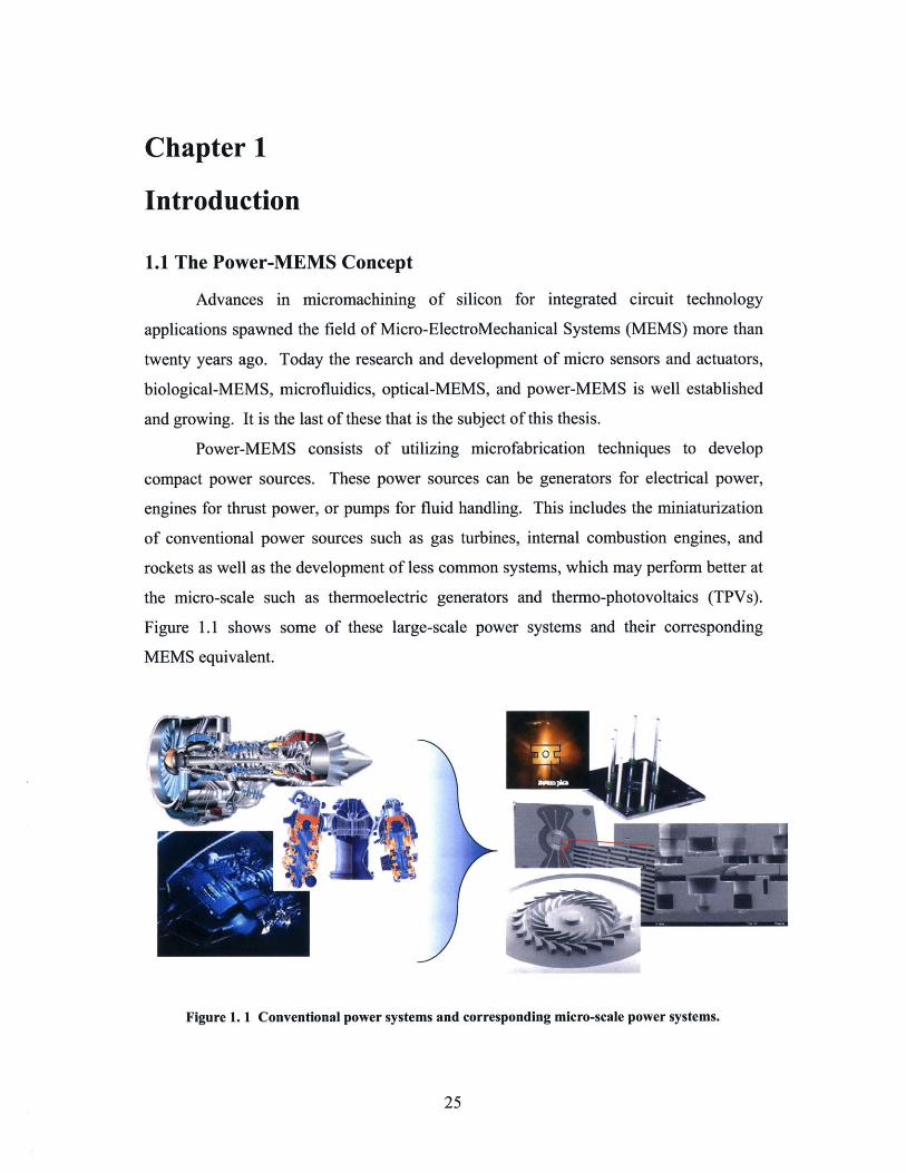
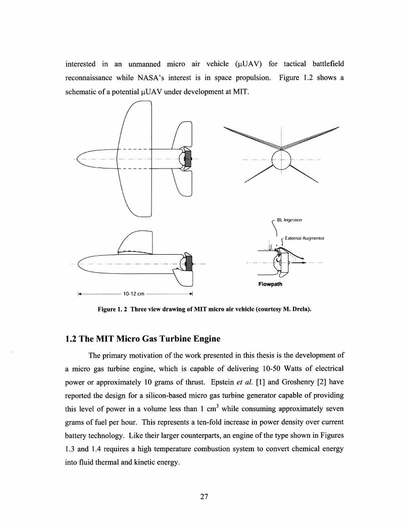
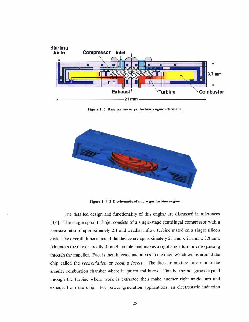
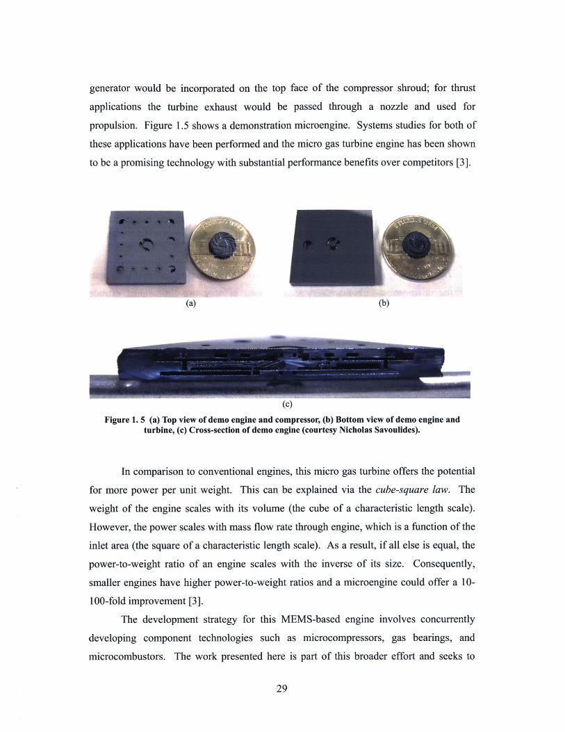
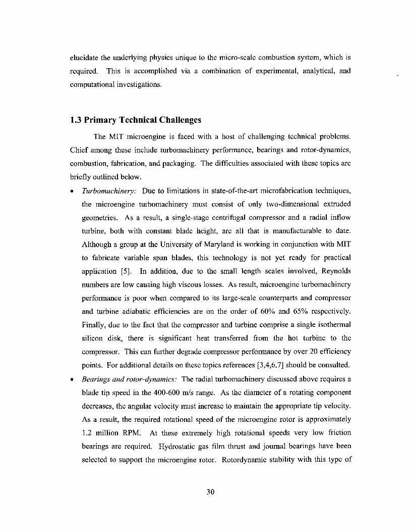
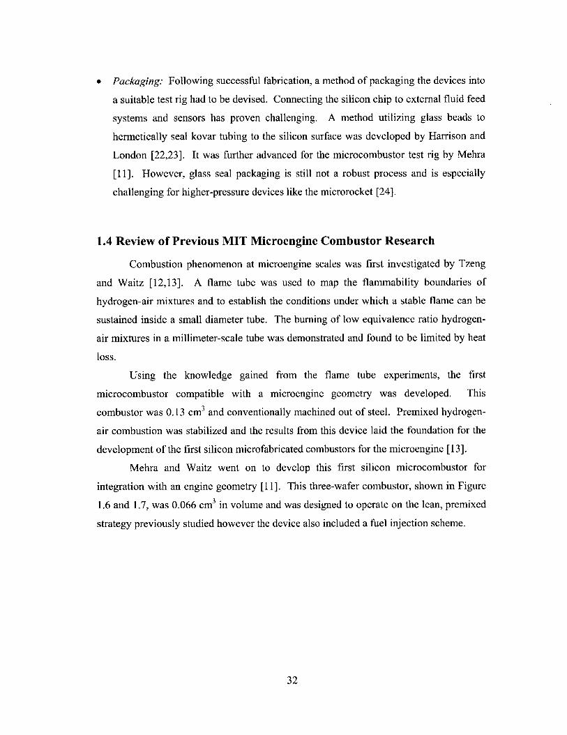
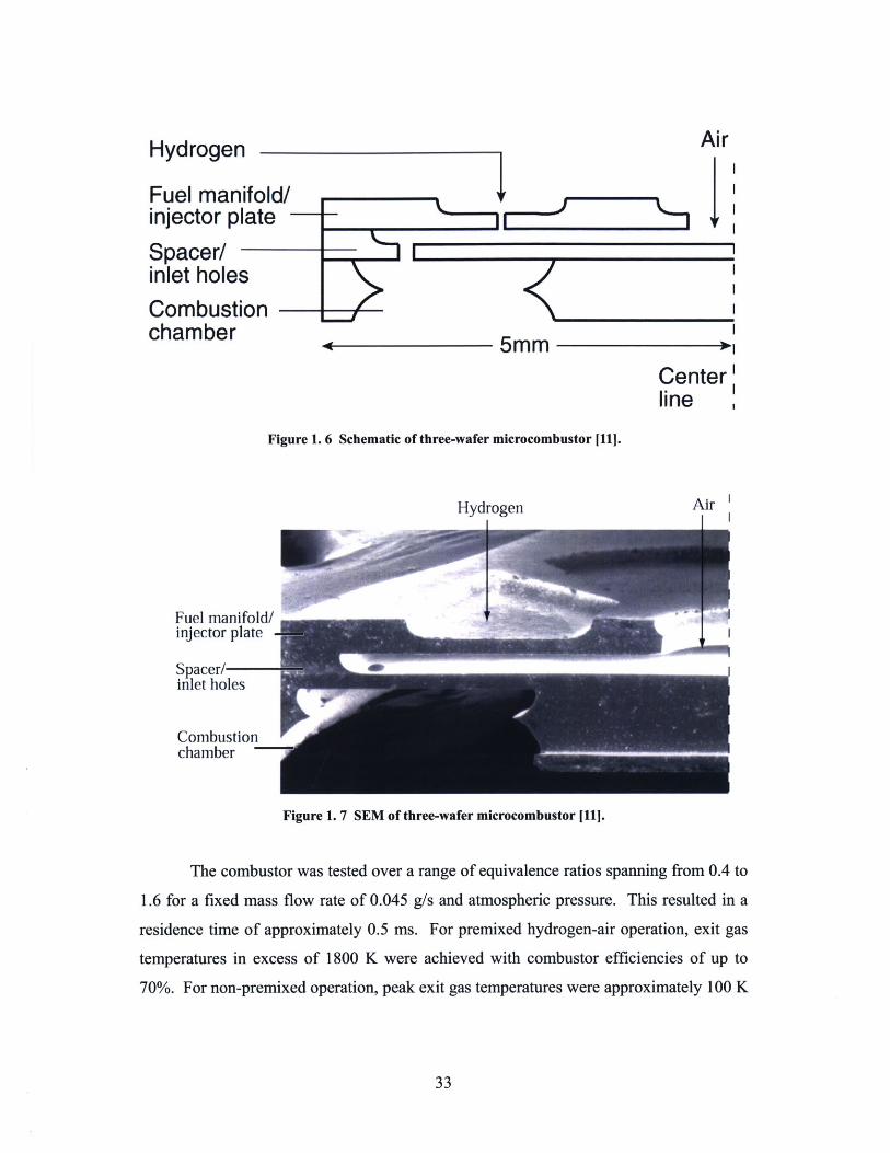
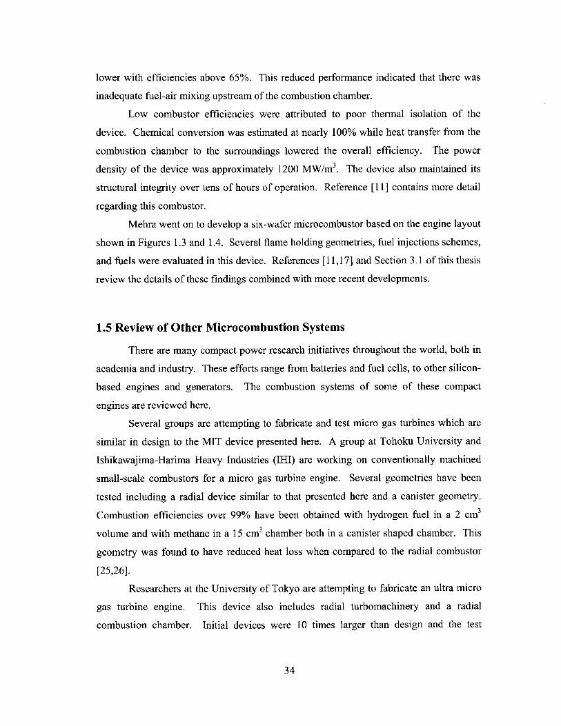
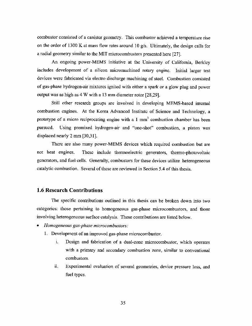
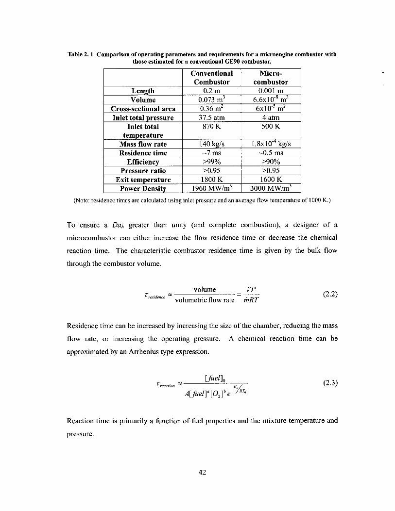
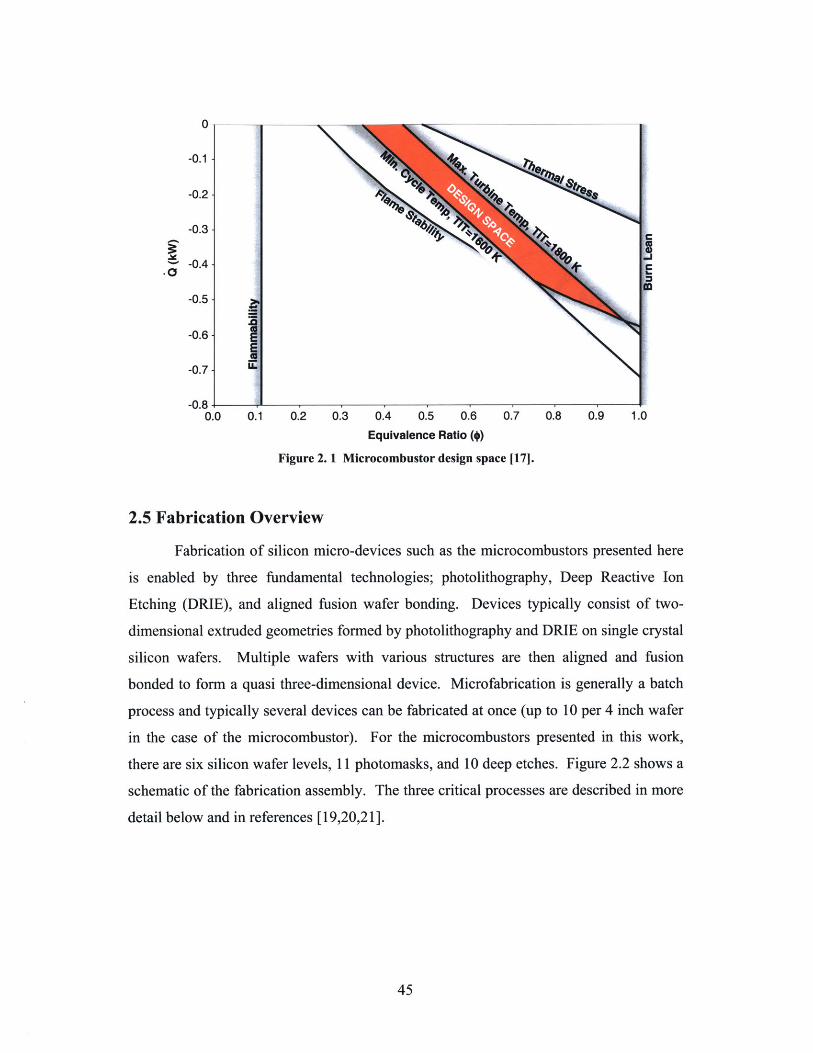
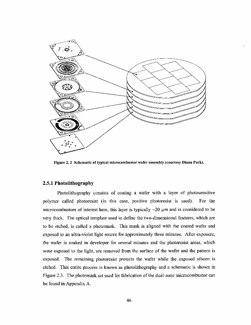
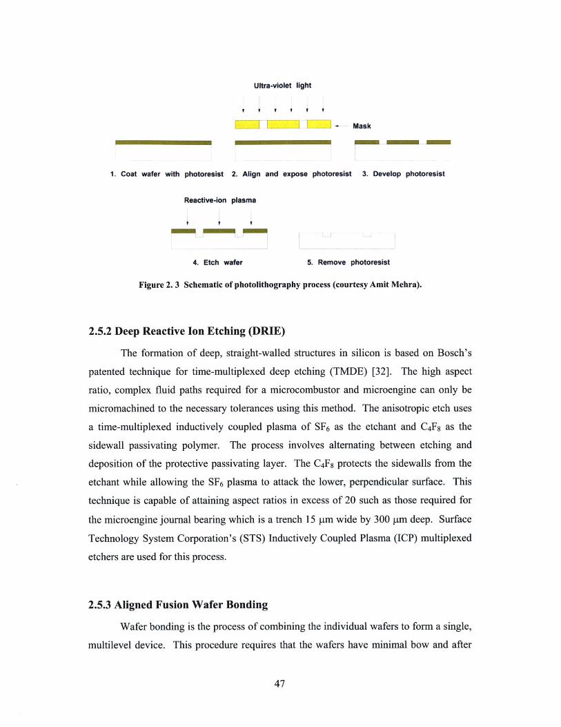
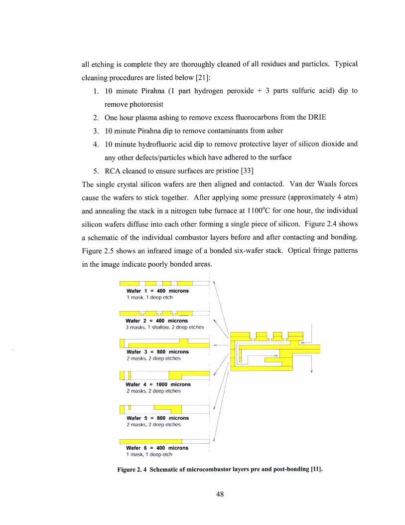
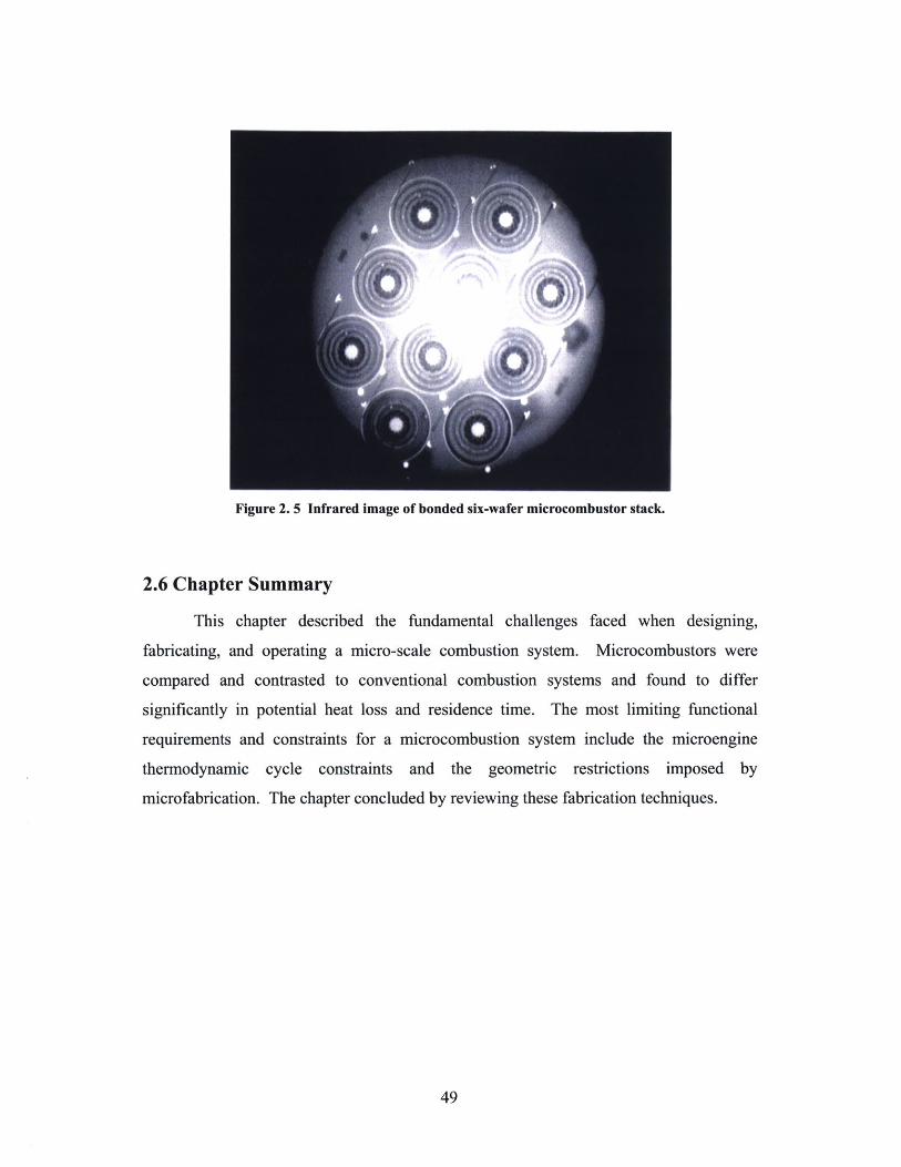
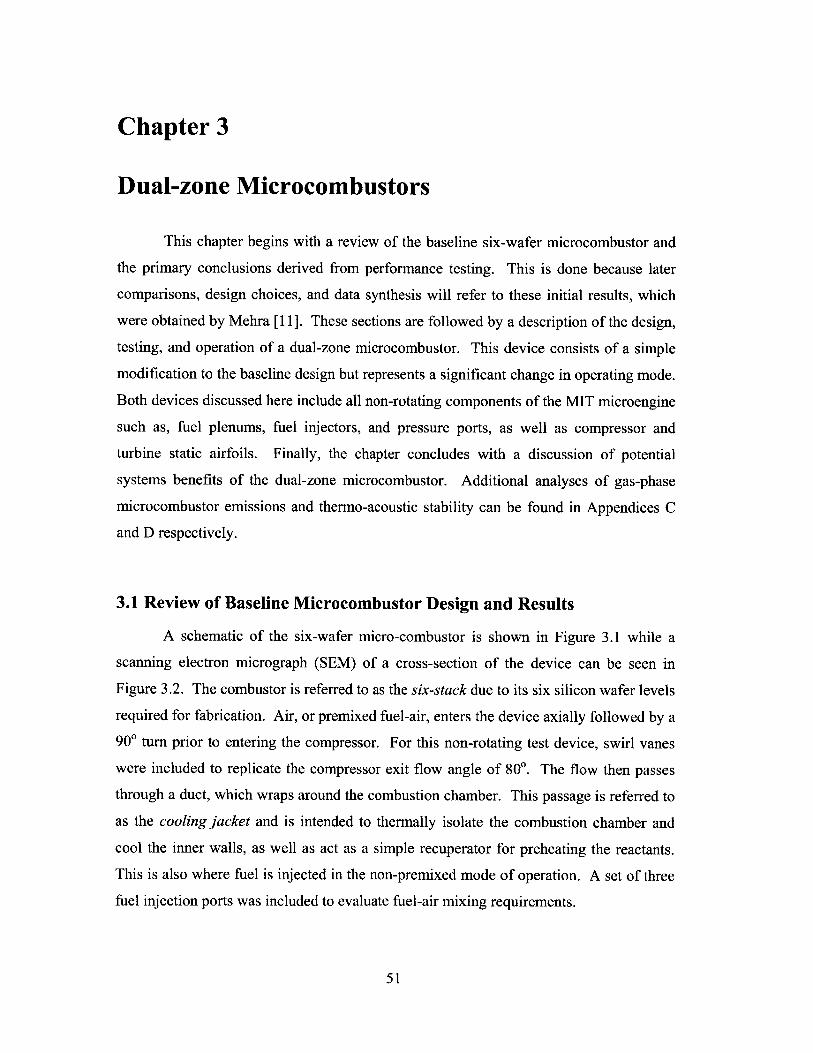
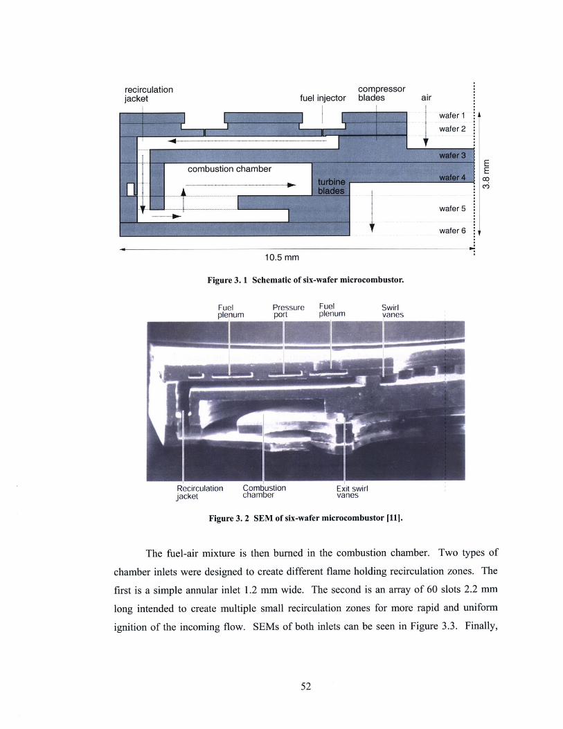
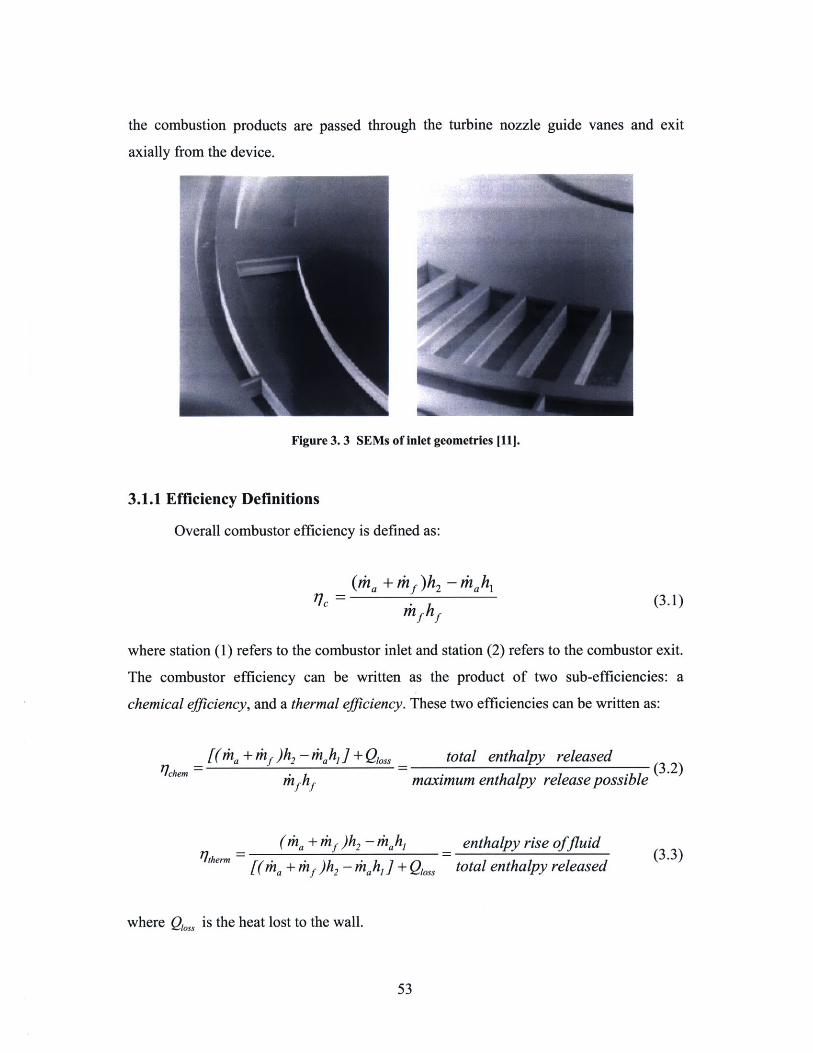
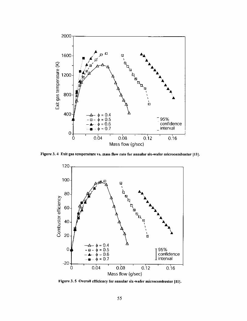
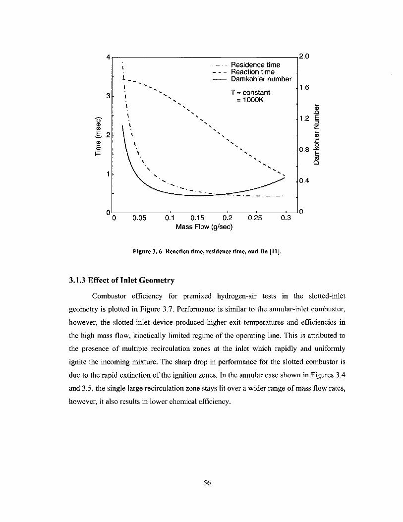
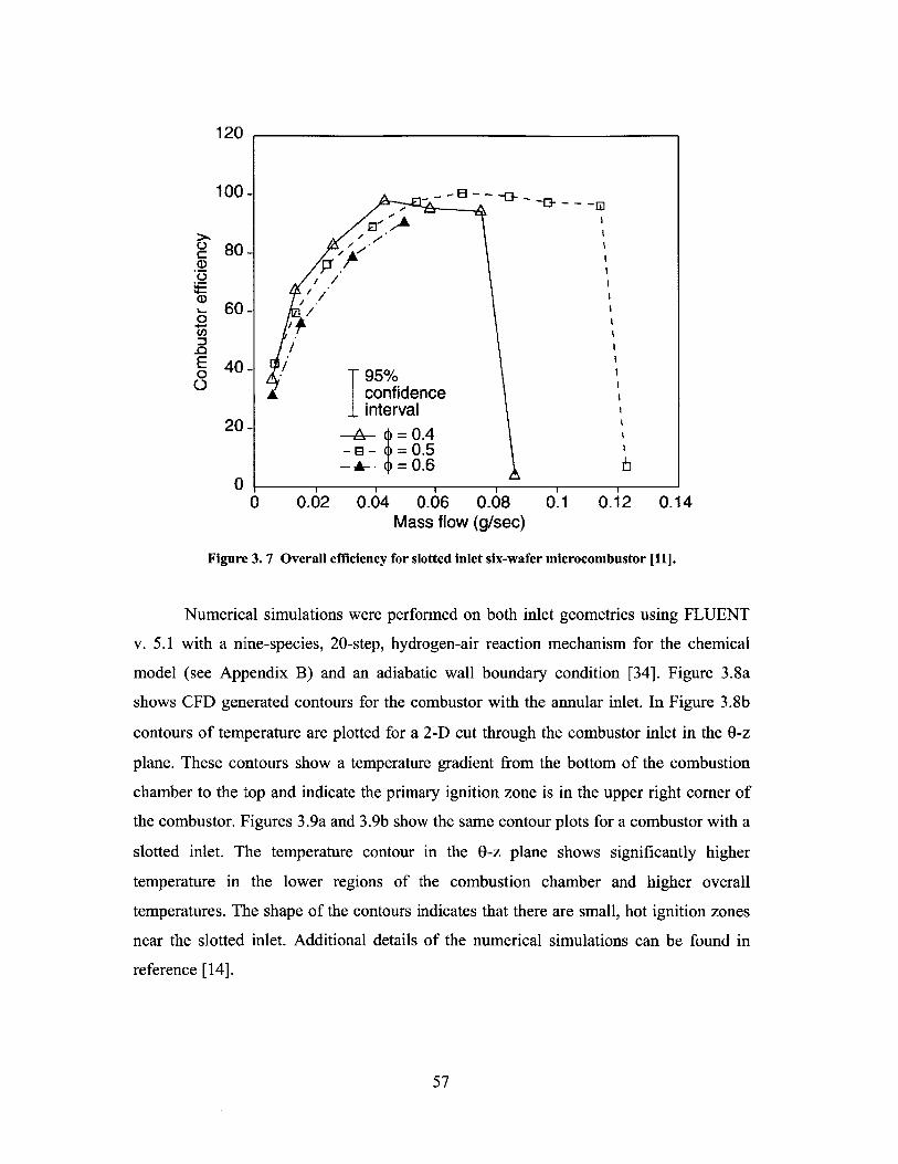
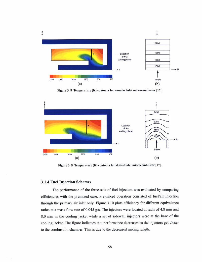
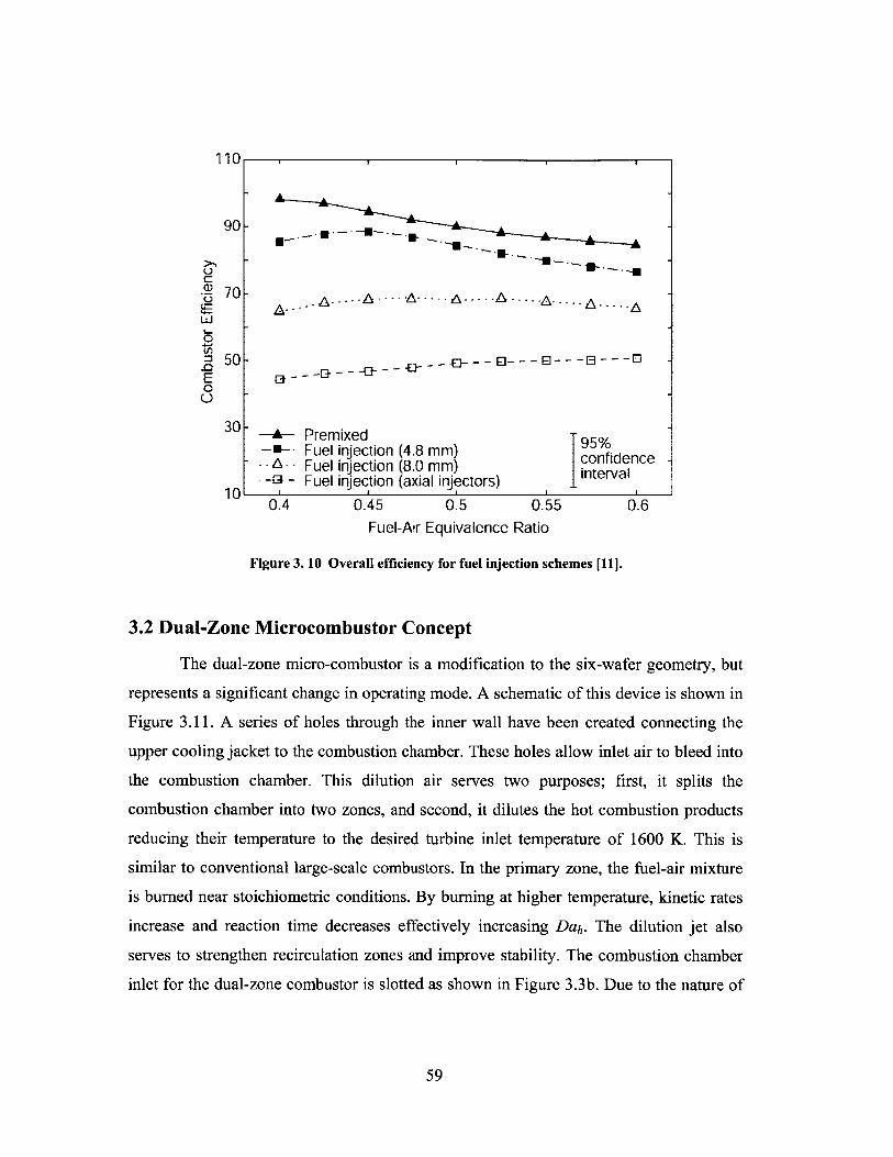
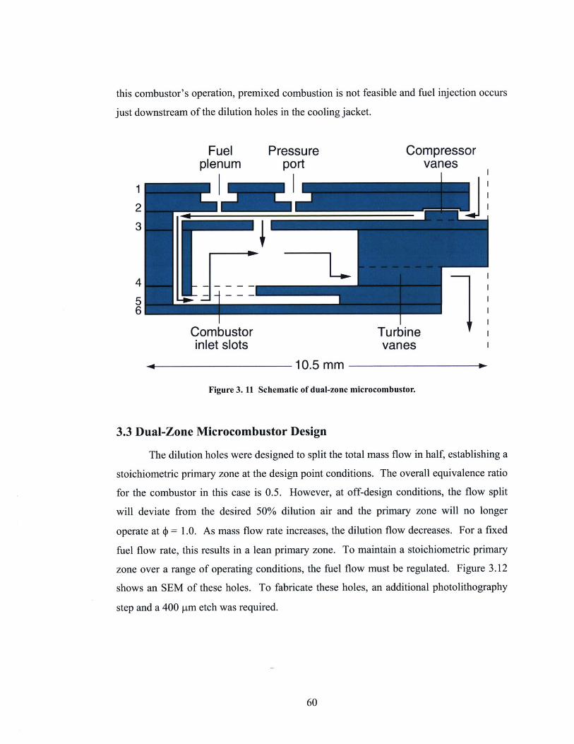
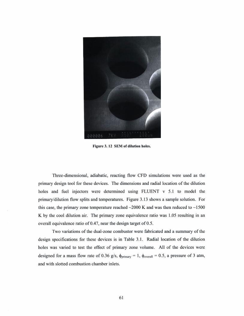
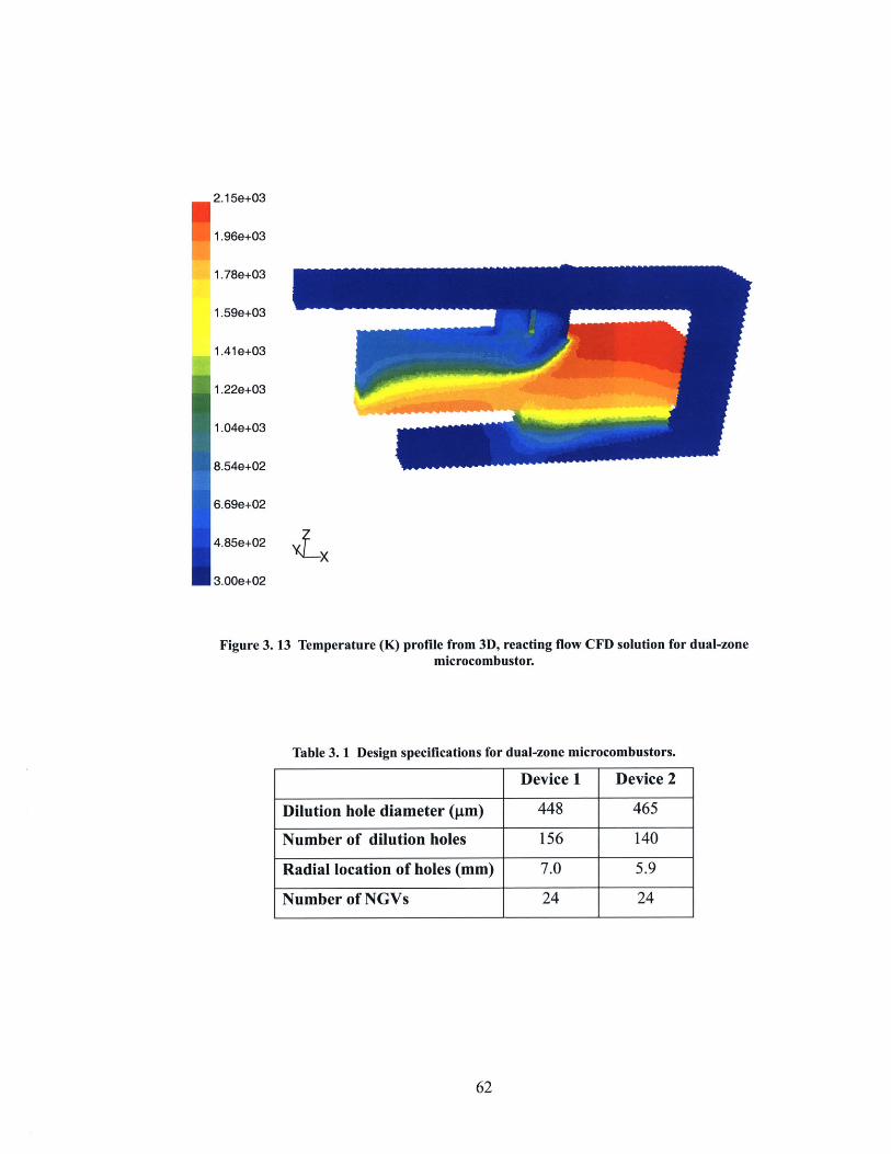
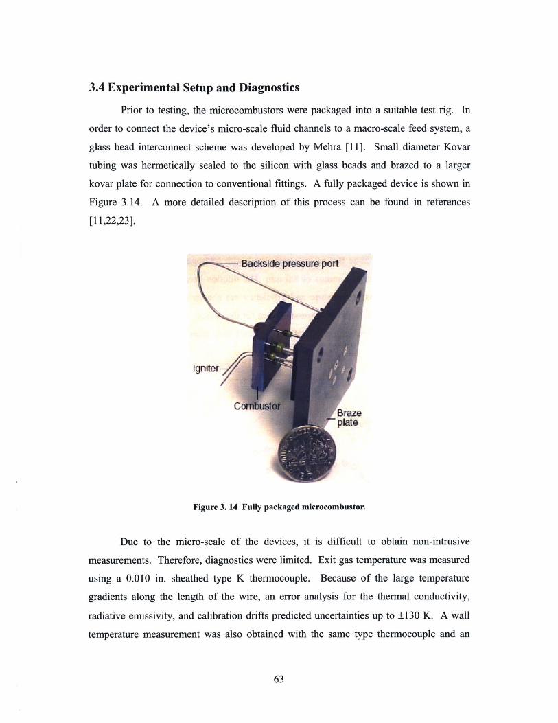
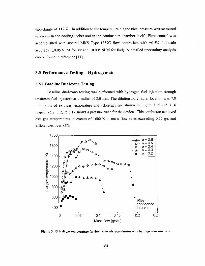
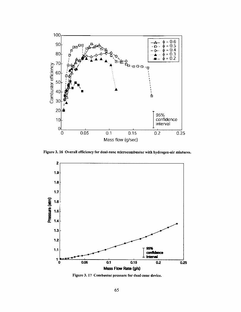
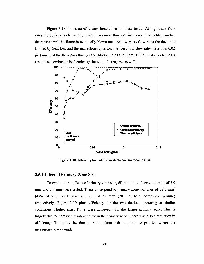
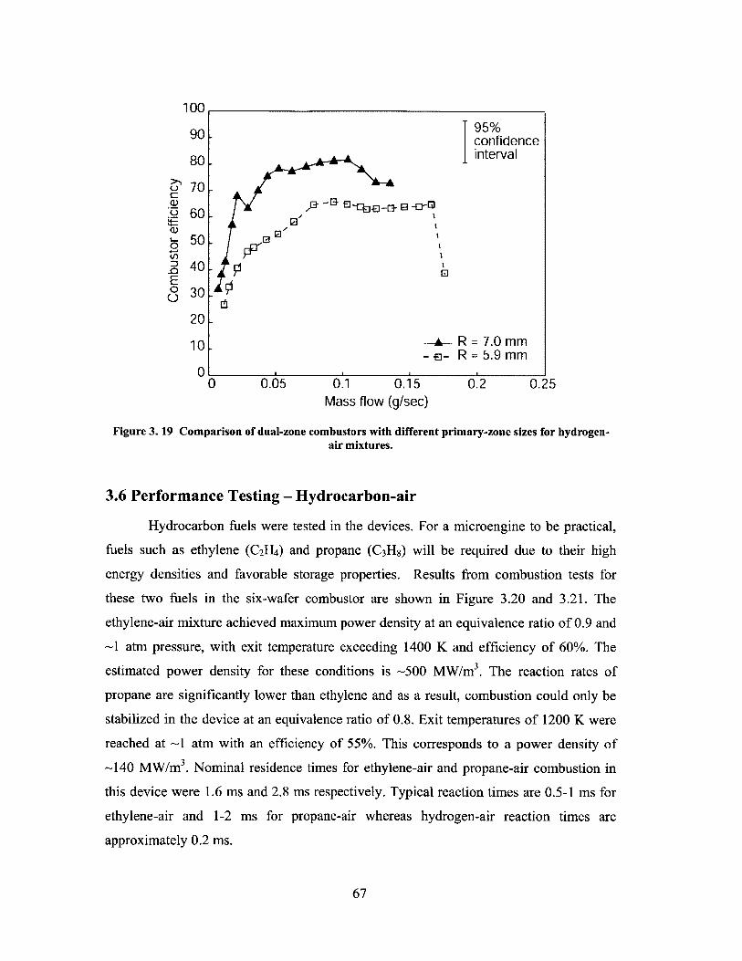
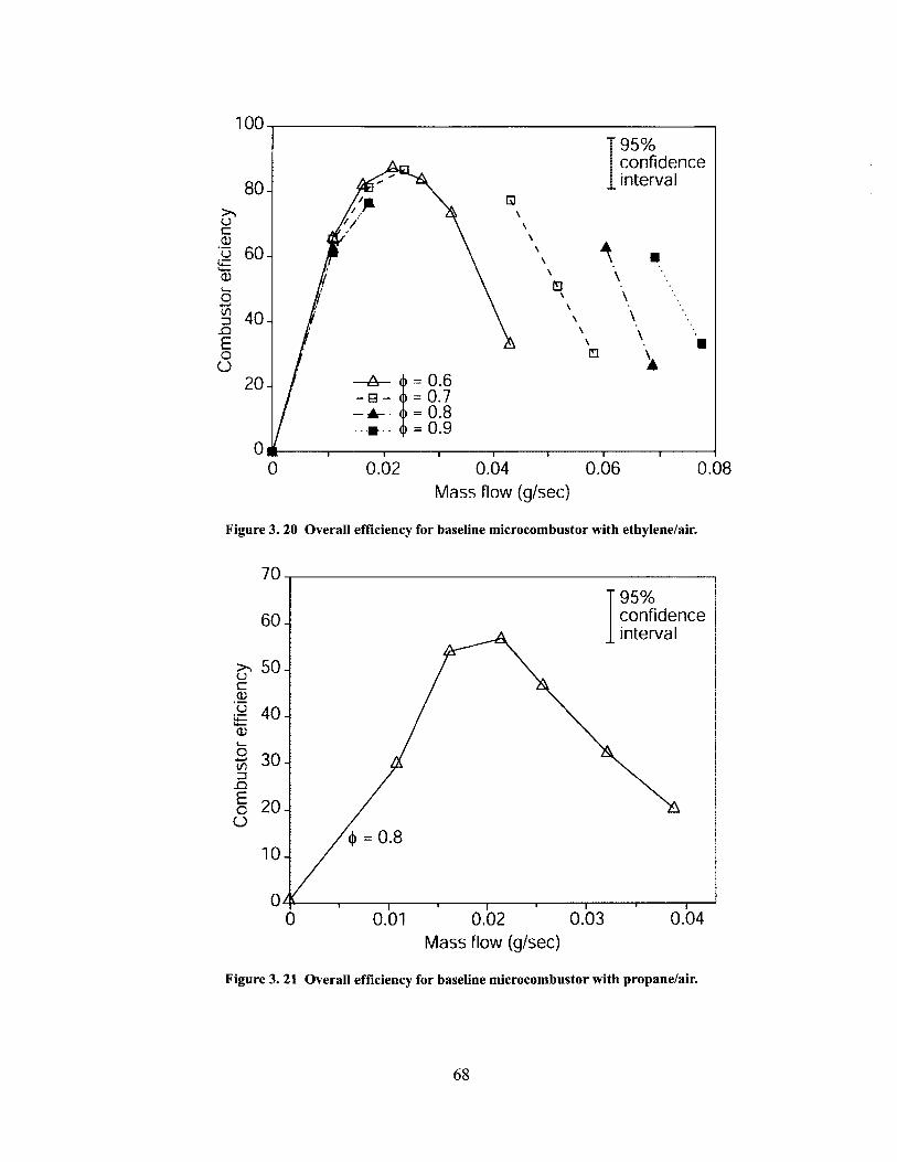
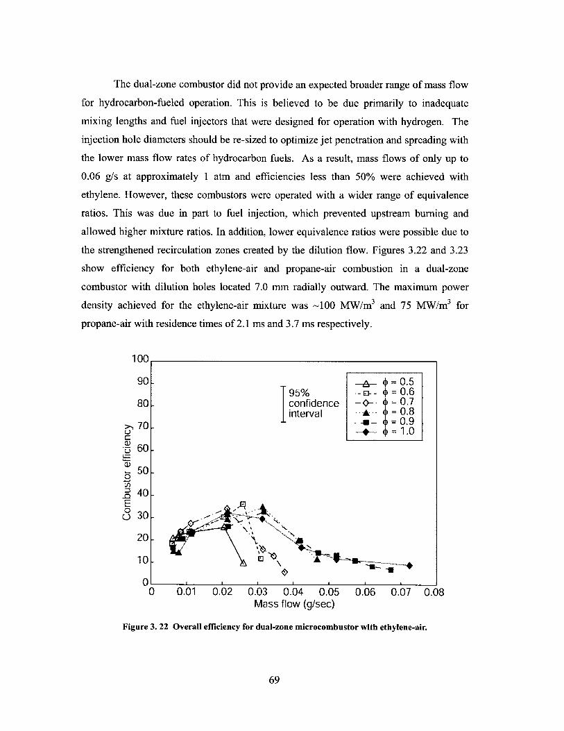
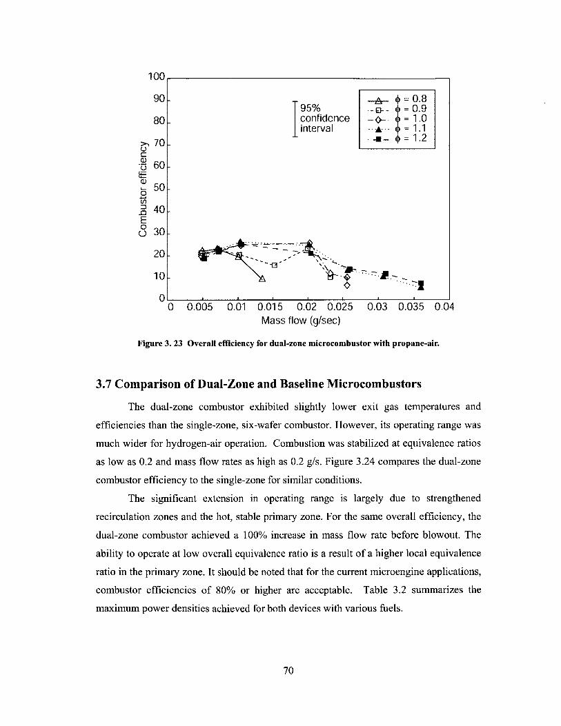
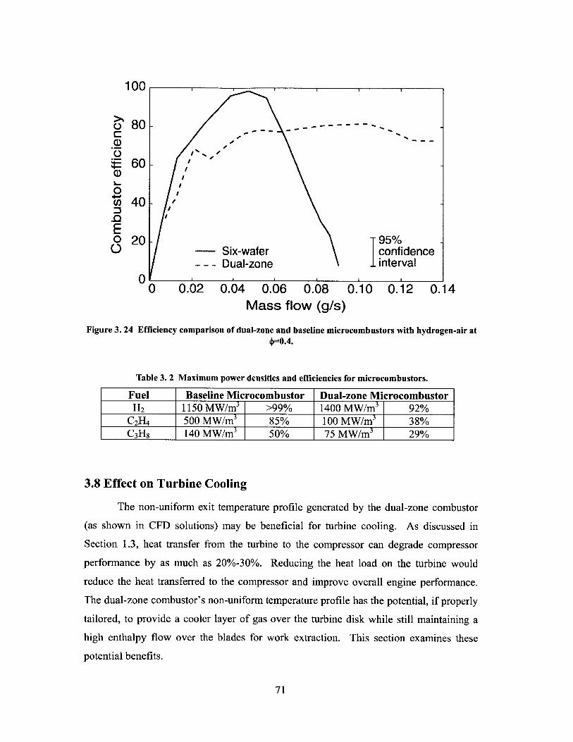
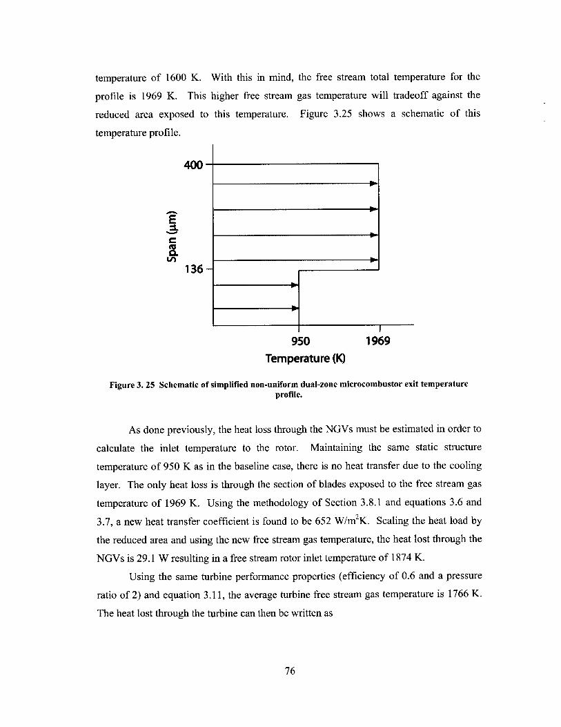
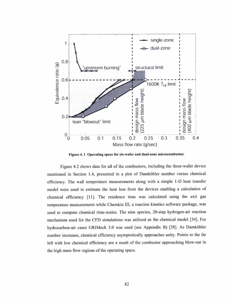
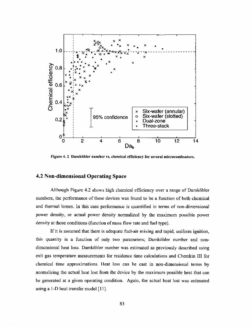
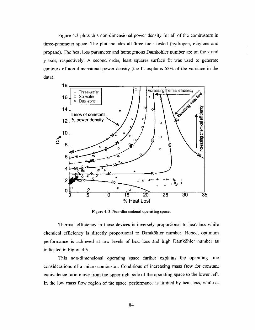
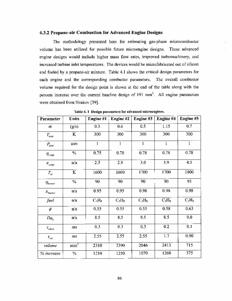
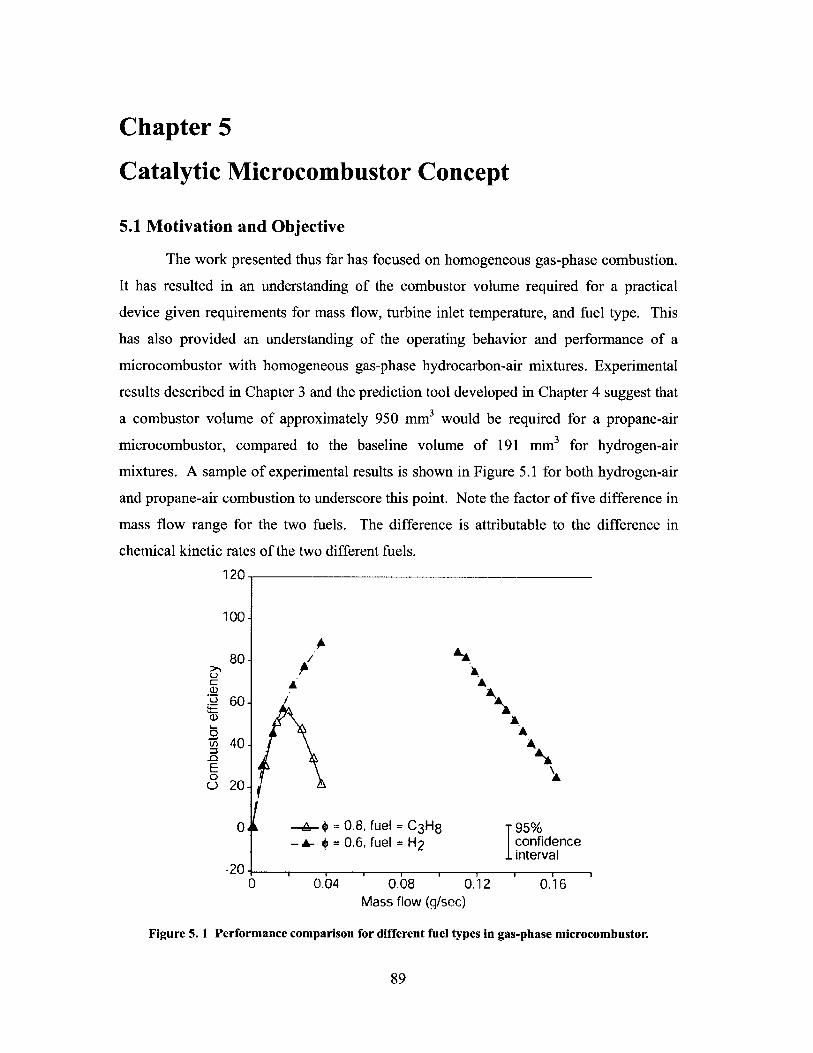
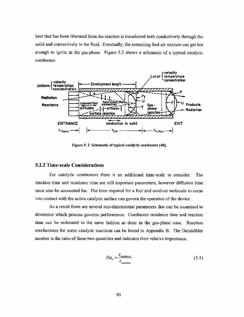
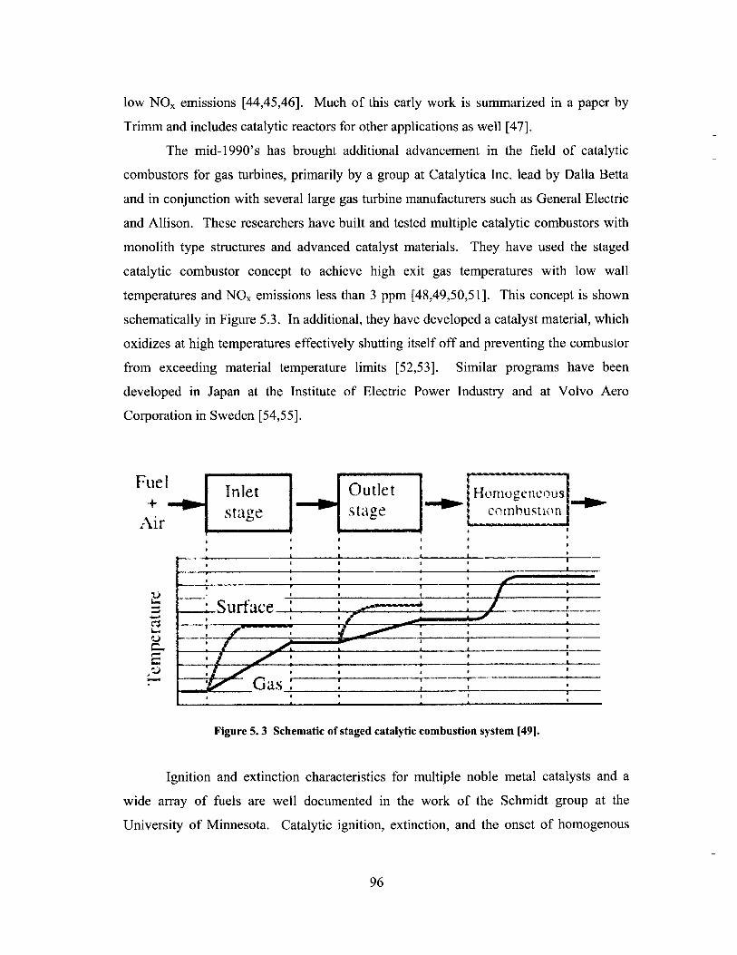
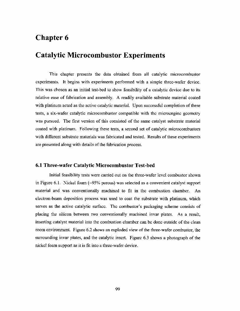
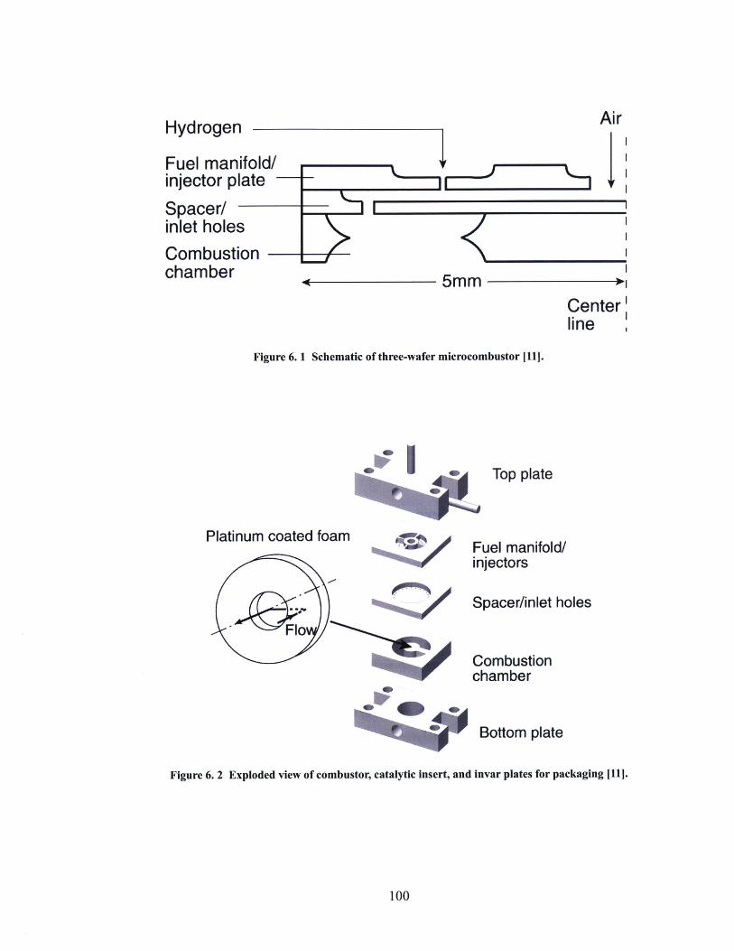
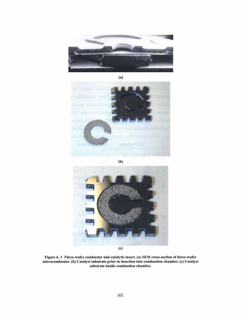
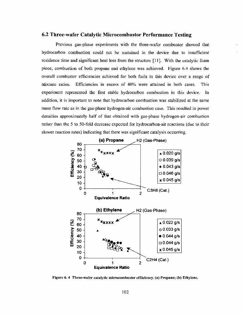
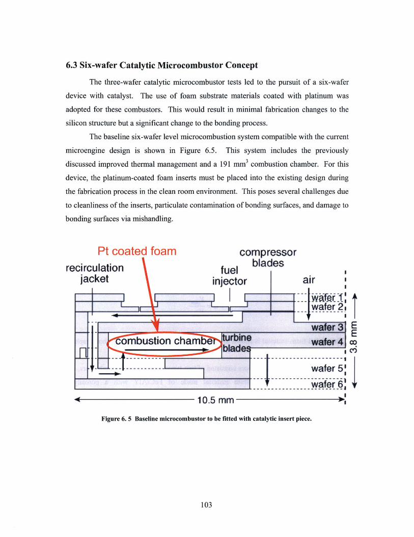
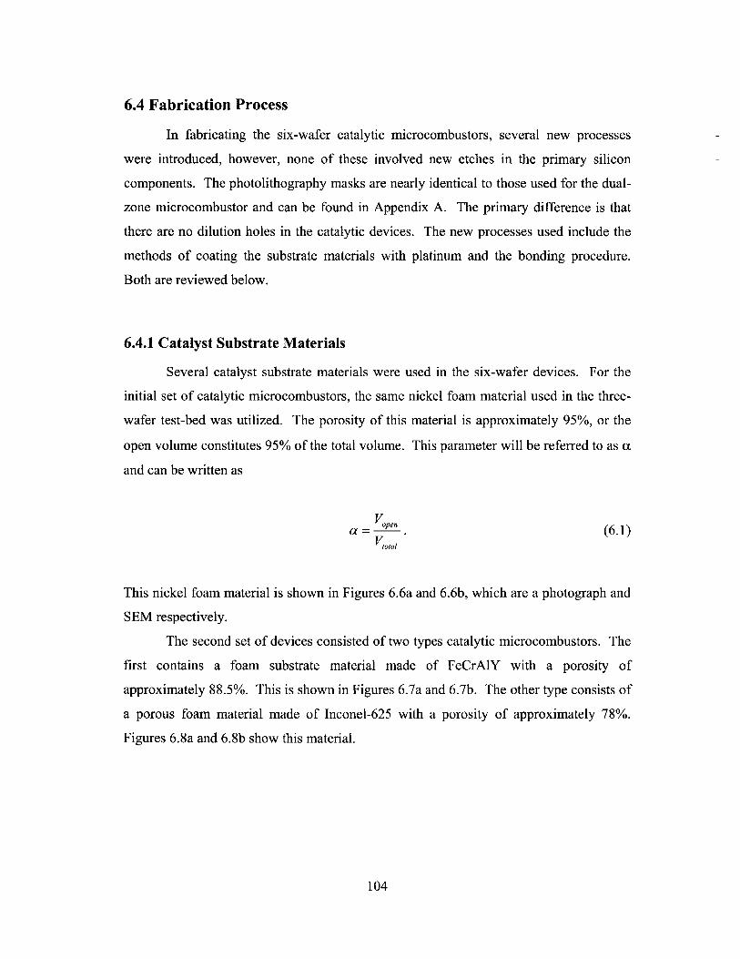
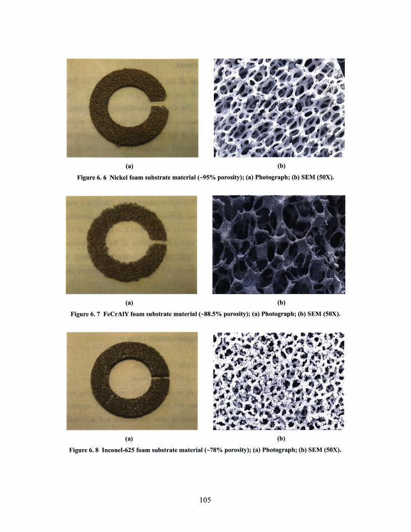
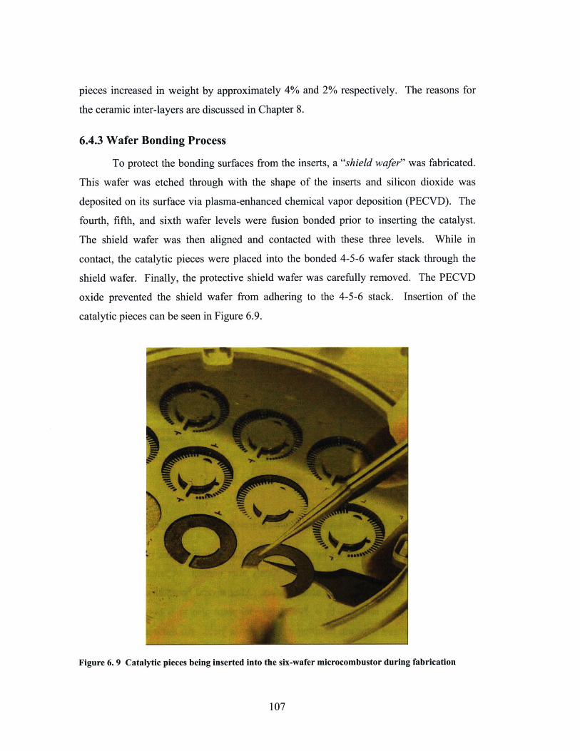
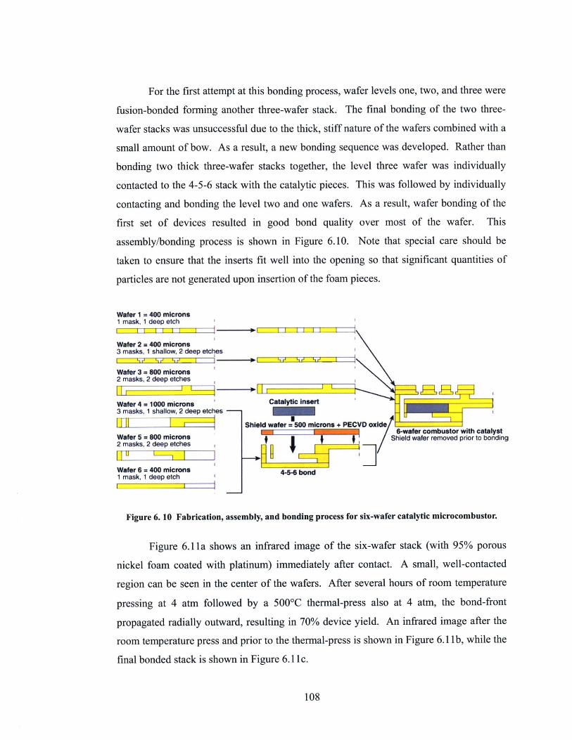
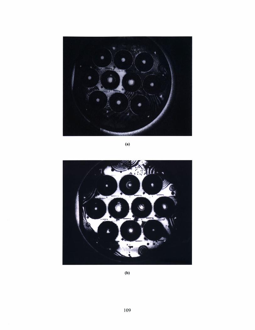
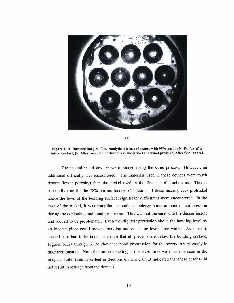
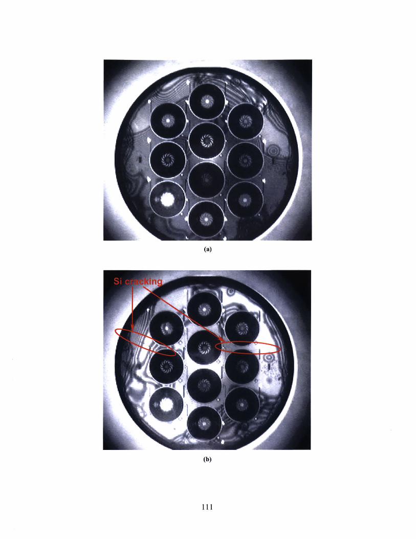
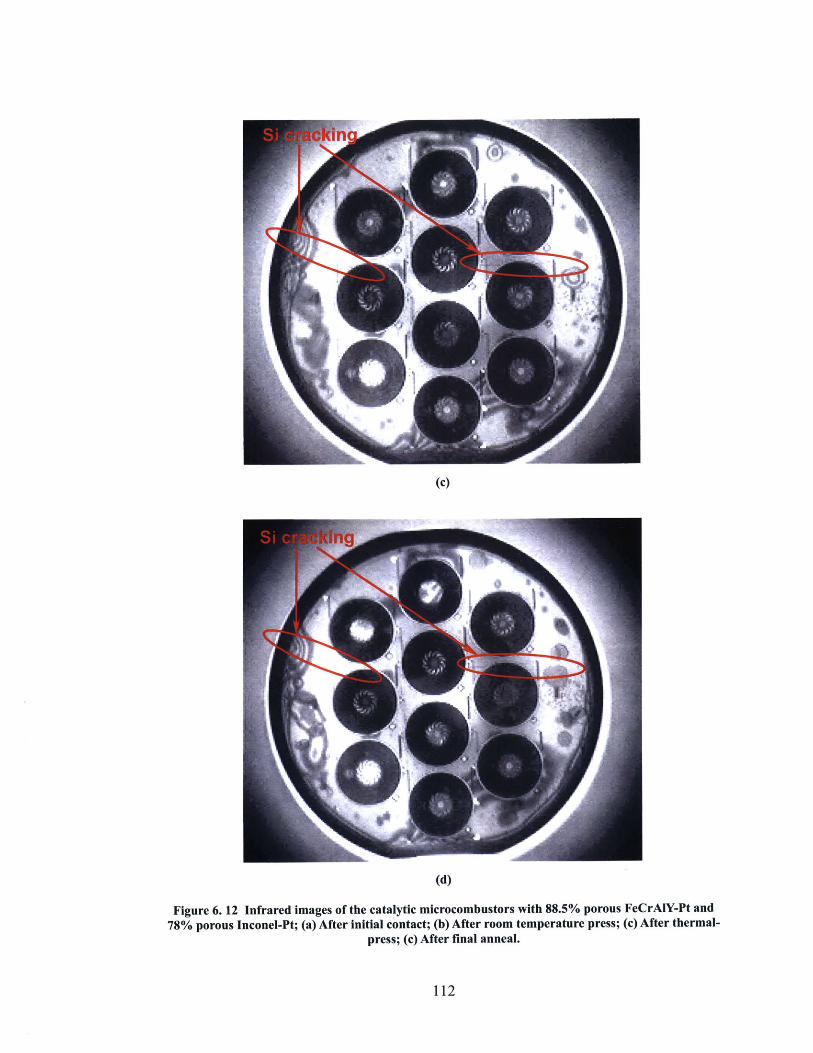
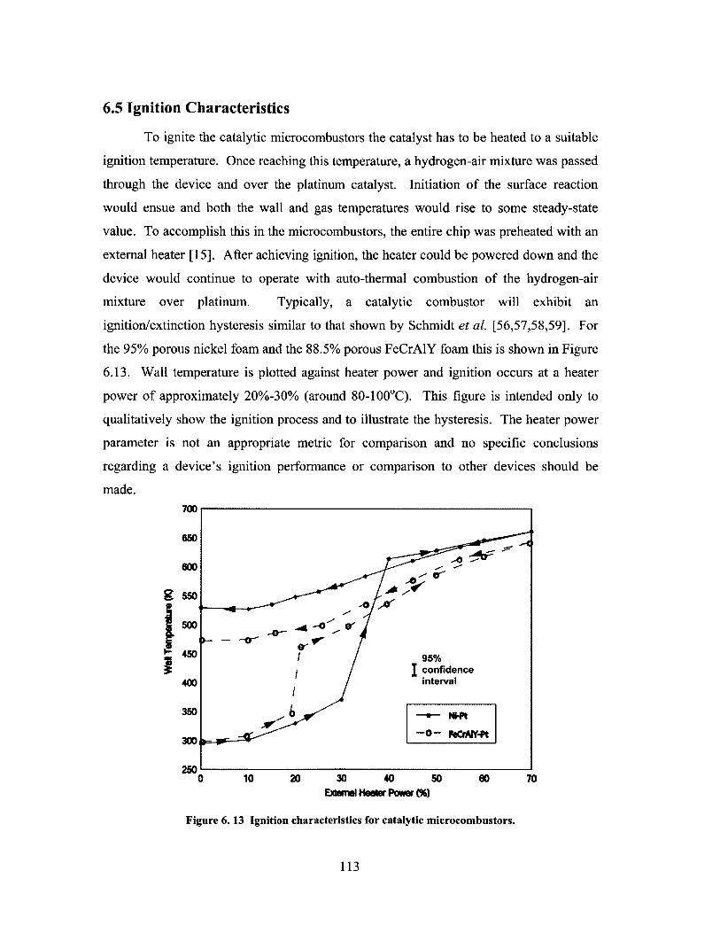
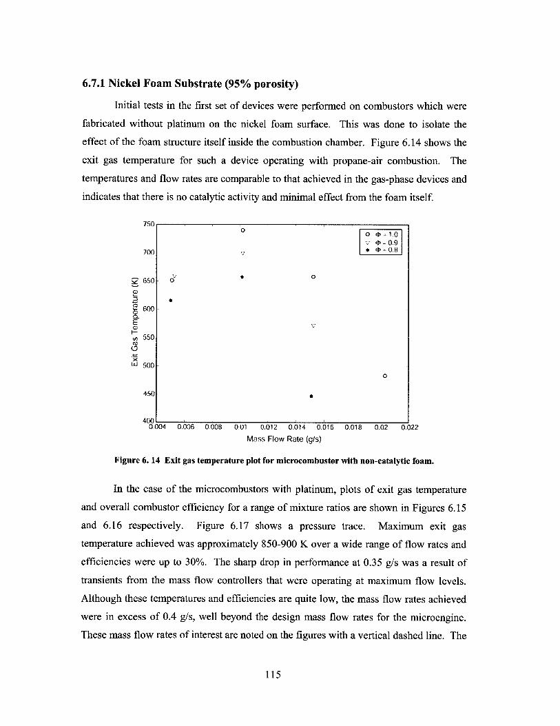
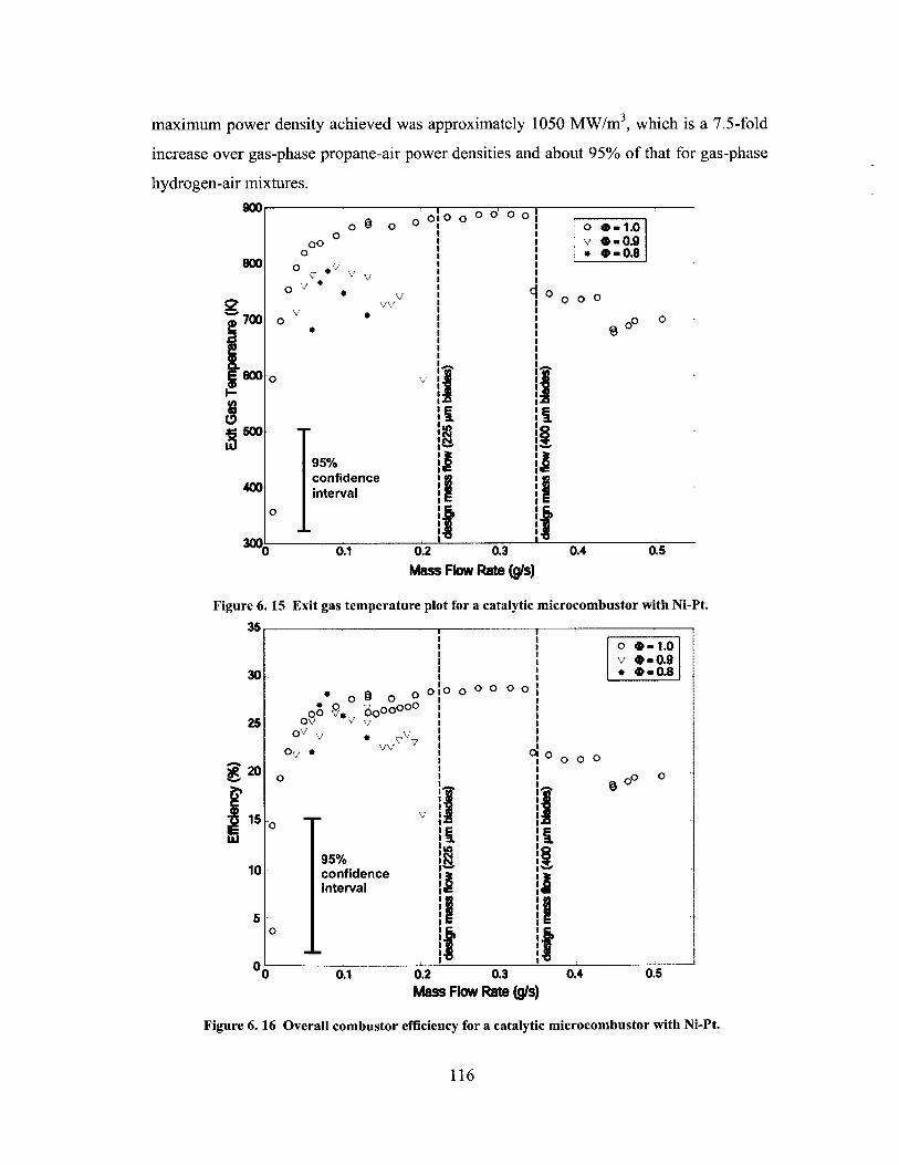
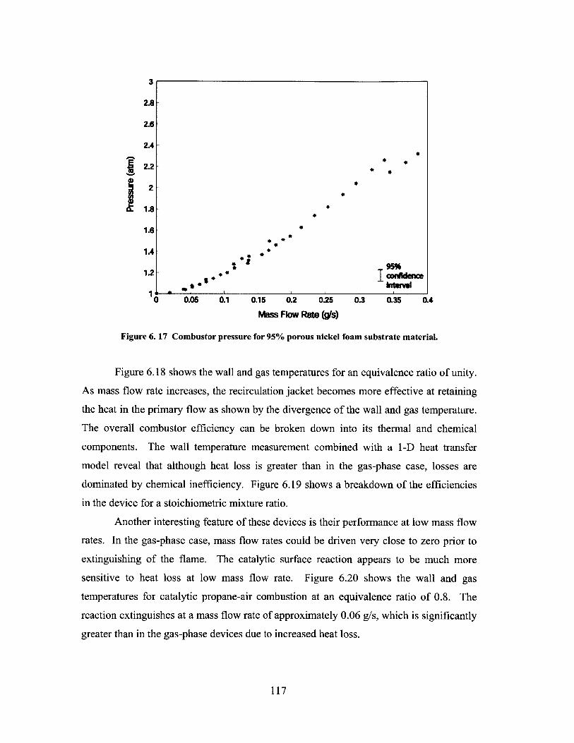
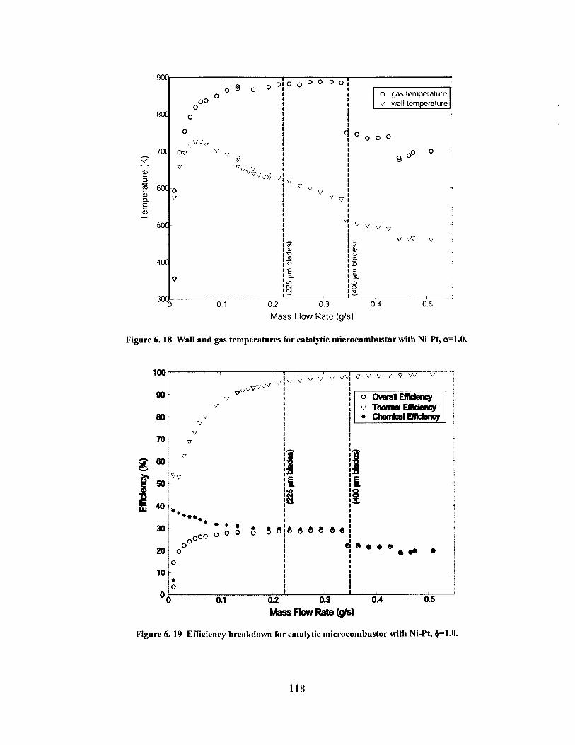
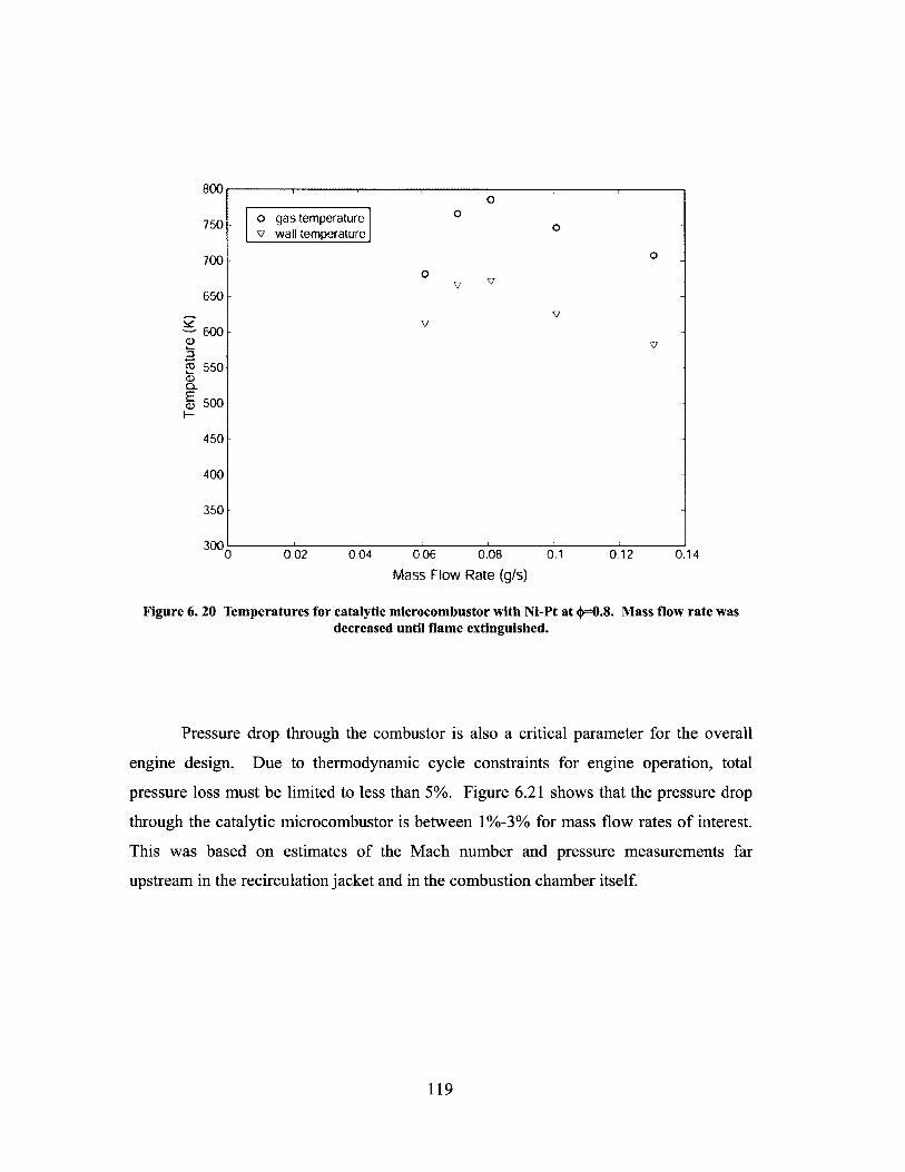
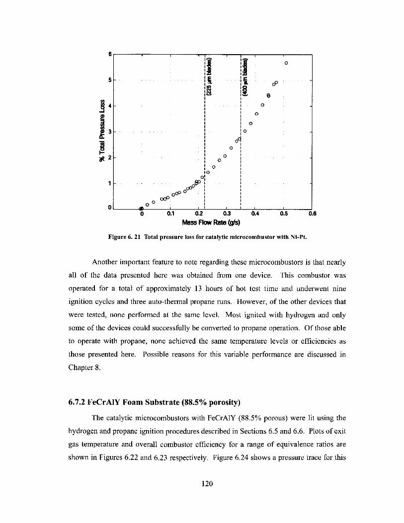
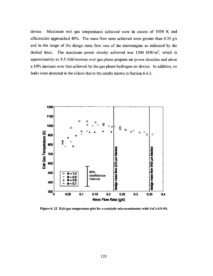
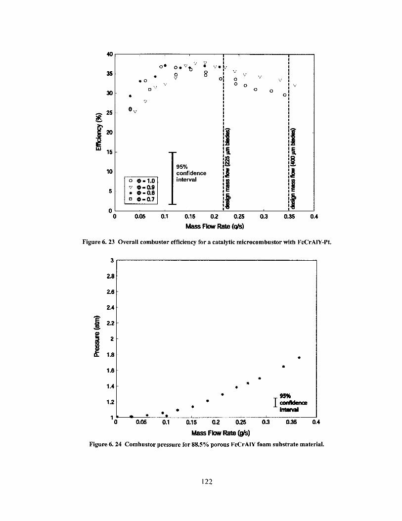
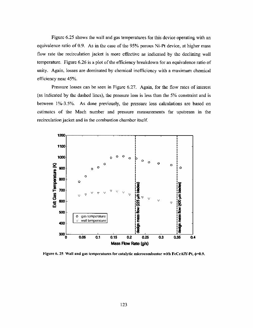
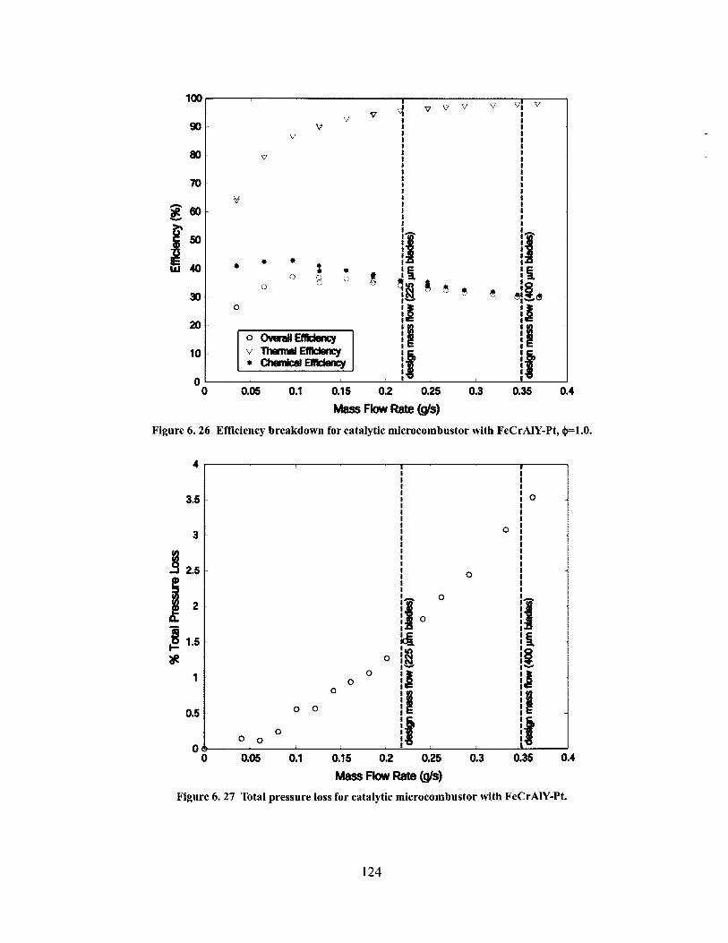
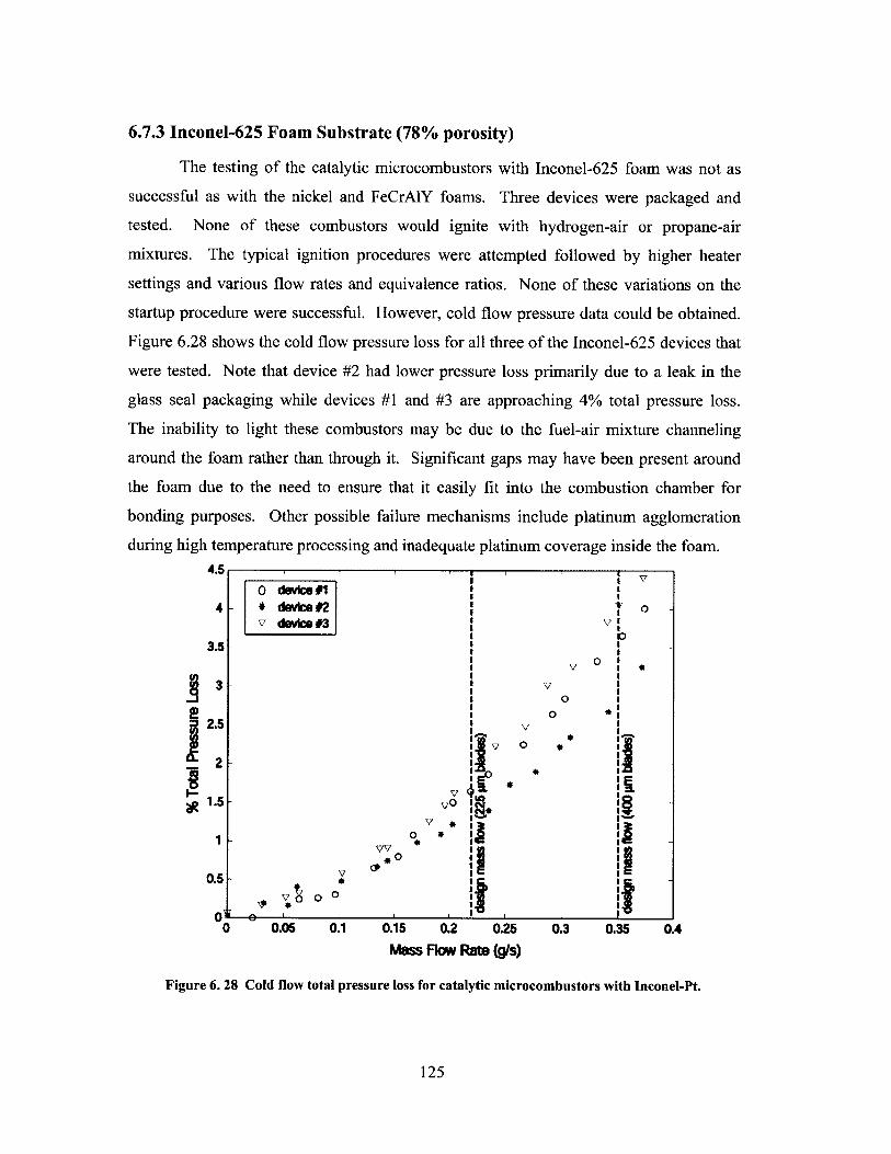
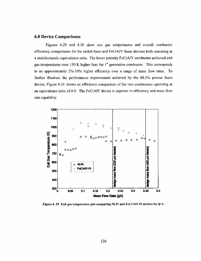
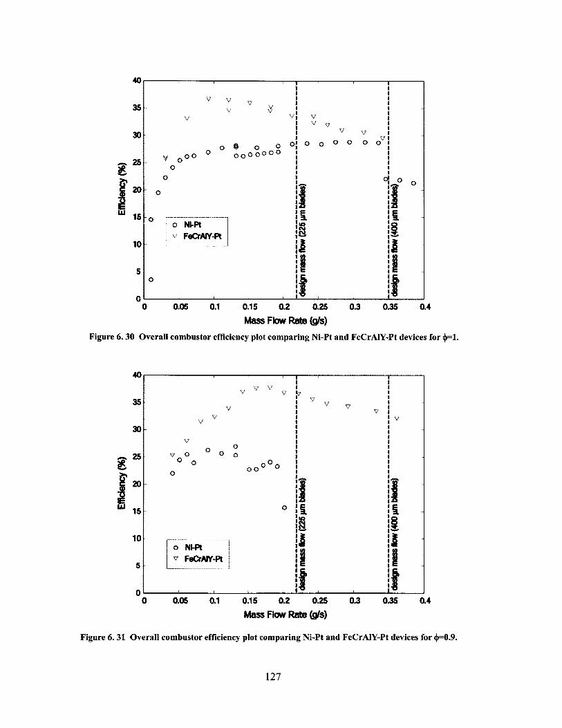
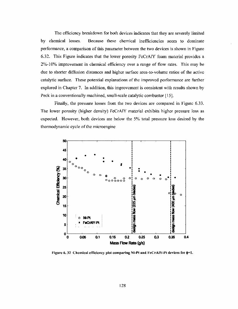
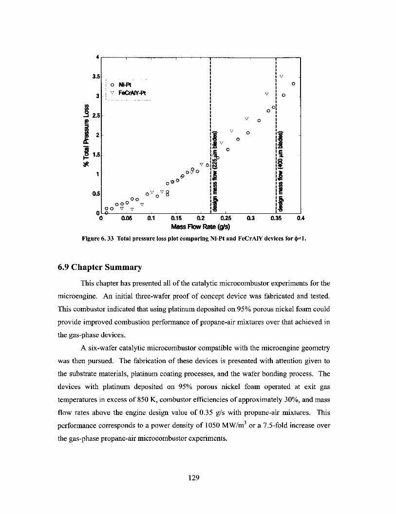
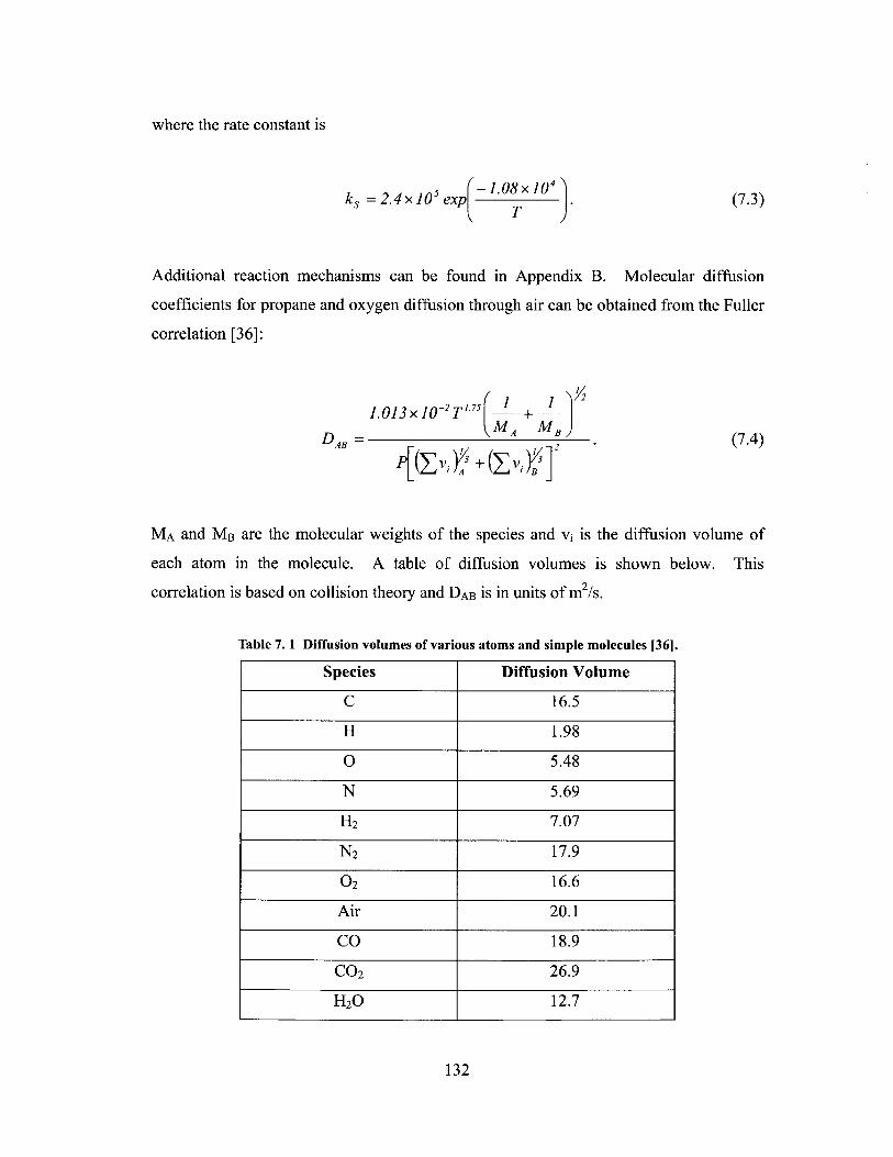
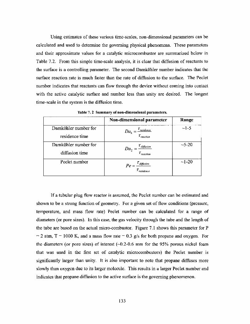
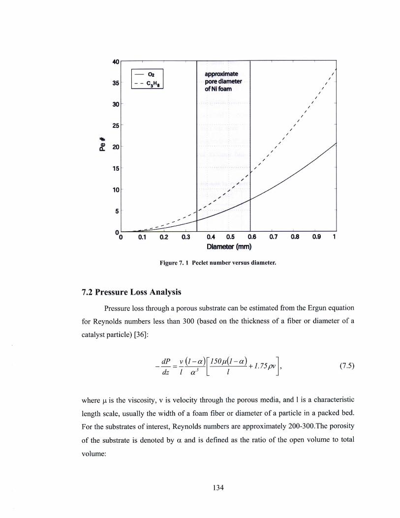
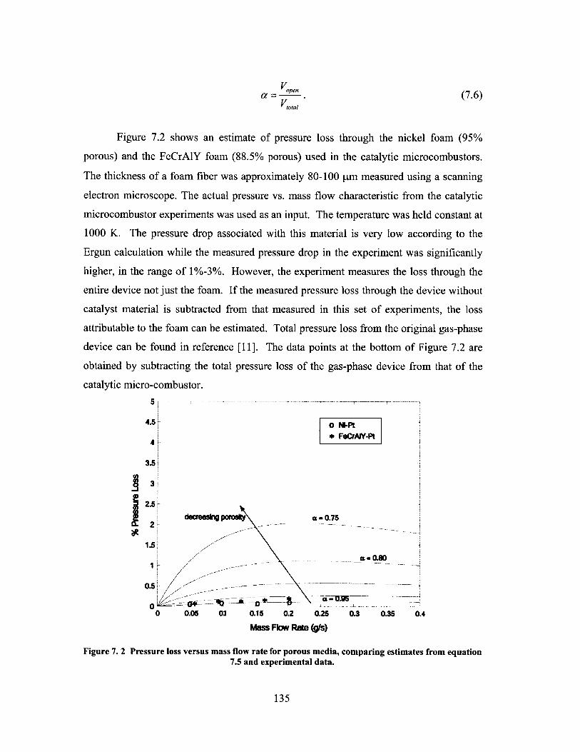
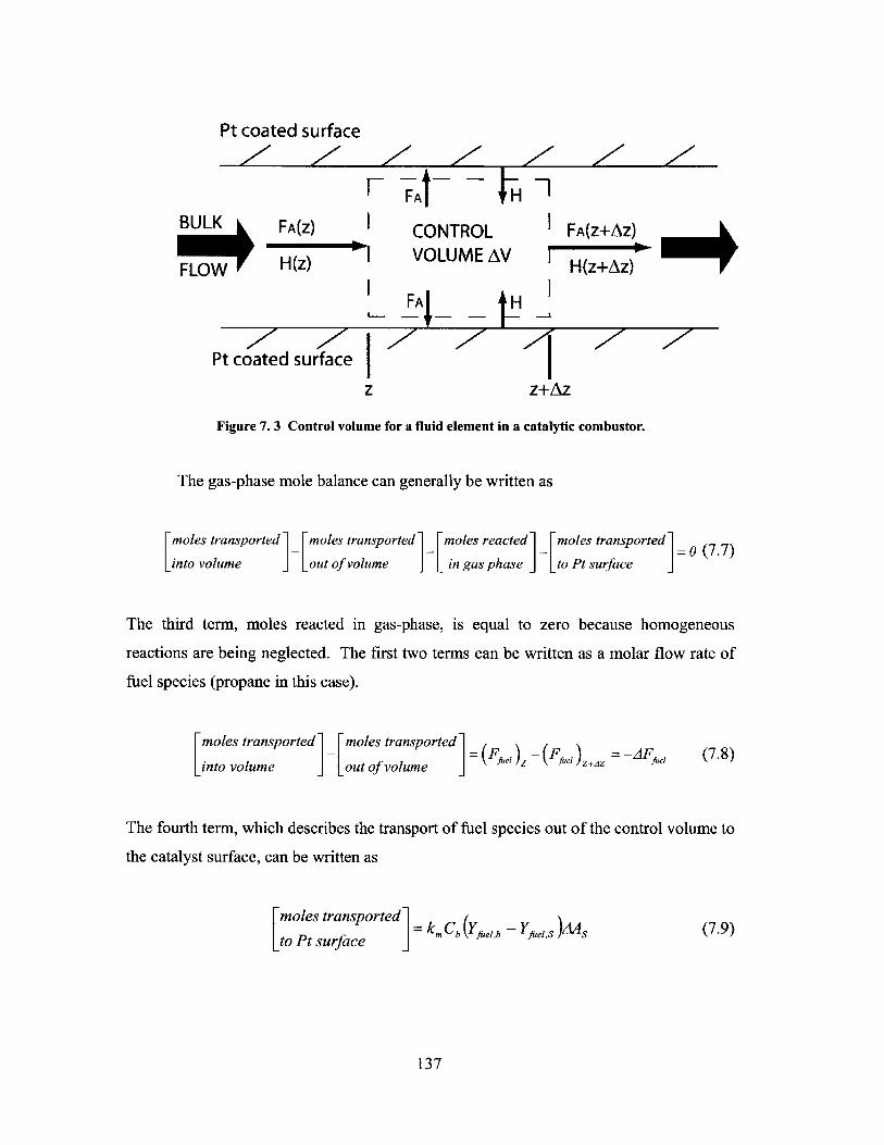
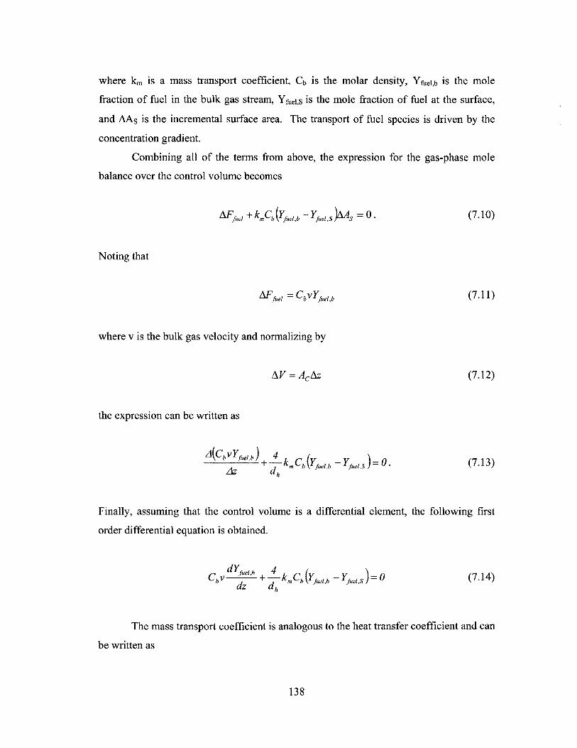
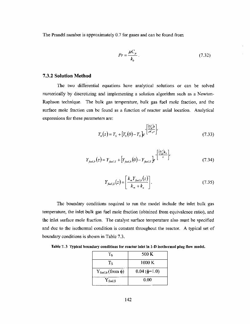
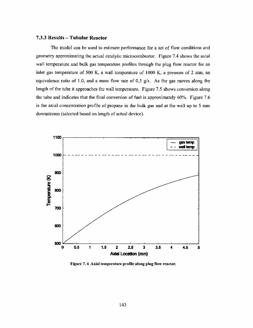
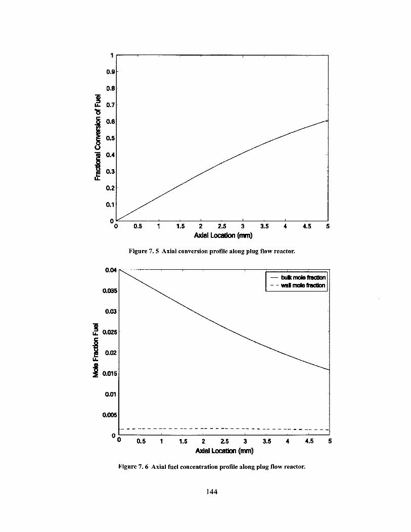
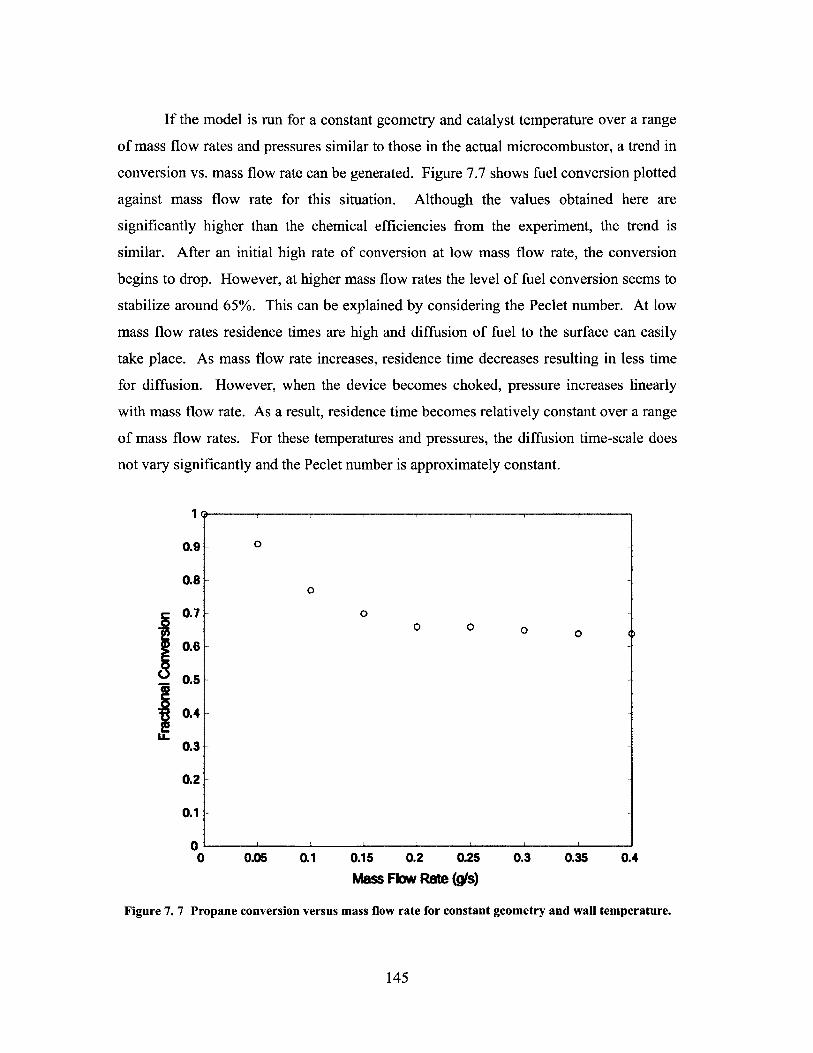
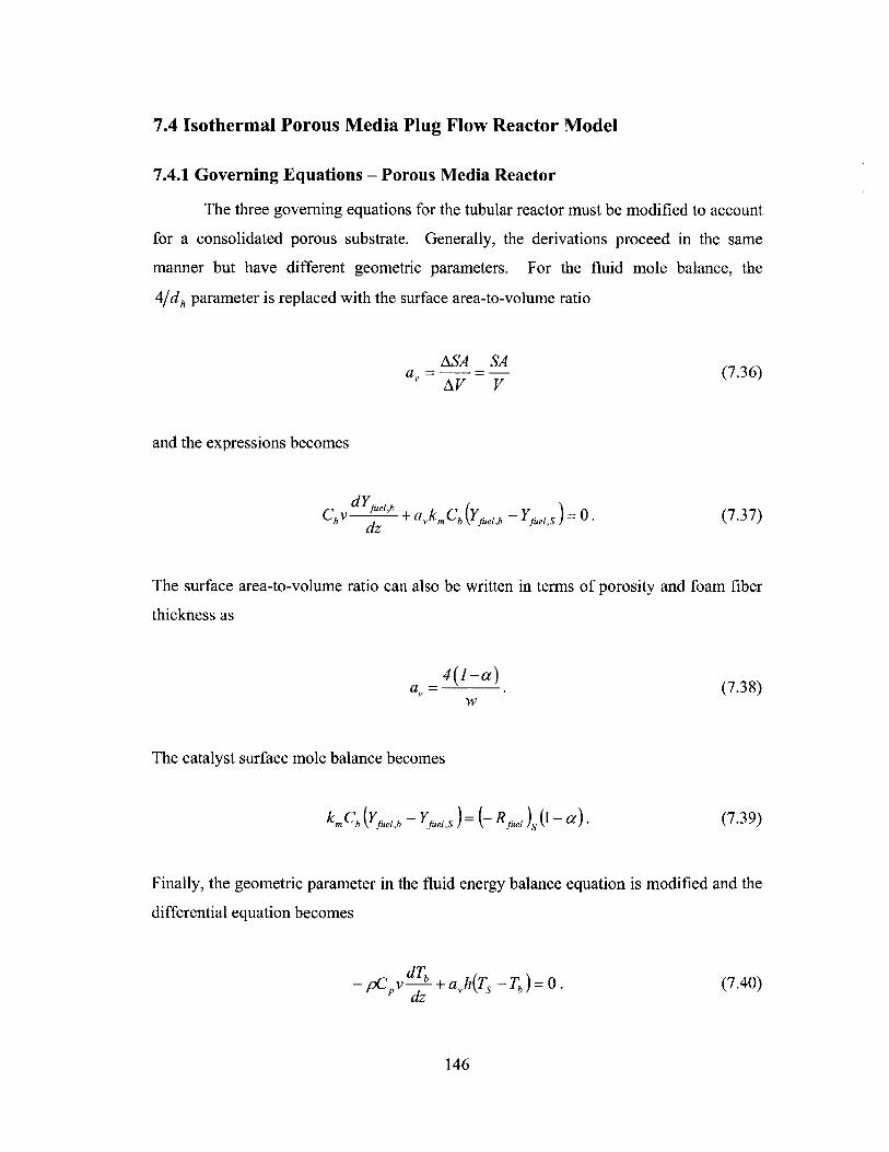
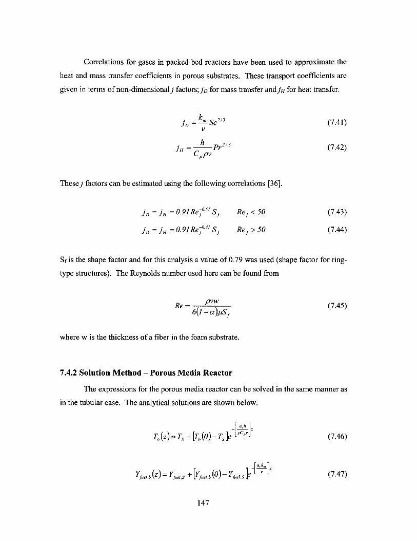
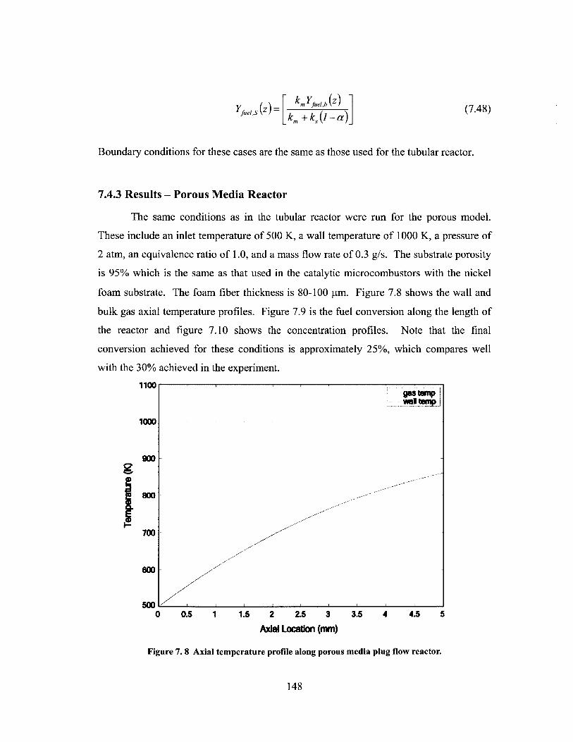
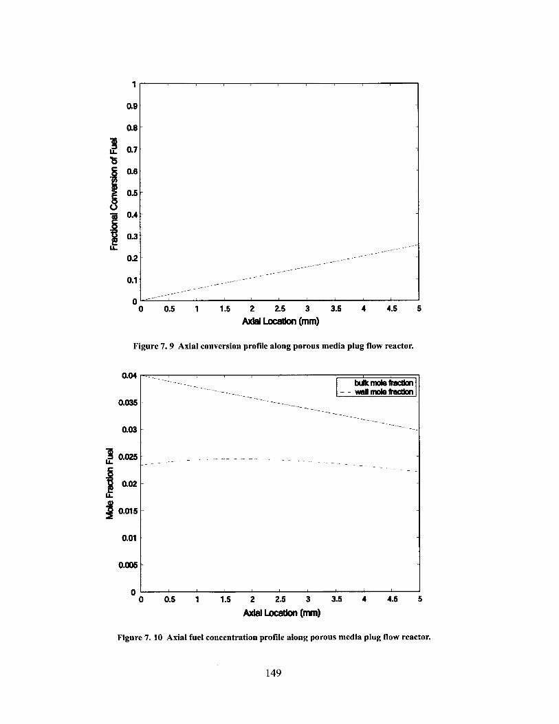
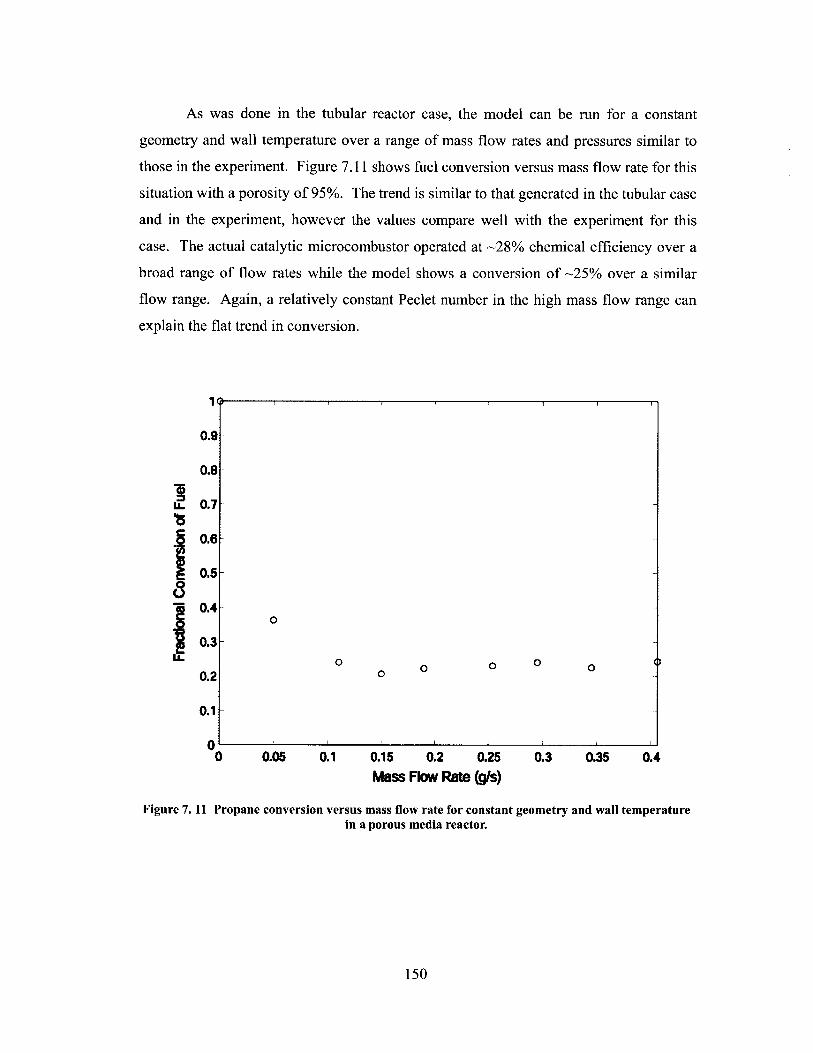
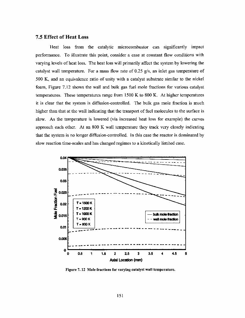
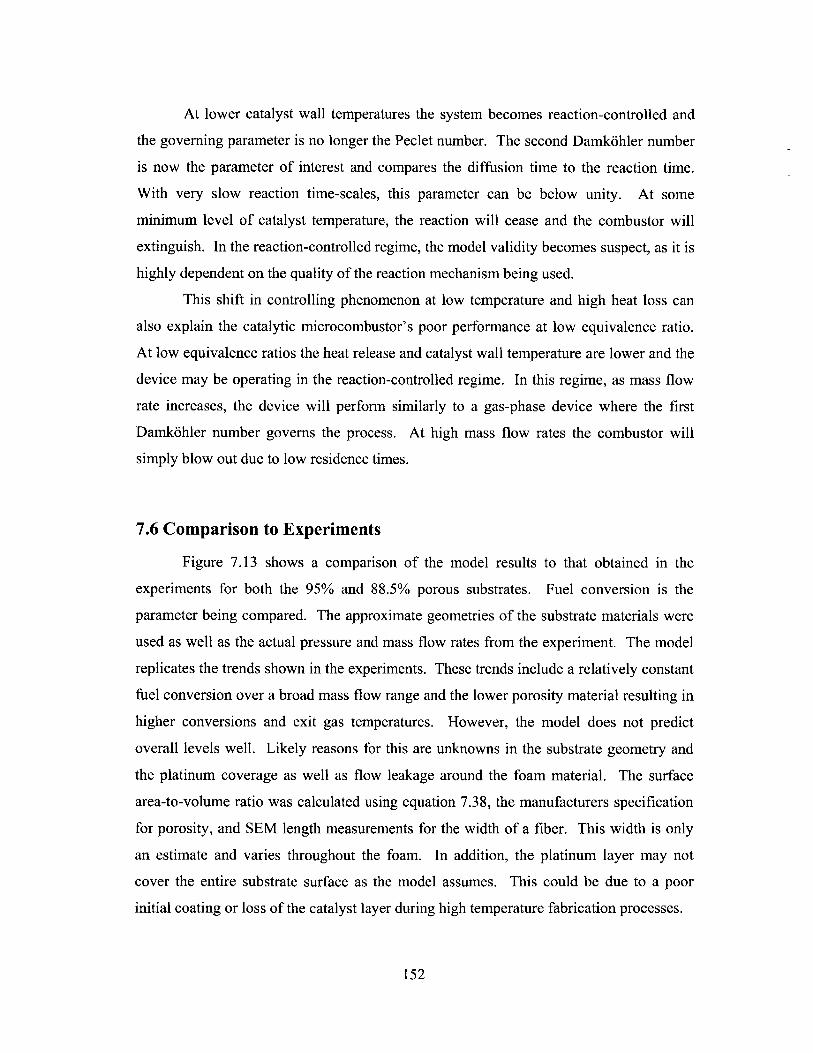
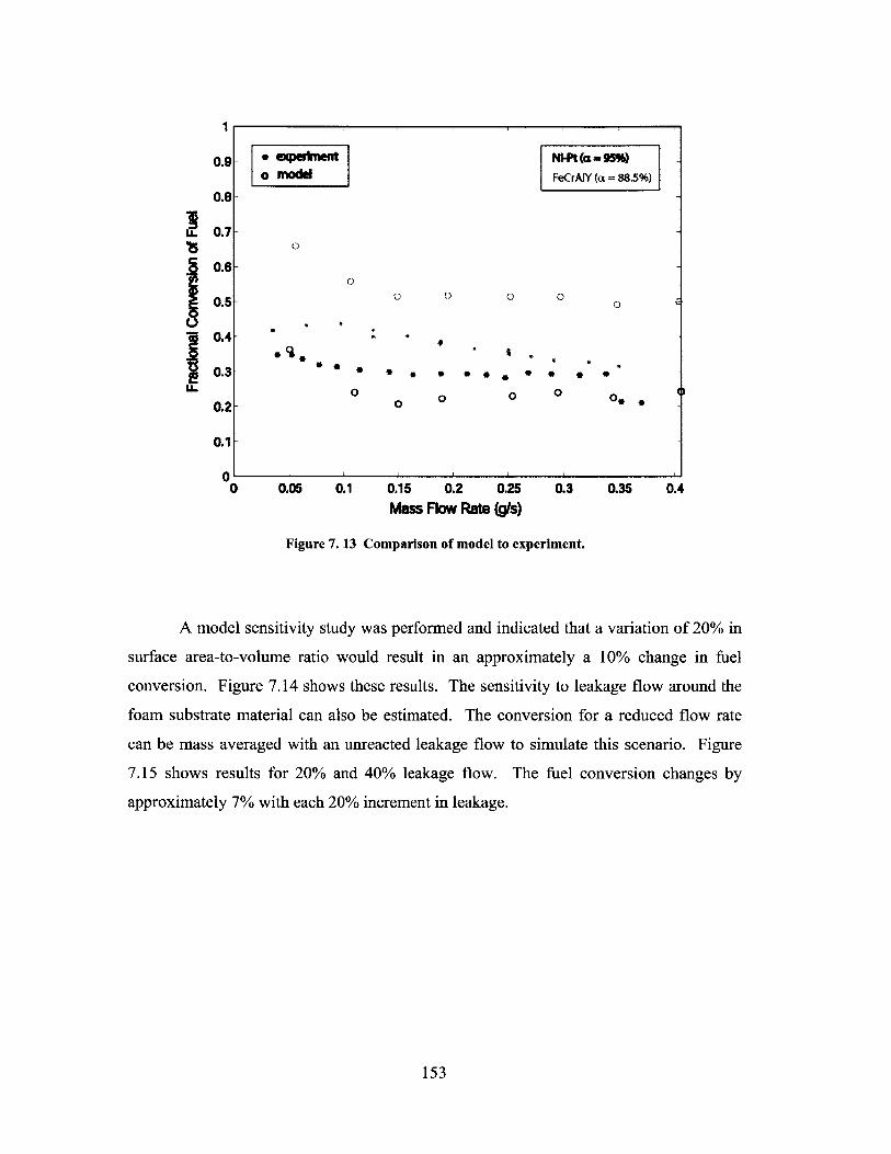
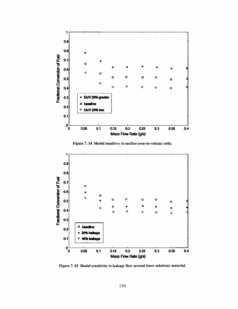
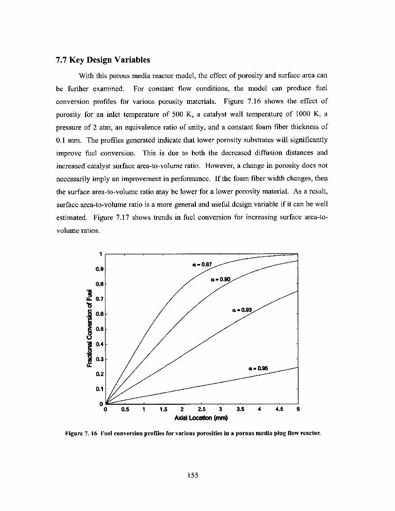
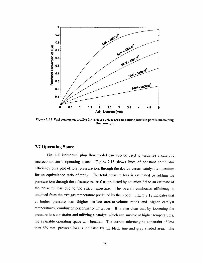
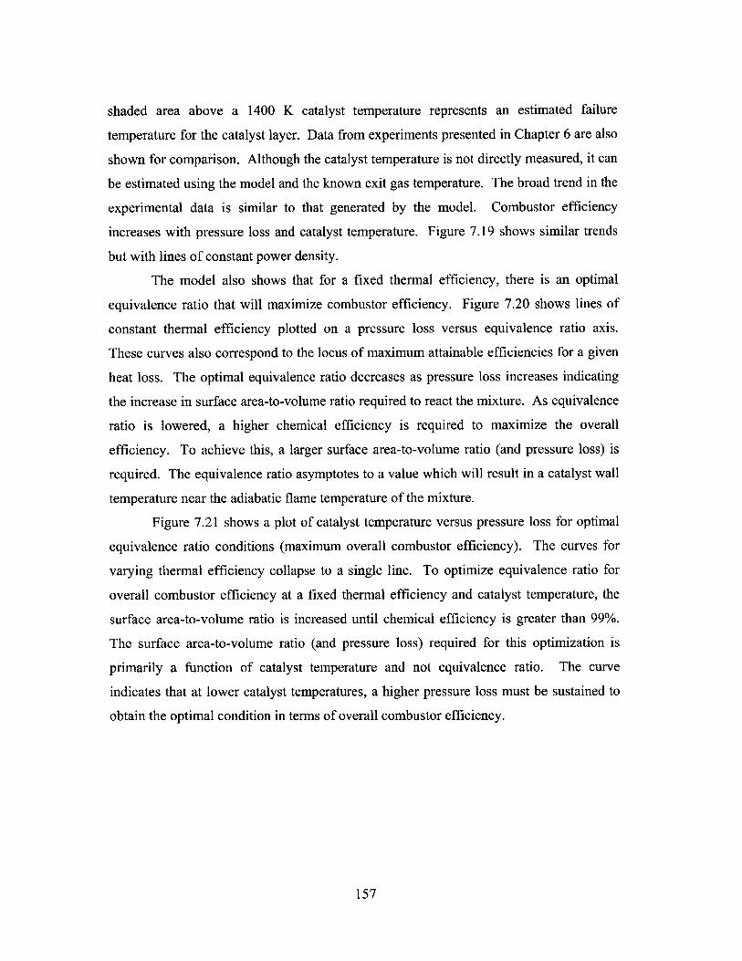
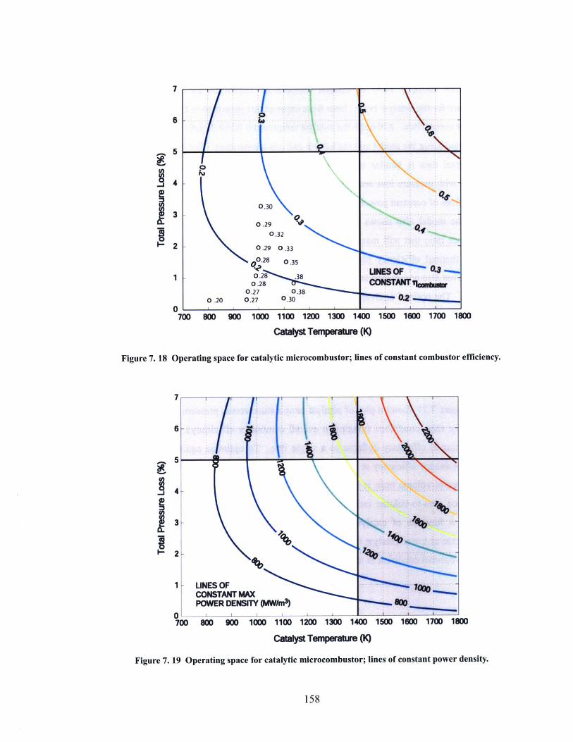
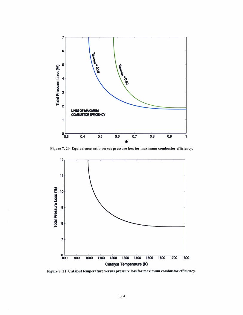
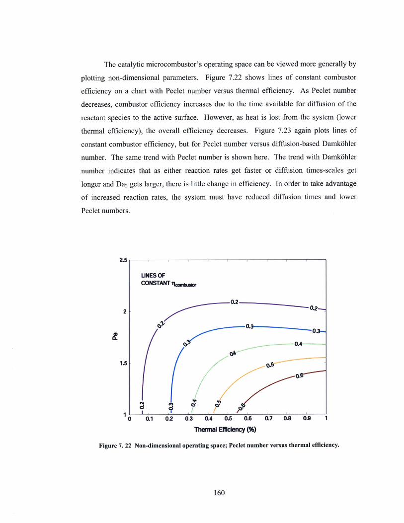
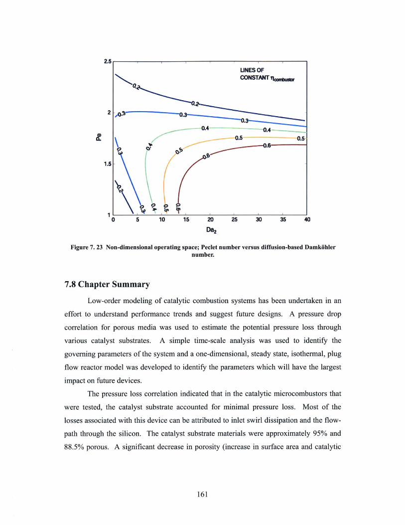
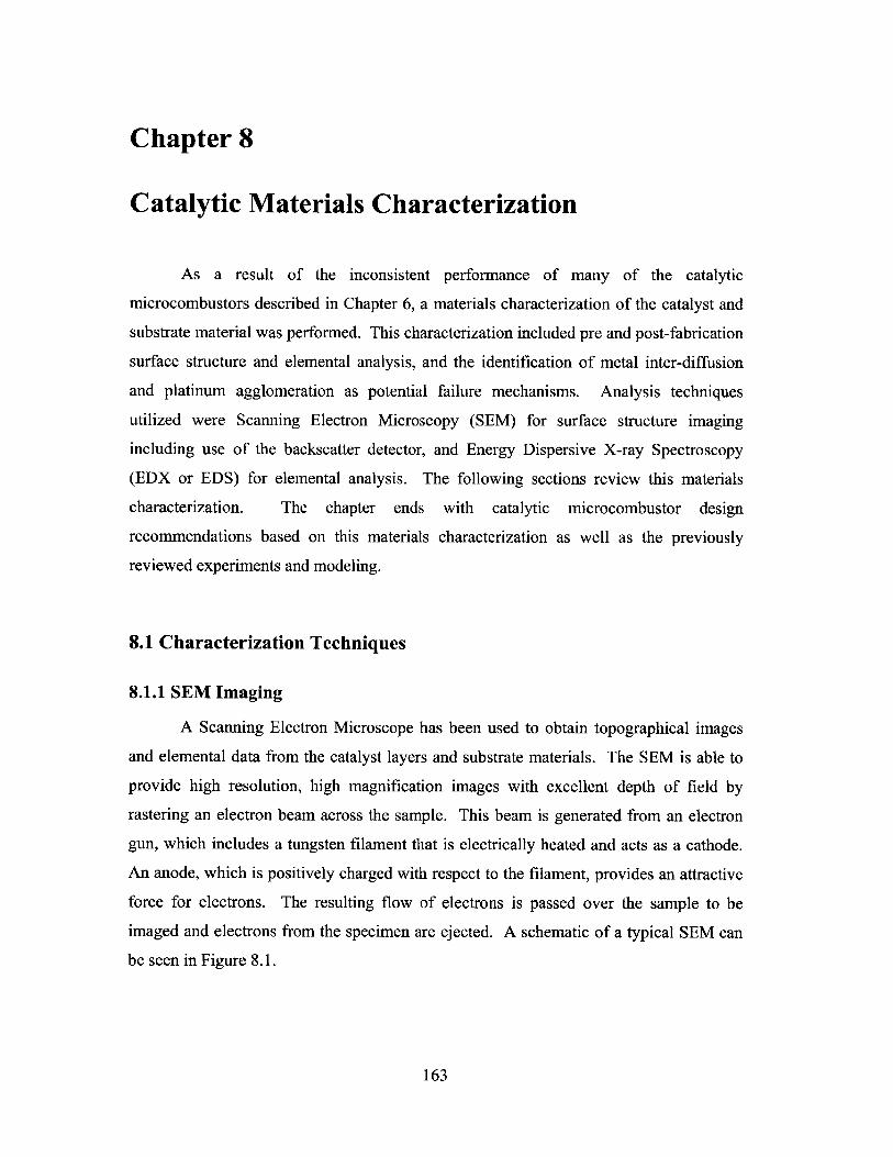
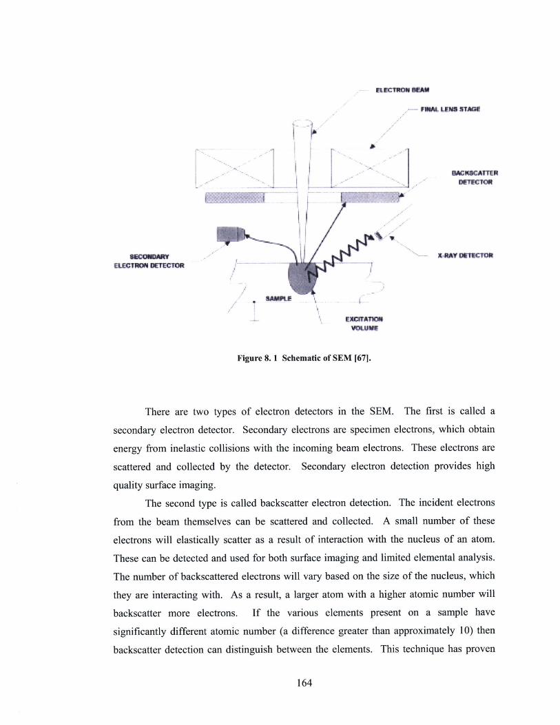
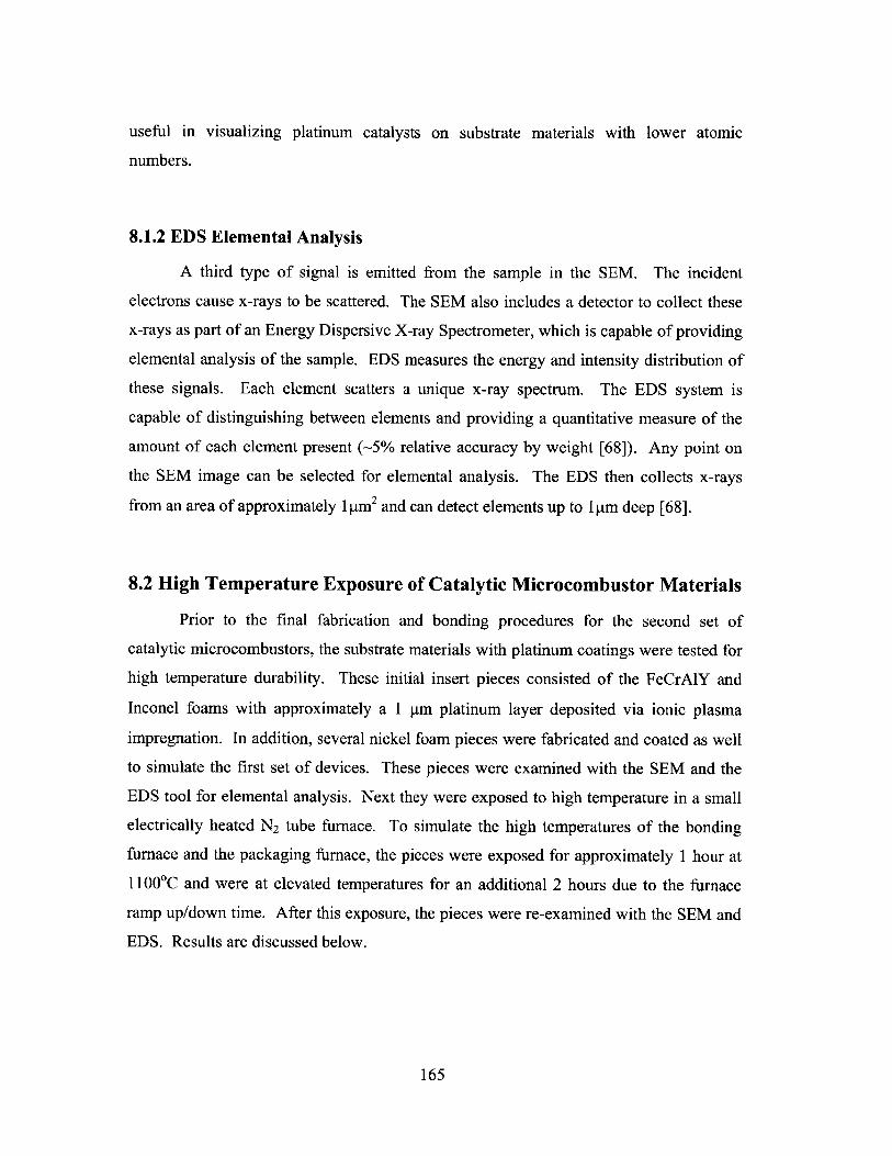
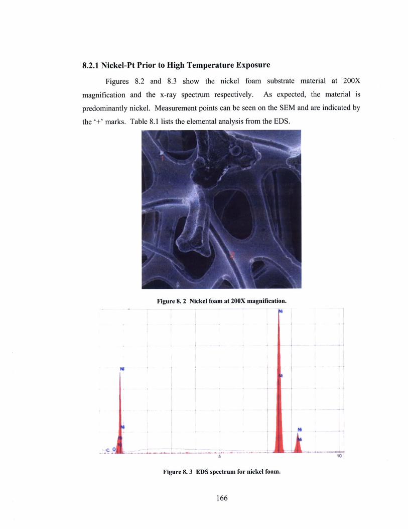
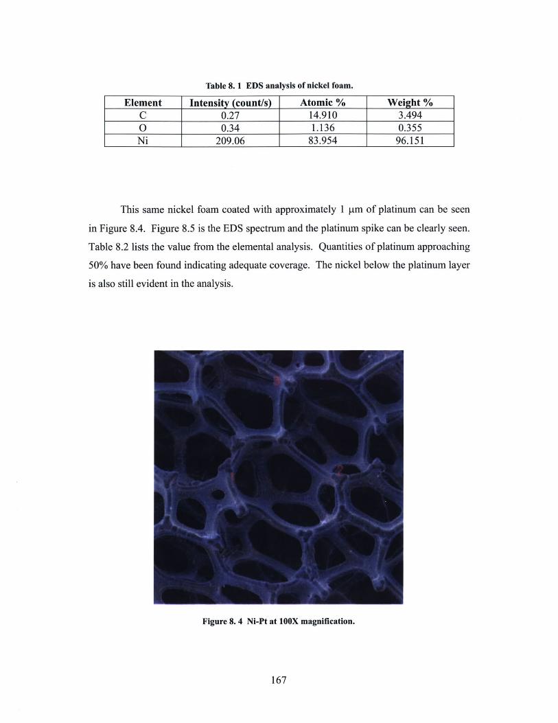
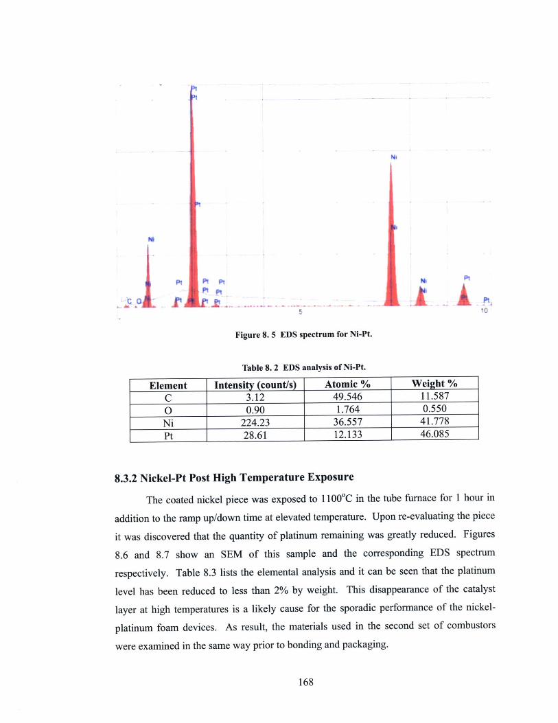
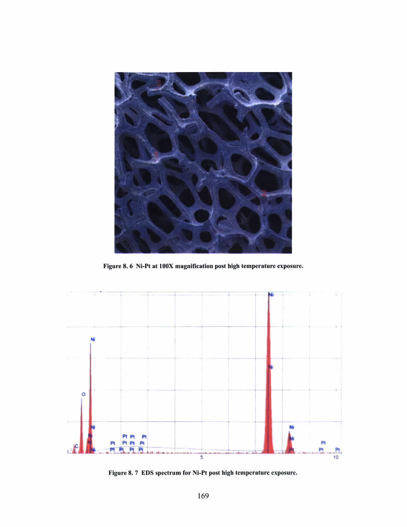
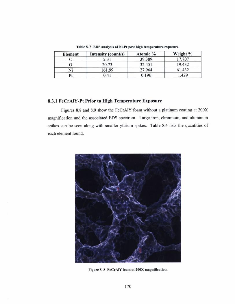
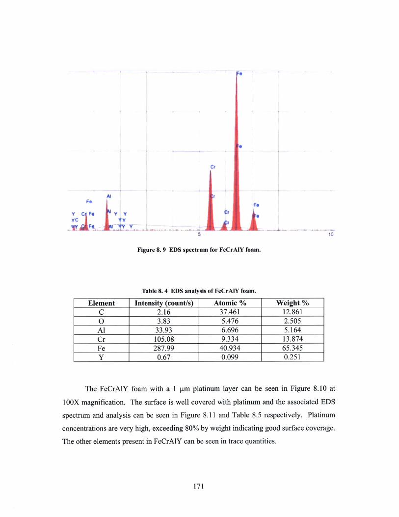
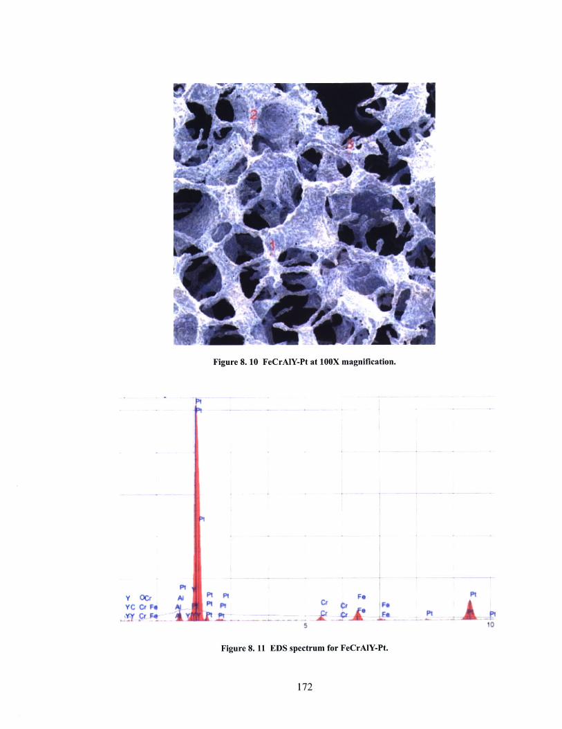
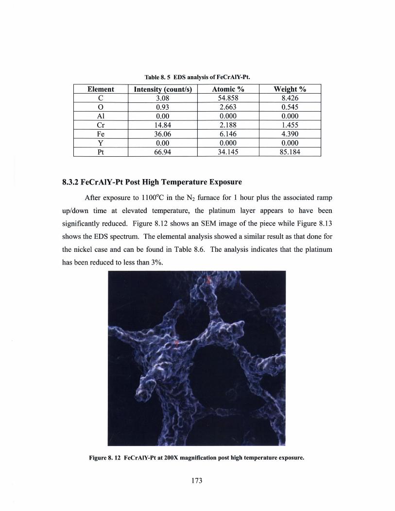
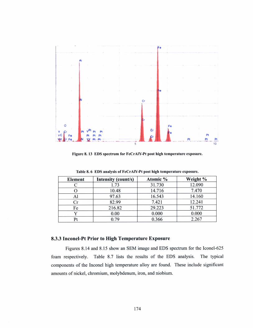
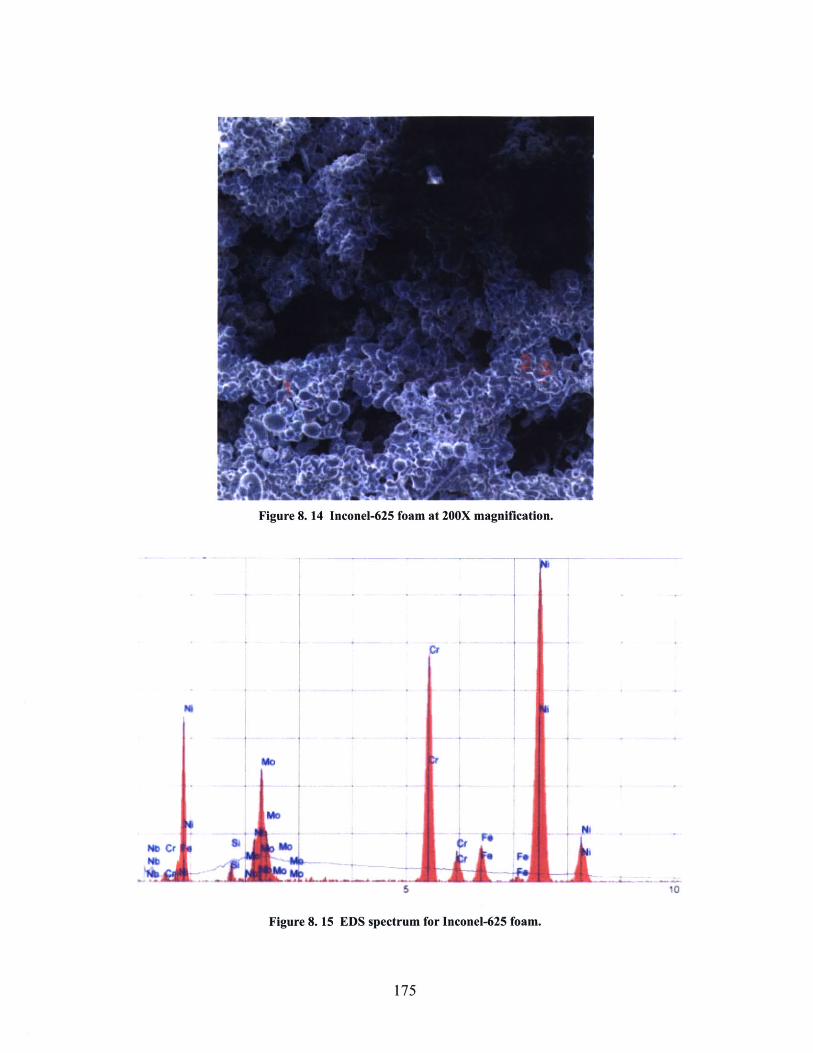
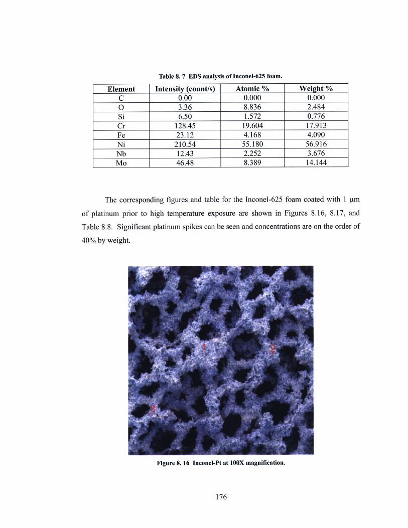
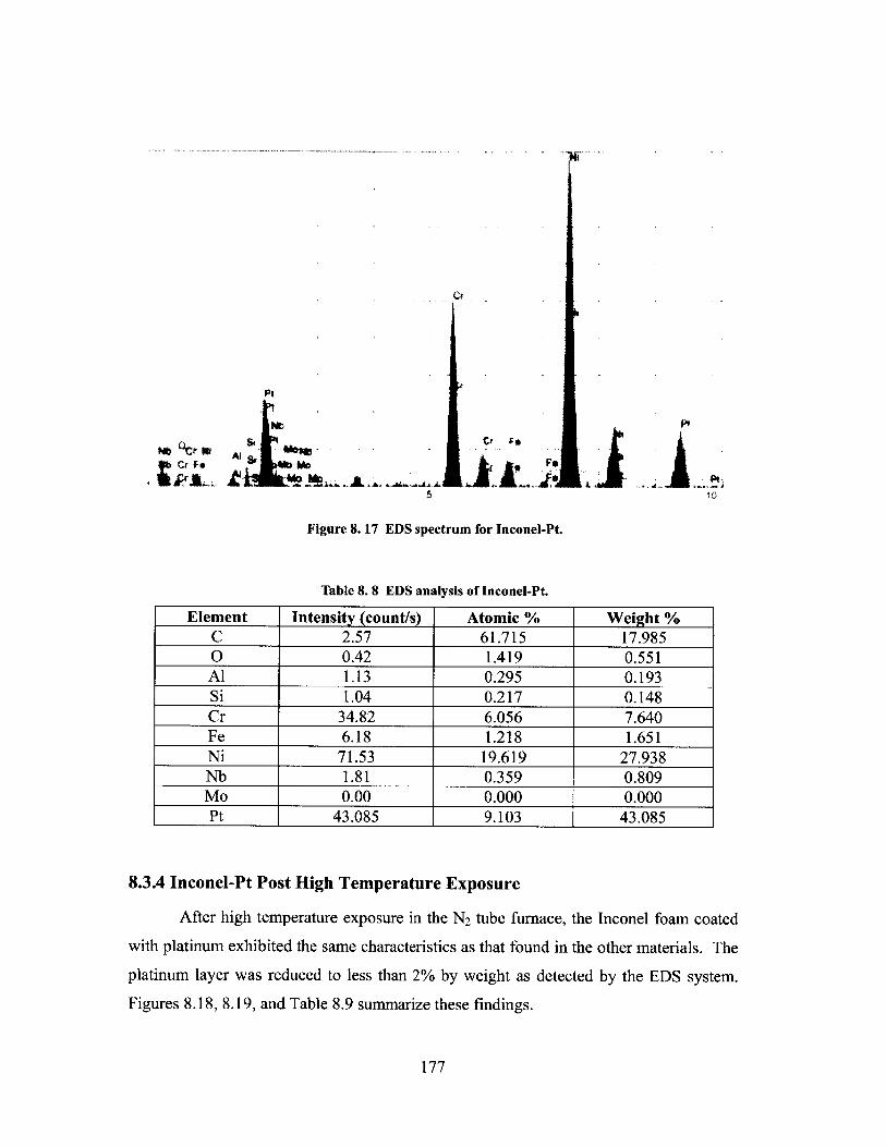
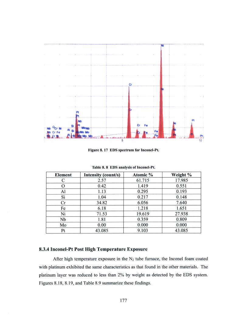
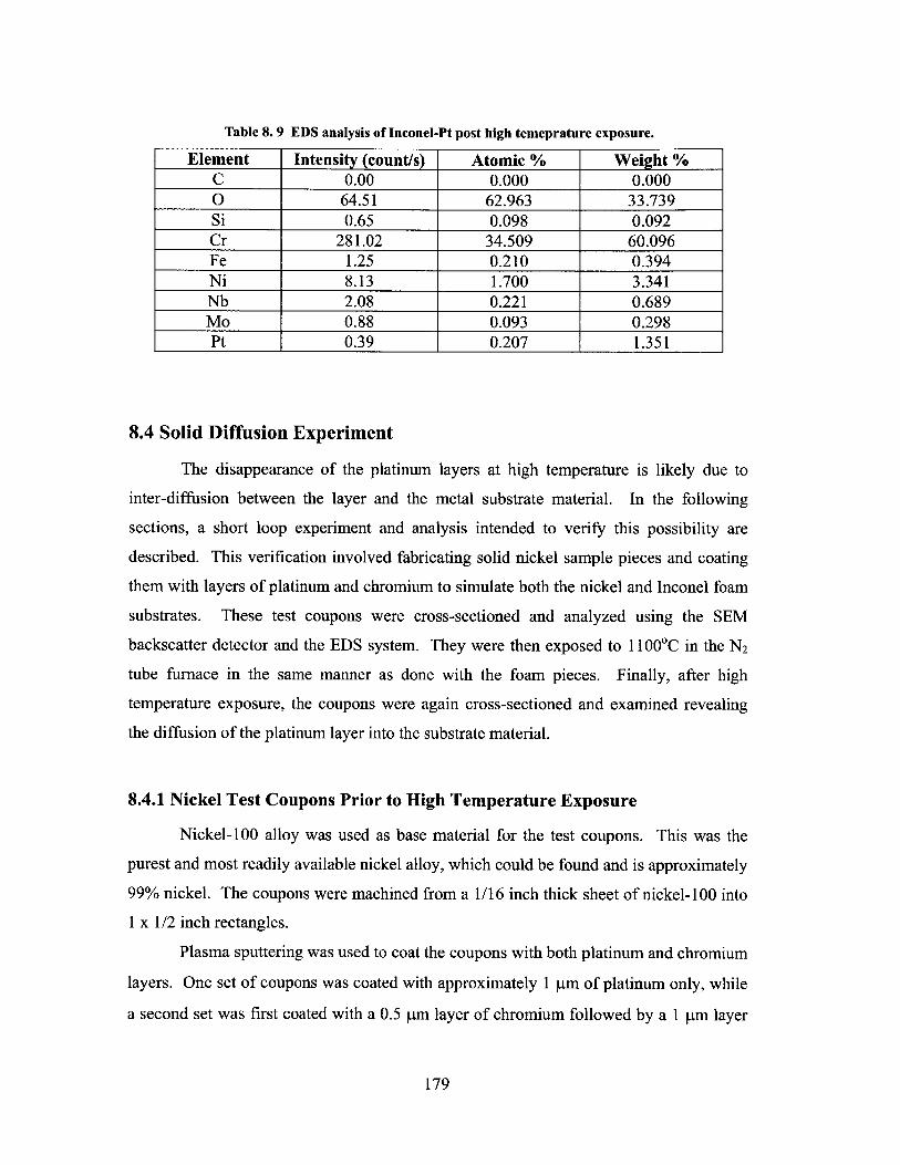
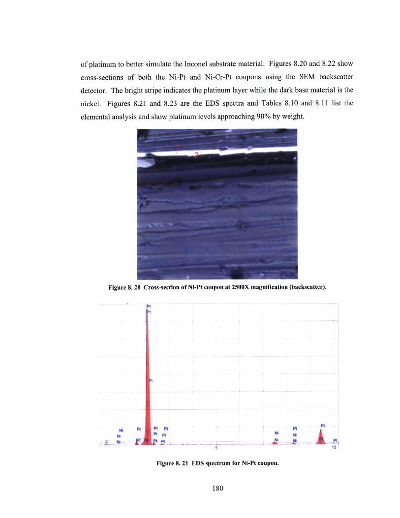
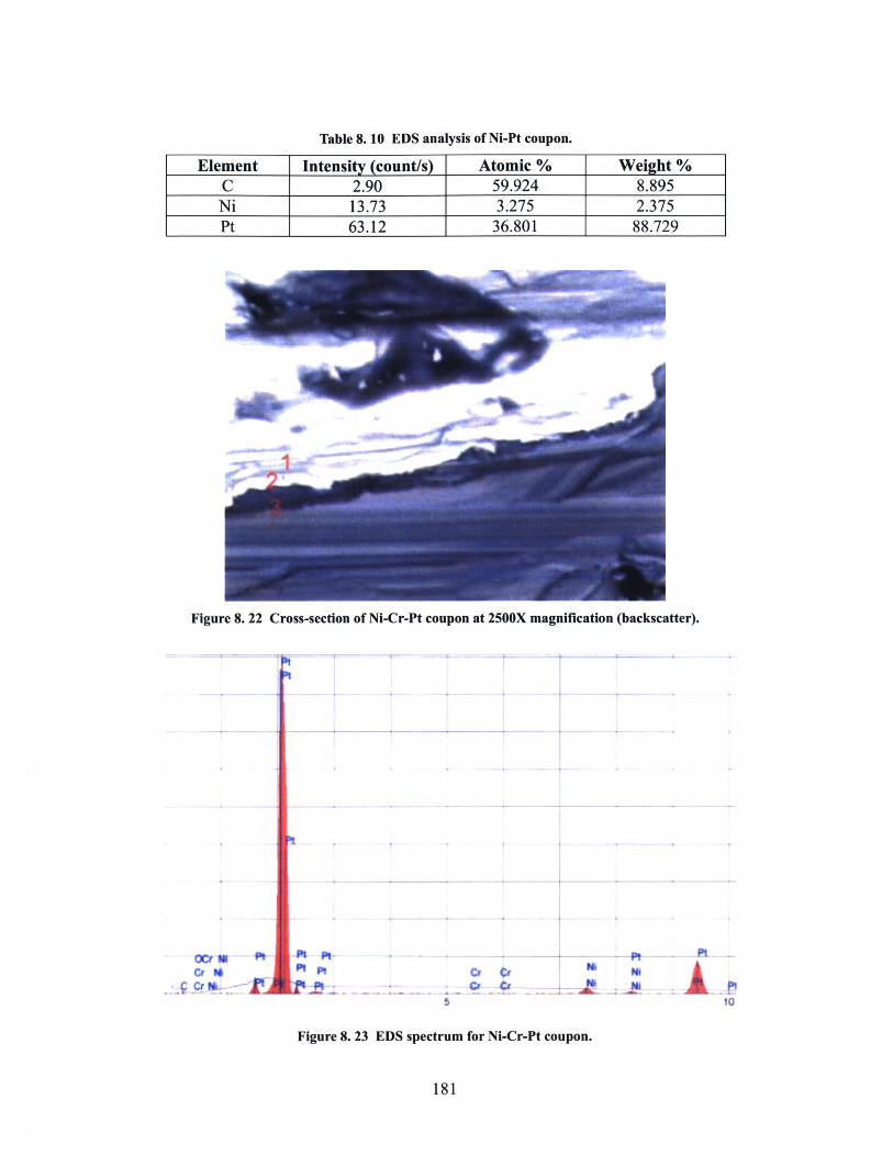
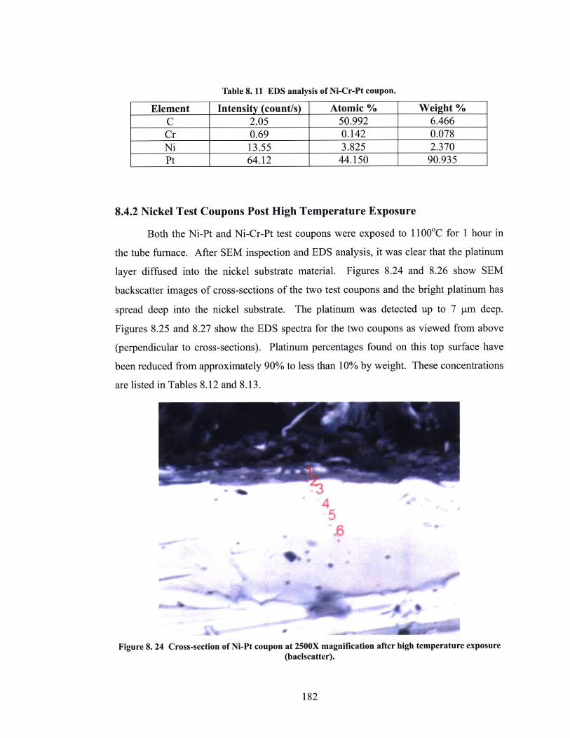
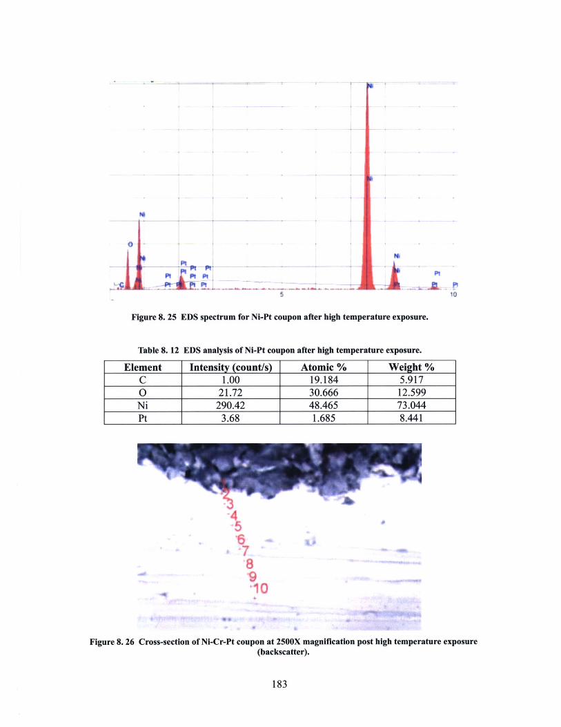
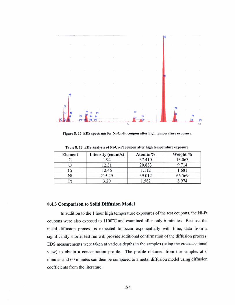
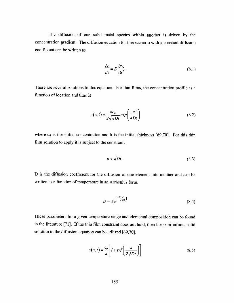
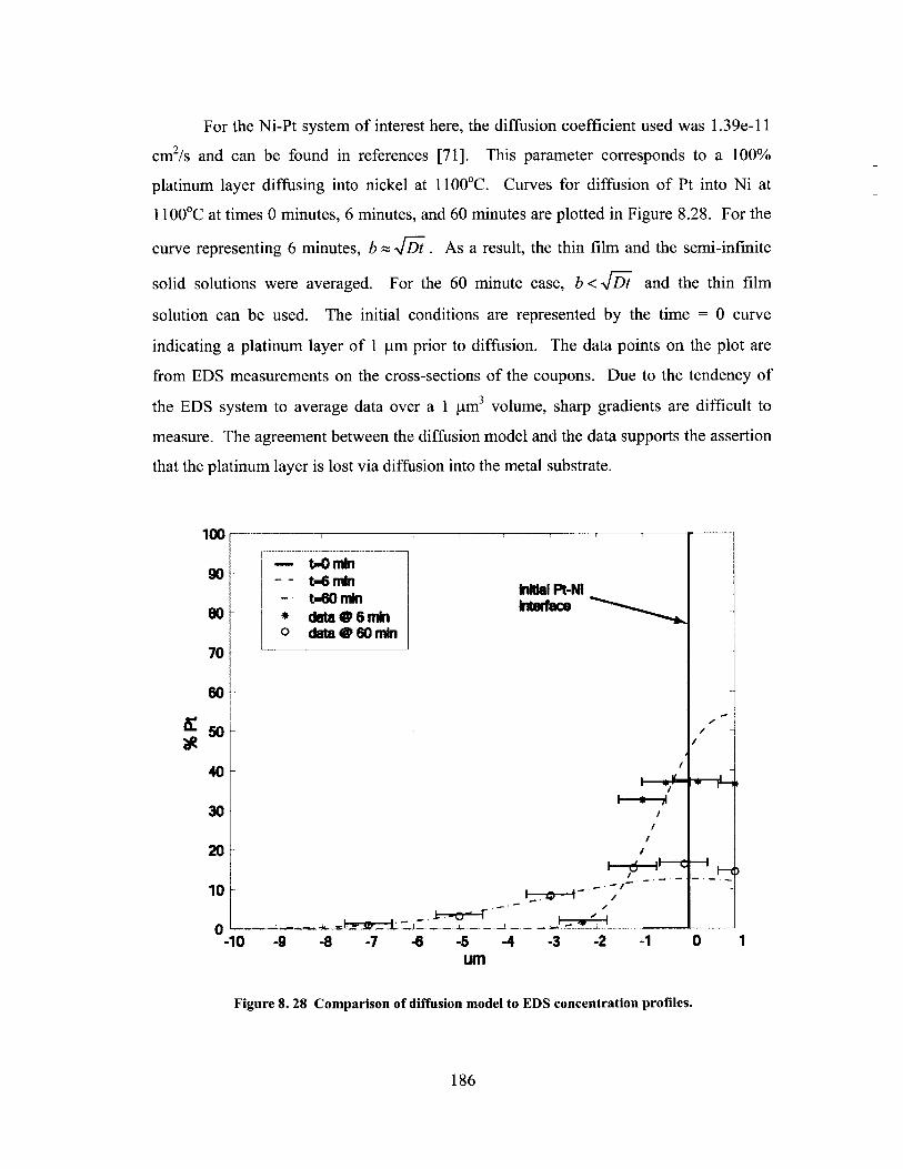
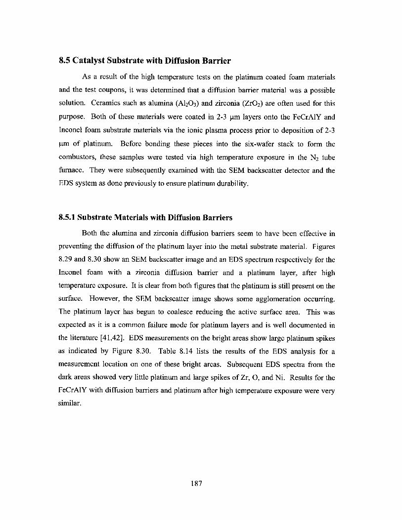
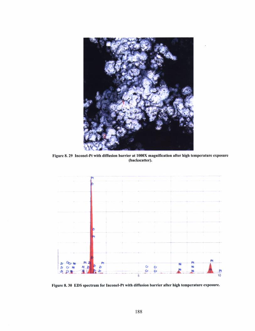
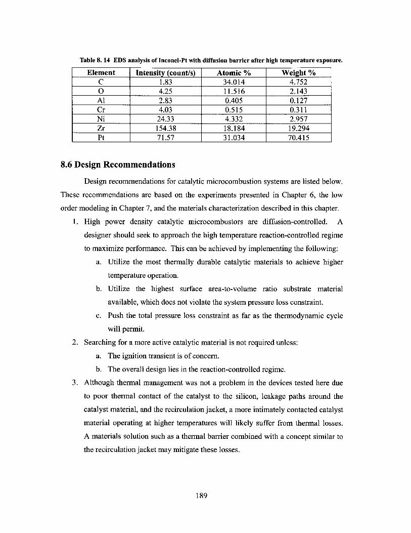
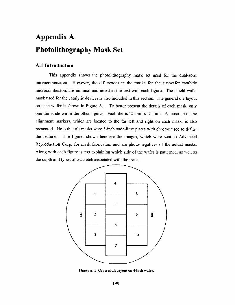
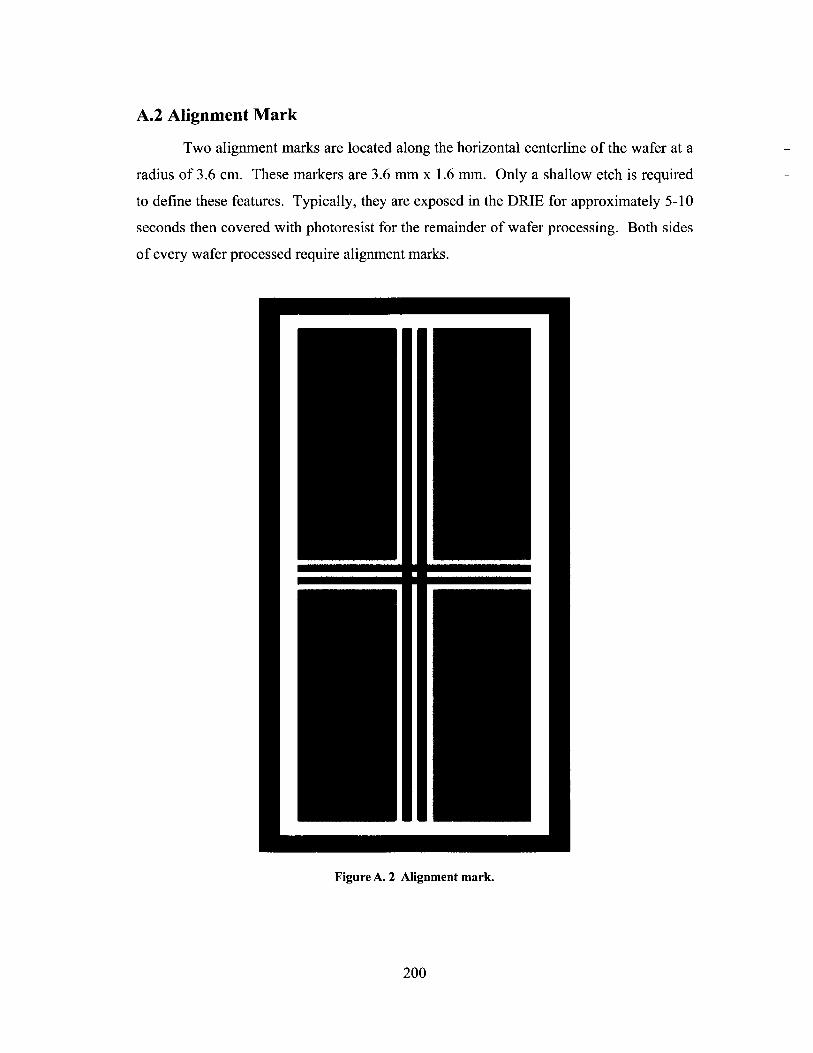
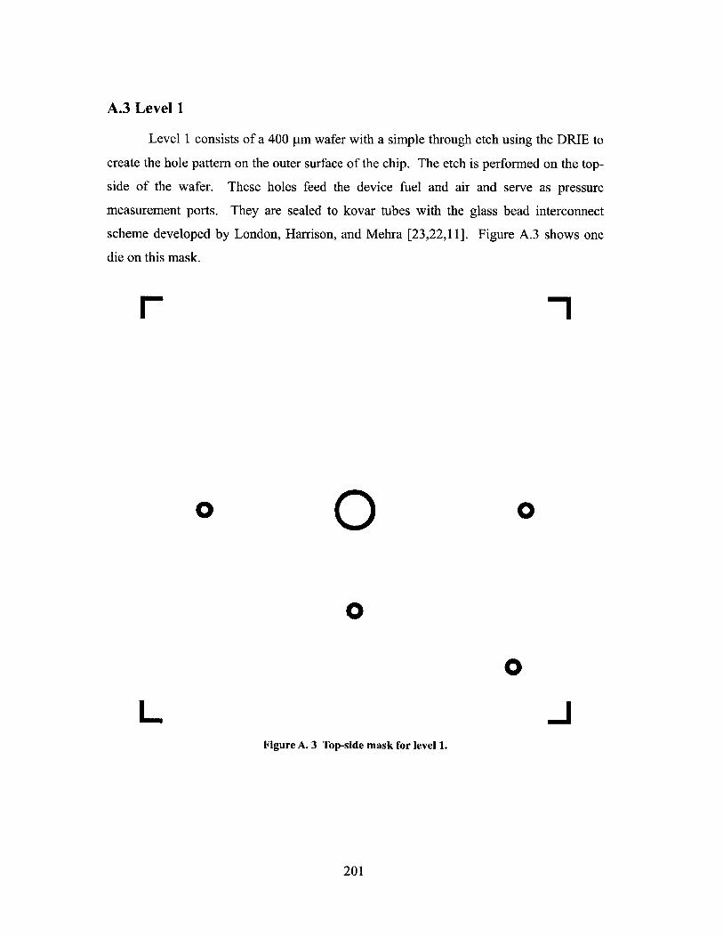
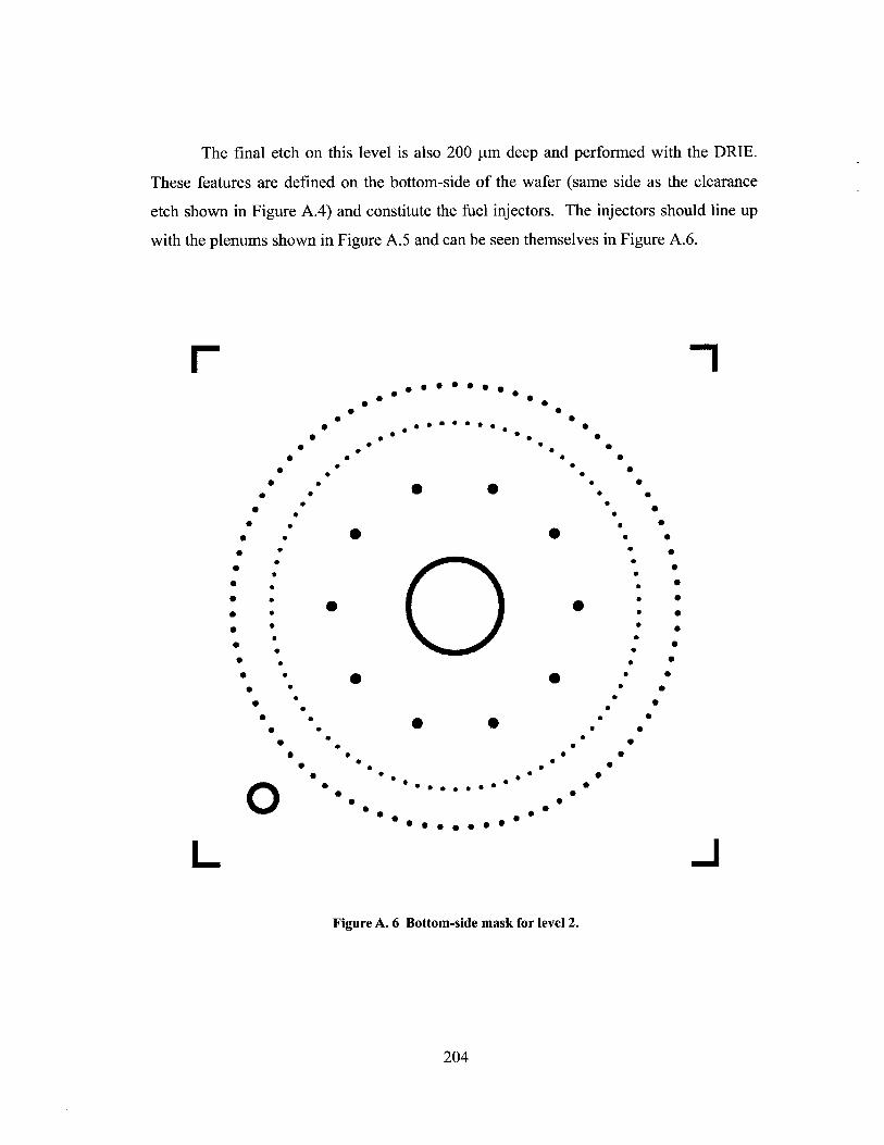
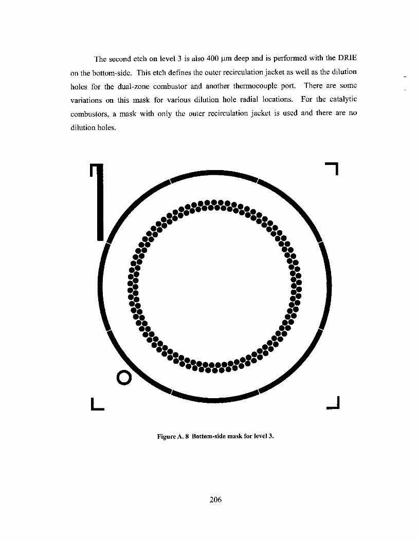
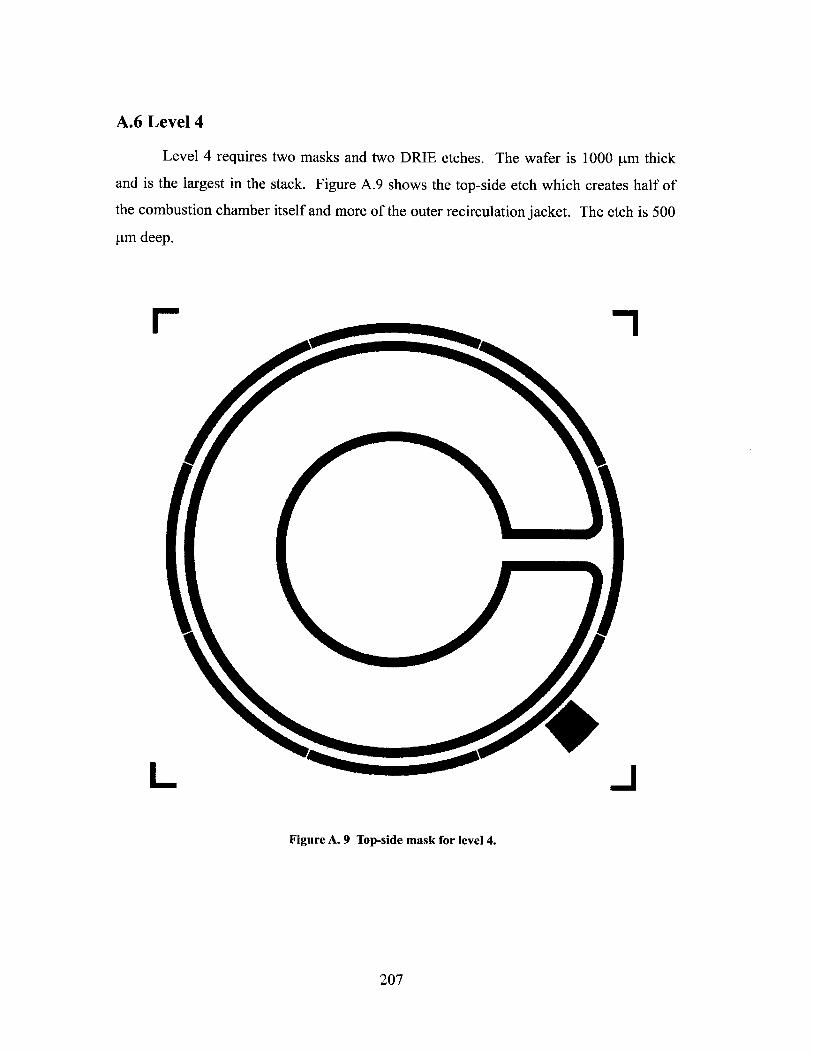
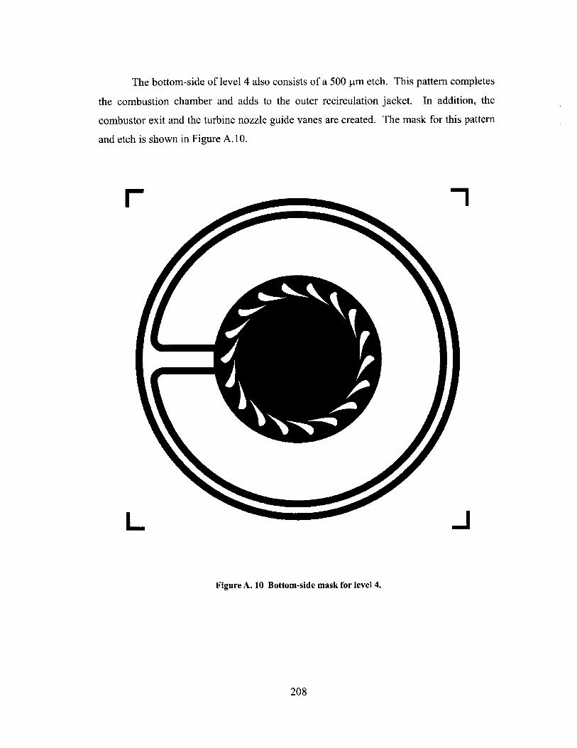
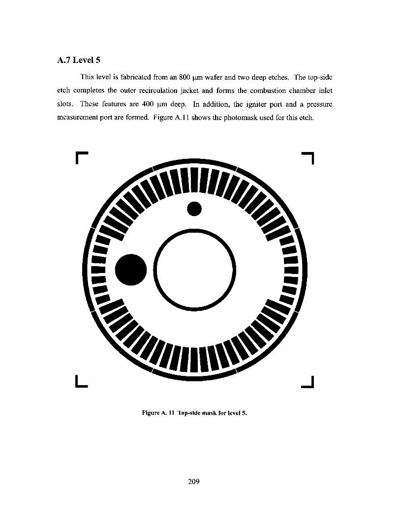
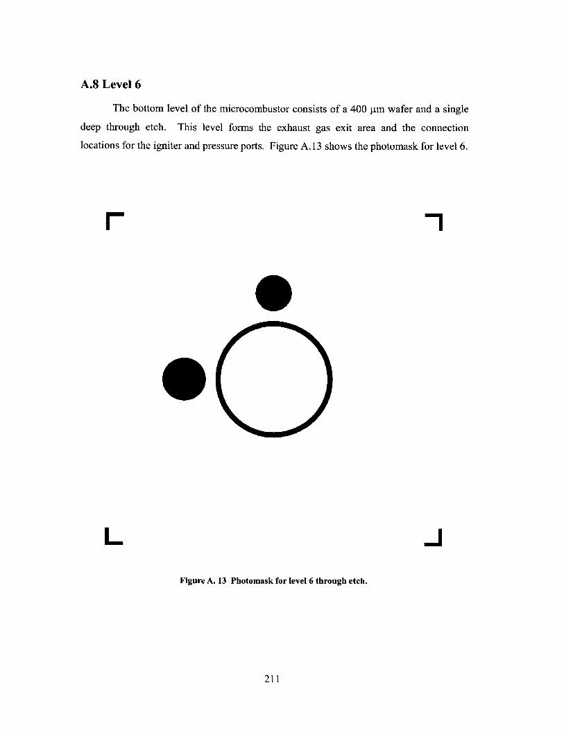
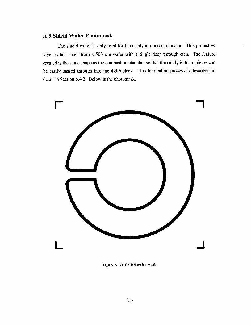
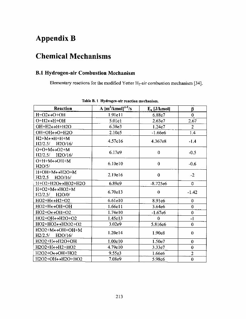
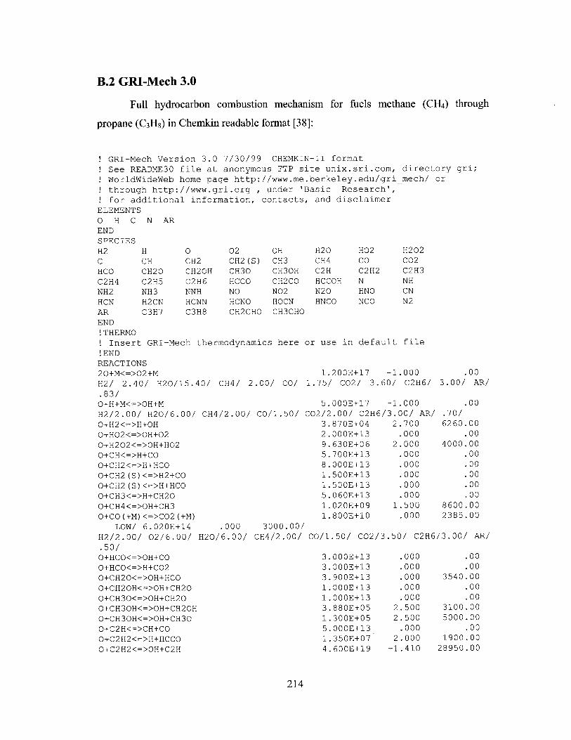
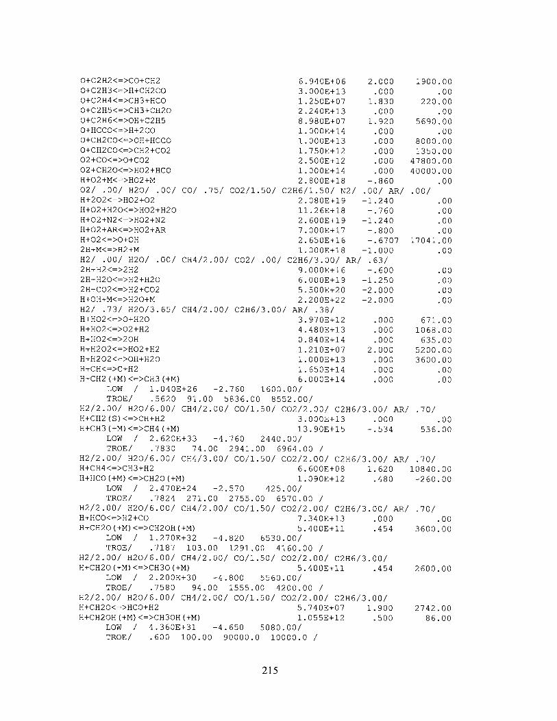
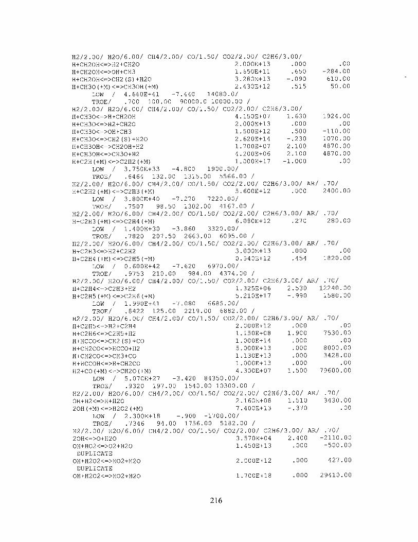
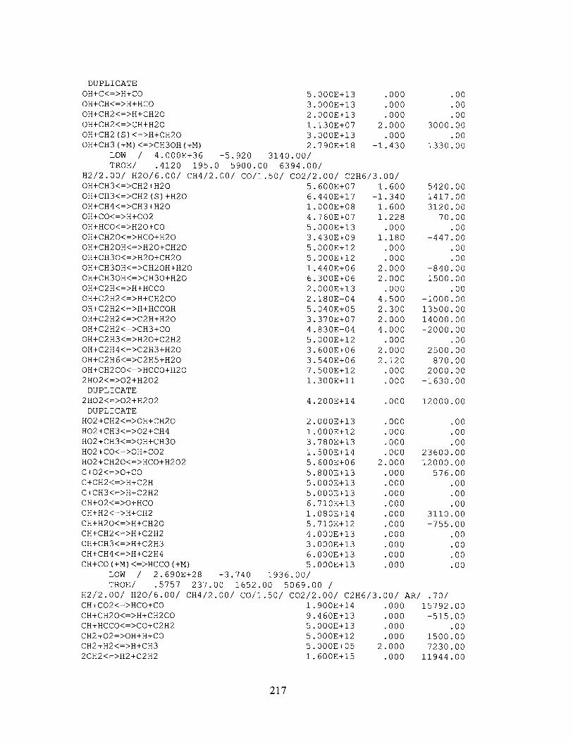
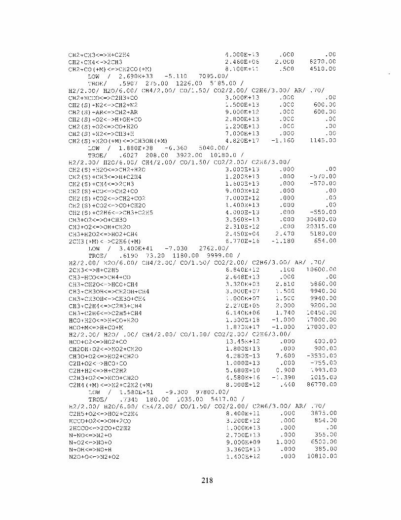
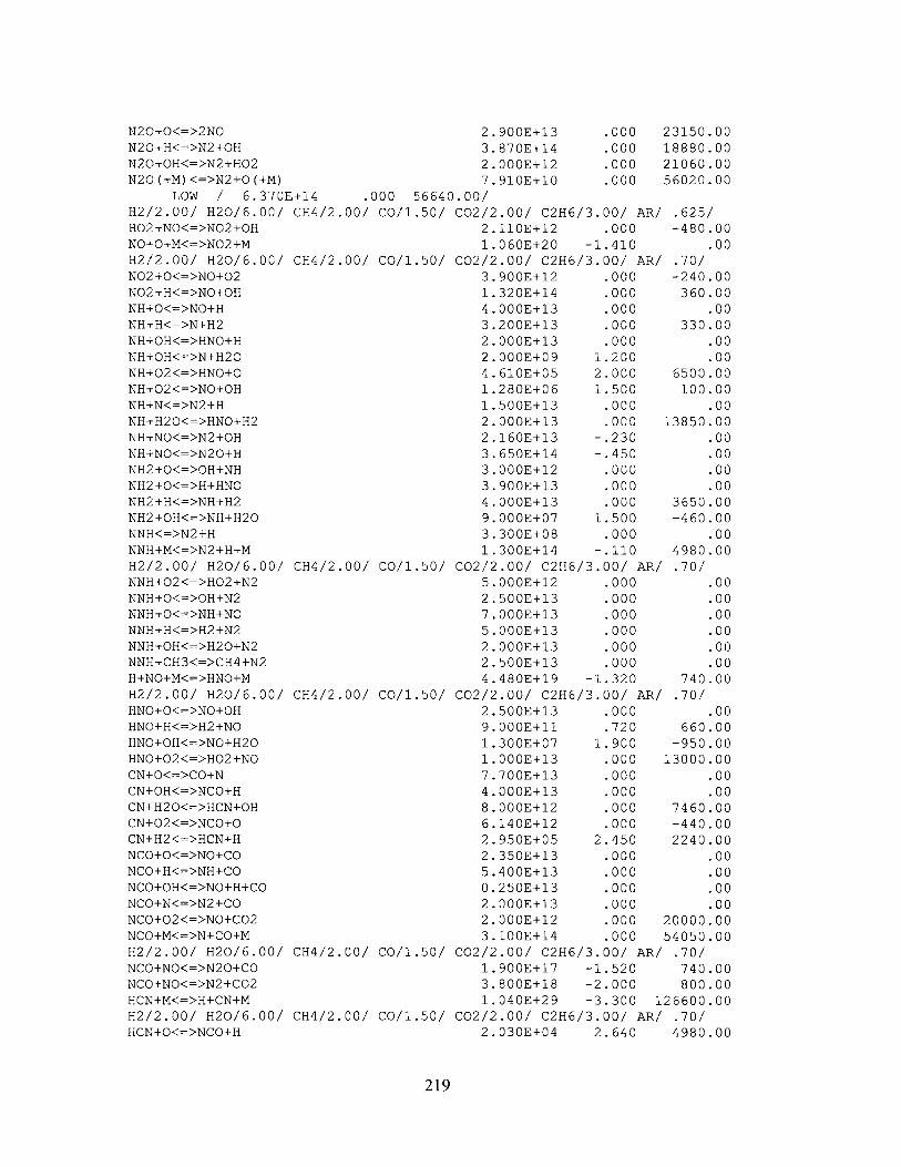
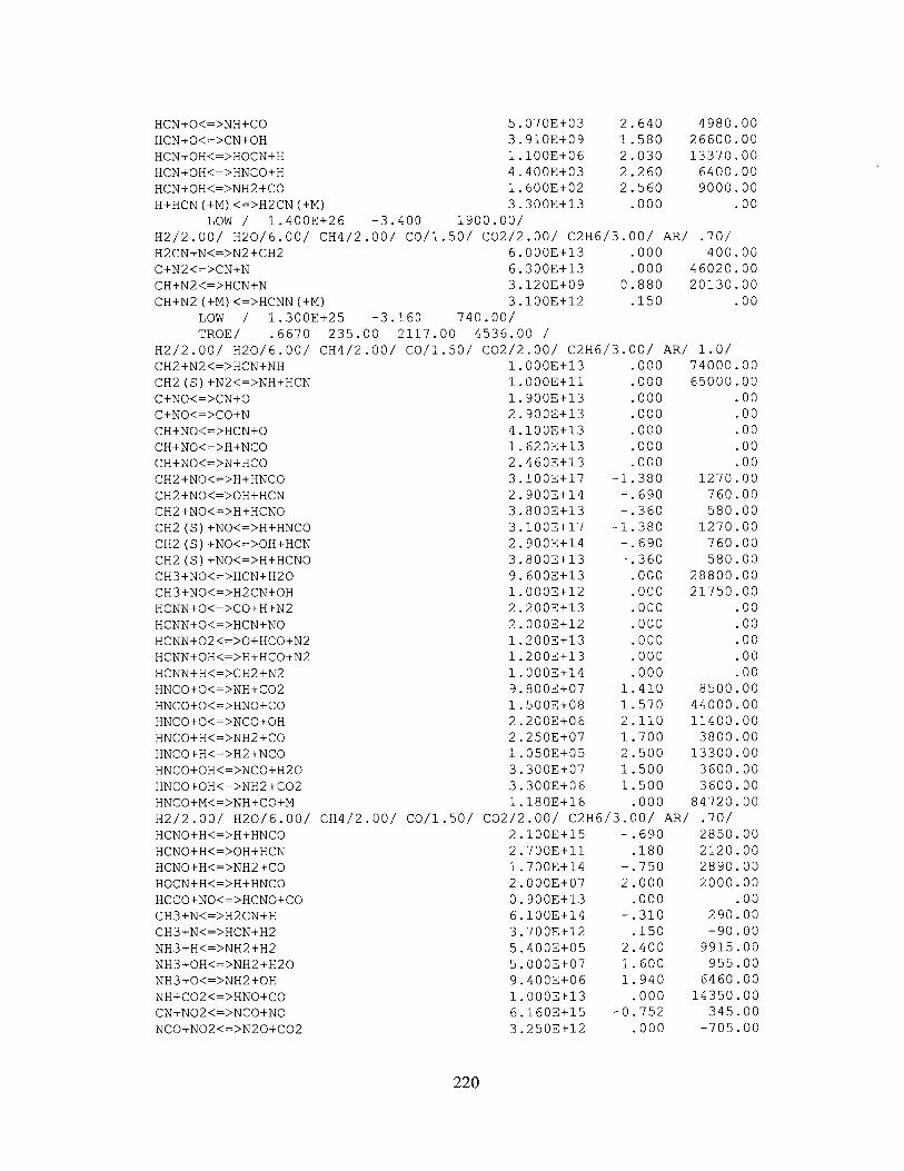
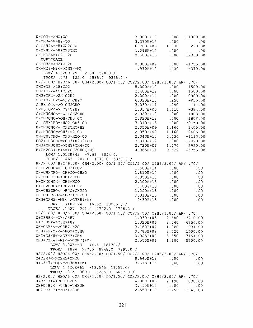
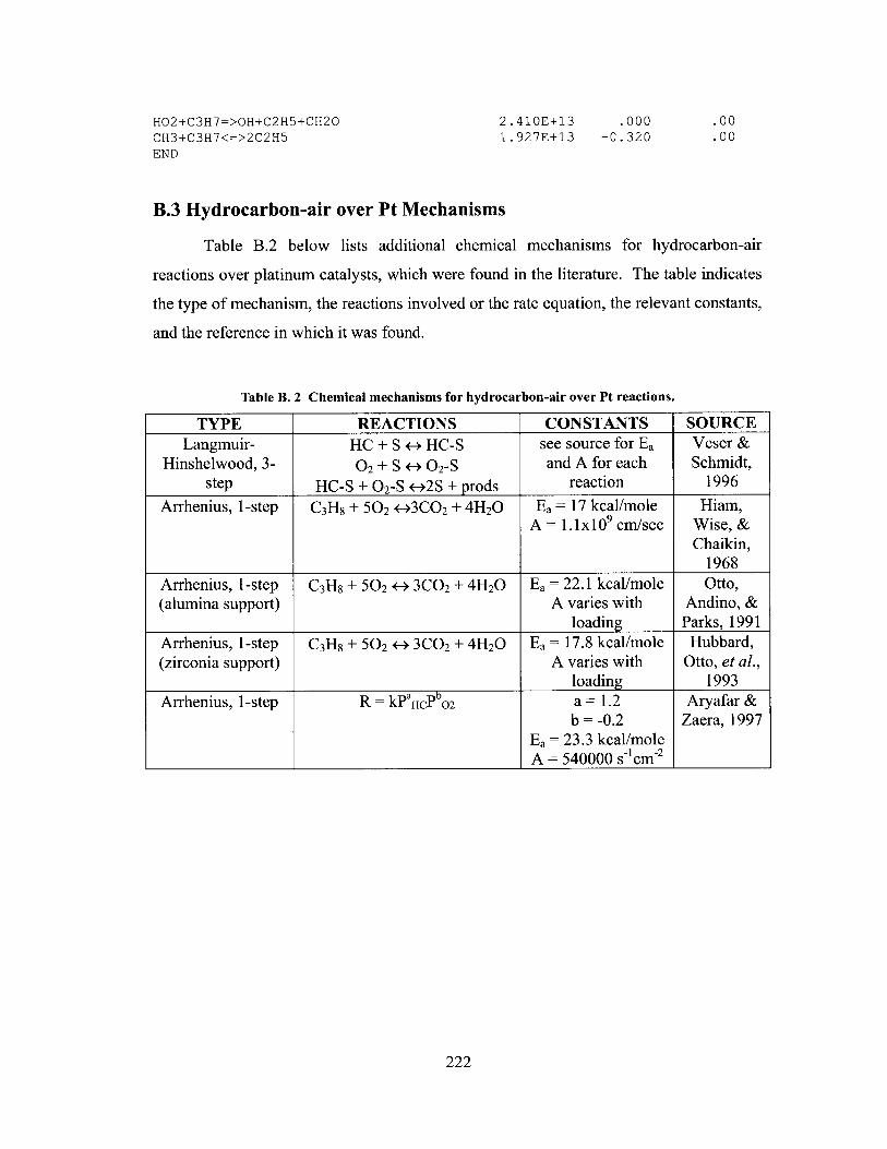
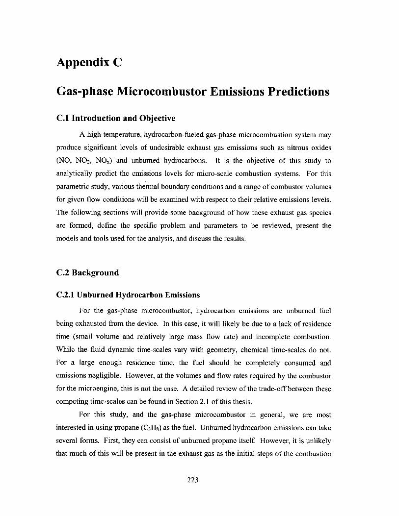
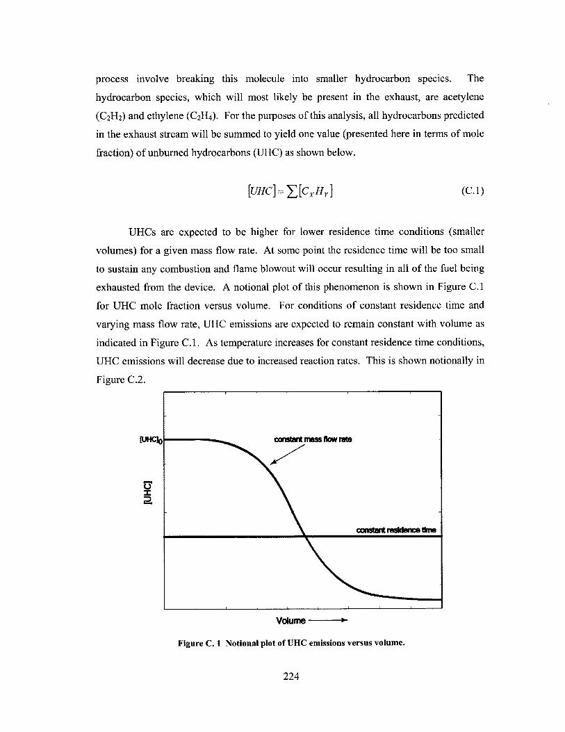
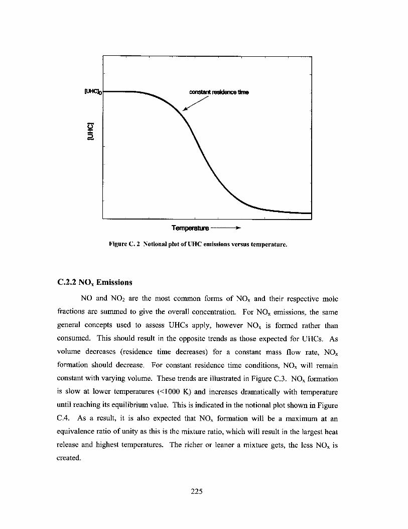
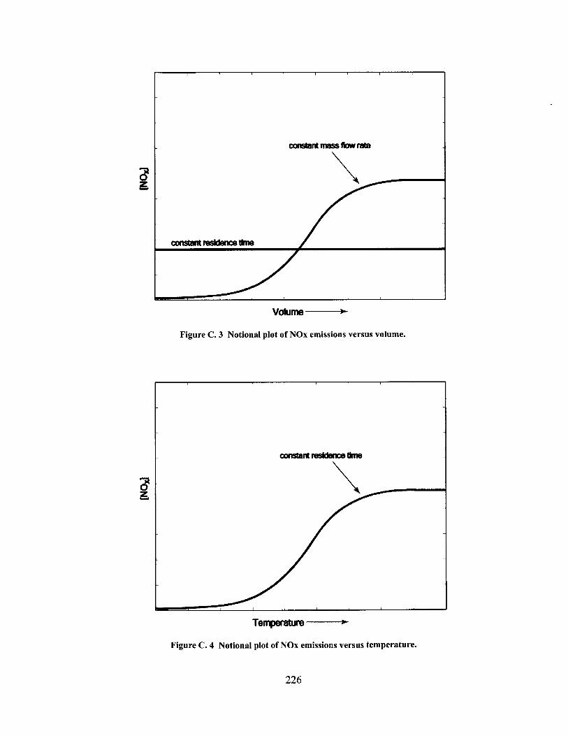
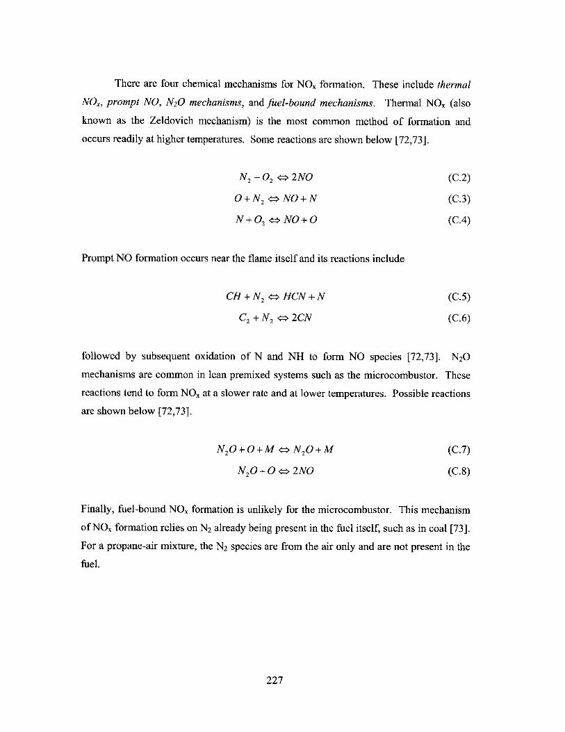
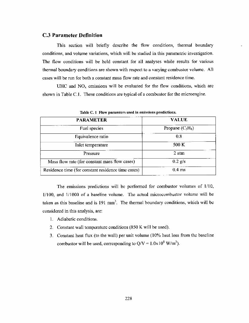
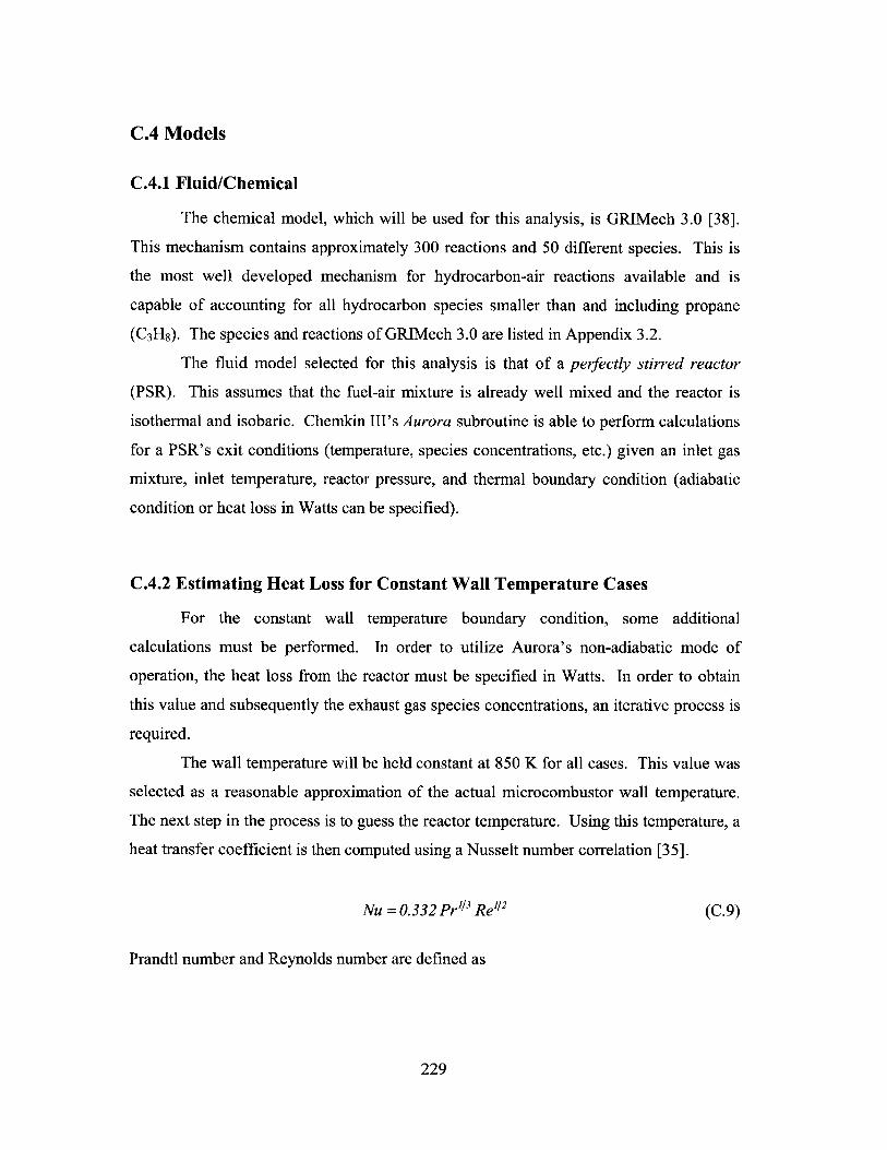
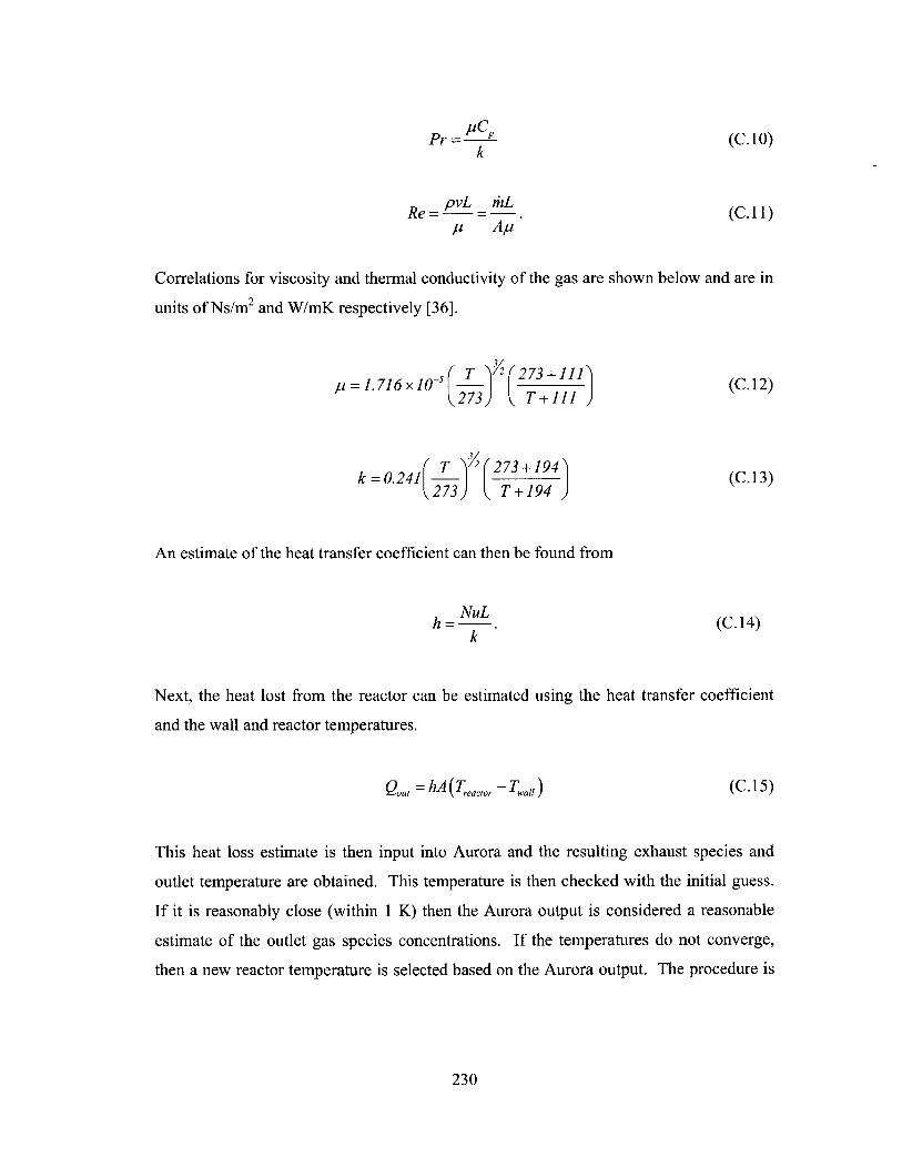
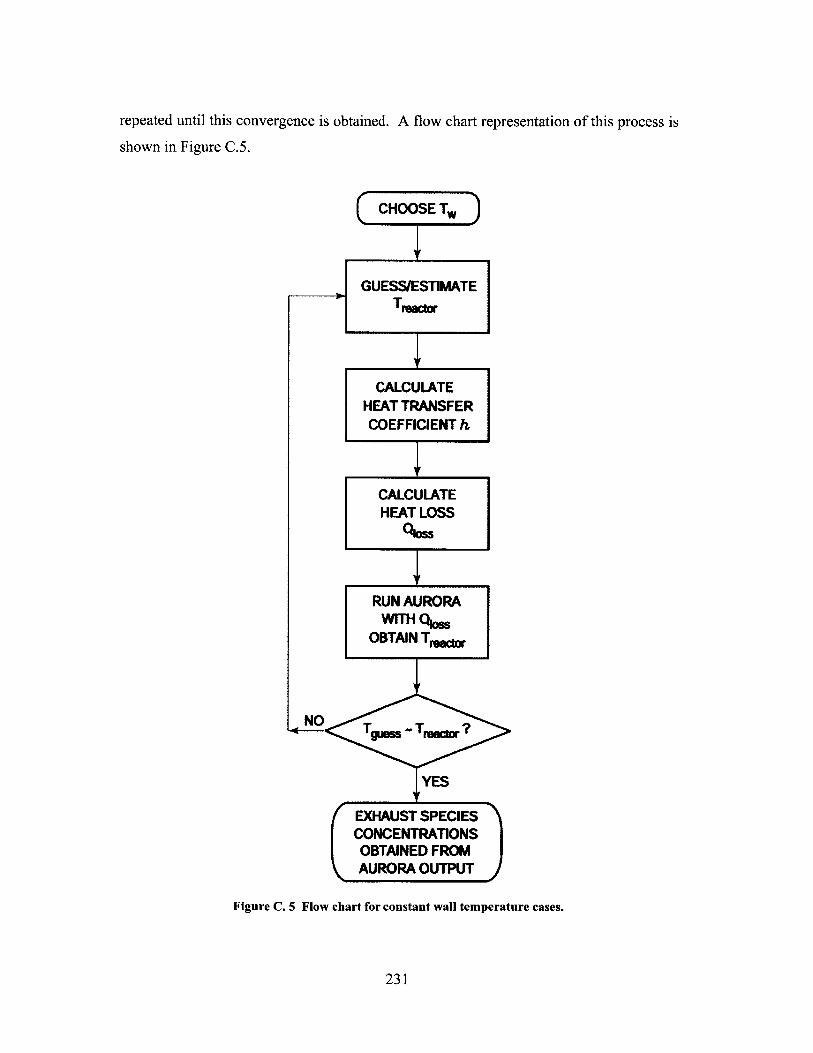
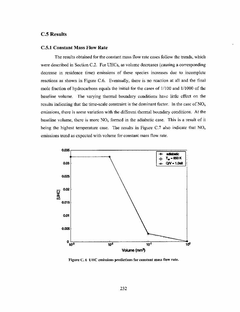
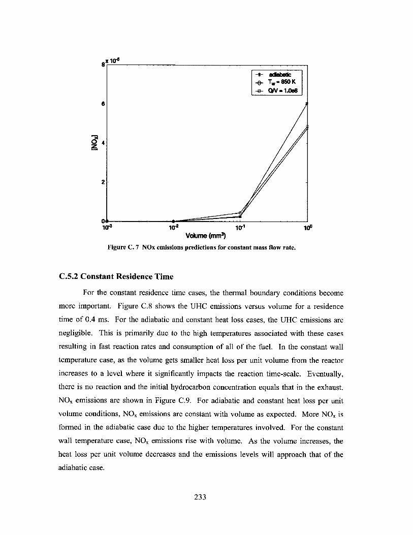
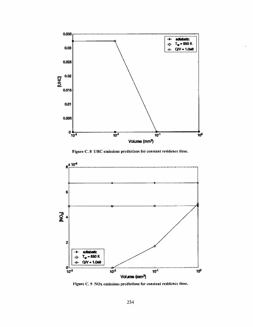
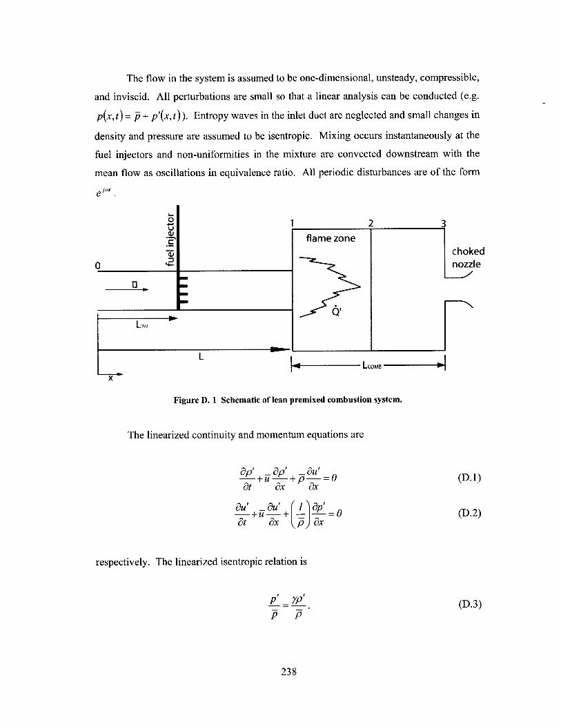
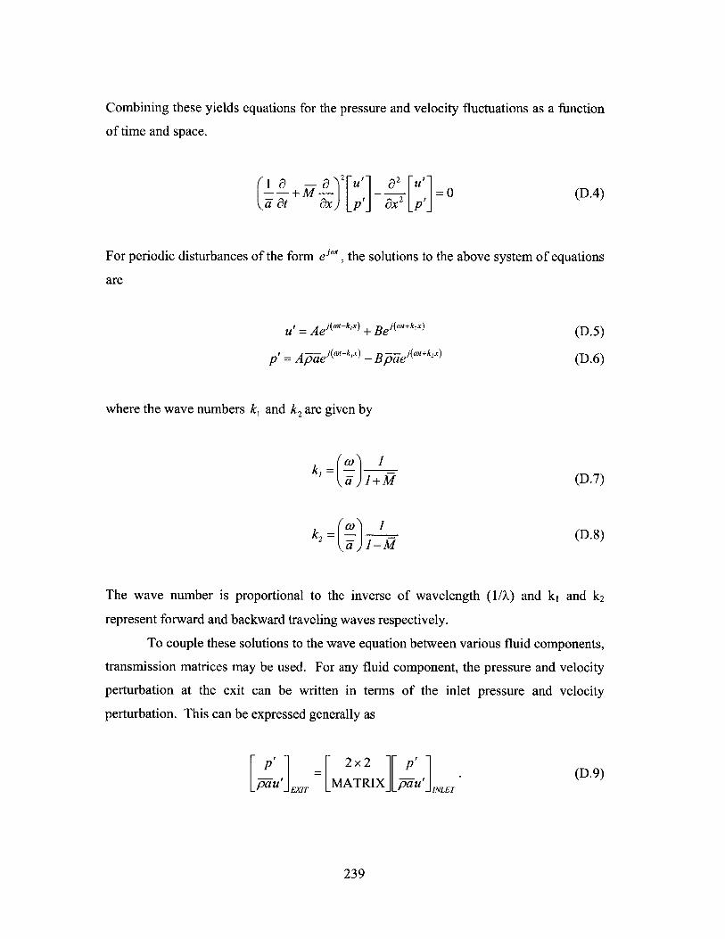
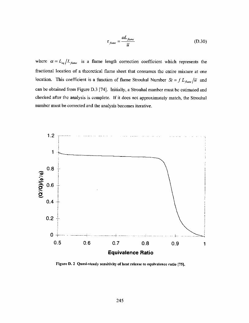
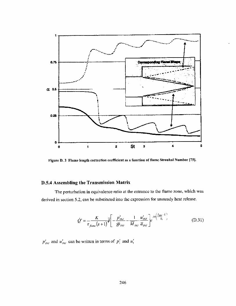
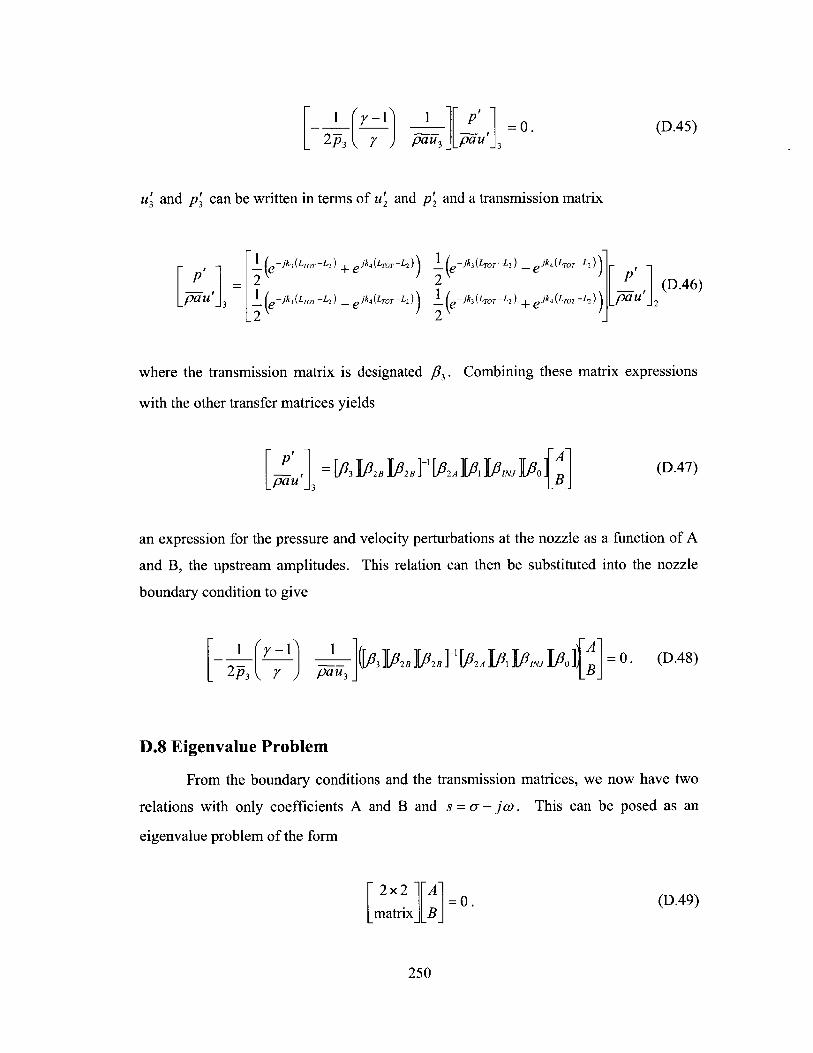
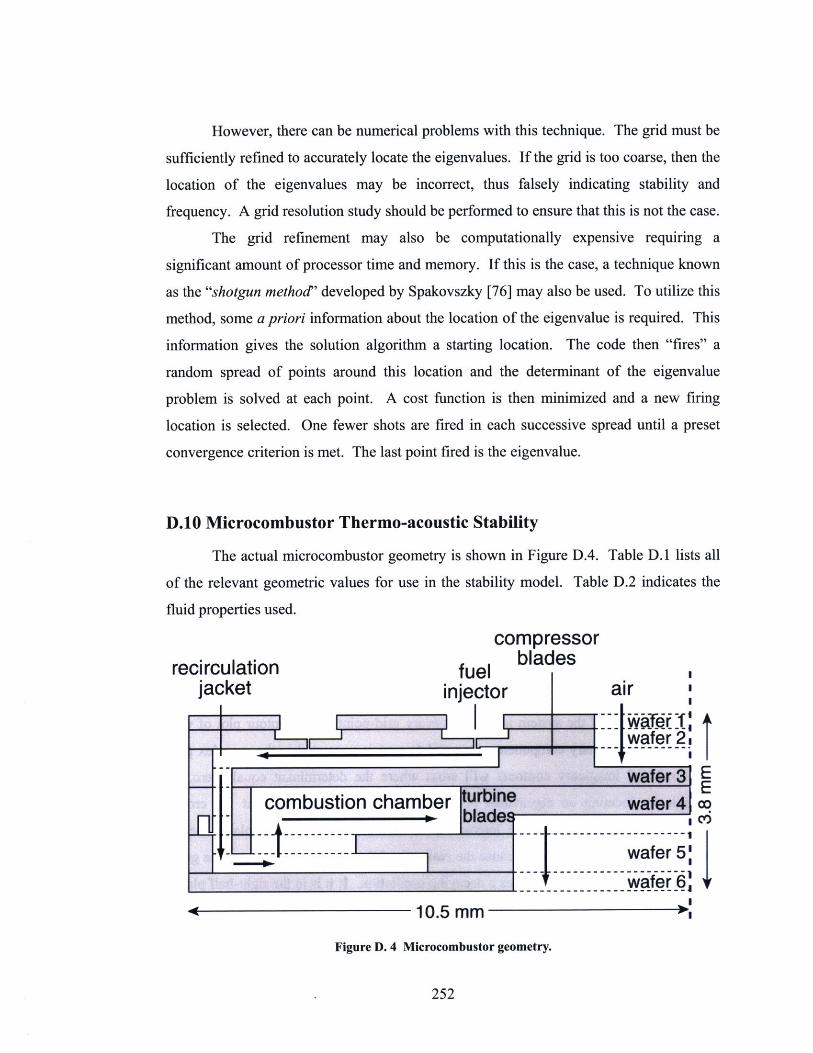
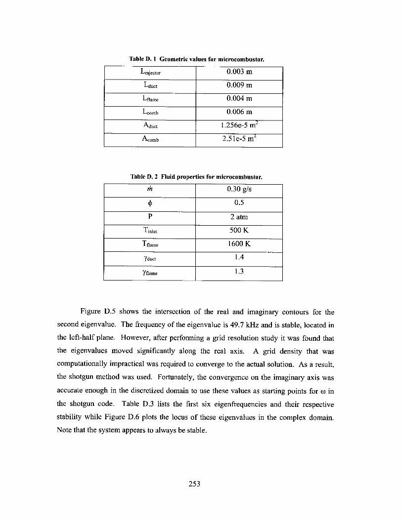
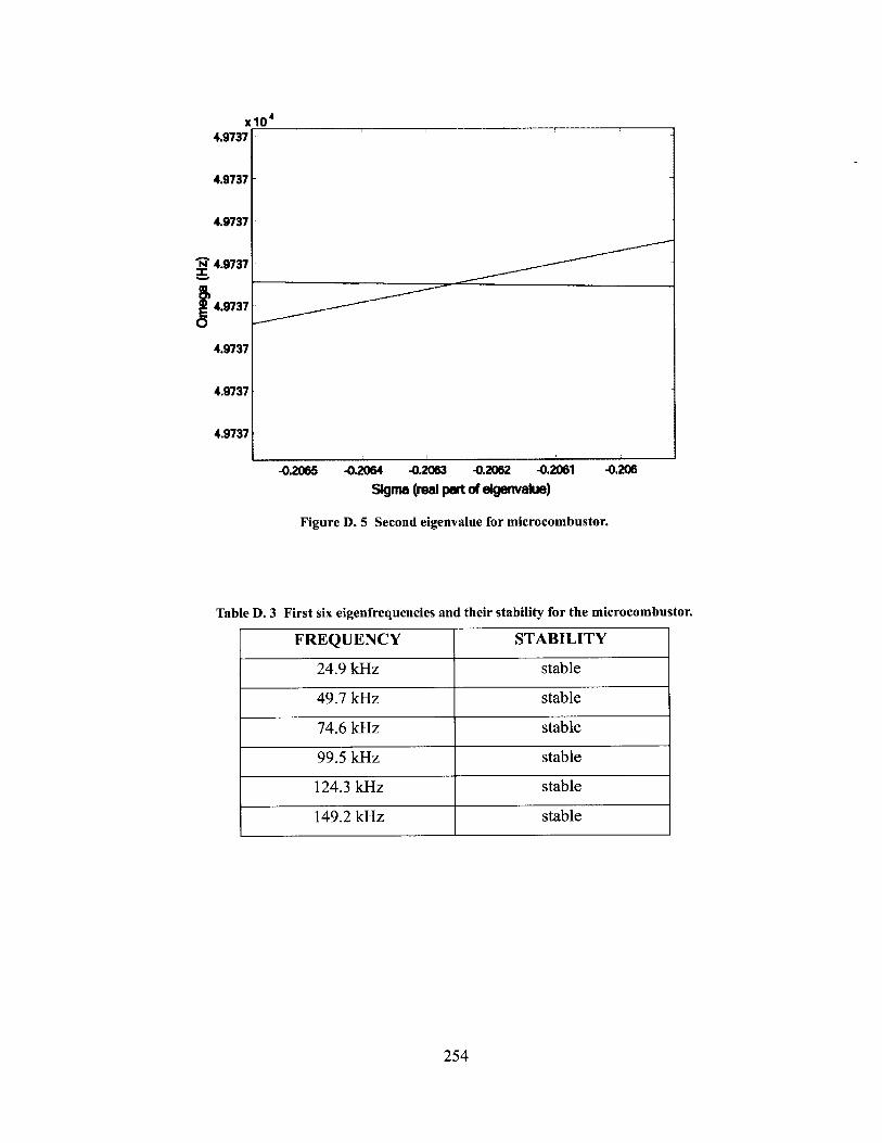
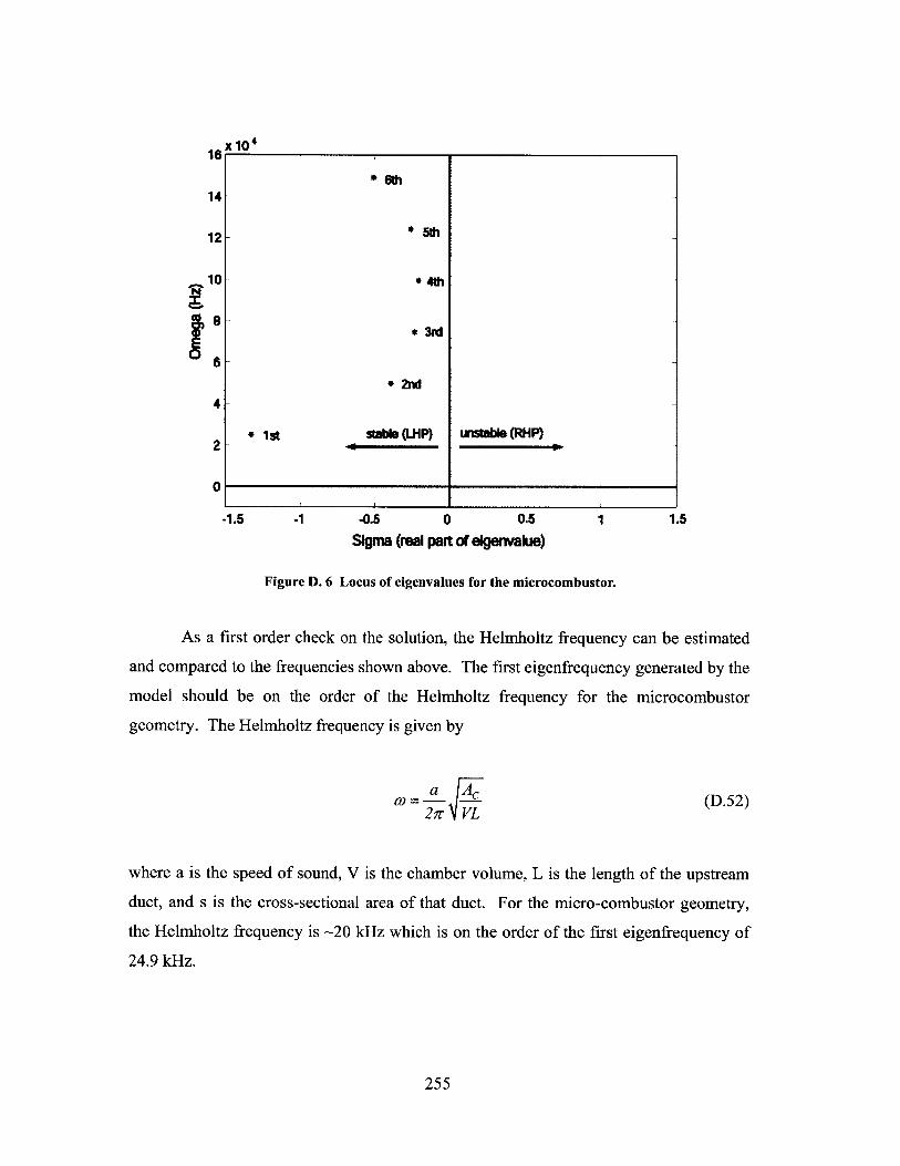
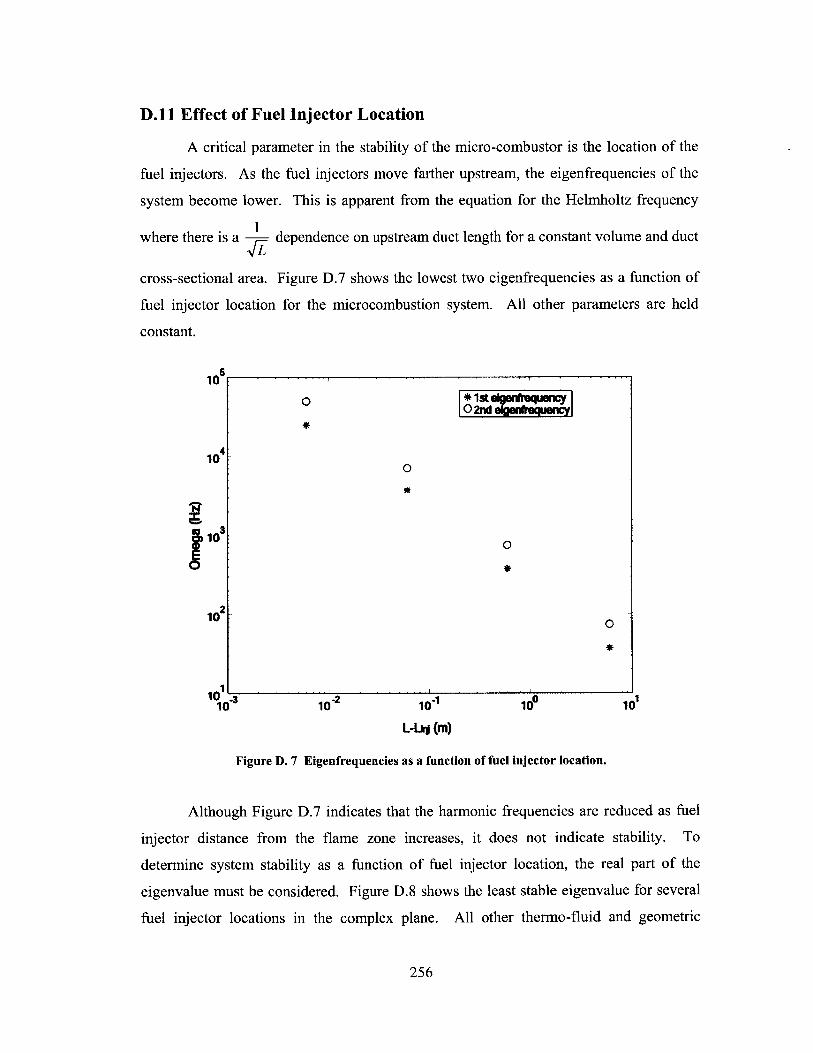
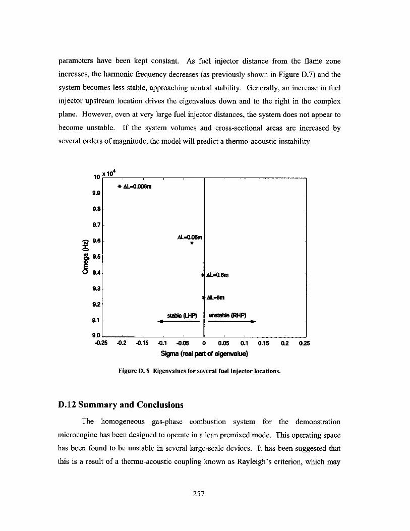
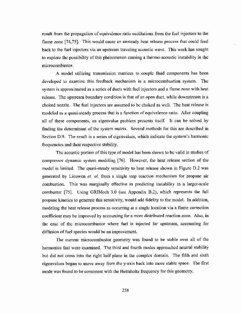
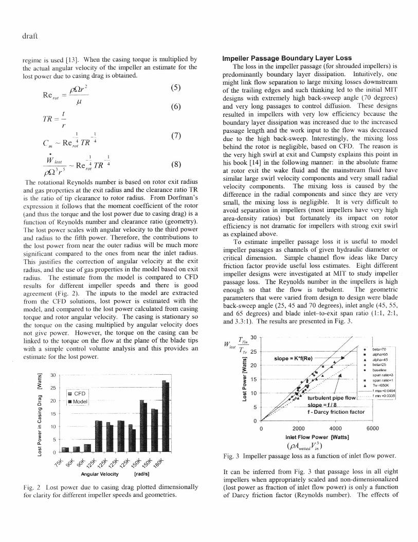
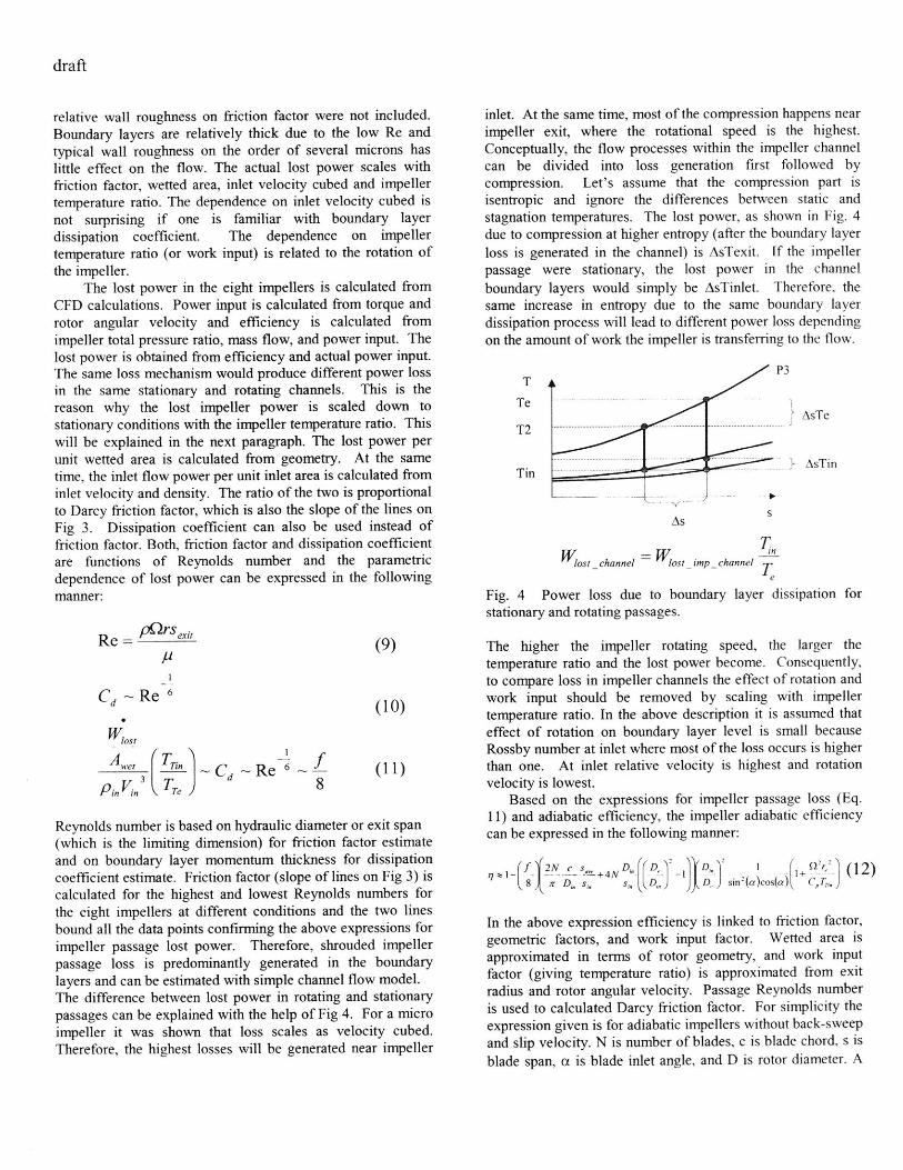
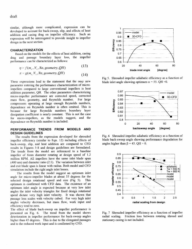
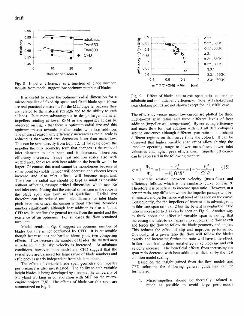
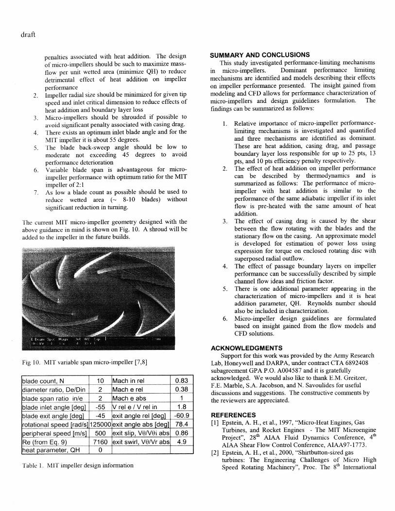
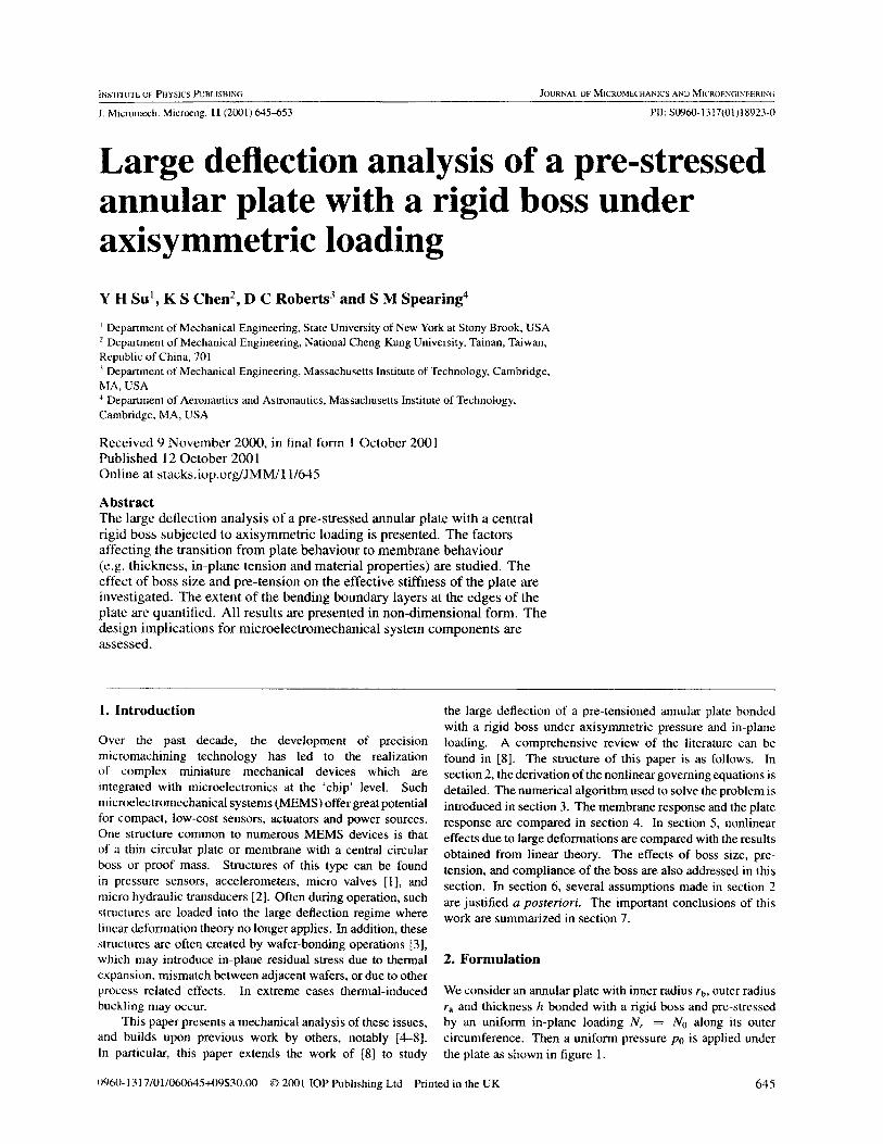
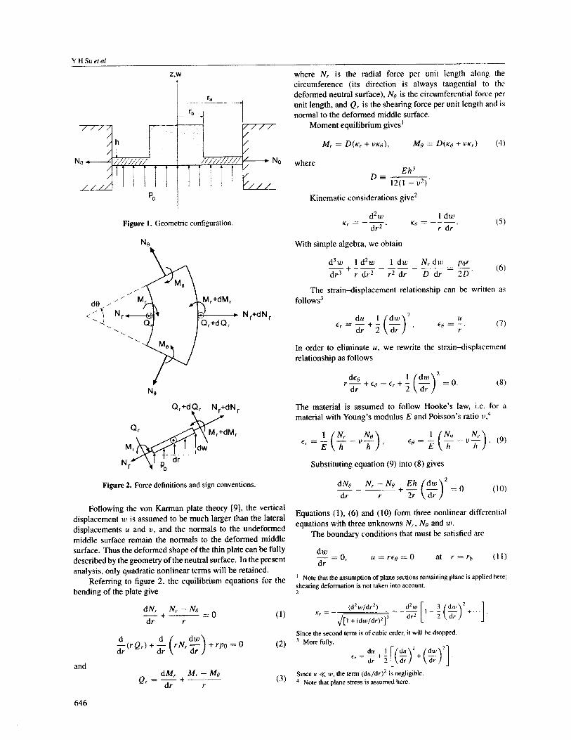
653


Recommended