Jussi Salmi, Andreas Richter, and Visa Koivunen. Sequential Unfolding SVD fortensors with applications in array signal processing. IEEE Transactions on SignalProcessing, accepted for publication.
This material is posted here with permission of the IEEE. Such permission of the IEEEdoes not in any way imply IEEE endorsement of any of Helsinki University ofTechnology's products or services. Internal or personal use of this material is permitted.However, permission to reprint/republish this material for advertising or promotionalpurposes or for creating new collective works for resale or redistribution must beobtained from the IEEE by writing to pubs[email protected].
By choosing to view this document, you agree to all provisions of the copyright lawsprotecting it.
Sequential Unfolding SVD for Tensors withApplications in Array Signal Processing
Jussi Salmi, Student Member, IEEE, Andreas Richter, Senior Member, IEEE, VisaKoivunen, Senior Member, IEEE
Abstract—This paper contributes to the field of higher order(N > 2) tensor decompositions in signal processing. A novelPARATREE tensor model is introduced, accompanied with Se-quential Unfolding SVD (SUSVD) algorithm. SUSVD, as thename indicates, applies a matrix singular value decompositionsequentially on the unfolded tensor reshaped from the righthand basis vectors of the SVD of the previous mode. Theconsequent PARATREE model is related to the well known familyof PARAFAC [1] tensor decomposition models. Both of themdescribe a tensor as a sum of rank-1 tensors, but PARATREE hasseveral advantages over PARAFAC, when it is applied as a lowerrank approximation technique. PARATREE is orthogonal (dueto SUSVD), fast and reliable to compute, and the order (or rank)of the decomposition can be adaptively adjusted. The low rankPARATREE approximation can be applied for, e.g., reducingcomputational complexity in inverse problems, measurementnoise suppression as well as data compression. The benefits of theproposed algorithm are illustrated through application examplesin signal processing in comparison to PARAFAC and HOSVD.
Index Terms—array signal processing, channel modeling, lowrank approximation, MIMO, SVD, tensor decompositions
I. INTRODUCTION
A tensor is any N -dimensional collection of data (asecond order tensor N = 2 is a matrix). In many
signal processing applications, instrumental data contains in-formation in more than two dimensions. Recently, researchersin several application areas have contributed to extendingwell established matrix operations to their tensor equivalents.Unfortunately, these extensions from their matrix counterpartsare not trivial. For instance, even though the Singular ValueDecomposition (SVD) has proven to be a powerful tool foranalyzing second order tensors (matrices), its generalization tohigher order tensors is not straightforward. There are severalapproaches for doing this, and none of them is superior in allaspects. In practice there are two major classes of models forhigher order tensor decomposition, namely Tucker-model [2]and PARAFAC (parallel factorization [1], [3]). The latter is
The research is partially funded by NORDITE WILATI project. The firstauthor would like to thank Finnish Technology Promotion Foundation (TES),Emil Aaltonen Foundation, Finnish Society of Electronics Engineers (EIS),HPY Research Foundation, and Nokia Foundation for financial support.
J. Salmi and V. Koivunen are with Department of Signal Processing andAcoustics, Helsinki University of Technology/SMARAD CoE, Espoo, Finland(e-mail: [email protected]).
A. Richter was with Department of Signal Processing and Acous-tics, Helsinki University of Technology/SMARAD CoE, Espoo, Finland.He is now with Nokia Research Center, Helsinki, Finland (e-mail: [email protected]).
also known as CANDECOMP (canonical decomposition [4]).PARAFAC-based tensor decomposition stem from multilinearanalysis in the fields of psychometrics [2], [5], sociology,chromatography and chemometrics [6]. It has been appliedin many signal processing applications, such as image recog-nition, acoustics, wireless channel estimation [7] and arraysignal processing [8], [9]. Recently, also a Tucker-modelbased HOSVD (Higher Order SVD) [10] tensor decompositionsubspace technique has been formulated to improve multidi-mensional harmonic retrieval problems [11]. In addition, thePARAFAC and HOSVD have been represented in an unifiedmanner in a general framework in [12].
In this paper a novel tensor model is introduced, whichbelongs to the class of PARAFAC techniques. The new model,referred to as PARATREE, has a distinct hierarchical treestructure. The key idea is to sequentially unfold the tensor(reshape into a matrix), and to apply the singular value decom-position (SVD) on this matrix. This procedure is repeated forthe right-hand singular vectors until no more data dimensionsremain encompassed in them. As a result, a hierarchical treestructure for the factors is formed (see Section II-D for details).In the following, this decomposition method will be referredto as Sequential Unfolding SVD (SUSVD).
The formulation of a tensor decomposition as a sum of rank-1 tensors (as in PARAFAC) is suitable for several applications.By additionally imposing the rank-1 terms of the decom-position to be orthogonal — a property which is inherentin the SUSVD — the PARATREE model can be efficientlyapplied to approximate higher-order (N > 2) tensors. Oneexample of such application involves interpreting the vectorof eigenvalues of a large covariance matrix as a tensor, whichis then used in a linear algebraic expression for finding theFisher Information Matrix. Approximating this tensor usingPARATREE decomposition allows for a significant reductionin computational complexity over a straight-forward matrixmultiplication or any other exact solution. PARATREE alsoachieves a significant complexity reduction against HOSVDand PARAFAC. However, the use of PARATREE in practiceis far more convenient than PARAFAC since the SUSVD doesnot suffer from convergence problems. Also the order of thePARATREE decomposition can be easily controlled, and thecorresponding approximation error is well defined.
In a second novel application the PARATREE model isapplied to suppress measurement noise in multidimensionalMIMO radio channel measurements. This is performed byidentifying the PARATREE components spanning the noisesubspace, and removing their contribution from the channel
2
observation.To summarize, the benefits of the proposed PARATREE
method include:• Reduced computational complexity in high dimensional
inverse problems• Measurement noise suppression (subspace filtering)• Compression of data (similar to low rank matrix approx-
imation)• Fast and reliable computation and adaptive order (rank)
selection• Revealing of hidden structures and dependencies in data.The paper is structured as follows. In Section II a brief
introduction to tensor modeling is provided along with thePARATREE description. Section III introduces the SUSVDand the PARATREE approximation for tensors. In Section IVtwo example applications are introduced in the field of arraysignal processing. Section V contains results for applying thealgorithm on real world data and comparing the performanceagainst PARAFAC and HOSVD approaches.
The notation used throughout the paper is as follows:• Calligraphic uppercase letters (A) denote higher order
(N > 2) tensors.• Boldface upper case letters (Roman A or Greek Σ)
denote matrices and lower case (a, σ) denote (column)vectors.
• The vector ai = (A)i denotes the ith column of a matrixA and the scalar aj = (a)j denotes the jth element of avector a.
• Non-boldface upper case letters (N ) denote constants,and lower case (a) denote scalar variables.
• Superscripts ∗, T, H, and + denote complex conjugate,matrix transpose, Hermitian (complex conjugate) trans-pose, and Moore-Penrose pseudo inverse, respectively.
• Different multiplication operators are defined for Kro-necker ⊗, Schur (elementwise) , Khatri-Rao ♦, outer, and n-mode ×n products, respectively.
• Symbol A denotes an estimate of the tensor A.• Operation vec(•) stacks all the elements
of the input tensor into a column vector.Operations diag(•), reshape(•, M1, . . . ,MN)(inverse of vec), permute(•, j1, . . . , jN), andipermute(•, j1, . . . , jN) (inverse of permute) aredefined as in MATLAB computing software [13].
• The Frobenius norm of a tensor is defined as
||A||F =
(∑i
∣∣∣(vec(A))
i
∣∣∣2) 12
=√
vec(A)Hvec(A).
II. TENSOR DECOMPOSITIONS
There are two major families of approaches to form atensor decomposition, namely the PARAFAC [1], [3] (CAN-DECOMP [4]) and the TUCKER [2] models. PARAFACis based on modeling the N -mode tensor as a sum of Rrank-1 tensors, whereas the TUCKER model decomposes atensor using a (smaller dimensional) core tensor and (possiblyorthonormal) basis matrices for each mode. A good description
of the properties and differences of the two approaches canbe found in e.g. [14], [15]. In general, PARAFAC modelinghas a more intuitive interpretation with common instrumentaldata, as the data can be often uniquely decomposed intoindividual contributions. Therefore, owing to its uniquenessproperties [1], [3], [8], [16], [17], PARAFAC modeling iscommonly used for signal modeling and estimation purposes,whereas orthogonal models such as HOSVD are better suitedfor tensor approximation, data compression, and filtering ap-plications.
A. Basic Tensor OperationsIn order to ensure the clarity of the notation, some tensor
terminology is introduced in the following. The term N -mode(or N -way) tensor can be used to describe any N -dimensionaldata structure. A factor is an individual rank-1 contributionused in forming the tensor decomposition. It is a successiveouter product of basis vectors (one from each mode), yieldinga rank-1 contribution to the tensor. The term rank refers to theminimum number of rank-1 components yielding the tensorin linear combination. Further discussion on tensor rank canbe found in [18], [19].
In the following some basic operations for an N-dimensionaltensor X ∈ CM1×...×Mn×...×MN are defined.
Definition 1 (The n-mode matrix unfolding): The n-modematrix unfolding X(n) of a tensor X comprises of:
1) Permutation of the tensor dimensions into an ordern, n+ 1, . . . , N, 1, . . . , n− 1.
2) Reshaping the permuted tensor into a matrix X(n) ∈CMn×
∏i6=n Mi , i.e.,
X(n) = reshape(permute(X , n, n+ 1, . . . , N, 1, . . . , n− 1), Mn,
∏i 6=n
Mi). (1)
The order in which the columns of the matrix after unfoldingare chosen in the latter step is not important, as long as the or-der is known and remains constant throughout the calculations.A more general treatment of the unfolding (or matricization),including nesting of several modes in the matrix rows, is givenin [20].
Definition 2 (The n-mode product): The n-mode productX ×n U ∈ CM1×...×Rn×...×MN of a tensor X and a matrixU ∈ CRn×Mn is defined as
X ×n U = ipermute (XU , n, n+ 1, . . . , N, 1, . . . , n− 1) ,(2)
Definition 3 (Rank-1 tensors and vector outer product): Atensor X is rank-1 if it can be expressed as an outer productof N vectors as
X = a(1) . . . a(N). (3)
The elements of X are then defined as
xm1m2...mN=
N∏n=1
(a(n))mn = a(1)m1· a(2)
m2· . . . · a(N)
mN(4)
3
B. PARAFAC Model
The PARAFAC model is essentially a description of thetensor as a sum of R rank-1 tensors. There are a numberof ways to express a PARAFAC decomposition [14], [15].Consider an N-mode tensor X ∈ CM1×M2×···×MN and Nmatrices A(n) ∈ CMn×R, where R is the number of factors— ideally equal to the rank of the tensor. Then the matricesA(n), n ∈ [1, . . . , N ], with columns a(n)
r , r ∈ [1, . . . , R] canbe formed such that the tensor X is the sum of outer products
X =R∑
r=1
a(1)r a(2)
r · · · a(N)r , (5)
where each outer product of the vectors a(n)r is a rank-1 tensor.
Equivalently, the PARAFAC model can be expressed element-wise as
xm1,m2,··· ,mN=
R∑r=1
a(1)r,m1· a(2)
r,m2· · · · · a(N)
r,mN, (6)
where mi denotes the index in ith mode. A vectorized defini-tion is given by
vec (X ) =(A(N)♦ · · ·♦A(1)
)1R =
R∑r=1
a(N)r ⊗ · · · ⊗ a(1)
r ,
(7)where 1R is a column vector of R ones.
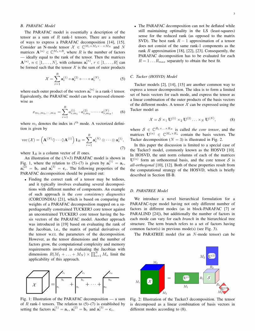
An illustration of the (N=3) PARAFAC model is shown inFig. 1, where the relation to (5)–(7) is given by a(1)
r = ar,a(2)
r = br and a(3)r = cr. The following properties of the
PARAFAC decomposition should be pointed out:• Finding the correct rank of a tensor may be tedious,
and it typically involves evaluating several decomposi-tions with different number of components. An exampleof such approach is the core consistency diagnostics(CORCONDIA) [21], which is based on comparing theweights of a PARAFAC decomposition mapped on a su-perdiagonally constrained TUCKER3 core tensor againstan unconstrained TUCKER3 core tensor having the ba-sis vectors of the PARAFAC model. Another approachwas introduced in [19] based on evaluating the rank ofthe Jacobian, i.e., the matrix of partial derivatives ofthe tensor w.r.t. the parameters of the decomposition.However, as the tensor dimensions and the number offactors grow, the computational complexity and memoryrequirements involved in evaluating the Jacobian withdimensions R(M1 + . . . + MN ) × ∏N
n=1Mn limit theapplicability of this approach.
X = + · · ·+ +b2
c2
a2
b1
a1
c1
bR
cR
aR
Fig. 1: Illustration of the PARAFAC decomposition — a sumof R rank-1 tensors. The relation to (5)–(7) is established bysetting the factors a(1)
r = ar, a(2)r = br and a(3)
r = cr.
• The PARAFAC decomposition can not be deflated whilestill maintaining optimality in the LS (least-squares)sense for the reduced rank (as opposed to the matrixSVD). The best rank R − 1 approximation of a tensordoes not consist of the same rank-1 components as therank R approximation [18], [22], [23]. Consequently, thePARAFAC decomposition has to be evaluated for eachR = 1 . . . Rmax separately to obtain the best fit.
C. Tucker (HOSVD) Model
Tucker models [2], [14], [15] are another common way toexpress a tensor decomposition. The idea is to form a limitedset of basis vectors for each mode, and express the tensor asa linear combination of the outer products of the basis vectorsof the different modes. A tensor X can be expressed using theTucker model as
X = S ×1 U(1) ×2 U(2) . . .×N U(N), (8)
where S ∈ CR1×...×RN is called the core tensor, and thematrices U(n) ∈ CMn×Rn contain the basis vectors. TheTucker decomposition (N = 3) is illustrated in Fig. 2.
In this paper the discussion is limited to a special case ofthe Tucker3 model, commonly known as the HOSVD [10].In HOSVD, the unit norm columns of each of the matricesU(n) form an orthonormal basis, and the core tensor S isall-orthogonal [10], [12]. Both of these properties result fromthe computational strategy of the HOSVD, which is brieflydescribed in Section III-B.
D. PARATREE Model
We introduce a novel hierarchical formulation for aPARAFAC-type model having not only different number offactors in different modes (as in block-PARAFAC [7] orPARALIND [24]), but additionally the number of factors ineach mode can vary for each branch in the hierarchical treestructure. The term branch refers to a set of factors havingcommon factor(s) in previous mode(s) (see Fig. 3).
The PARATREE model (for an N -mode tensor) can be
M3
M1
R1
R3
M3
M2
R2
M2
M1
S=X
U(2)
U(3)
U(1)
Fig. 2: Illustration of the Tucker3 decomposition. The tensoris decomposed as a linear combination of basis vectors indifferent modes according to (8).
4
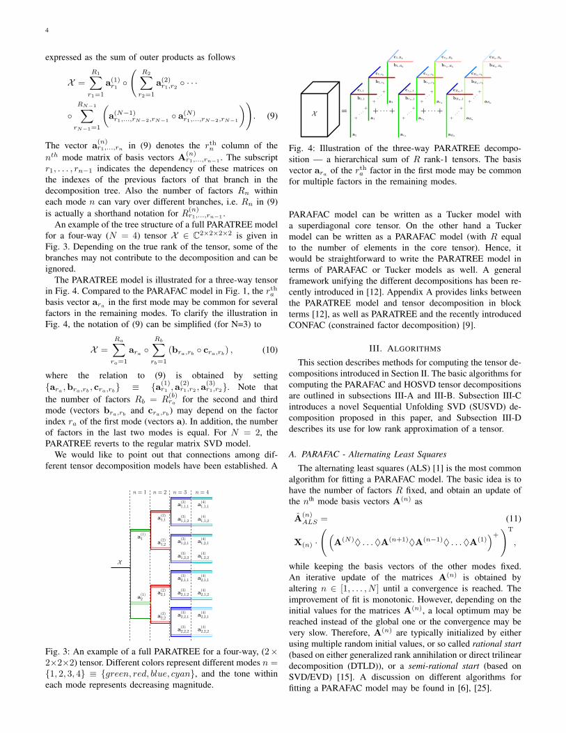
expressed as the sum of outer products as follows
X =R1∑
r1=1
a(1)r1(
R2∑r2=1
a(2)r1,r2
· · ·
RN−1∑
rN−1=1
(a(N−1)
r1,...,rN−2,rN−1 a(N)
r1,...,rN−2,rN−1
)). (9)
The vector a(n)r1,...,rn in (9) denotes the rthn column of the
nth mode matrix of basis vectors A(n)r1,...,rn−1 . The subscript
r1, . . . , rn−1 indicates the dependency of these matrices onthe indexes of the previous factors of that branch in thedecomposition tree. Also the number of factors Rn withineach mode n can vary over different branches, i.e. Rn in (9)is actually a shorthand notation for R(n)
r1,...,rn−1 .An example of the tree structure of a full PARATREE model
for a four-way (N = 4) tensor X ∈ C2×2×2×2 is given inFig. 3. Depending on the true rank of the tensor, some of thebranches may not contribute to the decomposition and can beignored.
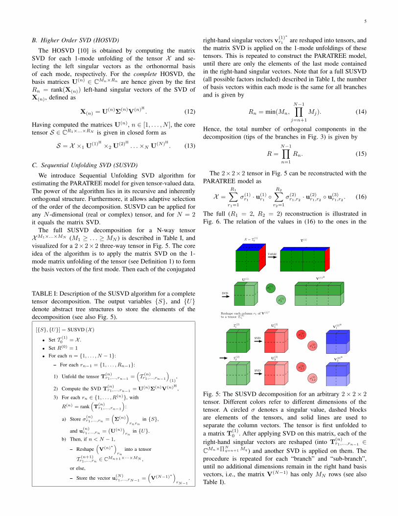
The PARATREE model is illustrated for a three-way tensorin Fig. 4. Compared to the PARAFAC model in Fig. 1, the rthabasis vector ara
in the first mode may be common for severalfactors in the remaining modes. To clarify the illustration inFig. 4, the notation of (9) can be simplified (for N=3) to
X =Ra∑
ra=1
ara Rb∑
rb=1
(bra,rb cra,rb
) , (10)
where the relation to (9) is obtained by settingara
,bra,rb, cra,rb
≡ a(1)r1 ,a
(2)r1,r2 ,a
(3)r1,r2. Note that
the number of factors Rb = R(b)ra for the second and third
mode (vectors bra,rband cra,rb
) may depend on the factorindex ra of the first mode (vectors a). In addition, the numberof factors in the last two modes is equal. For N = 2, thePARATREE reverts to the regular matrix SVD model.
We would like to point out that connections among dif-ferent tensor decomposition models have been established. A
a(4)1,1,1
n = 3n = 2n = 1
a(2)2,1
a(3)2,1,1
a(3)2,1,2 a
(4)2,1,2
a(4)2,1,1
a(2)2,2
a(4)2,2,2
a(4)2,2,1a
(3)2,2,1
a(3)2,2,2
a(1)2
a(1)1
a(4)1,2,2
a(3)1,2,1
a(3)1,2,2
a(4)1,2,1
X
a(2)1,1
a(2)1,2
a(3)1,1,1
a(3)1,1,2 a
(4)1,1,2
n = 4
Fig. 3: An example of a full PARATREE for a four-way, (2×2×2×2) tensor. Different colors represent different modes n =1, 2, 3, 4 ≡ green, red, blue, cyan, and the tone withineach mode represents decreasing magnitude.
+
· · ·+
+
· ··+
+
· · ·+
+
· ··+
+
· · ·+
+X =
bRa,Rb
bRa,rb
bRa,1
bra,Rb
bra,rb
bra,1
b1,Rb
b1,rb
b1,1
c1,rb
c1,1 cra,1
cra,rb
cra,Rbc1,Rb cRa,Rb
cRa,rb
cRa,1
a1 ara aRa
aRa
aRaara
ara
a1
· · ·a1
++ · · ·++
· ··+
Fig. 4: Illustration of the three-way PARATREE decompo-sition — a hierarchical sum of R rank-1 tensors. The basisvector ara
of the rtha factor in the first mode may be commonfor multiple factors in the remaining modes.
PARAFAC model can be written as a Tucker model witha superdiagonal core tensor. On the other hand a Tuckermodel can be written as a PARAFAC model (with R equalto the number of elements in the core tensor). Hence, itwould be straightforward to write the PARATREE model interms of PARAFAC or Tucker models as well. A generalframework unifying the different decompositions has been re-cently introduced in [12]. Appendix A provides links betweenthe PARATREE model and tensor decomposition in blockterms [12], as well as PARATREE and the recently introducedCONFAC (constrained factor decomposition) [9].
III. ALGORITHMS
This section describes methods for computing the tensor de-compositions introduced in Section II. The basic algorithms forcomputing the PARAFAC and HOSVD tensor decompositionsare outlined in subsections III-A and III-B. Subsection III-Cintroduces a novel Sequential Unfolding SVD (SUSVD) de-composition proposed in this paper, and Subsection III-Ddescribes its use for low rank approximation of a tensor.
A. PARAFAC - Alternating Least Squares
The alternating least squares (ALS) [1] is the most commonalgorithm for fitting a PARAFAC model. The basic idea is tohave the number of factors R fixed, and obtain an update ofthe nth mode basis vectors A(n) as
A(n)ALS = (11)
X(n) ·((
A(N)♦ . . .♦A(n+1)♦A(n−1)♦ . . .♦A(1))+)T
,
while keeping the basis vectors of the other modes fixed.An iterative update of the matrices A(n) is obtained byaltering n ∈ [1, . . . , N ] until a convergence is reached. Theimprovement of fit is monotonic. However, depending on theinitial values for the matrices A(n), a local optimum may bereached instead of the global one or the convergence may bevery slow. Therefore, A(n) are typically initialized by eitherusing multiple random initial values, or so called rational start(based on either generalized rank annihilation or direct trilineardecomposition (DTLD)), or a semi-rational start (based onSVD/EVD) [15]. A discussion on different algorithms forfitting a PARAFAC model may be found in [6], [25].
5
B. Higher Order SVD (HOSVD)
The HOSVD [10] is obtained by computing the matrixSVD for each 1-mode unfolding of the tensor X and se-lecting the left singular vectors as the orthonormal basisof each mode, respectively. For the complete HOSVD, thebasis matrices U(n) ∈ CMn×Rn are hence given by the firstRn = rank(X(n)) left-hand singular vectors of the SVD ofX(n), defined as
X(n) = U(n)Σ(n)V(n)H . (12)
Having computed the matrices U(n), n ∈ [1, . . . , N ], the coretensor S ∈ CR1×...×RN is given in closed form as
S = X ×1 U(1)H ×2 U(2)H . . .×N U(N)H . (13)
C. Sequential Unfolding SVD (SUSVD)
We introduce Sequential Unfolding SVD algorithm forestimating the PARATREE model for given tensor-valued data.The power of the algorithm lies in its recursive and inherentlyorthogonal structure. Furthermore, it allows adaptive selectionof the order of the decomposition. SUSVD can be applied forany N -dimensional (real or complex) tensor, and for N = 2it equals the matrix SVD.
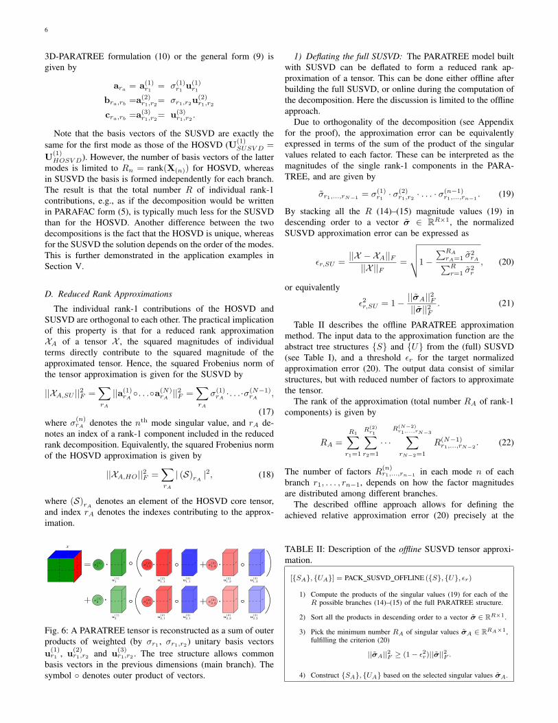
The full SUSVD decomposition for a N-way tensorXM1×...×MN (M1 ≥ . . . ≥ MN ) is described in Table I, andvisualized for a 2×2×2 three-way tensor in Fig. 5. The coreidea of the algorithm is to apply the matrix SVD on the 1-mode matrix unfolding of the tensor (see Definition 1) to formthe basis vectors of the first mode. Then each of the conjugated
TABLE I: Description of the SUSVD algorithm for a completetensor decomposition. The output variables S, and Udenote abstract tree structures to store the elements of thedecomposition (see also Fig. 5).
[S, U] = SUSVD (X )
• Set T (1)0 = X .
• Set R(0) = 1
• For each n = 1, . . . , N − 1:– For each rn−1 = 1, . . . , Rn−1:
1) Unfold the tensor T(n)r1,...,rn−1 =
(T (n)
r1,...,rn−1
)(1)
,
2) Compute the SVD T(n)r1,...,rn−1 = U(n)Σ(n)V(n)H ,
3) For each rn ∈ 1, . . . , R(n), with
R(n) = rank(T
(n)r1,...,rn−1
):
a) Store σ(n)r1,...,rn =
(Σ(n)
)rnrn
in S,
and u(n)r1,...,rn =
(U(n)
)rn
in U.b) Then, if n < N − 1,
– Reshape(V(n)∗
)rn
into a tensor
T (n+1)r1,...,rn ∈ CMn+1×···×MN ,
or else,
– Store the vector u(N)r1,...,rN−1 =
(V(N−1)∗
)rN−1
.
right-hand singular vectors v(1)∗r1 are reshaped into tensors, and
the matrix SVD is applied on the 1-mode unfoldings of thesetensors. This is repeated to construct the PARATREE model,until there are only the elements of the last mode containedin the right-hand singular vectors. Note that for a full SUSVD(all possible factors included) described in Table I, the numberof basis vectors within each mode is the same for all branchesand is given by
Rn = min(Mn,
N−1∏j=n+1
Mj). (14)
Hence, the total number of orthogonal components in thedecomposition (tips of the branches in Fig. 3) is given by
R =N−1∏n=1
Rn. (15)
The 2×2×2 tensor in Fig. 5 can be reconstructed with thePARATREE model as
X =R1∑
r1=1
σ(1)r1· u(1)
r1
R2∑r2=1
σ(2)r1,r2
· u(2)r1,r2
u(3)r1,r2
. (16)
The full (R1 = 2, R2 = 2) reconstruction is illustrated inFig. 6. The relation of the values in (16) to the ones in the
Unfold
SVD
SVD
SVD
T(1)X = T (1)0
T (2)2
Reshape each column r1 of V(1)∗
V(2)H
2
V(2)H
1
V(1)H
U(1)
σ(1)1
σ(1)2
U(2)1
σ(2)1,2
σ(2)1,1
to a tensor T (2)r1
U(2)2
σ(2)2,1
σ(2)2,2
T (2)1
Fig. 5: The SUSVD decomposition for an arbitrary 2× 2× 2tensor. Different colors refer to different dimensions of thetensor. A circled σ denotes a singular value, dashed blocksare elements of the tensors, and solid lines are used toseparate the column vectors. The tensor is first unfolded toa matrix T(1)
0 . After applying SVD on this matrix, each of theright-hand singular vectors are reshaped (into T(n)
r1,...,rn−1 ∈CMn×
∏Nq=n+1 Mq ) and another SVD is applied on them. The
procedure is repeated for each “branch” and “sub-branch”,until no additional dimensions remain in the right hand basisvectors, i.e., the matrix V(N−1) has only MN rows (see alsoTable I).
6
3D-PARATREE formulation (10) or the general form (9) isgiven by
ara= a(1)
r1= σ(1)
r1u(1)
r1
bra,rb=a(2)
r1,r2= σr1,r2u
(2)r1,r2
cra,rb=a(3)
r1,r2= u(3)
r1,r2.
Note that the basis vectors of the SUSVD are exactly thesame for the first mode as those of the HOSVD (U(1)
SUSV D =U(1)
HOSV D). However, the number of basis vectors of the lattermodes is limited to Rn = rank(X(n)) for HOSVD, whereasin SUSVD the basis is formed independently for each branch.The result is that the total number R of individual rank-1contributions, e.g., as if the decomposition would be writtenin PARAFAC form (5), is typically much less for the SUSVDthan for the HOSVD. Another difference between the twodecompositions is the fact that the HOSVD is unique, whereasfor the SUSVD the solution depends on the order of the modes.This is further demonstrated in the application examples inSection V.
D. Reduced Rank Approximations
The individual rank-1 contributions of the HOSVD andSUSVD are orthogonal to each other. The practical implicationof this property is that for a reduced rank approximationXA of a tensor X , the squared magnitudes of individualterms directly contribute to the squared magnitude of theapproximated tensor. Hence, the squared Frobenius norm ofthe tensor approximation is given for the SUSVD by
||XA,SU ||2F =∑rA
||a(1)rA. . .a(N)
rA||2F =
∑rA
σ(1)rA·. . .·σ(N−1)
rA,
(17)where σ(n)
rA denotes the nth mode singular value, and rA de-notes an index of a rank-1 component included in the reducedrank decomposition. Equivalently, the squared Frobenius normof the HOSVD approximation is given by
||XA,HO||2F =∑rA
| (S)rA|2, (18)
where (S)rAdenotes an element of the HOSVD core tensor,
and index rA denotes the indexes contributing to the approx-imation.
σ(2)1,1=
X
σ(1)1 +
u(1)1
u(1)2
u(2)1,1 u
(2)1,2u
(3)1,1 u
(3)1,2
u(3)2,1 u
(3)2,2u
(2)2,2u
(2)2,1
+ +σ(1)2 σ
(2)2,1
σ(2)1,2
σ(2)2,2
Fig. 6: A PARATREE tensor is reconstructed as a sum of outerproducts of weighted (by σr1 , σr1,r2 ) unitary basis vectorsu(1)
r1 , u(2)r1,r2 and u(3)
r1,r2 . The tree structure allows commonbasis vectors in the previous dimensions (main branch). Thesymbol denotes outer product of vectors.
1) Deflating the full SUSVD: The PARATREE model builtwith SUSVD can be deflated to form a reduced rank ap-proximation of a tensor. This can be done either offline afterbuilding the full SUSVD, or online during the computation ofthe decomposition. Here the discussion is limited to the offlineapproach.
Due to orthogonality of the decomposition (see Appendixfor the proof), the approximation error can be equivalentlyexpressed in terms of the sum of the product of the singularvalues related to each factor. These can be interpreted as themagnitudes of the single rank-1 components in the PARA-TREE, and are given by
σr1,...,rN−1 = σ(1)r1· σ(2)
r1,r2· . . . · σ(n−1)
r1,...,rn−1. (19)
By stacking all the R (14)–(15) magnitude values (19) indescending order to a vector σ ∈ RR×1, the normalizedSUSVD approximation error can be expressed as
εr,SU =||X − XA||F||X ||F
=
√√√√1−∑RA
rA=1 σ2rA∑R
r=1 σ2r
, (20)
or equivalently
ε2r,SU = 1− ||σA||2F||σ||2F
. (21)
Table II describes the offline PARATREE approximationmethod. The input data to the approximation function are theabstract tree structures S and U from the (full) SUSVD(see Table I), and a threshold εr for the target normalizedapproximation error (20). The output data consist of similarstructures, but with reduced number of factors to approximatethe tensor.
The rank of the approximation (total number RA of rank-1components) is given by
RA =R1∑
r1=1
R(2)r1∑
r2=1
· · ·R(N−2)
r1,...,rN−3∑rN−2=1
R(N−1)r1,...,rN−2
. (22)
The number of factors R(n)r1,...,rn−1 in each mode n of each
branch r1, . . . , rn−1, depends on how the factor magnitudesare distributed among different branches.
The described offline approach allows for defining theachieved relative approximation error (20) precisely at the
TABLE II: Description of the offline SUSVD tensor approxi-mation.
[SA, UA] = PACK SUSVD OFFLINE (S, U, εr)
1) Compute the products of the singular values (19) for each of theR possible branches (14)–(15) of the full PARATREE structure.
2) Sort all the products in descending order to a vector σ ∈ RR×1.
3) Pick the minimum number RA of singular values σA ∈ RRA×1,fulfilling the criterion (20)
||σA||2F ≥ (1− ε2r)||σ||2F .
4) Construct SA, UA based on the selected singular values σA.
7
price of having to form the full SUSVD. This is most usefulwhen saving in the computational complexity of the SUSVDdecomposition itself is not crucial for the application at hand.This is the case in both of the example applications in Sec-tion IV. Further improvements in computational complexitycould be achieved by truncating the decomposition in anonline fashion, but then controlling the normalized error ofthe obtained approximation would not be as straightforward.
2) Deflating the full HOSVD: The HOSVD could be de-flated either by reducing the least significant basis vectors fromthe matrices U(n), or by considering the full decomposition,and selecting the elements from the core tensor that onewishes to include in the approximation. Here, the discussionis limited to the latter approach as that strategy for controllingthe approximation error is similar to the one applied for theSUSVD deflation. Hence, the deflation of the HOSVD isobtained by setting the undesired contributions in the coretensor to zero, yielding a sparse core tensor SA. The obtainedHOSVD approximation error is given by
ε2r,HO = 1− ||SA||2F||S||2F
. (23)
It should be noted that the low rank tensor approximationsobtained by deflation are suboptimal both for the SUSVD andthe HOSVD. However, in the proposed application example inSection IV-B, the optimality of the approximation in LS sensemay be sacrificed to the benefit of a computationally efficientmethod yielding an approximation with a low number of rank-1 factors in the decomposition (nonzero core tensor elementsfor HOSVD). For HOSVD, the truncation could be performedalso by reducing the rank of each mode, which would allowto further optimize the solution using Tucker3-ALS [14], [15],[26]. However, this method is time consuming, the achievableapproximation error would not be as precisely controllable,and the obtained decomposition may still contain numerousinsignificant rank-1 factors.
Applying a similar target approximation error requirementfor a general PARAFAC model would require a trial anderror approach for finding a proper rank (as well as fordetermining the tensor-rank in general). Also the convergenceof the alternating least squares (ALS [26]) algorithms used forPARAFAC is very slow for high dimensional or ill-conditionedproblems [27], [28].
IV. APPLICATION EXAMPLES
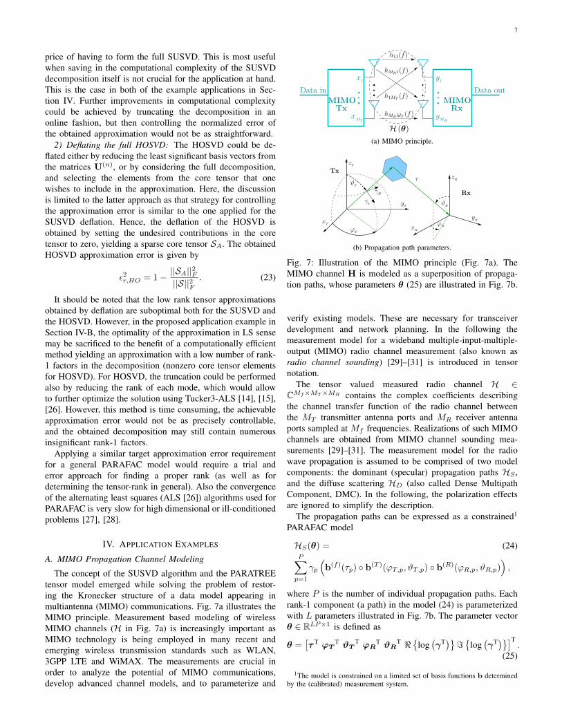
A. MIMO Propagation Channel Modeling
The concept of the SUSVD algorithm and the PARATREEtensor model emerged while solving the problem of restor-ing the Kronecker structure of a data model appearing inmultiantenna (MIMO) communications. Fig. 7a illustrates theMIMO principle. Measurement based modeling of wirelessMIMO channels (H in Fig. 7a) is increasingly important asMIMO technology is being employed in many recent andemerging wireless transmission standards such as WLAN,3GPP LTE and WiMAX. The measurements are crucial inorder to analyze the potential of MIMO communications,develop advanced channel models, and to parameterize and
hMRMT(f)
Data out
h11(f)
h1MT(f)
H (θ)
x1
Data in
xMT
MIMORx
MIMO
y1
yMR
hMR1(f)
Tx
(a) MIMO principle.
yT
xR
τ
yR
zR
zT
ϑR
ϕR
xT
Rx
ϕT
γV
γH
ϑT
Tx
(b) Propagation path parameters.
Fig. 7: Illustration of the MIMO principle (Fig. 7a). TheMIMO channel H is modeled as a superposition of propaga-tion paths, whose parameters θ (25) are illustrated in Fig. 7b.
verify existing models. These are necessary for transceiverdevelopment and network planning. In the following themeasurement model for a wideband multiple-input-multiple-output (MIMO) radio channel measurement (also known asradio channel sounding) [29]–[31] is introduced in tensornotation.
The tensor valued measured radio channel H ∈CMf×MT×MR contains the complex coefficients describingthe channel transfer function of the radio channel betweenthe MT transmitter antenna ports and MR receiver antennaports sampled at Mf frequencies. Realizations of such MIMOchannels are obtained from MIMO channel sounding mea-surements [29]–[31]. The measurement model for the radiowave propagation is assumed to be comprised of two modelcomponents: the dominant (specular) propagation paths HS ,and the diffuse scattering HD (also called Dense MultipathComponent, DMC). In the following, the polarization effectsare ignored to simplify the description.
The propagation paths can be expressed as a constrained1
PARAFAC model
HS(θ) = (24)P∑
p=1
γp
(b(f)(τp) b(T )(ϕT,p, ϑT,p) b(R)(ϕR,p, ϑR,p)
),
where P is the number of individual propagation paths. Eachrank-1 component (a path) in the model (24) is parameterizedwith L parameters illustrated in Fig. 7b. The parameter vectorθ ∈ RLP×1 is defined as
θ =[τ T ϕT
T ϑTT ϕR
T ϑRT <
log(γT)=log
(γT)]T
.(25)
1The model is constrained on a limited set of basis functions b determinedby the (calibrated) measurement system.
8
TABLE III: System dimensions in the complexity examples.Label Value
Frequency samples Mf 193Transmitter ports MT 30
Receiver ports MR 31Total Number of Parameters L′ 800
The parameters are delay (τ ), azimuth (ϕ) and elevation (ϑ)angles of departure (at Tx) and arrival (at Rx), and complexpath weights γ for each path. The vectors b(i)(θp) ∈ CMi×1,i ∈ f, T,R, θ ∈ τ, ϕT , ϑT , ϕR, ϑR in (24) de-note the basis functions for the frequency, transmit array,and receive array modes, respectively. The description ofthe mapping of the parameters within the basis functions israther lengthy, and hence omitted here. The interested readeris directed to [29], [32] for additional details on how theparameters characterize the channel. Parametric estimation of(24) is discussed in [29], [32]–[34].
The diffuse scattering component is defined as a tensorvalued complex circular symmetric normal distributed randomvariable
HD ∼ NC (0,RD) , (26)
with a covariance tensor R ∈ CMf×MT×MR×Mf×MT×MR .The following Kronecker structure is assumed for the covari-ance tensor reshaped into a (M ×M , with M = MfMTMR)matrix
RD = Evec(HD)vec(HD)H
= Rf⊗RT⊗RR ∈ CM×M .
(27)The matrices Rf ∈ CMf×Mf , RT ∈ CMT×MT , and RR ∈CMR×MR are the covariance matrices of the frequency, thetransmit array, and the receive array modes, respectively.Estimation of these covariance matrices is discussed in [35].
Furthermore, a tensor HN (k) is defined, denoting zeromean i.i.d. normal distributed complex circular symmetric(measurement) noise with covariance
RN = Evec(HN )vec(HN )H = σ2NI. (28)
Using (24), (26), and (28) the model for the full measuredcomplex transfer function of the radio channel tensor (asnapshot) at time k is defined as
H(k) = HS(k) +HD(k) +HN (k) ∼ NC (HS ,R) , (29)
where the covariance tensor is defined as R = RD +RN . Thecovariance tensor of (29) can be written in matrix form as
R = Evec(H)vec(H)H = Rf ⊗RT ⊗RR + σ2NI. (30)
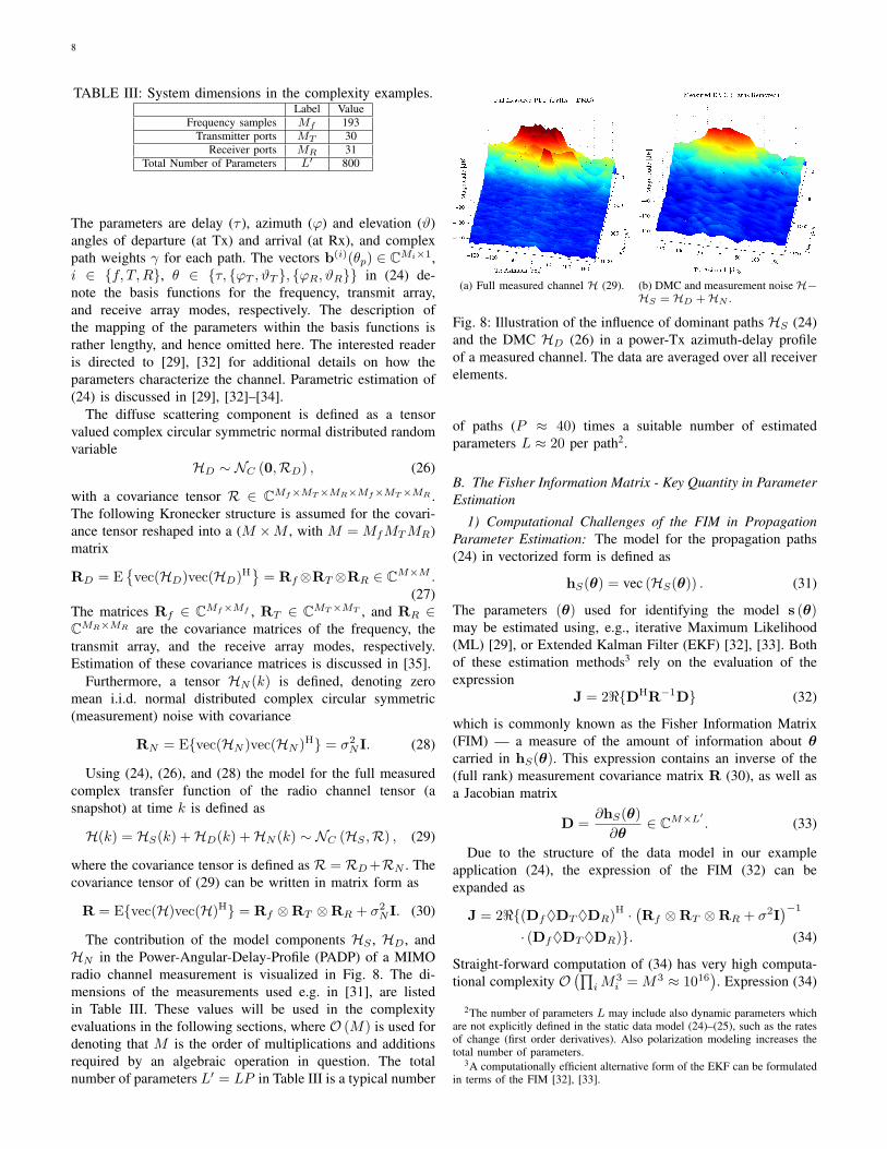
The contribution of the model components HS , HD, andHN in the Power-Angular-Delay-Profile (PADP) of a MIMOradio channel measurement is visualized in Fig. 8. The di-mensions of the measurements used e.g. in [31], are listedin Table III. These values will be used in the complexityevaluations in the following sections, where O (M) is used fordenoting that M is the order of multiplications and additionsrequired by an algebraic operation in question. The totalnumber of parameters L′ = LP in Table III is a typical number
(a) Full measured channel H (29). (b) DMC and measurement noiseH−HS = HD +HN .
Fig. 8: Illustration of the influence of dominant paths HS (24)and the DMC HD (26) in a power-Tx azimuth-delay profileof a measured channel. The data are averaged over all receiverelements.
of paths (P ≈ 40) times a suitable number of estimatedparameters L ≈ 20 per path2.
B. The Fisher Information Matrix - Key Quantity in ParameterEstimation
1) Computational Challenges of the FIM in PropagationParameter Estimation: The model for the propagation paths(24) in vectorized form is defined as
hS(θ) = vec (HS(θ)) . (31)
The parameters (θ) used for identifying the model s (θ)may be estimated using, e.g., iterative Maximum Likelihood(ML) [29], or Extended Kalman Filter (EKF) [32], [33]. Bothof these estimation methods3 rely on the evaluation of theexpression
J = 2<DHR−1D (32)
which is commonly known as the Fisher Information Matrix(FIM) — a measure of the amount of information about θcarried in hS(θ). This expression contains an inverse of the(full rank) measurement covariance matrix R (30), as well asa Jacobian matrix
D =∂hS(θ)∂θ
∈ CM×L′ . (33)
Due to the structure of the data model in our exampleapplication (24), the expression of the FIM (32) can beexpanded as
J = 2<(Df♦DT ♦DR)H ·(Rf ⊗RT ⊗RR + σ2I
)−1
· (Df♦DT ♦DR). (34)
Straight-forward computation of (34) has very high computa-tional complexity O
(∏iM
3i = M3 ≈ 1016
). Expression (34)
2The number of parameters L may include also dynamic parameters whichare not explicitly defined in the static data model (24)–(25), such as the ratesof change (first order derivatives). Also polarization modeling increases thetotal number of parameters.
3A computationally efficient alternative form of the EKF can be formulatedin terms of the FIM [32], [33].
9
also requires memory for storing the full matrix R ∈ CM×M
(and D ∈ CM×L′ ), resulting in the order of 600 GB (IEEEdouble precision) assuming the dimensions in Table III (M =MfMTMR = 197632, and L′ = 800).
To facilitate feasible computation of the FIM (32), thepositive definite covariance matrix R (30) can be expressedin terms of its eigenvalue decomposition as
and it requires storing the full matrix D (33). Let usreshape the diagonal elements of Λ−1 in (38) into a tensorL ∈ CMf×MT×MR as
L = reshape(diag
(Λ−1
), Mf ,MT ,MR
). (39)
This tensor is, in general, of full rank4. One feasible solutionfor computing the FIM (36) is then given by
Jo =2< Mf∑
mf =1
[d′Hfmf
d′fmf
MT∑mT =1
[d′HTmT
d′TmT
MR∑
mR=1
[lmf ,mT ,mR
· d′HRmRd′RmR
]]], (40)
where d′imi, i ∈ f, T,R, denotes the mth
i row of the matrixD′i in (37). Expression (40) is exact and does not requirestoring the full matrix D in (33), but has the same (high)computational complexity
O(L′
2∏
i
Mi ≈ 1011
)(41)
as (36).2) Applying Tensor Decompositions for Solving the FIM:
The PARATREE model can be applied to reduce the computa-tional complexity of (40). The tensor L in (39) is decomposedinto a PARATREE model with a single matrix of basis vectorsL(f) ∈ RMf×Rf for the f -mode, and Rf matrices L(T )
rf ∈RMT×RT and L(R)
rf ∈ RMR×RT for the T - and R-modes (see
4In [36] it is shown that if the term σ2I would not be present, L wouldbe a rank-1 tensor, and solving (36) becomes computationally attractive.
Table I for details). Then a PARATREE approximation JPT
for the FIM can be expressed as
JPT = 2< Rf∑
rf =1
[(D′Hf Λ(f)
rfD′f
)(42)
RT∑rT
[ (D′HT Λ(T )
rf ,rTD′T
)(D′HRdiagΛ(R)
rf ,rTD′R
) ]],
where Λ(R)rf ,rT
= diag((L(R)rf )rT
) denotes a diagonal matrixformed from the rthT column of L(R)
rf etc. This solution hascomputational complexity
O(L′
2 · 2Rf (Mf +RT (MT +MR)) ≈ 8 · 109), (43)
where values Rf = 12 and RT = 5 were used. Thesevalues correspond to εr ≈ 10−5 to compare with PARAFACand HOSVD, see Fig. 10. In practice Rf << Mf andRT << MT , see [36], which provides a significant reductionin computational complexity compared to (41).
Similar to (42), an expression for evaluating the FIM usingPARAFAC is given by
JPF = 2<
R∑r
[(D′Hf Λ(f)
r D′f)
(44)
(D′HT Λ(T )
r D′T)(D′HRΛ(R)
r D′R)]
,
which has computational complexity in the order of
O(L′
2 · 2R(MT +MR +Mf ) ≈ 2 · 1010), (45)
where R = 50 ∼ εr ≈ 10−5 was used (see Fig. 10).Furthermore, a computational strategy for evaluating the
FIM using HOSVD is given by
JHO = 2< Rf∑
rf
[(D′Hf Λ(f)
rfD′f
)
RT∑rT
[ (D′HT Λ(T )
rTD′T
)(46)
RR∑rR
[srf ,rT ,rR
·(D′HRΛ(R)
rRD′R
) ]]],
where srf ,rT ,rRdenotes an element of the core tensor. In (46)
only the terms corresponding to a nonzero core tensor valueneed to be evaluated. Hence, the computational complexity of(46) is given by
O(L′
2 · 2(RfMf +
∑rf
[R(T )
rfMT +MR ·
∑rT
R(R)rf ,rT
])≈ 3 · 1010
), (47)
where the numerical value is again based on the decompositionyielding εr ≈ 10−5 (see also Fig. 9).
It should be mentioned that further reduction in computa-tional complexity using HOSVD could be achieved, at thecost of very high memory consumption, if all the terms
10
D′Hi Λ(i)ri
D′i would be stored while computed for the firsttime. However, with the current system dimensions in Ta-ble III (and also considering that a much higher value forL′ is possible), the memory requirements for such strategybecome prohibitive. Given the proposed approaches to ap-proximate the FIM using PARATREE (42), PARAFAC (44)and HOSVD (46), the PARATREE/SUSVD provides the bestperformance in terms of computational complexity. The dif-ference is even more evident for smaller εr, as illustrated inthe results in Section V.
C. Noise Suppression of Multidimensional Radio ChannelMeasurements
Another novel application to utilize the PARA-TREE/SUSVD is noise suppression for MIMO channelsounding measurement data [37], [38]. These data areoften directly used, e.g., in link-level simulations of awireless communication system (as opposed to drawingchannel realizations based on measurement-based parametricmodeling [39]). The tensor decomposition based filtering isvery useful for enhancing the SNR (Signal-to-Noise Ratio) ofthe measured channel data to be used in the simulator. Thisallows a wider range of noise power (or other interferingsignals) to be defined within the simulation.
For convenience, the time index k in (29) is dropped anda single snapshot H of a channel sounding measurement isconsidered. The nominal SNR of the measurement is definedas
SdB (H) = 10 · log10
(PH − PN
PN
), (48)
where PH = ||H||2F is the total power in the measurement,and PN = ||HN ||2F is the power of the measurement noise.These quantities are assumed to be known, which is a validassumption in channel sounding5. The suppression of themeasurement noise is achieved by the following procedure:
1) Compute the SUSVD of H, as described in Table I.2) Define a threshold εr (20) for selecting the factors, i.e.
the signal subspace, for the approximation.
• Here εr =√
PN
PHis chosen, i.e., only the factors
whose cumulative power exceeds the noise powerare included in the decomposition.
3) Approximate H by HA, with the procedure described inTable II.
This filter can be equivalently expressed using a projectormatrix to the signal subspace [37] defined as
ΠA =(U(R)
A ♦U(T )A ♦U(f)
A
)(U(R)
A ♦U(T )A ♦U(f)
A
)H
, (49)
where the matrices U(i)A ∈ CMi×RA contain all the RA (22)
factor combinations expanded in PARAFAC fashion (redun-dancy in columns possible). The filtered channel estimate isthen given by
vec (HA) = ΠAvec (H) . (50)
5The noise power PN may be assessed, e.g., by sampling while Tx is off,or by estimating it from excess delay samples.
This method effectively suppresses the measurement noiseas is shown in Section V-B. It will also be shown that theapproximation is beneficial in terms of data compression.
V. RESULTS AND VALIDATION USING REAL DATA
A. Computational Gain in FIM Computation
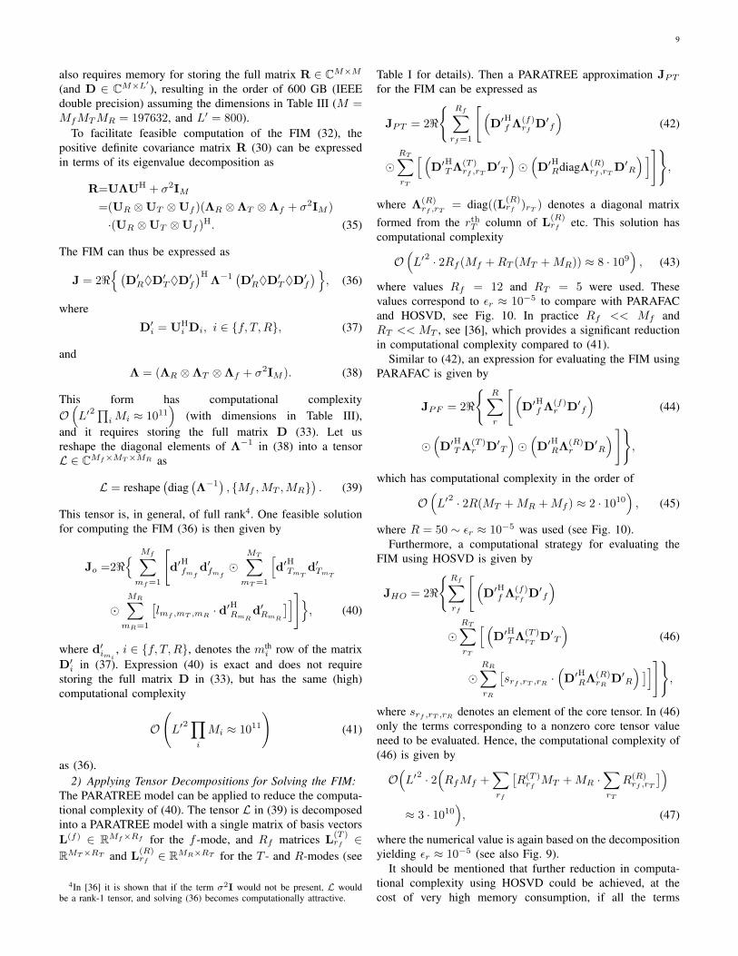
As discussed in Section IV-B, the PARATREE approxi-mation can be used to reduce computational complexity ofcalculating the FIM in certain applications. Fig. 9 illustratesthe performance of different tensor decompositions in termsof computational complexity while computing the Fisherinformation matrix (excluding the complexity of comput-ing the tensor decomposition). The complexities are givenby the equations (41) (exact), (43) (PARATREE), and (45)(PARAFAC), and are normalized by the complexity of theexact solution (41). The complexities are averaged by approx-imating 1500 realizations of the tensor L (39) with differentrelative approximation errors (20). Additionally, the influenceof varying the dimension order is studied for PARATREE.It can be seen that the complexity is clearly lowest whileapplying PARATREE with the largest dimension decomposedfirst. The comparison results for PARAFAC-ALS are obtainedusing random initialization of the factors, and for two Rvalues (R = 10, 50) only. For higher rank approximations(R = 100, 200), the algorithm failed to converge in areasonable time. The considered HOSVD strategy (46) hasthe highest complexity in this task, and the complexity caneven grow higher than that of the exact solution.
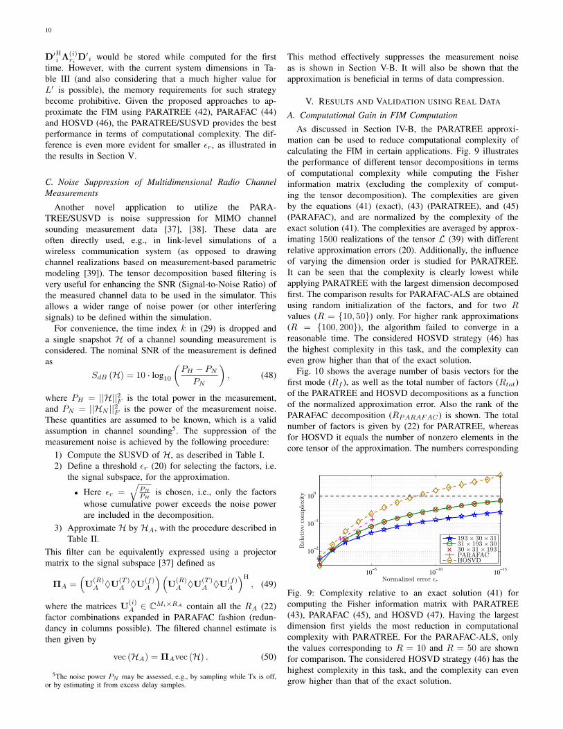
Fig. 10 shows the average number of basis vectors for thefirst mode (Rf ), as well as the total number of factors (Rtot)of the PARATREE and HOSVD decompositions as a functionof the normalized approximation error. Also the rank of thePARAFAC decomposition (RPARAFAC) is shown. The totalnumber of factors is given by (22) for PARATREE, whereasfor HOSVD it equals the number of nonzero elements in thecore tensor of the approximation. The numbers corresponding
Fig. 9: Complexity relative to an exact solution (41) forcomputing the Fisher information matrix with PARATREE(43), PARAFAC (45), and HOSVD (47). Having the largestdimension first yields the most reduction in computationalcomplexity with PARATREE. For the PARAFAC-ALS, onlythe values corresponding to R = 10 and R = 50 are shownfor comparison. The considered HOSVD strategy (46) has thehighest complexity in this task, and the complexity can evengrow higher than that of the exact solution.
11
to εr = 10−5 were used in the complexity evaluation inSection IV-B ((43), (45), and (47)).
B. Filtering of MIMO Channel Sounding Measurements
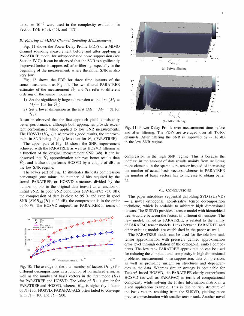
Fig. 11 shows the Power-Delay Profile (PDP) of a MIMOchannel sounding measurement before and after applying aPARATREE model for subspace-based noise suppression (seeSection IV-C). It can be observed that the SNR is significantlyimproved (noise is suppressed) after filtering, especially in thebeginning of the measurement, where the initial SNR is alsovery low.
Fig. 12 shows the PDP for three time instants of thesame measurement as Fig. 11. The two filtered PARATREEestimates of the measurement H1 and H2 refer to differentordering of the tensor modes as:
1) Set the significantly largest dimension as the first (M1 =Mf = 193 for H1)
2) Set a lower dimension as the first (M1 = MT = 31 forH2).
It can be observed that the first approach yields consistentlybetter performance, although both approaches provide excel-lent performance while applied to low SNR measurements.The HOSVD (HHO) also provides good results, the improve-ment in SNR being slightly less than for H1 (PARATREE).
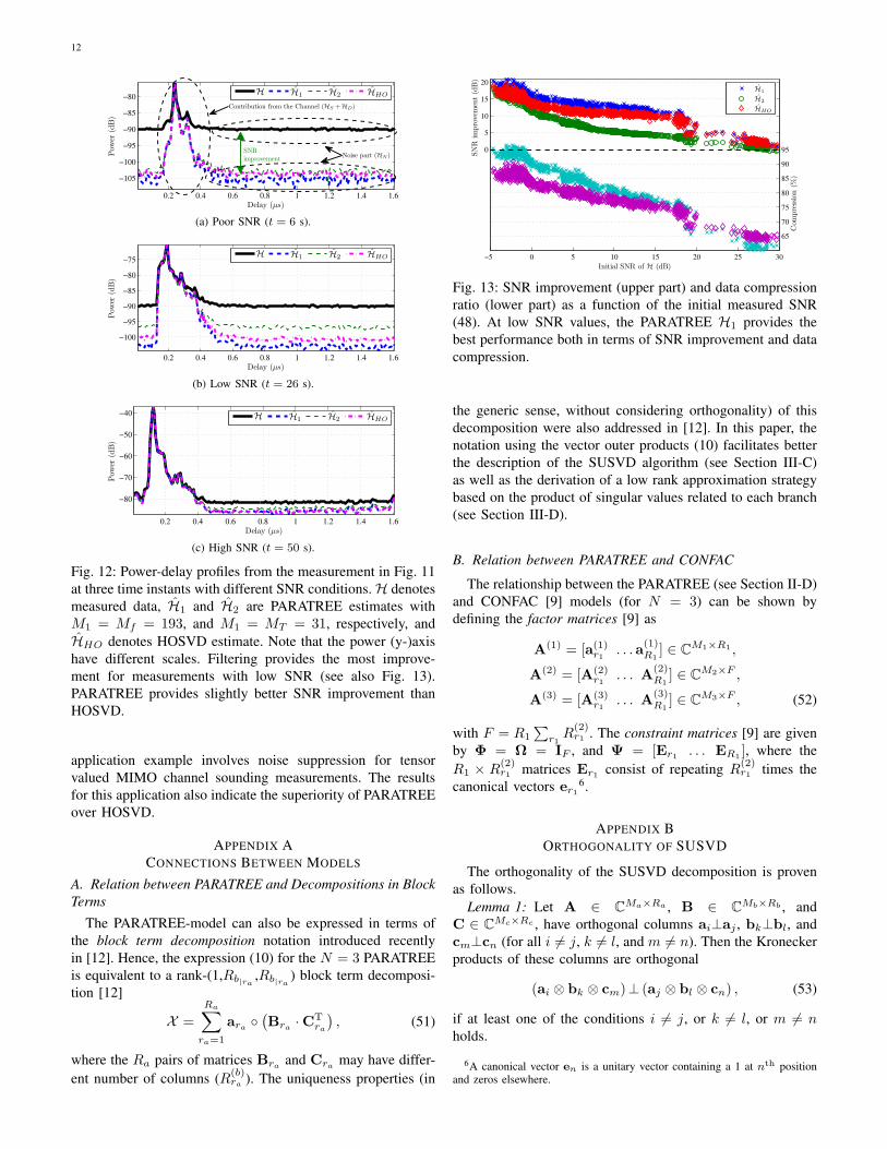
The upper part of Fig. 13 shows the SNR improvementachieved with the PARATREE as well as HOSVD filtering asa function of the original measurement SNR (48). It can beobserved that H1 approximation achieves better results thanH2, and it also outperforms HOSVD by a couple of dBs inthe low SNR regime.
The lower part of Fig. 13 illustrates the data compressionpercentage (one minus the number of bits required by thestored PARATREE or HOSVD structures divided by thenumber of bits in the original data tensor) as a function ofinitial SNR. In poor SNR conditions (SNRdB(H) < 0 dB),the compression of data is close to 95 % and even in goodSNR (SNRdB(H) > 25 dB), the compression is in the orderof 60 %. The HOSVD outperforms PARATREE in terms of
10−15
10−10
10−5
101
102
103
104
Normalized error ǫr
Num
ber
offa
ctor
s
RtotRf
RPARAFACPARATREEHOSVD
Fig. 10: The average of the total number of factors (Rtot) fordifferent decompositions as a function of normalized error, aswell as the number of basis vectors in the first mode (Rf )for PARATREE and HOSVD. The value of Rf is similar forPARATREE and HOSVD, whereas Rtot is higher (by a factorof RR) for HOSVD. PARAFAC-ALS often failed to convergewith R = 100 and R = 200.
(a) Before filtering.
(b) After filtering.
Fig. 11: Power-Delay Profile over measurement time beforeand after filtering. The PDPs are averaged over all Tx-Rxchannels. After filtering the SNR is improved by ∼ 15 dBin the low SNR regime.
compression in the high SNR regime. This is because theincrease in the amount of data results mainly from includingmore elements in the sparse core tensor instead of increasingthe number of actual basis vectors, whereas in PARATREEthe number of basis vectors has to increase to obtain betterfit.
VI. CONCLUSIONS
This paper introduces Sequential Unfolding SVD (SUSVD)— a novel orthogonal, non-iterative tensor decompositiontechnique, which is scalable to arbitrary high dimensionaltensors. The SUSVD provides a tensor model with hierarchicaltree structure between the factors in different dimensions. Thenew model, named as PARATREE, is related to the familyof PARAFAC tensor models. Links between PARATREE andother existing models are established in the paper as well.
The PARATREE model can be used for flexible low ranktensor approximation with precisely defined approximationerror level through deflation of the orthogonal rank-1 compo-nents. The low rank PARATREE approximation can be usedfor reducing the computational complexity in high dimensionalproblems, measurement noise suppression, data compression,as well as providing insight on structures and dependen-cies in the data. Whereas similar strategy is obtainable forTucker3 based HOSVD, the PARATREE clearly outperformsHOSVD (as well as PARAFAC) in terms of computationalcomplexity while solving the Fisher Information matrix in agiven application example. This is due to rich structure ofthe basis vectors resulting from the SUSVD, yielding moreprecise approximation with smaller tensor rank. Another novel
12
0.2 0.4 0.6 0.8 1 1.2 1.4 1.6
−105
−100
−95
−90
−85
−80
Delay (µs)
Pow
er(d
B)
H H1 H2 HHO
SNRimprovement
Contribution from the Channel (HS +HD)
Noise part (HN )
(a) Poor SNR (t = 6 s).
0.2 0.4 0.6 0.8 1 1.2 1.4 1.6
−100
−95
−90
−85
−80
−75
Delay (µs)
Pow
er(d
B)
H H1 H2 HHO
(b) Low SNR (t = 26 s).
0.2 0.4 0.6 0.8 1 1.2 1.4 1.6
−80
−70
−60
−50
−40
Delay (µs)
Pow
er(d
B)
H H1 H2 HHO
(c) High SNR (t = 50 s).
Fig. 12: Power-delay profiles from the measurement in Fig. 11at three time instants with different SNR conditions.H denotesmeasured data, H1 and H2 are PARATREE estimates withM1 = Mf = 193, and M1 = MT = 31, respectively, andHHO denotes HOSVD estimate. Note that the power (y-)axishave different scales. Filtering provides the most improve-ment for measurements with low SNR (see also Fig. 13).PARATREE provides slightly better SNR improvement thanHOSVD.
application example involves noise suppression for tensorvalued MIMO channel sounding measurements. The resultsfor this application also indicate the superiority of PARATREEover HOSVD.
APPENDIX ACONNECTIONS BETWEEN MODELS
A. Relation between PARATREE and Decompositions in BlockTerms
The PARATREE-model can also be expressed in terms ofthe block term decomposition notation introduced recentlyin [12]. Hence, the expression (10) for the N = 3 PARATREEis equivalent to a rank-(1,Rb|ra
,Rb|ra) block term decomposi-
tion [12]
X =Ra∑
ra=1
ara(Bra·CT
ra
), (51)
where the Ra pairs of matrices Braand Cra
may have differ-ent number of columns (R(b)
ra ). The uniqueness properties (in
0
5
10
15
20
Initial SNR of H (dB)
SNR
impr
ovem
ent
(dB
)
−5 0 5 10 15 20 25 30
65
70
75
80
85
90
95
Com
pres
sion
(%)
H1
H2
HHO
Fig. 13: SNR improvement (upper part) and data compressionratio (lower part) as a function of the initial measured SNR(48). At low SNR values, the PARATREE H1 provides thebest performance both in terms of SNR improvement and datacompression.
the generic sense, without considering orthogonality) of thisdecomposition were also addressed in [12]. In this paper, thenotation using the vector outer products (10) facilitates betterthe description of the SUSVD algorithm (see Section III-C)as well as the derivation of a low rank approximation strategybased on the product of singular values related to each branch(see Section III-D).
B. Relation between PARATREE and CONFAC
The relationship between the PARATREE (see Section II-D)and CONFAC [9] models (for N = 3) can be shown bydefining the factor matrices [9] as
A(1) = [a(1)r1
. . .a(1)R1
] ∈ CM1×R1 ,
A(2) = [A(2)r1
. . . A(2)R1
] ∈ CM2×F ,
A(3) = [A(3)r1
. . . A(3)R1
] ∈ CM3×F , (52)
with F = R1
∑r1R
(2)r1 . The constraint matrices [9] are given
by Φ = Ω = IF , and Ψ = [Er1 . . . ER1 ], where theR1 × R(2)
r1 matrices Er1 consist of repeating R(2)r1 times the
canonical vectors er16.
APPENDIX BORTHOGONALITY OF SUSVD
The orthogonality of the SUSVD decomposition is provenas follows.
Lemma 1: Let A ∈ CMa×Ra , B ∈ CMb×Rb , andC ∈ CMc×Rc , have orthogonal columns ai⊥aj , bk⊥bl, andcm⊥cn (for all i 6= j, k 6= l, and m 6= n). Then the Kroneckerproducts of these columns are orthogonal
(ai ⊗ bk ⊗ cm)⊥ (aj ⊗ bl ⊗ cn) , (53)
if at least one of the conditions i 6= j, or k 6= l, or m 6= nholds.
6A canonical vector en is a unitary vector containing a 1 at nth positionand zeros elsewhere.
13
Proof: The proof is given by evaluating the inner product
(ai ⊗ bk ⊗ cm)H (aj ⊗ bl ⊗ cn)
=(aH
i ⊗ [bk ⊗ cm]H)
(aj ⊗ [bl ⊗ cn])
=(aH
i aj
)⊗([bk ⊗ cm]H ⊗ [bl ⊗ cn]
)=(aH
i aj
)⊗(bH
k bl
)⊗(cH
mcn
). (54)
The expression (54) is zero if any of the three terms in theKronecker product of the last row are zero. Hence, the vectors(ai ⊗ bk ⊗ cm) and (aj ⊗ bl ⊗ cn) are always orthogonal((54) is nonzero), except when i = j, and k = l, and m = n.
Now let us consider the outer product form of PARATREEfor N = 3
X=R1∑
r1=1
σ(1)r1· u(1)
r1
R2∑r2=1
(σ(2)
r1,r2· u(2)
r1,r2 u(3)
r1,r2
)(55)
=R1∑
r1=1
R2∑r2=1
(σ(1)
r1σ(2)
r1,r2· u(1)
r1 u(2)
r1,r2 u(3)
r1,r2
).
The orthogonality of the conventional 2-D SVD decompositionwithin the SUSVD computation yields(
Given the above conditions (56) along with Lemma 1, yields,for the three-way example in (55),(
u(1)r1⊗ u(2)
r1,r2⊗ u(3)
r1,r2
)H (u(1)
q1⊗ u(2)
q1,q2⊗ u(3)
q1,q2
)= 0,
(57)for all values except if r1, r2 = q1, q2. The summationindexes in (55) result only in values for which the basisvectors are orthogonal in at least one of the dimensions. Hence,all the complete Kronecker (or outer) product terms in thedecomposition are orthogonal. The proof applies eqivalentlyto higher order tensors.
ACKNOWLEDGMENT
The authors would like to acknowledge the effort of Veli-Matti Kolmonen, Jukka Koivunen, Katsuyuki Haneda, PeterAlmers, and Mario Costa who were involved in performingthe channel sounding measurements used in this paper inSeptember 2007 at Espoo, Finland.
REFERENCES
[1] R. A. Harshman, “Foundations of the PARAFAC procedure: Modelsand conditions for an ‘explanatory’ multi-modal factor analysis,” UCLAworking papers in phonetics, vol. 16, 1970.
[2] L. R. Tucker, “Some mathematical notes on three-mode factor analysis,”Psychometrika, vol. 36, pp. 279–311, 1966.
[3] J. B. Kruskal, “Three-way arrays: rank uniqueness of trilinear decompo-sitions, with application to arithmetic complexity and statistics,” LinearAlgebra Appl., vol. 18, pp. 95–138, 1977.
[4] J. D. Carroll and J. J. Chang, “Analysis of individual differences inmultidimensional scaling via an N-way generalization of ‘Eckart-Young’decomposition,” Psychometrika, vol. 35, pp. 283–319, 1970.
[5] J. D. Carroll, S. Pruzansky, and J. Kruskal, “Candelinc: A generalapproach to multidimensional analysis of many-way arrays with linearconstraints on parameters,” Psychometrika, vol. 45, no. 1, pp. 3–24, Mar.1980.
[6] N. K. M. Faber, R. Bro, and P. K. Hopke, “Recent developments inCANDECOMP/PARAFAC algorithms: a critical review,” Chemometricsand Intelligent Laboratory Systems, vol. 65, no. 1, pp. 119–137, Jan.2003.
[7] A. L. F. de Almeida, G. Favier, J. C. M. Mota, and R. L. de Lacerda,“Estimation of frequency-selective block-fading MIMO channels usingPARAFAC modeling and alternating least squares,” in The 40th AsilomarConference on Signals, Systems and Computers, Pacific Grove, CA,Oct.–Nov. 2006, pp. 1630–1634.
[8] N. Sidiropoulos, R. Bro, and G. Giannakis, “Parallel factor analysisin sensor array processing,” IEEE Transactions on Signal Processing,vol. 48, no. 8, pp. 2377–2388, Aug. 2000.
[9] A. de Almeida, G. Favier, and J. Mota, “A constrained factor decompo-sition with application to MIMO antenna systems,” IEEE Transactionson Signal Processing, vol. 56, no. 6, pp. 2429–2442, Jun. 2008.
[10] L. De Lathauwer, B. De Moor, and J. Vandewalle, “A multilinearsingular value decomposition,” SIAM J. Matrix Anal. Appl., vol. 21,no. 4, pp. 1253–1278, 2000.
[11] M. Haardt, F. Roemer, and G. Del Galdo, “Higher-order SVD-basedsubspace estimation to improve the parameter estimation accuracy inmultidimensional harmonic retrieval problems,” IEEE Transactions onSignal Processing, vol. 56, no. 7, pp. 3198–3213, Jul. 2008.
[12] L. De Lathauwer, “Decompositions of a higher-order tensor in blockterms — Part II: Definitions and uniqueness,” SIAM J. Matrix Anal.Appl., vol. 30, no. 3, pp. 1033–1066, 2008. [Online]. Available:http://publi-etis.ensea.fr/2008/De 08f
[13] Mathworks. Matlab. [Online]. Available: http://www.mathworks.com[14] T. G. Kolda and B. W. Bader, “Tensor decompositions and applications,”
SIAM Review, vol. 51, no. 3, Sept. 2009, to appear.[15] A. Smilde, R. Bro, and P. Geladi, Multiway Analysis with Applications
in the Chemical Sciences. Chichester, England: John Wiley and Sons,Ltd, 2004, 381 p.
[16] N. D. Sidiropoulos and R. Bro, “On the uniqueness of multilineardecomposition of N -way arrays,” Journal of Chemometrics, vol. 14,no. 3, pp. 229–239, May 2000.
[17] A. Stegeman, J. Berge, and L. Lathauwer, “Sufficient conditions foruniqueness in candecomp/parafac and indscal with random componentmatrices,” Psychometrika, vol. 71, no. 2, pp. 219–229, Jun. 2006.
[18] L. De Lathauwer, B. De Moor, and J. Vandewalle, “On the best rank-1and rank-(r1, r2, ..., rn) approximation of higher-order tensors,” SIAMJournal on Matrix Analysis and Applications, vol. 21, no. 4, pp. 1324–1342, 2000. [Online]. Available: http://link.aip.org/link/?SML/21/1324/1
[19] P. Comon and J. ten Berge, “Generic and typical ranks of three-wayarrays,” in IEEE International Conference on Acoustics, Speech andSignal Processing (ICASSP 2008), Las Vegas, NV, Apr. 2008, pp. 3313–3316.
[20] T. G. Kolda, “Multilinear operators for higher-order decompositions,”Sandia National Laboratories, Albuquerque, NM and Livermore, CA,Technical Report SAND2006-2081, Apr. 2006. [Online]. Available:http://csmr.ca.sandia.gov/˜tgkolda/pubs/
[21] R. Bro and H. A. L. Kiers, “A new efficient method for determining thenumber of components in PARAFAC models,” Journal of Chemometrics,vol. 17, no. 5, pp. 274–286, 2003.
[22] E. Kofidis and P. A. Regalia, “On the best rank-1 approximationof higher-order supersymmetric tensors,” SIAM J. Matrix Anal. Appl,vol. 23, pp. 863–884, 2002.
[23] T. G. Kolda, “A counterexample to the possibility of an extension ofthe Eckart-Young low-rank approximation theorem for the orthogonalrank tensor decomposition,” SIAM Journal on Matrix Analysis andApplications, vol. 24, no. 3, pp. 762–767, January 2003.
[24] R. Bro, R. A. Harshman, and N. D. Sidiropoulos, “Modeling multi-way data with linearly dependent loadings,” Dept. of Dairy and FoodScience, The Royal Veterinary and Agricultural University, Copenhagen,Denmark, Technical Report 2005-176, 2005.
[25] L. De Lathauwer, B. De Moor, and J. Vandewalle, “Computation of thecanonical decomposition by means of a simultaneous generalized Schurdecompositition,” SIAM J. Matrix Anal. Appl., vol. 26, no. 2, pp. 295–327, 2004. [Online]. Available: http://publi-etis.ensea.fr/2004/DDV04
[26] P. Kroonenberg and J. De Leeuw, “Principal component analysis ofthree-mode data by means of alternating least squares algorithms,”Psychometrika, vol. 45, no. 1, pp. 69–97, Mar. 1980.
14
[27] G. Tomasi and R. Bro, “A comparison of algorithms for fitting thePARAFAC model,” Computational Statistics & Data Analysis, vol. 50,no. 7, pp. 1700–1734, Apr. 2006.
[28] P. K. Hopke, P. Paatero, H. Jia, R. T. Ross, and R. A. Harshman,“Three-way (PARAFAC) factor analysis: examination and comparisonof alternative computational methods as applied to ill-conditioned data,”Chemometrics and Intelligent Laboratory Systems, vol. 43, pp. 25–42,Sept. 1998.
[29] A. Richter, “Estimation of radio channel parameters: Models andalgorithms,” Ph. D. dissertation, Technischen Universitat Ilmenau,Germany, May 2005, ISBN 3-938843-02-0. [Online]. Available:www.db-thueringen.de
[30] V.-M. Kolmonen, J. Kivinen, L. Vuokko, and P. Vainikainen, “5.3-GHzMIMO radio channel sounder,” IEEE Transactions on Instrumentationand Measurement, vol. 55, no. 4, pp. 1263–1269, Aug. 2006.
[31] J. Koivunen, P. Almers, V.-M. Kolmonen, J. Salmi, A. Richter, F. Tufves-son, P. Suvikunnas, A. Molisch, and P. Vainikanen, “Dynamic multi-link indoor MIMO measurements at 5.3 GHz,” in The 2nd EuropeanConference on Antennas and Propagation (EuCAP 2007), Edinburgh,UK, Nov. 2007, pp. 1–6.
[32] J. Salmi, A. Richter, and V. Koivunen, “Detection and tracking ofMIMO propagation path parameters using state-space approach,” IEEETransactions on Signal Processing, vol. 57, no. 4, pp. 1538–1550, April2009.
[33] ——, “Enhanced tracking of radio propagation path parameters usingstate-space modeling,” in The 14th European Signal Processing Confer-ence (EUSIPCO 2006), Florence, Italy, Sept. 4–8 2006.
[34] M. Landmann, “Limitations of experimental channel characterization,”Ph. D. dissertation, Technischen Universitat Ilmenau, Ilmenau, Germany,Mar. 2008. [Online]. Available: http://www.db-thueringen.de
[35] A. Richter, J. Salmi, and V. Koivunen, “ML estimation of covariancematrix for tensor valued signals in noise,” in IEEE International Confer-ence on Acoustics, Speech, and Signal Processing (ICASSP 2008), LasVegas, USA, Mar. 31–Apr. 4 2008, pp. 2349–2352.
[36] J. Salmi, A. Richter, and V. Koivunen, “Tracking of MIMO propagationparameters under spatio-temporal scattering model,” in The 41st Asilo-mar Conference on Signals, Systems, and Computers, Pacific Grove, CA,Nov. 2007, pp. 666–670.
[37] A. Richter, J. Salmi, and V. Koivunen, “Tensor decomposition of MIMOchannel sounding measurements and its applications,” in URSI GeneralAssembly, Chicago, USA, Aug. 7–16 2008.
[38] J. Salmi, A. Richter, and V. Koivunen, “Sequential unfolding SVDfor low rank orthogonal tensor approximation,” in The 42nd AsilomarConference on Signals, Systems, and Computers, Pacific Grove, CA,Oct. 2008, pp. 1713–1717.
[39] U. Trautwein, C. Schneider, and R. Thoma, “Measurement-based per-formance evaluation of advanced MIMO transceiver designs,” EURASIPJournal on Applied Signal Processing, vol. 2005, no. 1, pp. 1712–1724,2005.
Jussi Salmi (S’05) was born in Finland in 1981. Hereceived his M.Sc. degree with honors from HelsinkiUniversity of Technology, Dept. of Electrical andCommunications Engineering, Espoo, Finland, in2005, and is currently finalizing his Ph.D. degree.From 2004 to 2005, he worked as a ResearchAssistant at Radio Laboratory, Helsinki Universityof Technology. Since 2005 he has held a Researcherposition at Dept. of Signal Processing and Acoustics,Helsinki University of Technology. Since 2007 hehas been a member of Graduate School in Elec-
tronics, Telecommunications and Automation (GETA). His current researchinterests include measurement based MIMO channel modeling, parameterestimation, analysis of interference limited multiuser MIMO measurementsas well as tensor modeling and decomposition techniques. He has authoreda paper receiving the Best Student Paper Award in (EUSIPCO’06), and co-authored a paper receiving the Best Paper Award in Propagation (EuCAP’06).
Andreas Richter (M04, SM08) received the Dipl.-Ing. (M.Sc.) degree in electrical engineering and theDr.-Ing. (Ph.D.) degree (summa cum laude) fromTechnische Universitat Ilmenau, Ilmenau, Germany,in 1995 and 2005, respectively. From 1995 to 2004,he worked as a Research Assistant at ElectronicMeasurement Laboratory of Technische UniversitatIlmenau. From July to October 2001, he was a GuestResearcher at NTT DoCoMo’s, Wireless Laborato-ries, Yokosuka, Japan. From 2004 to 2008, he hasbeen working as a Senior Research Fellow in the
Statistical Signal Processing Laboratory at Helsinki University of Technology,Finland. Since August 2008, he is Principal Member of Research Staff atNokia Research Center, Helsinki. His research interests are in the fields ofdigital communication, sensor-array-, and statistical signal processing. Hehas published more than 80 peer-reviewed papers in international scientificconferences and journals. Dr. Richter has co-authored or authored of fivepapers receiving a Best Paper Award (EPMCC01, ISAP04, PIMRC05, EU-SIPCO06, and EuCAP06). In 2005, he received the Siemens CommunicationsAcademic Award. He and his former colleagues at Technische UniversitatIlmenau received the Thuringian Research Award for Applied Research in2007 for their work on MIMO channel sounding.
Visa Koivunen (S’87-M’93-SM’98) received hisD.Sc. (Tech) degree with honors from the Univer-sity of Oulu, Dept. of Electrical Engineering. Hereceived the primus doctor (best graduate) awardamong the doctoral graduates in years 1989-1994.From 1992 to 1995 he was a visiting researcher atthe University of Pennsylvania, Philadelphia, USA.From 1997 to 1999 he was an Associate Professorat the Signal Processing Labroratory, Tampere Uni-versity of Technology. Since 1999 he has been aProfessor of Signal Processing at Helsinki University
of Technology (HUT), Finland. He is one of the Principal Investigatorsin SMARAD (Smart Radios and Wireless Systems) Center of Excellencein Radio and Communications Engineering nominated by the Academyof Finland. He has been also adjunct full professor at the University ofPennsylvania, Philadelphia, USA. During his sabbatical leave in 2006–2007he was Visiting Fellow at Nokia Research Center as well as at PrincetonUniversity.
Dr. Koivunen’s research interest include statistical, communications andsensor array signal processing. He has published more than 280 papers ininternational scientific conferences and journals. He co-authored the papersreceiving the best paper award in IEEE PIMRC 2005, EUSIPCO 2006 andEuCAP 2006. He has been awarded the IEEE Signal Processing Societybest paper award for the year 2007 (co-authored with J. Eriksson). Heserved as an associate editor for IEEE Signal Processing Letters. He is amember of the editorial board for the Signal Processing journal and Journalof Wireless Communication and Networking. He is also a member of the IEEESignal Processing for Communication and Networking Technical Committee(SPCOM-TC) and Sensor Array and Multichannel Technical Committee(SAM-TC). He was the general chair of the IEEE SPAWC (Signal ProcessingAdvances in Wireless Communication) 2007 conference in Helsinki, June2007.