Just starting out: Learning and equilibrium in a new market * Ulrich Doraszelski University of Pennsylvania, CEPR, and NBER Gregory Lewis Microsoft Research and NBER Ariel Pakes Harvard University and NBER September 26, 2017 Abstract We document the evolution of the new market for frequency response within the UK electricity system over a six-year period. Firms competed in price while facing considerable initial uncertainty about demand and rival behavior. We show that over time prices stabilized, converging to a rest point that is consistent with equilibrium play. We draw on models of fictitious play and adaptive learning to analyze how this convergence occurs and show that these models predict behavior better than an equilibrium model prior to convergence. * We thank four referees and the editor for helpful comments. We are grateful to Paul Auckland and Graham Hathaway of National Grid and Ian Foy of Drax Power for useful conversations about this project. We have benefited from discussions with Joseph Cullen, Glenn Ellison, Ignacio Esponda, Drew Fudenberg, Mar Reguant and Frank Wolak, and from the comments of seminar participants at Boston College, Cornell, Duke, Harvard/MIT, Kellogg, Princeton, Washington University and the NBER Productivity Lunch and IO Program Meeting. Rebecca Diamond, Duncan Gilchrist, Matthew Hlavacek, Tim O’Connor, Daniel Pollmann, Sean Smith, Amanda Starc, and Wei Sun have all provided excellent research assistance.
Transcript
Just starting out: Learning and equilibrium in a new
market∗
Ulrich Doraszelski
University of Pennsylvania, CEPR, and NBER
Gregory Lewis
Microsoft Research and NBER
Ariel Pakes
Harvard University and NBER
September 26, 2017
Abstract
We document the evolution of the new market for frequency response within the
UK electricity system over a six-year period. Firms competed in price while facing
considerable initial uncertainty about demand and rival behavior. We show that over
time prices stabilized, converging to a rest point that is consistent with equilibrium
play. We draw on models of fictitious play and adaptive learning to analyze how
this convergence occurs and show that these models predict behavior better than an
equilibrium model prior to convergence.
∗We thank four referees and the editor for helpful comments. We are grateful to Paul Auckland andGraham Hathaway of National Grid and Ian Foy of Drax Power for useful conversations about this project.We have benefited from discussions with Joseph Cullen, Glenn Ellison, Ignacio Esponda, Drew Fudenberg,Mar Reguant and Frank Wolak, and from the comments of seminar participants at Boston College, Cornell,Duke, Harvard/MIT, Kellogg, Princeton, Washington University and the NBER Productivity Lunch andIO Program Meeting. Rebecca Diamond, Duncan Gilchrist, Matthew Hlavacek, Tim O’Connor, DanielPollmann, Sean Smith, Amanda Starc, and Wei Sun have all provided excellent research assistance.
1 Introduction
What do competing agents or firms do when their environment changes? Answering this
question is necessary for making predictions about market evolution following policy changes
or changes to market institutions. The approach to analyzing changes used in empirical
work is typically based on computing counterfactual equilibria. However, convergence to
equilibrium after a perturbation may not be swift or indeed certain, and the adjustment
mechanism may well be integral in determining which among alternative possible equilibria
the market converges to. Understanding how firms adjust and the ensuing learning process
is thus central to the analysis of environmental changes.
This paper offers a case study of a newly deregulated market, the frequency response (FR)
market in the UK. Initially, firms faced tremendous uncertainty both about the determinants
of demand and about what their rivals would do. Following Brandenburger (1996), we refer
to a firm’s uncertainty about the behavior of its rivals as strategic uncertainty.1 We explore
how demand and strategic uncertainty manifest themselves in the behavior of firms from
“day one,” tracing their behavior over the next six years.
Broadly speaking, FR is a product required by the system operator to keep the electricity
system running smoothly. Historically, electricity generating firms had been obligated to
provide FR to the system operator at a fixed price. Deregulation created a market in which
firms are allowed to bid for providing FR, thus setting the stage for price competition. An
attractive feature of this market is that the demand for FR and the set of market participants
were, at least in the first three and a half years, relatively stable, so that changes in bids can
be plausibly attributed to learning rather than changes in the environment.
The first part of the paper documents bidding behavior over time. We distinguish three
phases in the evolution of the FR market. The early phase of the FR market is characterized
by heterogeneous bidding behavior and frequent and sizeable adjustments of bids. Some firms
appear to experiment with their bids. Other firms appear to “follow the leader.” Yet other
firms do not change their bids at all for many months. The price of FR exhibits a noticeable
upward trend during the early phase that culminates in a “price bubble.” During the middle
phase of the FR market, this trend reverses itself. Competition between firms drives the
1Brandenburger (1996) draws a distinction between strategic uncertainty, i.e., uncertainty about theactions and beliefs of other players, and structural uncertainty, i.e., uncertainty about the primitives of thegame.
1
highest bids down, leading to a dramatic reduction in the range of bids. Adjustments of bids
are less frequent and smaller than in the early phase. By the time the FR market enters
its late phase, it appears to have reached a “rest point.” This rest point is consistent with
a complete information Nash equilibrium, and we show that thereafter bids stay close to
their equilibrium levels despite periodically occurring smaller changes in the environment.
The industrial organization literature routinely assumes that equilibrium reasserts itself, so
finding that it does in a particular example is reassuring (and to the best of our knowledge
ours is the first paper to empirically analyze the convergence process). On the other hand,
the FR market can only be considered to have converged to a rest point after three and a
half to four years of monthly strategic interaction.
The second part of the paper analyzes in more detail how this convergence occurs through
the “lens” of alternative learning models. To do so, we first estimate the demand and cost
primitives under a relatively weak rationality assumption that we view as appropriate for
the late phase of the FR market. This enables us to estimate profits for any vector of
bids. Assuming actual bids are determined by perceptions of likely profits, we can then
analyze how the realizations of its rivals’ bids and demand impact a firm’s perceptions of
the profitability of alternative strategies. To structure our analysis of strategic uncertainty
we use fictitious play models in which firms form their beliefs based on past observed rival
behavior (Brown 1951). To structure our analysis of firms’ perceptions about demand we use
adaptive learning models in which these perceptions are grounded in a statistical analysis of
the data they have available to them when they form their bids (Sargent 1993, Evans and
Honkapohja 2001, Evans and Honkapohja 2013). We judge alternative parameterizations
of our learning models by comparing both their “one-step-ahead” and “multi-period” bid
predictions to the actual bids.
The heterogeneous behavior and experimentation by some firms in the early phase of the FR
market is hard to rationalize with these models, so we focus our analysis of learning models
on the last two phases. During the middle phase of the FR market, the best-fitting models
are those in which firms more heavily weight recent rival behavior in forming beliefs about
their rivals’ bids and adaptively learn about the price elasticity of demand. In this phase
the predictions from the learning models are noticeably better than those from a complete
information Nash equilibrium where all agents know the demand parameters. Moreover, the
learning models make predictions which lead to what seems to be the “rest point” that we
observe in the last phase of the FR market. With some caveats that we point out below, our
2
work is therefore broadly supportive of these learning models — models that have previously
only been tested in lab experiments.
In contrast, during the late phase of the FR market the equilibrium model fits the data about
as well as the best learning models. Since there are a series of changes in the environment
that have been largely absent in the earlier phases, the performance of the equilibrium model
during this phase is notable. Of course, by the late phase firms had been able to acquire
quite a bit of information about rival behavior as well as demand.
Related literature. Our paper is closely related to a large body of work in micro, macro
and experimental economics. Going back to Cournot (1838), there has been work on the
theory of learning in normal-form and, more recently, extensive-form games. This literature
mainly aims to derive conditions on the underlying game under which the canonical models of
belief-based learning (including fictitious play) and reinforcement learning imply convergence
to equilibrium (Milgrom and Roberts 1991, Fudenberg and Kreps 1993, Borgers and Sarin
1997, Hart and Mas-Colell 2000). Belief-based learning starts with the premise that players
keep track of the history of play and form beliefs about what their rivals will do in the future
based on their past play. Reinforcement learning assumes that strategies are “reinforced”
by their past payoffs and that the propensity to choose a strategy depends in some way on
its stock of reinforcement.
Experimental economists have pushed this theoretical literature further by using lab exper-
iments to determine which learning models best describe how people actually learn (Erev
and Roth 1998). On the one hand, this has resulted in the development of more general
models such as experience-weighted attraction learning (Camerer and Ho 1999) and models
with sophisticated learners who try to influence how other players learn (Camerer, Ho and
Chong (2002); see also Mohlin, Ostling and Wang (2014) for an imitation dynamic consistent
with data from a Swedish gambling game). On the other hand, there is a growing consensus
that telling apart belief-based learning from reinforcement learning is difficult in practice
(Salmon 2001).
A second, distinct, theoretical literature considers behavior when agents have only partial
knowledge of the environment in which they operate. There is a long literature in applied
mathematics and statistics analyzing bandit problems, in which forward-looking agents trade
off “exploration” versus “exploitation” (Robbins 1952). Easley and Kiefer (1988) study under
what conditions optimizing agents learn the true parameters governing the data generating
3
process. Economists have also contributed to this literature by analyzing what happens when
multiple agents compete in a partially known environment, noting informational free-riding
incentives (Bolton and Harris 1999, Keller, Rady and Cripps 2005) and incentives to “signal
jam” (Riordan 1985, Mirman, Samuelson and Urbano 1993).
Macroeconomists largely think about learning in terms of expectation formation. The in-
fluential idea of adaptive learning (Sargent 1993, Evans and Honkapohja 2001, Evans and
Honkapohja 2013) posits that agents proceed like an econometrician and use the available
data to estimate a model of the economy and a rule for forming expectations. The cen-
tral question is whether the economy reaches a rational-expectations equilibrium. Large
shocks can have persistent effects through changing the agents’ “data sets” (Venkateswaran,
Veldkamp and Kozlowski 2015). There is also a corresponding experimental literature on
expectation formation (Fehr and Tyran 2008, Anufriev and Hommes 2012).
We combine models for beliefs about rival behavior with models for learning about the
underlying structural parameters and provide empirical evidence on how well they fit the
data. There is existing theoretical work on how firms learn about demand (Rothschild 1974,
Bergemann and Valimaki 1996, Bergemann and Valimaki 2006, Bernhardt and Taub 2015),
but little empirical work. What empirical work there is in the industrial organization and
marketing literatures is largely about how consumers experiment to learn their demand for
experience goods (Erdem and Keane 1996, Ackerberg 2003, Dickstein 2013) or how firms
learn about their cost (Griliches 1957, Porter 1995, Benkard 2000, Conley and Udry 2010,
Zhang 2010, Covert 2013, Newberry 2016).
There has been some empirical work assessing whether behavior in new markets converges to
some notion of equilibrium, but no structured analysis of how convergence occurs. Joskow,
Schmalensee and Bailey (1998) study the emissions rights market that was created by the
1990 Clean Air Act Amendments, concluding that the market “had become reasonably
efficient” (p. 669) within four years. Sweeting (2007) examines the electricity spot market
in England and Wales between 1995 and 2000, and finds evidence of tacit collusion between
the two largest generators. Hortacsu and Puller (2008) look at the electricity spot market in
Texas from 2001 to 2003, following a restructuring that introduced a uniform-price auction.
They find that firms with large stakes made bids that were close to optimal, while small
players deviated significantly. Luco, Hortacsu, Puller and Zhu (2017) further investigate the
impact of this heterogeneity in strategic ability on market efficiency.
4
Structure of paper. In Sections 2 and 3 we describe the FR market, our data, and offer
some descriptive evidence on how this market evolved over time. Section 4 outlines our
strategy for estimating the demand and cost primitives. In Section 5 we consider how well
different learning models fit the data, before concluding in Section 6. Additional derivations
and information on the construction of the data are contained in the data appendix. The
online appendix presents several robustness checks and extensions.
2 The FR market
The UK electricity market is a network of generators and distributors, connected by a trans-
mission grid. This grid is owned and operated by a company called National Grid plc (NG).
NG is responsible for the transmission of electricity from the generators to the distributors,
as well as the balancing of supply and demand in real time. Figure 1 summarizes the UK
electricity market.
The unit of exchange in this market is a given amount of power supplied for a half-hour (mea-
sured in megawatt hours (MWh)). About 98% of electricity is sold through bilateral forward
contracts between generators and distributors. These contracts can be formed months or
even years in advance. There are also shorter term contracts (both day ahead and day of)
which are often traded on power exchanges. One hour prior to the settlement period, both
generators and distributors must submit their contracted positions to NG, along with bids
and offers indicating the terms under which they are willing to be repositioned. NG then
acts to equate supply and demand over the settlement period by accepting bids and offers in
something akin to a multi-unit discriminatory auction. This process is called the balancing
mechanism (BM), and it accounts for the remaining 2% of electricity sales. The generators
bidding in the BM are called BM units. A power station typically consists of multiple BM
units, and multiple stations may be owned by the same firm. The BM units belonging to
the same station tend to be identical.
Frequency response. NG is obligated by government regulation to maintain a system
frequency within a one-percent band of 50Hz (Hertz, the number of cycles per second).
System frequency is determined in real time by imbalances between the supply and demand
of electricity. The higher demand is relative to supply, the lower the system frequency is,
5
Ratcliffe on Soar Kingsnorth
BM Unit Rats-2 Rats-1 Rats-3 Rats-4 Kino-1 Kino-2 Kino-3
Station Name
E.On Uk Party Name
Timeline
Gate closure: T – one hour Contractual positions
submitted
Forward contracts (98% of volume)
Balancing Mechanism (2%
of volume) APX spot
market
OTC forward contracts
Ofgem regulator
National Grid
Real-time
UK Electricity System
Mandatory Frequency Response
Simultaneously:
Balances supply and demand
Maintains system
frequency
Transmits
Distribution Companies
Consumers
Figure 1: Overview of the UK electricity market.
and vice versa. Imbalances occur due to shocks that cannot be corrected in advance through
the BM. To balance supply and demand in real time, NG instructs one or more BM units
into FR mode. Once in this mode, NG can rapidly adjust the electricity production of the
BM unit using so-called governor controls.
NG is required by government regulation to hold a certain amount of FR capacity at all
times.2 This response requirement is based on risk-response curves that assess the likelihood
2There are in fact three types of FR. Primary response is additional energy from a BM unit that isavailable ten seconds after an event and can be sustained for a further twenty seconds. Secondary responseis additional energy that is available within thirty seconds for up to thirty minutes. High response is areduction of energy within thirty seconds. These responses are technologically constrained and correspondto dilating the steam valve (primary), increasing the supply of fuel (secondary), and decreasing the supply offuel (high). For historical reasons, BM units are instructed into FR mode in the combinations primary-highand primary-secondary-high. To simplify the presentation and analysis, we aggregate the three types of FR(see the data appendix for details).
6
and magnitude of possible shocks given the total amount of electricity demanded. As the
total amount of electricity demanded evolves, NG instructs BM units in and out of FR mode
to satisfy its response requirement. To the best of our knowledge, the response requirement
remained unchanged over the sample period.3
FR services are thus a second product, distinct from electricity, that BM units can sell to
NG, and the FR market is distinct from the main market (comprised of the BM and bilateral
forward contracts). Providing FR is costly: a BM unit in FR mode incurs additional wear
and tear as it may have to make rapid, small adjustments to its electricity production in
response to supply and demand shocks. It also runs less efficiently, with a degraded heat
rate. The BM unit is compensated by NG by a holding payment and an energy response
payment. The holding payment is per unit of FR capacity and paid for the time that the
BM unit spends in FR mode, regardless of whether or not it actually makes adjustments
to its electricity production. We explain below in more detail how the holding payment is
calculated. The energy response payment compensates the BM unit for the adjustments
to its electricity production that NG calls for to maintain system frequency (when actually
needed).4 The energy response payment is considered by industry insiders to be a relatively
small source of profit, and is thus ignored in what follows.5
Deregulation. Our interest in FR stems from a change in the way the holding payment is
determined. This change occurred with the enactment of an amendment to the Connection
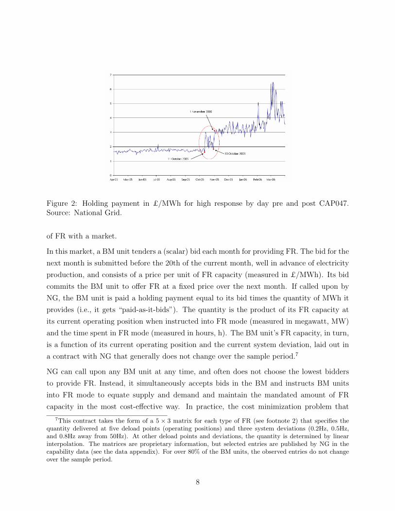
and Use of System Code called CAP047 and “went live” on November 1, 2005. Pre CAP047,
providing FR was mandatory, and the holding payment was at an administered price which
had been fairly constant over time (see Figure 2).6 CAP047 replaced the mandatory provision
3We have checked the publicly available minutes of all meetings of the Balancing Services Standing Group(comprising representatives of the generators and NG) and found no discussion of a change in the responserequirement.
4If the BM unit produces more energy than it was initially contracted to in the BM, NG pays it 125% ofthe current market price per additional unit of energy; if the BM unit produces less energy, it pays NG 75%of the current market price.
5FR services are paid for by NG, who in turn charges both generators and distribution companiesand ultimately consumers through the basic service charge, see https://www.ofgem.gov.uk/electricity/
transmission-networks/charging for additional details.6According to an OFGEM report (https://www.ofgem.gov.uk/publications-and-updates/
potential-income-adjusting-events-under-ngets-200506-system-operator-incentive-scheme)the volatility during the period from October 11 to October 30, 2005 was due to a dispatch error resultingfrom a new FR provider being dispatched on indicative contract prices, but settled at higher final contractprices, which had not been updated in NG’s dispatch file. Adjusting for this event, NG advised that theaverage holding payment price in October 2005 would have been £1.75/MWh.
7
Figure 2: Holding payment in £/MWh for high response by day pre and post CAP047.Source: National Grid.
of FR with a market.
In this market, a BM unit tenders a (scalar) bid each month for providing FR. The bid for the
next month is submitted before the 20th of the current month, well in advance of electricity
production, and consists of a price per unit of FR capacity (measured in £/MWh). Its bid
commits the BM unit to offer FR at a fixed price over the next month. If called upon by
NG, the BM unit is paid a holding payment equal to its bid times the quantity of MWh it
provides (i.e., it gets “paid-as-it-bids”). The quantity is the product of its FR capacity at
its current operating position when instructed into FR mode (measured in megawatt, MW)
and the time spent in FR mode (measured in hours, h). The BM unit’s FR capacity, in turn,
is a function of its current operating position and the current system deviation, laid out in
a contract with NG that generally does not change over the sample period.7
NG can call upon any BM unit at any time, and often does not choose the lowest bidders
to provide FR. Instead, it simultaneously accepts bids in the BM and instructs BM units
into FR mode to equate supply and demand and maintain the mandated amount of FR
capacity in the most cost-effective way. In practice, the cost minimization problem that
7This contract takes the form of a 5 × 3 matrix for each type of FR (see footnote 2) that specifies thequantity delivered at five deload points (operating positions) and three system deviations (0.2Hz, 0.5Hz,and 0.8Hz away from 50Hz). At other deload points and deviations, the quantity is determined by linearinterpolation. The matrices are proprietary information, but selected entries are published by NG in thecapability data (see the data appendix). For over 80% of the BM units, the observed entries do not changeover the sample period.
8
jointly governs the FR market and the BM is solved in real time by a proprietary linear
program running on a supercomputer. NG may not choose the lowest bids for at least three
reasons. First, BM units differ in the precision of their governor controls, and NG may prefer
to call upon more expensive but more precise BM units. The precision of a BM unit is thus
a source of product differentiation. Second, because the FR capacity of a BM unit depends
on its operating position, NG may prefer to call upon a BM unit operating in the middle of
its range, with plenty of FR capacity, rather than a BM unit operating at the extremes of its
range.8 Third, transmission constraints may affect the ability of some BM units to provide
FR and therefore make them ineligible.
The market for FR was proposed by RWE Npower Renewables Ltd., one of the largest firms
in the UK electricity market. This proposal was opposed by NG, who argued that since its
demand for FR is regulated and inelastic, firms would be able to exploit their market power
and the price of FR would rise. The government regulator dismissed these concerns and on
November 1, 2005 introduced CAP047. Figure 2 shows that NG had every reason to worry
about CAP047, as the holding payment doubled within the year.
From the pre-CAP047 period, firms had an understanding of the response requirement NG
is obligated to satisfy and the relative desirability of their BM units, as well as the cost of
providing FR. However, firms were uncertain about the demand for their FR services because
they did not know how their rivals would bid in the newly established market. In addition
to this strategic uncertainty, the firms faced demand uncertainty in that they did not know
how price sensitive NG was.
Our goal is to understand how firms learned to bid in the presence of this uncertainty, and
how this contributed to the evolution of the holding payment in Figure 2. The setup of
the FR market provides firms with ample opportunity to learn. NG regularly publishes the
submitted bids and the FR quantities it allocated to the various BM units. By the time a
firm prepares its bids for the next month, it knows its rivals’ bids up to and including the
current month and their FR quantities up to and including the previous month.
8Indeed, NG may first alter the operating position of the BM unit by taking over part of its obligationsin the BM before instructing the BM unit into FR mode. As a result, a BM unit does not have to withholdgenerating capacity from the main market in order to participate in the FR market. Our data shows thatBM units can — and do — contract out all of their capacity in the forward market while still activelyparticipating in the FR market. We thank Frank Wolak for pointing out to us that in many other countriesthe FR market is run separately from the BM. As a result, a BM unit has to withhold generating capacityto participate in the FR market. Because of the resulting opportunity cost, the holding payment is an orderof magnitude larger than in the UK.
9
Data. Our analysis focuses on the first six years of the operation of the FR market from
November 2005 to October 2011. We collected most of our data from two public sources.
Our data on the FR market comes from NG. For the post-CAP047 period we have the bids
submitted by each BM unit at a monthly level and the quantities provided of each type of
FR (in MWh, see footnote 2) by each BM unit at a daily level. The combination of bid and
quantity data allows us to calculate the holding payment received by each BM unit.
Our data on the BM comes from Elexon Ltd. Elexon is contracted by the government
regulator to manage measurement and financial settlement in the BM. For every BM unit
we have data on the bids and acceptances in the BM every half-hour. In combination with
data on the contracted position that the BM unit submits to NG one hour prior to the
settlement period, this allows us to assess the operating position of the BM unit.
Finally, we collected data on ownership and characteristics of power stations and fuel prices
from various sources. See the data appendix for further details on data sources as well as
sample and variable construction.
Market participants. There are 130 BM units grouped into 61 power stations owned by
29 firms. The FR market is mildly concentrated with a ten-firm-concentration ratio of 84%
and an HHI of 0.11 over the sample period.9 Table 1 summarizes revenue in the FR market
for the ten largest firms over the first six years of the market’s existence.
The largest firm, Drax, had over 20% of the FR market and earned about £100,000,000
over the sample period, or about £1,400,000 per month. Drax is a single-station firm,
while the next two largest firms, E.ON and RWE, are multi-station firms. Anecdotally,
Drax’s disproportionate share is attributable to having a relatively new plant, with accurate
governor controls, making it attractive for providing FR. The smallest firm, Seabank, still
makes around £200,000 per month. This suggests that the FR market was big enough that
firms may have been willing to devote time to actively managing their bidding strategy, at
least when the profitability of the market became apparent. Indeed, in 2006 Drax hired a
trader to specifically deal with the FR market.10 Within a year, Drax’s revenue from the
FR market increased more than threefold.
9For comparison, Sweeting (2007) reports an HHI in generation capacity of 0.1 for the England and Waleswholesale electricity market in 2001.
10Source: private discussion with Ian Foy, Head of Energy Management at Drax.
10
Table 1: Largest firms
Rank Firm name BM units Total Revenue Cumulativeowned revenue share (%) share (%)
Firms ranked by revenue in the FR market. BM units owned is the maximum number owned over the sampleperiod. Revenue is in inflation-adjusted millions of British pounds (base period is October 2011).
Supply and demand of FR. The demand for and supply of FR are relatively stable
over most of the sample period, although there are some changes to the market environment
towards the end of the sample. We argue this using a sequence of figures, each with dashed
vertical lines separating the three phases we distinguish below. Starting with the demand for
FR, the left panel of Figure 3 plots the monthly quantity of FR. Though this series is clearly
volatile, it is no more volatile at the beginning than at the end of the period we study (but,
as we show in Section 3, the bids are). The right panel of Figure 3 shows some evidence of
modest seasonality.
In addition to the mandatory frequency response (MFR) that is the focus of this paper,
NG uses proprietary long-term contracts with BM units to procure FR services. This is
known as firm frequency response (FFR). Figure 4 plots the monthly quantity of FFR and,
for comparison purposes, that of MFR (see also the left panel of Figure 3). The quantity
of FFR remains relatively stable over our sample period up until July 2010, when it almost
doubles and thereafter remains stable at the new level.
The vast majority of FFR is provided by pumped-storage BM units, who provide negligible
amounts of MFR. However, Drax — the largest firm in the MFR market — signed an FFR
contract from July to September 2007 and again from May to September 2010. This may
have been a short-lived attempt by NG to curtail the market power of Drax.
Figure 8: Quantity-weighted and unweighted absolute value of bid change conditional onchanging between month t and t− 1. Weights are based on month t− 1 and are zero if theBM unit’s bid did not change.
imentation became less prevalent over time.
Figure 11 shows the monthly bids of the eight largest power stations by revenue in the FR
market. The top left panel provides a more detailed look at the early phase. In line with the
wide range of bids documented in Figure 9 and the right panel of Figure 10, the levels and
trends of the bids are quite different across stations. Barking, Peterhead, and Seabank bid
very high early on — pricing themselves out of the market — and then drift back down into
contention. The remaining stations start low and then gradually ramp up. The big increase
in bids by Drax during late 2006 and early 2007 leads to the “price bubble” in Figure 6.
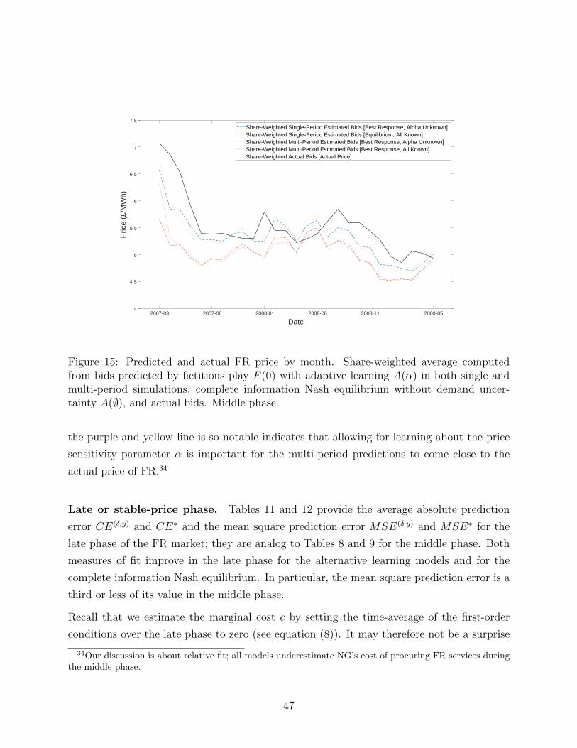
Middle or falling-price phase (March 2007 – May 2009). In the middle or falling-
price phase, firms change the bids of their BM units less often and by much smaller amounts
(in absolute value) than in the early phase. As Figures 7 and 8 illustrate on average the bids
of 3 out of 10 BM units change each month by around £1/MWh (conditional on changing).
Figure 9 shows that the range of bids is much narrower than in the early phase.
The top right panel of Figure 11 provides more detail. The “price bubble” bursts when
Seabank and Barking sharply decrease their bids and steal significant market share from
Drax. Drax follows Seabank and Barking down, and this inaugurates intense competition and
Figure 10: Quantity-weighted and unweighted variance in bids within a firm (left panel) andacross firms (right panel). The right panel shows quantity-weighted variance across firmsin the quantity-weighted mean firm bids and the unweighted variance across firms in theunweighted mean firm bids. Note the difference in the y-axes between panels.
bids of the different stations are noticeably closer to one another in this phase. By the time
the FR market has entered its late phase, it appears to have reached a “rest point” that is
periodically perturbed by small changes in the environment.
Summary. The early phase of the FR market is characterized by heterogeneous bidding
behavior and frequent and sizable adjustments of bids. During the middle and late phases,
bids grow closer and the frequency and size of adjustments to bids falls.
In the early or rising-price phase firms had no prior experience with bidding in the FR market.
Those firms who viewed the market as potentially profitable may have taken the opportunity
to experiment with their bids. This view is consistent with a comment by Ian Foy, head
of energy management at Drax, who stated: “The initial rush by market participants to
test the waters having no history to rely upon; to some extent it was guess work, follow the
price of others and try to figure out whether you have a competitive edge.” Different firms
pursued different strategies, with at least some firms responding to rivals’ experiments. As
a result, a model able to explain bidding behavior in the early phase is likely to have to
allow firms to consider the gains from alternative experiments in a competitive environment;
a task beyond the scope of this paper.
We view the middle or falling-price phase as a period of firms learning about how best to
maximize current profit. We thus treat the middle phase as dominated by firms bidding to
18
12345678910Weighted average bid (£/MWh)
2005
−10
2006
−01
2006
−04
2006
−07
2006
−10
2007
−01
Dat
e
Bar
king
Cot
tam
Con
nah’
s Q
uay
Dra
xE
ggbo
roug
hP
eter
head
Rat
sS
eaba
nk
12345678910Weighted average bid (£/MWh)
2007
−01
2007
−07
2008
−01
2008
−07
2009
−01
2009
−07
Dat
e
Bar
king
Cot
tam
Con
nah’
s Q
uay
Dra
xE
ggbo
roug
hP
eter
head
Rat
sS
eaba
nk12345678910
Weighted average bid (£/MWh)
2009
−07
2010
−01
2010
−07
2011
−01
2011
−07
Dat
e
Bar
king
Cot
tam
Con
nah’
s Q
uay
Dra
xE
ggbo
roug
hP
eter
head
Rat
sS
eaba
nk
Fig
ure
11:
Quan
tity
-wei
ghte
dav
erag
ebid
sof
the
larg
est
pow
erst
atio
ns
by
mon
th.
Nov
emb
er20
05–
Feb
ruar
y20
07(t
ople
ftpan
el),
Mar
ch20
07–
May
2009
(top
righ
tpan
el),
and
June
2009
–O
ctob
er20
11(b
otto
mpan
el).
Sta
tion
sra
nke
dby
reve
nue
inth
eF
Rm
arke
tduri
ng
earl
yan
dm
iddle
phas
es.
Bid
sar
ece
nso
red
abov
eat
£10
/MW
hto
impro
vevis
ual
pre
senta
tion
.
19
“exploit” perceived opportunities rather than to experiment. Section 5 analyzes this phase
with the aid of learning models.
Finally, we view the late or stable-price phase as firms having reached an understanding of
the behavior of competitors, the resulting allocation of FR, and the likely impact of changes
in the physical environment. As a result, firms are able to adjust quickly to the changes that
occurred in the late phase.
4 Demand and cost estimation
In this section we model and estimate the demand and cost primitives. These serve as an
input to the learning models we use in Section 5 to analyze the evolution of bids in the
middle and late phases of the FR market.
4.1 Demand
We estimate a generously parameterized logit model at the BM unit-month level to approxi-
mate the market shares that are being generated by the proprietary linear program that NG
solves in real time to satisfy its response requirement by instructing BM units into FR mode.
We model demand at the monthly level because bids are tendered monthly.12 We focus on
the J = 72 BM units owned by the ten largest firms in Table 1.13 Together these “inside
goods” account for just over 80% of revenue in the FR market. The share of the remaining
BM units becomes the share of the “outside good.”
In addition to parsimoniously parameterizing own- and cross-price elasticities when there
are this many goods, an advantage of using a logit model for market shares is that it avoids
having to model market size. As the right panel of Figure 3 shows, the monthly quantity of
FR is seasonal. A disadvantage of using a logit model is that it cannot account for a BM
unit receiving a zero market share in a month. There are many zeros since BM units may
be unavailable for FR as they undergo maintenance or may submit a non-competitive bid
12As noted by a referee, this implies that we estimate an average of the demand functions for shorter (inour case half-hourly) periods, similar to many other studies of demand. We do not explicitly account for thevariance in the demand functions across the shorter periods.
13Due to non-competitive or missing bids, we subsume 10 of the 82 BM units listed in that table into theoutside good.
20
for some other reason. We deal with these zeros by combining our logit model with a probit
model that predicts whether a BM unit receives a positive market share. We say that the
BM unit is “eligible” if it receives a positive market share.
Model. Let i index firms, j BM units, and t months. In month t− 1 firm i submits a bid
bj,t for BM unit j in month t. Let Ji denote the indices of the BM units that are owned by
firm i and bi,t = (bj,t)j∈Ji the bids for these BM units. We adopt the usual convention to
denote the bids for all BM units in month t by bt = (bi,t, b−i,t).
Let sj,t denote the market share of BM unit j in month t and s0,t = 1−∑
j sj,t the market
share of the outside good. Let ej,t = 1(sj,t > 0) be the indicator for BM unit j being
eligible for providing FR services — and thus having a positive market share — in month
t. Accounting for eligibility, we specify a logit model for the market share of BM unit j in
where γj and µt are BM-unit and month fixed effects and xj,t and ξj,t are observable and
unobservable (to the econometrician) characteristics of BM unit j in month t.
The month fixed effect µt subsumes any time-varying characteristics of the outside good. The
BM-unit fixed effect γj captures the time-invariant preferences of NG for a BM unit due to,
for example, the precision of its governor controls or transmission constraints.14 In addition
to its bid bj,t, BM unit j has time-varying observed characteristics, xj,t, and a time-varying
unobserved characteristic, ξj,t, in month t which are meant to capture the main time-varying
forces that influence demand in the FR market. The observable characteristics xj,t include
two controls for the operating position of the BM unit, namely the fraction of the month
the BM unit is fully loaded and the fraction of the month it is part-loaded. As discussed in
Section 2, NG uses proprietary long-term contracts to procure FFR services that may be a
substitute for MFR services. To capture this, xj,t also includes a dummy for whether BM
unit j is under contract with NG in month t and provides positive FFR volume. Finally, we
allow the unobservable characteristics ξj,t to follow an AR(1) process with
ξj,t = ρξj,t−1 + νj,t,
14As previously noted, transmission constraints may affect the ability of some BM units to provide FR andtherefore make them ineligible; without any data that speaks to if and how these transmission constraintsvary over time, we control for them through BM-unit fixed effects in modelling market share and eligibility.
21
where the innovation νj,t is assumed to be iid across BM units and months and mean in-
dependent of current and past bids (bj,τ )τ≤t and observable characteristics (xj,τ )τ≤t. This
setup allows a firm to condition its current bid on past unobservable (to the econometrician)
characteristics but not on the current innovation, in line with the fact that the bid for the
current month is submitted before the 20th of the previous month.
Our probit model for BM unit j being eligible for providing FR services in month t is
ej,t = 1(βxj,t + γj + µt + ηj,t > 0),
where γj and µt are BM-unit and month fixed effects, xj,t are the same observable character-
istics of BM unit j in month t as in equation (1), and ηj,t ∼ N(0, 1) is a standard normally
distributed disturbance that is iid across BM units and months and, similar to νj,t, mean
independent of current and past bids and observable characteristics.15 It follows that
Pr(ej,t = 1|xj,t) = 1− Φ(−βxj,t − γj − µt
)= Φ
(βxj,t + γj + µt
), (2)
where Φ(·) is the standard normal cumulative distribution function (CDF). We estimate
as long as ej,t = 1. We can estimate equation (3) by ordinary least squares (OLS) if ρ = 0
and νj,t is independent of ηj,t.
However, if ρ 6= 0 so that ξj,t is correlated with ξj,t−1, then OLS is likely biased because ξj,t−1
is known to the firm when it chooses bj,t and likely influences estimates of ξj,t. This induces
a correlation between ξj,t and bj,t. To correct for this, we quasi-first-difference equation (3)
15 Because our demand and cost estimates depend on whether or not a BM unit is eligible as captured byej,t in the data but not on how we model eligibility, we keep the eligibility model as simple as possible. Inparticular, our probit model neglects the fact that eligibility is persistent. In the online appendix, we includelagged eligibility ej,t−1 and show that it is statistically significant. Also our probit model assumes that theprobability of having a positive market share is not affected by the bid itself. In the online appendix, weinclude the log bid ln bj,t in a number of ways and show that although it is statistically significant, it iseconomically small: in our preferred specification, a £1/MWh increase in bid (corresponding to 18% of themean and 36% of the standard deviation of bids) decreases the probability of being eligible by -0.021 on abaseline of 0.75, or by about 2.8%. While the specification of the eligibility model impacts the analysis oflearning in Section 5, the above results suggest that the impact is likely to be small.
where γj = (1− ρ)γj and µt = µt− ρµt−1. As long as ej,t = ej,t−1 = 1 and νj,t is independent
of ηj,t, we can estimate equation (4) by non-linear least squares (NLLS).16 We maintain this
independence assumption for ease of presentation since allowing for correlation has little
effect on our conclusions (see the online appendix).
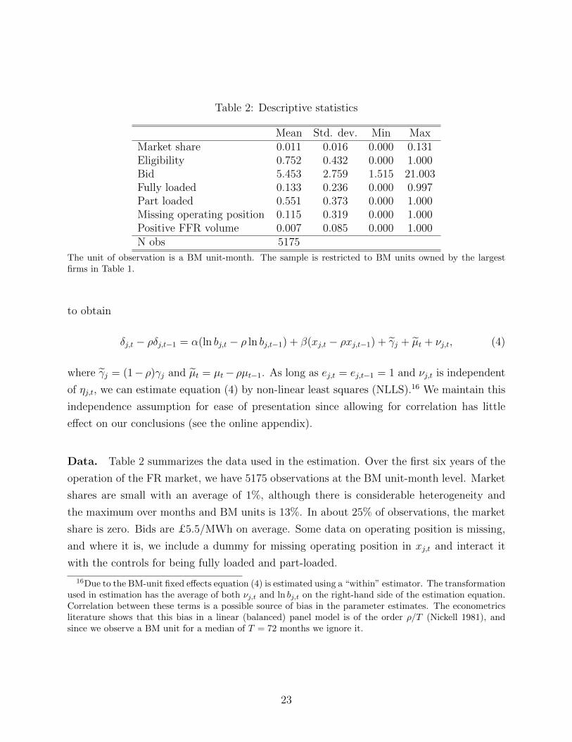
Data. Table 2 summarizes the data used in the estimation. Over the first six years of the
operation of the FR market, we have 5175 observations at the BM unit-month level. Market
shares are small with an average of 1%, although there is considerable heterogeneity and
the maximum over months and BM units is 13%. In about 25% of observations, the market
share is zero. Bids are £5.5/MWh on average. Some data on operating position is missing,
and where it is, we include a dummy for missing operating position in xj,t and interact it
with the controls for being fully loaded and part-loaded.
16Due to the BM-unit fixed effects equation (4) is estimated using a “within” estimator. The transformationused in estimation has the average of both νj,t and ln bj,t on the right-hand side of the estimation equation.Correlation between these terms is a possible source of bias in the parameter estimates. The econometricsliterature shows that this bias in a linear (balanced) panel model is of the order ρ/T (Nickell 1981), andsince we observe a BM unit for a median of T = 72 months we ignore it.
OLS and NLLS estimates of logit model for market share and ML estimates of probit model for eligibility. Allmodels include BM-unit and month fixed effects. NLLS estimates allow the unobservable characteristic ξj,tto follow an AR(1) process with autocorrelation coefficient ρ. The unit of observation is a BM unit-month.Standard errors are clustered by BM unit. R2 is for the fit of predicted versus actual market share, omittingobservations with zero share.
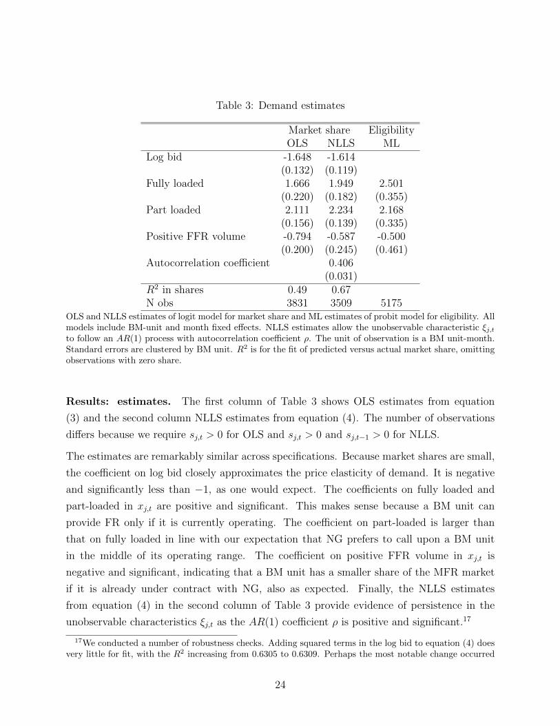
Results: estimates. The first column of Table 3 shows OLS estimates from equation
(3) and the second column NLLS estimates from equation (4). The number of observations
differs because we require sj,t > 0 for OLS and sj,t > 0 and sj,t−1 > 0 for NLLS.
The estimates are remarkably similar across specifications. Because market shares are small,
the coefficient on log bid closely approximates the price elasticity of demand. It is negative
and significantly less than −1, as one would expect. The coefficients on fully loaded and
part-loaded in xj,t are positive and significant. This makes sense because a BM unit can
provide FR only if it is currently operating. The coefficient on part-loaded is larger than
that on fully loaded in line with our expectation that NG prefers to call upon a BM unit
in the middle of its operating range. The coefficient on positive FFR volume in xj,t is
negative and significant, indicating that a BM unit has a smaller share of the MFR market
if it is already under contract with NG, also as expected. Finally, the NLLS estimates
from equation (4) in the second column of Table 3 provide evidence of persistence in the
unobservable characteristics ξj,t as the AR(1) coefficient ρ is positive and significant.17
17We conducted a number of robustness checks. Adding squared terms in the log bid to equation (4) doesvery little for fit, with the R2 increasing from 0.6305 to 0.6309. Perhaps the most notable change occurred
24
The third column of Table 3 shows ML estimates from equation (2). They echo our logit
model for market shares. In particular, the coefficients on fully loaded and part-loaded are
positive and significant, indicating that a BM unit is more likely to be eligible for providing
FR services if it is up and running.
Results: goodness of fit. To assess goodness of fit, we predict the market share of BM
unit j in month t conditional on sj,t > 0. To do so, we sample independently and uniformly
from the empirical distribution of residuals ξj,t for the OLS specification in equation (3) and
from the empirical distribution of residuals νj,t for the NLLS specification in equation (4).18
In both cases we repeatedly sample to integrate out over the empirical distribution of residu-
als. The logit model fits the data reasonably well. Comparing the realized with our predicted
market shares from equation (3) and equation (4), we obtain an R2 of 0.49 and 0.67. This
reinforces the importance of persistence in the unobservable characteristics ξj,t and prompts
us to take the NLLS estimates from equation (4) in the second column of Table 3 as our
leading estimates.19
Figure 12 shows that the fit is good even for the largest power stations, whose market shares
change quite dramatically from one month to the next. The fact that predicted market
shares closely track actual market shares over time makes it clear that the good fit is not
solely a consequence of having BM-unit fixed effects.
when we instrument for ln bj,t with its lag ln bj,t−1. The estimate for α decreases from −1.614 in the middlecolumn of Table 3 to −1.801. While the estimate for α decreases, the estimate for β remains virtuallyunchanged. We find the same when we additionally instrument with the second lag ln bj,t−2. These changesare not large enough to affect our conclusions.
18In the latter case, we proceed as follows: We first obtain the residuals νj,t along with the estimated
parameters α and β from equation (4). We then rewrite equation (3) as δj,t−α ln bj,t−βxj,t = γj +µt+ ξj,t,
substitute in α and β, and estimate by OLS. This yields the residuals ξj,t along with the estimated BM-unit
and month fixed effects γj and µt. We simulate ξj,t by substituting ξj,t−1 and a draw from the empiricaldistribution of residuals νj,t into the law of motion ξj,t = ρξj,t−1 + νj,t. If BM unit j has a zero share inmonth t− 1 so ξj,t−1 is missing, then we go back to the first month τ1 < t− 1 such that sj,τ1 > 0 and we goforward to the first month τ2 > t− 1 such that sj,τ2 > 0. We assume that νj,l = ν for all l = τ1, . . . , τ2 and
solve the equations ξj,t−1 = ρt−1−τ1ξj,τ1 + ν∑t−1−τ1−1l=0 ρl and ξj,τ2 = ρτ2−t+1ξj,t−1 + ν
∑τ2−tl=0 ρl for ν and
ξj,t−1. If missing for a stretch at the beginning so that τ1 is not defined, then we use the second equationalone with ν = 0; if missing for a stretch at the end so that τ2 is not defined, then we use the first equationalone with ν = 0.
19As we pointed out in Section 2, the demand for and supply of FR are relatively stable over most of thesample period. As noted by a referee, this may seem surprising in light of the advent of wind and solarpower. To investigate further, we computed the standard deviation of the residuals νj,t across BM units overtime. There was no discernible increase in volatility over the sample period.
25
.1.2
.3.4
.5S
hare
2005−11 2007−04 2008−10 2010−04 2011−10Date
DRAXX
0.0
5.1
.15
.2.2
5S
hare
2005−11 2007−04 2008−10 2010−04 2011−10Date
EGGPS0
.05
.1.1
5.2
Sha
re
2005−11 2007−04 2008−10 2010−04 2011−10Date
RATS
0.0
5.1
.15
.2S
hare
2005−11 2007−04 2008−10 2010−04 2011−10Date
BARK
Figure 12: Goodness of fit. Realized (blue, solid) and predicted (red, dashed) market shareby month for the four largest power stations Drax (top left panel), Eggborough (top rightpanel), Ratcliffe (bottom left panel), and Barking (bottom right panel).
4.2 Cost
Since the firms we are modeling have been providing FR for a long time, we assume that
they know their own cost (but not necessarily those of their rivals). The cost of providing
FR is not known to us, however, and we have to estimate it as an input to the learning
models in Section 5.
The main source of cost is the additional wear and tear that a BM unit incurs while in FR
mode, which we expect to be relatively stable over time. Let cj denote the constant marginal
cost of BM unit j for providing FR. The realized profit of firm i in month t is
πi,t =∑j∈Ji
(bj,t − cj)Mtsj(bt, xt, ξt, et; θ0), (5)
26
where Mt is market size in month t. The market share of BM unit j in month t depends
on the bids bt, characteristics xt and ξt, and eligibilities et, of all BM units, as well as on
the true parameters θ0 of the demand system. In contrast to market share, market size
Mt is independent of bids bt because the response requirement NG is obligated to satisfy is
exogenously determined by government regulation as a function of the demand for electricity.
We estimate the marginal cost ci = (cj)j∈Ji for the BM units that are owned by firm i from
the bidding behavior of the firm in the late or stable-price phase of the FR market from
June 2009 to October 2011. We maintain that a firm’s bidding behavior stems from the firm
“doing its best” in the sense of choosing its bid to maximize its expected profit conditional
on the information available to it. More formally, the bids bi,t of firm i in month t ≥ 44
maximize the firm’s perception of expected profit conditional on the information it has at
its disposal at the time the bid is submitted:
maxbi,tEb−i,t,ξt,et,θt
[∑j∈Ji
(bj,t − cj)Mtsj(bt, xt, ξt, et; θt)
∣∣∣∣Ωi,t−1
], (6)
where, in a slight abuse of notation, we use Ωi,t−1 to denote both the firm’s perceptions and
the information used to form these perceptions. The notation in equation (6) is designed to
stress the two main sources of uncertainty that a firm faces, namely (i) strategic uncertainty
about its rivals’ bids b−i,t and (ii) demand uncertainty generated by the realizations of ξt
and et and the fact that the parameters θt of the demand model may not be known (so to
the firm the demand parameters are a random variable). Using the information available
to it, the firm forms perceptions about b−i,t, ξt, et, and θt, and these perceptions may
change over time as more information becomes available.20 These perceptions underlie the
expectation operator Eb−i,t,ξt,et,θt [·|Ωi,t−1] in equation (6). How perceptions are formed is the
central question for the learning models that we turn to in Section 5, but for now we remain
agnostic.
Equation (6) implies that the firm believes its current bids do not impact future profit, and
because of this rules out most models of experimentation. It is therefore not an appropriate
characterization of the bidding behavior in the early phase of the FR market. It also rules
out collusive equilibria, since in that case firms act to maximize a different objective function.
20We make the simplifying assumption that the firm has perfect foresight about market size Mt and thecharacteristics xt to avoid modeling their perceptions about these objects. Our estimates do not depend onthis assumption in any way because our approach is robust to Mt and xt being unknown to the firm. Incontrast, our analysis of learning and equilibrium in Section 5 relies on this assumption.
27
We come back to the possibility of collusion below.
Equation (6) implies that the bids bi,t of firm i in month t ≥ 44 solve the first-order conditions
Eb−i,t,ξt,et,θt
[Mtsk(bt, xt, ξt, et; θt) +
∑j∈Ji
(bj,t − cj)Mt∂sj(bt, xt, ξt, et; θt)
∂bk,t
∣∣∣∣Ωi,t−1
]= 0, ∀k ∈ Ji.
(7)
Since we have not specified how the firm forms its perceptions, the system of first-order
conditions in equation (7) cannot be used directly to estimate marginal cost ci. Instead, we
find our estimate of ci by first substituting the realized market size Mt and market shares
si,t = (sj,t)j∈Ji for the BM units that are owned by firm i as well as our estimate α from
Table 3 into equation (7) and then setting the time-average of the first-order conditions for
months t ≥ 44 to zero:
1
29
T=72∑t=44
[Mtsk,t +
∑j∈Ji
(bj,t − cj)Mt (1(k = j)− sk,t)αsj,tbk,t
]= 0, ∀k ∈ Ji, (8)
where we have substituted out for the derivatives in equation (7) using the properties of
the logit and 1(·) is the indicator function.21 We estimate ci by solving this system of |Ji|equations for the |Ji| unknowns. This is straightforward because the equations are linear in
the unknowns.
This estimation approach requires that firms are rational in the following sense: a firm makes
no systematic mistakes in how it perceives its first-order conditions. This implies that the
time-average of the firm’s perceptions of its first-order conditions is zero, and this in turn
implies that equation (8) holds asymptotically as the time horizon T → ∞. We view this
weak rationality assumption — due to Pakes (2010) and also used in Fershtman and Pakes
(2012) — as appropriate for the late phase of the FR market, since by the time the FR
market enters the late phase, firms have had ample opportunity to observe how their rivals
bid as well as the resulting allocation of market shares. Changes in cost or cyclicality in
demand do not invalidate the estimation approach, as long as they do not cause firms to
start making systematic mistakes i.e. as long as firms adjust to changes in the environment.
21If a firm does not have perfect foresight about market size, Mt cannot generally be canceled out ofequations (7) and (8) as market size and market share may be correlated. At the suggestion of a referee, weprovide a robustness check in the online appendix where we cancel Mt out, and show that the cost estimateswe obtain are uniformly close to those in the main text.
28
The weak rationality assumption is less demanding than assuming (as the industrial orga-
nization literature often does) that firms are playing a Nash or Bayes-Nash equilibrium.
Any “rational expectations” equilibrium requires that firms’ perceptions about the payoffs
to different actions are correct along the path of equilibrium play. By contrast, this esti-
mation approach does not require assuming that the market is in equilibrium or that the
environment necessarily reaches some sort of rest point, it may be useful for empirical work
in other contexts. In the appendix, we provide sufficient conditions for obtaining consistent
cost estimates.
Results: estimates. The average of the marginal cost cj that we estimate for the J = 72
BM units owned by the ten largest firms is £1.40/MWh, with a standard deviation of
£0.66/MWh across BM units.22 The estimates are reasonably precise, with an average
standard error of £0.04/MWh. By comparison, pre CAP047 the “cost reflective” adminis-
tered price was around £1.7/MWh.23 Since we expect some markup to be built into the
administered price, the marginal costs we recover are in the right ballpark.
Table 4 shows the average marginal cost for the BM units belonging to the eight largest
power stations. It is quite reasonable and varies between £1.04/MWh and £1.59/MWh
across stations. The standard deviation of marginal cost within a station is very small, on
the same order as the standard error of the estimates. Most of the variation in marginal cost
is therefore across stations. This is in line with the fact that the BM units belonging to the
same station tend to be identical.
Table 5 shows the result of regressing marginal cost on the characteristics of the BM units.
As expected, a (typically smaller) BM unit using dual fuel or oil has lower cost than a BM
unit using other fuel types. Moreover, although not statistically significant, the estimates
suggest that a BM unit of later vintage has lower cost.
Results: residuals. Using our estimates, we evaluate realized values of the profit deriva-
tive Mtsk,t +∑
j∈Ji (bj,t − cj)Mt (1(k = j)− sk,t) αsj,tbk,t
in equation (8) for each BM unit and
22Because one BM unit has zero share during the late phase, we impute its marginal cost with that of theother BM unit in the same power station.
23We have two sources: Figure 2 and a document prepared just prior to CAP047 by NG for Ofgem, thegovernment regulator. (www.ofgem.gov.uk/ofgem-publications/62273/8407-21104ngc.pdf). It statesin paragraph 5.3 that the holding payment is “of the order of £5/MWh” for the bundle of primary, secondary,and high response, implying an average of £1.67/MWh per type of FR.
29
Table 4: Marginal cost estimates for the largest power stations
Characteristics of power station and average and standard deviation of marginal cost estimate cj across BMunits within station. Stations ranked by revenue in the FR market during early and middle phases.
month. For simplicity, we call this value a “residual.” The average of this residual over the
late phase of the FR market is zero for all BM units by construction. Figure 13 shows the
time series of the average residual across BM units. It contrasts the early and middle phases
in the left panel with the late phase of the FR market in the right panel (for visual clarity,
we scale the vertical axis differently in the two panels).
The average residual starts well above zero in the early phase before falling below zero in the
middle phase. The standard deviation falls throughout, consistent with our earlier discussion
of convergence. In the late phase, the average residual is above zero in some months and
below zero in others and the standard deviation does not exhibit a trend. Interestingly, even
after the substantial increase in FFR volume that occurs in July 2010 (see Figure 4; July
2010 is marked with a dotted line in the right panel of Figure 13) and changes in participation
during this phase (see Figure 5), the standard deviations of the residual are still an order of
magnitude smaller than in the earlier phases of the FR market.
We also examined whether the residuals are autocorrelated. The first three columns of
Table 6 display the coefficients from separate regressions of the residual on its lagged value for
each of the three phases of the FR market, including BM-unit fixed effects in all regressions.
In the last three columns we further restrict attention to observations in which the BM unit’s
bid changed between months.
We find significant autocorrelation in all regressions but the last. Assuming our specification
and cost estimates are correct, this indicates that some firms are making mistakes that are
not corrected in the subsequent month. This may reflect persistent differences between a
30
Table 5: Marginal cost estimates and BM-unit characteristics
CoefficientUnit vintage -0.015
(0.017)Dual fuel -0.819
(0.466)Large coal -0.463
(0.429)Medium coal -0.683
(0.544)Oil -0.967
(0.397)R2 0.13N obs 71
Regression of marginal cost estimate cj on characteristics of BM unit. The omitted fuel type is combinedcycle gas turbines (CCGT). The unit of observation is a BM unit. One observation is dropped because ofmissing vintage.
firm’s perceptions of its expected profits and reality, an interpretation that makes particular
sense in the early and middle phases of the FR market where firms had little experience and
behaved quite differently. Relatedly it is striking how the R2 falls over the three phases of
the FR market, indicating that the lagged value explains progressively less of the variation in
the residual. In the third phase, we still find significant autocorrelation using all observations
(third column), but that autocorrelation essentially disappears when we restrict attention
to observations in which the BM unit’s bid changed between months (last column). Our
interpretation of this is that by the third phase firms have reasonably accurate perceptions,
but do not always update their bid. When they do choose to update their bid, they do so
in a way that accounts for the information contained in the lagged residual.
Robustness check: fuel price. As noted in Section 2, there is an upward trend in oil and
— to a lesser extent — gas prices towards the end of the sample period. While the major cost
of providing FR is additional wear and tear, a BM unit in FR mode may run with a degraded
heat rate. Hence, the cost of providing FR may be tied to the fuel price. As a robustness
check, we model the marginal cost of BM unit j in month t as cj,t = cj + µfj,t, where cj is a
BM-unit fixed effect, fj,t is the fuel price that the BM unit faces, and µ is a parameter to be
estimated. In the online appendix we provide details on how we accommodate the additional
31
050
0010
000
2005−07 2006−07 2007−07 2008−07 2009−07Date
Average residual Standard deviation of residuals
−10
000
1000
2000
3000
2009−07 2010−01 2010−07 2011−01 2011−07Date
Average residual Standard deviation of residuals
Figure 13: Average and standard deviation of residuals during the early and middle phases(left panel) and late phase (right panel). In the right panel, the dotted line indicates July2010, when FFR volume nearly doubles.
Table 6: Autocorrelation in residuals
All Only bid changesEarly Middle Late Early Middle Late
Separate regressions of residual on lagged residual for the three phases of the FR market. All regressionsinclude BM-unit fixed effects. The unit of observation is a BM unit-month. The first three regressions useall observations. The last three regressions are restricted to observations in which a BM unit’s bid changedbetween months. Standard errors are clustered by BM unit.
parameter in the estimation. We find that µ is negative and significant but economically
small. The negative sign appears inconsistent with the intuition that a BM unit in FR mode
consumes more fuel. We therefore re-estimated cost allowing for a time trend (with and
without the fuel price) and found that the impact of the fuel price is indistinguishable from
a downward time trend. So there may be something changing cost over time in our data,
but it is not necessarily related to the fuel price. To ensure that the downward time trend
does not affect our results, we re-ran the analysis of the learning models in Section 5 with
the alternative specification of cost. As documented in the online appendix, our conclusions
remain unchanged.
32
Robustness check: repositioning in the BM. One might worry that equation (5)
does not reflect the full set of incentives a firm faces, as it does not account for the profit
that accrues to a BM unit as it is repositioned in the BM in preparation for providing
FR. In the online appendix, we incorporate these incentives. Using additional data on the
BM, we first model and estimate demand for repositioning. Extending equation (8), we then
simultaneously estimate the marginal cost of providing FR and the markup on repositioning.
The estimated markup is very small and not statistically different from zero, and the marginal
cost of providing FR does not change materially from that reported earlier in this section.
The markup partly reflects the amount of attention paid to the profit from repositioning
when deciding on the FR bid. Our estimate may thus be explained by the fact that FR bids
and bids in the BM are made by different people within the firm, and those deciding on FR
bids may not pay attention to the BM. This is consistent with our conversations with Ian
Foy, who told us that people in the industry do not think of repositioning incentives when
deciding on FR bids.24
Robustness check: collusion. We finally turn to the possibility that firms collude and
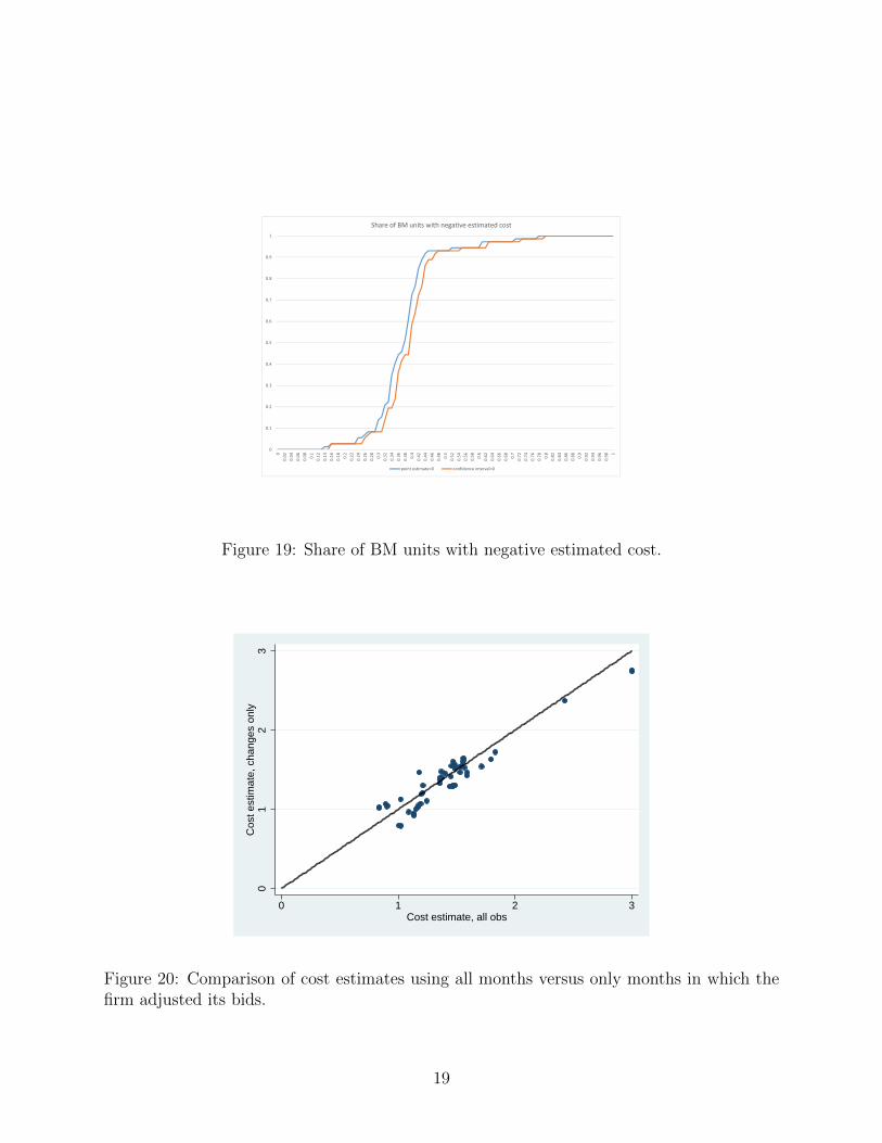
that equation (5) is therefore misspecified. In the online appendix, we try three different
ways of examining the data for evidence of collusion. The first is to examine whether bid
changes across BM units owned by different firms are correlated in either timing or direction.
The pairwise correlations are symmetrically distributed around zero (whereas the within-firm
correlations are virtually all positive). This is incompatible with most models of coordinated
pricing, though it is possible that an unknown subset of firms collude and that there is
correlation within that subset. Our second approach is more direct. We assume particular
collusive arrangements and infer cost given the assumed conduct. Our estimate of marginal
cost becomes negative, which we take as evidence against these arrangements. Finally, at
the suggestion of a referee, we ask how much weight the firms can put on their rivals’ profits
when optimizing their bids while ensuring that the observed bids are consistent with non-
negative cost. We find that the maximum weight is relatively small. Thus in all three
approaches, we find little evidence of collusion, which is perhaps not surprising in view of
the mild concentration of the FR market.
24A possible explanation may be that the compensation of different employees is tied to different markets.We thank an anonymous referee for pointing this out.
33
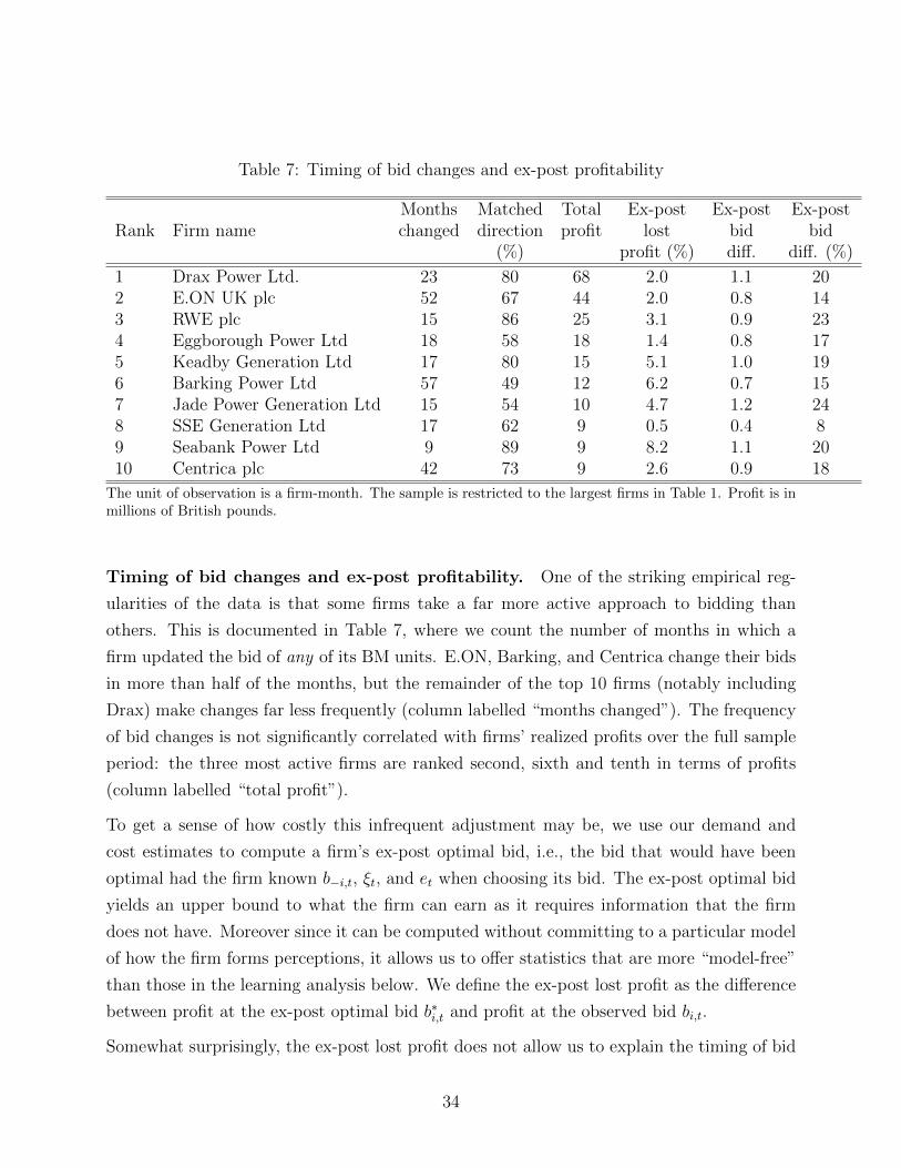
Table 7: Timing of bid changes and ex-post profitability
Months Matched Total Ex-post Ex-post Ex-postRank Firm name changed direction profit lost bid bid
The unit of observation is a firm-month. The sample is restricted to the largest firms in Table 1. Profit is inmillions of British pounds.
Timing of bid changes and ex-post profitability. One of the striking empirical reg-
ularities of the data is that some firms take a far more active approach to bidding than
others. This is documented in Table 7, where we count the number of months in which a
firm updated the bid of any of its BM units. E.ON, Barking, and Centrica change their bids
in more than half of the months, but the remainder of the top 10 firms (notably including
Drax) make changes far less frequently (column labelled “months changed”). The frequency
of bid changes is not significantly correlated with firms’ realized profits over the full sample
period: the three most active firms are ranked second, sixth and tenth in terms of profits
(column labelled “total profit”).
To get a sense of how costly this infrequent adjustment may be, we use our demand and
cost estimates to compute a firm’s ex-post optimal bid, i.e., the bid that would have been
optimal had the firm known b−i,t, ξt, and et when choosing its bid. The ex-post optimal bid
yields an upper bound to what the firm can earn as it requires information that the firm
does not have. Moreover since it can be computed without committing to a particular model
of how the firm forms perceptions, it allows us to offer statistics that are more “model-free”
than those in the learning analysis below. We define the ex-post lost profit as the difference
between profit at the ex-post optimal bid b∗i,t and profit at the observed bid bi,t.
Somewhat surprisingly, the ex-post lost profit does not allow us to explain the timing of bid
34
changes. While we expect firms to be more likely to adjust their bids in months where the
ex-post lost profit is large, we find no statistically significant support for this in any of a
number of probit regressions that explore different plausible specifications.25
The ex-post optimal bid helps to explain the direction in which firms adjust their bids,
conditional on adjusting. The column labelled “matched direction” in Table 7 indicates the
percentage of times that such adjustments are in the direction of the ex-post optimal bid
(share-weighted across the BM units within a firm). It is well above 50% for many firms.
For the most active firms we match the direction less often, consistent with our account of
firms “exploring” during the early phase of the FR market. The percentage of matches is at
most weakly correlated with firm size as measured by realized profit over the sample period:
the four highest percentages are ranked ninth, third, first, and fifth in terms of firm size.
This seems different than Hortacsu and Puller’s (2008) finding that firms with large stakes
made bids that were closer to optimal in the electricity spot market in Texas.
To measure how much money the firms have “left on the table” we look at the ex-post lost
profit over the full sample period as a percentage of realized profit in the column labelled
“ex-post lost profit (%)” of Table 7. The magnitudes are generally small. For example, RWE
plc rarely updated its bids and slowly tracked the market upwards. As a result, we estimate
that they lost £768,000 or 3.06% over six years. While this is enough money that we may
expect RWE plc to pay more attention and update its bids more frequently, it is perhaps not
enough to justify hiring a full-time employee to study the FR market and optimize bidding.
Contrast these small ex-post profit differences with the average absolute difference between
a firm’s (share-weighted) average bid and the ex-post optimal bid, shown in the last two
columns labelled “ex-post bid difference” and “ex-post bid difference (%)” in absolute and
relative terms. These magnitudes are much larger, with most firms placing bids that are
around 15% to 20% away from their ex-post optimal bids.
This suggests a possible reason why we have been unable to explain the timing of bid changes:
once one allows for the uncertainty which the ex-post optimal bid abstracts from, it may
not be obvious to a firm that adjusting its bid increases its profit in any substantial way.26
25We note that this makes it unlikely that switching costs are the root cause for the infrequent adjustmentsto bids, as most models with switching costs predict bid changes exactly at times when the perceived gainsto adjustment are largest. Despite our skepticism of these models, we provide alternative cost estimates inthe online appendix that are consistent with a very simple model of switching costs or inattention; these lineup closely with our leading estimates.
26The fact that profit is not overly sensitive to a deviation from the ex-post optimal bid may have length-ened the time it took the FR market to reach a rest point. The lack of sensitivity may have implied a
35
Yet, as Akerlof and Yellen (1985) have noted — and as our study seems to illustrate — even
small departures from perfectly rational behavior may lead to aggregate behavior that is
quite different from equilibrium. To further investigate this disequilibrium bidding behavior,
we use learning models.
5 Learning and equilibrium
In this section we consider how well different learning models fit the data. We noted in
Section 3 that realistically accounting for the bidding behavior in the early phase of the FR
market requires an explanation for the heterogeneity in the way firms learn and a model that
allows for experimentation. These are topics we do not tackle here. Instead, we consider
models of the bidding behavior in the middle and late phase of the FR market. The middle
phase is characterized by a convergence of bids in a relatively stable environment whereas
there are several environmental changes in the late phase.
Our learning models capture the two main sources of uncertainty that a firm faces, namely
(1) strategic uncertainty about its rivals’ bids b−i,t, and (2) demand uncertainty generated
both by the realizations of ξt and et and by the fact that the parameters θ of the logit model
may not be known. As noted in Section 1, the literature traditionally uses different types
of models for how a firm forms perceptions about rivals’ bids and for how the firm forms
perceptions about demand, and so do we. Our learning models combine fictitious play as a
model for learning about rival’s bids with adaptive learning about demand.
Recall that prior to CAP047 providing FR was mandatory, so at the start of our study firms
already had quite a bit of experience with demand and cost. We therefore assume throughout
that firms know the marginal cost c of all BM units, the AR(1) process generating ξt, the
objective probability distribution of et, and the BM-unit fixed effects γ = (γj)j=1,...,J . The
latter capture the time-invariant preferences of NG for the different BM units. However, there
is reason to think firms had to learn about other aspects of demand. In particular, since
prior to CAP047 the holding payment was at an administered price which had been fairly
constant over time, firms may not have been able to assess the sensitivity of NG to the bids
they submit, a sensitivity captured by the parameter α in our model. They may also have
been uncertain about the parameter β to the extent that the time-varying characteristics
combination of rational inattention (Sims 2003) and satisficing behavior (Simon 1955) that may have beenoptimal along the observed path of play given firms’ various human resource and institutional constraints.
36
xj,t mattered differently for NG post CAP047. Finally, firms may have been uncertain about
the month fixed effects µ = (µt)t=1,...,72 that subsume any time-varying characteristics of the
outside good.
As a baseline we also compute a complete information Nash equilibrium. This is the leading
model in the empirical industrial organization literature, so how it compares to our learning
models is of some interest.
5.1 Complete information Nash equilibrium
The assumptions underlying a complete information Nash equilibrium are more restrictive
than those we needed to estimate cost. Formally, the bids b∗t of all BM units satisfy the
system of J equations
Eξt,et
[Mtsk(b
∗t , xt, ξt, et; θ0)
+∑j∈Ji
(b∗j,t − cj
)Mt
∂sj(b∗t , xt, ξt, et; θ0)
∂bk,t
∣∣∣∣Mt, xt, ξt−1, θ0, c
]= 0, ∀k = 1, . . . , J. (9)
The notation Eξt,et [·|·] in equation (9), in contrast to Eb−i,t,ξt,et,θt [·|·] in equation (6), is
meant to indicate that the expectation is computed with respect to the objective probability
distribution of ξt and et conditional on the information available to firm i in month t − 1
when it submits its bids bi,t for month t. We assume that the firm has perfect foresight
about market size Mt and the observable characteristics xt. In addition, we condition the
expectation operator on the unobservable characteristics ξt−1 with the implicit understanding
that ξj,t follows the AR(1) process ξj,t = ρξj,t−1 + νj,t with ρ known. Finally, we abstract
from uncertainty about the parameters of the demand system for now and condition the
expectation operator on θ0. Later on we extend the complete information Nash equilibrium
to accommodate adaptive learning about demand.
Note that the expectation operator in equation (9) does not condition on b−i,t. While the
best response of firm i depends on its perceptions of its rivals’ bids, in a complete information
Nash equilibrium these perceptions are consistent with actual play. A complete information
Nash equilibrium is thus obtained by solving the above J equations in the J unknowns b∗t .
We are not aware of a result in the extant literature that shows that there is a unique
37
complete information Nash equilibrium in our setting. However, we have checked extensively
for multiplicity by trying different starting points for the equation solver and never found
more than one complete information Nash equilibrium.
To make equation (9) practical we replace ξt−1, θ0, and c by our estimates of those objects and
evaluate the expectation operator using Monte Carlo integration. To this end we generate a
random sample(ξ
(s)t , e
(s)t
)s=1,...,S
with S = 50, 000 and replace the expectation operator by
the corresponding sample average. To obtain ξ(s)j,t , we sample independently and uniformly
from the empirical distribution of residuals νj,t from the NLLS specification in equation (4)
(for further details see footnote 18). To obtain e(s)j,t , we sample independently from a Bernoulli
distribution with success probability Pr(ej,t = 1|xj,t) as specified in equation (2).
5.2 Learning models
We now turn to the learning models we use for firms’ perceptions about rivals’ bids and
demand.
Perceptions about rivals’ bids: fictitious play. Belief-based learning starts with the
premise that players keep track of the history of play and form beliefs about what their
rivals will do in the future based on their past play. We consider fictitious play as a leading
example of belief-based learning.27 In particular, we assume that in month t− 1 when firm
i chooses its bids bi,t it believes that its rivals’ bids b−i,t are sampled from the empirical
distribution of their past play. To account for correlation in the bids of firm i’s rivals, we
sample an entire vector of rivals’ bids. Since firm i may believe that its rivals’ bids b−i,t are
likely to be more similar to more recent observations, we allow for geometrically declining
sampling weights. In particular, we assign sampling weight δt−τ−1 to rivals’ bids b−i,τ in
month τ ≤ t− 1, where δ ∈ [0, 1] is a decay parameter, and then normalize so the sampling
weights sum to one. For month τ = t − 1, t − 2, t − 3, . . . the sampling weight is therefore
proportional to 1, δ, δ2, . . ..28
We let F (δ) denote our model of fictitious play with decay parameter δ. Note that δ = 1
indicates no decay and δ = 0 full decay. Under F (0) firm i believes that its rivals’ bids b−i,t
27For a discussion of fictitious play and its variants see Fudenberg and Levine (1998).28In nine instances the bid bj,t of BM unit j in month t is missing. To facilitate sampling, we impute it
by going back in time to the first month τ < t such that bj,τ is not missing.
38
in month t are equal to its rivals’ bids b−i,t−1 in month t − 1 with certainty. Adaptive best
response thus arises as a special case of fictitious play with δ = 0. In the other extreme,
under F (1) all past observations are weighted equally.29
Perceptions about demand: adaptive learning. To account for uncertainty about de-
mand in addition to uncertainty about rivals’ bids, we allow a firm to adaptively learn about
the parameters θ of the logit model. Developed in the macroeconomics literature, adaptive
learning stipulates that agents learn about parameters in the same way as econometricians
do, by using the available data to estimate them. As more data becomes available over time,
agents update their estimates.30
We focus on a simple form of adaptive learning that assumes that firms use the regression
procedure described in Section 4.1 and the data available to them to estimate the parameters
they are uncertain about. In month t−1, when firms prepare their bids for month t, firms only
have data for month τ ≤ t− 2 at their disposal (NG does not publish quantities for a month
until the very end of the month). We refer to the estimates obtained in this manner as the
“sequential” estimates for month t and distinguish them from the “full-sample” estimates
obtained in Section 4.1. We assume throughout that firms ignore any uncertainty in the
sequential estimates so that their perceptions put point mass on those estimates.
We noted above that there is reason to think that firms may have been uncertain about the
price sensitivity parameter α, the coefficient β on the time-varying characteristics xj,t, and
about the month fixed effects µ. Accordingly, we distinguish four combinations of parameters
that firms may have been uncertain about, namely: α, α and β, α and µ, and α, β, and
µ. Our notation for and implementation of adaptive learning for these four cases plus the
baseline case that abstracts from demand uncertainty follows:
1. A(α): Using data for month τ ≤ t − 2 and fixing β, ρ, γ, and (µτ )τ≤t−2 at the full-
sample estimates in Table 3, estimate equation (4) by OLS to obtain the sequential
estimate α(t) for month t.
29The decay parameter δ implicitly also determines the variance of a firm’s beliefs about its rivals’ bids.In particular, the variance vanishes as δ approaches zero. While this is a feature of the fictitious play modelsused in the theory and experimental literatures, a fruitful avenue for future research may be to considerother learning models that disentangle the variance of a firm’s beliefs from the weight the firm assigns tothe more distant past.
30For a detailed treatment of adaptive learning see Evans and Honkapohja (2001).
39
2. A(α, β): Using data for month τ ≤ t − 2 and fixing ρ, γ, and (µτ )τ≤t−2 at the full-
sample estimates, estimate equation (4) by OLS to get the sequential estimates α(t)
and β(t) for month t.
3. A(α, µ): Using data for month τ ≤ t − 2 and fixing β, ρ, and γ at the full-sample
estimates, estimate equation (4) by OLS to obtain the sequential estimates α(t) and(µ(t)
τ
)τ≤t−2
for month t. Using data for month τ ≤ t − 2 and fixing β and γ at the
full-sample estimates and α at the sequential estimate for month t, estimate equation
(3) by OLS to obtain the sequential estimates(µ
(t)τ
)τ≤t−2
(for more details see footnote
18). Extrapolate µ(t)t = µ
(t)t−2 to obtain the sequential estimate µ
(t)t for month t.
4. A(α, β, µ): Using data for month τ ≤ t − 2 and fixing ρ and γ at the full-sample
estimates, estimate equation (4) by OLS to obtain the sequential estimates α(t), β(t),
and
(µ(t)
τ
)τ≤t−2
for month t. Using data for month τ ≤ t− 2 and fixing γ at the full-
sample estimate and α and β at the sequential estimates for month t, estimate equation
(3) by OLS to obtain the sequential estimates(µ
(t)τ
)τ≤t−2
. Extrapolate µ(t)t = µ
(t)t−2 to
obtain the sequential estimate µ(t)t for month t.
5. A(∅): Fix all parameters θ at the full-sample estimates in Table 3 to abstract from
demand uncertainty.
Figure 14 illustrates the sequential estimates. The left panel shows α(t) obtained alternatively
under A(α) and A(α, β) and the right panel shows β(t) obtained under A(α, β). Over time the
sequential estimates by construction approach the full-sample estimates obtained in Section
4.1. The sequential estimates for the price sensitivity parameter α start out small in absolute
value and gradually decrease. Until the late phase of the FR market, α(t) is considerably
smaller under A(α) than under A(α, β). The sequential estimate produced by A(α) is within
2% of the full sample estimate by the start of the middle phase; apparently the variance in
prices in the initial phase enabled reasonably accurate estimates of the price coefficient by
the beginning of the middle phase. The sequential estimate β(t) on positive FFR volume
is far from its full-sample estimate until month 25 (because there is little FFR volume in
the early part of the data), but stabilizes thereafter. The sequential estimates β(t) on part-
loaded and fully loaded are much less volatile and gradually trend towards their full-sample
estimates.
40
-1.6
-1.5
-1.4
-1.3
-1.2
-1.1
Estim
ated
Pric
e C
oeffi
cien
t (Al
pha)
2005-11 2007-04 2008-10 2010-04 2011-10Date
Alpha estimates, only alpha unknownAlpha estimates, alpha and beta unknown
-3-2
-10
12
Est
imat
ed C
oeffi
cien
t
2005-11 2007-04 2008-10 2010-04 2011-10Date
Coefficient on Fully LoadedCoefficient on Part LoadedCoefficient on FFR Contract
Figure 14: Sequential estimates α(t) under A(α) and A(α, β) (left panel) and β(t) underA(α, β) (right panel) by month.
Predictions. We combine fictitious play with adaptive learning to make predictions. We
measure fit by comparing our predictions to the observed bids. We make two kinds of
predictions. The first is one-period predictions: for month t during the middle and late
phases of the FR market, we take the data available to the firms at the time they bid (which
includes bids (br)r≤t−1 and market shares (sr)r≤t−2) and predict their bids. This corresponds
to the thought experiment of predicting the next move of a player in a game and is analogous
to the one-step-ahead predictions used to assess predictive accuracy in the experimental and
computational literatures (Erev and Roth 1998, Fershtman and Pakes 2012).
However, industrial organization analysts are often asked to predict how prices evolve for
many periods following a policy change or a change in market institutions. We therefore also
consider multi-period predictions in which we sequentially predict bids and market shares
and then overwrite the observed data with our predictions as we go. To see how these differ,
consider the following example: if the strategic model specifies that firms best respond to last
period’s bids, and we predict in period t that BM unit 1 bids 7 but it actually bids 11, then in
the one-period prediction exercise we predict that in period t+1 the other firms best respond
to the actual bid of 11, but in the multi-period prediction exercise they best respond to the
predicted bid of 7. This allows the possibility that our multi-period predictions increasingly
diverge from the observed data. Indeed, if the model is correct, then the variance of the
prediction error should grow with the distance between the base period and the period for
which we are predicting.
41
A fictitious play model F (δ) with δ ∈ [0, 1] and an adaptive learning model A(y) with
y ∈ α, (α, β), (α, β, µ), ∅ together with available data Dt determine a predicted bid b(δ,y)i,t
for firm i in month t. That bid b(δ,y)i,t solves the system of Ji equations
Eb−i,t,ξt,et,θt
[Mtsk(b
(δ,y)i,t , b−i,t, xt, ξt, et, θt)
+∑j∈Ji
(b
(δ,y)j,t − cj
)Mt
∂sj(b(δ,y)i,t , b−i,t, xt, ξt, et, θt)
∂bk,t
∣∣∣∣F (δ), A(y), Dt
]= 0, ∀k ∈ Ji. (10)
The notation Eb−i,t,ξt,et,θt [·|·] indicates that the expectation operator is with respect to the
subjective probability distributions of b−i,t and θt induced by F (δ) and A(y). To make
equation (10) practical we replace ξt−1 and c in Dt by our estimates. In the single-period
prediction exercises, we estimate θt for the adaptive learning model A(y) as detailed above
using the observed data for month τ ≤ t − 2. We evaluate the remaining random variables
in the expectation operator by drawing samples(b
(s)−i,t, ξ
(s)t , e
(s)t
)s=1,...,S
with S = 50, 000,
proceeding as in Section 5.1 for sampling ξ(s)j,t and e
(s)j,t . We sample b−i,t from the data
(b−i,τ )τ≤t−1 according to F (δ).
The multi-period prediction exercises are identical except for the data Dt: for any model
(F (δ), A(y)) we replace the observed bids and market shares during the middle and late
phases with our predictions b(δ,y)t , thus changing what firms observe.31 This has two effects.
First, when sampling b−i,t according to F (δ), we now sometimes sample our predicted bids.
Second, when estimating θt, the dataset used for estimation now contains our predicted
bids and market shares. These effects generate differences between the single- and multi-
period predictions. For reasons that will become clear below, for the multi-period prediction
exercises we only consider the adaptive learning models A(∅) and A(α).
5.3 Measures of fit
We consider two different measures of fit. First, we ask how well alternative learning models
and the complete information Nash equilibrium predict the overall cost of the FR market
to NG. Second, we compare the models to each other using the traditional measure of
31To predict market shares we use the estimated parameter vector θ regardless of the adaptive learningmodel A(y), as it is our best guess for that parameter.
42
model performance, namely the mean square prediction error. In this section, we define
our measures of fit and in Section 5.4 we describe how we conduct formal statistical tests.
Throughout we focus on the J = 72 BM units owned by the ten largest firms.
NG’s costs. We measure how well the model (F (δ), A(y)) predicts NG’s costs as
CE(δ,y) =1
T
∑t
CE(δ,y)t =
1
T
∑t
∣∣∣∣∣∑j
(b
(δ,y)j,t − bj,t
) sj,t∑j sj,t
∣∣∣∣∣ .CE(δ,y) is the average across months of the absolute value of the prediction error CE
(δ,y)t .
The actual price of FR paid by NG in month t is∑
j bj,tsj,t∑j sj,t
, while the price predicted
by the model is∑
j b(δ,y)j,t
sj,t∑j sj,t
. Replacing b(δ,y)j,t by b∗j,t, we use CE∗ and CE∗t to denote the
analogous measures for the complete information Nash equilibrium in Section 5.1.
Model performance. We measure the performance of model (F (δ), A(y)) as
MSE(δ,y) =
∑t
∑j
(b
(δ,y)j,t − bj,t
)2
sj,t∑t
∑j sj,t
,
or the weighted average of the square prediction error(b
(δ,y)j,t − bj,t
)2
, where the weightsj,t∑
t
∑j sj,t
is the share of BM unit j in month t in the total share of the inside goods across
months. We again use MSE∗ to denote the corresponding measure for the complete infor-
mation Nash equilibrium.
5.4 Results
We begin with discussing how well different learning models fit the data from the middle
phase of the FR market and then move on to the late phase.
Middle or falling-price phase. Table 8 provides the average absolute prediction error
CE(δ,y) and CE∗ for the middle phase and Table 9 provides the mean square prediction
error MSE(δ,y) and MSE∗. The entries in the table are arranged to reflect our two-way
classification of learning models: the first three rows specify the fictitious play model used to
43
Table 8: Middle phase: Average absolute prediction error CE(δ,y)
Computed from bids predicted by fictitious play model F (δ) or complete information Nash equilibrium (rows)in combination with adaptive learning model A(y) (columns).
Table 9: Middle phase: Mean square prediction error MSE(δ,y)
Computed from bids predicted by fictitious play model F (δ) or complete information Nash equilibrium (rows)in combination with adaptive learning model A(y) (columns).
form perceptions of rivals’ bids, followed by the complete information Nash equilibrium, and
the columns specify the adaptive learning model used to form perceptions of the demand
parameters. The five columns on the left pertain to single-period predictions and the two
columns on the right to multi-period predictions.
Starting with the single-period predictions, the 2 × 2 sub-matrix in the top left corner of
Tables 8 and 9 have the smallest values. Regardless of whether we are concerned with CE(δ,y)
or MSE(δ,y), the preferred model for perceptions about rivals’ bids is either F (0) (full decay
beyond the immediate past, or adaptive best response) or F (0.5) (intermediate decay). The
preferred model for perceptions about demand is either A(∅) (no demand uncertainty) or
A(α) (uncertainty about the price sensitivity parameter α). Both measures of fit noticeably
deteriorate under the adaptive learning models A(α, β), A(α, µ) and A(α, β, µ) that presume
that firms are uncertain about additional demand parameters.32
32One should be careful not to overinterpret the deterioration in fit when we assume that firms must learnabout the month fixed effects µ = (µt)t=1,...,72. As noted in Section 5.2, in month t the firm only has the
data available to estimate µτ for τ ≤ t − 2. We assume that the firm extrapolates by equating µ(t)t with
µ(t)t−2, but there are many alternatives that may well produce some increase in fit.
44
When we searched for a point estimate of the decay parameter δ in the fictitious play model,
we obtained the smallest mean square prediction error at δ = 0.3. However, there was very
little difference in the mean square prediction error when δ took on values between 0 and 0.6.
So we conclude only that the data from the middle phase of the FR market appears to favor
a fictitious play model in which firms rely disproportionately on more recent observations to
form beliefs about rivals’ bids.
The single-period predictions in the five columns on the left of Tables 8 and 9 seem to give
only a slight edge to A(α) over A(∅) (as is suggested by Figure 14). This edge, however,
is accentuated in the multi-period predictions in the two columns on the right. The multi-
period predictions compound differences between the sequential estimates α(t) of the price
sensitivity parameter α that underlie A(α) and the full-sample estimate that underlies A(∅) .
More surprising is how well the multi-period predictions using A(α) do. They have essentially
the same mean square prediction error as the single-period predictions using A(α) and do
just up to 10% worse in terms of the average absolute prediction error. In contrast, the
multi-period predictions using A(∅) do 5% to 10% worse than the single-period predictions
using A(∅) in terms of the mean square prediction error and 50% worse in terms of the
average absolute prediction error.
Perhaps the most striking feature of Tables 8 and 9 is that the fictitious play models F (0) and
F (0.5) outperform the complete information Nash equilibrium. This is more pronounced for
the average absolute prediction error, but clearly noticeable for both measures of fit. Table
10 further illustrates just how different the predictions from the learning and equilibrium
models are. In this table, we specifically compare F (0) and A(∅), i.e. adaptive best response
with the full sample estimate, with the complete information Nash equilibrium. To do this,
we regress of CE(0,∅)t − CE∗t first on a constant (column 1) and then a constant and time
trend (column 2). Columns 3 and 4 show the corresponding regressions when the dependent
variable is instead(b
(0,∅)j,t − bj,t
)2
−(b∗j,t − bj,t
)2, the difference in squared prediction error.
In these regressions, we weigh observations bysj,t∑
t
∑j sj,t
to give greater importance to precise
predictions for BM units with larger market shares.
We find statistically and economically significant differences between the learning model and
equilibrium predictions, both with and without a time trend. Moreover, the regressions that
include a time trend indicate that the difference starts out large and declines over the mid-
dle phase of the FR market, with both the initial difference and the subsequent decrease
clearly significant. We find similar statistically and economically significant differences be-
45
Table 10: Middle phase: Comparison of learning model (F (0),A(∅)) and complete informa-tion Nash equilibrium
CE(0,∅)t − CE∗t
(b
(0,∅)j,t − bj,t
)2
−(b∗j,t − bj,t
)2
Constant -0.194 -0.368 -0.192 -0.631
(0.032) (0.055) (0.088) (0.225)
Time trend 0.013 0.031
(0.003) (0.012)
N obs 27 27 1470 1470
In the first two regressions with CE(0,∅)t − CE∗t as the dependent variable, the unit of observation is a
month. In the last two regressions with(b(0,∅)j,t − bj,t
)2−(b∗j,t − bj,t
)2as the dependent variable, the unit
of observation is a BM unit-month. In the latter, observations are weighted bysj,t∑
t
∑j sj,t
as described in
Section 5.3 and standard errors are clustered by month.
tween the predictions of the other leading learning models (F (0.5), A(∅)), (F (0), A(α)), and
(F (0.5), A(α)) and the complete information Nash equilibrium.
Figure 15 shows the time path of the price of FR paid by NG as predicted by alternative
learning models and the complete information Nash equilibrium as well as the time path of
the actual price of FR (black line). Modulus multiplicity issues, only changes in the demand
and cost primitives can cause changes in the complete information Nash equilibrium. As the
turquoise line in Figure 15 shows, these changes alone do not allow the complete information
Nash equilibrium to vary sufficiently to track the actual price of FR with much accuracy.
The learning models allow changes in the perceptions about rivals’ bids and demand to vary
over time and to impact the predictions for bids. The blue line in Figure 15 shows single-
period predictions from the model (F (0), A(α)) and demonstrates that allowing for these
changes in perceptions enables the bids to change over time in ways that mimic the changes
in the actual price of FR.33 Even the multi-period predictions from the learning models
do considerably better than the single-period prediction of the complete information Nash
equilibrium: the orange line shows multi-period predictions from the model (F (0), A(α))
and starts out just above the purple line that shows single-period predictions from the same
model. However, this relies on adaptive learning about demand. The purple line shows the
multi-period predictions from the model (F (0), A(∅)). The fact that the difference between
33The time path of single-period predictions from the model (F (0.5), A(α)) is similar and thus omitted.
Figure 15: Predicted and actual FR price by month. Share-weighted average computedfrom bids predicted by fictitious play F (0) with adaptive learning A(α) in both single andmulti-period simulations, complete information Nash equilibrium without demand uncer-tainty A(∅), and actual bids. Middle phase.
the purple and yellow line is so notable indicates that allowing for learning about the price
sensitivity parameter α is important for the multi-period predictions to come close to the
actual price of FR.34
Late or stable-price phase. Tables 11 and 12 provide the average absolute prediction
error CE(δ,y) and CE∗ and the mean square prediction error MSE(δ,y) and MSE∗ for the
late phase of the FR market; they are analog to Tables 8 and 9 for the middle phase. Both
measures of fit improve in the late phase for the alternative learning models and for the
complete information Nash equilibrium. In particular, the mean square prediction error is a
third or less of its value in the middle phase.
Recall that we estimate the marginal cost c by setting the time-average of the first-order
conditions over the late phase to zero (see equation (8)). It may therefore not be a surprise
34Our discussion is about relative fit; all models underestimate NG’s cost of procuring FR services duringthe middle phase.
47
Table 11: Late phase: Average absolute prediction error CE(δ,y)
Computed from bids predicted by fictitious play model F (δ) or complete information Nash equilibrium (rows)in combination with adaptive learning model A(y) (columns).
Table 12: Late phase: Mean square prediction error MSE(δ,y)
Computed from bids predicted by fictitious play model F (δ) or complete information Nash equilibrium (rows)in combination with adaptive learning model A(y) (columns).
that the predictions from the complete information Nash equilibrium fit the data from the
late phase well. However, this does not imply that the bids predicted by the learning models
are either close to the data or close to the predictions from the equilibrium model.
It is difficult to determine the preferred models for perceptions about rivals’ bids and demand
in the late phase from our measures of fit. Tables 11 and 12 appear to favor the fictitious play
models F (0) and F (0.5) over F (1). The baseline model A(∅) that abstracts from demand
uncertainty and the adaptive learning models A(α), A(α, β), and A(α, µ) perform similarly
according to both measures of fit. Part of the explanation may be that the sequential
estimates of the various demand parameters are identical to their full-sample estimates by
the end of the late phase.
The most striking conclusion from Tables 11 and 12 is that in the late phase the differ-
ence between the predictions from the leading learning models (F (0), A(∅)), (F (0.5), A(∅)),(F (0), A(α)), and (F (0.5), A(α)) and the predictions from the equilibrium model are a frac-
tion of what they were in the middle phase. Table 13, which is the analog of Table 10 for the
middle phase, reports a precisely estimated average difference in average absolute prediction
48
Table 13: Late phase: Comparison of learning model (F (0),A(∅)) and complete informationNash equilibrium
CE(0,∅)t − CE∗t
(b
(0,∅)j,t − bj,t
)2
−(b∗j,t − bj,t
)2
Constant -0.023 -0.007 -0.002 0.026
(0.007) (0.014) (0.001) (0.012)
Time trend -0.002 -0.002
(0.001) (0.001)
N obs 29 29 1529 1529
In the first two regressions with CE(0,∅)t − CE∗t as the dependent variable, the unit of observation is a
month. In the last two regressions with(b(0,∅)j,t − bj,t
)2−(b∗j,t − bj,t
)2as the dependent variable, the unit
of observation is a BM unit-month. In the latter, observations are weighted bysj,t∑
t
∑j sj,t
as described in
Section 5.3 and standard errors are clustered by month.
error of about 0.02 (compared to about 0.19 in the middle phase), and a precisely estimated
average difference in mean square prediction error of about 0.002 (compared to about 0.19
in the middle phase).
The learning models continue to do slightly better than the equilibrium model, at least in
terms of average absolute prediction error. One can see why in Figure 16, which is the
analog of Figure 15 for the middle phase, and shows the predicted time paths of the cost
of FR paid by NG from alternative models. In the late phase, the equilibrium predictions
are slightly above the single- and multi-period predictions from the learning models which,
in turn, are slightly above the data. However, these differences are much smaller than those
in the middle phase, and the learning and equilibrium models move in very similar ways;
indeed they seem to mimic each other.
Our findings support the presumption that the learning models are “well behaved” in the
sense that they seem to converge to a complete information Nash equilibrium or something
close to it. Convergence is not generally guaranteed under fictitious play (see Shapley (1964)
and Fudenberg and Levine (1998)), so it is encouraging that we find empirical support for it.
To the extent that learning models are used in counterfactual analysis (see Lee and Pakes
(2009) and Wollman (2016)), this suggests that counterfactual outcomes may be close to
equilibrium outcomes that could plausibly be sustained over time. On the other hand, we
also see that there is still some room left between our best predictions and the actual bids.
Figure 16: Predicted and actual FR price by month. Share-weighted average computedfrom bids predicted by fictitious play F (0) with adaptive learning A(α) in both single andmulti-period simulations, complete information Nash equilibrium without demand uncer-tainty A(∅), and actual bids. Late phase.
While the learning and equilibrium models converge to about the same place, there remains
the question whether some of these models are better able to adjust to the environmental
changes that occurred during the late phase. Here we have less to say. When we regress the
actual bids on BM-unit fixed effects and the predicted bids from each model separately, we
obtain highly significant positive coefficients on the predicted bids. However, the coefficients
obtained from the different models are virtually identical, in line with the fact that the
different models are close to indistinguishable according to mean square prediction error.
Efficiency consequences. An interesting question is whether the out-of-equilibrium be-
havior in the middle phase of the FR market had important efficiency consequences, or
merely amounted to a transfer from NG to firms.35 As FR demand is perfectly inelastic,
efficiency hinges on the social cost of meeting that demand. To further assess this, we first
compute the average cost per MWh of FR provided by the J = 72 BM units owned by the
35We thank a referee for suggesting that we investigate this topic.
50
top ten firms as∑
t
∑j cjsj,t/
∑t
∑j sj,t. We then re-compute this cost had the FR mar-
ket counterfactually been in equilibrium as∑
t
∑j cjs
∗j,t/∑
t
∑j s∗j,t, where s∗j,t is the market
share of BM unit j in month t implied by the complete information Nash equilibrium. The
average cost is £1.318/MWh in the data compared to £1.3133/MWh in the counterfactual,
implying relatively minor efficiency consequences. This is both because the cost differences
across units are not that big (see Table 4) and because the changes in shares are not large.
Summary. Different models may be appropriate for different periods in an industry’s evo-
lution. In periods shortly after a major change in the environment, it may be better to rely
on models that allow for learning than to rely on equilibrium for either one’s understanding
of — or one’s predictions for — behavior. This seems true of the middle phase of the FR
market for single-period predictions and to an even larger extent for multi-period predic-
tions. During this time, the data appear to favor fictitious play models in which firms rely
disproportionately on more recent observations to form beliefs about rivals’ bids in combi-
nation with adaptive learning models that accommodate uncertainty about some aspects of
demand. On the other hand, in the late phase we find that the complete information Nash
equilibrium seems to fit about as well as the best learning models.
6 Conclusion
We have analyzed the evolution of the FR market in the UK following its deregulation. We
find that the market seems to have converged to a rest point after about three and a half
years, or 42 periods, of interaction. Subsequent changes in the environment seem to cause
much smaller changes in bids than the bid changes that were observed in the prior “learning”
period. The rest point seems consistent with a complete information Nash equilibrium in
that cost estimates derived from a necessary equilibrium condition are plausible and in that
learning models gravitate towards it.
There is, however, substantial heterogeneity in how the major market participants approach
this rest point. Early on some firms experiment, while others are more cautious and make
infrequent adjustments. During the middle phase, firm behavior is more predictable: bid
predictions from fictitious play models in which firms best respond to recent rival behavior
are able to explain a substantial share of the variance in bids. The fit is further improved by
51
allowing for adaptive learning about the price sensitivity parameter. These models match the
observed bids better than the bids predicted by the complete information Nash equilibrium
as the latter approach the rest point much more rapidly than the actual data does, while
the learning models approach the rest point more slowly and, as a result, mimic the actual
data more closely. In the final phase, once the rest point is reached and firms had quite a bit
of data on the play of their competitors, the equilibrium predictions fit about as well as the
best fitting learning models and seem to adjust about as rapidly as do the learning models
to changes in the environment.
Our empirical “case study” supports the idea that in stable environments play will generally
converge to a Nash equilibrium. This is consistent with much of the theory of learning in
games, and the corresponding idea that equilibrium play is a good prediction for the long-
run outcome of a game with strategic players. But for predicting short-run play following
a change in the environment we find that models of fictitious play and adaptive learning
outperform the complete information Nash equilibrium. This lends empirical support to the
use of learning models, which to the best of our knowledge have thus far only been tested
in the lab. One area where learning model may be particularly helpful is in simulating
counterfactual outcomes, a type of analysis increasingly used by regulatory authorities.
Finally, we emphasize that there are gaps in the fit of both learning and equilibrium models
over the entire sample period which we study. None of these models explains the hetero-
geneity in firms’ activity levels. Somewhat surprisingly, the cost of infrequent adjustment to
bids in terms of lost profits seems small, which may itself be part of the explanation. Still
the gaps in the fit suggests that other forms of analysis might also be helpful in predicting
market evolution.
References
Ackerberg, Daniel A., “Advertising, Learning, and Consumer Choice in Experience Good
Markets: An Empirical Examination,” International Economic Review, 2003, 44 (3),
1007–1040.
Akerlof, George and Janet Yellen, “Can Small Deviations from Rationality Make Sig-
nificant Differences to Economic Equilibria?,” The American Economic Review, 1985,
75 (4), 708–720.
52
Anufriev, Mikhail and Cars Hommes, “Evolutionary Selection of Individual Expec-
tations and Aggregate Outcomes in Asset Pricing Experiments,” American Economic
Journal: Microeconomics, 2012, 4 (4), 35–64.
Benkard, C. Lanier, “Learning and Forgetting: The Dynamics of Aircraft Production,”
American Economic Review, 2000, 90 (4), 1034–1054.
Bergemann, Dirk and Juuso Valimaki, “Learning and Strategic Pricing,” Econometrica,
1996, 64 (5), 1125–1149.
and , “Dynamic Price Competition,” Journal of Economic Theory, 2006, 127 (1),
232–263.
Bernhardt, Dan and Bart Taub, “Learning About Common and Private Values in
Oligopoly,” Rand Journal of Economics, 2015, 46 (1), 66–85.
Bolton, Patrick and Christopher Harris, “Strategic Experimentation,” Econometrica,
1999, 67 (2), 349–374.
Borenstein, Severin, James B. Bushnell, and Frank A. Wolak, “Measuring Mar-
ket Inefficiencies in California’s Restructured Wholesale Electricity Market,” American
Economic Review, 2002, 92 (5), 1376–1405.
Borgers, Tilman and Rajiv Sarin, “Learning Through Reinforcement and Replicator
Dynamics,” Journal of Economic Theory, 1997, 77 (1), 1–14.
Brandenburger, Adam, “Strategic and Structural Uncertainty in Games,” in Richard J.
Zeckhauser, Ralph L. Keeney, and James K. Sebenius, eds., Wise Choices: Games,
Decisions, and Negotiations, Brighton: Harvard Business School Press, 1996, pp. 221–
232.
Brown, George W., “Iterative Solutions of Games by Fictitious Play,” in Tjalling C.
Koopmans, ed., Activity Analysis of Production and Allocation, New York: Wiley, 1951.
Camerer, Colin and Teck-Hua Ho, “Experienced-Weighted Attraction Learning in Nor-
mal Form Games,” Econometrica, 1999, 67 (4), 827–874.
, , and Juin-Kuan Chong, “Sophisticated Experience-Weighted Attraction
Learning and Strategic Teaching in Repeated Games,” Journal of Economic Theory,
2002, 104 (1), 837–874.
53
Conley, Timothy and Christopher Udry, “Learning About a New Technology: Pineap-
ple in Ghana,” American Economic Review, 2010, 100 (1), 35–69.
Cournot, A. Augustine, Recherches sur les principes mathmatiques de la thorie des
richesses, Paris: Hachette, 1838.
Covert, Thomas, “Learning About Hydraulic Fracturing in the North Dakota Bakken
Shale,” Working Paper, Harvard University 2013.
Dickstein, Michael, “Efficient Provision of Experience Goods: Evidence from Antidepres-
sant Choice,” Working Paper, Stanford University 2013.
Easley, David and Nicholas M. Kiefer, “Controlling a Stochastic Process with Unknown
Parameters,” Econometrica, 1988, 56 (5), 1045–64.
Erdem, Tulin and Michael P. Keane, “Decision-Making under Uncertainty: Capturing
Dynamic Brand Choice Processes in Turbulent Consumer Goods Markets,” Marketing
Science, 1996, 15 (1), 1–20.
Erev, Ido and Alvin E. Roth, “Predicting How People Play Games: Reinforcement
Learning in Experimental Games with Unique, Mixed Strategy Equilibria,” American
Economic Review, 1998, 88 (4), 848–881.
Evans, George W. and Seppo Honkapohja, Learning and Expectations in Macroeco-
nomics, Princeton: Princeton University Press, 2001.
and , “Learning as a Rational Foundation for Macroeconomics and Finance,”
in Roman Frydman and Edmund S. Phelps, eds., Rethinking Expectations: The Way
Forward for Macroeconomics, Princeton: Princeton University Press, 2013.
Fehr, Ernst and Jean-Robert Tyran, “Limited Rationality and Strategic Interactions:
The Impact of the Strategic Environment on Nominal Inertia,” Econometrica, 2008, 76
(2), 353–394.
Fershtman, Chaim and Ariel Pakes, “Dynamic Games with Asymmetric Information:
A Framework for Empirical Work,” Quarterly Journal of Economics, 2012, 127 (4),
1611–1661.
54
Fudenberg, Drew and David Kreps, “Learning Mixed Equilibria,” Games and Economic
Behavior, 1993, 5 (3), 320–67.
and David Levine, The Theory of Learning in Games, Cambridge: MIT Press, 1998.
Griliches, Zvi, “Hybrid Corn: An Exploration in the Economics of Technological Change,”
Econometrica, 1957, 25 (4), 501–522.
Hart, Sergiu and Andreu Mas-Colell, “A Simple Adaptive Procedure Leading to Cor-
related Equilibrium,” Econometrica, 2000, 68 (5), 1127–1150.
Heckman, James, “Sample Selection Bias as a Specification Error,” Econometrica, 1979,
47 (1), 153–161.
Hortacsu, Ali and Steven L. Puller, “Understanding Strategic Bidding in Multi-unit
Auctions: A Case Study of the Texas Electricity Spot Market,” Rand Journal of Eco-
nomics, 2008, 39 (1), 86–114.
Joskow, Paul L., Richard Schmalensee, and Elizabeth M. Bailey, “The Market for
Sulfur Dioxide Emissions,” American Economic Review, 1998, 88 (4), 669–685.
Keller, Godfrey, Sven Rady, and Martin Cripps, “Strategic Experimentation with
ML estimates of probit model for eligibility with various controls for selection on observables. All modelsinclude BM-unit and month fixed effects. The unit of observation is a BM unit-month. Standard errors areclustered by BM unit.
4
Table 15: Demand estimates with selection on unobservables
Market shareLog bid -1.649
(0.117)Fully loaded 1.580
(0.226)Part loaded 1.927
(0.185)Positive FFR volume -0.573
(0.246)Mills ratio -0.517
(0.182)Autocorrelation coefficient 0.397
(0.031)N obs 3509
NLLS estimates of logit model for market share with Mills ratio to control for selection on unobservables. Themodel includes BM-unit and month fixed effects. NLLS estimates allow the unobservable characteristic ψj,tto follow an AR(1) process with autocorrelation coefficient ρ. The unit of observation is a BM unit-month.Standard errors are clustered by BM unit.
5
0 1 2 3 4 5 6
Estimates - market size series
0
1
2
3
4
5
6
Est
imat
es -
ave
rage
mar
ket s
ize
Figure 17: Comparison of cost estimates with market size series versus market size average.
A.5 Market size
As previously mentioned in Section 4.2, if a firm does not have perfect foresight about market
size, Mt cannot be canceled out of equations (7) and (8). In our cost estimation, this implies
up-weighting months with high values of Mt and down-weighting months with low values of
Mt. As a robustness check, we repeat the cost estimation, canceling Mt from the first order
condition. The results are nearly the same, as Figure 17 illustrates.
6
A.6 Fuel price
We model the marginal cost cj,t of BM unit j in month t as cj,t = cj + µfj,t, where cj is a
BM-unit fixed, fj,t is the fuel price that the BM unit faces, and µ is a parameter.
Estimation. To estimate the J + 1 parameters c = (cj)j=1,...,J and µ, we replace equation
(8) by
1
29
T=72∑t=44
[Mtsk,t +
∑j∈Ji
(bj,t − cj,t)Mt (1(k = j)− sk,t)αsj,tbk,t
]= 0, ∀k = 1, . . . , J,
and we add the equation
1
29J
K∑k=1
T=72∑t=44
[[Mtsk,t +
∑j∈Ji
(bj,t − cj,t)Mt (1(k = j)− sk,t)αsj,tbk,t
]fk,t−1
]= 0, (13)
where fk,t−1 is the fuel price relevant for BM unit k in month t− 1. These J + 1 equations
are linear in the J + 1 unknowns.
Results. We estimate µ to be−0.0137 with a standard error of 0.0040. This is economically
small: on average across BM units, marginal cost decreases from £1.44/MWh to £1.35/MWh
over the final phase of the FR market.
To probe this estimate, we re-specify cj,t = cj + λt, where t is a time trend that is common
across BM units. To estimate, we replace equation (13) by
1
29J
K∑k=1
T=72∑t=44
[[Mtsk,t +
∑j∈Ji
(bj,t − cj,t)Mt (1(k = j)− sk,t)αsj,tbk,t
]t]
= 0. (14)
We estimate λ to be −0.00295 with a standard error of 0.0012. We finally re-specify cj,t =
cj + µfj,t + λt. To estimate, we use equations (13) and (14). We estimate µ to be −0.01928
wit a standard error of 0.0104 and λ to be 0.001550 with a standard error of 0.0030. Hence,
neither coefficient is statistically significant. We conclude that the impact of fuel price is
indistinguishable from a downward time trend in cost.
7
Table 16: Middle phase with time-varying marginal cost: Average absolute prediction error CE(δ,y)
Computed from bids predicted by fictitious play model F (δ) or complete information Nash equilibrium (rows)in combination with adaptive learning model A(y) (columns).
Table 17: Middle phase with time-varying marginal cost: Mean square prediction errorMSE(δ,y)
Computed from bids predicted by fictitious play model F (δ) or complete information Nash equilibrium (rows)in combination with adaptive learning model A(y) (columns).
.
Learning models. As a robustness check, we re-ran our analysis of learning models in
Section 5 under the assumption that the marginal cost cj,t of BM unit j in month t is
cj,t = cj + µfj,t, as specified and estimated using the procedure outlined above.
Tables 16, 17, 18, and 19 correspond to 8, 9, 11, and 12 in the main text. The broad
conclusions are robust to allowing for time-varying marginal cost: the best fitting models
remain those with A(∅) or A(α) and F (0) or F (0.5), and these fit substantially better in the
middle phase of the FR market and only slightly better in the late phase.
A.7 Repositioning in the BM
We account for the profit that accrues to a BM unit as it is repositioned in the BM in
preparation for providing FR. The BM is a multi-unit discriminatory auction that is held
every half-hour. Prior to this auction, a BM unit submits its contracted position to NG
along with its bid. A bid in the BM is essentially a supply curve that is centered at the BM
8
Table 18: Late phase with time-varying marginal cost: Average absolute prediction error CE(δ,y)
Computed from bids predicted by fictitious play model F (δ) or complete information Nash equilibrium (rows)in combination with adaptive learning model A(y) (columns).
Table 19: Late phase with time-varying marginal cost: Mean square prediction errorMSE(δ,y)
Computed from bids predicted by fictitious play model F (δ) or complete information Nash equilibrium (rows)in combination with adaptive learning model A(y) (columns).
unit’s contracted position. This supply curve is described by price-quantity pairs through
which the BM unit can offer to increase its energy production in up to five increments above
its contracted position. If NG accepts an offer, the BM unit is paid by NG accordingly. The
supply curve is further described by up to five price-quantity pairs through which the BM
unit can bid to decrease its energy production below its contracted position. If NG accepts
a bid, the BM unit pays NG accordingly.
The BM in other countries has been studied in great detail by Borenstein, Bushnell and
Wolak (2002), Wolak (2003, 2007), Sweeting (2007), and Hortacsu and Puller (2008). In line
with our focus on the FR market, we work with a much simpler model of the BM that is
designed to merely give us a sense of the profit that accrues to a BM unit as it is repositioned
in the BM and how that profit changes with its bid for providing FR. We proceed in two steps.
First, we estimate a demand model for repositioning. To account for the interdependency
between the BM and the FR market, we include the bid for providing FR in the demand
model. Second, to obtain profit, we estimate the markup in the BM jointly with the cost of
providing FR.
9
Data. For every BM unit we have data on bids and offers (up to ten price-quantity pairs),
contracted position, and actual position every half-hour. The quantity of upward reposition-
ing q+j,τ of BM unit j in half-hour τ effected through the BM is therefore the larger of zero
and the difference between actual and contracted position; the quantity of downward repo-
sitioning q−j,τ is the larger of zero and the difference between contracted and actual position.
Market size M+τ =
∑j q
+j,τ and M−
τ =∑
j q−j,τ is the total amount of upward, respectively,
downward repositioning in half-hour τ .
We face two problems with the data. First, if BM unit j is not repositioned up or down in
the BM in half-hour τ , then q+j,τ = 0, respectively, q−j,τ = 0. This happens quite frequently,
and we account for it in our demand model. Second, the bids and offers can take on extreme
values. This sometimes happens even though the BM unit is repositioned so that q+j,τ > 0
or q−j,τ > 0. Hence, taken at face value, the bids and offers imply an implausibly huge profit.
We deal with this by directly estimating the markup rather than marginal cost in the BM.
The only place in which the offers are used in what follows is to construct a grid of 24 prices
for upward repositioning as follows: pooling across all BM units and half-hours, we consider
the distribution of offers and take the 4th through 96th percentiles. We proceed analogously
to fix a grid of 24 prices for downward repositioning.
Demand. As with the FR market, the “inside goods” are the J = 72 BM units owned
by the ten largest firms in Table 1 and the “outside good” encompasses the remaining BM
units. To simplify the exposition, we focus on the demand for upward repositioning. The
demand for downward repositioning is analogous.
Let s+j,τ denote the market share of upward repositioning of BM unit j in half-hour τ and
s+0,τ = 1−
∑j s
+j,τ the market share of the outside good. Let e+
j,τ = 1(s+j,τ > 0) be the indicator
for BM unit j being eligible for repositioning in the BM — and thus having a positive market
share — in half-hour τ . Accounting for eligibility, we use a logit model for the market share
of BM unit j in half-hour τ with
s+j,τ =
e+j,τ exp
(α+ ln bj,t + β+x+
j,τ + γ+j + µ+
t + ξ+j,τ
)1 +
∑k e
+k,τ exp
(α+ ln bk,t + β+x+
k,τ + γ+k + µ+
t + +ξ+k,τ
) . (15)
γ+j is a BM-unit fixed effect and µ+
t is a half-hour fixed effect, to control for changes in the
share of the outside good. bj,t is the bid for providing FR of BM unit j in the month t to
10
which half-hour τ belongs. x+j,τ are controls that parsimoniously represent the supply curves
that the BM units bid in the BM. We include in x+j,τ the hypothetical market share of BM
unit j in half-hour τ at each of the 24 prices in the grid for upward repositioning.1 Finally,
ξ+j,τ is a disturbance that, we assume, is mean independent of bj,t and x+
j,τ . This rules out
that a firm conditions its bid in the BM on ξ+j,τ .
We use a probit model for BM unit j being eligible for repositioning in the BM in half-hour
τ with
e+j,τ = 1(α+ ln bj,t + β+x+
j,τ + γ+j + η+
j,τ > 0).
γ+j is a BM-unit fixed effect. bj,t is the bid for providing FR of BM unit j in the month
t to which half-hour τ belongs. x+j,τ contains additional hour-of-day (same for each day),
day-of-week (same for each week), and month-of-year (same for each year) fixed effects and
controls that parsimoniously represent the supply curves that the BM units bid in the BM.
We include in x+j,τ the lowest offer of BM unit j in half-hour τ along with the corresponding
quantity. Next we compute the distribution of lowest offers of all BM units (irrespective of
whether they are part of the inside or outside goods) in half-hour τ . We include in x+j,τ ten
dummies for the decile in which the lowest offer of BM unit j in half-hour τ falls. We proceed
similarly for the quantity corresponding to the lowest offer and include in x+j,τ another ten
dummies for the decile in which the quantity corresponding to the lowest offer of BM unit
j in half-hour τ falls. Finally, η+j,τ ∼ N(0, 1) is a standard normally distributed disturbance
that, we assume, is mean independent of bj,t and x+j,τ and independent across BM units and
half-hours.
It follows that
Pr(e+j,τ = 1|bj,t, x+
j,τ ) = 1− Φ(−α+ ln bj,t − β+x+
j,τ − γ+j
)= Φ
(α+ ln bj,t + β+x+
j,τ + γ+j
),
(16)
where Φ(·) is the standard normal CDF. We estimate equation (16) by ML. Moreover,
equation (15) implies
ln s+j,τ − ln s+
0,τ ≡ δ+j,τ = α+ ln bj,t + β+x+
j,τ + γ+j + ξ+
j,τ
1From its supply curve we can infer a hypothetical quantity of upward repositioning for BM unit j inhalf-hour τ at any given price. We compute the hypothetical market share of BM unit j in half-hour τ fromthe hypothetical quantities of all BM units, irrespective of whether they are part of the inside or outsidegoods.
11
Table 20: Demand estimates: Market share in upward and downward repositioning in BM
Separate OLS estimates of logit model for market share for upward and downward repositioning in BM. Allmodels include BM-unit and half-hour fixed effects. The second and fourth models include the hypotheticalmarket share of BM unit j in half-hour τ at each of the 24 prices in the grid for upward, respectively,downward repositioning (estimates not reported). The unit of observation is a BM unit-half hour. Standarderrors are clustered by half-hour.
as long as e+j,τ = 1. We assume ξ+
j,τ and η+j,τ are independent of each other and estimate by
OLS.
Results. Tables 20 and 21 show our estimates for the logit model in equation (15) and the
probit model in equation (16). In the first and third columns, we exclude the controls x+j,τ
and x+j,τ ; in the second and fourth columns, we include them. The number of observations
differs because we require sj,t > 0 for OLS.
The coefficient on log FR bid ln bj,t is significantly different from zero and negative in the
logit model in equation (15) and the probit model in equation (16), both for upward and
downward repositioning. This indicates that a BM unit that submits a low FR bid is more
likely to be repositioned in the BM and also by larger amounts, presumably so that it can
provide FR services. However, the impact is economically small. For example, in the logit
model in equation (15), the elasticity of market share with respect to FR bid is on the order
of -0.1, compared to around -1.6 in the FR market.
Markup and profit. To simplify the exposition, we again focus on upward reposition-
ing. Conditional on eligibility (or in realization), the market share of BM j in half-hour
τ is s+j (bt, x
+τ , ξ
+τ , e
+τ ; θ+), as defined on the right-hand side of equation (15). We use the
shorthands x+τ =
(x+j,τ
)j=1,...,J
, ξ+τ =
(ξ+j,τ
)j=1,...,J
, and e+τ =
(e+j,τ
)j=1,...,J
. θ+ denotes the
parameters of the logit model in equation (15). Unconditionally (or in expectation), the
12
Table 21: Demand estimates: Eligibility for upward and downward repositioning in BM
Separate ML estimates of probit model for eligibility for upward and downward repositioning in BM. Allmodels include BM-unit, month-of-year, day-of-week, and hour-of-day fixed effects. The second and fourthmodels include the lowest bid, respectively, offer of BM unit j in half-hour τ along with the correspondingquantity (estimates reported), ten dummies for the decile in which the lowest bid, respectively, offer of BMunit j in half-hour τ falls (estimates not reported). The unit of observation is a BM unit-half hour. Standarderrors are clustered by half-hour. The sample is restricted to 20% of observations.
market share of BM j in half-hour τ is
s+j (bt, x
+τ , ξ
+τ , x
+τ ; θ+, θ+) =
∑e+τ ∈0,1J
s+j (bt, x
+τ , ξ
+τ , e
+τ ; θ+)w+(bt, x
+τ , e
+τ ; θ+),
where
w+(bt, x+τ , e
+τ ; θ+) ≡
∏l=1,...,J
Φ(α+ ln bl,t + β+x+
l,τ + γ+l
)e+l,τ (1− Φ
(α+ ln bl,t + β+x+
l,τ + γ+l
))1−e+l,τ
(17)
and the summation is over all 2J possible values of e+τ . θ+ denotes the parameters of the
probit model in equation (16).
We assume that the profit that accrues to BM unit j as it is repositioned in the BM over
the course of month t (again unconditionally or in expectation) can be written as
µj∑τ∈t
(M+
τ s+j (bt, x
+τ , ξ
+τ , x
+τ ; θ+, θ+) +M−
τ s−j (bt, x
−τ , ξ
−τ , x
−τ ; θ−, θ−)
),
where we abuse notation to denote as τ ∈ t the half-hours in month t. µj is a common
markup for upward and downward repositioning. If NG accepts an offer to increase energy
production, then the BM unit is paid by NG according to its offer but bears the cost of the
13
additional fuel. If NG accepts a bid to decrease energy production, then the BM unit pays
NG according to its bid but saves on fuel cost. Because bids and offers are under the control
of the firm owning the BM unit, we expect the markup to be nonnegative.
Recalling that Ji denotes the indices of the BM units that are owned by firm i, the profit of
firm i in the BM over the course of month t (again unconditionally or in expectation) is∑j∈Ji
µj∑τ∈t
(M+
τ s+j (bt, x
+τ , ξ
+τ , x
+τ ; θ+, θ+) +M−
τ s−j (bt, x
−τ , ξ
−τ , x
−τ ; θ−, θ−)
).
We are interested in how this profit changes with the bid for providing FR. Recall that the
bid for the current month is submitted before the 20th of the previous month while bidding
in the BM takes place during the current month. We simplify and assume that in preparing
its bid for providing FR a firm ignores ∂x+τ∂bj,t
, ∂x+τ∂bj,t
, ∂x−τ∂bj,t
, and ∂x−τ∂bj,t
for all τ ∈ t. In essence,
this says that the firm ignores that through its bid for providing FR it can influence the
competitive landscape for the subsequent bidding in the BM. Under some conditions the
envelope theorem ensures that this assumption is satisfied with respect to the bids and offers
for the BM units that are owned by the firm. We emphasize, however, that this assumption
has bite with respect to the bids and offers for the BM units that are owned by the firm’s
rivals.
It remains to compute∂s+j (bt,x
+τ ,ξ
+τ ,x
+τ ;θ+,θ+)
∂bk,tand
∂s−j (bt,x−τ ,ξ
−τ,x−τ ;θ−,θ−)
∂bk,t. We have
∂s+j (bt, x
+τ , ξ
+τ , x
+τ ; θ+, θ+)
∂bj,t=
∑e+τ ∈0,1J
(s+j (bt, x
+τ , ξ
+τ , e
+τ ; θ+)
(1− s+
j (bt, x+τ , ξ
+τ , e
+τ ; θ+)
) α+
bj,t
+s+j (bt, x
+τ , ξ
+τ , e
+τ ; θ+)
α+φ(α+ ln bj,t + β+x+
j,τ + γ+j
)bj,t
(Φ(α+ ln bj,t + β+x+
j,τ + γ+j
)+ e+
j,τ − 1))w+(bt, x
+τ , e
+τ ; θ+)
for k = j and
∂s+j (bt, x
+τ , ξ
+τ , x
+τ ; θ+, θ+)
∂bk,t=
∑e+τ ∈0,1J
(− s+
j (bt, x+τ , ξ
+τ , e
+τ ; θ+)s+
k (bt, x+τ , ξ
+τ , e
+τ ; θ+)
α+
bk,t
+s+j (bt, x
+τ , ξ
+τ , e
+τ ; θ+)
α+φ(α+ ln bk,t + β+x+
k,τ + γ+k
)bk,t
(Φ(α+ ln bk,t + β+x+
k,τ + γ+k
)+ e+
k,τ − 1))w+(bt, x
+τ , e
+τ ; θ+)
14
for k 6= j. Note that these derivatives are themselves expectations over eligibility e+τ using
probability weights w+(bt, x+τ , e
+τ ; θ+).
To jointly estimate the marginal cost of providing FR and the markup on repositioning oper-
ations, we adjust the estimation equation (8) as follows: When we substitute in realizations
and parameter estimates, then the bids bi,t of firm i in month t ≥ 44 during the late phase
where ⊗ denotes the Kronecker product, 1 the constant, and fk,t−1 the fuel price relevant
for BM unit k in month t− 1. We omit distinguishing between parameters and estimates to
simplify the notation.
These 2|Ji| equations not only require that the first-order conditions are on average correct
in the late phase but also that they are uncorrelated with the lagged fuel price that is known
to the firm at the time it prepares its current FR bid. To facilitate the estimation, we assume
the markup is common across BM units and firms and solve the resulting overdetermined
system of linear equations by OLS.
Results. Accounting for repositioning incentives has a relatively small impact on the esti-
mated marginal cost of providing FR: as Table 22 shows, the average across BM units falls
2We make the simplifying assumption that the firm has perfect foresight about M+t = (M+
τ )τ∈t, M−t =
(M−τ )τ∈t, x+t = (x+τ )τ∈t, x
+t = (x+τ )τ∈t, x
−t = (x−τ )τ∈t, and x−t = (x−τ )τ∈t.
15
Table 22: Marginal cost estimates and estimated markups
Without repositioning With repositioningAverage marginal cost 1.40 1.36Main market markup -0.0014
(0.0041)
Average of marginal cost estimate cj across BM units and estimated markup µ, with and without accountingfor repositioning incentives. The estimates without accounting for repositioning incentives are the onespresented in Section 4.2.
from £1.41/MWh to £1.36/MWh. The estimated markup is not significantly different from
zero.
A.8 Collusion
We try three different ways of examining the data for evidence of collusion. The first is
to look for coordination in the timing and direction of bid changes across BM units. To
capture timing, we define a dummy for BM unit j changing its bid between months t−1 and
t and, to capture direction, another dummy for the BM unit increasing its bid. We compute
all pairwise correlations between BM units in the dummy for a BM unit changing its bid
and in the dummy for a BM unit increasing its bid (conditional on both BM units in the
pair changing their bids). In Figure 18 we plot the distribution of correlation coefficients
separately for BM units owned by the same firm (“within firm”, left panels) and for BM
units owned by different firms (“across firms”, right panels). Note that we expect some
across-firm correlation in both the timing and the direction of bid changes due to common
shocks to demand.
The within-firm correlations for the timing and direction of bid changes in the left panels
are positive and substantial. This reinforces our contention that decisions are centralized
at the level of the firm rather than made at the level of the BM unit. The right panels
show correlations pretty much evenly distributed around zero, consistent with independent
decision making across firms. While we cannot rule out collusion in the earlier phases — and
indeed we believe Drax attempted to establish a tacitly collusive arrangement in the middle
phase — the lack of significant bid correlation is suggestive evidence against this.
Our second approach is more direct. We assume particular collusive arrangements and
16
01
23
45
6D
ensi
ty
−1 −.75 −.5 −.25 0 .25 .5 .75 1R
01
23
45
6D
ensi
ty
−1 −.75 −.5 −.25 0 .25 .5 .75 1R
01
23
45
6D
ensi
ty
−1 −.75 −.5 −.25 0 .25 .5 .75 1R
01
23
45
6D
ensi
ty
−1 −.75 −.5 −.25 0 .25 .5 .75 1R
Figure 18: Top left is within-firm correlation in bid changes; top right is across-firm correla-tion in bid changes; bottom left is within-firm correlation in direction of change (conditionalon both changing); bottom right is across-firm correlation in directions.
infer cost given the assumed conduct. Specifically, we re-solve equation (8) for the cost ci
that is consistent with observed play during the late phase of the FR market under the
assumption that the top 10 firms colluded and maximized the combined profits of all their
BM units. This yields an estimated average cost of £-9.8/MWh for the BM units, which is
clearly implausible. The estimates are negative because demand is relatively inelastic, and
so rationalizing the bids in the face of increased market power requires low cost. When we
repeat the exercise assuming that only the top 3 firms collude, the implied average cost is
£-0.25/MWh, still negative.
Finally, we ask at how much weight µ we can have a firm put on its rivals’ profits while still
ensuring that the observed bids bt for months t ≥ 44 are consistent with non-negative cost
17
c = (cj)j=1,...,J . We formalize this question as the program
maxµ,c
µ
subject to
1
29
T=72∑t=44
[Mtsj,t +
∑k∈Ji
(bk,t − ck)Mt (1(j = k)− sj,t)αsk,tbj,t
+µ∑k∈J−i
(bk,t − ck)Mt (1(j = k)− sj,t)αsk,tbj,t
]= 0, ∀j ∈ J ,
and
µ ≥ 0,
cj ≥ 0, ∀j = 1, . . . , J.
Note that µ pertains to BM units k ∈ J−i that are not owned by firm i.
Conditional on µ the program is linear in c. We thus start with µ = 0 and solve for c. Then
we successively increase µ and re-solve for c. The implied cost estimates for various values of
µ are shown in Figure 19. The horizontal axis is µ and the vertical axis is the share of BM
units. The blue line shows the share of BM units with negative cost and the orange line is
the share for which the 95% confidence interval is entirely negative. By µ = 0.28, over 5% of
BM units have negative cost with 95% confidence. Consistent with the first two approaches,
we see little evidence of collusion.
A.9 Switching costs and inattention
Suppose there is a fixed costs to adjusting bids or that a firm is occasionally inattentive to
the FR market for exogenous reasons. Suppose further that firms are myopic. Then the first-
order conditions in equation (7) hold in those months in which the firm actually adjusted
its bids. This allows us to re-estimate cost by simply restricting the sample. These resulting
estimates do not differ significantly from our baseline estimates, as Figure 20 illustrates.
18
0
0.1
0.2
0.3
0.4
0.5
0.6
0.7
0.8
0.9
1
00.0
20.0
40.0
60.0
8 0.1 0.12
0.14
0.16
0.18 0.2 0.22
0.24
0.26
0.28 0.3 0.32
0.34
0.36
0.38 0.4 0.42
0.44
0.46
0.48 0.5 0.52
0.54
0.56
0.58 0.6 0.62
0.64
0.66
0.68 0.7 0.72
0.74
0.76
0.78 0.8 0.82
0.84
0.86
0.88 0.9 0.92
0.94
0.96
0.98 1
Share of BM units with negative estimated cost
point estimate<0 confidence interval<0
Figure 19: Share of BM units with negative estimated cost.
01
23
Cos
t est
imat
e, c
hang
es o
nly
0 1 2 3Cost estimate, all obs
Figure 20: Comparison of cost estimates using all months versus only months in which thefirm adjusted its bids.